CLIMATE RESEARCHClim Res

Vol. 55: 105–118, 2012doi: 10.3354/cr01123

Published online November 29

1. INTRODUCTION

A typical feature of urban climate is the urban heatisland (UHI), in which city areas are warmer thansurrounding rural areas. There are several factorsaffecting the development of UHI, but the key deter-minants are differences in solar heat storage, anthro-pogenic heat release and evaporation between urbanand rural areas (e.g. Landsberg 1981, Oke 1987, Cot-ton & Pielke 1995). When assessing the thermaleffect of environmental variables on temperatures,the influence of scale should be considered. In urbanclimatology, variables have often been calculatedinside certain buffers around temperature measure-

ment points (e.g. Wen et al. 2011). Oke (2006) con-cluded that the ‘circle of influence’, i.e. the effects ofthe surroundings on the weather measurement site,depends on instrument height, building density andboundary layer conditions, but it is typically around500 m. At low instrument heights and among high-rise buildings, the circle of influence is smaller than,for example, in measurements high above openfields (Stewart & Oke 2009).

Giridharan et al. (2008) used a buffer size as smallas 15 to 17 m when investigating the effects of vege-tation on urban temperatures. In Kolokotroni & Girid-haran (2008), a 50 m radius buffer was used in a UHIstudy in London. Giridharan et al. (2007) differenti-

© Inter-Research 2012 · www.int-res.com*Email: juusuo@utu.fi

Effects of scale on modelling the urban heat islandin Turku, SW Finland

Juuso Suomi1,*, Jan Hjort2, Jukka Käyhkö1

1Department of Geography and Geology, University of Turku, Turku 20014, Finland2Department of Geography, University of Oulu, 90014 Oulu, Finland

ABSTRACT: Scale has a central role in the modelling of an urban heat island (UHI). In the presentstudy, the effects of the spatial extent of explanatory variables and modelling approach wereexplored in Turku (179 000 inhabitants), SW Finland, based on the average temperatures recordedby 50 temperature loggers over a 2 yr period. First, the optimal monthly circle of influence aroundtemperature measurement points was determined for 6 urban and 6 non-urban explanatory vari-ables. Second, the independent effect of the intercorrelated urban variables was tested using hier-archical partitioning (HP), a method for tackling multicollinearity. Third, the relative importanceof the strongest urban variable was explored with 6 non-urban variables utilizing HP and multiplelinear regression (LR). The mode of the optimal monthly buffer size was 1000 m for the urban vari-ables and 2000 m for the non-urban variables. The optimal buffer size of the urban variables waslargest in spring and smallest in autumn and winter. A clear seasonal trend was not observed withthe non-urban variables. Based on HP, the strongest urban variable had a more independenteffect on temperatures than the non-urban variables. The importance of the ‘best’ urban variablewas also revealed in LR. Of the non-urban variables, the importance of the Landsat ETM+ derived‘greenness’ variable was highlighted in HP and ‘water bodies’ in LR. In conclusion, the circle ofinfluence of the explanatory variables varied substantially. Scale should be considered beforedoing multivariate analyses in UHI studies. Methodologically, the HP technique complements traditional UHI studies in multivariate model settings.

KEY WORDS: Urban heat island · Circle of influence · Scale · Explanatory variable · Spatial modelling · Multicollinearity · Hierarchical partitioning · Multiple linear regression

Resale or republication not permitted without written consent of the publisher

OPENPEN ACCESSCCESS

Clim Res 55: 105–118, 2012

ated on-site variables such as sky view factor fromoff-site variables such as proximity to the sea. Girid-haran & Kolokotroni (2009) concluded that the buffersize of on-site variables in winter could be around25 m. At that resolution, the effects of anthropogenicfactors could be captured and the effects of localwind patterns could be negated. In summer, how-ever, they concluded that the buffer size should belarger. In contrast, the scale of the off-site variablesshould be based on the sizes of natural elements likehills and water bodies. In less densely built environ-ments, the maximum buffer size of the off-site vari-ables may have a radius of 1 km, but in densely builtareas it is around 300 m (Giridharan & Kolokotroni2009). Relatively large buffer size has been adoptedby e.g. Wen et al. (2011), who used a 1500 m radiusbuffer in a UHI study in Guangzhou, southern China.

Houet & Pigeon (2011) tested how well the urbanclimate zones classification by Oke (2006) reflects cli-matically different areas on a city scale. They usedcircles with a radius of 100, 250 and 500 m in comput-ing different environmental variables used in Oke’s(2006) classification. Houet & Pigeon (2011) did notadopt a strong stance towards the optimal buffer sizeof the environmental variables, but they concludedthat, when creating a map representing urban climatezones, the grid size should be much smaller than the500 m circle of influence suggested by Oke (2006).

The shape of the area that has been used in the cal-culations has sometimes deviated from a circle, or theobservation point has not been in the centre of the cir-cle. Wong et al. (2011) used 4 partially overlapping50 m radius buffers for predicting outdoor air temper-ature for buildings in Singapore. As a result, a littleless than 100 m around the buildings, on average, wastaken into account in the calculations. Sakakibara &Matsui (2005) used 250 m grid cells in assessing theeffects of urban canopy characteristics and city sizeindices on UHI intensity, while Costa et al. (2007) useda buffer with a 350 m radius to the predominant winddirection and 150 m radius to the downwind direction.

In modelling a UHI, a common methodologicalproblem is the significant intercorrelation of ex -planatory variables in the analyses. Multicollinearityamong the environmental variables might result inthe exclusion of other causal variables from multi-variate models. Hierarchical partitioning (HP) (Che -van & Sutherland 1991) is an efficient approach fortackling multicollinearity. HP is a quantitative statis-tical method that can provide novel insights into UHIstudies by decomposing the variation in responsevariables into independent components (cf. Mac-Nally 2000, Heikkinen et al. 2004).

Considering the increasing interest in spatial analy-sis of UHI and the relatively large variation in em-ployed buffer sizes, there are surprisingly few studieson scale effects and optimal buffer sizes in urban cli-matology. Moreover, we are not aware of any UHIstudies using partitioning methods for tackling multi-collinearity problems. In the present study, the opti -mal buffer size for 6 urban and 6 non-urban explana-tory variables was assessed, and the variables withdetermined buffers were used in modelling the ob-served temperature differences in the coastal city ofTurku, SW Finland, in 2006−2007. Our aim was to ex-plore: (1) the optimal buffer size for 12 explanatoryvariables for monthly mean temperatures, (2) how theoptimal buffer size varies between seasons, (3) whichof the 6 highly intercorrelated urban variables has thegreatest independent effect on temperatures in HPand (4) the relative role and explanatory power of the‘best’ urban variable and the 6 non-urban (i.e. landuse and environmental) variables in 2 different mod-elling settings, HP and linear regression (LR).

2. STUDY AREA

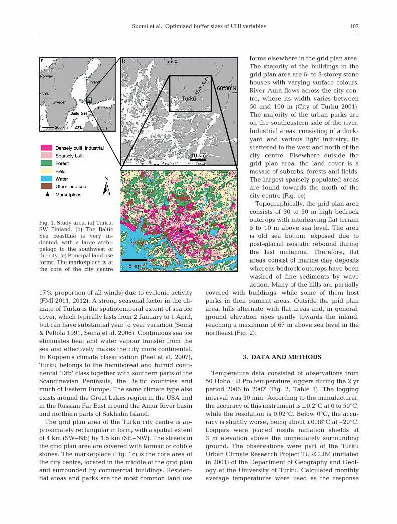
The study area consisted of the mid-sized (179 000inhabitants) coastal city Turku (city centre: 60° 27’ N,22° 16’ E) and parts of its neighbouring municipali-ties. The area is located in SW Finland at the mouthof the River Aura. The Baltic Sea coastline in theregion is very indented, exhibiting a large archipel-ago to the southwest of the city (Fig. 1a,b). Due to theeffects of nearby islands and the large archipelago,the climate of Turku is a mixture of coastal and inlandtypes. Depending on the location and movements oflarge weather systems, either continental or marinecharacteristics can dominate (Alalammi 1987). AtTurku airport, 7 km north of the city centre, theannual average temperature for the period 1981 to2010 was 5.5°C. February is typically the coldestmonth, while July is the warmest, with average tem-peratures of −5.2 and 17.5°C, respectively. The high-est temperature in the period 1981 to 2010 was32.1°C (2010) and the coldest was −34.8°C (1987).Mean annual precipitation is 723 mm, of which 30%falls as snow. The average duration of permanentsnow cover is approximately 90 d starting from 24December. The wettest month is typically August,while April is the driest, with monthly rainfalls of 80and 32 mm, respectively. Winds are highly variablein speed (average 3.4 m s−1; highest in November,December and January: 3.6 m s−1; and lowest inAugust: 3.1 m s−1) and direction (dominant SW with

106

Suomi et al.: Optimized buffer sizes of UHI variables

17% proportion of all winds) due to cyclonic activity(FMI 2011, 2012). A strong seasonal factor in the cli-mate of Turku is the spatiotemporal extent of sea icecover, which typically lasts from 2 January to 1 April,but can have substantial year to year variation (Seinä& Peltola 1991, Seinä et al. 2006). Continuous sea iceeliminates heat and water vapour transfer from thesea and effectively makes the city more continental.In Köppen’s climate classification (Peel et al. 2007),Turku belongs to the hemiboreal and humid conti-nental ‘Dfb’ class together with southern parts of theScandinavian Peninsula, the Baltic countries andmuch of Eastern Europe. The same climate type alsoexists around the Great Lakes region in the USA andin the Russian Far East around the Amur River basinand northern parts of Sakhalin Island.

The grid plan area of the Turku city centre is ap -proximately rectangular in form, with a spatial extentof 4 km (SW−NE) by 1.5 km (SE−NW). The streets inthe grid plan area are covered with tarmac or cobblestones. The marketplace (Fig. 1c) is the core area ofthe city centre, located in the middle of the grid planand surrounded by commercial buildings. Residen-tial areas and parks are the most common land use

forms elsewhere in the grid plan area.The majority of the buildings in thegrid plan area are 6- to 8-storey stonehouses with varying surface colours.River Aura flows across the city cen-tre, where its width varies between50 and 100 m (City of Turku 2001).The majority of the urban parks areon the southeastern side of the river.Industrial areas, consisting of a dock-yard and various light industry, liescattered to the west and north of thecity centre. Elsewhere outside thegrid plan area, the land cover is amosaic of suburbs, forests and fields.The largest sparsely populated areasare found towards the north of thecity centre (Fig. 1c)

Topographically, the grid plan areaconsists of 30 to 50 m high bedrockoutcrops with interleaving flat terrain5 to 10 m above sea level. The areais old sea bottom, exposed due topost-glacial isostatic rebound duringthe last millennia. Therefore, flatareas consist of marine clay depositswhereas bedrock outcrops have beenwashed of fine sediments by waveaction. Many of the hills are partially

covered with buildings, while some of them hostparks in their summit areas. Outside the grid planarea, hills alternate with flat areas and, in general,ground elevation rises gently towards the inland,reaching a maximum of 67 m above sea level in thenortheast (Fig. 2).

3. DATA AND METHODS

Temperature data consisted of observations from50 Hobo H8 Pro temperature loggers during the 2 yrperiod 2006 to 2007 (Fig. 2, Table 1). The logginginterval was 30 min. According to the manufacturer,the accuracy of this instrument is ±0.2°C at 0 to 50°C,while the resolution is 0.02°C. Below 0°C, the accu-racy is slightly worse, being about ±0.38°C at −20°C.Loggers were placed inside radiation shields at3 m elevation above the immediately surroundingground. The observations were part of the TurkuUrban Climate Research Project TURCLIM (initiatedin 2001) of the Department of Geography and Geol-ogy at the University of Turku. Calculated monthlyaverage temperatures were used as the response

107

Fig. 1. Study area. (a) Turku,SW Finland. (b) The BalticSea coastline is very in-dented, with a large archi-pelago to the southwest ofthe city. (c) Principal land useforms. The marketplace is atthe core of the city centre

Clim Res 55: 105–118, 2012

variables in the statistical analyses. A month wasconsidered the proper time span, as it is short enoughto reflect seasonal variation in independent effectsand explanatory powers of the variables. On theother hand, a month is long enough to smooth thevariation caused by short-term weather phenomena.

Altogether, 12 explanatory variables were includedin the first step of the analysis in which optimal buffersizes were determined (Tables 2 & 3). The land useand environmental variables included 6 urban and 6non-urban variables. The division into urban andnon-urban variables was made mainly based on ther-mal characteristics of the land use forms. The urbanvariables described densely built areas with a strongeffect on UHI. One of the urban variables, namely thebuilding floor area, was derived from the City ofTurku (2010) database. The other 5 urban variableswere obtained from the SLICES (2011) land use clas-sification. SLICES is a national mapping project initi-ated by the Ministry of Agriculture and Forestry andheaded and processed by the National Land Surveyof Finland. It consists of 45 land use classes, includingthe following main ones: A = residential and leisureareas; B = business, administrative and industrialareas; C = supporting activity areas; D = rock and soilextraction areas; E = agricultural land; F = forestryland; G = other land; and H = water areas.

Of the 6 non-urban variables, ‘industrial and ware-house areas’, ‘detached houses’ and ‘agriculturallands’ were derived from SLICES; ‘water bodies’

from SLICES and the CORINE landcover database (EEA 2006); ‘relativeele vation’ from a digital elevationmodel (DEM; NLS 2009); and ‘green-ness’ of tasseled cap transformationfrom Landsat ETM+ satellite images(cf. Crist & Cicone 1984, Hjort & Luoto2006). In tasseled cap transformation,the spectral bands’ pixel values areconverted to weighted sums of theoriginal values of a set of bands. Oneof these weighted sums, ‘greenness’,indicates the amount of green (i.e.photosynthetically active) vegetation,and it was selected as one variableinstead of the more commonly usednormalized difference vegetation in -dex (NDVI). The selection was basedon a preliminary analysis in which‘greenness’ showed a higher correla-tion with the temperature variables(using Spear man’s rank correlation rS

and optimal buffer sizes, the meanrS of monthly temperatures with ‘greenness’ and‘NDVI’ were −0.81 and −0.79, respectively). The spa-tial resolution of SLICES is 10 × 10 m, whereas theDEM and CORINE have a resolution of 25 × 25 m,and Landsat ETM+ imaging 30 × 30 m for bands usedin the computations. The values of the explanatoryvariables were computed using ArcGIS 9.3 and MSExcel 2003 software.

The theoretical maximum buffer sizes were deter-mined for each ex planatory variable based on the lit-erature and estimated thermal effects of the variable.In the literature, the radius of the buffers used or rec-ommended varied typically between 17 and 1500 m,whereas the UHI itself has been reported to extendup to 30 km in large towns (e.g. Hicks et al. 2010).Oke (1973) made comparisons between city size andmaximum UHI intensity. As UHI intensity strength-ens between 100 000 and 1 000 000 inhabitants, thecircle of influence is supposed to be >500 m, and insome cases even >1000 m. Stewart & Oke (2009)have also concluded that the circle of influence islarger in an open environment compared to that ofbuilt surroundings. Based on these facts, the theoret-ical maximum buffer size of most of the urban vari-ables was set at 2 km, and for most of the non-urbanvariables at 5 km (Table 3, Fig. 3). The theoreticalmaximum buffer size for ‘floor area’ was 300 mbecause the data were available only from Turku andKaarina municipalities, and larger buffers crossedtheir borders. For ‘water bodies’, a relatively large

108

Fig. 2. Topography of the study area. Numbers refer to temperature logger sites (see Table 1)

Suomi et al.: Optimized buffer sizes of UHI variables

maximum buffer size is justifiable, as the sea storesheat in a thick layer and releases latent heat withevaporation (see Hjort et al. 2011, Suomi & Käyhkö2012). Taking into account the characteristics of thestudy area and the extent of the observation network,the theoretical maximum buffer size for ‘water bod-ies’ was determined to be 20 km. A theoretical maxi-

mum buffer size for ‘relative elevation’ was set to1 km due to the present topographic features whosehorizontal extent is often <1 km (Table 3).

Spearman’s rank order correlation coefficientswere calculated between monthly average tempera-tures and explanatory variables to determine the op -timal buffer sizes. The correlation coefficients were

109

Logger no. Regional character Elevation Distance from city centre Land cover in the surroundings (m a.s.l.) (km)

1 Rural 2.4 9.8 Forest, gravel road2 Semi-urban 4.9 7.1 Forest, field3 Rural 0.4 6.2 Forest, reeds4 Rural 34.7 6.2 Forest, gravel road5 Semi-urban 9.3 6.0 Gravel field, 2-storey building6 Rural 15.1 6.2 Forest, gravel road7 Rural 1.5 5.2 Field, meadow8 Semi-urban 5.8 4.6 Parking lot, 2-storey building9 Rural 0.6 5.1 Field, forest10 Semi-urban 0.0 3.2 Gravel field, high grassland11 Semi-urban 21.2 2.9 Forest, block of flats12 Urban 4.6 2.8 Grassland, different-sized buildings13 Rural 24.9 3.7 Forest, agricultural buildings14 Urban 18.5 1.9 Block of flats, gravel field15 Semi-urban 5.8 2.9 Forest, asphalt road16 Semi-urban 19.9 1.3 Detached houses, park17 Urban 10.3 1.0 Park, asphalt road18 Urban 10.0 0.9 Railway, row houses19 Semi-urban 26.2 3.0 Parking lot, field20 Semi-urban 30.0 1.7 Park, 2-storey building21 Semi-urban 25.0 1.0 Forest, detached houses22 Urban 7.4 0.7 Asphalt road, block of flats23 Urban 27.4 0.4 Park, public buildings24 Urban (marketplace) 8.6 0.1 Asphalt road, block of flats25 Semi-urban 36.8 4.2 Block of flats, 2-storey building26 Urban 30.8 0.7 Block of flats, park27 Rural 41.2 2.6 Forest, landfill28 Semi-urban 20.0 1.2 Detached houses, gravel road29 Urban 9.6 0.9 Row houses, roads30 Semi-urban 19.9 1.8 Industrial, asphalt road31 Urban 22.9 1.0 Block of flats, asphalt road32 Urban 20.7 1.3 Park, asphalt road33 Semi-urban 15.0 3.8 Allotment garden houses, forest34 Urban park 20.0 1.6 Park, leisure-time areas35 Semi-urban 14.8 2.1 Detached houses, roads36 Semi-urban 20.1 3.6 Public buildings, detached houses37 Semi-urban 25.1 3.4 Forest, graveyard38 Semi-urban 30.0 2.6 Detached houses, roads39 Semi-urban 23.6 3.5 Detached houses, forest40 Rural 19.9 4.3 Field, roads41 Semi-urban 15.8 3.5 Forest, meadow42 Semi-urban 49.9 3.9 Block of flats, row houses43 Rural 20.0 5.2 Landfill, forest44 Rural 12.7 4.2 Field, forest45 Rural 34.6 9.9 Field, forest46 Semi-urban 45.2 5.1 Public buildings, block of flats47 Rural 21.5 7.5 Field, forest48 Semi-urban 56.4 11.1 Blocks of flats, asphalt road49 Rural 32.4 9.9 Forest, meadow50 Semi-urban 38.7 6.3 Detached houses, lake

Table 1. Temperature logger sites (see Fig. 2 for locations). Distance from city centre is measured from the centre point of themarketplace. Land cover includes the 2 most common land use forms inside a 100 m radius buffer based on the SLICES land

use classification

Clim Res 55: 105–118, 2012110

Step Data Method

1. Buffer size optimization 12 variables, see Table 3 Spearman’s rank correlation

2. Independent effects of urban variables 6 urban variables, see Table 3 Hierarchical partitioning

3a. Independent effects of 1 urban and ‘Best urban variable’ in Step 2, Hierarchical partitioning9 other variables 6 non-urban and 3 spatial variables

3b. Multivariate modelling Same as in Step 3a Linear regression

Table 2. Main steps of the analyses

Explanatory variables Potential buffer sizes (radius, m) Source of data

Urban Urban land use (Ul) 100, 200, 300, 500, 1000, 2000 SLICES (2011)Large and urban buildings (Lb) 100, 200, 300, 500, 1000, 2000 SLICES (2011)Floor area (Fl) 100, 200, 300 City of Turku (2010)Block of flats (Bf) 100, 200, 300, 500, 1000, 2000 SLICES (2011)Business and administrative areas (Ba) 100, 200, 300, 500, 1000, 2000 SLICES (2011)Traffic areas (Tr) 100, 200, 300, 500, 1000, 2000 SLICES (2011)

Non-urbanIndustrial and warehouse areas (In) 100, 200, 300, 500, 1000, 2000 SLICES (2011)Detached houses (Dh) 100, 200, 300, 500, 1000, 2000, 5000 SLICES (2011)Agricultural lands (Ag) 100, 200, 300, 500, 1000, 2000, 5000 SLICES (2011)Water bodies (Wa) 100, 500, 1000, 1500, 2000, 5000, 10000, 20000 SLICES (2011), CORINE (EEA 2006)Relative elevation (Re) 100, 200, 300, 500, 1000 DEM (NLS 2009)Tasseled cap greenness (Gr) 100, 200, 300, 500, 1000, 2000, 5000 Landsat ETM+ images (Crist &

Cicone 1984, Hjort & Luoto 2006)

Table 3. Potential buffer sizes (i.e. the circle of influence) of the explanatory variables. The largest potential buffer size of the variable is the theoretical maximum buffer size of that variable. DEM = digital elevation model

Fig. 3. Examples of theoretical maximum buffer sizes of the explanatory variables in relation to the study area. The centre of the buffers is the marketplace. Radius of the buffers: (a) 300, 1000, 2000 and 5000 m, (b) 20 000 m

Suomi et al.: Optimized buffer sizes of UHI variables 111

calculated for each of the potential buffer sizes(Table 3). For most of the variables, selection of theoptimal buffer size was based on the highest correla-tion coefficients. However, if a clear curve saturationor levelling off effect in the curve of the coefficientswas detected, the point of levelling off rather thanthe highest value was considered the optimum buffersize. The correlations were calculated with SPSS 19software.

After determining the optimal buffer size for eachex planatory variable, the relative independent effect(hereinafter referred to as ‘independent effect’) ofthe variables was investigated in HP (Steps 2 and 3ain Table 2). The HP method is designed to over-come multicollinearity problems (i.e. intercorrela -tion among explanatory variables) by using a mathe-matical hierarchical theorem by which the ex -planatory capacities of a set of explanatory variablescan be estimated (Chevan & Sutherland 1991, Mac-Nally 1996). HP employs goodness-of-fit measuresfor each of 2k possible models for k explanatory vari-ables. In HP, the variances are partitioned so that thetotal independent contribution of a given explana-tory variable can be estimated (Chevan & Sutherland1991). For example, the independent contribution ofthe ‘floor area’ variable is estimated by comparinggoodness-of-fit measures for all models including the‘floor area’ variable with their reduced version (i.e.the exact same model but without ‘floor area’) withineach hierarchical level; e.g. with 3 explanatory vari-ables (23), there are 8 possible models at 4 hierar -chical levels (models with only intercept, 1, 2 and 3variables). The average improvement in fit for eachhierarchical level that includes ‘floor area’ is thenaveraged across all hierarchies, giving the independ-ent contribution of the ‘floor area’ variable. Thus,HP allows one to differentiate between those ex -planatory variables whose independent, as distinctfrom partial, correlation with a response variablemay be important, from variables that have littleindependent effect on the studied phenomena. In thepresent study, HP was conducted using the ‘hier.part’package version 1.0-3 in statistical software R ver-sion 2.11.1 (http://r-project.org). The goodness-of-fitmeasure we used was root-mean-square predictionerror (RMSPE) (e.g. MacNally 2000). For every res -ponse variable, several regression models were gen-erated (64 in Step 2, and 1024 in Step 3a) to revealthe most meaningful explanatory variables in deter-mining monthly average temperatures.

In order to find the urban variable with thestrongest independent effect, the 6 intercorrelatedur ban variables were compared with each other in

HP (Step 2 in Table 2). Next, the selected urban vari-able of each month was taken into the further analy-sis, where the urban variable was modelled with 9other explanatory variables in HP (Step 3a in Table 2).In this step, spatial variables, namely eastern (X) andnorthern (Y) map coordinates (Finland UniformCoordinate System) and ‘distance from city centre’,were included in the HP in addition to the 6 land useand environmental variables. The spatial variableswere employed to cover the potential spatial struc-tures (i.e. trend and spatial autocorrelation) in theresponses not covered by any other explanatory vari-ables in the analyses. Consequently, the main focuswas on urban and non-urban variables, whereas thespatial variables served only as a control in this study.

As the second part of the final step, a multivariateLR (for LR, see Sokal & Rohlf 1995) was employed tomodel the observed temperature differences in thestudy area (Step 3b in Table 2). The calibration of theLR model was performed utilizing the standard lmfunction in R. The LR model optimization was basedon a step-wise approach and Akaike’s informationcriterion (AIC) (Akaike 1974, Burnham & Anderson1998). The normality of the distribution of variableswas tested before the HP and L R analyses. For caseswhose frequency-size distribution was not normal,different transformations were tested. If the variablecould not be transformed to meet the normalityassumption, the original variable was used (Sokal &Rohlf 1995). In general, LR has been used in severalUHI studies (e.g. Unger et al. 2001, Kim & Baik 2002,Unger 2006, Szymanowski & Kryza 2009, 2011,Yokobori & Ohta 2009), but to our knowledge, HP isa new method in the UHI context. HP has, however,been successfully utilized in the biosciences (e.g.MacNally 2000, Heikkinen et al. 2004) and geo -sciences (e.g. Hjort et al. 2007, Hjort & Luoto 2009).

4. RESULTS

4.1. Optimal buffer sizes

For urban variables, the radius of the optimal buffersizes varied be tween 300 and 1000 m, the largerone being the most common value (Table 4). Amongthe other variables, the optimal buffer size variedbetween 100 and 20 000 m, the mode being 2000 m.The average optimum buffer size of urban variableswas ca. 700 m, and for non-urban variables it was 2500m. Of all the variables, ‘water bodies’ had the largestaverage buffer size, 6100 m, and ‘relative elevation’the smallest one, 200 m.

Clim Res 55: 105–118, 2012

On a monthly basis, the average buffer size of all thevariables was largest in July and August (2700 m) andsmallest in April and May (1200 m). For the urbanvariables, the average buffer size was largest (900 m)from March to May, and smallest (500 m) from Sep-tember to February. For non-urban variables, the av-erage buffer size was largest (4600 m) in July and Au-gust, and smallest (1400 m) in April and May(Table 4). It should be noted that the average values ofthe optimal buffer sizes are used here only to illustratethe differences between variables and between vari-able groups, as well as seasonal differences of thevariable groups.

4.2. Independent effects of urban variables in HP

Based on HP, the ‘large and urban buildings’ vari-able had the highest independent explanatory power

of the 6 urban variables, the average proportionbeing 24.9% (Table 5). On average, the weakesturban variable, with an independent effect of 12.2%,was ‘urban land use’. Seasonally, ‘floor area’ hadthe largest independent effect in spring and earlysummer (from March to June), whereas in allother months, ‘large and urban buildings’ was the

112

Variable Jan Feb Mar Apr May Jun Jul Aug Sep Oct Nov Dec Avg.

Ul 300 300 1000 1000 1000 300 300 300 300 300 300 300 500 0.481** 0.544** 0.839** 0.836** 0.838** 0.831** 0.787** 0.764** 0.544** 0.421** 0.391** 0.489**

Lb 1000 1000 1000 1000 1000 1000 1000 1000 1000 1000 1000 1000 1000 0.548** 0.637** 0.860** 0.881** 0.879** 0.879** 0.849** 0.822** 0.589** 0.492** 0.454** 0.527**

Fl 300 300 300 300 300 300 300 300 300 300 300 300 300 0.478** 0.560** 0.876** 0.897** 0.903** 0.913** 0.852** 0.832** 0.570** 0.408** 0.368** 0.458**

Bf 1000 1000 1000 1000 1000 1000 1000 1000 1000 1000 1000 1000 1000 0.403** 0.509** 0.798** 0.800** 0.801** 0.789** 0.716** 0.696** 0.429** 0.329* 0.298* 0.387**

Ba 300 300 1000 1000 1000 1000 1000 1000 300 300 300 300 700 0.495** 0.558** 0.832** 0.844** 0.863** 0.861** 0.796** 0.767** 0.580** 0.466** 0.417** 0.498**

Tr 300 300 1000 1000 1000 1000 1000 1000 300 300 300 300 700 0.494** 0.542** 0.834** 0.889** 0.849** 0.852** 0.797** 0.760** 0.536** 0.426** 0.423** 0.517**

Avg. urban 500 500 900 900 900 800 800 800 500 500 500 500 700

In 2000 2000 2000 2000 2000 2000 2000 2000 2000 2000 2000 2000 2000 0.408** 0.481** 0.575** 0.585** 0.575** 0.562** 0.623** 0.612** 0.477** 0.402** 0.380** 0.391**

Dh 1000 1000 5000 5000 5000 5000 5000 5000 1000 1000 1000 1000 3000 −0.406** −0.333* 0.525** 0.571** 0.542** 0.546** 0.443** 0.420** −0.357* −0.443**−0.424** −0.374**

Ag 5000 5000 500 500 500 500 500 500 5000 5000 5000 5000 2800 −0.787** −0.815**−0.695**−0.614**−0.692**−0.707** −0.671**−0.709**−0.701**−0.758**−0.772** −0.729**

Wa 5000 5000 500 500 500 2000 20000 20000 5000 5000 5000 5000 6100 0.589** 0.578** −0.151 −0.131 −0.116 −0.110 0.146 0.233 0.510** 0.645** 0.664** 0.559**

Re 100 100 500 300 300 300 100 100 100 100 100 100 200 0.251 0.262 0.411** 0.311* 0.358* 0.342* 0.312* 0.349* 0.256 0.184 0.170 0.184

Gr 2000 2000 200 200 200 200 200 200 2000 2000 2000 2000 1100 −0.872** −0.879**−0.755**−0.758**−0.786**−0.818** −0.798**−0.788**−0.830**−0.832**−0.810** −0.807**

Avg. non-urban 2500 2500 1500 1400 1400 1700 4600 4600 2500 2500 2500 2500 2500

Avg. all 1500 1500 1200 1200 1200 1200 2700 2700 1500 1500 1500 1500 1600

Table 4. Determined optimal buffer sizes (m) and corresponding Spearman’s rank order correlation coefficients (italics) of the explanatoryvariables. Average (avg.) values (rounded to the nearest hundred) are calculated only for the buffer sizes. Significance: *p < 0.05, **p < 0.005.

See Table 3 for abbreviations

Urban variable Independent effect (%)

Ul 12.2 Lb 24.9 Fl 19.6 Bf 12.3 Ba 15.5 Tr 15.5

Table 5. Average independent effects of urban variablesbased on hierarchical partitioning analysis. See Table 3 for

abbreviations

Suomi et al.: Optimized buffer sizes of UHI variables

strongest variable (hereinafter the term ‘best urbanvariable’ is used for the strongest variable based onHP analysis). The highest and lowest single inde-pendent effects (32.1 and 9.5%, respectively) existedin November, the lowest being that of the ‘urban landuse’ variable (Fig. 4).

4.3. Independent effects of the best urban variableand non-urban variables in HP

The HP results indicated that the ‘best urban vari-able’ had on average the highest (21.2%) independ-ent effect on temperatures. The effect of ‘greenness’was almost as large (21.0%). The effect of ‘relativeelevation’ was on average the weakest (1.1%,Table 6). On a monthly basis, the ‘greenness’ vari-able had the highest independent explanatory powerin the 7 mo from August to February, whereas inother months, the ‘best urban variable’ was domi-nant. The highest single independent effect (30.7%)ex isted for ‘floor area’ in March and the lowest(0.3%) for ‘relative elevation’ in April (Fig. 5).

4.4. Linear regression

The results of LR modelling are presented inTable 7. According to the residual plots, the assump-tion of normal errors was appropriate. The adjustedR2 values of the models varied between 0.71 and0.91, being highest in March and lowest in Septem-ber. The ‘best urban variable’ was the most importantvariable during 5 months, whereas the ‘water bodies’variable dominated in 4 months. Seasonally, the ur -ban variables dominated mostly in spring, and ‘waterbodies’ in late autumn and early winter. ‘Greenness’was the most important variable in July and August,and ‘distance from city centre’ in May. The impact of‘best urban’ and ‘water body’ variables on tempera-ture was constantly positive, whereas the ‘greenness’and ‘distance from city centre’ variables had coolingeffects.

113

Fig. 4. Independent effects (% of total independently ex-plained variance) of the urban variables in explaining tem-perature variability by month, as estimated from hierarchical

partitioning. See Table 3 for abbreviations

Variable Independent effect (%)

Ur 21.2 In 5.4 Dh 5.8 Ag 12.1 Wa 5.1 Re 1.1 Gr 21.0 X 5.8 Y 5.5 Di 17.0

Table 6. Average independent effects of the ‘best urban vari-able’ (Ur) and non-urban variables. Distance from city centre(Di) is measured from the centrepoint of the marketplace. X =eastern map coordinate, Y = northern map coordinate.

See Table 3 for other abbreviations

Clim Res 55: 105–118, 2012114

5. DISCUSSION

The results of this study clearly indicate that whenpossible, it is important to explore the optimumbuffer sizes of explanatory variables before furtheranalyses of UHI. This is in contrast with the commonpractice in urban climate studies, where the em -ployed buffer sizes have often been based on the lit-erature or site-specific consideration. The results alsodemonstrate that the optimal buffer size of a certain

variable can have large seasonalvariation, which is important to takeinto account in UHI studies.

The determined optimal buffersizes of urban variables were either300 or 1000 m and thus settling underthe theoretical maximum buffer sizeset before the analyses. The observedbuffer sizes were consistent withOke’s (2006) estimation of 500 m forthe circle of influence, the size thathas been used by e.g. Eliasson &Svensson (2003) and Suomi & Käyhkö(2012). The determined buffer sizeswere, however, clearly larger thanthe 25 to 50 m estimated by Giridha-ran & Kolokotroni (2009). The differ-ence in optimum buffer sizes can,however, be partly due to differentexplanatory variables used in thestudies. The mode and average sizeof the non-urban variables’ optimalbuffers were larger than those of ur-ban variables. This observation is inline with Stewart & Oke’s (2009) andGiridharan & Kolokotroni’s (2009)conclusions that the circle of influ-ence is larger in open and sparselybuilt areas than in a densely built environment.

The optimal buffer sizes of urbanvariables were, on average, largestin spring, and smallest in autumnand winter. This finding is analogousto that of Giridharan & Kolokotroni(2009), who concluded that the opti-mal buffer size of on-site variableswas smaller in winter than in sum-mer. For non-urban variables, sea-sonal variation in optimal buffer sizesdiffered from the urban variables inthat the maximum sizes occurred inJuly and August and the smallest in

spring. This largely reflects the variation of the opti-mal buffer size of ‘water bodies’ between spring andsummer, i.e. 500 m in spring to 20 000 m in July andAugust (cf. Table 4). In variable-specific com par -isons, the optimal buffer size varied seasonally moreuniformly among urban variables than among non-urban variables; the optimal buffer size of ‘detachedhouses’ was largest (5000 m) from March to Septem-ber, whereas at the same time the optimal buffer sizeof ‘greenness’ and ‘agricultural lands’ was smallest

Fig. 5. Independent effects (% of total independently explained variance) ofthe ‘best urban variable’ (‘large and urban buildings’ or ‘floor area’) and 9other explanatory variables in explaining temperature variability by month, asestimated from hierarchical partitioning. Numbered ranks indicate the rela-tive importance of the variables in the final linear regression models (see

Table 7). See Tables 3 and 6 for abbreviations

Suomi et al.: Optimized buffer sizes of UHI variables

(200 and 500 m, respectively). Such a contrasting pat-tern was not ob served among the urban variables.The more heterogeneous optimal buffer sizevariation among the non-urban variables is probablydue to the more versatile spectrum of factors thatthey reflect. In addition, for the urban variables, thecorrelation between them and temperatures is inevery case positive, whereas for the non-urban vari-ables, the direction of the correlation varies both be-tween and within variables.

Based on HP results for the urban variables, ‘largeand urban buildings’ and ‘floor area’ showed thehighest independent effect on temperatures, ca.20 to 30% depending on the month. ‘Floor area’dominated in spring and early summer, whereas‘large and urban buildings’ dominated in other sea-sons. As the latter variable is a combination ofblocks of flats, administrative and business areasand industrial and warehouse areas, it mostly re -flects the warming impact of buildings, similar tothe ‘floor area’ variable. Logically, the variablesconsisting of buildings and the variable consistingmainly of asphalt surfaces, namely ‘traffic areas’,showed the greatest difference in winter and lateautumn, when the solar heat storage of streets isminimal. Somewhat surprising, however, was thefinding that ‘traffic areas’ contributed in UHI only alittle also in summer. This can be partly due to thefact that ‘traffic areas’ included also relatively opensuburban and rural areas, where released radiation

was not trapped in nearby buildings, aswas the case in the city centre. Thelarger impact of building-based vari-ables compared to traffic areas was alsodetected by Hart & Sailor (2009) in day-time UHI modelling in June in Portland,Oregon. They found clear differencesbe tween weekdays and week ends, withthe average heat island intensity nearthe main arterial roads being 1.9°C onweekdays and 0.6°C on weekends. Thisindicates a relatively large effect of traf-fic compared to solar heat storage inroad areas. In Turku, the anthropogeniccomponent of the warming effect oftraffic areas is relatively low on smallersuburban and rural roads, which is onereason for the weak contribution of the‘traffic areas’ variable on UHI. In addi-tion, traffic has a relatively minor impactat night, and the heat flux from horizon-tal surfaces decreases towards the endof the night (see e.g. Kuttler et al. 1996),

which also diminishes the warming effect of trafficareas on average temperatures.

In a comparison between the ‘best urban variable’and the non-urban variables, the urban variable hadon average the highest independent impact based onHP. In LR, the ‘best urban variable’ was most oftenthe strongest, (in 5 out of 12 months) and it wasincluded in the model every month. Based on bothmethods, the dominance of the ‘best urban variable’was most ob vious in spring and early summer. Thismay be due to relatively cold sea areas during spring,which highlights the heating effect of the urban vari-ables. In Gothenburg, the variables reflecting urbaneffects were also strongest compared to other vari-ables in spring nights (Eliasson & Svensson 2003).

Among the non-urban variables, ‘greenness’ and‘water bodies’ dominated, although with some differ-ences, depending on the employed method; ‘green-ness’ dominated in HP and ‘water bodies’ in LR. Oneshould not directly compare the results of LR to HP,or consider either of these more correct, as these arerather different modelling approaches. HP is used toreveal independently the most important variablesamong correlated explanatory variables, whereasthe output of LR is a multivariate model (Chevan &Sutherland 1991, Sokal & Rohlf 1995). In the presentstudy, the explanatory power of ‘greenness’ waspartly or mostly covered by other variable(s) in thefinal LR models (cf. MacNally 2000). Compared withthe other rural variable, namely ‘agricultural lands’,

115

Adjusted R2 Ur In Dh Ag Wa Re Gr X Y Di

Jan 0.82 2,+ 1,+ 3,− 4,−

Feb 0.85 1,+ 3,+ 4,− 5,− 2,−

Mar 0.91 1,+ 3,+ 7,− 6,− 2,+ 5,− 4,−

Apr 0.88 1,+ 3,+ 2,−

May 0.87 2,+ 5,− 4,− 3,− 1,−

Jun 0.86 1,+ 4,− 3,− 2,−

Jul 0.84 4,+ 2,+ 1,− 6,+ 3,+ 5,−

Aug 0.86 2,+ 3,+ 1,− 4,+

Sep 0.71 1,+ 3,+ 2,−

Oct 0.80 2,+ 1,+ 3,− 4,−

Nov 0.82 3,+ 1,+ 4,− 2,−

Dec 0.74 2,+ 1,+ 3,−

Table 7. Linear regression (LR). The relative importance (rank) of the ex-planatory variable is also indicated (variables in the final LR models wereranked based on Akaike’s information criterion). + and −: direction of theeffect of the explanatory variables. See Tables 3 & 6 for abbreviations

Clim Res 55: 105–118, 2012

‘greenness’ clearly had stronger explanatory power.This may be due to the fact that forests were notincluded in the ‘agricultural lands’ variable, but theireffect was seen in ‘greenness’ values; in forested andvegetated areas, evapotranspiration is relativelyhigh, resulting in lower temperatures. Also, ‘green-ness’ was the most important variable in LR in mid-and late summer (July and August), when the abun-dance of vegetation is highest.

In addition to the strong effect of ‘greenness’ insummer, when using HP, its importance was also re-vealed in autumn and winter, when the verdancy ofvegetation is low. This finding is believed to originateat least partially in the low amount of anthropogenicheat sources in green areas (Crist & Cicone 1984).Moreover, ‘greenness’ as a continuous variable wasable to better reflect the lack of heat sources than thecategorical variables (e.g. agricultural areas). NDVIhas been commonly used in UHI studies (see e.g.Chen et al. 2006, Zhang et al. 2009, Szymanowski &Kryza 2011), but in our analyses, ‘greenness’ outper-formed NDVI in the preliminary correlation analysis.Consequently, the use of a greenness index is worthconsidering in urban climate studies.

Methodologically, traditional regression tech-niques may distort inferences about the relative im -portance of explanatory variables (Chevan & Suther-land 1991) because they lack sensitivity to detectintercorrelation be tween the explanatory variables(Sokal & Rohlf 1995). The HP method used in thepresent study provided a successful separate meas-ure of the amount of variation explained independ-ently by 2 or more ex planatory variables and, there-fore, it helped to make deductions on the importantenvironmental determinants (MacNally 1996, 2000).However, one should be aware of a couple of con-straints when using this ap proach. Firstly, HP doesnot produce a model and, secondly, the importanceof polynomial variables (i.e. non linear relationshipsbetween response and ex plana tory variables) cannotbe assessed. Consequently, HP is a suitable methodfor exploring causal variables, but it is not suited fore.g. predicting temperatures. However, the relation-ships between temperature and environmental vari-ables in UHI studies have often been reported to belinear, and thus the difficulty of investigating non -linear responses is potentially a minor short coming inthe UHI context (e.g. Eliasson & Svensson 2003).Finally, rather than considering LR and HP as exclu-sionary methods, it is advisable to combine them inmultivariate analyses, especially if explanatory vari-ables are highly intercorrelated (MacNally 2000,Heikkinen et al. 2004, Hjort & Luoto 2009).

6. CONCLUSIONS

Based on our results, we can draw 4 main conclu-sions. (1) The comparison of the 6 urban and 6 non-urban explanatory variables on different scalesrevealed that the optimal buffer size radius of theurban variables varied seasonally, being either 300 or1000 m. For the non-urban variables, the optimalmonthly buffer size showed larger variation; be -tween 100 and 20 000 m, the mode being 2000 m.

(2) The optimal buffer size of the urban variableswas largest in spring and smallest in winter andautumn. For the non-urban variables, no clear sea-sonal trend was observed.

(3) Of the 6 intercorrelated urban variables, ‘largeand urban buildings’ and ‘floor area’ had the largestindependent impact on temperatures. This indicatesthat in our high-latitude study area, heat releasedfrom buildings dominates in UHI formation through-out the year over heat released from horizontal urbansurfaces.

(4) In the comparison between the ‘best urban vari-able’ and 6 non-urban variables, HP revealed thehigh importance of the ‘urban’ and Landsat ETM+based ‘greenness’ variables, whereas LR highlightedthe importance of the ‘urban’ and ‘water body’ variables.

Acknowledgements. The Finnish Cultural Foundation’sVarsinais-Suomi Regional Fund, Emil Aaltonen Foundationand Turku University Foundation provided financial supportin the form of personal scholarships (J.S.). The TURCLIMproject collaborates with the Turku Environment and CityPlanning Department, whose assistance is of great value.The long-term reference weather data were provided by theFinnish Meteorological Institute.

LITERATURE CITED

Akaike H (1974) A new look at statistical model identifica-tion. IEEE Trans Automat Control 19: 716−723

Alalammi P (1987) Atlas of Finland: 131, Climate. NationalBoard of Survey, Geographical Society of Finland,Helsinki

Burnham KP, Anderson DR (1998) Model selection andinference: a practical information-theoretic approach.Springer, New York, NY

Chen XL, Zhao HM, Li PX, Yin ZY (2006) Remote sensingimage-based analysis of the relationship between urbanheat island and land use/cover changes. Remote SensEnviron 104: 133−146

Chevan A, Sutherland M (1991) Hierarchical partitioning.Am Stat 45: 90−96

City of Turku (2001) General plan 2020. Environmental andCity Planning Department, Plan Office, Turku

City of Turku (2010) Floor area of the buildings. Real EstateDepartment, Turku

116

Suomi et al.: Optimized buffer sizes of UHI variables

Costa A, Labaki L, Araujo V (2007) A methodology to studythe urban distribution of air temperature in fixed points.In: Santamouris M, Wouters P (eds) 2nd PALENC and28th AIVC Conference: Building Low Energy Coolingand Advanced Ventilation Techno logies in the 21st Cen-tury, 27–29 Sep 2007, Crete, p 227–230

Cotton WR, Pielke RA (1995) Human impacts on weatherand climate. Cambridge University Press, Cambridge

Crist EP, Cicone RC (1984) Application of the tasseled capconcept to simulated Thematic Mapper data. Photo -gramm Eng Remote Sens 50: 343−352

EEA (European Environment Agency) (2006) CORINE landcover. EEA, Denmark

Eliasson I, Svensson MK (2003) Spatial air temperature vari-ations and urban land use — a statistical approach. Mete-orol Appl 10: 135−149

FMI (Finnish Meteorological Institute) (2011) Ilmasto-opas.http: //ilmasto-opas.fi/fi/

FMI (Finnish Meteorological Institute) (2012) TilastojaSuomen ilmastosta 1981–2020. www.ilmatieteenlaitos.fi

Giridharan R, Kolokotroni M (2009) Urban heat island char-acteristics in London during winter. Sol Energy 83: 1668−1682

Giridharan R, Lau SSY, Ganesan S, Givoni B (2007) Urbandesign factors influencing heat island intensity in high-rise high-density environments of Hong Kong. BuildEnviron 42: 3669−3684

Giridharan R, Lau SSY, Ganesan S, Givoni B (2008) Lower-ing the outdoor temperature in high-rise high-densityresidential developments of coastal Hong Kong: vegeta-tion influence. Build Environ 43: 1583−1595

Hart MA, Sailor DJ (2009) Quantifying the influence of lan-duse and surface characteristics on spatial variability inthe urban heat island. Theor Appl Climatol 95: 397−406

Heikkinen RK, Luoto M, Virkkala R, Rainio K (2004) Effectsof habitat cover, landscape structure and spatial vari-ables on the abundance of birds in an agricultural–forestmosaic. J Appl Ecol 41: 824−835

Hicks BB, Callahan WJ, Hoekzema MA (2010) On the heatislands of Washington, DC, and New York City, NY.Boundary-Layer Meteorol 135: 291−300

Hjort J, Luoto M (2006) Modelling patterned ground distri-bution in Finnish Lapland: an integration of topographi-cal, ground and remote sensing information. Geogr AnnA 88: 19−29

Hjort J, Luoto M (2009) Interaction of geomorphic and eco-logic features across altitudinal zones in a subarctic land-scape. Geomorphology 112: 324−333

Hjort J, Luoto M, Seppälä M (2007) Landscape scale deter-minants of periglacial features in subarctic Finland: agrid-based modelling approach. Permafrost PeriglacProcess 18: 115−127

Hjort J, Suomi J, Käyhkö J (2011) Spatial prediction ofurban-rural temperatures using statistical methods.Theor Appl Climatol 106: 139−152

Houet T, Pigeon G (2011) Mapping urban climate zones andquantifying climate behavior — an application onToulouse urban area (France). Environ Pollut 159: 2180−2192

Kim Y, Baik J (2002) Maximum urban heat island intensity inSeoul. J Appl Meteorol 41: 651−659

Kolokotroni M, Giridharan R (2008) Urban heat island inten-sity in London: an investigation of the impact of physicalcharacteristics on changes in outdoor air temperature

during summer. Sol Energy 82: 986−998Kuttler W, Barlag AB, Rossmann F (1996) Study of the

thermal structure of a town in a narrow valley. AtmosEnviron 30: 365−378

Landsberg HE (1981) The urban climate. Academic Press,London

MacNally R (1996) Hierarchical partitioning as an interpre-tative tool in multivariate inference. Aust J Ecol 21: 224−228

MacNally R (2000) Regression and model-building in con-servation biology, biogeography and ecology: the dis-tinction between — and reconciliation of — ‘predictive’and ‘explanatory’ models. Biodivers Conserv 9: 655−671

NLS (National Land Survey of Finland) (2009) Digital eleva-tion model. NLS, Helsinki

Oke TR (1973) City size and the urban heat island. AtmosEnviron 7: 769−779

Oke TR (1987) Boundary layer climates, 2nd edn. Routledge,London

Oke TR (2006) Initial guidance to obtain representativemeteorological observations at urban sites. Instrumentsand Observing Methods Report No. 81. World Meteoro-logical Organization, Geneva

Peel MC, Finlayson BM, McMahon TA (2007) Updatedworld map of the Köppen-Geiger climate classification.Hydrol Earth Syst Sci 11: 1633−1644

Sakakibara Y, Matsui E (2005) Relation between heat islandintensity and city size indices/urban canopy characteris-tics in settlements of Nagano basin, Japan. Geogr RevJpn 78: 812−824

Seinä A, Peltola J (1991) Duration of the ice season and sta-tistics of fast ice thickness along the Finnish coast 1961–1990. Finn Mar Res 258: 1–46

Seinä A, Eriksson P, Kalliosaari S, Vainio J (2006) Ice sea-sons 2001-2005 in Finnish sea areas. Report Series No.57. Finnish Institute of Marine Research, Helsinki

SLICES (2011) SLICES Maankäyttö. National Land Sur-vey of Finland. www.maanmittauslaitos. fi/ digituotteet/slices-maankaytto

Sokal RR, Rohlf FJ (1995) Biometry. WH Freeman, NewYork, NY

Stewart ID, Oke TR (2009) Classifying urban climate field sitesby ‘local climate zones’: the case of Nagano, Japan. In: Pre -prints, 7th Int Conf Urban Climate, 29 Jun−3 Jul, Yokoha -ma. www.ide.titech.ac.jp/~icuc7/extended_ abstracts/ pdf/385055-1-090515165722-002.pdf

Suomi J, Käyhkö J (2012) The impact of environmental fac-tors on urban temperature variability in the coastal city ofTurku, SW Finland. Int J Climatol 32: 451−463

Szymanowski M, Kryza M (2009) GIS-based techniques forurban heat island spatialization. Clim Res 38: 171−187

Szymanowski M, Kryza M (2011) Application of geographi-cally weighted regression for modelling the spatial struc-ture of urban heat island in the city of Wroclaw (SWPoland). Proc Environ Sci 3: 87−92

Unger J (2006) Modelling of the annual mean maximumurban heat island using 2D and 3D surface parameters.Clim Res 30: 215−226

Unger J, Sümeghy Z, Gulyás Á, Bottanyán Z, Mucsi L (2001)Land-use and meteorological aspects of the urban heatisland. Meteorol Appl 8: 189−194

Wen X, Yang X, Hu G (2011) Relationship between landcover ratio and urban heat island from remote sensingand automatic weather stations data. J Indian Soc

117

Clim Res 55: 105–118, 2012

Remote Sens 39: 193−201Wong NH, Jusuf SK, Syafii NI, Chen Y, Hajadi N, Sathya-

narayanan H, Manickawasagam YV (2011) Evaluation ofthe impact of the surrounding urban morphology onbuilding energy consumption. Sol Energy 85: 57−71

Yokobori T, Ohta S (2009) Effect of land cover on air temper-

atures involved in the development of an intra-urbanheat island. Clim Res 39: 61−73

Zhang Y, Odeh IOA, Han C (2009) Bi-temporal characteriza-tion of land surface temperature in relation to impervioussurface area, NDVI and NDBI, using a sub-pixel imageanalysis. Int J Appl Earth Obs Geoinf 11: 256−264

118

Editorial responsibility: Helmut Mayer, Freiburg, Germany

Submitted: May 10, 2012; Accepted: July 10, 2012Proofs received from author(s): November 12, 2012