effects of illumination shadows in interference pattern

Effects of Illumination Shadows in Interference Pattern Structured Illumination Imaging

Carter Flanary Day

A senior thesis submitted to the faculty ofBrigham Young University

in partial fulfillment of the requirements for the degree of

Bachelor of Science

Dallin S. Durfee and Richard L. Sandberg, Advisor

Department of Physics and Astronomy

Brigham Young University

Copyright © 2020 Carter Flanary Day

All Rights Reserved

ABSTRACT

Effects of Illumination Shadows in Interference Pattern Structured Illumination Imaging

Carter Flanary DayDepartment of Physics and Astronomy, BYU

Bachelor of Science

Here I present a study on the effect of "large" three-dimensional objects in Interference PatternStructured Illumination Imaging (IPSII). Due to the nature of the IPSII method, objects with alot of depth in the imaging field create "shadows" or areas where the structured illumination failsThis is because IPSII’s structured illumination may be projected at a given angle θ from the objectnormal. These shadows are characterized by the absence of interference, not always the absence oflight, and cause blurring around edges in the resulting image. The more depth an object has, themore fringe effects appear in the resulting image. This thesis reviews simulations that capture thisreduced interference and therefore breakdown of IPSII due to shadowing. Also, initial experimentalresults are presented in an effort to demonstrate this effect. Finally, a discussion of what next stepsshould be taken is presented.

Keywords: senior thesis, undergraduate research, IPSII, imaging, optics

ACKNOWLEDGMENTS

I would like to thank Drs. Dallin Durfee, Richard Sandberg, and Jarom Jackson for their

incalculable guidance and mentorship throughout this project. This thesis would not be possible

without them. I would like to also thank my wife, Chelsea, for her patience, understanding, and help

with my writing during this time. I’ve spent many hours worrying about this paper, and through it

all she has been there with me.

Contents

Table of Contents v

1 Introduction 11.1 IPSII . . . . . . . . . . . . . . . . . . . . . . . . . . . . . . . . . . . . . . . . . . 21.2 MAS-IPSII . . . . . . . . . . . . . . . . . . . . . . . . . . . . . . . . . . . . . . 31.3 Shadows . . . . . . . . . . . . . . . . . . . . . . . . . . . . . . . . . . . . . . . . 6

2 Simulating the Characteristic Effects 72.1 One dimension . . . . . . . . . . . . . . . . . . . . . . . . . . . . . . . . . . . . 72.2 Two dimensions . . . . . . . . . . . . . . . . . . . . . . . . . . . . . . . . . . . . 8

2.2.1 Asymmetric results . . . . . . . . . . . . . . . . . . . . . . . . . . . . . . 9

3 Experimental IPSII Shadows 133.1 Recreating IPSII . . . . . . . . . . . . . . . . . . . . . . . . . . . . . . . . . . . . 13

3.1.1 Setup . . . . . . . . . . . . . . . . . . . . . . . . . . . . . . . . . . . . . 153.1.2 Image Results . . . . . . . . . . . . . . . . . . . . . . . . . . . . . . . . . 16

4 Conclusion 21

Appendix A 23A.1 1D IPSII Simulation Code . . . . . . . . . . . . . . . . . . . . . . . . . . . . . . 23A.2 2D IPSII Shadow Mask Code (POV-Ray) . . . . . . . . . . . . . . . . . . . . . . 24A.3 2D IPSII Simulation Code . . . . . . . . . . . . . . . . . . . . . . . . . . . . . . 25

Appendix B 27

List of Figures 29

Bibliography 31

v

Chapter 1

Introduction

Throughout recent years, a wide array of imaging methods have been developed and better con-

structed for scientific research. Magnetic Resonance Imaging (MRI) in medicine provides clear

images of inside the body, allowing doctors and healthcare professionals to give better patient

care. Microscopy uses well-placed optical lenses to allow biologists to see and classify organisms

invisible to the naked eye, organisms like the SARS-CoV-2 virus which causes the COVID-19

disease. Interference Pattern Structured Illumination Imaging (IPSII) supplies scientists with a

non-invasive way to image objects on a relatively small scale. IPSII is a lensless, single-pixel

imaging method meant to circumvent conventional imaging limitations. Currently, it is still in its

early stages of development.

Previous iterations of IPSII like DEEP tomography [1], CHIRPT [2], and SWIF [3] have proved

the concept successful in imaging. In recent years, a Mechanical Angle Scan (MAS) implementation

of IPSII was developed by Jarom Jackson and Dallin Durfee at Brigham Young University [4–7].

Conventional imaging methods like the use of a microscope require high numerical aperture

objective lenses to acquire high resolution. That means a large objective lens with a short focal

length and a small distance between the objective lens and the object plane. IPSII works around

the short working distance by using structured illumination projected onto the object, allowing our

1

2 Chapter 1 Introduction

working distance to be as far as we can project the structured illumination pattern. We emphasize

here that this restricts the sample volume imaged with MAS-IPSII to the region where the two

illuminating beams overlap. In traditional lens-based microscopy, the depth of field (DOF) is the

volume where the sample will all remain in focus. Regions outside of the DOF (typically regions

axially, or along the beam propagation direction, outside the plane of best focus) will become

blurred. The DOF is directly related to the numerical aperture and has an inverse relation to the

resolution of the image. Because IPSII only uses flat optics and not an objective lens, the numerical

aperture is as wide as we make it to be, allowing us not to be as limited by the DOF.

IPSII has a theoretical maximum resolution of a quarter of the wavelength of light used [4].

Due to the nature of the method however, objects with a lot of axial extent or depth in the imaging

field create “shadows” or areas where the structured illumination fails due to one of the structured

illuminating beam being blocked by the object. These areas are not necessarily characterized by

the absence of light, but rather by the absence of interference, and cause blurring around edges

in the resulting image. What follows is an analysis of these effects. In particular, I will discuss

how three-dimensional objects cause aberrations in the resulting image due to the method itself and

the objects’ size or depth in the imaging field. I will begin by talking more about IPSII and how it

works, followed by a more in-depth study of MAS-IPSII and what "shadows" are in this context. In

Chapter 2 I will focus on computational simulations of these shadow effects, and in Chapter 3 I will

focus on the experimental verification of these shadow effects in MAS-IPSII.

1.1 IPSII

Interference Pattern Structured Illumination Imaging (IPSII) uses structured illumination and a

single pixel detector to record the reciprocal or Fourier space (here denoted as k-space) data of an

object being imaged, one k-space pixel at a time. Each data point consists of the light reflected off

1.2 MAS-IPSII 3

or transmitted through the object using a unique pattern. The resulting array of pixels is then run

through a mathematical transform to make a digital image of the object. Previous versions of this

method like DEEP tomography [1] have used acousto-optic modulators to change the structured

illumination for each data point.

The basic concept of IPSII uses an arbitrary illumination pattern projected onto an object and a

recording of the light reflected or transmitted. Based on the pattern chosen, the detected light is

then used to work backward to find what the object looks like. When using sinusoidal illumination

patterns, the array of data can be analyzed with the well-known Fourier transform and the method

becomes simpler in theory.

1.2 MAS-IPSII

Mechanical Angle Scan (MAS)-IPSII uses a Mach-Zehnder interferometer with motorized mirror

adjustments to alter the structured illumination for each data point, and scans the phase using a

piezo stack mounted behind a mirror in one of the beam paths as seen in Fig. 1.1. Currently the

most advanced design uses an extra set of mirrors in the interferometer to keep the illumination

pattern trained on the object and reference pinhole when the mirrors are adjusted to change the

pattern. This allows for larger angles between beams. Also, it contains a double bow tie design

immediately after the first beamsplitter as shown in Fig. 1.1b to help with balancing.

When two coherent plane waves interfere, a sinusoidal pattern of light and dark fringes are

created as in Fig. 1.2. The size of the fringes and the spacing between them is determined by the

angle between the incoming waves (i.e. the larger the angle, the smaller the fringe). The smallest

fringe size possible is a quarter of the wavelength of light used. In structured illumination (SI)

imaging, the resolution is limited to the scale of features that can be created in the illumination.

Therefore, using interference fringes, SI should theoretically be able to reach resolutions as small as


(a) (b)

Figure 1.1 (a) Working IPSII setup with minimal amount of optics. (b) A more complexoptical design for an interferometer with better beam control and path-length tuning.

(a) (b)

Figure 1.2 Two plane wave beams cross. Where they overlap, the plane waves interferewith each other to produce an sinusoidal pattern of fringes. The size and spacing of thefringes changes as the angle between the beams increases.

a quarter of the wavelength of light. This theoretical limit is one of the reasons MAS-IPSII was

designed.

Using the mirror movements to alter the structured illumination makes the necessary transform

easy because the projected pattern is approximated to a sinusoidal wave as it is scanned across the

object and reference pinhole as in Fig. 1.3 and therefore can be analyzed by means of a Fourier

transform.

1.2 MAS-IPSII 5

Figure 1.3 Two beams overlap to form a sinusoidal interference pattern on an object.

Figure 1.4 Two plane wave beams intersect and interfere. The size and spacing of thefringes changes as the angle between the beams increases. The Depth of Field (DOF) isthe area where they interfere (i.e. inside the green diamond).

A difficulty that arises due to the use of an interferometer is the limited depth-of-field (DOF), the

region in front of and behind the object plane in which the laser beams interfere. DOF is determined

by the diameter of the beams and the angle between them, and is generally characterized by the

maintenance of structured illumination (see Fig. 1.4). Clear imaging occurs only when the object is

in the DOF, leading to a limitation on the object depth as well as object placement. Object depth

refers to objects with axial extent in the direction of the illumination projection.


Figure 1.5 Two beams overlap to form a sinusoidal interference pattern on a cylinder asseen from the side. Immediately to the sides of the cylinder, light from only one beamreaches the surface and there is a lack of interference.

1.3 Shadows

"Shadows" in IPSII are regions in the imaging plane where the structured illumination fails. This

occurs by complete or partial blockage of the light generally due to axial extent (depth) in the DOF.

When an object with significant depth is imaged, these shadows can cause noticeable blurring in the

resulting image. As an example, imagine trying to image a cylinder like in Fig. 1.5. As the beam

coming from below arrives at the object, it is blocked from reaching the background plane at the

base of the cylinder on the top side. The same applies for the beam coming from above, but it is

blocked near the base below the cylinder. The structured illumination therefore has failed in those

regions near the base of the cylinder opposite to the incoming beams. These areas are what we refer

to as IPSII shadows.

Chapter 2

Simulating the Characteristic Effects

In this chapter, I will describe the process I took for developing one- and two-dimensional models

for simulating IPSII in Python. I will also present and discuss my IPSII reconstruction image results

for three separate situations.

2.1 One dimension

In the beginning of my research I developed a one-dimensional model for proof-of-concept of

IPSII shadows, owing to the idea that the shadows would cause simple aberrations in the image

surrounding the object.

All things have reflectivity, defining how much light they reflect when it is bounced off their

surface. The reflectivity (R) of an object is represented as a number between 0 and 1, 0 being

completely absorptive and 1 being completely reflective. The 1D model of MAS-IPSII in reflection

geometry that I developed in Python (see Appendix A.1) has three steps to simulate the IPSII

process. First, I set the angle of the beams and determine where the shadows are formed. Second, I

perform a Fourier transform (2.1) on the reflectivity with the shadow mask (S) multiplied inside

the integral. Third, I perform an inverse Fourier transform (2.2) on the answer to Eq. (2.1). I use a

7

8 Chapter 2 Simulating the Characteristic Effects

discrete sum to transform the reflectivity of the object:

F =N

∑n=0

S(Re−i 2πxnN ), (2.1)

Rnew =1

2π

N

∑n=0

F ei 2πxnN , (2.2)

where R is the reflectivity, S is the shadow mask, N is the size of the function, and Rnew is the

reflected light we would actually see, or rather, it is the resulting image reconstruction of the

reflectivity of the object.

The next section contains a description of the two-dimesnional model I made, and also contains

IPSII image reconstructions that demonstrate the effects of IPSII shadows.

2.2 Two dimensions

Treating the structured illumination as a sinusoidal pattern from an interferometer output, we can

model the IPSII process in reflection geometry using a 2D Fourier transform. The shadows then are

represented by a 2D mask (S) in the forward transform (2.3).

F =Nrow

∑m=0

Ncol

∑n=0

S(Re−i2πmxmy

NcolNrow ), (2.3)

Rnew =1

2π

Nrow

∑m=0

Ncol

∑n=0

F ei2πmxmy

NcolNrow , (2.4)

where Ncol is the number of columns (or the "length" in the x-direction), Nrow is the number of rows,

and Rnew is the resulting image of the reflectivity of the object.

2.2 Two dimensions 9

(a) (b)

Figure 2.1 POV-Ray cylinder and mask. (a) Blue cylinder as viewed from above. It isilluminated by two light sources placed at very far distances above the viewpoint andopposite to each other. (b) The mask of zeros and ones representing where the shadow isformed.

2.2.1 Asymmetric results

In deriving a two-dimensional model, I needed a way to create a different shadow mask for each

k-space value. I used Persistence of Vision Raytracer [8] to create an image of a simple cylinder as

viewed from above with two infinitely far light sources coming at opposite and equal angles from

each other onto it as in Fig. 2.1a (see Appendix A.2 for code). The light sources approximate to

laser beams in the context of the experiment. Each image with different angles for the light sources

was then stripped of everything but the shadows and set to zeros and ones as in Fig. 2.1b. The result

was a unique shadow mask I could apply to each k-space value during the 2D Fourier transform.

I applied the masks created through POV-ray to the cylinder object with three distinct reflectivi-

ties for the object top and background. In Figure 2.3, the top of the object is completely absorbent

(zero reflectivity) and the background is completely reflective (reflectivity of one). In that test, the

resulting image of the object shows aberrations around the object and the object is definitely visible


Figure 2.2 A height map of the cylinder object to simulate IPSII made in Python.

(a) (b) (c)

Figure 2.3 Simulation of IPSII reconstruction of cylinder object (Fig. 2.2) with differentnumber of k-space measurements: (a) 128×128 pixels, (b) 256×256 pixels, (c) 512×512pixels. Object face is completely absorptive (R = 0) and background is completely reflec-tive (R = 1).

as is expected. In Figure 2.4, both the top of the object and the background are completely reflective

(reflectivity of one). Since we are taking an image of the reflectivity and in this case the reflectivity

is the same everywhere, we could expect to see a blank image (uniform). However, the resulting

image shows aberrations around the object again, and the object is definitely visible contrary to

what we expected. In the last case (Fig. 2.5), the reflectivity of the object top and background were

both randomized (each point was given a random reflectivity between zero and one). This could

represent a bumpy surface where light hitting the surface would bounce off in any direction and only

2.2 Two dimensions 11

(a) (b) (c)

Figure 2.4 Simulation of IPSII reconstruction of cylinder object (Fig. 2.2) with differentnumber of k-space measurements: (a) 128×128 pixels, (b) 256×256 pixels, (c) 512×512pixels. Object face is completely reflective (R = 1) and background is completely reflective(R = 1).

(a) (b) (c)

Figure 2.5 Simulation of IPSII reconstruction of cylinder object (Fig. 2.2) with differentnumber of k-space measurements: (a) 128×128 pixels, (b) 256×256 pixels, (c) 512×512pixels. Object face and background have completely randomized reflectivities (R =random number, 0 ≤ R ≤ 1).


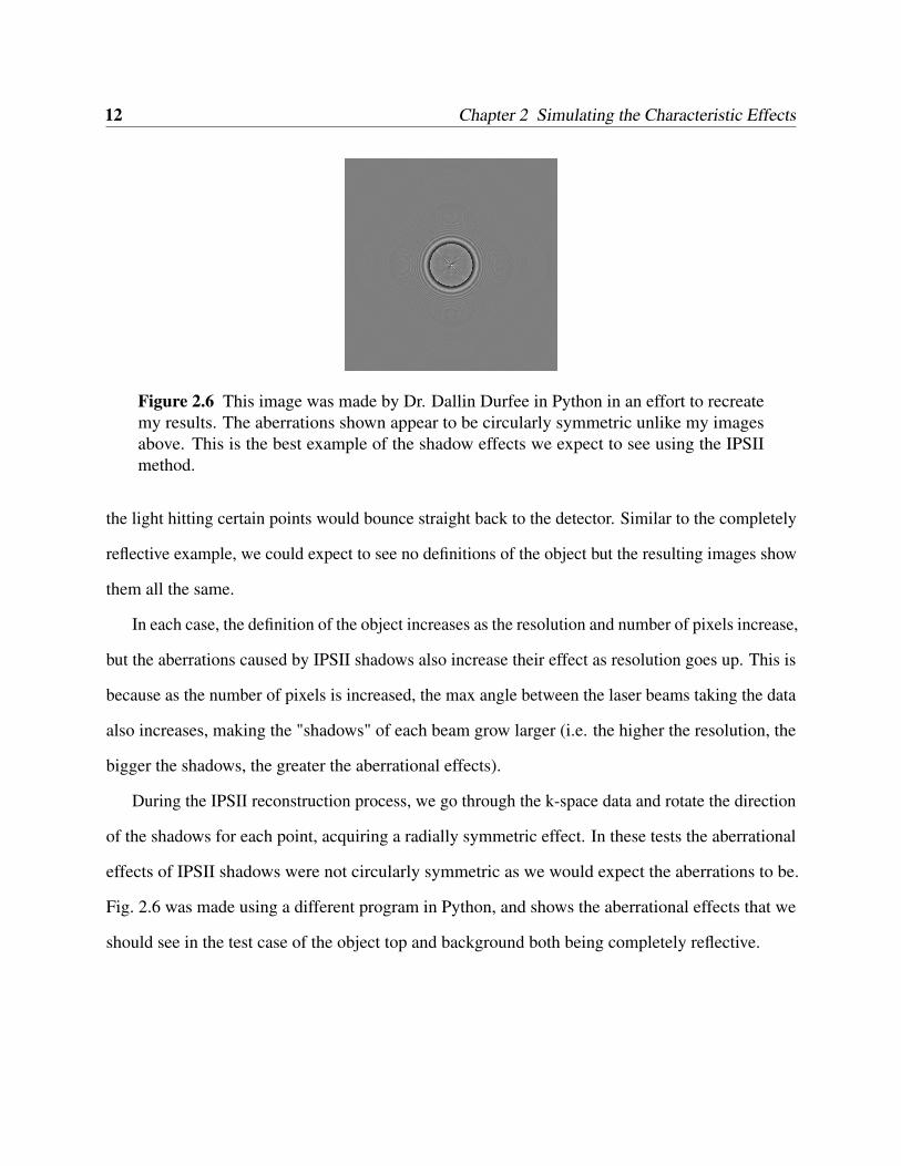
Figure 2.6 This image was made by Dr. Dallin Durfee in Python in an effort to recreatemy results. The aberrations shown appear to be circularly symmetric unlike my imagesabove. This is the best example of the shadow effects we expect to see using the IPSIImethod.

the light hitting certain points would bounce straight back to the detector. Similar to the completely

reflective example, we could expect to see no definitions of the object but the resulting images show

them all the same.

In each case, the definition of the object increases as the resolution and number of pixels increase,

but the aberrations caused by IPSII shadows also increase their effect as resolution goes up. This is

because as the number of pixels is increased, the max angle between the laser beams taking the data

also increases, making the "shadows" of each beam grow larger (i.e. the higher the resolution, the

bigger the shadows, the greater the aberrational effects).

During the IPSII reconstruction process, we go through the k-space data and rotate the direction

of the shadows for each point, acquiring a radially symmetric effect. In these tests the aberrational

effects of IPSII shadows were not circularly symmetric as we would expect the aberrations to be.

Fig. 2.6 was made using a different program in Python, and shows the aberrational effects that we

should see in the test case of the object top and background both being completely reflective.

Chapter 3

Experimental IPSII Shadows

Having simulated the IPSII process in Python and seen the aberrational effects the shadows had

on resulting images, the next step for me was to perform IPSII on objects with depth to verify our

computational results. This chapter describes my efforts to construct a working IPSII setup and

showcases the images we created with it.

3.1 Recreating IPSII

MAS-IPSII was designed by Jarom Jackson as a PhD project at BYU [4]. My research in that

same lab therefore focused on IPSII shadows using Python simulations and a MAS-IPSII setup and

design for experimental verification. I decided to replicate Dr. Jackson’s physical setup as exactly

as possible for my experiment to avoid any unnecessary nuances. Fig. 3.1 represents the kind of test

object he had imaged using his setup, and Fig. 3.2 contains some of his results. My goal was to first

achieve similar image results with my own setup, and then move on to imaging IPSII shadows.

13

14 Chapter 3 Experimental IPSII Shadows

(a) (b)

Figure 3.1 (a) Picture of a negative U.S. Air Force Resolution Test Target from Thorlabs[9] (1951 USAF Resolution Test Target (negative), Ø1"). Our lab used one just like it. (b)a zoomed in view of the pattern on the Test Target.

(a) (b) (c)

Figure 3.2 Taken from [4] (a,b) IPSII images of an Air Force test pattern made by Dr.Jarom Jackson during his PhD research. (c) example of good k-space data correspondingto an IPSII image

3.1 Recreating IPSII 15

Figure 3.3 Ramp signal to drive the piezo stack for phase scanning, 2.2 V at 5 Hz with90% symmetry

3.1.1 Setup

Using the design provided by Jarom Jackson (see Fig. 1.1b) Ben Whetten, a fellow undergraduate,

and I were able to setup the interferometer as hoped. Near the beginning, a lot my of time was spent

simply learning about all the parts and how they work. We glued a piezo stack to the back of a one

inch mirror placed in one of the bow tie configurations, and setup the controller to ramp the stack

signal for the phase scanning (see Fig. 3.3). To keep costs low, we used a low quality laser pointer

as our source, attenuated by a 10µm pinhole. The motorized mirror mounts were controlled by a

BeagleBone Black [10]. The reference and object signals were sent to a trans-impedance amplifier

connected to a Labjack T7 [11] which read the data and saved it to an external hard drive mounted

to the BeagleBone. I ran the experiment using Python [12]. The main body of the interferometer

can be seen in Fig. 3.4.

I balanced the interferometer (Fig. 3.4) as best I could so that each beam leg was equal in length.

It took me a while to set up the Labjack and BeagleBone to use Dr. Jackson’s code for run the

experiment autonomously. I also created a circuit for the Photo Multiplier Tube (PMT) [13] used

to read in the reference signal. For a while, we were were struggling to understand why the PMT

was not reading the expected signal, until we realized we needed to switch the polarity to negative.


Figure 3.4 Seen here is the setup we used for the experimental verification of IPSIIshadows, with the green lines representing the laser beam path(s).

After that, it worked well.

As I was about to start taking data, a power outage occurred that affected the lab, and there were

quite a few nuances to get everything back up and running again. My first successful images are

shown below.

3.1.2 Image Results

Using a pinhole and some aluminum foil to block out unnecessary light, I took an IPSII image of

an USAF test pattern (negative) like the one in Fig. 3.1. The Field of View (FOV) was set to be

500µm×500µm which was smaller than the exposed area of the test pattern. Fig. 3.5a shows the

resulting image. This run was the first successful one (it showed something resembling a part of the

test pattern), and appears to present a ghosting effect of the pattern lines. Fig. 3.5b shows almost

the same image, shifted, and with a slightly higher resolution.

We decided to try taking an image of the whole pattern to see how large of an FOV we could have

while still acquiring a reasonable image. Fig. 3.6 is an image of the test pattern with a 4mm×4mm


(a) (b)

Figure 3.5 (a) First run with channels correctly determined with 101×101 k-spacemeasurements and 500µm×500µm FOV. (b) Second run with correct channels. 151×151k-space measurements and 500µm×500µm FOV.

Figure 3.6 First IPSII run with no aperture before object. Also first run with 4mm×4mmFOV size of test pattern, and 301×301 k-space measurements.

FOV and a relatively high resolution. It shows lots of blurring where the outermost ring of lines

appears, and then goes into focus nearer the center. The effects of this blurring is due to phase errors

and is the subject of Ben Whetten’s undergraduate senior thesis [14].

Due to this relation and limit, we wanted to hone in on a more appropriate FOV for our images.

Also, to avoid getting aberrational effects from light beyond our FOV we taped aluminum foil over

the parts of the pattern found outside said FOV. Fig. 3.7 shows low resolution images with smaller

FOVs and aluminum foil blocking the rest of the pattern.


(a) (b)

Figure 3.7 (a) First run with aluminum foil as aperture. FOV 1mm×1mm, and 31×31k-space measurements. We should see the edges of the aluminum foil easily. (b) Secondtry with aluminum foil at low resolution. 41×41 k-space measurements and 2mm×2mmFOV.

Fig. 3.8a shows the same image as Fig. 3.7b taken at a much higher resolution, and we can see

that everything seems to be more blurred. It also shows the k-space data (Fig. 3.8b) of that image

and, as seen by the streaks and black space, that something caused the setup to stop taking data.

The cause of the black streaks and consequent lack of data for images like this was often a mirror

mount adjustment screw that disconnected in the middle of taking data. Upon gluing the screw back

together and reconnecting we attempted to take the image various times. Each subsequent time,

either the same or a different screw disconnected, probably from an excess of torque when adjusting

the mirrors. Once we took data and the screws stopped disconnecting, we found that the motors

were still not functioning properly. They would fail to return to physical home after movement

although they displayed digital home according to the computer. Upon switching out the motors and

trying again, the problem persisted, even though the code was the same as before when successfully

taking images of the test pattern.


(a) (b)

Figure 3.8 (a) IPSII image where something was off in the k-space data. (b) K-space dataof image. Parts of it show errors in the data, probably from a motor disconnecting from amirror mount.

Chapter 4

Conclusion

I was able to create simulated examples of the aberrational effects of IPSII shadows which, while

not creating the most accurate representation of the object being imaged, do provide some level of

object definition in the resulting image. When the reflectivity of the object and background are the

same, these shadow effects provide the only defining characteristics of the object in the image itself.

We failed to verify the effects of illumination shadows in IPSII experimentally, but were

successful in reconstructing the IPSII setup used by Jackson in [4], and partially successful in taking

images of an Air Force test pattern.

The next step to take involves successfully performing IPSII using a MAS-IPSII setup on an

object with significant axial extent.

21

22 Chapter 4 Conclusion

Appendix A

This appendix contains relevant code I made to simulate IPSII in Python. For the code used to

autonomously run our IPSII setup, see Dr. Jackson’s dissertation [4].

A.1 1D IPSII Simulation Code

This code is not exactly what was used, but is an accurate representation of the one-dimensional

simulation process as described in 2.1. It takes the Fourier transform (Eq. 2.1) of the Reflectivity

multiplied by a shadow mask, and then the resulting image is the inverse Fourier transform (ifft

here) of that result.

Python Code:

import numpy as np

R = ReflectivityN = len(R)FOV = FieldOfViewlmbda = wavelength

for n in range(N):dk = 1/FOVtheta = 2*np.arcsin(n*lmbda*dk/2)#apply shadow maskdata[n] = np.sum(R*np.exp(n*(-1j)*x*2*np.pi/N)*shadow)

23

24 Chapter A

image = np.fft.ifft(data)

A.2 2D IPSII Shadow Mask Code (POV-Ray)

I used version 3.8 of POV-Ray [8] from http://www.povray.org/. This code created an above-view

image of a cylinder and its shadows from two infinitely far away light sources at a specific angle

from each other. The angle between the light sources was determined by a given pixel number. The

number of pixels desired in the IPSII image determined the number of POV-Ray images I made

using this code.

POV-Ray Code:

#version 3.8;global_settings{ assumed_gamma 1.0 }

#declare l = 0.00532;#declare Angle = 0.006;#declare Camera_Distance = 20000;#declare deltakm = 1/( Camera_Distance*tan(Angle*pi /180));#declare deltakn = 1/( Camera_Distance*tan(Angle*pi /180));#declare theta = asin(l*sqrt(pow(m*deltakm ,2)+pow(n*deltakn ,2))/2);#declare phi = atan2(Nrow/2-m,n-Ncol /2);

#debug concat("\n", str(theta *180/pi ,1,3), "\n\n")

camera {orthographiclocation <0,Camera_Distance ,0>look_at <0,0,0>sky <0,0,1>angle Angle

}

light_source{<-cos(phi)*sin(theta),cos(theta),-sin(phi)*sin(theta)>*100000 color rgb 1 }

light_source{<cos(phi)*sin(theta),cos(theta),sin(phi)*sin(theta)>*100000 color rgb 1 }

http://www.povray.org/

A.3 2D IPSII Simulation Code 25

plane{ <0,1,0>, 0texture{ pigment { color rgb 1 }

finish { ambient 0 diffuse 1 }}

}

cylinder{<0,0,0>, <0,0.1,0>, 0.1texture{ pigment { color rgb <0,0,1> }

finish { ambient 0 diffuse 1 }}

}

A.3 2D IPSII Simulation Code

This is the code that was used to simulate the two-dimensional IPSII process as described in 2.2. It

takes the two-dimensional Fourier transform (Eq. 2.3) of the Reflectivity multiplied by a shadow

mask, and then the resulting image is the inverse Fourier transform (ifft2 here) of that result.

Python Code:

import numpy as npimport maplotlib.image as mpimg

######################################################################Forward Fourier transform function with shadow mask inside the

integrand#####################################################################

def transform_with_shadow(object_arr , reflectivity_arr , folder , size ,num_digits):Object = object_arrReflectivity = reflectivity_arr

Nrow = np.shape(Object)[0] # num rowsNcol = np.shape(Object)[1] # num columns

xr = range(Nrow)xc = range(Ncol)XC,XR = np.meshgrid(xc,xr)

26 Chapter A

integrand = np.empty(np.shape(Object), dtype=np.complex)IPSII = np.empty(np.shape(Object), dtype=np.complex)image_filepath = "/home/carter/Documents/Research/simple cylinder2/"+folder+"/shadows"

for m in range(size):for n in range(size):

shadow = mpimg.imread(image_filepath+'/m'+str(m+1).zfill(num_digits)+"/test"+str(m+1).zfill(num_digits)+str(n+1).zfill(num_digits)+".png")[:,:,0]

integrand = Reflectivity*np.exp((-1j)*2*np.pi*(m*XR/Nrow+ n*XC/Ncol))*shadow

IPSII[m,n] = sum(sum(integrand))

# theta = np.arcsin(l*np.sqrt (((m*deltakm)**2) +((n*deltakn)**2))/2)# phi = np.arctan ()

return IPSII

######################################################################Simulating IPSII with the forward transform , then taking the inverse

transform for the resulting image#####################################################################

IPSII128random = transform_with_shadow(gimg128 , randomgimg128 , "128x128", 128, 3)



plt.imshow(np.fft.ifft2(IPSII128random).real)plt.imshow(np.fft.ifft2(IPSII256random).real)plt.imshow(np.fft.ifft2(IPSII512random).real)

Appendix B

The original analysis program designed by Jarom Jackson used a sine fit method to create the images

from IPSII data. Later, I switched to using a lock-in amplification method that, while achieving

slightly more blurry images, was about ten times faster than Dr. Jackson’s sine fit program.

(a) (b)

Figure B.1 (a) Using a sin fit function to retrieve the phase and create the image. (b)Using lock-in detection to retrieve the phase and create the image.

27

28 Chapter B

(a) (b)

Figure B.2 (a) Using a sin fit function to retrieve the phase and create the image. (b)Using lock-in detection to retrieve the phase and create the image.

List of Figures

1.1 Rendering of Mach-Zehnder interferometer used for imaging . . . . . . . . . . . . 4

1.2 Example of Plane Wave Interference . . . . . . . . . . . . . . . . . . . . . . . . . 4

1.3 Basic Illustration of IPSII . . . . . . . . . . . . . . . . . . . . . . . . . . . . . . . 5

1.4 Example of Plane Wave Interference and Depth of Field . . . . . . . . . . . . . . . 5

1.5 Illustration of IPSII Shadows . . . . . . . . . . . . . . . . . . . . . . . . . . . . . 6

2.1 POV-Ray cylinder & mask . . . . . . . . . . . . . . . . . . . . . . . . . . . . . . 9

2.2 IPSII Simulation Height Map of Cylinder Object . . . . . . . . . . . . . . . . . . 10

2.3 IPSII Simulation of Cylinder Object (black on white) . . . . . . . . . . . . . . . . 10

2.4 IPSII Simulation of Cylinder Object (white on white) . . . . . . . . . . . . . . . . 11

2.5 IPSII Simulation of Cylinder Object (randomized reflectivity) . . . . . . . . . . . . 11

2.6 IPSII Simulation of Cylinder Object (circularly symmetric) . . . . . . . . . . . . . 12

3.1 USAF Test Pattern . . . . . . . . . . . . . . . . . . . . . . . . . . . . . . . . . . 14

3.2 IPSII Test Image . . . . . . . . . . . . . . . . . . . . . . . . . . . . . . . . . . . 14

3.3 Piezo ramp signal . . . . . . . . . . . . . . . . . . . . . . . . . . . . . . . . . . . 15

3.4 IPSII setup picture . . . . . . . . . . . . . . . . . . . . . . . . . . . . . . . . . . 16

3.5 Data Sets 014 & 015 . . . . . . . . . . . . . . . . . . . . . . . . . . . . . . . . . 17

3.6 Data Set 016 . . . . . . . . . . . . . . . . . . . . . . . . . . . . . . . . . . . . . . 17

29

30 LIST OF FIGURES

3.7 Data Sets 017 & 018 . . . . . . . . . . . . . . . . . . . . . . . . . . . . . . . . . 18

3.8 Data Set 020 . . . . . . . . . . . . . . . . . . . . . . . . . . . . . . . . . . . . . . 19

B.1 Data Set 014 (sine fit & lock-in) . . . . . . . . . . . . . . . . . . . . . . . . . . . 27

B.2 Data Set 015 (sine fit & lock-in) . . . . . . . . . . . . . . . . . . . . . . . . . . . 28

Bibliography

[1] D. Feldkhun and K. H. Wagner, “Doppler encoded excitation pattern tomographic optical

microscopy,” Appl. Opt. 49, H47–H63 (2010).

[2] J. J. Field, D. G. Winters, and R. A. Bartels, “Plane wave analysis of coherent holographic

image reconstruction by phase transfer (CHIRPT),” J. Opt. Soc. Am. A 32, 2156–2168 (2015).

[3] B. Judkewitz and C. Yang, “Axial standing-wave illumination frequency-domain imaging

(SWIF),” Opt. Express 22, 11001–11010 (2014).

[4] J. S. Jackson, PhD dissertation, Brigham Young University, 2019.

[5] J. Jackson and D. Durfee, “Demonstration of Interference Pattern Structured Illumination

Imaging,” In Frontiers in Optics / Laser Science, Frontiers in Optics p. FW7B.6 (Optical

Society of America, 2018).

[6] J. Jackson and D. Durfee, “Lensless Single Pixel Imaging with Laser Interference Patterns,”

Microscopy and Microanalysis 24, 1366–1367 (2018).

[7] J. Jackson and D. Durfee, “Mechanically scanned interference pattern structured illumination

imaging,” Optics Express 27, 14969–14980 (2019).

[8] P. of Vision Raytracer Pty. Ltd., Persistence of Vision Raytracer, 2013 (accessed June 8, 2020).

[9] I. Thorlabs, Thorlabs, 2020 (accessed June 8, 2020).31

32 BIBLIOGRAPHY

[10] BeagleBone, BeagleBone Black System Reference Manual, 2014, rev. C.1.

[11] LabJack, T-Series Datasheet, 2020, something good.

[12] P. S. Foundation, Python, 2020 (accessed June 8, 2020).

[13] HAMAMATSU, 931B Photomultiplier Tube Technical Data Sheet.

[14] B. Whetten, undergraduate thesis, Brigham Young University, 2020.