Effective slippage on superhydrophobic trapezoidal groovesJiajia Zhou, Evgeny S. Asmolov, Friederike Schmid, and Olga I. Vinogradova

Citation: The Journal of Chemical Physics 139, 174708 (2013); doi: 10.1063/1.4827867 View online: http://dx.doi.org/10.1063/1.4827867 View Table of Contents: http://scitation.aip.org/content/aip/journal/jcp/139/17?ver=pdfcov Published by the AIP Publishing Articles you may be interested in Lattice-Boltzmann simulations of the drag force on a sphere approaching a superhydrophobic striped plane J. Chem. Phys. 140, 034707 (2014); 10.1063/1.4861896 A numerical study of the effects of superhydrophobic surface on skin-friction drag in turbulent channel flow Phys. Fluids 25, 110815 (2013); 10.1063/1.4819144 Scaling laws for slippage on superhydrophobic fractal surfaces Phys. Fluids 24, 012001 (2012); 10.1063/1.3674300 On the effects of liquid-gas interfacial shear on slip flow through a parallel-plate channel with superhydrophobicgrooved walls Phys. Fluids 22, 102002 (2010); 10.1063/1.3493641 Intrinsic slip on hydrophobic self-assembled monolayer coatings Phys. Fluids 22, 042003 (2010); 10.1063/1.3394120

This article is copyrighted as indicated in the article. Reuse of AIP content is subject to the terms at: http://scitation.aip.org/termsconditions. Downloaded to IP:

31.148.218.97 On: Tue, 29 Apr 2014 17:56:57

THE JOURNAL OF CHEMICAL PHYSICS 139, 174708 (2013)

Effective slippage on superhydrophobic trapezoidal groovesJiajia Zhou,1 Evgeny S. Asmolov,2,3,4 Friederike Schmid,1 and Olga I. Vinogradova2,5,6

1Institut für Physik, Johannes Gutenberg-Universität Mainz, D55099 Mainz, Germany2A.N. Frumkin Institute of Physical Chemistry and Electrochemistry, Russian Academy of Science,31 Leninsky Prospect, 119071 Moscow, Russia3Central Aero-Hydrodynamic Institute, 140180 Zhukovsky, Moscow Region, Russia4Institute of Mechanics, M.V. Lomonosov Moscow State University, 119991 Moscow, Russia5Department of Physics, M.V. Lomonosov Moscow State University, 119991 Moscow, Russia6DWI, RWTH Aachen, Forckenbeckstraße 50, 52056 Aachen, Germany

(Received 19 August 2013; accepted 17 October 2013; published online 6 November 2013)

We study the effective slippage on superhydrophobic grooves with trapezoidal cross-sections of var-ious geometries (including the limiting cases of triangles and rectangular stripes), by using twocomplementary approaches. First, dissipative particle dynamics (DPD) simulations of a flow pastsuch surfaces have been performed to validate an expression [E. S. Asmolov and O. I. Vinogradova,J. Fluid Mech. 706, 108 (2012)] that relates the eigenvalues of the effective slip-length tensor forone-dimensional textures. Second, we propose theoretical estimates for the effective slip length andcalculate it numerically by solving the Stokes equation based on a collocation method. The com-parison between the two approaches shows that they are in excellent agreement. Our results demon-strate that the effective slippage depends strongly on the area-averaged slip, the amplitude of theroughness, and on the fraction of solid in contact with the liquid. To interpret these results, we ana-lyze flow singularities near slipping heterogeneities, and demonstrate that they inhibit the effectiveslip and enhance the anisotropy of the flow. Finally, we propose some guidelines to design optimalone-dimensional superhydrophobic surfaces, motivated by potential applications in microfluidics.© 2013 AIP Publishing LLC. [http://dx.doi.org/10.1063/1.4827867]

I. INTRODUCTION

The design and fabrication of micro- and nanotexturedsurfaces has received much attention during the past decade.In case of a hydrophobic texture, a modified surface profilecan lead to a very large contact angle, which induces excep-tional wetting properties.1 A remarkable mobility of liquidson such superhydrophobic surfaces is observed in the Cassiestate, where the textures are filled with gas, which rendersthem “self-cleaning” and causes droplets to roll (rather thanslide) under gravity2 and rebound (rather than spread) uponimpact.3, 4 Furthermore, patterned superhydrophobic materi-als are important in context of fluid dynamics and their su-perlubricating properties.5, 6 In particular, superhydrophobicheterogeneous surfaces in the Cassie state exhibit very lowfriction, and this drag reduction is associated with the largeslippage of liquids.7–9

It is very difficult to quantify the flow past heteroge-neous surfaces. However, analytical results can often be ob-tained using an effective slip boundary condition, beff, at theimaginary smooth homogeneous, but generally anisotropicsurface.9, 10 For anisotropic textures, the effective slip gener-ally depends on the direction of the flow and is a tensor, beff

≡ {beffij } represented by a symmetric, positive definite 2 × 2

matrix,11

beff = Sθ

(b

‖eff 0

0 b⊥eff

)S−θ , (1)

diagonalized by a rotation

Sθ =(

cos θ sin θ

− sin θ cos θ

). (2)

Equation (1) allows us to calculate an effective slip in anydirection given by an angle θ , provided the two eigenvaluesof the slip-length tensor, b

‖eff (θ = 0) and b⊥

eff (θ = π /2), areknown. The concept of an effective slip length tensor is gen-eral and can be applied for arbitrary channel thickness.12 It isa global characteristic of a channel,9 and the eigenvalues usu-ally depend not only on the parameters of the heterogeneoussurfaces, but also on the channel thickness. However, for athick channel (compared to a texture period, L) they becomea characteristic of a heterogeneous interface solely.

An important type of such surfaces are highly anisotropictextures, where a (scalar) partial local slip b(y) varies in onlyone direction. Such surfaces can be created experimentally bymaking textured surfaces with one dimensional surface pro-files, and in the Cassie state, the local slip length will alwaysreflect the relief of the texture. This is the consequence of the“gas cushion model,” which takes into account that the dissi-pation at the gas/liquid interface is dominated by the shearingof a continuous gas layer,13, 14

b(y) � μ

μg

e(y), (3)

where μg and μ are dynamic viscosities of a gas and a liquid,and e is the thickness of the gas layer. Equation (3) repre-sents an upper bound for a local slip at the gas area, which is

0021-9606/2013/139(17)/174708/11/$30.00 © 2013 AIP Publishing LLC139, 174708-1

This article is copyrighted as indicated in the article. Reuse of AIP content is subject to the terms at: http://scitation.aip.org/termsconditions. Downloaded to IP:

31.148.218.97 On: Tue, 29 Apr 2014 17:56:57

174708-2 Zhou et al. J. Chem. Phys. 139, 174708 (2013)

attained in the limit of a small fraction of the solid phase.At a relatively large solid fraction15 or if the flux in the“pockets” of superhydrophobic surfaces is equal to zero,16, 17

Eq. (3) could overestimate the local slip. However, even in allsituations the local slip length profile, b(y), necessarily fol-lows the relief of the texture provided it is shallow enough,e(y) � L.17 Since in case of water Eq. (3) leads to b(y)� 50e(y), it is expected that the “gas cushion model” couldbe safely applied up to b(y)/L = O(10) or so.

The flow properties on highly anisotropic surfaces can behighly peculiar. In particular, off-diagonal effects may be ob-tained where a driving force (such as pressure gradient, shearrate, or electric field) in one direction induces a flow in a dif-ferent direction, with a measurable and useful perpendicularcomponent. This could be exploited for implementing trans-verse pumps, mixers, flow detectors, and more.18, 19 The maintask is to find the connection between the eigenvalues of theslip-length tensor and the parameters of such one-dimensionalsurface textures. Up to now analytical results for the effectiveslip length have only been obtained for the simplest geometryof rectangular grooves.12, 20–24 We are unaware of any priorwork that has obtained analytical results for other types ofone-dimensional textures.

However, some recently derived relations for the caseof an anisotropic isolated surface (corresponding to the thickchannel limit) allow one to simplify the analysis of more com-plex geometries, and to rationalize the limiting behavior of theeffective slip length in certain regimes. We mention first thatthe transverse component of the slip-length tensor was pre-dicted to be exactly half the longitudinal component that onewould obtain if the local slip were multiplied with a factortwo, 2b(y),25

b⊥eff

[b (y) /L

] = b‖eff

[2b (y) /L

]2

. (4)

This relation can greatly simplify the analysis since it indi-cates that the flow along any direction of the one-dimensionalsurface can be easily determined, once the longitudinal com-ponent of the effective slip tensor is found. Equation (4)has been recently verified for a texture with sinusoidal su-perhydrophobic grooves by using a Lattice Boltzmann (LB)method,26 and for weakly slipping stripes by using dissipativeparticle dynamics (DPD) simulations.24

Another useful relation addresses the particular casewhere the local slip is large, b(y)/L � 1. In that case, the ef-fective slip length tensor beff becomes isotropic and is givenby26, 27

b‖eff � b⊥

eff �⟨

1

b(y)

⟩−1

, (5)

where 〈1/b(y)〉 is the mean inverse local slip. Finally, forweakly slipping patterns with b(y)/L � 1, the flow again be-comes isotropic, and its value is equal to the surface averageof the local slip length,10, 21

b‖eff � b⊥

eff � 〈b(y)〉 = 〈b〉. (6)

Note that Eq. (6) is expected to be accurate for a continuouslocal slip profile only. If the local slip length exhibits step-likejumps at the edges of heterogeneities, the expansions leading

to Eq. (6) become questionable. Higher order contributions tothe effective slip become comparable to the first-order termgiven by Eq. (6) and can no longer be ignored.24

Computer simulations and numerical modeling can shedlight on flow phenomena past one-dimensional surfaces. Inefforts to better understand the connection between the pa-rameters of the texture and the effective slip lengths, severalgroups have performed continuum and Molecular Dynamicssimulations of flow past anisotropic surfaces. Most of thesestudies focused on calculating eigenvalues of the effectiveslip-length tensor for superhydrophobic stripes.28–30 To studyvarious aspects of a flow past striped walls, recent works em-ployed Dissipative particle dynamics (DPD)23, 24, 31 and Lat-tice Boltzmann (LB)12 methods. In the case of stripes with apiecewise constant local slip profile (i.e., the profile featuressteplike jumps at the boundaries of the stripes), the singularityin the slip profile induces singularities both in the pressure andvelocity gradient, which generates an additional mechanismfor dissipation even at small local slip.24, 25 Anisotropic one-dimensional texture with continuously varying patterns canproduce a very large effective slip. This has been confirmedin recent LB simulations studies of sinusoidal textures.26 One-dimensional continuous surfaces may also exhibit singulari-ties (for example, the first derivative may be discontinuous).However, we are unaware of any previous work that has ad-dressed the question of effective slip lengths past such tex-tures.

In this paper, we study the friction properties on trape-zoidal superhydrophobic grooves [see Fig. 1(a)]. This textureis more general than rectangular grooves since it providesan additional geometrical structure parameter, i.e., the trape-zoid base width. Also, the trapezoid texture can be extendedto its extremes, such as a triangular patterns, where the liq-uid/solid contact area vanishes, and rectangular reliefs. Su-perhydrophobic trapezoidal textures were shown to give largecontact angles, and to provide stable Cassie states.32 An obvi-ous advantage of the trapezoidal surface relief is that the man-ufactured texture becomes mechanically more stable againstbending compared to rectangular grooves. Furthermore, it canbe naturally formed from dilute rectangular grooves as a re-sult of elasto-capillarity.33 This type of surfaces has alreadybeen intensively used in slippage experiments.34 However, theimpact of trapezoidal texture reliefs on transport and hydro-dynamic slippage remains largely unknown.

Our study is based on the use of DPD simulations,which we have put forward in our previous papers,23, 24 onthe numerical solution of the Stokes equations (a collocationmethod), and on theoretical analysis. In particular, we vali-date Eq. (4) for trapezoidal textures with various parameters,we apply Eq. (5) to evaluate an effective slip for strongly slip-ping patterns, we discuss the singularities in velocities causedby inflection points in the local slip profiles, which in particu-lar lead to deviations from Eq. (6), and we finally suggest theoptimal design of trapezoidal patterns.

II. MODEL AND GOVERNING EQUATIONS

We consider creeping flow along a plane anisotropicsuperhydrophobic wall, using a Cartesian coordinate

This article is copyrighted as indicated in the article. Reuse of AIP content is subject to the terms at: http://scitation.aip.org/termsconditions. Downloaded to IP:

31.148.218.97 On: Tue, 29 Apr 2014 17:56:57

174708-3 Zhou et al. J. Chem. Phys. 139, 174708 (2013)

φ1L φ2Lb2

b1 y

b

e

L

x y

z

θ

(a)

(b)

<b>

FIG. 1. Sketch of the trapezoidal superhydrophobic surface in the Cassiestate (a), and, according to Eq. (3), of the corresponding local slip length (b).

system (x, y, z) (Fig. 1). As in most previouspublications,7, 12, 15, 20, 29, 35–37 we model the superhydrophobicplate as a flat heterogeneous interface. In such a descrip-tion, we neglect an additional mechanism for a dissipationconnected with the meniscus curvature.15, 38, 39 Note howeverthat such an ideal situation has been achieved in many recentexperiments.40–42 The origin of coordinates is placed at theflat interface, characterized by a slip length b(y), spatiallyvarying in one direction, and the texture varies over aperiod L.

The local slip length is taken to be a piecewise linearfunction. It includes two regions with a constant slip: onewhere the slip length assumes its minimum value, b1, whichhas area fraction of φ1, and another with area fraction φ2

where the slip length is maximal. These regions are connectedby two transition regions with equal surface fractions (1 − φ1

− φ2)/2, where the local slip length varies linearly from b1

to b2. If we rewrite the coordinate y in the form y = (n + t)L,where n is an integer number and |t | ≤ 1

2 , the local slip-lengthprofile can be expressed in terms of t:

b(y) =

⎧⎪⎪⎨⎪⎪⎩

b1, |t | ≤ φ1

2

b1 + 2(b2−b1)1−φ1−φ2

(|t | − φ1

2

),

φ1

2 < |t | ≤ 1−φ2

2

b2,1−φ2

2 < |t | ≤ 12

. (7)

For φ1 = φ2 = 0, we get a triangular profile

b(y) = b1 + 2(b2 − b1)|t |, |t | ≤ 1

2. (8)

Note that regular trapezoidal and triangular profiles are con-tinuous functions (albeit with a discontinuous first derivative).However, in the limit φ1 + φ2 = 1, the profile reduces tothe discontinuous rectangular slip length profile (alternatingstripe profile) studied in earlier work,

b(y) ={

b1, |t | ≤ φ1

2

b2,φ1

2 < |t | ≤ 12

. (9)

Our results apply to a single surface in a thick chan-nel, where effective hydrodynamic slip is determined by flowat the scale of roughness, so that the velocity profile suffi-ciently far above the surface may be considered as a linear

shear flow.7, 9 However, it does not apply to a thin37 or anarbitrary12 channel situation, where the effective slip scaleswith the channel width. Note that the flow in thin channelswith superhydrophobic trapezoidal textures has been consid-ered in recent work.17

Dimensionless variables are defined by using L as a ref-erence length scale, the inverse shear rate 1/G sufficientlyfar from the surface as a reference time. At small Reynoldsnumber, Re = GL2/ν, the dimensionless velocity and pressurefields, v and p, satisfy Stokes equations

∇ · v = 0,

(10)∇p − �v = 0.

Due to Eq. (4), it is sufficient to consider the flow parallelto the pattern (x-axis). In this case, the velocity has only onecomponent in the x-direction v = (v(y, z), 0, 0), and we seeka solution for the velocity profile of the form

v = U + u, (11)

where U = z is the undisturbed linear shear flow. The pertur-bation of the flow, u(y, z), which is caused by the presence ofthe texture and decays far from the interface. It follows fromStokes’ equations that ∂yp = ∂zp = 0. Since the pressure isconstant far from the superhydrophobic surface this impliesthat it also remains constant in the entire flow region. The ve-locity perturbation satisfies a dimensionless Laplace equation,

�u = 0. (12)

The boundary conditions at the wall and at infinity are definedin the usual way,

z = 0 : u − b(y)

L∂zu = b(y)

L, (13)

z → ∞ : ∂zu = 0. (14)

The general solution to Eq. (12), decaying at infinity, canbe represented in terms of a cosine Fourier series as

u = a0

2+

∞∑n=1

an exp(−2πnz) cos(2πny), (15)

where an are coefficients to be found by applying the appro-priate boundary condition (13). It can be written in terms ofthe Fourier coefficients as

a0

2+

∞∑n=1

[1 + 2πn

b(y)

L(y)

]an cos (2πny) = b(y)

L. (16)

Equation (16) was used to determine the longitudinal effec-tive slip numerically. This was done using a method similar toRef. 24. We truncate the sum in Eq. (16) at some cut-off number N (usually N = 1001) and evaluate it in thepoints yl = l/2(N − 1), where l are numbers varyingfrom 0 to N − 1. The problem is then reduced to a lin-ear system of equations, Al

nanL = bl, where Al

0 = 1/2; Aln

= [1 + 2πnb(yl)/L] cos(2πnyl), n > 0 and bl = b(yl). The

This article is copyrighted as indicated in the article. Reuse of AIP content is subject to the terms at: http://scitation.aip.org/termsconditions. Downloaded to IP:

31.148.218.97 On: Tue, 29 Apr 2014 17:56:57

174708-4 Zhou et al. J. Chem. Phys. 139, 174708 (2013)

system is solved using the IMSL routine LSARG. The trans-verse effective slip was then calculated using Eq. (4).

III. DISSIPATIVE PARTICLE DYNAMICS SIMULATION

Mesoscale fluid simulations were performed using thedissipative particle dynamics (DPD) method.43–45 Morespecifically, we use a version of DPD without conservativeinteractions46 and combine that with a tunable-slip method47

to model patterned surfaces. The tunable-slip method allowsone to implement arbitrary hydrodynamic boundary condi-tion in coarse-grained simulations. In the following, we givea brief description of the model and introduce the implemen-tation of planar surfaces with arbitrary one-dimensional slipprofile.

The basic DPD equations involve pair interactions be-tween fluid particles. The pair forces are equal in magnitudebut opposite in direction; thus the momentum is conserved forthe whole system. This leads to the correct long-time hydro-dynamic behavior (i.e., Navier-Stokes). The pair force con-sists of a dissipative contribution and a random component,

FDPDij = FD

ij + FRij . (17)

The dissipative part FDij is proportional to the relative velocity

between two particles vij = vi − vj ,

FDij = −γDPD ωD(rij )(vij · r̂ij )r̂ij , (18)

with a local distance-dependent friction coefficient γ DPDωD

(rij). The weight function ωD(rij) is a monotonically decreas-ing function of rij and vanishes at a given cutoff, and γ DPD isa parameter that controls the strength of the dissipation. Therandom force FR

ij has the form

FRij = √

2kBT γDPD ωD(rij )ξij r̂ij , (19)

where ξ ij = ξ ji is a symmetric random number with a zeromean and a unit variance. The amplitude of the stochas-tic contribution is related to the dissipative contribution bya fluctuation-dissipation theorem in order to ensure that themodel reproduces the correct equilibrium distribution.

The tunable-slip method47 introduces the wall interactionin a similar fashion. The force exerted by the wall on particlei is given by

Fwalli = FWCA

i + FDi + FR

i . (20)

The first term is a repulsive interaction that prevents the fluidparticles from penetrating the wall. It can be written in termof the gradient of a Weeks-Chandler-Andersen potential,48

FWCAi = −∇V (z),

V (z) ={

4ε[(

σz

)12 − (σz

)6 + 14

]z <

6√

2 σ

0 z ≥ 6√

2 σ, (21)

where z is the distance between the fluid particle and the wall,assuming the wall lies in xy plane, and ε and σ set the energyand length scales. In the following, physical quantities will bereported in a model unit system of σ (length), m (mass), andε (energy). The dissipative contribution is similar to Eq. (18),

with the velocity replaced by the relative particle velocity withrespect to the wall. For immobile walls, the dissipative partcan be written as

FDi = −γLωL(z)vi . (22)

The parameter γ L characterizes the strength of the wall fric-tion and can be used to tune the value of the slip length. Forexample, γ L = 0 results in a perfectly slippery wall, whereasa positive value of γ L leads to a finite slip length. The randomforce has the form

FRi =

√2kBT γLωL(z)ξ i , (23)

where each component of ξ i is a random variable. Again,the magnitude of the random force is chosen such that thefluctuation-dissipation theorem is satisfied.

For homogeneous surfaces, a useful analytical expres-sion can be derived which establishes a relation between theslip length b and the simulation parameters (the wall frictionparameter γ L and the cutoff rc) to a good approximation.47

However, the accuracy of the analytic result is not satisfac-tory at small slip lengths. For the purpose of the present work,we need an accurate expression for the relation between theslip length and the tuning parameter γ L. Therefore, we havesimulated plane Poiseuille and Couette flows with differentγ L to obtain the slip length and the position of the hydrody-namic boundary. The simulation results were fitted to a trun-cated Laurent series up to second order in γ L and first orderin 1/γ L. The simulation data and the fitted curve are shown inFig. 2. The fit yields the expression

b = 1.498

γL− 0.3291 + 0.01457γL − 0.001101γ 2

L . (24)

This formula relates the wall friction coefficient γ L, whichis set in the simulation, to the slip length b. Also shown inFig. 2 is the analytic result in dashed line, which agrees withthe simulation data quite well at large slip length.

One important observation is that both the slip length band the friction coefficient γ L are local quantities. Thus, itis reasonable to assume that the relation (24) also holds for

-50

0

50

100

150

200

250

300

350

0.01 0.1 1 10

b [σ

]

γL [(mε)1/2/σ]

-1012345

0 1 2 3 4 5 6 7 8 9 10

FIG. 2. The relation between the slip length b and the wall friction coefficientγ L, for a wall interaction cutoff 2.0σ . The inset shows an enlarged portionof the region where the slip length is close to zero. The no-slip boundarycondition is implemented by using γL = 5.26

√mε/σ . The solid lines are the

fitting result Eq. (24), and the dashed curves show the analytical prediction.

This article is copyrighted as indicated in the article. Reuse of AIP content is subject to the terms at: http://scitation.aip.org/termsconditions. Downloaded to IP:

31.148.218.97 On: Tue, 29 Apr 2014 17:56:57

174708-5 Zhou et al. J. Chem. Phys. 139, 174708 (2013)

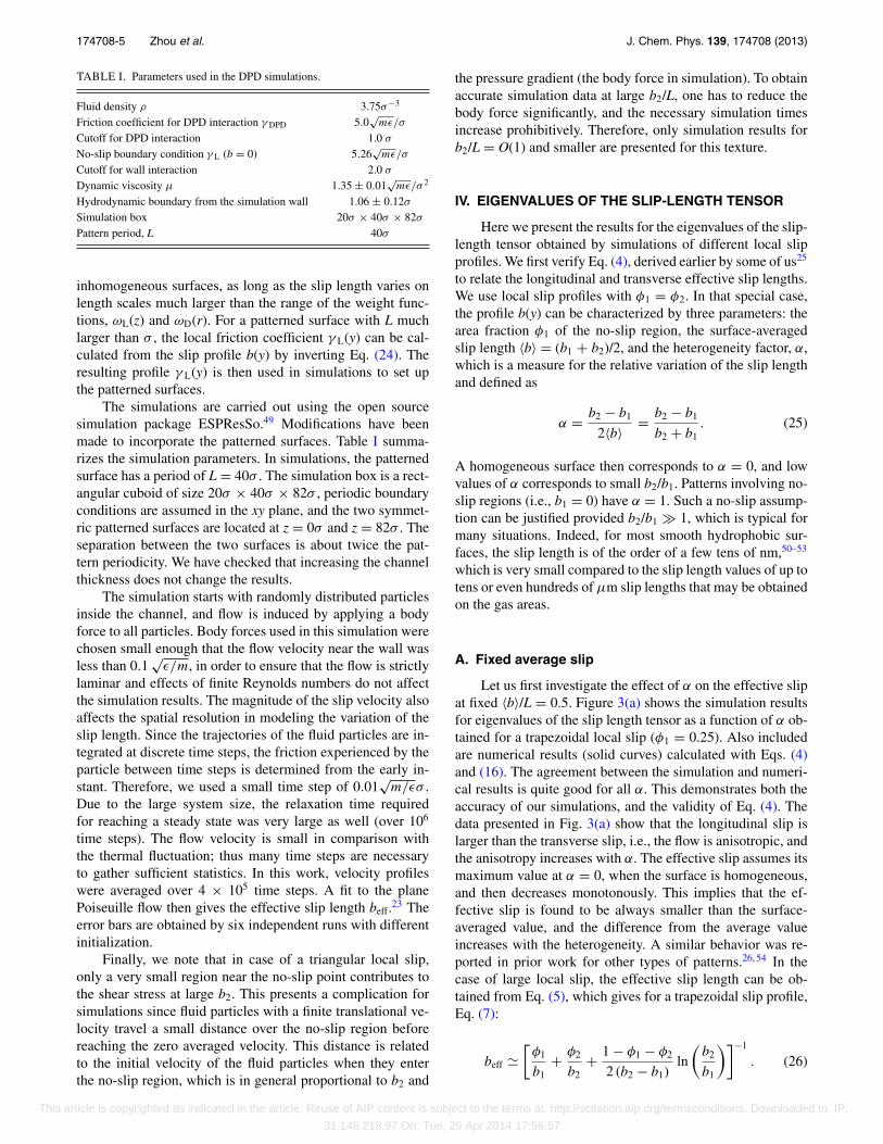
TABLE I. Parameters used in the DPD simulations.

Fluid density ρ 3.75σ−3

Friction coefficient for DPD interaction γ DPD 5.0√

mε/σ

Cutoff for DPD interaction 1.0 σ

No-slip boundary condition γ L (b = 0) 5.26√

mε/σ

Cutoff for wall interaction 2.0 σ

Dynamic viscosity μ 1.35 ± 0.01√

mε/σ 2

Hydrodynamic boundary from the simulation wall 1.06 ± 0.12σ

Simulation box 20σ × 40σ × 82σ

Pattern period, L 40σ

inhomogeneous surfaces, as long as the slip length varies onlength scales much larger than the range of the weight func-tions, ωL(z) and ωD(r). For a patterned surface with L muchlarger than σ , the local friction coefficient γ L(y) can be cal-culated from the slip profile b(y) by inverting Eq. (24). Theresulting profile γ L(y) is then used in simulations to set upthe patterned surfaces.

The simulations are carried out using the open sourcesimulation package ESPResSo.49 Modifications have beenmade to incorporate the patterned surfaces. Table I summa-rizes the simulation parameters. In simulations, the patternedsurface has a period of L = 40σ . The simulation box is a rect-angular cuboid of size 20σ × 40σ × 82σ , periodic boundaryconditions are assumed in the xy plane, and the two symmet-ric patterned surfaces are located at z = 0σ and z = 82σ . Theseparation between the two surfaces is about twice the pat-tern periodicity. We have checked that increasing the channelthickness does not change the results.

The simulation starts with randomly distributed particlesinside the channel, and flow is induced by applying a bodyforce to all particles. Body forces used in this simulation werechosen small enough that the flow velocity near the wall wasless than 0.1

√ε/m, in order to ensure that the flow is strictly

laminar and effects of finite Reynolds numbers do not affectthe simulation results. The magnitude of the slip velocity alsoaffects the spatial resolution in modeling the variation of theslip length. Since the trajectories of the fluid particles are in-tegrated at discrete time steps, the friction experienced by theparticle between time steps is determined from the early in-stant. Therefore, we used a small time step of 0.01

√m/εσ .

Due to the large system size, the relaxation time requiredfor reaching a steady state was very large as well (over 106

time steps). The flow velocity is small in comparison withthe thermal fluctuation; thus many time steps are necessaryto gather sufficient statistics. In this work, velocity profileswere averaged over 4 × 105 time steps. A fit to the planePoiseuille flow then gives the effective slip length beff.23 Theerror bars are obtained by six independent runs with differentinitialization.

Finally, we note that in case of a triangular local slip,only a very small region near the no-slip point contributes tothe shear stress at large b2. This presents a complication forsimulations since fluid particles with a finite translational ve-locity travel a small distance over the no-slip region beforereaching the zero averaged velocity. This distance is relatedto the initial velocity of the fluid particles when they enterthe no-slip region, which is in general proportional to b2 and

the pressure gradient (the body force in simulation). To obtainaccurate simulation data at large b2/L, one has to reduce thebody force significantly, and the necessary simulation timesincrease prohibitively. Therefore, only simulation results forb2/L = O(1) and smaller are presented for this texture.

IV. EIGENVALUES OF THE SLIP-LENGTH TENSOR

Here we present the results for the eigenvalues of the slip-length tensor obtained by simulations of different local slipprofiles. We first verify Eq. (4), derived earlier by some of us25

to relate the longitudinal and transverse effective slip lengths.We use local slip profiles with φ1 = φ2. In that special case,the profile b(y) can be characterized by three parameters: thearea fraction φ1 of the no-slip region, the surface-averagedslip length 〈b〉 = (b1 + b2)/2, and the heterogeneity factor, α,which is a measure for the relative variation of the slip lengthand defined as

α = b2 − b1

2〈b〉 = b2 − b1

b2 + b1. (25)

A homogeneous surface then corresponds to α = 0, and lowvalues of α corresponds to small b2/b1. Patterns involving no-slip regions (i.e., b1 = 0) have α = 1. Such a no-slip assump-tion can be justified provided b2/b1 � 1, which is typical formany situations. Indeed, for most smooth hydrophobic sur-faces, the slip length is of the order of a few tens of nm,50–53

which is very small compared to the slip length values of up totens or even hundreds of μm slip lengths that may be obtainedon the gas areas.

A. Fixed average slip

Let us first investigate the effect of α on the effective slipat fixed 〈b〉/L = 0.5. Figure 3(a) shows the simulation resultsfor eigenvalues of the slip length tensor as a function of α ob-tained for a trapezoidal local slip (φ1 = 0.25). Also includedare numerical results (solid curves) calculated with Eqs. (4)and (16). The agreement between the simulation and numeri-cal results is quite good for all α. This demonstrates both theaccuracy of our simulations, and the validity of Eq. (4). Thedata presented in Fig. 3(a) show that the longitudinal slip islarger than the transverse slip, i.e., the flow is anisotropic, andthe anisotropy increases with α. The effective slip assumes itsmaximum value at α = 0, when the surface is homogeneous,and then decreases monotonously. This implies that the ef-fective slip is found to be always smaller than the surface-averaged value, and the difference from the average valueincreases with the heterogeneity. A similar behavior was re-ported in prior work for other types of patterns.26, 54 In thecase of large local slip, the effective slip length can be ob-tained from Eq. (5), which gives for a trapezoidal slip profile,Eq. (7):

beff �[φ1

b1+ φ2

b2+ 1 − φ1 − φ2

2 (b2 − b1)ln

(b2

b1

)]−1

. (26)

This article is copyrighted as indicated in the article. Reuse of AIP content is subject to the terms at: http://scitation.aip.org/termsconditions. Downloaded to IP:

31.148.218.97 On: Tue, 29 Apr 2014 17:56:57

174708-6 Zhou et al. J. Chem. Phys. 139, 174708 (2013)

0.00

0.10

0.20

0.30

0.40

0.50

0.60

0 0.2 0.4 0.6 0.8 1

b eff/

L

α

(a)(a)

0.10

0.20

0.30

0.40

0.50

0 0.2 0.4 0.6 0.8 1

b eff/

L

α

(b)(b)(b)(b)

FIG. 3. (a) Longitudinal (open symbols) and transverse (closed symbols) ef-fective slip for a trapezoidal texture with an average slip 〈b〉/L = 0.5. Solidcurves show corresponding numerical solutions. Dash-dotted curve showsasymptotic solution in the limit of the large local slip [Eq. (26)]. (b) Lon-gitudinal effective slip length simulated (from top to bottom) for triangular,trapezoidal, and rectangular profiles with the same average slip 〈b〉/L = 0.5(symbols) and corresponding numerical data.

Figure 3(a) includes the theoretical curve expected forthis (isotropic) case (dash-dotted line). We note that the sliplength is always smaller than the average slip, 〈b〉/L = 0.5.Perhaps the most interesting and important result here is thatEq. (26) remains surprisingly accurate even in the case ofmoderate, but not vanishing, local slip, provided α is smallenough. We remind the reader that Eq. (26) may not be usedwhen α = 1, i.e., for textures with no-slip regions, b1 = 0,where it would simply predicts the effective slip length to bezero.

Qualitatively similar results were obtained for rectan-gular stripes and triangular local slip profiles. Therefore wedo not show these results here. We only recall that in thecase of stripes, the asymptotic result for large slip gives (seeRefs. 26 and 28 for the original derivations),

beff �[φ1

b1+ φ2

b2

]−1

, (27)

and for triangular profiles, one can derive

beff � 2(b2 − b1)

ln(b2/b1). (28)

To examine the difference between the different slip pro-files, the results for a longitudinal effective slip for a tex-ture with a trapezoidal local slip from Fig. 3(a) are repro-duced in Fig. 3(b). Also included in Fig. 3(b) are numericaland simulation data for rectangular (φ1 = 0.5) and triangular(φ1 = 0) profiles with the same average slip. The data showthat the triangular profile gives a larger, and the rectangularone a smaller effective slip than that resulting from the trape-zoidal local slip. We note that φ1 is very different for theseslip-length profiles. This suggests that one of the key parame-ters determining the effective slip is the area fraction of solidin contact with the liquid. If it is very small, the effective sliplength becomes large. Another important factor is the pres-ence of flow singularities near slipping heterogeneities as wewill discuss below.

B. Fixed heterogeneity factor

We now fix α = 1 and consider flows that are maxi-mally anisotropic for a given pattern, which corresponds tob1 = 0 (no-slip areas) and b2 = 2〈b〉. It is instructive to fo-cus first on the role of b2. Figure 4 shows the eigenvalues ofthe slip-length tensor as a function of b2/L as obtained from

0.00

0.10

0.20

0.30

0.1 1 10

b eff/

L

b2/L

(a)(a)

0.00

0.40

0.80

1.20

1.60

0.1 1 10

b eff/

L

b2/L

(b)(b)

FIG. 4. Effective slip lengths as a function of b2/L at α = 1 for (a) trapezoidaland (b) triangular local slip. Symbols show simulation data for longitudinal(open) and transverse (closed) effective slip lengths. The solid curves areresults of numerical solutions. Dash-dotted curves show the predictions ofanalytic formulae [Eqs. (29) and (30)] for stripes with the same fraction ofno-slip areas. Dashed lines show the asymptotic values for stripes at largeb2/L [Eq. (31)].

This article is copyrighted as indicated in the article. Reuse of AIP content is subject to the terms at: http://scitation.aip.org/termsconditions. Downloaded to IP:

31.148.218.97 On: Tue, 29 Apr 2014 17:56:57

174708-7 Zhou et al. J. Chem. Phys. 139, 174708 (2013)

simulations (symbols). As before we include numerical re-sults (solid curves) calculated with Eqs. (4) and (16). We re-mind that the “gas cushion model”, Eq. (3), becomes very ap-proximate at b2/L � 1, and the local slip profile could notnecessarily follow the relief of the texture. It is, however, in-structive to include large values of b2/L into our considerationbelow since this will provide us with some guidance.

The eigenvalues of the slip-length tensor for a super-hydrophobic trapezoidal texture are shown in Fig. 4(a). Theagreement between the theoretical and simulation data is verygood for all b2/L, again confirming the accuracy of the sim-ulations and the validity of Eq. (4). Qualitatively, the resultsare similar to those obtained earlier for a striped surfaces:21 Atvery small b2/L, the effective slip is small and appears to beisotropic, in accordance to predictions of Eq. (6). It becomesanisotropic and increases for larger b2/L, and saturates at b2/L� 1. In case of stripes with alternating regions of no-slip (b1

= 0) and partial-slip (b2 = 2〈b〉) areas the situation can bedescribed by simple analytic formulae,21

b‖eff

L� 1

π

ln

[sec

(πφ2

2

)]

1 + L

πb2ln

[sec

(πφ2

2

)+ tan

(πφ2

2

)] , (29)

b⊥eff

L� 1

2π

ln

[sec

(πφ2

2

)]

1 + L

2πb2ln

[sec

(πφ2

2

)+ tan

(πφ2

2

)] . (30)

In the limit of b2 � L, these expressions turn into those de-rived earlier for perfect slip stripes20, 55

b‖eff

L= 2b⊥

eff

L� 1

πln

[sec

(πφ2

2

)]. (31)

For comparison, we plot the above expressions (using thevalue φ1 = 0.25 of the trapezoidal texture) in Fig. 4(a) asdash-dotted [Eqs. (29) and (30)] and dashed [Eq. (31)] lines.One can see that with these parameters, the results for stripespractically coincides with those for trapezoidal slip at verysmall and very large b2/L. At intermediate local slip, there is asmall discrepancy suggesting that the equations for partial slipstripes overestimate the effective slip for trapezoidal texture.We will return to a discussion of these results later in the text.

Figure 4(b) plots the simulation results for a triangular lo-cal slip profile, which is particularly interesting since φ1 = 0.As explained above, simulation data could only be obtainedfor small values of b2 in this case. In contrast, our numeri-cal approach allowed us to calculate the effective slip lengthover a much larger interval of b2/L. These numerically com-puted slip lengths are also included in Fig. 4(b). In the regimewhere simulation data are available, the agreement with thesimulation and numerical results is excellent, therefore vali-dating Eq. (4). It is interesting to note that according to thenumerical calculations, the effective slip lengths grow weaklywith b2/L at large b2/L and likely do not saturate, in contrastto rectangular and trapezoidal textures.

0.00

0.02

0.04

0.06

0.08

0.10

0.12

0 0.1 0.2 0.3 0.4 0.5

b eff/

L

φ1

FIG. 5. Effective slip lengths as functions of φ1 for surfaces with α = 1 and〈b〉/L = 0.125. The open and closed symbols are simulation results for thelongitudinal and transverse effective slip lengths, respectively. Solid lines arenumerical results. Dashed line shows predictions of Eq. (6).

Finally, we compare the effective slip of surfaces with thesame α and 〈b〉/L, but different φ1. Figure 5 shows the corre-sponding curves for a maximal heterogeneity factor, (α = 1),and a relatively small 〈b〉/L = 0.125. The results for larger〈b〉/L are qualitatively similar and not shown here. Only thevalues of the effective slip lengths become larger.) We notethat by varying φ1 from 0 to 0.5, we change the local slipprofile from triangular (φ1 = 0) to rectangular (stripes, φ1

= 0.5). Regular trapezoidal textures correspond to intermedi-ate values of φ1. Figure 5 also shows the analytical predictionof Eq. (6) for weakly slipping surfaces, i.e., an effective slipb

‖,⊥eff � 〈b〉 which is isotropic and independent on φ1. The ef-

fective slip according to simulations and numerical results isalways smaller than the first-order theoretical prediction, andthe deviations from the area-average slip model increase withφ1. Furthermore, the data show that the longitudinal and trans-verse slip lengths are different from each other, i.e., the flow isanisotropic, even though it should be nearly isotropic accord-ing to the asymptotic theory, Eq. (6). For striped patterns, sim-ilar deviations from the asymptotic theory were shown to re-sult from flow perturbations in the vicinity of jumps in the sliplength profile.24 Here, we find that the friction and anisotropyof the flow past triangular and trapezoidal, weakly slippingsurfaces is increased, compared to the expectation from theasymptotic theory, Eq. (6). This somewhat counter-intuitiveresult suggests that similar, although perhaps weaker, viscousdissipation and singularities of the shear stress can also ap-pear if singularities in the slip length profile only appear in itsfirst derivative. Below we will focus on this phenomenon.

V. FLOW SINGULARITIES NEAR SLIPPINGHETEROGENEITIES

Motivated by the findings from Sec. IV, we now discussthe flow near slipping heterogeneity in more detail. We re-mind the reader that the shear stress is known to be singularnear sharp corners of rectangular hydrophilic grooves, beingproportional to r−1/3 for longitudinal configurations, and tor−0.455 for transverse configurations56 (r is the distance fromthe corner). In the case of a striped superhydrophobic surface,

This article is copyrighted as indicated in the article. Reuse of AIP content is subject to the terms at: http://scitation.aip.org/termsconditions. Downloaded to IP:

31.148.218.97 On: Tue, 29 Apr 2014 17:56:57

174708-8 Zhou et al. J. Chem. Phys. 139, 174708 (2013)

r

ϕ

rϕ

partial slip no-slip symmetric partial slip

(a) (b)

FIG. 6. Polar coordinate systems for (a) trapezoidal and (b) triangular pro-files of the local slip length. For a mathematical convenience the two coordi-nates differ in the choice of the origin of the angular variable ϕ.

the shear stress behaves as r−1/2,24, 25, 38 i.e., the singularity isstronger and creates a source of additional viscous dissipationthat reduces effective slip.24 We are now in a position to provethat similar singularities also arise at the border between no-slip and linear local slip regions.

As above, we develop our theory for a longitudinal con-figuration only. The solution of Laplace equation, Eq. (12),can be constructed in the vicinity of the edge of slipping re-gions by using polar coordinates (r, ϕ).24, 56 It is convenient tochose different coordinates for trapezoidal and triangular tex-tures, and to consider these two cases separately. For a trape-zoidal slip profile, we use the same coordinates as Refs. 24, 56(illustrated in Fig. 6(a)). In the case of triangular textures, forsymmetry reasons it is more convenient to use the coordinatesshown in Fig. 6(b).

We begin by studying the trapezoidal slip profile. For thetrapezoid, the origin of coordinates is at (ye, ze) = (φ1/2, 0),with y = φ1/2 + r cos ϕ and z = r sin ϕ, 0 ≤ ϕ ≤ π , sothat the no-slip and the slip regions correspond to ϕ = 0 andϕ = π . The slip condition (13) becomes

r � 1, ϕ = π : u − ξr∂zu = ξr, (32)

where ξ is defined as

ξ = 2b2

L (1 − φ1 − φ2), (33)

and can vary from 0 to ∞, depending on the local slip, b2/L,and on the value of φ1 + φ2. In the case of stripes, one has φ1

+ φ2 = 1, resulting in ξ → ∞ at finite b2/L.The solution of Eq. (12) that satisfies the no-slip bound-

ary condition at ϕ = 0 is given by

u = crλ‖sin

(λ‖ϕ

), (34)

and the components of the velocity gradient are

∂zu = cλ‖rλ‖−1 cos[ϕ(1 − λ‖)], (35)

∂yu = −cλ‖rλ‖−1 sin[ϕ(1 − λ‖)]. (36)

The velocity at the edge is finite provided λ‖ > 0, but itsgradient becomes singular when λ‖ < 1. In this case, the twoterms in the left-hand side of Eq. (32) are of the same order,rλ‖

, but the right-hand side is smaller and can be neglected,since r � rλ‖

as λ‖ < 1. As a result, Eq. (32) can be rewritten,taking into account (34)–(36) as

sin(λ‖π ) − ξλ‖ cos[(1 − λ‖)π ] = 0,

0.1

0.2

0.3

0.4

0.5

0.6

0.7

0.8

0.9

1

1 2 3 4 5 6 7 8 9 10

λ||

ξ

0.1

0.2

0.3

0.4

0.5

0.6

0.7

0.8

0.9

1

1 2 3 4 5 6 7 8 9 10

λ||

ξ

FIG. 7. Exponents λ‖ = 1/2 (see text for definition) for the trapezoid[Eq. (34), solid line] and triangle slip profiles [Eq. (38), dashed line] As areference, the exponent λ‖ = 1/2 for striped surfaces is also shown as dottedline. Symbols are simulation data.

or equivalently as

(λ‖)−1 tan(λ‖π ) = −ξ. (37)

The theoretical prediction of Eq. (37) for the behavior ofλ‖ as a function of ξ is shown in Fig. 7 (solid curve). Note thatλ‖ decays monotonically from λ‖(ξ → 0) → 1 down to λ‖(ξ→ ∞) → 1/2. In other words, for any finite ξ , we have λ‖

< 1, and the shear stress becomes singular. As shown in Fig.7, these theoretical predictions are in excellent quantitativeagreement with the simulation results, where we have mea-sured the slip velocity along the surface and then obtained λ‖

by using Eq. (34). Altogether the theoretical and numericalresults confirm that the singularity is weaker for trapezoidalprofiles than for stripes, such that the viscous dissipation issmaller. This explains qualitatively the results presented inFig. 5, where the slip length deviates more strongly from thearea-averaged slip length on striped than on trapezoidal tex-tures.

In the theoretical analysis of the triangular slip profile (φ1

= 0), it is convenient to shift the origin of the angular vari-able φ compared to the trapezoidal case (see Fig. 6), so thatz = r cos ϕ, y = r sin ϕ, |ϕ| ≤ π /2.

The even solution of the Laplace equation (12) is

u = crλ‖cos (λ‖ϕ), (38)

and the components of the velocity gradient are then

∂zu = cλ‖rλ‖−1 cos [ϕ(1 + λ‖)], (39)

∂yu = −cλ‖rλ‖−1 sin [ϕ(1 + λ‖)]. (40)

The slip condition (13) at ϕ = ±π /2 can be rewritten as

crλ‖ {cos

(λ‖ π

2

)− ξλ‖ cos

[(1 + λ‖) π

2

]}= ξr, (41)

with

ξ = 2b2/L. (42)

This article is copyrighted as indicated in the article. Reuse of AIP content is subject to the terms at: http://scitation.aip.org/termsconditions. Downloaded to IP:

31.148.218.97 On: Tue, 29 Apr 2014 17:56:57

174708-9 Zhou et al. J. Chem. Phys. 139, 174708 (2013)

Applying the condition λ‖ < 1, we can neglect the right-hand side to obtain

λ‖ tan(λ‖ π

2

)= ξ−1. (43)

The numerical solution of this equation is included in Fig. 7(dashed curve), and supported by simulation data. We see thatλ‖ again decays monotonically from λ‖(ξ → 0) = 1, but atlarge ξ the solution of Eq. (43) is

λ‖ =(

2

πξ

)1/2

� 1,

i.e., different from expected for a trapezoidal profile, where λ‖

would tend to 0.5. This implies that for given ξ , the triangularslip profile always gives a stronger singularity compared toa trapezoid slip profile. At small ξ , the singularity is weakerthan for a striped surface.

A striking conclusion from our analysis is that non-smooth surface textures with continuous local slip can gener-ate stronger singularities in flow and shear stress than surfaceswith a discontinuous, piece-wise constant slip length profile.Indeed, we have λ‖ > 1/2 for ξ > 2 (or b2 > L), i.e., the singu-larity for a triangular texture becomes stronger than for stripesand should significantly reduce the longitudinal effective slip.This is likely a reason why the effective slip in Fig. 4(b) growsonly weakly at very large b2/L. Coming back to Fig. 5, we re-mark that the results for triangular profile there correspond toξ = 0.5 and λ‖ � 0.77, i.e., the singularity is weaker in thiscase than for stripes with λ‖ = 0.5. The singularities for trape-zoidal profiles may be even weaker: The exponents vary fromλ‖ � 0.87 to λ‖ � 0.5. Note however that since the no-sliparea remains the key factor determining the effective slip, b

‖eff

always decreases with φ1.To calculate the exponents λ⊥ for a transverse configu-

ration, one can use the relation between the velocity fields ineigendirections:25

v = 1

2

(ud + z

∂ud

∂z

), w = − z

2

∂ud

∂y, (44)

p = −∂ud

∂y, (45)

where ud(y, z) = u[y, z, 2b(y)/L] is the velocity field for thelongitudinal pattern with a twice larger local slip length. Itfollows from Eqs. (44) and (45) that the velocity gradientsand the pressure in the transverse configuration for both trape-zoidal and triangular textures have stronger singularities at theedges of slipping regions than those for the longitudinal con-figuration:

∂v

∂z,

∂w

∂z, p ∼ rλ⊥−1,

where λ⊥ = λ‖(2ξ ) < λ‖(ξ ). This leads to larger viscous dis-sipation. As a result the anisotropy of the slip-length tensoris finite even at small b2/L and is approximately the same fortriangular, trapezoidal, and stripe profiles (see Fig. 5). For ex-ample, the eigenvalues shown there for a triangular texturecorrespond to λ‖ � 0.77 and λ⊥ � 0.64. Therefore, in thetransverse configuration even for a shallow triangular texture,

b2 > L/2, the singularity becomes stronger than for stripes(λ⊥ > 1/2).

VI. OPTIMIZATION OF THE EFFECTIVE SLIP

Based on the results obtained in Secs. IV–V, we now dis-cuss how to optimize the effective slippage, and what max-imum slip lengths may actually be expected, taking into ac-count the actual limitation in surface engineering.

Very large effective slip lengths were recently found forsinusoidal profiles b(y) with a no-slip point.26 If we requestthat the local slip pattern includes a no-slip area, we also findhere that the largest values of beff are obtained for triangu-lar profiles, where the no-slip area reduces to just one point.However, real textures always have finite contact area withliquid. The effective slip length of a trapezoidal texture withlarge b2/L is close to that of stripes [see Fig. 4(a)]. In thissection, we therefore focus on the case of a trapezoidal pro-file with small φ1, where both b2/L and the slope of the in-clined regions is large. Such a texture should lead to large beff.To find one-dimensional textures which optimize the effective

0

5

10

15

20

25

-0.4 -0.2 0 0.2 0.4

b(y)

/L

y/L

(a)

0.0

0.2

0.4

0.6

0.8

1.0

1.2

1.4

10-2 10-1

b eff/

L

φ1

(b)

FIG. 8. (a) Profiles of local slip length resulting in the same b‖eff. (b) Effec-

tive slip lengths for stripe (solid lines and square symbols) and trapezoidal(dotted lines and circular symbols) local slip profiles. The top and bottomlines correspond to b

‖eff and b⊥

eff, respectively.

This article is copyrighted as indicated in the article. Reuse of AIP content is subject to the terms at: http://scitation.aip.org/termsconditions. Downloaded to IP:

31.148.218.97 On: Tue, 29 Apr 2014 17:56:57

174708-10 Zhou et al. J. Chem. Phys. 139, 174708 (2013)

forward slip, we consider profiles of the following form

b(y)

L=

⎧⎪⎪⎨⎪⎪⎩

0, |t | ≤ φ1

2

2|t |−φ1

9φ21

,φ1

2 < |t | ≤ 5φ1

φ−11 , 5φ1 < |t | ≤ 1

2 , φ1 < 0.1

. (46)

The bottom base of the trapezoid for such textures is wide,10φ1 [see Fig. 8(a)]. For comparison, we also consider stripeswith the same maximal local slip length, b2/L = φ−1

1 :

b(y)

L=

{0, |t | ≤ φ1

2

φ−11 ,

φ1

2 < |t | ≤ 12

. (47)

Both profiles are characterized by only one parameter φ1.The simulation and numerical results for b

‖eff and b⊥

eff areshown in Fig. 8(b). The effective slip lengths for the trapezoidand stripe profiles are nearly equal for φ1 < 0.1. For example,b

‖eff for the stripe profile with φ1 = 0.05 is only slightly larger

than the corresponding value for the trapezoid profile with thesame φ1 and wide bottom base [see Fig. 8(a)]. Note that suchnarrow trapezoids with wide bottom base allowed researchersto achieve a very large effective slip in recent experiments.34

The same value of b‖eff can be achieved with a triangular pro-

file with bmax/L = 4. Thus the effect of the inclined regions isrelatively small for large slopes, and the main contribution tothe effective slip length stems from the no-slip region and thesingularity of the shear stress.

VII. CONCLUDING REMARKS

In conclusion, we have presented simulation and numer-ical results and some asymptotic law analysis that allowed usto assess the frictional properties of superhydrophobic sur-faces as a function of the texture geometric parameters. Wehave focused on one-dimensional superhydrophobic surfaceswith trapezoidal grooves and systematically investigated theeffect of several parameters, such as the maximum local slipand the heterogeneity factor. The slip properties on a trape-zoidal surface were compared with two limiting cases: stripedand triangular slip length profiles. Our simulation and numer-ical results suggested that the effective slip length is mainlydetermined by (i) the area fraction of the no-slip region and(ii) the singularity of the shear stress at the no-slip edge. Thefirst factor is obvious; a smaller fraction of no-slip area resultsin less friction of the surface, which in turn leads to large sliplength. The second effect is less intuitive, especially for a con-tinuous slip profile. Here we demonstrated that the singularitydevelops for the trapezoidal and triangular local slip profiles,and in the latter case can be even stronger than for discon-tinuous slip of striped textures. The singularity is strongerfor a transverse configuration in comparison to a longitudi-nal configuration, and as a result, it always contributes to theflow anisotropy. Our results can guide the design of superhy-drophobic surfaces for micro/nanofluidics.

ACKNOWLEDGMENTS

This research was supported by the RAS through its pri-ority program “Assembly and Investigation of Macromolecu-

lar Structures of New Generations,” and by the DFG throughSFB TR6 and SFB 985. The simulations were carried out us-ing computational resources at the John von Neumann In-stitute for Computing (NIC Jülich), the High PerformanceComputing Center Stuttgart (HLRS), and Mainz University(MOGON).

1D. Quere, Rep. Prog. Phys. 68, 2495 (2005).2D. Richard and D. Quere, Europhys. Lett. 48, 286 (1999).3D. Richard and D. Quere, Europhys. Lett. 50, 769 (2000).4P. Tsai, R. C. A. van der Veen, M. van de Raa, and D. Lohse, Langmuir 26,16090 (2010).

5O. I. Vinogradova and A. L. Dubov, Mendeleev Commun. 22, 229 (2012).6G. McHale, M. I. Newton, and N. J. Schirtcliffe, Soft Matter 6, 714 (2010).7L. Bocquet and J. L. Barrat, Soft Matter 3, 685 (2007).8J. P. Rothstein, Annu. Rev. Fluid Mech. 42, 89 (2010).9O. I. Vinogradova and A. V. Belyaev, J. Phys.: Condens. Matter 23, 184104(2011).

10K. Kamrin, M. Bazant, and H. A. Stone, J. Fluid Mech. 658, 409 (2010).11M. Z. Bazant and O. I. Vinogradova, J. Fluid Mech. 613, 125 (2008).12S. Schmieschek, A. V. Belyaev, J. Harting, and O. I. Vinogradova, Phys.

Rev. E 85, 016324 (2012).13O. I. Vinogradova, Langmuir 11, 2213 (1995).14D. Andrienko, B. Dünweg, and O. I. Vinogradova, J. Chem. Phys. 119,

13106 (2003).15C. Ybert, C. Barentin, C. Cottin-Bizonne, P. Joseph, and L. Bocquet, Phys.

Fluids 19, 123601 (2007).16D. Maynes, K. Jeffs, B. Woolford, and B. W. Webb, Phys. Fluids 19,

093603 (2007).17T. V. Nizkaya, E. S. Asmolov, and O. I. Vinogradova, “Flow in channels

with superhydrophobic trapezoidal textures,” Soft Matter (published on-line).

18A. D. Stroock, S. K. Dertinger, G. M. Whitesides, and A. Ajdari, Anal.Chem. 74, 5306 (2002).

19A. Ajdari, Phys. Rev. E 65, 016301 (2001).20E. Lauga and H. A. Stone, J. Fluid Mech. 489, 55 (2003).21A. V. Belyaev and O. I. Vinogradova, J. Fluid Mech. 652, 489 (2010).22C. O. Ng, H. C. W. Chu, and C. Y. Wang, Phys. Fluids 22, 102002 (2010).23J. Zhou, A. V. Belyaev, F. Schmid, and O. I. Vinogradova, J. Chem. Phys.

136, 194706 (2012).24E. S. Asmolov, J. Zhou, F. Schmid, and O. I. Vinogradova, Phys. Rev. E

88, 023004 (2013).25E. S. Asmolov and O. I. Vinogradova, J. Fluid Mech. 706, 108 (2012).26E. S. Asmolov, S. Schmieschek, J. Harting, and O. I. Vinogradova, Phys.

Rev. E 87, 023005 (2013).27S. C. Hendy and N. J. Lund, Phys. Rev. E 76, 066313 (2007).28C. Cottin-Bizonne, C. Barentin, E. Charlaix, L. Bocquet, and J.-L. Barrat,

Eur. Phys. J. E 15, 427 (2004).29N. V. Priezjev, A. A. Darhuber, and S. M. Troian, Phys. Rev. E 71, 041608

(2005).30N. V. Priezjev, J. Chem. Phys. 135, 204704 (2011).31N. Tretyakov and M. Müller, Soft Matter 9, 3613 (2013).32W. Li, X. S. Cui, and G. P. Fang, Langmuir 26, 3194 (2010).33T. Tanaka, M. Morigami, and N. Atoda, Jpn. J. Appl. Phys. 32, 6069

(1993).34C.-H. Choi, U. Ulmanella, J. Kim, C.-M. Ho, and C.-J. Kim, Phys. Fluids

18, 087105 (2006).35A. V. Belyaev and O. I. Vinogradova, Soft Matter 6, 4563 (2010).36E. S. Asmolov, A. V. Belyaev, and O. I. Vinogradova, Phys. Rev. E 84,

026330 (2011).37F. Feuillebois, M. Z. Bazant, and O. I. Vinogradova, Phys. Rev. Lett. 102,

026001 (2009).38M. Sbragaglia and A. Prosperetti, Phys. Fluids 19, 043603 (2007).39J. Hyväluoma and J. Harting, Phys. Rev. Lett. 100, 246001 (2008).40A. Steinberger, C. Cottin-Bizonne, P. Kleimann, and E. Charlaix, Nature

Mater. 6, 665 (2007).41E. Karatay, A. S. Haase, C. W. Visser, C. Sun, D. Lohse, P. A. Tsai, and R.

G. H. Lammertink, Proc. Natl. Acad. Sci. U.S.A. 110, 8422 (2013).42A. S. Haase, E. Karatay, P. A. Tsai, and R. G. H. Lammertink, Soft Matter

9, 8949 (2013).43P. J. Hoogerbrugge and J. M. V. A. Koelman, Europhys. Lett. 19, 155

(1992).

This article is copyrighted as indicated in the article. Reuse of AIP content is subject to the terms at: http://scitation.aip.org/termsconditions. Downloaded to IP:

31.148.218.97 On: Tue, 29 Apr 2014 17:56:57

174708-11 Zhou et al. J. Chem. Phys. 139, 174708 (2013)

44P. Español and P. Warren, Europhys. Lett. 30, 191 (1995).45R. D. Groot and P. B. Warren, J. Chem. Phys. 107, 4423 (1997).46T. Soddemann, B. Dünweg, and K. Kremer, Phys. Rev. E 68, 046702

(2003).47J. Smiatek, M. Allen, and F. Schmid, Eur. Phys. J. E 26, 115 (2008).48J. D. Weeks, D. Chandler, and H. C. Andersen, J. Chem. Phys. 54, 5237

(1971).49H. Limbach, A. Arnold, B. Mann, and C. Holm, Comput. Phys. Commun.

174, 704 (2006).

50O. I. Vinogradova and G. E. Yakubov, Langmuir 19, 1227 (2003).51O. I. Vinogradova, K. Koynov, A. Best, and F. Feuillebois, Phys. Rev. Lett.

102, 118302 (2009).52C. Cottin-Bizonne, B. Cross, A. Steinberger, and E. Charlaix, Phys. Rev.

Lett. 94, 056102 (2005).53L. Joly, C. Ybert, and L. Bocquet, Phys. Rev. Lett. 96, 046101 (2006).54O. I. Vinogradova, Int. J. Min. Process. 56, 31 (1999).55J. R. Philip, J. Appl. Math. Phys. 23, 353 (1972).56C. Y. Wang, Phys. Fluids 15, 1114 (2003).

This article is copyrighted as indicated in the article. Reuse of AIP content is subject to the terms at: http://scitation.aip.org/termsconditions. Downloaded to IP:

31.148.218.97 On: Tue, 29 Apr 2014 17:56:57