eﬀect of dividend policy on stock price volatility in the

Munich Personal RePEc Archive

Effect of dividend policy on stock price

volatility in the Dow Jones U.S. index

and the Dow Jones islamic U.S. index:

evidences from GMM and quantile

regression

Suwanhirunkul, Prachaya and Masih, Mansur

INCEIF, Malaysia, INCEIF, Malaysia

24 December 2018

Online at https://mpra.ub.uni-muenchen.de/93543/

MPRA Paper No. 93543, posted 01 May 2019 16:42 UTC

Effect of dividend policy on stock price volatility in the Dow Jones U.S. index and the Dow

Jones islamic U.S. index: evidences from GMM and quantile regression

Prachaya Suwanhirunkul1 and Mansur Masih2

Abstract

The relationship between stock price volatility and dividend policy remains a “puzzle” with

conflicting evidences. The objective of this study is to attempt to shed light on this debate with the

help of relatively advanced GMM methods and quantile regressions on the stocks listed in the

Dow Jones U.S. Index and Islamic stocks based on the Dow Jones Islamic U.S. Index. Our data is

unbalanced panel data consisting of two samples for all stocks (2456 companies) and Islamic

stocks (589 companies) in the Dow Jones U.S. Index from the year 2005 to 2017. Our main

findings suggest that dividend policy in both samples contributes a minor component to explaining

stock price volatility and is becoming less relevant for the overall market. However, dividend yield

shows positive relationship with stock price volatility when analyzed based on each class of stocks

in the Dow Jones Islamic U.S. Index. Thus there could be a clientele effect in each class of stock

for Islamic stocks. It is hoped that the findings of this study would contribute to dividend policy

literature and Islamic equity literature.

Keywords: Dividend policy, stock price volatility, Islamic U.S. index, GMM, Quantiles

1Doctoral student in Islamic finance at INCEIF, Lorong Universiti A, 59100 Kuala Lumpur, Malaysia.

2 Corresponding author, Professor of Finance and Econometrics, INCEIF, Lorong Universiti A, 59100 Kuala Lumpur, Malaysia.

Phone: +60173841464 Email: [email protected]

2

1. Introduction

Dividend policy stands as an important factor in corporate financing decision in choosing to

maximize shareholder value by either distributing dividend or retaining cash for future growth,

and/or otherwise respond to the heterogenous preferences of market participants on the ideal

dividend payout. Moreover, investors’ eventual justification for any business to have any value at

all is strictly tied to its ability to pay dividends either now or in the future in one form or another

such as, a backdoor return to shareholders as is the case with stock repurchase plans. Therefore,

dividend policy is argued to have direct effect on a company’s value and market participants’

behavior, which is reflected in the stock price volatility. Comprehensive theories and empirical

investigations have been researched upon the topic; nonetheless, the effect of dividend policy and

stock price volatility remains inconclusive.

Several corporate finance theories lay frameworks for the important implications of behavior of

firm’s dividend payout policy, starting with the prominent theory by Modigliani-Miller framework

(1961) of the dividend irrelevant theory and the Efficient Market Hypothesis (EMH). These

theories propose that the effects of dividend policy on stock price are null, and stock prices move

independently of dividend policy under assumptions of EMH. Nevertheless, the theories are

criticized for the unrealistic assumptions; thus, several counter theories approving the relevancy

of dividend policy on stock price movement include clientele theory, “bird in hand” theory, agency

theory, signaling theory, ownership structure and subsidiary factors. Since the turn of the new

decade after the 2008 crisis and the rise of cash abundant technological companies, the testaments

of these two camps of theories are remaining to be seen with support from empirical evidence on

both sides.

The empirical evidence on the impact of dividend policy and stock price volatility show conflicting

results based upon different timeframes and areas of studies. The empirical results obtained

previously are based on static assumption of the models, which restrict a more robust reflection of

highly dynamic movement of stock markets. Moreover, none of the prior studies investigate the

relationship in the context of Islamic stocks.

Islamic equity has been gaining substantial interest due to the global demand for ethical investment

amongst Muslim and non-Muslim investors. The unique characteristics of Islamic stocks lied in

their screening criteria, which demand compliance with Islamic principles including limited

interest-bearing financial transactions, limited leverage ratio, and lawful (halal) and ethical

3

activities in firms’ core business. The screening criteria should provide potential diversification

advantage theoretically due to lower systemic risks and higher price stability. Recent studies also

found support for stability (Iqbal et al., 2010, Al-Khazali et al. 2014; Jawadi et al. 2014), but mixed

results for long-term benefit of Islamic equity for diversification (Saiti et al. 2016; Dewandaru et

al. 2014; Ajmi et al. 2014; Hammoudeh et al. 2014). In addition, there is still scarce empirical

support on Islamic stocks’ dividend policy and their price volatility; thus, studying dividend policy

in Islamic equity context could provide an insightful impact on the stability of Islamic stocks and

implication for diversification benefits to this group of investors.

The connection between dividend policy and stock price volatility has been an on-going debate on

both academic and stock market participants, despite numerous empirical investigations.

Moreover, Islamic stocks is claimed to provide greater stability of returns on evidence on

correlation between the individual stock price with other assets along with the whole market. There

is yet no empirical evidence on the Islamic stocks’ stability based on dividend policy. Therefore,

the objective of this paper is to attempt to shed light on both topics testing both conventional and

Islamic equity with the use of dynamic methods including generalized method of moments

(GMM), and quantile regressive models.

In this paper, we investigate stocks listed in the Dow Jones U.S. index, which fitted the criteria for

testing both pre-and-post 2008 financial crisis and inclusion of technological companies. The

Islamic equity screening criteria for the stocks in the index is based the Dow Jones Islamic Index

U.S. as the second subset of the sample deduced from the Dow Jones U.S. index. We found that

dividend in both all stocks and Islamic stocks in the Dow Jones U.S. index has become less relevant

especially in the case of dividend payout. Dividend yield, although not significant for the whole

sample, shows positive relationship applying quantile regression, which indicates relationship for

each class of stock according to the percentage point of quantiles of stock price volatility.

The paper contributes as follow:

1. The study provides new evidence on the dividend policy literature with the use of GMM

estimators and quantile regressions

2. The findings in this study provide new insight and recommendations of both companies

and investors in the Dow Jones U.S. index in anticipation of higher price volatility in

changing of higher dividend yield especially for Islamic stocks.

4

3. The study added to the literature on stability and long-term diversification of Islamic

equity.

The paper is structured as follows: chapter 2 present the reviews of related theories and empirical

evidences from the literatures, chapter 3 outlines the methodology and the sample data, chapter 4

discusses the empirical results using different methods for robustness checks, and lastly, chapter 5

concludes the paper.

2. Literature Review

Modigliani-Miller (MM) framework and EMH: Dividend Irrelevant Theory

According to Miller & Modigliani (1961), corporate dividends are irrelevant to their stock price

volatility under the condition of no tax, no transaction cost, EMH, no information asymmetry,

investors are rational, and no agency issue. They argued that the irrelevant effects of dividend

policy are such that stock prices move independently of dividend policy. Shareholders may sell

their shares for higher cash payments, and they can re-invest dividends if they prefer lower cash

positions. Thus, it is instead the company’s earnings and its investment policy that figure the future

cash flows and retained earnings, which should be affecting the stock price. Brennan (1971), Black

& Scholes (1974), and Hakansson (1982) have supported MM on different markets of the world

and concurred that dividends are irrelevant to stock prices. Fama & French (2001) indicated a

general tendency for US-listed firms to become less likely to pay dividends; partly due to the listing

of newer entities pursuing growth-oriented strategies which require extensive cash resources.

However, the assumptions of the dividend irrelevant theory were criticized to be a far cry from the

reality of any stock market. The earlier work by Gordon (1963) has challenged dividend

irrelevancy theory with the empirical findings that dividend policy does have an impact on firm’s

market value. Black (1976) described the firm’s decision on the proportion of profits to distribute

to shareholders or to retain within the firm as the “dividend puzzle”. Lee (1996) and Kanas (2003)

reported that dividends and stock prices are co-integrated.

As a result, the dividend relevancy theories arises and argued that, for example; the MM

framework does not consider the tax effects – if different stockholders face different taxation rates

on dividends, their preferences would vary accordingly (Allen et al. 2000; Coates et al. 1998), the

transaction costs involved when shareholders trade shares to re-invest dividends or to extract more

cash, or conflicts of interest which may imply that shareholders would prefer higher dividend

5

payments to reduce the amount of funds controlled by management (Dempsey & Laber 1992;

Jensen et al. 1992). Therefore, prominent dividend relevant theories opine for positive and negative

relationship based upon the market and firms’ conditions.

Clientele Theory

Clientele effect theory notes that investors have different tax, transactions and earnings

preferences, where some investors or firms may require cash earnings from dividend payout and

others requires capital gain. To illustrate, mature firms usually attract investors with cash dividend

or lower tax bracket; whereas, growing firms attract investors with capital gain or investors with

higher tax bracket. Thus, the clientele effect dictates the company to choose a specific dividend

policy to meet the needs of its investors and their expectation on the recorded dividend policy.

“Bird in Hand” Theory

Market participants may prefer higher dividend payments as opposed to expected future capital

gains despite higher tax rate, given that the latter are always prone to uncertainty whereas a cash

payment is a more certain as the saying “A bird in hand is worth more than two in the bush.”

(Fisher, 1961; Lintner, 1962).

Agency Theory

Agency cost arises when management of the firm work for their own agenda such as investing in

unprofitable projects that will be associated with high employee compensation and bonuses and

negate the fiduciary duty of shareholders’ wealth maximization; consequently, the firms with free

cash flow are required by the shareholders to pay dividends while management and bondholders

may not want to.

Signaling Theory

Lintner (1956) and Lipson et al. (1998) argued that only when managers believe that earnings have

increased permanently, they would increase dividends conveying a signal about the positive future.

Since number of studies have confirm that there is an asymmetry of information between managers

and shareholders. Dividend announcement can be used as signal to market about the firm’s brighter

future and expected cash flows in near time from the management. In support to Miller and Rock

(1985), Bhattacharya (1979) described that many dividend announcements communicate

information about good financial future. The information then reflects in stock prices after the

announcement. However, during economic downturn or negative net income, managers hesitate

6

to announce cuts in dividend payout to retain the stock price stability. Thus, dividend policy is

affected by the past and future expectation of recurring dividend payout.

Ap Gwilym et al. (2005) found that higher payout ratios lead to higher real earnings growth, and

not to higher real dividend growth by looking at eleven international markets. Robertson and

Wright (2006) studied the US stock markets and found that dividend yields offer a robust

predictive power which may be used when forecasting returns. Jiraporn et al. (2016) concluded

that more talented executives have a higher tendency to pay dividends showing that they are more

confident in their ongoing abilities to generate positive return.

Ownership Structure and Subsidiary Factors

The relationship between dividend policies and volatility may depend on the ownership structure

of the firm; for example, owners may be more prone to herding behavior than others. The study of

bank dividend policy by Lepetit et al. (2017), reported that when ownership structure is more

concentrated, banks tend to pay lower dividends, which may due to opportunistic behavior of

asymmetric information. However, Jankensgard and Vilhelmsson (2018) show that the larger

number of shareholder base in Swedish firms, has no effect on lowering the stock volatility.

The market reaction to dividend policy may also depend on the past years’ dividends payout or it

is the first dividend payout by the firm (Desai and Nguyen, 2015; Yu and Webb, 2017) or response

to changes in dividend payment patterns, when the changes were not in line with recent market

trends and/or when they took place in volatile times (Scott Docking and Koch, 2005). Moreover,

the information content of dividend policy may partly depend on subsidiary factors such as

reporting standards such as in the Chinese markets (Dedman et al. 2015).

Prior Empirical Evidences

Prior studies investigated more the connections between dividend policies and stock volatility,

started with the hallmark evidence by Baskin (1989) and followed by abundant empirical testing;

for instance, Naziretal. (2010), Hussainey et al. (2011), Hashemijoo et al. (2012), Profilet and

Bacon (2013), Ramadan (2013) Lashgari and Ahmadi (2014), and Shah and Noreen (2016). These

studies suggested that share price volatility is negatively related to both dividends yields and the

dividend payout ratios in both developed and developing markets such as Pakistan, Iran, Jordan,

Malaysia, the U.S., etc. The significance of the relationship varied between studies, which may be

due to different samples and periods.

7

In contrast, examples of results of positive relationship includes Chen et al. (2009), who found

positive relationship between cash dividends and stock price in China. Suleman et al. (2011)

investigate using data from the Karachi Stock Exchange, showed a significant positive relationship

between share price volatility and dividend yield. Gunarathne et al. (2016) and Jahfer and Mulafara

(2016) also reported a positive relationship in case of the Sri Lankan and Colombo stock market

respectively.

Gunasekarage and Power (2006) provide empirical evidence that the impact of dividend

announcements on share prices may be of an uncertain nature. In the case of Nigerian Stock

Exchange data, Ilaboya and Omoye (2012) did not find any significant relationships between

dividend policies and share price volatility. Camilleri et al. (2018) found different inferences of

relationship between dividends policy and stock policy for Mediterranean banks’ stock when

applied different robustness check with elimination of outliners and setting up of sub-samples.

Henceforth, the dividend policy literature is widespread and expanding, but it still offers unsettled

results regarding the effect of dividend policy and stock volatility both in developed and

developing market. Moreover, the prior studies have not applied dynamic technique, which could

be more appropriate for the study due to the dynamic characteristic of stock market and relevancy

of previous dividend policy to investor expectations as purpose in signaling and clientele theories.

Islamic Stocks Investment

Islamic finance industry has been growing rapidly with more than 10 percent growth rate annually.

Islamic investment has become an alternative investment class for both Muslim and non-Muslim

investors for its distinctive ethical features. Islamic principles provide basis for ethical value in

commerce and business operation based on Islamic values of achieving social justice and just risk

and return sharing. As a result, stocks that met Islamic principles should have ethical business

practices, social responsibility and fiscal conservatism on interest-baring loan.

Therefore, Islamic stocks require examination of Shariah (Islamic law) screening, which modern

Islamic scholars and jurists outline general rules for Islamic investors to evaluate or screen whether

a particular company is lawful (halal) or unlawful (haram) for investment (Derigs & Marzban,

2008; Wilson, 2004). Consequently, several Shariah or Islamic screening criteria has been created

in major stock exchange market such as Dow Jone Islamic Market Index, FTSE Shariah Indexes,

and FTSE Bursa Malaysia Shariah Indexes. The screenings are based on two aspects, which are

qualitative element and quantitative element. The qualitative screening focuses on lawfulness of

8

the core business activity of a company, whereas the quantitative screening applied a principle of

tolerance associated with filtering criteria as follow:

Debt outstanding ratio: If a company's debt financing is more than 33 percent of its capital,

total asset, or market capitalization, then it is impermissible for investment.

Interest-baring income: If interest-baring income of a company is more than 10 percent of

its total income, then it is not permissible for investment.

Monetary assets: If the composition of account receivables and liquid assets (cash holding

and marketable securities) to total assets exceed the threshold, which allow an acceptable

ratio of non-liquid assets to total assets at the minimum of 51 percent or a few screenings

cite at 33 percent.

Previous research argue that Islamic stock indices provide better long-term diversification benefits

compared with their conventional counterparts due to the limit of interest-based leverage would

lead to lower systemic risks of Islamic stocks indices, both during expansion and recession

Moreover, lower leverage limit may lead the performance of individual firms to be less influenced

by interest rate movement and would not fluctuate as much in the light volatile loanable fund

market. Empirical evidence suggests there is a lower correlation of individual stock price with

other assets as well as the whole market (Iqbal et al., 2010, Dewandaru et al. 2014; Saiti et al.

2016; Al-Khazali et al. 2014; Jawadi et al. 2014)

On the other hand, it is contended that ethical investing could under-perform over the long-term

holding period owing to the ethical investment portfolios are subgroups of the market portfolio,

and could limit the potential diversification benefits (Bauer, Otten, & Rad, 2006). Conventional

stock indices may also outperform Islamic stock indices since the screening requirements might

added additional screening and monitoring costs, accessibility of a smaller investment universe,

and limited potential for diversification. Some study also argue against potential diversification

benefit of Islamic stock since there is a potent causality linear and nonlinear causality between the

Islamic and conventional stock markets and between the Islamic stock market and financial and

risk factors (Hammoudeh et al. 2014; Ajmi et al. 2014).

Notwithstanding both arguments, many investors are interested in Islamic equity due to various

other benefits such as transparency and greater stability of returns; nonetheless, the benefits of

dividend have not yet been explored extensively. Due to the screening process, it is expected that

Islamic stocks to have low leverage and could representing “value” stock class, which could have

9

more persistent dividend policy. Thus, the behavior of dividend policy and price volatility over

time could give insight on the topic of the stability of returns of Islamic stocks.

3. Methodology

Variables

Following the literature in the field (e.g. Baskin, 1989; Hussainey et al. (2011), Shah and Noreen,

2016; Camilleri et al. 2018), the variables included in the models are as follow:

Stock price volatility is modeled after Baskin (1989) as shown in Equation 1 below:

Equation (1): 𝑆𝑃𝑉𝑖,𝑡 = √ 𝑃𝐻𝑖,𝑡−𝑃𝐿𝑖,𝑡(𝑃𝐻𝑖,𝑡−𝑃𝐿𝑖,𝑡2 )2

Where 𝑆𝑃𝑉𝑖,𝑡 is the stock price volatility for stock i during year t, while 𝑃𝐻𝑖,𝑡and 𝑃𝐿𝑖,𝑡 are the

highest and lowest prices for stock i during year t, respectively. The 𝑆𝑃𝑉𝑖,𝑡 variable is used as the

dependent variable to test the effect of the dividend yield (DY) and dividend payout ratio (DP).

Thus, DP and DY are used as the independent focus variables, where DY is annual percentage of

dividend yield on each stock. It is calculated as dividend per common share as a percentage of

market value of the common share at the beginning of the year. DP is the percentage of earnings

that is paid out to shareholders as dividends annually by calculating dividend per share as a

percentage of net income. The DP percentage is confined to a particular year’s earnings and

dividends. The expected relationship for both DY and DP to SPV are negative according to

dividend relevant theories and its prior literatures, or otherwise weak/inverse relationship or null

according to MM and EMH frameworks. The hypotheses for the dividend policy variables are as

follows:

H0: There is no significant relationship between DY and SPV.

H1: There is significant relationship (positive/negative) between DY and stock price

volatility.

H0: There is no significant relationship between DP and SPV.

H1: There is significant relationship (positive/negative) between DP and SPV

In addition, according to Hussainey et al. (2011) and Shah and Noreen (2016), five control

variables are deployed in the testing models due to their infringement on the focus variables of DY

and DP, which could result in biased coefficient of DY and DP. The five variables are size (S),

earning volatility (EV), asset growth (G), leverage of long-term debt, and earning per share (EPS).

10

The firms’ size expected to be negatively related to SPV since larger firm tend to be more

diversified, have more information available, and more arbitrage opportunities in trading resulted

in less volatility. Earning volatility and leverage of long-term debt are expected to be positively

related to SPV to expected higher risks of the firms. EPS is expected to be positively relationship

based on expectation of profitable future as to rate of return effect. Asset growth is included as

proxy for growth and investment opportunities to capture for the duration effect.

Therefore, the control variables were setup as follows:

1. S was taken as the total asset or size of firms during in each year expressed as a

transformation using the natural logarithm. Total asset allows for measurement of size

without the effect of leverage compare to market capitalization.

2. EV in each year was expressed as the standard deviation of the total quarterly earnings

before interest and taxes (EBIT) to total assets of that year.

3. G was expressed as the percentage change in total assets at the end of each year, to the level

of total assets in the earlier year.

4. LEV is calculated as the ratio of the long-term liabilities over total assets for the firm of each

year.

5. EPS is representing a standard measure of earning per share.

Statistical Models

Generalized Method of Moments (GMM) Models

Literatures on dividend policy and stock volatility mostly employed static pooled ordinary least

square (POLS), fixed and random effects models (e.g. Hussainey et al. 2011, Shah and Noreen,

2016; Camilleri et al. 2018). However, theoretical debates of dividend relevant theories concur

that stock price volatility and dividend policy may have dynamic effect in shaping investors’

decision such as signaling, and clientele effect based on prior price volatility and dividend policies.

Additionally, endogeneity, unobserved heterogeneity, and correlation between regressors and lag-

dependent variable make dynamic fixed or random effects not suitable for the estimation. Pooled

Mean Group, Mean Group, Dynamic OLS, and Full-modified OLS models are also not suitable

for stock price volatility and dividend policy data, which have relatively large cross-sectional

characteristics compare to number of time frequencies; thus, a dynamic panel bias may still exist

in these techniques.

11

Due to the mentioned limitations, the study instead employs the use of both two-step “differenced”

and “system” GMM models to test relationship between stock volatility and dividend policy for

both conventional and Islamic stocks samples. We also apply lagged variable of DY and DP, to

test the relevancy of past dividend policy. Arellano & Bond (1991) develop the dynamic GMM

model by differencing all regressors and employing GMM (Hansen 1982). The models for

differenced GMM and difference GMM with lagged of DY and DP are as follows: ∆𝑆𝑃𝑉𝑖,𝑡 = 𝛼𝑖 + 𝛽𝑖∆𝑆𝑃𝑉𝑖,𝑡−1 + 𝛾𝑖,𝑡∆𝐷𝑌𝑖,𝑡−1 + 𝛿𝑖,𝑡∆𝐷𝑃𝑖,𝑡−1 + 𝜃𝑖,𝑡∆𝑋𝑖,𝑡 + ∆𝜔𝑖 + ∆𝜇𝑡 + ∆𝜀𝑖,𝑡 (1) ∆𝑆𝑃𝑉𝑖,𝑡 = 𝛼𝑖 + 𝛽𝑖∆𝑆𝑃𝑉𝑖,𝑡−1 + 𝛽𝑖,𝑡∆𝐷𝑌𝑖,𝑡−1 + 𝛾𝑖,𝑡𝐿. ∆𝐷𝑌𝑖,𝑡−1 + 𝛿𝑖,𝑡∆𝐷𝑃𝑖,𝑡−1 + 𝜗𝑖,𝑡𝐿. ∆𝐷𝑃𝑖,𝑡−1+ 𝜃𝑖,𝑡∆𝑋𝑖,𝑡 + ∆𝜔𝑖 + ∆𝜇𝑡 + ∆𝜀𝑖,𝑡 (2)

Where 𝑆𝑃𝑉𝑖,𝑡 = Stock’s volatility of firm i in year t 𝐷𝑌𝑖,𝑡 = Dividend yield of firm i in year t 𝐿. 𝐷𝑌𝑖,𝑡 = Lag of Dividend yield of firm i in year t 𝐷𝑃𝑖,𝑡 = Dividend payout ratio of firm i in year t 𝐿. 𝐷𝑃𝑖,𝑡 = Lag of Dividend payout ratio of firm i in year t 𝑋𝑖,𝑡 = Vector of control variables of firm i in year t 𝜔𝑖 = Cross-sectional or firm-specific effect 𝜇𝑡 = Period-specific effect 𝜀𝑖,𝑡 = Error term

A difference GMM model requires the use of lags of dependent and independent variables as

“instrument” variables to tackle the problem of correlation between the lagged dependent variable

and the error term. However, these instruments may be weak instruments for the differenced

variables which cannot be addressed in difference estimator; thus, first difference GMM estimator

behave poorly and lead to large sample biases when the independent variables are persistent over

time (Blundell & Bond 1998). By using instrument variables, the absence of information about the

focus variables in the level form can result in loss of a substantial part of total variance in the data

(Arellano & Bover 1995). A difference GMM model also has weakness of magnifying gaps in the

case of unbalanced data (Roodman 2009b).

Therefore, a system GMM model (Arellano & Bover 1995; Blundell & Bond 1998) is applied in

addition to equation (1) as superior panel dynamic testing. The model combines in a system with

12

the regression in first differences and with the regression in levels, where variables in differences

are instrumented with the lags of their own levels, while variables in levels are instrumented with

the lags of their own differences (Bond et al. 2001). As a result, the first differenced moment

conditions in a difference GMM model are augmented by level moment conditions in a system

GMM model for more efficiency in estimation (Blundell and Bond, 1998). Albeit the levels of the

explanatory variables are essentially correlated with the country specific fixed effect, those of the

differences are not correlated. Furthermore, time dummies and cross-sectional unit dummies may

be included to control for the time-specific and unit effects respectively.

The two underlying problems of a system GMM model are the estimations of the standard errors

that tend to be critically downward biased and too many instruments problem against cross-

sectional units, which can over fit endogenous variables and fail to wipe out their endogenous

components, resulting in biased coefficients (Roodman 2009a; Roodman 2009b). Hansen and

difference-in-Hansen tests can be weak in the presence of overidentification .Therefore, the first

problem can be solved by using the finite-sample correction to the two-step covariance matrix

developed by (Windmeijer 2005), while the second problem can be solve by the ‘collapse’ sub

option for the xtabond2 command in STATA or lag limits, which force the use of only certain

lags instead of all available lags as instruments. Both empirical choices can be utilized as methods

for the reduction of the number of instruments and their linearity in T (Vieira et al., 2013). The

study used the first approach and also follow up with post estimation specification tests, namely

the Hansen J-test test for over-identifying restrictions after applying Windmeijer correction to

correct the distortion of standard deviation, and the Arellano and Bond (1991) test, AR (2), for no

autocorrelation in the second-differenced errors.

Quantile Regression

The finding based on GMM models may not be applicable to the whole sample in general or that

the finding should be difference across stocks; thus, a robustness check can be applied based on

the stock price volatility of sub-groups of classes of stocks. Camilleri et al. 2018 classified the

sample in their study into two group using two-step cluster categorizing and then regressive

individually using OLS. However, the nature of the data in this study consist of all stocks across

industries in a particular index; thus, clustering analysis may not appropriate due to larger cross-

sectional units, impeding of industry specific effect, and outliers forming heavy tailed distribution.

13

Instead, we applied quantile regressions, which the results are more robust than OLS, since

quantile regressions are able to describe the entire conditional distribution of the dependent

variable without removing outliners by calculating coefficient estimates at various quantiles of

the conditional distribution by using quantile regression equation (Coad & Rao 2006). Moreover,

variables regressed using a quantile regression can avoids the restrictive assumption that the error

terms are identically distributed at all points of the conditional distribution. Due to the relaxation

of this assumption, the study can document, to some extent, firms’ heterogeneity and consider the

opportunity that estimated slope parameters diverge at different quantiles of the conditional

distribution of lower and higher stock price volatility.

Quantile regression (Koenker & Bassett Jr 1978) is used to transform a conditional distribution

function into a conditional quantile function by slicing it into segments. These segments describe

the cumulative distribution of a conditional-dependent variable 𝑌𝑖 given the explanatory variable 𝑋𝑖 with the use of quantiles. Assuming that the 𝜃𝑡ℎ quantile of the conditional distribution of the

explained variable is linear in x where Quant 𝑋𝑖, the conditional QR model can be expressed as

follows: 𝑌𝑖 = 𝑋𝑖′. 𝛽𝜃 + 𝜀𝜃𝑖 𝑄𝑢𝑎𝑛𝑡𝜃(𝑌𝑖|𝑋𝑖) = inf{𝑌: 𝐹𝑖(𝑌|𝑋)θ} = 𝑋𝑖′. 𝛽𝜃 𝑄𝑢𝑎𝑛𝑡(𝜀𝜃𝑖|𝑋𝑖) = 0

where 𝑄𝑢𝑎𝑛𝑡𝜃(𝑌𝑖|𝑋𝑖) represents the θ the conditional quantile of 𝑌𝑖 on the regressor vector 𝑋𝑖; 𝛽𝜃 is the unknown vector of parameters to be estimated for different values of θ in (0,1); 𝜀𝜃𝑖 is the

error term assumed to be continuously differentiable c.d.f. (cumulative density function) of 𝐹𝑖(𝑌|𝑋)θ and a density function 𝐹𝑖(𝑌|𝑋)θ.The value 𝐹𝑖(𝑌|𝑋)θ denotes the conditional

distribution of Y conditional on X. Varying the value of u from 0 to 1 reveals the entire distribution

of Y conditional on X. Thus, the quantile equation for stock volatility can be written as follow: 𝑆𝑃𝑉𝑖,𝑡 = 𝑋𝑖,𝑡′ . 𝛽𝜃 + 𝜀𝜃𝑖,𝑡𝑤𝑖𝑡ℎ𝑄𝑢𝑎𝑛𝑡𝜃(𝑌𝑖|𝑋𝑖) = 𝑋𝑖,𝑡′ . 𝛽𝜃 (2) 𝜃𝑡ℎ regression quantile of 𝑌𝑖 on the regressor vector 𝑋𝑖, 0<θ<1, solves the following equation

min 𝛽 1𝑛 { ∑ 𝜃|𝑦𝑖,𝑡 − 𝑥𝑖,𝑡′ 𝛽|𝑖,𝑡:𝑦𝑖,𝑡>𝑥𝑖,𝑡′ 𝛽 + ∑ (1 − 𝜃)|𝑦𝑖,𝑡 − 𝑥𝑖,𝑡′ 𝛽|𝑖,𝑡:𝑦𝑖,𝑡>𝑥𝑖,𝑡′ 𝛽 } = 𝑚𝑖𝑛 𝛽 1𝑛 ∑ 𝜌𝜃𝜀𝜃𝑖,𝑡𝑛𝑖=1

where 𝜌𝜃(), which is known as the “check function”, is defined as follow:

14

𝜌𝜃(𝜀𝜃𝑖,𝑡) = { 𝜃𝜀𝜃𝑖,𝑡 𝑖𝑓𝜃𝜀𝜃𝑖,𝑡 ≥ 0(𝜃 − 1)𝜀𝜃𝑖,𝑡 𝑖𝑓𝜃𝜀𝜃𝑖,𝑡 ≤ 0}

Thus, equation (2) is solved by linear programing methods, as one increase θ continuously from 0

to 1, one traces the entire conditional distributional distribution of 𝑌𝑖,𝑡 conditional on 𝑋𝑖,𝑡

(Buchinsky 1998). The study examined 10th, 25th, 50th, 75th, and 90th quantiles (θ) of the quantile

regression models as follow: 𝑄𝜃(𝑆𝑃𝑉) = 𝛼𝜃 + 𝛽𝜃,1𝐷𝑌 + 𝛽𝜃,2𝐷𝑃 + 𝛽𝜃,3𝑆 + 𝛽𝜃,4𝐸𝑉 + 𝛽𝜃,5𝐺 + 𝛽𝜃,6𝐿𝐸𝑉 + 𝛽𝜃,7𝐸𝑃𝑆 + 𝜀𝜃𝑖,𝑡 (3)

Data

The first set of data in our study are companies listed in the Dow Jones U.S. Index during the year

2005 to 2017 obtained from Bloomberg database. The data compiled the total number of 2456

companies across 13 years as unbalanced data due to additional or subtraction of companies listed

in the index over time. The number of companies in the sample varied from year to year with the

maximum of 1615 companies in the year 2005 and the minimum of 1209 companies in the year

2017. The descriptive statistical characteristics of the variables are shown in Table 1 and their

correlation matrix is shown in Table 2.

Table 1. Dow Jones U.S. Index, Descriptive Statistics of the Variables

Variable Mean Std. Dev. Min Max Observations

SPV 0.5402 0.2171 0.0458 2.9650 N = 15700

DY 0.0644 5.6222 0.0000 697.8261 N = 15407

DP 0.6795 17.9890 -29.3333 2062.5630 N = 14619

S 22.3654 1.5194 17.2721 28.5761 N = 15574

EV 0.3410 9.5427 0.0000 916.5426 N = 13789

LEV 0.2163 0.2198 -0.1491 9.9519 N = 15543

G 0.1270 0.5264 -0.9532 29.1903 N = 14524

EPS 7.5873 253.5615 -1600.0000 14656.3100 N = 15490

As shown in table 2, the preliminary finding of correlation between SPV and DY as an explanatory

variable show positive relationship. This relationship is conformed with the prior studies (e.g.

Hussainey et al. (2011) and Camilleri et al. (2018)), but it is contradicting to the findings of e.g.

Baskin (1989), and Shah and Noreen (2016) who reported significant negative relationships. The

second explanatory variable, DP, is also shown to have positive relationship, contradicting the

earlier findings of e.g. Baskin (1989), Hussainey et al. (2011), Shah and Noreen (2016) and

Camilleri et al. (2018). The possible explanation for positive relationship here could due to the

sample in this study, which allow for unbalanced data instead of screening for companies which

has consistent dividend payout for all years. All variables appear to free from multicollinearity

15

problem with low correlations; however, DY and DP show no significant relationship with SPV

in this stage. Most of the control variables present significant relationship with the main regressor,

DY and DP; thus, there could be the problem of endogeneity and unobserved heterogeneity, which

can be dealt with using GMM estimators.

Table 2. Dow Jones U.S. Index, Variable Correlation Matrix

SPV DY DP S EV LEV G EPS

SPV 1

DY 0.0095 1

DP 0.0124 0.0001 1

S -0.0029 -0.0075 -0.0017 1

EV -0.0143* -0.0003 -0.0001 0.0018 1

LEV 0.0414*** 0.0051 0.0077 0.0384*** -0.0071 1

G -0.0754*** -0.0022 -0.0025 -0.0057 0.0059 -0.0192** 1

EPS -0.0225*** -0.0003 -0.0009 0.0672*** 0.0031 -0.015* -0.0003 1

Note: *, **, ***Significant at 90, 95, and 99 percent level of confidence respectively

In the case of Dow Jones Islamic U.S. stocks as the second set of samples, the descriptive statistic

is shown in table 3. The Islamic stocks’ data is screen from the first set of samples, complying the

maximum total number of 589 companies across 13 years as unbalanced data. The correlation

matrix of the variables in the Dow Jones Islamic index is presented in table 4. Similar to the overall

Dow Jones U.S index, the preliminary finding of correlation between SPV and DY and DP as

explanatory variables show positive relationships. All variables are free from multicollinearity

problem showing low correlation values; however, DY significant relationship with SPV in this

stage. Most of the control variables here also show significant relationships with DY and DP; as a

result, there could be the problem of endogeneity and unobserved heterogeneity, which can be

dealt with by the GMM methods.

Table 3. Islamic Stocks in Dow Jones U.S. Index, Descriptive Statistics of the Variables

Variable Mean Std. Dev. Min Max Observations

SPV 0.4843 0.1741 0.0458 1.5713 N = 5319

DY 0.0121 0.0222 0.0000 0.6195 N = 5255

DP 0.4198 7.7050 -40.0000 534.2368 N = 5201

S 22.0907 1.3760 18.1726 26.6510 N = 5290

EV 0.3761 6.9898 0.0000 329.4219 N = 5173

LEV 0.1838 0.1623 0.0000 2.6158 N = 5283

G 0.1350 0.3866 -0.8397 7.1948 N = 4992

EPS 2.1012 22.6785 -1600.0000 110.5300 N = 5261

16

Table 4. Islamic Stock in Dow Jones U.S. Index, Variable Correlation Matrix

SPV DY DP S EV LEV G EPS

SPV 1.00

DY 0.1138*** 1.00

DP 0.01 0.0594*** 1.00

S -0.0384*** 0.1703*** 0.00 1.00

EV -0.02 0.00 0.00 0.02 1.00

LEV 0.0313** 0.2001*** 0.0396*** 0.1282*** -0.02 1.00

G -0.1065*** -0.1172*** -0.01 -0.03 0.01 0.01 1.00

EPS -0.0625*** 0.01 0.00 0.0470*** 0.00 -0.02 -0.02 1.00

Note: *, **, ***Significant at 90, 95, and 99 percent level of confidence respectively

4. Results and Discussions

We first run the regression based on static models using POLS and Fixed effect models on the

Dow Jones U.S. Index as similarly tested by prior studies based on the model specification in

equation (1) and (2). The results are shown in table 5. We found that the adjusted R-square for

model 2 (with lag of DY and DP) is the highest. However, all four models show similar result in

explaining power. All variables are shown to be statistically significant at 5 percent except for DP

for model 1 and 2 (using POLS). In model 3 and 4 (using fixed effect models), control variables

EV and LEV are insignificant. Lag of DY and DP in model 2 and 4 (using equation (2)) are

statistically insignificant. Our explanatory variable DY across all four models are positive related

to SPV with the coefficient of less than 0.001. The results here are contradicted to the previous

studies such as Baskin (1989), Hussainey et al. (2011), Hashemijoo et al. (2012), and Shah and

Noreen (2016). However, the variable DP are significant in all Fixed Effect models showing

positive relationship. These results are also contradicted with past studies such as Hussainey et al.

(2011) and Shah and Noreen (2016). S (models 1 to 4) and LEV (models 1 and 2) variables show

negative relationship in line with Song (2012), Hashemijoo et al. (2012), and Shah and Noreen

(2016). EV, G, and EPS (models 1 to 4) show negative relationship contradicting the prior

evidences by Hussainey et al. (2011), Hashemijoo et al. (2012), and Shah and Noreen (2016).

In order to check the robustness of the inferences of the 2008 crisis, we then included a dummy

variable (FCD) denoting the period of the financial crisis in year 2008 and 2009, when the volatility

was noticeably higher during these years. The results are shown in table 6., which closely resemble

result in table 5. However, the adjusted R-square is considerably higher and the dummy variable

for the crisis is positively significant. The results here confirm robustness check with dummy

variable but does not affect our models as in the case of Camilleri et al. (2018). This may due to

considerably larger sample across multiple industries rather banking institutions, which are heavily

17

affected by the crisis. Thus, the results from models with crisis dummy will be the focus model for

our static model with the Dow Jones U.S. Index.

Table 5. Static Models for Dow Jones U.S. Index

(1) POLS (2) POLS.L (3) FixedE (4) FixedE.L DY 0.0003*** 0.0003*** 0.0002*** 0.0002***

(18.33) (25.03) (17.47) (22.28)

DP 0.0001 0.0001 0.0001** 0.0001**

(1.34) (1.30) (2.80) (2.80)

S -0.0114*** -0.0104*** -0.0443*** -0.0391***

(-8.57) (-7.15) (-7.65) (-6.46)

EV -0.0005*** -0.0004** 0.0001 0.0001

(-3.53) (-3.22) (0.67) (0.60)

LEV 0.0766*** 0.0802*** 0.0051 -0.0019

(6.38) (6.05) (0.24) (-0.09)

G -0.0414** -0.0369** -0.0234*** -0.0246***

(-3.24) (-2.91) (-7.10) (-6.99)

EPS -0.0000*** -0.0000*** -0.0000 -0.0000

(-7.44) (-6.80) (-0.92) (-0.67)

L.DY

0.2816

0.0364

(1.67)

(0.89)

L.DP

0.0001

0.0000

(1.15)

(1.43)

_cons 0.7716*** 0.7354*** 1.5188*** 1.3963***

(26.07) (23.17) (11.93) (10.49) Prob > F 0 0 0 0

Adjusted 𝑹𝟐 0.0224 0.0282 0.0252 0.0218

N 12624 11338 12624 11338

No. of Groups

1902 1760

Note: *, **, ***Significant at 90, 95, and 99 percent level of confidence respectively, Standard errors are in

parentheses, correlated random effects - Hausman test showed p-value of 0, we reject the null hypothesis that

Random effect model is appropriate.

Table 6. Static Models for Dow Jones U.S. Index with Crisis Dummy

(1) POLS (2) POLS.L (3) FixedE (4) FixedE.L DY 0.0003*** 0.0003*** 0.0001*** 0.0001***

(15.58) (21.07) (12.93) (12.39)

DP 0.0001 0.0001 0.0001** 0.0001*

(1.31) (1.26) (2.63) (2.56)

S -0.0120*** -0.0112*** -0.0511*** -0.0497***

(-9.01) (-7.64) (-8.79) (-8.18)

EV -0.0005*** -0.0004*** 0.0001 0.0001

(-3.68) (-3.42) (0.52) (0.48)

LEV 0.0756*** 0.0784*** 0.0100 0.0043

(6.30) (5.91) (0.47) (0.20)

G -0.0415** -0.0369** -0.0231*** -0.0233***

18

(-3.26) (-2.93) (-7.40) (-7.09)

EPS -0.0000*** -0.0000*** -0.0000 -0.0000

(-7.61) (-6.94) (-0.99) (-0.74)

FCD -0.0613*** -0.0566*** -0.0782*** -0.0775***

(-11.61) (-10.53) (-19.59) (-18.45)

L.DY

0.2963

0.0583

(1.72)

(1.21)

L.DP

0.0001

0.0000

(1.08)

(0.72)

_cons 0.7906*** 0.7587*** 1.6760*** 1.6398***

(26.71) (23.78) (13.12) (12.26) Prob > F 0 0 0 0

Adjusted 𝑹𝟐 0.0299 0.0355 0.0587 0.0578

N 12624 11338 12624 11338

No. of Groups

1902 1760


parentheses, correlated random effects - Hausman test showed p-value of o, we reject the null hypothesis that


As documented by prior studies, static models based on POLS, Fixed Effect, and Random Effect

estimators suffer from the problems of endogeneity, unobserved heterogeneity, and correlation

between regressors and lag-dependent variable. In order to obtain meaningful results using these

models, past studies opted to drop some control variables, which may dilute the theoretical

framework of stock price volatility. Moreover, static models failed to capture the dynamic quality

of stock market behavior when applying panel data. Therefore, we instead applied dynamic two-

step GMM estimators to overcome such problems, we then applied both two-step difference and

system GMM models.

Table 7 and 8 present the results from central models for stock price volatility using difference and

system GMM estimators from the equations (1) and (2) respectively. The models in table 8

included an extra financial crisis dummy variable. In both tables, we treat all variables as

exogeneous with the exception of EV, which is expected to highly correlated or have direct impact

on SPV. We also limit the instruments of the explanatory variables, to minimize the

overidentification problem. Diagnostic statistics at the bottom indicate the accuracy of the models.

All of our models in both tables fail to reject the null of autocorrelation test of order 2, their

residuals are free from autocorrelation problem. All of our models are also free from the problem

of overidentification (fail to reject the null) as seen that the p-value of Sargan and Hansen tests are

more than 5 percent except for model 5 in table 8, where the Sargant test p-value is 0.304, but the

Hansen Test p-value is 0.49. The difference-in-Hansen test statistics shows the p-values of more

than 5 percent (fail to reject the null); thus, our specifications of instruments used are validated in

19

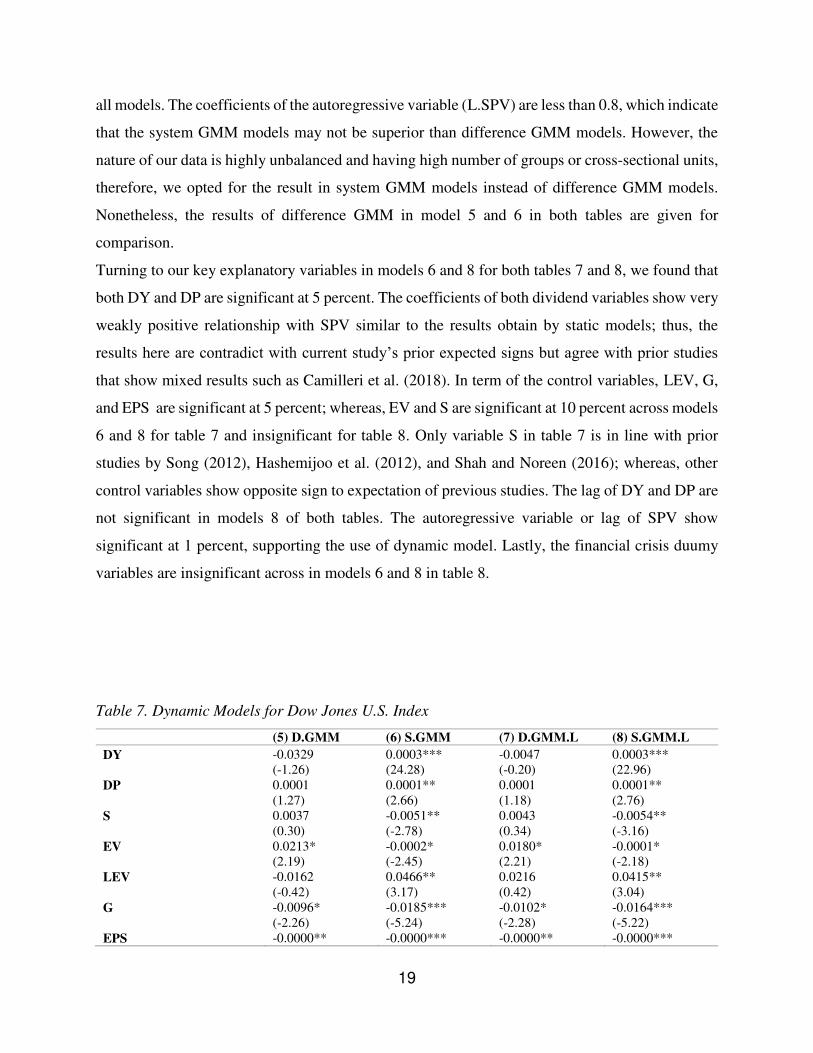
all models. The coefficients of the autoregressive variable (L.SPV) are less than 0.8, which indicate

that the system GMM models may not be superior than difference GMM models. However, the

nature of our data is highly unbalanced and having high number of groups or cross-sectional units,

therefore, we opted for the result in system GMM models instead of difference GMM models.

Nonetheless, the results of difference GMM in model 5 and 6 in both tables are given for

comparison.

Turning to our key explanatory variables in models 6 and 8 for both tables 7 and 8, we found that

both DY and DP are significant at 5 percent. The coefficients of both dividend variables show very

weakly positive relationship with SPV similar to the results obtain by static models; thus, the

results here are contradict with current study’s prior expected signs but agree with prior studies

that show mixed results such as Camilleri et al. (2018). In term of the control variables, LEV, G,

and EPS are significant at 5 percent; whereas, EV and S are significant at 10 percent across models

6 and 8 for table 7 and insignificant for table 8. Only variable S in table 7 is in line with prior

studies by Song (2012), Hashemijoo et al. (2012), and Shah and Noreen (2016); whereas, other

control variables show opposite sign to expectation of previous studies. The lag of DY and DP are

not significant in models 8 of both tables. The autoregressive variable or lag of SPV show

significant at 1 percent, supporting the use of dynamic model. Lastly, the financial crisis duumy

variables are insignificant across in models 6 and 8 in table 8.

Table 7. Dynamic Models for Dow Jones U.S. Index

(5) D.GMM (6) S.GMM (7) D.GMM.L (8) S.GMM.L DY -0.0329 0.0003*** -0.0047 0.0003***

(-1.26) (24.28) (-0.20) (22.96)

DP 0.0001 0.0001** 0.0001 0.0001**

(1.27) (2.66) (1.18) (2.76)

S 0.0037 -0.0051** 0.0043 -0.0054**

(0.30) (-2.78) (0.34) (-3.16)

EV 0.0213* -0.0002* 0.0180* -0.0001*

(2.19) (-2.45) (2.21) (-2.18)

LEV -0.0162 0.0466** 0.0216 0.0415**

(-0.42) (3.17) (0.42) (3.04)

G -0.0096* -0.0185*** -0.0102* -0.0164***

(-2.26) (-5.24) (-2.28) (-5.22)

EPS -0.0000** -0.0000*** -0.0000** -0.0000***

20

(-2.88) (-4.49) (-2.93) (-4.44)

L.DY

0.1019 0.0947

(1.61) (1.01)

L.DP

-0.0000 -0.0000

(-1.09) (-1.07)

L.SPV 0.5101*** 0.4224*** 0.5763*** 0.4842***

(5.53) (15.66) (5.56) (30.52)

_cons

0.4047***

0.3764***

(9.03)

(9.79) Prob > F 0 0 0 0

N 9638 11549 9468 11338

No. of Groups/cross-

section

1537 1788 1504 1760

No. of Instruments 12 13 14 13

Arellano-Bond AR (1) 0 0 0 0

Arellano-Bond AR (2) 0.603 0.699 0.223 0.227

Sargan Test of overid.

restrictions (p-value)

0.496 0.099 0.201 0.352

Hansen Test of overid.


0.223 0.188 0.252 0.126

Diff. Hansen tests of

exogeneity (p-value)

0.223 0.09 0.252 0.094


parentheses

Table 8. Dynamic Models for Dow Jones U.S. Index with Crisis Dummy

(5) D.GMM (6) S.GMM (7) D.GMM.L (8) S.GMM.L DY -0.0442 0.0004*** -0.0191 0.0004***

(-1.39) (6.40) (-1.07) (6.86)

DP 0.0001 0.0001** 0.0001 0.0001**

(1.18) (3.13) (1.80) (3.08)

S -0.0008 -0.0023 0.0015 -0.0029

(-0.08) (-0.97) (0.13) (-1.40)

EV 0.0195*** -0.0000 0.0209*** -0.0000

(3.55) (-0.27) (3.77) (-0.41)

LEV -0.0257 0.0374** 0.0016 0.0388**

(-0.82) (2.75) (0.05) (2.95)

G -0.0116** -0.0157*** -0.0109** -0.0150***

(-3.12) (-4.13) (-2.58) (-4.40)

EPS -0.0000** -0.0000*** -0.0000** -0.0000***

(-2.90) (-4.14) (-2.85) (-4.53)

21

FCD -0.0816*** 0.1384 -0.0671** 0.1423

(-4.37) (1.69) (-2.92) (1.88)

L.DY

0.1030 0.0653

(1.44) (0.80)

L.DP

-0.0000 -0.0000

(-0.67) (-0.12)

L.SPV 0.3494*** 0.5284*** 0.4675*** 0.5133***

(3.91) (7.89) (4.59) (23.69)

_cons

0.2721**

0.2930***

(3.11)

(5.03) Prob > F 0 0 0 0

N 9638 11549 9468 11338

No. of Groups 1537 1788 1504 1760


Arellano-Bond AR (1) 0 0 0 0

Arellano-Bond AR (2) 0.477 0.368 0.868 0.432



0.304 0.196 0.479 0.68



0.049 0.418 0.449 0.625



0.94 0.42 0.844 0.625


parentheses

We now turn to the regression based on the Islamic stocks in Dow Jones U.S. Index. We also first

run static regression using POLS and Fixed effect estimators based on equation (1) and (2). The

results are shown in table 9 and table 10 (with the financial crisis dummy variable). We also found

that the models with the dummy in table 10 have considerably higher adjusted R-square but all

dummy variables are negatively significant opposite to that of the Dow Jones U.S. Index sample.

The model 3 in table 10 has the highest adjusted R-square of 0.0888. In contrast to the Dow Jones

U.S. Index, DY in Islamic stocks sample is not significant at 5 percent, but DP became

significant at 1 percent and shows negative relationship to SPV across all models with the

coefficient of less than 0.001. Despite weak coefficients, these results are consistent with

Hussainey et al. (2011) and Shah and Noreen (2016). Our control variables in table 10, S, EV, and

G are shown to be significant in POLS models (models 1 and 2) with all negative relationship.

Only variable S is in line with prior studies by Song (2012), Hashemijoo et al. (2012), and Shah

and Noreen (2016). The lag of DY is also shown to be positively significant. However, EV became

insignificant in the Fixed Effect models (model 3 and 4), but EPS become positively significant in

model 4 at 10 percent contradicting the prior studies.

Table 9. Static Models for Islamic Stocks in Dow Jones U.S. Index

(1) POLS (2) POLS.L (3) FixedE (4) FixedE.L

DY 0.8742*** 0.3498* 0.1658 -0.0323

22

(5.00) (2.23) (1.24) (-0.29)

DP -0.0001 -0.0001 -0.0002*** -0.0002***

(-0.62) (-1.01) (-3.88) (-3.31)

S -0.0106*** -0.0111*** -0.0624*** -0.0546***

(-5.46) (-5.77) (-7.77) (-6.96)

EV -0.0003*** -0.0003*** 0.0002 0.0002

(-3.67) (-3.69) (1.05) (0.94)

LEV 0.0083 0.0040 0.0090 -0.0050

(0.44) (0.21) (0.34) (-0.18)

G -0.0549*** -0.0545*** -0.0148* -0.0172**

(-6.83) (-6.43) (-2.29) (-2.85)

EPS -0.0005 -0.0004 0.0002* 0.0002**

(-1.08) (-1.09) (2.14) (3.16)

L.DY

1.0771***

0.5623**

(5.12)

(3.17)

L.DP

-0.0000

-0.0001

(-0.11)

(-0.86)

_cons 0.7174*** 0.7179*** 1.8675*** 1.6908***

(17.02) (17.04) (10.57) (9.78) Prob > F 0 0 0 0

Adjusted 𝑹𝟐 0.0371 0.0518 0.053 0.0502

N 4834 4479 4834 4479

No. of Groups

561 547


parentheses, correlated random effects - Hausman test showed p-value of 0, we reject the null hypothesis that


Table 10. Static Models for Islamic Stocks in Dow Jones U.S. Index with Crisis Dummy

(1) POLS (2) POLS.L (3) FixedE (4) FixedE.L

DY 0.9307*** 0.4044* 0.2789* 0.0786

(5.26) (2.51) (2.25) (0.77)

DP -0.0001 -0.0002 -0.0002*** -0.0002***

(-0.99) (-1.41) (-3.59) (-3.34)

S -0.0112*** -0.0117*** -0.0732*** -0.0695***

(-5.76) (-6.09) (-8.91) (-8.51)

EV -0.0004*** -0.0003*** 0.0002 0.0001

(-3.87) (-3.90) (0.95) (0.78)

LEV 0.0063 0.0017 0.0081 -0.0044

(0.34) (0.09) (0.30) (-0.16)

G -0.0556*** -0.0550*** -0.0132* -0.0146*

(-6.78) (-6.36) (-2.13) (-2.51)

EPS -0.0005 -0.0004 0.0002 0.0002*

(-1.07) (-1.09) (1.75) (2.49)

FCD -0.0421*** -0.0384*** -0.0634*** -0.0621***

23

(-6.33) (-5.74) (-13.70) (-13.03)

L.DY

1.0816***

0.5868***

(5.26)

(3.98)

L.DP

-0.0000

-0.0001

(-0.36)

(-1.60)

_cons 0.7358*** 0.7359*** 2.1147*** 2.0275***

(17.43) (17.49) (11.69) (11.26)

Prob > F 0 0 0 0

Adjusted 𝑹𝟐 0.0438 0.0577 0.0888 0.0874

N 4834 4479 4834 4479

No. of Groups

561.0000 547.0000


parentheses, correlated random effects - Hausman test showed p-value of 0, we reject the null hypothesis that Random

effect model is appropriate.

Regardless of the results in tables 9 and 10, the result obtained through dynamic GMM models in

tables 11 and 12 should provide more consistent and efficient explanations due to the limitation of

static models. As in the case of the Dow Jones U.S. Index, we still treat all variables as exogeneous

with the exception of EV and limit the instruments of the explanatory variables, to minimize the

overidentification problem. The diagnostic statistics in tables 11 and 12 for all models show that

there is no problem of autocorrelation of order 2 and overidentification. Moreover, the

specification of instrument used are validated based on the difference-in-Hansen test statistics,

showing the p-values of more than 5 percent. Similarly, we opted for the result system GMM

models rather than difference GMM models due to the nature of our data, despite the

autoregressive coefficients of less than 0.8 in most models.

Upon examining the dividend variables, we found that both DY and DP are not significant in all

models from both tables. In table 11, only control variable G in model 8 is significant at 5 percent.

In table 12 after controlling for the crisis period, the variable G are significant for models 6 and 8

at 5 percent and the variable lag of DY is significant at 5 percent. The crisis dummies also turn

out to be insignificant in all models. The autoregressive variable LSPV are only significant in

model 6 and 8 for both tables. The result here are in line with recent studies by Shah and Noreen

(2016) and Camilleri et al. (2018) initially, before dropping some control variables. However, the

result here could be affected by the present of outliners; therefore, robustness checks are made

using quantile regressions, which show the effect of the explanatory variables at different quantile

of SPV.

Table 11. Dynamic Models for Islamic Stocks in Dow Jones U.S. Index

(5) D.GMM (6) S.GMM (7) D.GMM.L (8) S.GMM.L DY 0.6953 0.1521 -0.6623 -2.0637

24

(0.40) (0.11) (-0.23) (-1.45)

DP 0.0382 -0.0016 0.0674 0.0262

(1.59) (-0.17) (1.10) (1.41)

S 0.0086 -0.0003 -0.0433 -0.0000

(0.17) (-0.06) (-0.92) (-0.01)

EV 0.0191 0.0086 0.0126 0.0055

(1.81) (1.43) (1.21) (1.74)

LEV 0.0080 -0.0030 0.0272 0.0258

(0.07) (-0.12) (0.10) (0.43)

G -0.0075 -0.0126 0.0010 -0.0205**

(-0.49) (-1.27) (0.07) (-2.62)

EPS -0.0001 -0.0003 -0.0000 -0.0002

(-0.54) (-0.80) (-0.09) (-0.86)

L.DY

0.2782 1.0111

(0.17) (1.42)

L.DP

-0.0011 -0.0002

(-0.46) (-0.70)

L.SPV 0.9272 0.6822*** 0.3827 0.6126***

(1.96) (4.38) (0.73) (4.35)

_cons

0.1493*

0.1806

(1.98)

(1.60) Prob > F 0.006 0 0.001 0

N 3949 4542 3895 4479

No. of Groups 511 553 509 547


Arellano-Bond AR (1) 0.207 0.939 0.092 0.207

Arellano-Bond AR (2) 0.729 0.178 0.285 0.827



0.992 0.42 0.977 0.957



0.52 0.11 0.813 0.43



0.52 0.26 0.813 0.303


parentheses

Table 12. Dynamic Models for Islamic Stocks in Dow Jones U.S. Index with Crisis Dummy

(5) D.GMM (6) S.GMM (7) D.GMM.L (8) S.GMM.L

DY -1.9651 0.1734 -2.1550 0.1735

(-1.00) (0.99) (-0.76) (0.98)

DP 0.0375 -0.0000 0.0423 -0.0001

(1.27) (-0.70) (1.92) (-0.69)

S -0.0486 -0.0026 -0.0859* -0.0052

(-0.73) (-1.03) (-2.34) (-1.72)

EV 0.0125 0.0000 0.0018 -0.0001

(1.08) (0.08) (0.19) (-0.80)

LEV 0.1247 0.0060 0.2288 0.0061

(1.78) (0.40) (1.44) (0.36)

G -0.0057 -0.0177** 0.0096 -0.0192**

(-0.22) (-3.09) (0.49) (-3.28)

EPS -0.0001 -0.0001 0.0000 -0.0001

(-0.56) (-0.91) (0.90) (-0.90)

FCD 0.0106 0.0881 0.0049 0.0543

(0.31) (1.78) (0.21) (0.70)

L.DY

0.8986 0.5306**

25

(0.80) (2.68)

L.DP

-0.0010 0.0001

(-0.58) (0.64)

L.SPV 0.2904 0.5310*** 0.0580 0.4451***

(0.61) (9.10) (0.17) (13.83)

_cons

0.2655***

0.3643***

(3.35)

(4.47)

Prob > F 0 0 0 0

N 3949 4542 3895 4479

No. of Groups 511 553 509 547.


Arellano-Bond AR (1) 0.354 0 0.094 0

Arellano-Bond AR (2) 0.516 0.093 0.313 0.212



0.999 0.62 0.942 0.547


Restrictions (p-value)

0.231 0.583 0.572 0.439



0.589 0.815 0.271 0.439


parentheses

Robustness Analysis

As prior studies such as Camilleri et al. (2018) noted, dividend policy variables may show tendency

to be fluid and can be sensitive to the treatment of outliers and sampling procedures. For instant

DY or DP may become more significant explanatory than each other or change in directions of

relationship of DY and DP to SPV. Consequently, additional regressions are tested to address

these issues using simultaneous quantile regressions based on equation (3). The simultaneous

quantile regressions show the effect of the explanatory variables at different quantiles of SPV;

hence, they give better estimations when there are outliners, which is expected within our sample

due to large number of firms. Moreover, the estimations given at different quantiles can also

represent classes of stocks such as low SPV stock may refer to more mature, “leaders” , or “value”

stocks, while high SPV stocks may refer to more speculative stocks.

Tables 13 and 14 present the results of quantile estimations at 10, 25, 50, 75, and 90 percent

quantiles for the Dow Jones U.S. Index stocks without and with crisis dummy respectively. Figures

1 and 2 (appendix) show the effects of each variables for all quantiles within (0, 1) range of SPV.

In both tables, we found that both dividend variables are not significant at any percentage points

of quantiles. The results here prove the sensitivity to outliners of the study and also show that the

weak coefficients (less than 0.001) obtained from system GMM cannot affect the SPV after we

control for outliners. Thus, quintile regression strengthens the our suspicious of weak coefficients

of the dividend variables. The results for control variables show little difference across quantile

26

except for EPS, which is significant at 75 and 90 percent quantile in both tables. The financial

crisis dummy variable become significant similar to those in static models.

Table 13. Quantile Regressions for the Dow Jones U.S. Index

q10 q25 q50 q75 q90

DY 0.00061 0.00050 0.00036 0.00017 -0.00007

[0.05] [0.07] [0.19] [0.37] [0.46]

DP 0.00013 0.00010 0.00005 0.00074 0.00367

[0.00] [0.00] [0.00] [0.00] [0.00]

S -0.01057*** -0.01262*** -0.01123*** -0.00859*** -0.01472***

[0.00] [0.00] [0.00] [0.00] [0.00]

EV 0.00008 -0.00002 -0.00022 -0.00062 -0.00080*

[0.00] [0.00] [0.00] [0.00] [0.00]

LEV 0.05802*** 0.04402*** 0.04721*** 0.07755*** 0.13660***

[0.01] [0.01] [0.01] [0.02] [0.03]

G -0.07395*** -0.06618*** -0.06275*** -0.05004*** -0.04822*

[0.01] [0.01] [0.01] [0.01] [0.02]

EPS 0.00000 -0.00000 -0.00001 -0.00002*** -0.00003***

[0.00] [0.00] [0.00] [0.00] [0.00]

_cons 0.54597*** 0.67253*** 0.74183*** 0.80643*** 1.08546***

[0.03] [0.03] [0.03] [0.05] [0.07]


brackets, Robustness using bootstrap replications of 1000 standard error

Table 14. Quantile Regressions for the Dow Jones U.S. Index with Crisis Dummy

q10 q25 q50 q75 q90

DY 0.00061 0.00049 0.00035 0.00016 -0.00009

[0.05] [0.09] [0.20] [0.39] [0.46]

DP 0.00013 0.00009 0.00004 0.00069 0.00362

[0.00] [0.00] [0.00] [0.00] [0.00]

S -0.01095*** -0.01326*** -0.01195*** -0.00981*** -0.01543***

[0.00] [0.00] [0.00] [0.00] [0.00]

EV 0.00004 -0.00003 -0.00024 -0.00065 -0.00083

[0.00] [0.00] [0.00] [0.00] [0.00]

LEV 0.05638*** 0.04812*** 0.04679*** 0.07112*** 0.12982***

[0.01] [0.01] [0.01] [0.02] [0.03]

G -0.07543*** -0.06650*** -0.06200*** -0.05055*** -0.04920**

[0.01] [0.01] [0.01] [0.01] [0.02]

EPS 0.00000 -0.00000 -0.00001 -0.00002*** -0.00003***

[0.00] [0.00] [0.00] [0.00] [0.00]

FCD -0.02628*** -0.03341*** -0.05185*** -0.08056*** -0.10993***

[0.01] [0.00] [0.01] [0.01] [0.01]

_cons 0.55851*** 0.68954*** 0.76296*** 0.84288*** 1.11068***

[0.03] [0.03] [0.03] [0.05] [0.07]

27



In the case of Islamic stocks in the Dow Jones U.S. Index, the results in tables 15 and 16 and

figures 3 and 4 (appendix) display that DY variables are significant at 5 percent across all quantiles

in contrast to the insignificant relationships found using system GMM models. Thus, a more

restrictive classes of stocks could provide significant relationship similar to prior studies’ sample

selection, which focus on smaller particular groups of stocks with consistent dividend payout. In

table 16, the coefficient of DY is higher in the upper quantile, and lowest in the 10 percent quantiles

at 0.87. Thus, DY has a direct affect SPV at around 1 to 1 ratio across all quantiles. Only control

variable G show significant relationship across all quantiles consistent with the result from system

GMM models. The financial crisis dummy proves to be significant here similar to the result in

static models.

Table 15. Quantile Regressions for Islamic Stocks in the Dow Jones U.S. Index

q10 q25 q50 q75 q90

DY 0.74828*** 0.89118*** 1.09417*** 1.02292** 1.18619**

[0.20] [0.20] [0.23] [0.35] [0.38]

DP 0.00020 0.00005 -0.00010 -0.00032 0.00055

[0.00] [0.00] [0.00] [0.00] [0.00]

S -0.00627 -0.00752 -0.00498 -0.00440 -0.00875*

[0.00] [0.00] [0.00] [0.00] [0.00]

EV 0.00021 0.00003 -0.00013 -0.00040 -0.00083

[0.00] [0.00] [0.00] [0.00] [0.00]

LEV -0.00617 -0.01032 -0.02945 -0.00752 0.02932

[0.02] [0.02] [0.02] [0.02] [0.04]

G -0.06623*** -0.06349*** -0.05460*** -0.04878*** -0.04536**

[0.01] [0.01] [0.01] [0.01] [0.02]

EPS -0.00215 -0.00502 -0.00892 -0.01186** -0.01021***

[0.00] [0.00] [0.01] [0.00] [0.00]

_cons 0.44655*** 0.55284*** 0.59004*** 0.68742*** 0.90011***

[0.07] [0.08] [0.08] [0.09] [0.08]



28

Table 16. Quantile Regressions for Islamic Stocks in the Dow Jones U.S. Index with Crisis

Dummy

q10 q25 q50 q75 q90

DY 0.87259*** 0.93969*** 1.14751*** 1.23886*** 1.04923**

[0.23] [0.20] [0.27] [0.35] [0.39]

DP 0.00020 0.00004 -0.00014 -0.00036 0.00052

[0.00] [0.00] [0.00] [0.00] [0.00]

S -0.00612 -0.00854* -0.00552 -0.00577 -0.00962*

[0.00] [0.00] [0.00] [0.00] [0.00]

EV -0.00024 0.00001 -0.00027 -0.00043 -0.00084

[0.01] [0.00] [0.00] [0.00] [0.00]

LEV -0.02153 -0.01622 -0.01178 0.00315 0.04060

[0.02] [0.02] [0.02] [0.03] [0.04]

G -0.06725*** -0.06217*** -0.05459*** -0.05512*** -0.03770*

[0.01] [0.01] [0.01] [0.01] [0.01]

EPS -0.00225 -0.00511 -0.00922 -0.01157** -0.01091***

[0.00] [0.00] [0.01] [0.00] [0.00]

FCD -0.02059** -0.02157** -0.04227*** -0.06888*** -0.09242***

[0.01] [0.01] [0.01] [0.01] [0.02]

_cons 0.44949*** 0.58051*** 0.60605*** 0.72189*** 0.92692***

[0.07] [0.08] [0.09] [0.08] [0.09]

Note: *, **, ***Significant at 90, 95, and 99 percent level of confidence respectively, Standard

errors are in brackets, Robustness using bootstrap replications of 1000 standard error

Discussion

Majority of past studies suggest that dividend policy variables DY and DP are related to the SPV

based on different samples across the globe with mixed results in term of the directions of

relationship, while some of the studies show insignificant relationship. The inconclusive results

are mainly due to the variation in samples and technique deployed; however, prior studies

document the recurring problem of multicollinearity, unobserved heteroskedasticity, and outliners.

By using GMM methods and quantile regressions instead of static models, we are able to minimize

these problems. Our results offer new insight to the topic by using larger sample in both samples

of Islamic stocks and all stocks in the Dow Jones U.S. Index and by using the mentioned techniques

instead of reduction of variables. We are able retain the theoretical frameworks and their

implication of stock volatility.

Our results confirm that the financial crisis improves the explanatory power in the case of static,

difference GMM models, and quantile regressions, but not in the case of system GMM. Thus,

dividend policy may constitute minute effect on SPV than anticipated compare to other factor such

as trading setup, liquidity factors, macroeconomic factors, and international trade and finance,

which can be affected by the crisis (Camilleri et al. 2018).

29

Moreover, quantile regressions or sample clustering offers new insight about the dividend-SPV

relationship and strongly affected the coefficient of the DY and DP. The implication of the

changing in coefficients could due to the discrimination from investors in choosing the class of

stocks to invest, which can be describe in their volatilities. We also found that the dividend-SPV

relationship could react differently for a specific type of stocks such as Islamic stocks compare to

overall market. This phenomenon can be explained by the preferences of investors, the gaining

interest in ethical stocks, and the choice of portfolio diversification. Our results also show that past

dividend policies do not affect the present SPV negating the argument of longer horizon effect of

dividend policy.

Turning to the results of the Dow Jones U.S. index, we found that only DY is significant in system

GMM models with very weak coefficients and later turn out to be insignificant in quantile

regressions in both cases where we include and exclude financial crisis effect. Thus, at both overall

market level and each class of stocks, dividend contributes only a minor component to the SPV.

The results conform toward with the MM framework and EMH that dividend policy has become

less relevant. The implications of the finding are that investors are better inform about the

companies they invested as information are easily accessed and timely than before. Moreover, the

U.S. market present semi-strong to strong EMH, which also allow investors to formulate different

kinds of trading strategies over different horizons. We also found that larger size of a company

will have lower volatility, which due to the facts that larger companies are more diversified and

have stable earning. In addition, growing company and company that has higher EPS will have

less volatility. The contradicting results from prior studies here is due to the nature of companies

listed in the Dow Jones U.S. index, which is typically larger and more mature than companies in

developing market. It is not necessary that companies here are in growth stage and opted to retain

dividend, but the index has a mixed of technology companies, which also categorized by high

growth and has tendency to retain more cash. As Fama & French (2001) noted, there is a general

tendency for US-listed firms to become less likely to pay dividends in favor of pursuing growth-

oriented strategies which require extensive cash resources. Lastly, higher leverage contributes to

higher SPV, conforming the with theoretical explanation of stability of companies financing.

In the case of Islamic stocks in the Dow Jones U.S. Index, we did not find a significant relationship

between dividend and SPV at market level based on GMM models. The results here agree with

MM framework and EMH that dividend policy has become less relevant as that of the overall Dow

30

Jones U.S. Index. However, we found DY to be positively significant when examined according

to the class of stock based on the SPV. The results agree with the static models. The inferences

here could be that investors especially specific group of investors who concentrated on lower

leverage stocks or “value” stocks and ethical stocks are discriminating in choosing their own class

of stocks. Thus, changes in dividend yield such as dividend yield increase could serve as a

signaling tool for investors to buy more abruptly in that class of stocks that they are interested in

but may be indifferent in other classes of stocks. Hence, these investors could be specific “clients”

to each class of stock in the Dow Jones Islamic U.S. index or the lower leverage companies.

Moreover, DY affects more for higher volatility stocks compare to lower volatility stocks. The

implications here is that companies that has higher volatilities are relatively less mature and less

diversified or they could be the “laggard” companies compare to the companies with lower SPV

in the same industries. We also found that in both quantile regressions and GMM models, higher

asset growth will reduce the volatility. The companies classified in the Dow Jones Islamic U.S.

stocks have relative low leverage compare to overall market; hence, asset growth here can be proxy

for profitability, better management, and growth-oriented strategies instead of growing companies.

5. Conclusion

The relationship between dividend policy (DY and DP) and stock price volatility remains as a

“dividend puzzle” with supporting evidences for both dividend relevance and dividend irrelevance

theories. Examining this issue contributes to new insight and implication in corporate finance and

has direct implication for management adopting suitable dividend policy. It would help improve

investors’ judgment on their investment decision. Therefore, the purpose of our study is to shed

light on this puzzle by testing both conventional and Islamic equity with the use of relatively

advanced GMM methods and quantile regressive models. We investigate the relationship on stocks

in the Dow Jones U.S. Index controlling for size, asset growth, leverage ratio, EPS, and earning

volatility. We found that both GMM methods and quantile regressions provide deeper insight and

complement each other. The 2008-2009 crisis also constitutes better explanation of SPV. However,

past year’s dividend variables do not affect the present SPV.

We conclude that dividend policy contributes a minor component in the explanation of SPV. In

both cases of all stocks and Islamic stocks, dividend variables are not significant or has weak effect

on SPV as estimated by GMM models. Thus, the results follow the MM framework and EMH

indicating the less relevancy dividend overtime and a general tendency for US-listed firms such as

31

those in the technological sector to become less likely to pay dividends in pursuit of growth instead.

The results from quantile regression for all stocks also are in line with the GMM models; whereas,

the results from quantile regression for Islamic stocks show significant and strong positive

relationship between DY and SPV. This finding could indicate the dynamic of investors preference

and firms’ dividend policy. We found that investors who invested in Islamic stocks or low leverage

stock may have a discriminating tendency in choosing the class of stock according to their

preferences but may be indifferent to other classes of stocks. Thus, there could be clientele effect

in each class of stock for Islamic stocks.

Our study has three main contributions. First, our evidences contribute to the literature on dividend

policy. Second, our study helps both companies and investors to be better informed on stock price

reaction on dividend announcement. A recommendation for company can be made that it is less

relevant for dividend policy to affect stock prices especially increment or reduction in dividend

payout. Another recommendation for investor is that a higher dividend yield could excite the

investors as positive signal in Islamic or low leverage/ “value” stocks, to buy more of the same

class of stock they invested. Third, we contribute to the literature on the stability and potential

diversification of Islamic stocks. Overall, Islamic stocks in the Dow Jones U.S. Index are as stable

as non-Islamic stocks, but they also attract specific group of investors according to classes, which

relies on dividend yield as positive signal for the future.

The limitation of the study is the data is still highly unbalanced resulting in disagreement

between models as in the case of static and dynamic models, and the case of difference and

system GMM models. The future research can be extended by exploring new techniques such as

non-linear techniques and new proxy to better capture volatility.

32

References

Ajmi, A.N., Hammoudeh, S., Nguyen, D. K. & sarafrazi, S., 2014. How strong are the causal

relationships between Islamic stock markets and conventional financial systems? Evidence

from linear and nonlinear tests. Journal of International Financial Markets, Institutions and

Money, 28, 213–227.

Al-Khazali, O., Lean, H.H. & Samet, A., 2014. Do Islamic stock indexes outperform

conventional stock indexes? A stochastic dominance approach. Pacific-Basin Finance

Journal, 28, 29–46.

Allen, F., Bernardo, A.E. & Welch, I., 2000. A theory of dividends based on tax clienteles. The

Journal of Finance, 55(6), 2499–2536.

Arellano, M. & Bover, O., 1995. Another look at the instrumental variable estimation of error-

components models. Journal of econometrics, 68(1), 29–51.

Baskin, J., 1989. Dividend policy and the volatility of common stocks. The Journal of Portfolio

Management, 15(3), 19-25.

Black, F. & Scholes, M., 1974. The effects of dividend yield and dividend policy on common

stock prices and returns. Journal of financial economics, 1(1), 1–22.

Camilleri, S.J., Grima, L. and Grima, S., 2018. The effect of dividend policy on share price

volatility: An analysis of Mediterranean banks’ stocks. Managerial Finance, 45(2), 348-

364.

Dewandaru, G., Rizvi, A., Masih, R., Alhabshi, S.O. & Masih, M., 2014. Stock market co-

movements: Islamic versus conventional equity indices with multi-timescales analysis.

Economic Systems, 38(4), 553–571.

Fama, E.F. & French, K.R., 2001. Disappearing dividends: changing firm characteristics or

lower propensity to pay? Journal of Financial economics, 60(1), 3–43.

Hussainey, K., Oscar Mgbame, C. and Chijoke-Mgbame, A.M., 2011. Dividend policy and share

price volatility: UK evidence. The Journal of risk finance, 12(1), 57-68.

Miller, M.H. & Modigliani, F., 1961. Dividend policy, growth, and the valuation of shares. the

Journal of Business, 34(4), 411–433.

Roodman, D., 2009b. How to do xtabond2: An introduction to difference and system GMM in

Stata. The stata journal, 9(1), 86–136.

Saiti, B., Bacha, O.I. & Masih, M., 2016. Testing the conventional and Islamic financial market

contagion: evidence from wavelet analysis. Emerging Markets Finance and Trade, 52(8),

1832–1849.

Shah, S.A. and Noreen, U., 2016. Stock price volatility and role of dividend policy: Empirical

evidence from Pakistan. International Journal of Economics and Financial Issues, 6(2),

461-472.

Windmeijer, F., 2005. A finite sample correction for the variance of linear efficient two-step

GMM estimators. Journal of econometrics, 126(1), 25–51.

eﬀect of dividend policy on stock price volatility in the

Documents