ee123 digital signal processing - inst.eecs.berkeley.eduee123/sp18/notes/lecture3b.pdf–linear...
TRANSCRIPT
M. Lustig, EECS UC Berkeley
EE123Digital Signal Processing
Lecture 3BProperties of DFTFast Convolutions
some of the material was based on slides by J.M. Kahn
M. Lustig, EECS UC Berkeley
Announcements
• HW1 due today.
• Homework Slip policy (lowest grade homework will be dropped)
• Finish reading Ch. 8, start Ch. 9
• ham radio licensing lecture III Tonight 6:30-8pm Cory 521
M. Lustig, EECS UC Berkeley
Last Time
• Discrete Fourier Transform– Similar to DFS– Sampling of the DTFT (subtleties....more later)
– Properties of the DFT• Today
– Continue with properties –Linear convolution with DFT– Overlap-Add / Save method for fast convolutions
0
BBBBBBBBBB@
X[0]
.
.
.X[k]
.
.
.X[N � 1]
1
CCCCCCCCCCA
=
0
BBBBBBBBBBBBB@
W
00N
· · · W
0nN
· · · W
0(N�1)N
.
.
.
...
.
.
.
...
.
.
.
W
k0N
· · · W
kn
N
· · · W
k(N�1)N
.
.
.
...
.
.
.
...
.
.
.
W
(N�1)0N
· · · W
(N�1)nN
· · · W
(N�1)(N�1)N
1
CCCCCCCCCCCCCA
0
BBBBBBBBBB@
x[0]
.
.
.x[n]
.
.
.x[N � 1]
1
CCCCCCCCCCA
0
BBBBBBBBBB@
x[0]
.
.
.x[n]
.
.
.x[N � 1]
1
CCCCCCCCCCA
=1
N
0
BBBBBBBBBBBBB@
W
�00N
· · · W
�0kN
· · · W
�0(N�1)N
.
.
.
...
.
.
.
...
.
.
.
W
�n0N
· · · W
�nk
N
· · · W
�n(N�1)N
.
.
.
...
.
.
.
...
.
.
.
W
�(N�1)0N
· · · W
�(N�1)kN
· · · W
�(N�1)(N�1)N
1
CCCCCCCCCCCCCA
0
BBBBBBBBBB@
X[0]
.
.
.X[k]
.
.
.X[N � 1]
1
CCCCCCCCCCA
M. Lustig, EECS UC Berkeley
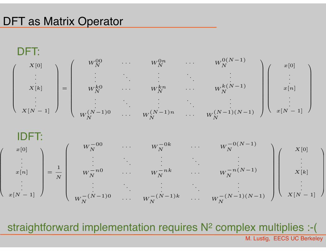
DFT as Matrix Operator
DFT:
IDFT:
straightforward implementation requires N2 complex multiplies :-(
M. Lustig, EECS UC Berkeley
DFT as Matrix Operator
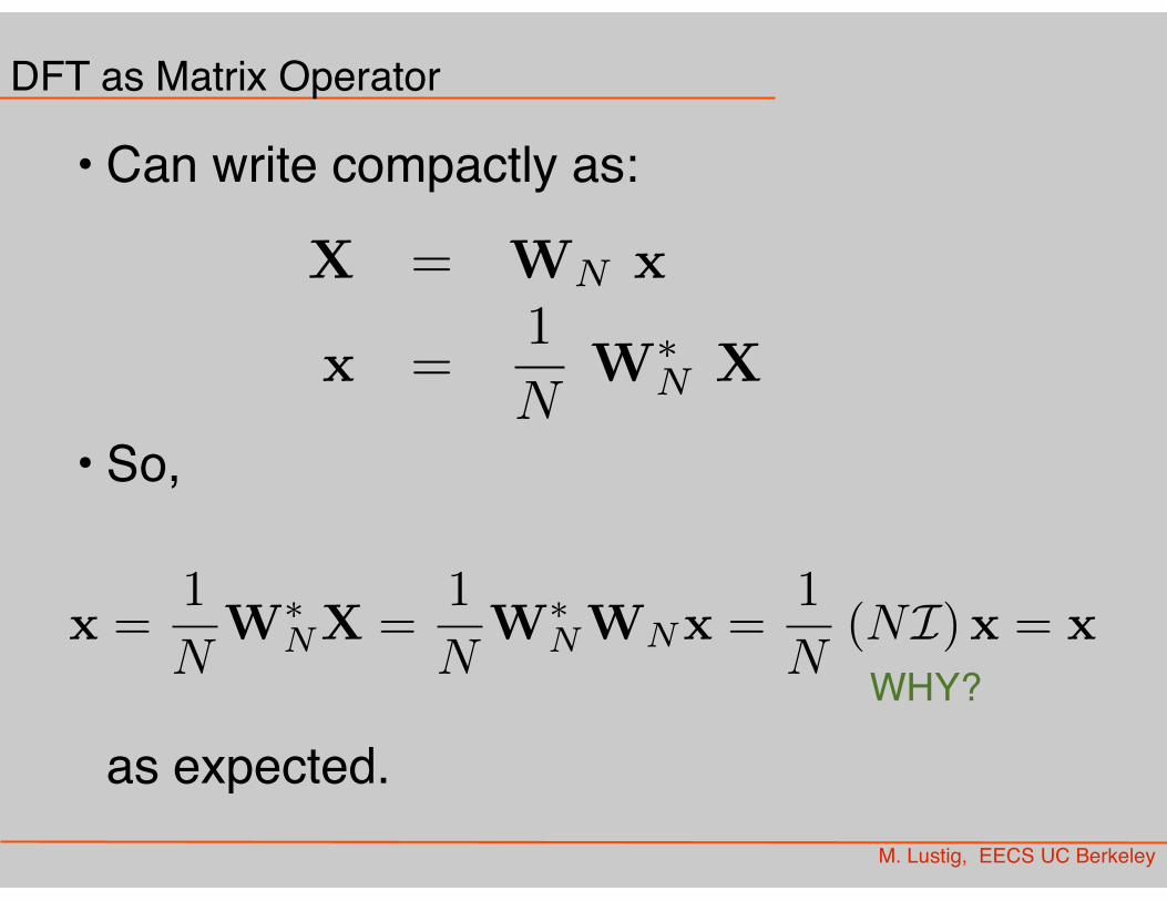
• Can write compactly as:
• So, as expected.
X = WN x
x =1
NW
⇤N X
x =1
NW
⇤NX =
1
NW
⇤NWNx =
1
N(NI)x = x
WHY?

x[((n�m))N ] $ X[k]e�j(2⇡/N)km = X[k]W kmN
M. Lustig, EECS UC Berkeley
Properties of DFT
• Inherited from DFS (EE120) so no need to be proved
• Linearity
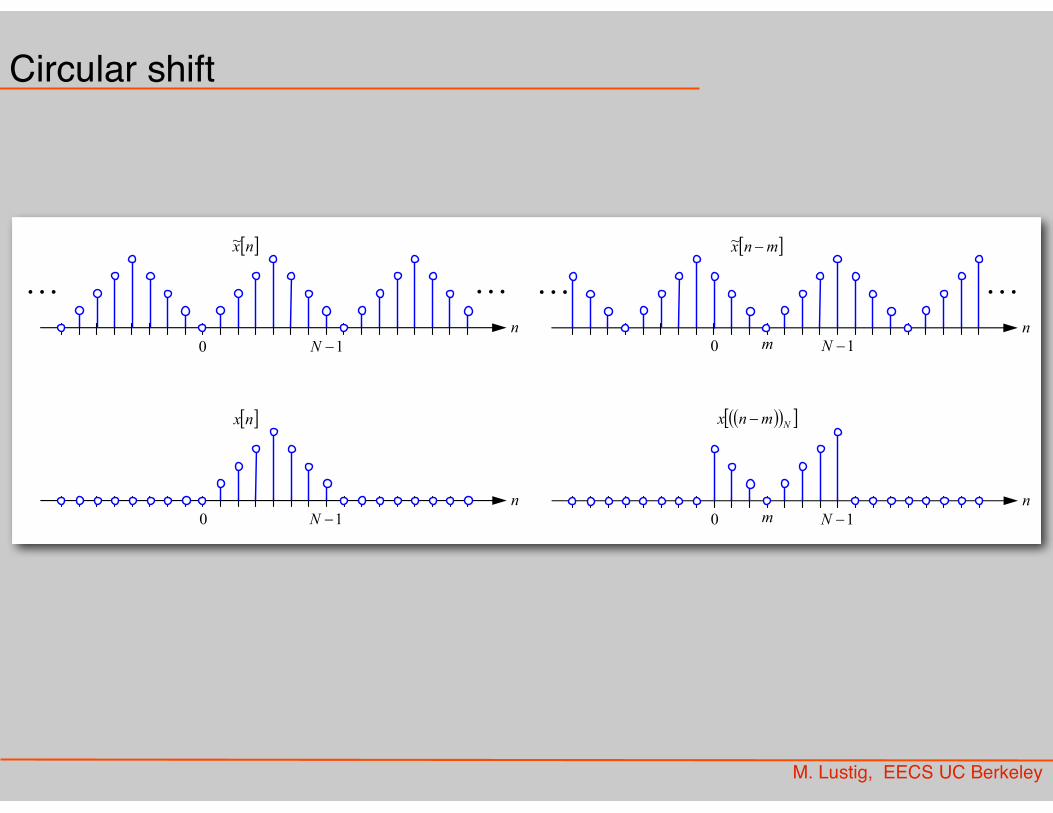
• Circular Sample Shift
↵1x1[n] + ↵2x2[n] $ ↵1X1[k] + ↵2X2[k]
M. Lustig, EECS UC Berkeley
Circular shift
! "mnx #~
n
0 1#N
. . . . . .
m
$ %$ %! "N
mnx #
n
0 1#Nm
! "nx~
n
0 1#N
. . . . . .
! "nx
n
0 1#N

M. Lustig, EECS UC Berkeley
Properties of DFT
• Circular frequency shift
• Complex Conjugation
• Conjugate Symmetry for Real Signals
x[n]ej(2⇡/N)nl = x[n]W�nlN $ X[((k � l))N ]
x
⇤[n] $ X
⇤[((�k))N ]
x[n] = x
⇤[n] $ X[k] = X
⇤[((�k))N ]
Show....

k
k
M. Lustig, EECS UC Berkeley
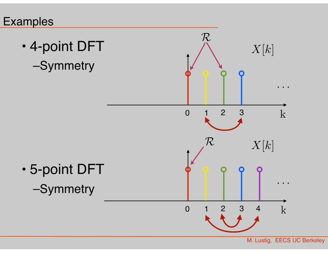
Examples
• 4-point DFT–Symmetry
• 5-point DFT–Symmetry
· · ·
0 1 2 3
X[k]
· · ·
0 1 2 3 4
X[k]
1 2 3
1 2 3 4
k
k
M. Lustig, EECS UC Berkeley
Examples
• 4-point DFT–Symmetry
• 5-point DFT–Symmetry
· · ·
0 1 2 3
X[k]
· · ·
0 1 2 3 4
X[k]
R
R
M. Lustig, EECS UC Berkeley
Properties of DFT
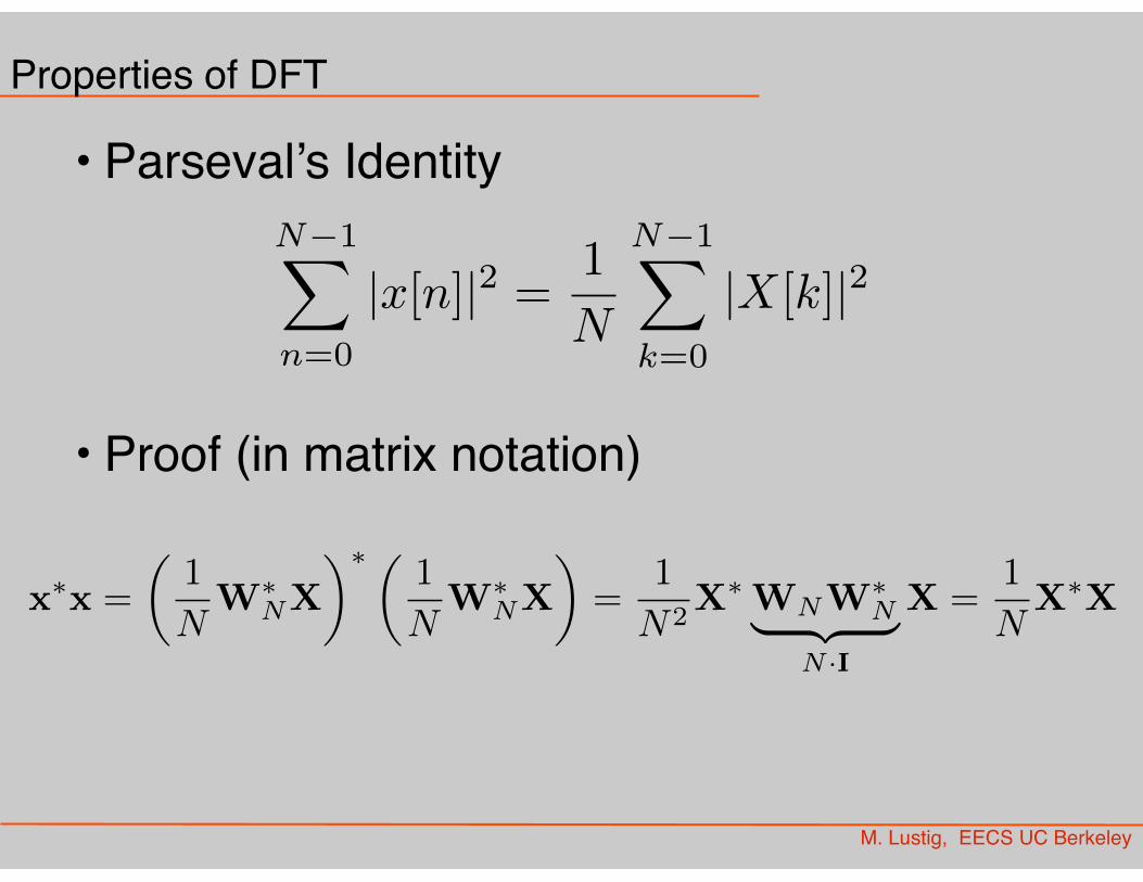
• Parseval’s Identity
• Proof (in matrix notation)
N�1X
n=0
|x[n]|2 =1
N
N�1X
k=0
|X[k]|2
x
⇤x =
✓1
NW
⇤NX
◆⇤ ✓ 1
NW
⇤NX
◆=
1
N2X
⇤WNW
⇤N| {z }
N ·I
X =1
NX
⇤X
M. Lustig, EECS UC Berkeley
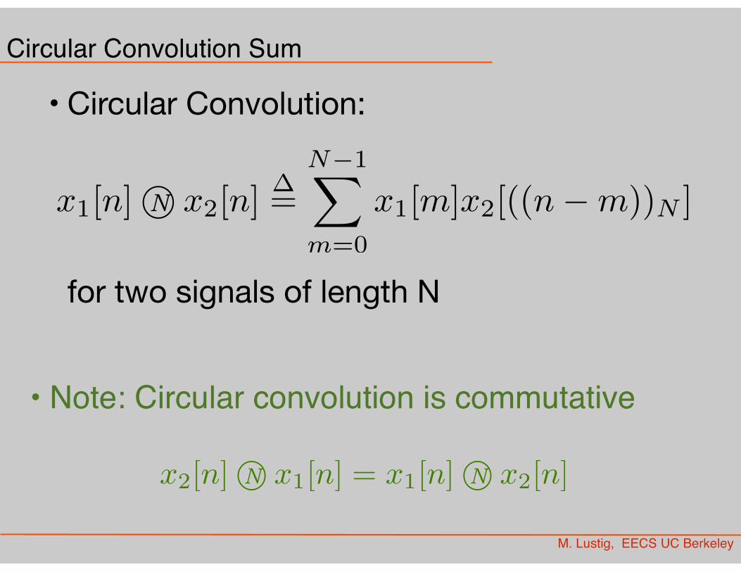
Circular Convolution Sum
• Circular Convolution:for two signals of length N
x1[n]�N x2[n]�=
N�1X
m=0
x1[m]x2[((n�m))N ]
x2[n]�N x1[n] = x1[n]�N x2[n]
• Note: Circular convolution is commutative
x1[n]
x2[n]
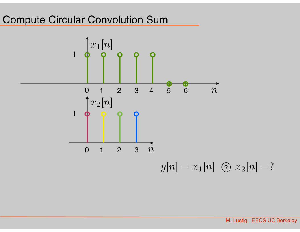
y[n] = x1[n] �7 x2[n] =?
M. Lustig, EECS UC Berkeley
Compute Circular Convolution Sum
n0 1 2 3 4
1
n0 1 2
1
5 6
3

x1[n]
x2[n]
M. Lustig, EECS UC Berkeley
Compute Circular Convolution Sum
n0 1 2 3 4
1
n0 1 2
1
5 6
3 4 5 6
Circular ‘flip’multiply and addHere: y[0]
y[n] = x1[n] �7 x2[n] =?
x1[n]
x2[n]
M. Lustig, EECS UC Berkeley
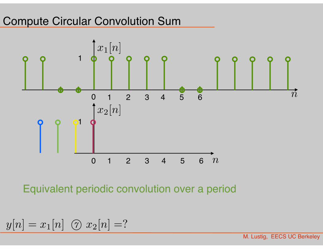
Compute Circular Convolution Sum
n0 1 2 3 4
1
n0 1 2
1
5 6
3 4 5 6
Equivalent periodic convolution over a period
y[n] = x1[n] �7 x2[n] =?
M. Lustig, EECS UC Berkeley
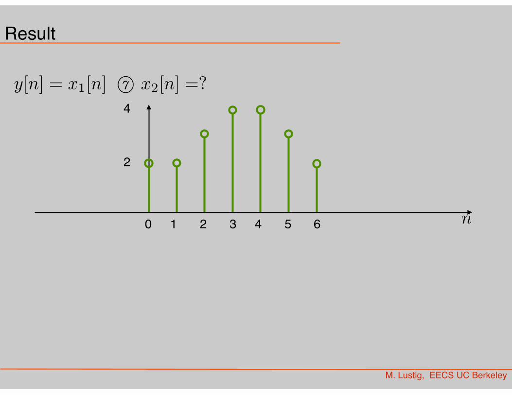
Result
n0 1 2 3 4
2
5 6
y[n] = x1[n] �7 x2[n] =?4
M. Lustig, EECS UC Berkeley
Properties of DFT
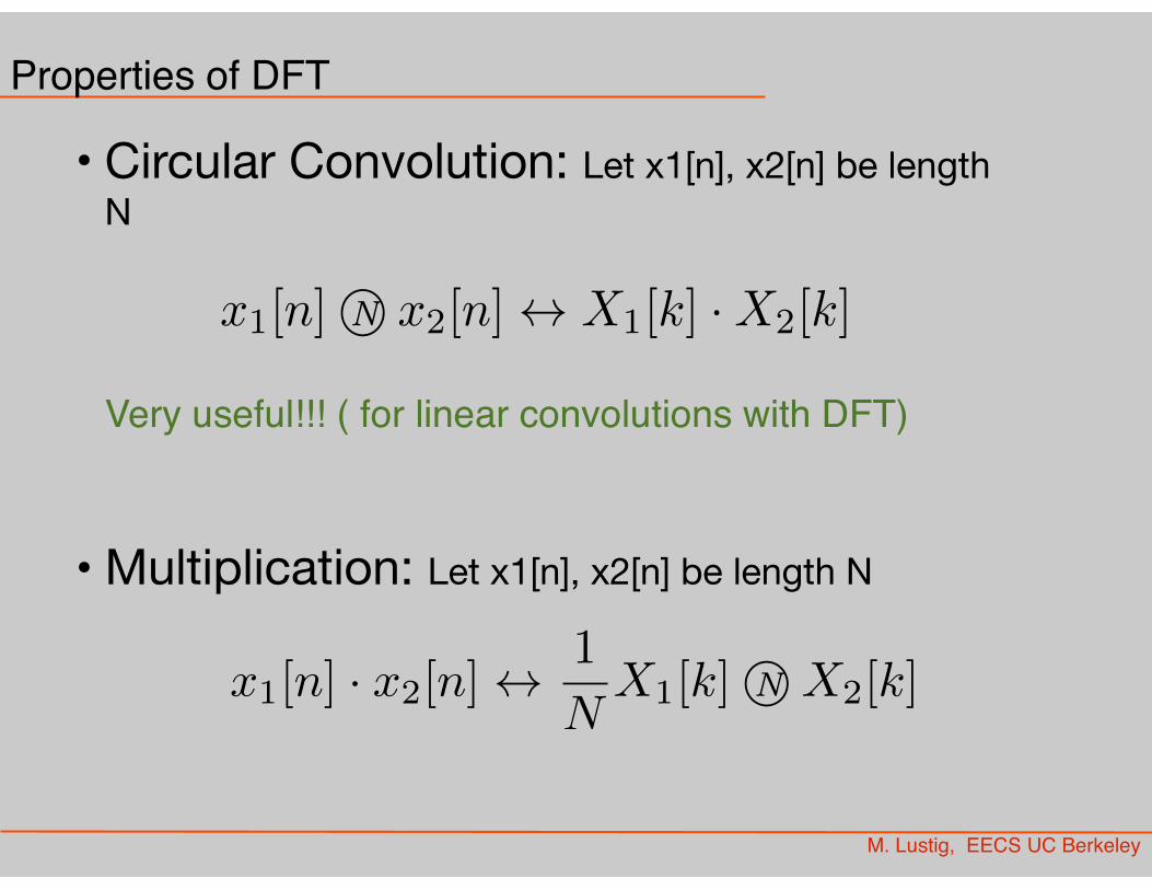
• Circular Convolution: Let x1[n], x2[n] be length N
• Multiplication: Let x1[n], x2[n] be length N
x1[n]�N x2[n] $ X1[k] ·X2[k]
x1[n] · x2[n] $1
N
X1[k]�N X2[k]
Very useful!!! ( for linear convolutions with DFT)
M. Lustig, EECS UC Berkeley
Linear Convolution
• Next....– Using DFT, circular convolution is easy – But, linear convolution is useful, not circular– So, show how to perform linear convolution with circular convolution
– Use DFT to do linear convolution

M. Lustig, EECS UC Berkeley
Linear Convolution
• We start with two non-periodic sequences:
• We want to compute the linear convolution:
• Requires L∙P multiplications
for example x[n] is a signal and h[n] an impulse response of a filter
x[n] 0 n L� 1
h[n] 0 n P � 1
y[n] = x[n] ⇤ h[n] =L�1X
m=0
x[m]h[n�m]
y[n] is nonzero for 0 ≤ n ≤ L+P-2 with length M=L+P-1
x1[n]
x2[n]
M. Lustig, EECS UC Berkeley
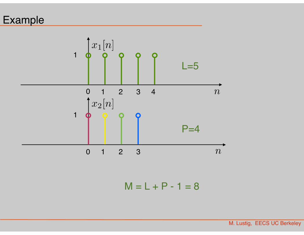
Example
n0 1 2 3 4
1
n0 1 2
1
3
L=5
P=4
M = L + P - 1 = 8
x1[n]
x2[n]
M. Lustig, EECS UC Berkeley
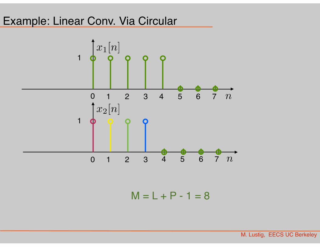
Example: Linear Conv. Via Circular
n0 1 2 3 4
1
n0 1 2
1
3
M = L + P - 1 = 8
6 75
4 6 75
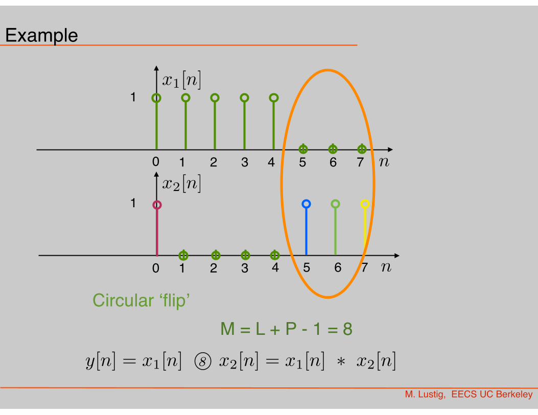
x1[n]
x2[n]
y[n] = x1[n] �8 x2[n] = x1[n] ⇤ x2[n]
M. Lustig, EECS UC Berkeley
Example
n0 1 2 3 4
1
n0 1 2
1
3
M = L + P - 1 = 8
6 75
4 6 75
Circular ‘flip’

M. Lustig, EECS UC Berkeley
Linear Convolution via Circular Convolution
• Zero-pad x[n] by P-1 zeros
• Zero-pad h[n] by L-1 zeros
• Now, both sequences are of length M=L+P-1
xzp[n] =
⇢x[n] 0 n L� 10 L n L+ P � 2
hzp[n] =
⇢h[n] 0 n P � 10 P n L+ P � 2
M. Lustig, EECS UC Berkeley
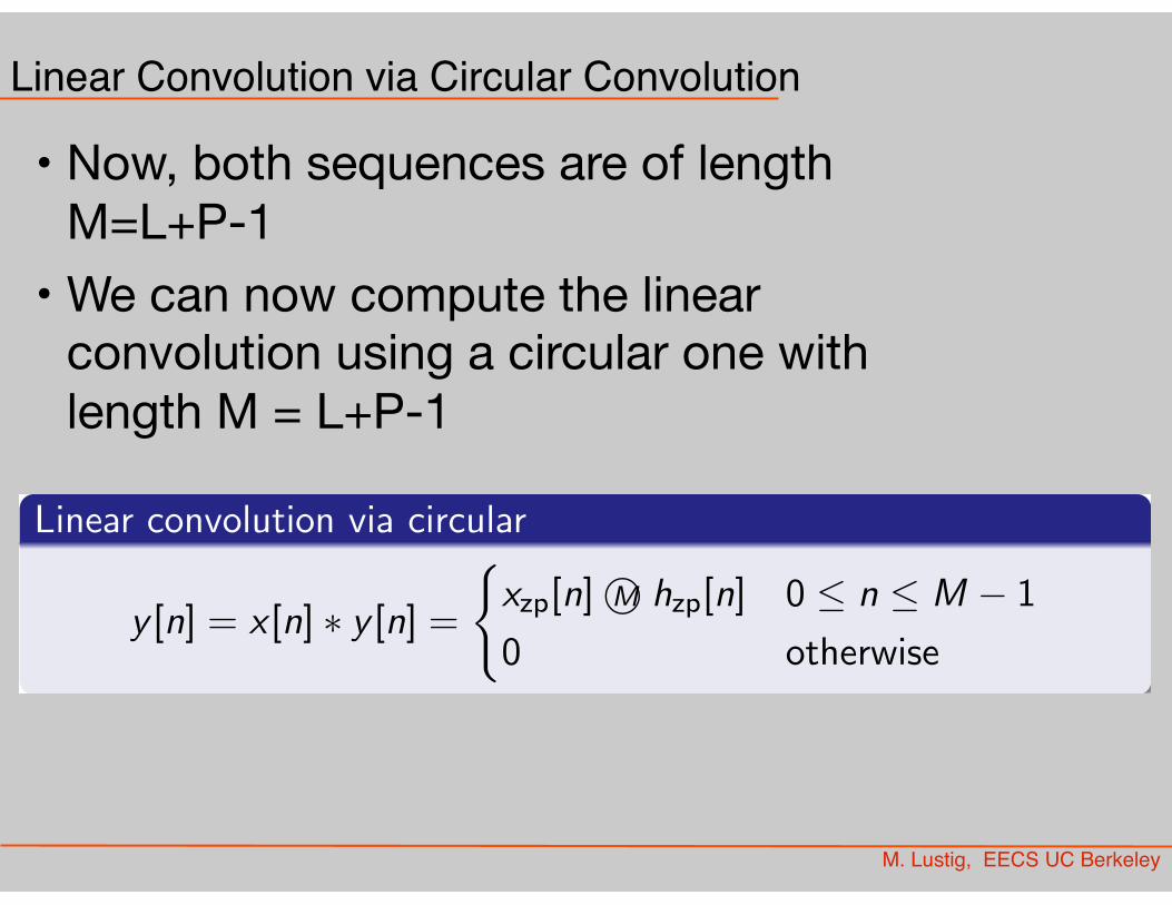
Linear Convolution via Circular Convolution
• Now, both sequences are of length M=L+P-1
• We can now compute the linear convolution using a circular one with length M = L+P-1
Linear Convolution using the DFT
Both zero-padded sequences xzp
[n] and hzp
[n] are of lengthM = L+ P � 1
We can compute the linear convolution x [n] ⇤ h[n] = y [n] bycomputing circular convolution x
zp
[n]�M hzp
[n]:
Linear convolution via circular
y [n] = x [n] ⇤ y [n] =(xzp
[n]�M hzp
[n] 0 n M � 1
0 otherwise
Miki Lustig UCB. Based on Course Notes by J.M Kahn Fall 2012, EE123 Digital Signal Processing

• In practice we can implement a circulant convolution using the DFT property:
M. Lustig, EECS UC Berkeley
Linear Convolution using DFT
x[n] ⇤ h[n] = xzp[n]�M hzp[n]
= DFT �1 {DFT {xzp[n]} · DFT {hzp[n]}}
for 0 ≤ n ≤ M-1, M=L+P-1
• Advantage: DFT can be computed with Nlog2N complexity (FFT algorithm later!)
• Drawback: Must wait for all the samples -- huge delay -- incompatible with real-time
M. Lustig, EECS UC Berkeley
Block Convolution
• Problem: – An input signal x[n], has very long length (could be considered infinite)
– An impulse response h[n] has length P– We want to take advantage of DFT/FFT and compute convolutions in blocks that are shorter than the signal
• Approach:– Break the signal into small blocks– Compute convolutions– Combine the results
M. Lustig, EECS UC Berkeley
Block Convolution
Example:
0 10 20 30
-0.5
0
0.5
n
x[n]
Input Signal, Length 33
0 10 20 30
-0.5
0
0.5
n
h[n]
Impulse Response, Length P = 6
0 10 20 30
-0.5
0
0.5
n
y[n]
Linear Convolution, Length 38
Miki Lustig UCB. Based on Course Notes by J.M Kahn Fall 2012, EE123 Digital Signal Processing
Block Convolution
Example:
0 10 20 30
-0.5
0
0.5
n
x[n]
Input Signal, Length 33
0 10 20 30
-0.5
0
0.5
n
h[n]
Impulse Response, Length P = 6
0 10 20 30
-0.5
0
0.5
n
y[n]
Linear Convolution, Length 38
Miki Lustig UCB. Based on Course Notes by J.M Kahn Fall 2012, EE123 Digital Signal Processing
Block Convolution
Example:
0 10 20 30
-0.5
0
0.5
n
x[n]
Input Signal, Length 33
0 10 20 30
-0.5
0
0.5
n
h[n]
Impulse Response, Length P = 6
0 10 20 30
-0.5
0
0.5
n
y[n]
Linear Convolution, Length 38
Miki Lustig UCB. Based on Course Notes by J.M Kahn Fall 2012, EE123 Digital Signal Processing
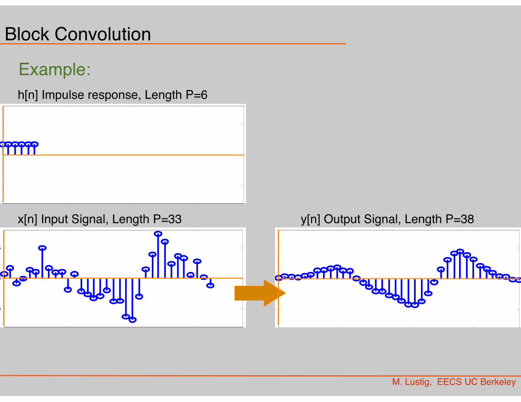
h[n] Impulse response, Length P=6
x[n] Input Signal, Length P=33 y[n] Output Signal, Length P=38
Block Convolution
Example:
M. Lustig, EECS UC Berkeley
Overlap-Add Method
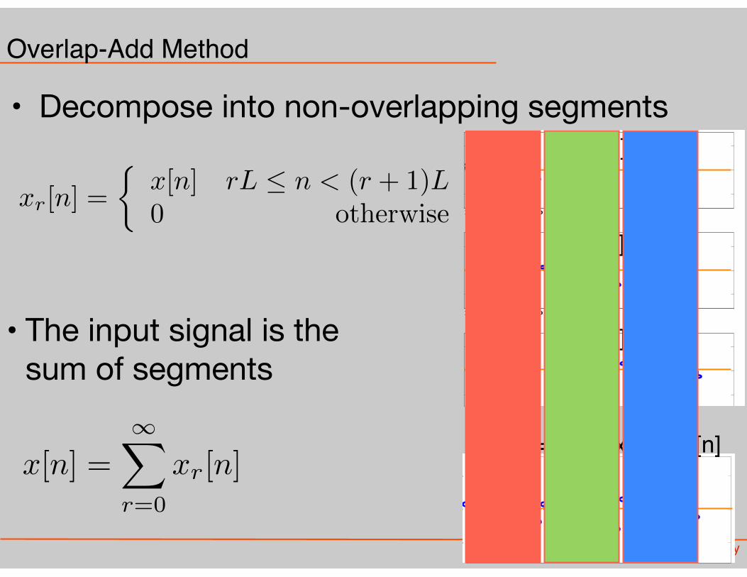
• Decompose into non-overlapping segmentsOverlap-Add Method
0 10 20 30
-0.5
0
0.5
n
x 0[n]
Overlap-Add, Input Segments, Length L = 11
0 10 20 30
-0.5
0
0.5
n
y 0[n]
Overlap-Add, Output Segments, Length L+P-1 = 16
0 10 20 30
-0.5
0
0.5
n
x 1[n]
0 10 20 30
-0.5
0
0.5
n
y 1[n]
0 10 20 30
-0.5
0
0.5
n
x 2[n]
0 10 20 30
-0.5
0
0.5
n
y 2[n]
0 10 20 30
-0.5
0
0.5
n
x[n]
Overlap-Add, Sum of Input Segments
0 10 20 30
-0.5
0
0.5
n
y[n]
Overlap-Add, Sum of Output Segments
Miki Lustig UCB. Based on Course Notes by J.M Kahn Fall 2012, EE123 Digital Signal Processing
Block Convolution
Example:
0 10 20 30
-0.5
0
0.5
n
x[n]
Input Signal, Length 33
0 10 20 30
-0.5
0
0.5
nh[n]
Impulse Response, Length P = 6
0 10 20 30
-0.5
0
0.5
n
y[n]
Linear Convolution, Length 38
Miki Lustig UCB. Based on Course Notes by J.M Kahn Fall 2012, EE123 Digital Signal Processing
x0[n]
x1[n]
x2[n]
x[n] = x0[n]+x1[n]+x2[n]
xr[n] =
⇢x[n] rL n < (r + 1)L
0 otherwise
• The input signal is the sum of segments
x[n] =1X
r=0
xr[n]
M. Lustig, EECS UC Berkeley
Overlap-Add Method
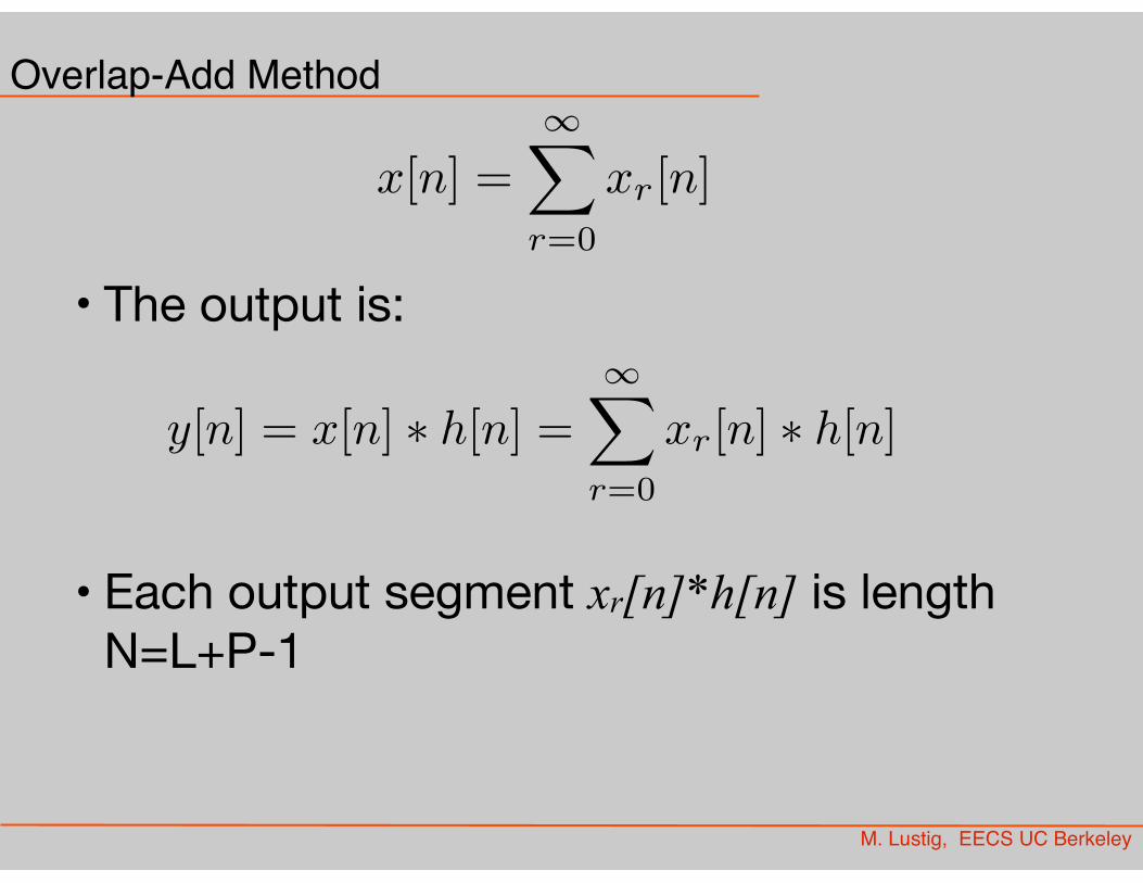
• The output is:
• Each output segment xr[n]*h[n] is length N=L+P-1
x[n] =1X
r=0
xr[n]
y[n] = x[n] ⇤ h[n] =1X
r=0
xr[n] ⇤ h[n]
M. Lustig, EECS UC Berkeley
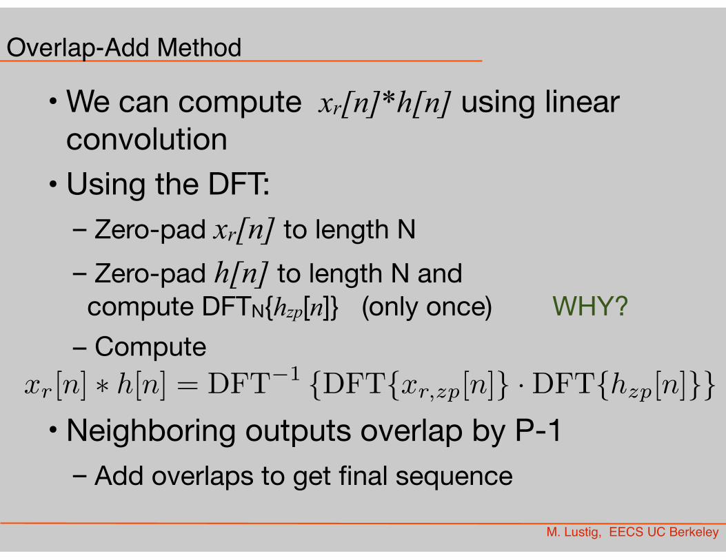
Overlap-Add Method
• We can compute xr[n]*h[n] using linear convolution
• Using the DFT:– Zero-pad xr[n] to length N– Zero-pad h[n] to length N and compute DFTN{hzp[n]} (only once) WHY?
– Compute
• Neighboring outputs overlap by P-1– Add overlaps to get final sequence
xr[n] ⇤ h[n] = DFT�1 {DFT{xr,zp[n]} ·DFT{hzp[n]}}
Overlap-Add Method
0 10 20 30
-0.5
0
0.5
n
x 0[n]
Overlap-Add, Input Segments, Length L = 11
0 10 20 30
-0.5
0
0.5
n
y 0[n]
Overlap-Add, Output Segments, Length L+P-1 = 16
0 10 20 30
-0.5
0
0.5
n
x 1[n]
0 10 20 30
-0.5
0
0.5
n
y 1[n]
0 10 20 30
-0.5
0
0.5
n
x 2[n]
0 10 20 30
-0.5
0
0.5
n
y 2[n]
0 10 20 30
-0.5
0
0.5
n
x[n]
Overlap-Add, Sum of Input Segments
0 10 20 30
-0.5
0
0.5
n
y[n]
Overlap-Add, Sum of Output Segments
Miki Lustig UCB. Based on Course Notes by J.M Kahn Fall 2012, EE123 Digital Signal Processing
Block Convolution
Example:
0 10 20 30
-0.5
0
0.5
n
x[n]
Input Signal, Length 33
0 10 20 30
-0.5
0
0.5
n
h[n]
Impulse Response, Length P = 6
0 10 20 30
-0.5
0
0.5
n
y[n]
Linear Convolution, Length 38
Miki Lustig UCB. Based on Course Notes by J.M Kahn Fall 2012, EE123 Digital Signal Processing
Block Convolution
Example:
0 10 20 30
-0.5
0
0.5
n
x[n]
Input Signal, Length 33
0 10 20 30
-0.5
0
0.5
n
h[n]
Impulse Response, Length P = 6
0 10 20 30
-0.5
0
0.5
n
y[n]
Linear Convolution, Length 38
Miki Lustig UCB. Based on Course Notes by J.M Kahn Fall 2012, EE123 Digital Signal Processing
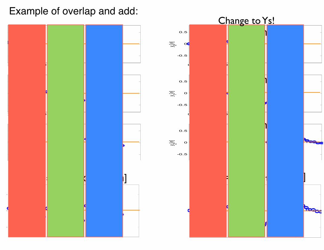
x0[n]
x1[n]
x2[n]
x[n] = x0[n]+x1[n]+x2[n] y[n] = y0[n]+y1[n]+y2[n]
x0[n]
x1[n]
x2[n]
Example of overlap and add:Change to Ys!

M. Lustig, EECS UC Berkeley
Overlap-Save Method
• Basic idea:• Split input into (P-1) overlapping segments
with length L+P-1
• Perform circular convolution in each segment, and keep the L sample portion which is a valid linear convolution
xr[n] =
⇢x[n] rL n < (r + 1)L+ P
0 otherwise
M. Lustig, EECS UC Berkeley
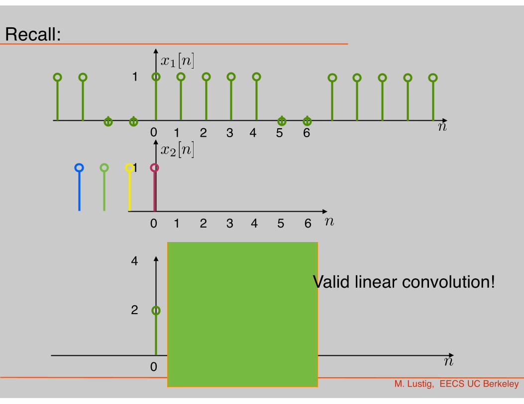
Recall:x1[n]
x2[n]
n0 1 2 3 4
1
n0 1 2
1
5 6
3 4 5 6
n0 1 2 3 4
2
5 6
4Valid linear convolution!

Overlap-Save Method
0 10 20 30
-0.5
0
0.5
n
y[n]
Overlap-Save, Concatenation of Usable Output Segments
0 10 20 30
-0.5
0
0.5
n
x 0[n]
Overlap-Save, Input Segments, Length L = 16
0 10 20 30
-0.5
0
0.5
n
y 0p[n
]
Overlap-Save, Output Segments, Usable Length L - P + 1
Usable (y0[n])
Unusable
0 10 20 30
-0.5
0
0.5
n
x 1[n]
0 10 20 30
-0.5
0
0.5
n
y 1p[n
]
Usable (y1[n])
Unusable
0 10 20 30
-0.5
0
0.5
n
x 2[n)
0 10 20 30
-0.5
0
0.5
n
y 2p[n
]
Usable (y2[n])
Unusable
Miki Lustig UCB. Based on Course Notes by J.M Kahn Fall 2012, EE123 Digital Signal Processing
Example of overlap and save: