M. Lustig, EECS UC Berkeley
EE123Digital Signal Processing
Lecture 3BProperties of DFTFast Convolutions
some of the material was based on slides by J.M. Kahn
M. Lustig, EECS UC Berkeley
Announcements
• HW1 due today.
• Homework Slip policy (lowest grade homework will be dropped)
• Finish reading Ch. 8, start Ch. 9
• ham radio licensing lecture III Tonight 6:30-8pm Cory 521
M. Lustig, EECS UC Berkeley
Last Time
• Discrete Fourier Transform– Similar to DFS– Sampling of the DTFT (subtleties....more later)
– Properties of the DFT• Today
– Continue with properties –Linear convolution with DFT– Overlap-Add / Save method for fast convolutions
0
BBBBBBBBBB@
X[0]
.
.
.X[k]
.
.
.X[N � 1]
1
CCCCCCCCCCA
=
0
BBBBBBBBBBBBB@
W
00N
· · · W
0nN
· · · W
0(N�1)N
.
.
.
...
.
.
.
...
.
.
.
W
k0N
· · · W
kn
N
· · · W
k(N�1)N
.
.
.
...
.
.
.
...
.
.
.
W
(N�1)0N
· · · W
(N�1)nN
· · · W
(N�1)(N�1)N
1
CCCCCCCCCCCCCA
0
BBBBBBBBBB@
x[0]
.
.
.x[n]
.
.
.x[N � 1]
1
CCCCCCCCCCA
0
BBBBBBBBBB@
x[0]
.
.
.x[n]
.
.
.x[N � 1]
1
CCCCCCCCCCA
=1
N
0
BBBBBBBBBBBBB@
W
�00N
· · · W
�0kN
· · · W
�0(N�1)N
.
.
.
...
.
.
.
...
.
.
.
W
�n0N
· · · W
�nk
N
· · · W
�n(N�1)N
.
.
.
...
.
.
.
...
.
.
.
W
�(N�1)0N
· · · W
�(N�1)kN
· · · W
�(N�1)(N�1)N
1
CCCCCCCCCCCCCA
0
BBBBBBBBBB@
X[0]
.
.
.X[k]
.
.
.X[N � 1]
1
CCCCCCCCCCA
M. Lustig, EECS UC Berkeley
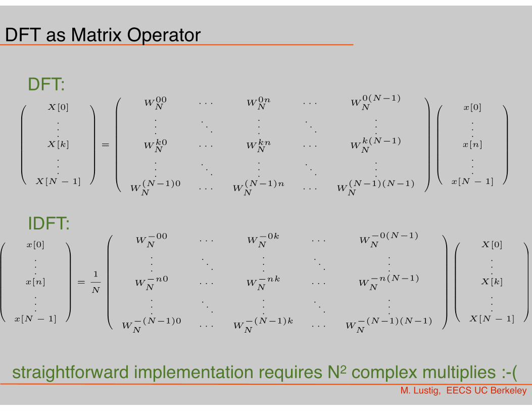
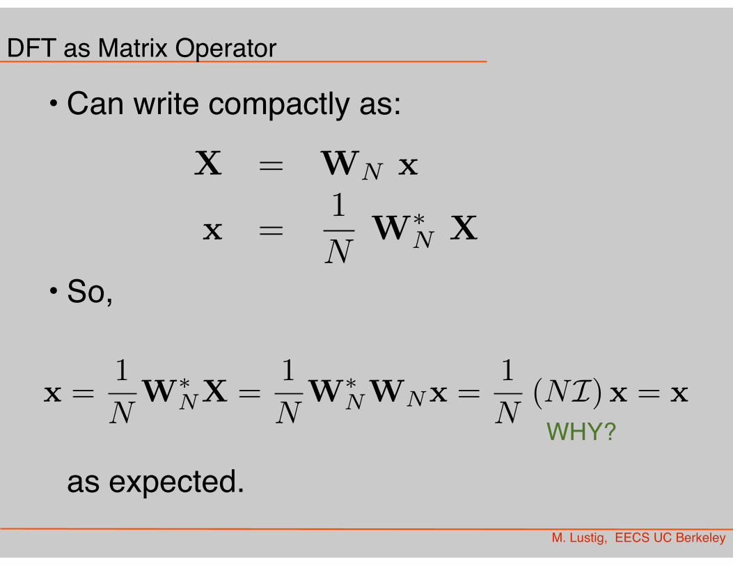
DFT as Matrix Operator
DFT:
IDFT:
straightforward implementation requires N2 complex multiplies :-(
M. Lustig, EECS UC Berkeley
DFT as Matrix Operator
• Can write compactly as:
• So, as expected.
X = WN x
x =1
NW
⇤N X
x =1
NW
⇤NX =
1
NW
⇤NWNx =
1
N(NI)x = x
WHY?

x[((n�m))N ] $ X[k]e�j(2⇡/N)km = X[k]W kmN
M. Lustig, EECS UC Berkeley
Properties of DFT
• Inherited from DFS (EE120) so no need to be proved
• Linearity
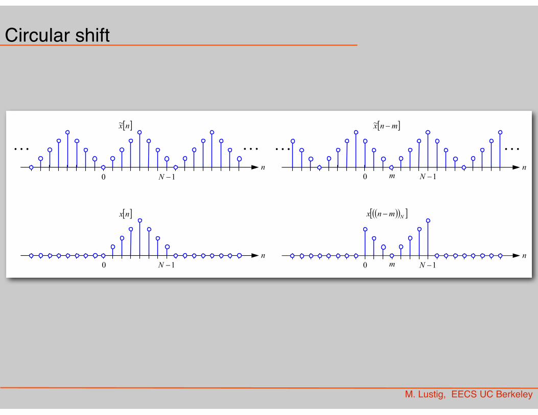
• Circular Sample Shift
↵1x1[n] + ↵2x2[n] $ ↵1X1[k] + ↵2X2[k]
M. Lustig, EECS UC Berkeley
Circular shift
! "mnx #~
n
0 1#N
. . . . . .
m
$ %$ %! "N
mnx #
n
0 1#Nm
! "nx~
n
0 1#N
. . . . . .
! "nx
n
0 1#N

M. Lustig, EECS UC Berkeley
Properties of DFT
• Circular frequency shift
• Complex Conjugation
• Conjugate Symmetry for Real Signals
x[n]ej(2⇡/N)nl = x[n]W�nlN $ X[((k � l))N ]
x
⇤[n] $ X
⇤[((�k))N ]
x[n] = x
⇤[n] $ X[k] = X
⇤[((�k))N ]
Show....

k
k
M. Lustig, EECS UC Berkeley
Examples
• 4-point DFT–Symmetry
• 5-point DFT–Symmetry
· · ·
0 1 2 3
X[k]
· · ·
0 1 2 3 4
X[k]
1 2 3
1 2 3 4
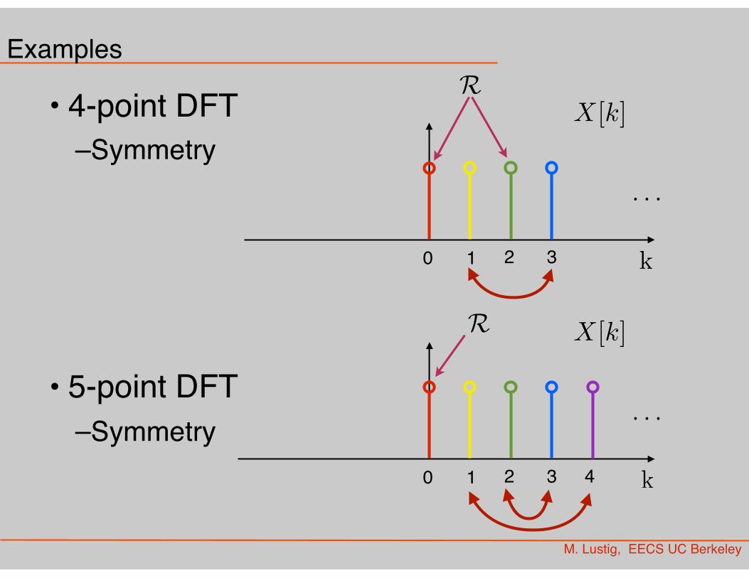
k
k
M. Lustig, EECS UC Berkeley
Examples
• 4-point DFT–Symmetry
• 5-point DFT–Symmetry
· · ·
0 1 2 3
X[k]
· · ·
0 1 2 3 4
X[k]
R
R
M. Lustig, EECS UC Berkeley
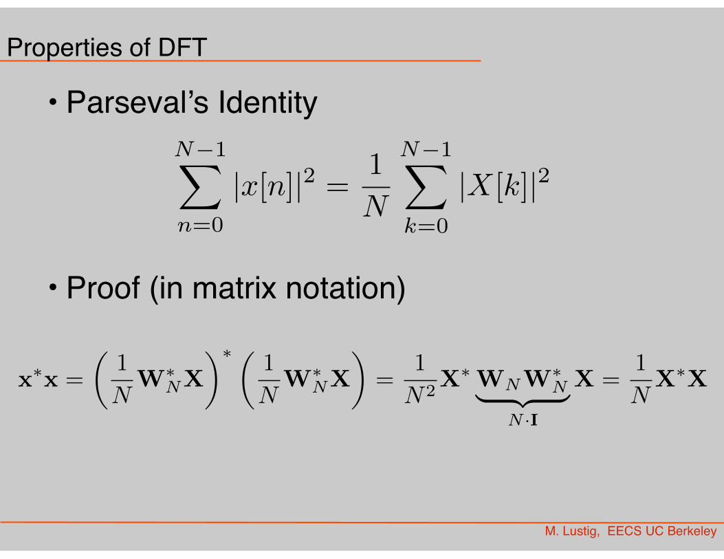
Properties of DFT
• Parseval’s Identity
• Proof (in matrix notation)
N�1X
n=0
|x[n]|2 =1
N
N�1X
k=0
|X[k]|2
x
⇤x =
✓1
NW
⇤NX
◆⇤ ✓ 1
NW
⇤NX
◆=
1
N2X
⇤WNW
⇤N| {z }
N ·I
X =1
NX
⇤X
M. Lustig, EECS UC Berkeley
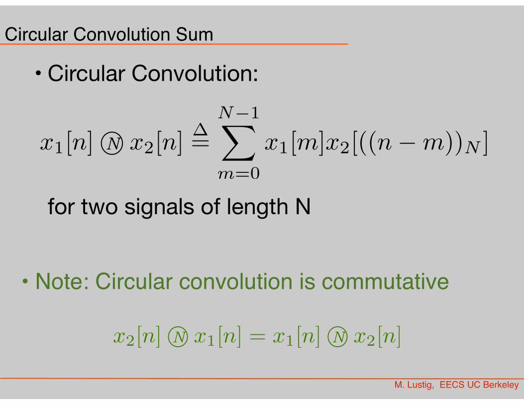
Circular Convolution Sum
• Circular Convolution:for two signals of length N
x1[n]�N x2[n]�=
N�1X
m=0
x1[m]x2[((n�m))N ]
x2[n]�N x1[n] = x1[n]�N x2[n]
• Note: Circular convolution is commutative
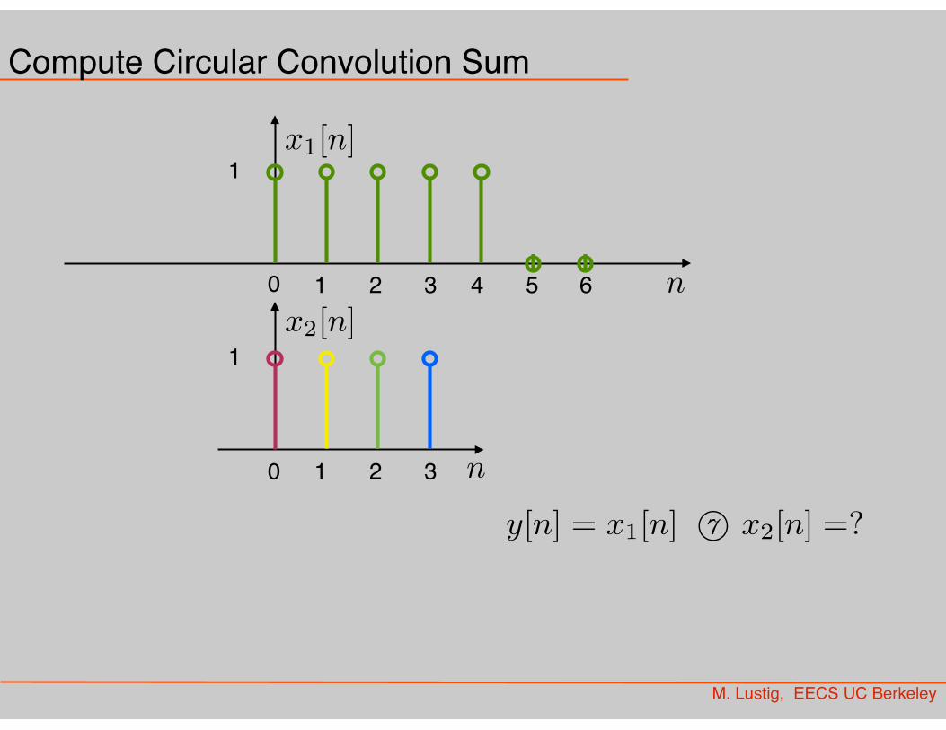
x1[n]
x2[n]
y[n] = x1[n] �7 x2[n] =?
M. Lustig, EECS UC Berkeley
Compute Circular Convolution Sum
n0 1 2 3 4
1
n0 1 2
1
5 6
3

x1[n]
x2[n]
M. Lustig, EECS UC Berkeley
Compute Circular Convolution Sum
n0 1 2 3 4
1
n0 1 2
1
5 6
3 4 5 6
Circular ‘flip’multiply and addHere: y[0]
y[n] = x1[n] �7 x2[n] =?
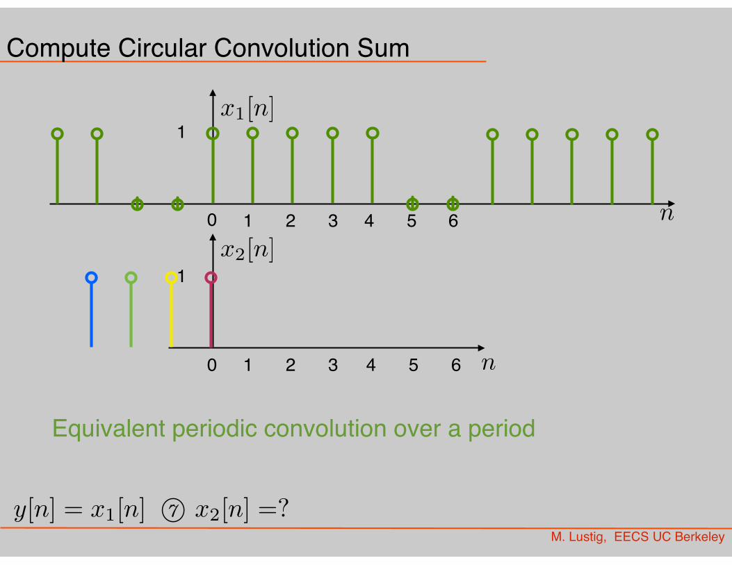
x1[n]
x2[n]
M. Lustig, EECS UC Berkeley
Compute Circular Convolution Sum
n0 1 2 3 4
1
n0 1 2
1
5 6
3 4 5 6
Equivalent periodic convolution over a period
y[n] = x1[n] �7 x2[n] =?
M. Lustig, EECS UC Berkeley
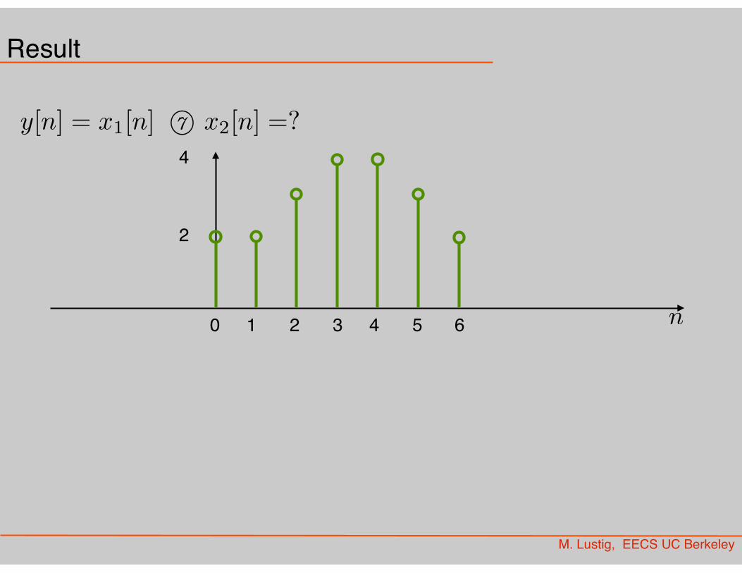
Result
n0 1 2 3 4
2
5 6
y[n] = x1[n] �7 x2[n] =?4
M. Lustig, EECS UC Berkeley
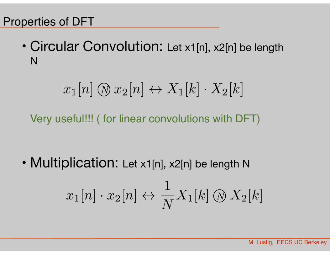
Properties of DFT
• Circular Convolution: Let x1[n], x2[n] be length N
• Multiplication: Let x1[n], x2[n] be length N
x1[n]�N x2[n] $ X1[k] ·X2[k]
x1[n] · x2[n] $1
N
X1[k]�N X2[k]
Very useful!!! ( for linear convolutions with DFT)
M. Lustig, EECS UC Berkeley
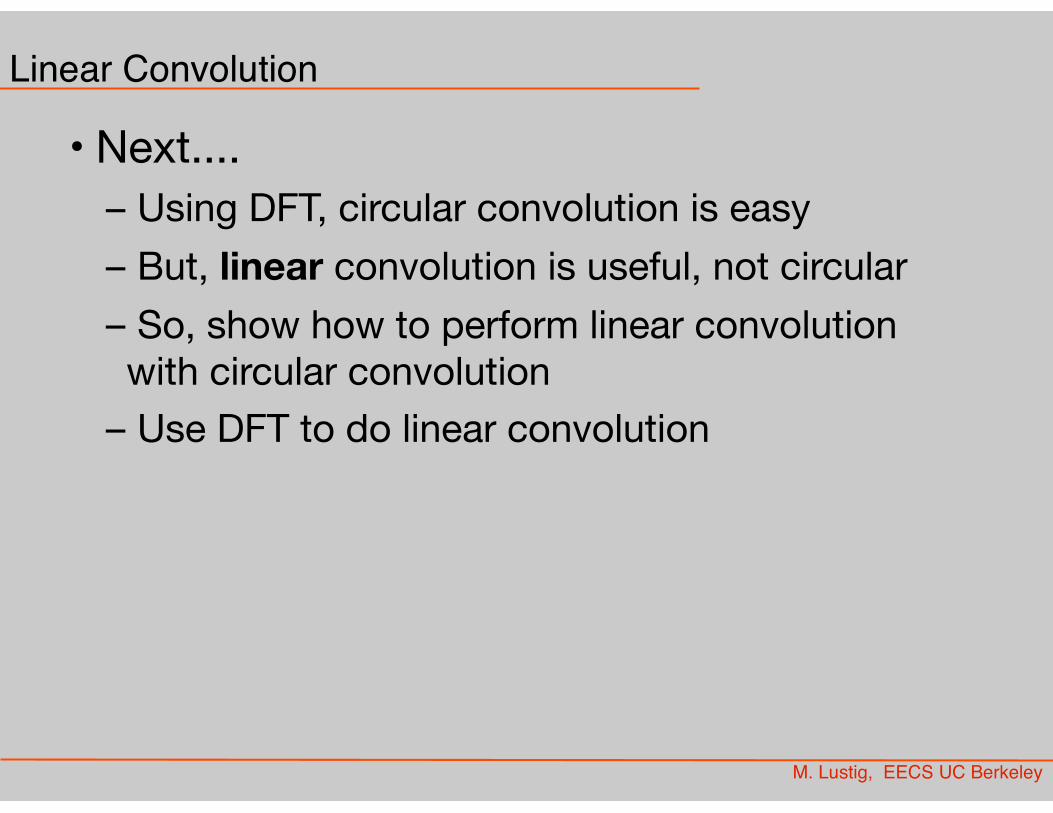
Linear Convolution
• Next....– Using DFT, circular convolution is easy – But, linear convolution is useful, not circular– So, show how to perform linear convolution with circular convolution
– Use DFT to do linear convolution

M. Lustig, EECS UC Berkeley
Linear Convolution
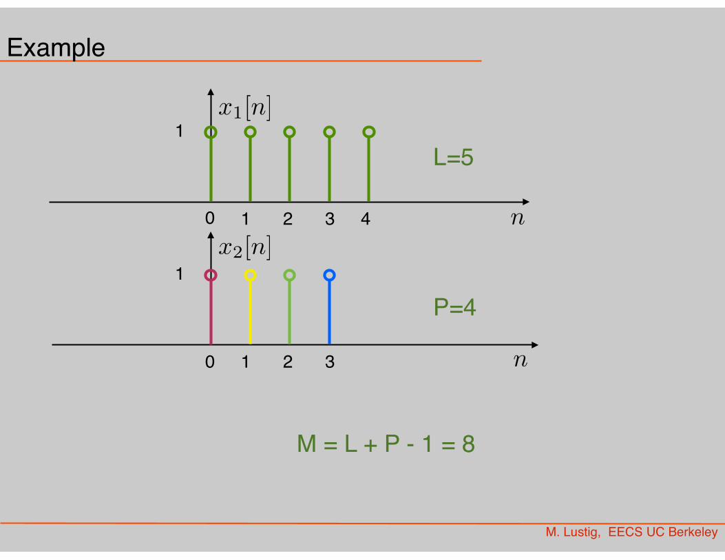
• We start with two non-periodic sequences:
• We want to compute the linear convolution:
• Requires L∙P multiplications
for example x[n] is a signal and h[n] an impulse response of a filter
x[n] 0 n L� 1
h[n] 0 n P � 1
y[n] = x[n] ⇤ h[n] =L�1X
m=0
x[m]h[n�m]
y[n] is nonzero for 0 ≤ n ≤ L+P-2 with length M=L+P-1
x1[n]
x2[n]
M. Lustig, EECS UC Berkeley
Example
n0 1 2 3 4
1
n0 1 2
1
3
L=5
P=4
M = L + P - 1 = 8
x1[n]
x2[n]
M. Lustig, EECS UC Berkeley
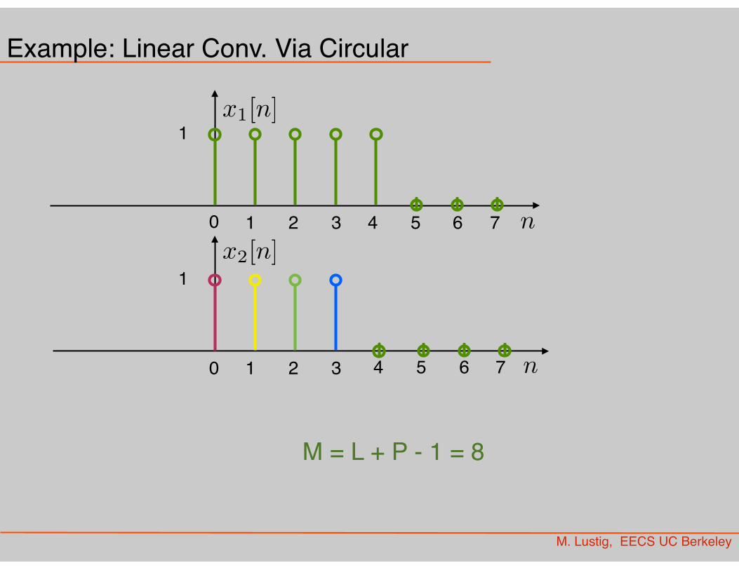
Example: Linear Conv. Via Circular
n0 1 2 3 4
1
n0 1 2
1
3
M = L + P - 1 = 8
6 75
4 6 75
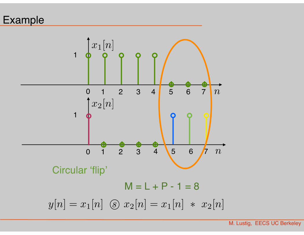
x1[n]
x2[n]
y[n] = x1[n] �8 x2[n] = x1[n] ⇤ x2[n]
M. Lustig, EECS UC Berkeley
Example
n0 1 2 3 4
1
n0 1 2
1
3
M = L + P - 1 = 8
6 75
4 6 75
Circular ‘flip’

M. Lustig, EECS UC Berkeley
Linear Convolution via Circular Convolution
• Zero-pad x[n] by P-1 zeros
• Zero-pad h[n] by L-1 zeros
• Now, both sequences are of length M=L+P-1
xzp[n] =
⇢x[n] 0 n L� 10 L n L+ P � 2
hzp[n] =
⇢h[n] 0 n P � 10 P n L+ P � 2
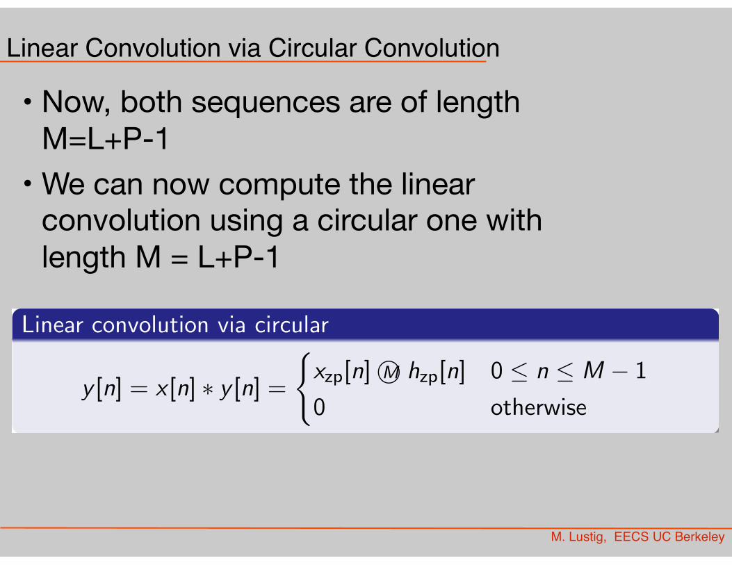
M. Lustig, EECS UC Berkeley
Linear Convolution via Circular Convolution
• Now, both sequences are of length M=L+P-1
• We can now compute the linear convolution using a circular one with length M = L+P-1
Linear Convolution using the DFT
Both zero-padded sequences xzp
[n] and hzp
[n] are of lengthM = L+ P � 1
We can compute the linear convolution x [n] ⇤ h[n] = y [n] bycomputing circular convolution x
zp
[n]�M hzp
[n]:
Linear convolution via circular
y [n] = x [n] ⇤ y [n] =(xzp
[n]�M hzp
[n] 0 n M � 1
0 otherwise
Miki Lustig UCB. Based on Course Notes by J.M Kahn Fall 2012, EE123 Digital Signal Processing

• In practice we can implement a circulant convolution using the DFT property:
M. Lustig, EECS UC Berkeley
Linear Convolution using DFT
x[n] ⇤ h[n] = xzp[n]�M hzp[n]
= DFT �1 {DFT {xzp[n]} · DFT {hzp[n]}}
for 0 ≤ n ≤ M-1, M=L+P-1
• Advantage: DFT can be computed with Nlog2N complexity (FFT algorithm later!)
• Drawback: Must wait for all the samples -- huge delay -- incompatible with real-time
M. Lustig, EECS UC Berkeley
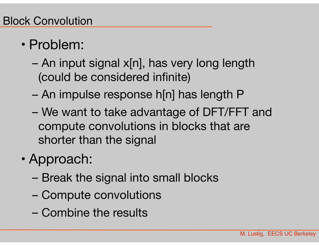
Block Convolution
• Problem: – An input signal x[n], has very long length (could be considered infinite)
– An impulse response h[n] has length P– We want to take advantage of DFT/FFT and compute convolutions in blocks that are shorter than the signal
• Approach:– Break the signal into small blocks– Compute convolutions– Combine the results
M. Lustig, EECS UC Berkeley
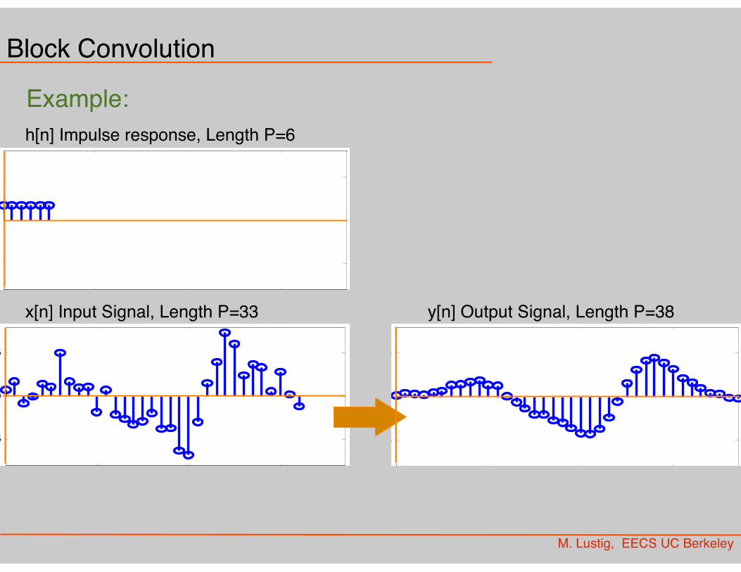
Block Convolution
Example:
0 10 20 30
-0.5
0
0.5
n
x[n]
Input Signal, Length 33
0 10 20 30
-0.5
0
0.5
n
h[n]
Impulse Response, Length P = 6
0 10 20 30
-0.5
0
0.5
n
y[n]
Linear Convolution, Length 38
Miki Lustig UCB. Based on Course Notes by J.M Kahn Fall 2012, EE123 Digital Signal Processing
Block Convolution
Example:
0 10 20 30
-0.5
0
0.5
n
x[n]
Input Signal, Length 33
0 10 20 30
-0.5
0
0.5
n
h[n]
Impulse Response, Length P = 6
0 10 20 30
-0.5
0
0.5
n
y[n]
Linear Convolution, Length 38
Miki Lustig UCB. Based on Course Notes by J.M Kahn Fall 2012, EE123 Digital Signal Processing
Block Convolution
Example:
0 10 20 30
-0.5
0
0.5
n
x[n]
Input Signal, Length 33
0 10 20 30
-0.5
0
0.5
n
h[n]
Impulse Response, Length P = 6
0 10 20 30
-0.5
0
0.5
n
y[n]
Linear Convolution, Length 38
Miki Lustig UCB. Based on Course Notes by J.M Kahn Fall 2012, EE123 Digital Signal Processing
h[n] Impulse response, Length P=6
x[n] Input Signal, Length P=33 y[n] Output Signal, Length P=38
Block Convolution
Example:
M. Lustig, EECS UC Berkeley
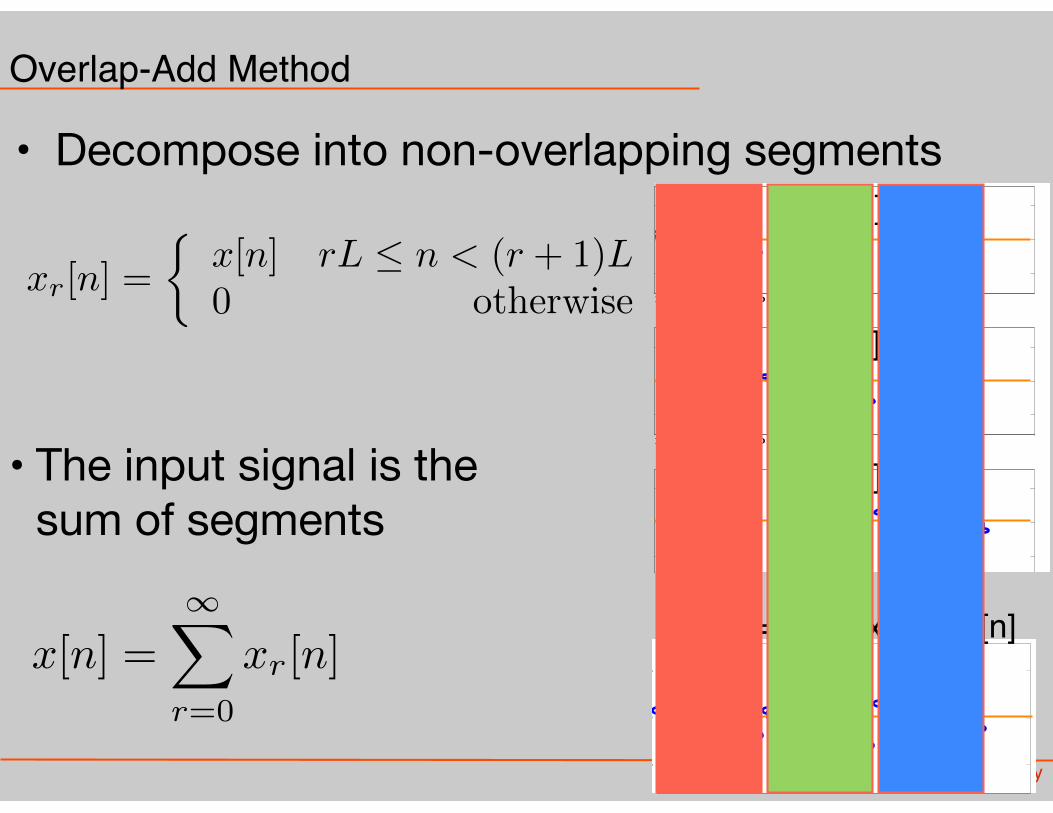
Overlap-Add Method
• Decompose into non-overlapping segmentsOverlap-Add Method
0 10 20 30
-0.5
0
0.5
n
x 0[n]
Overlap-Add, Input Segments, Length L = 11
0 10 20 30
-0.5
0
0.5
n
y 0[n]
Overlap-Add, Output Segments, Length L+P-1 = 16
0 10 20 30
-0.5
0
0.5
n
x 1[n]
0 10 20 30
-0.5
0
0.5
n
y 1[n]
0 10 20 30
-0.5
0
0.5
n
x 2[n]
0 10 20 30
-0.5
0
0.5
n
y 2[n]
0 10 20 30
-0.5
0
0.5
n
x[n]
Overlap-Add, Sum of Input Segments
0 10 20 30
-0.5
0
0.5
n
y[n]
Overlap-Add, Sum of Output Segments
Miki Lustig UCB. Based on Course Notes by J.M Kahn Fall 2012, EE123 Digital Signal Processing
Block Convolution
Example:
0 10 20 30
-0.5
0
0.5
n
x[n]
Input Signal, Length 33
0 10 20 30
-0.5
0
0.5
nh[n]
Impulse Response, Length P = 6
0 10 20 30
-0.5
0
0.5
n
y[n]
Linear Convolution, Length 38
Miki Lustig UCB. Based on Course Notes by J.M Kahn Fall 2012, EE123 Digital Signal Processing
x0[n]
x1[n]
x2[n]
x[n] = x0[n]+x1[n]+x2[n]
xr[n] =
⇢x[n] rL n < (r + 1)L
0 otherwise
• The input signal is the sum of segments
x[n] =1X
r=0
xr[n]
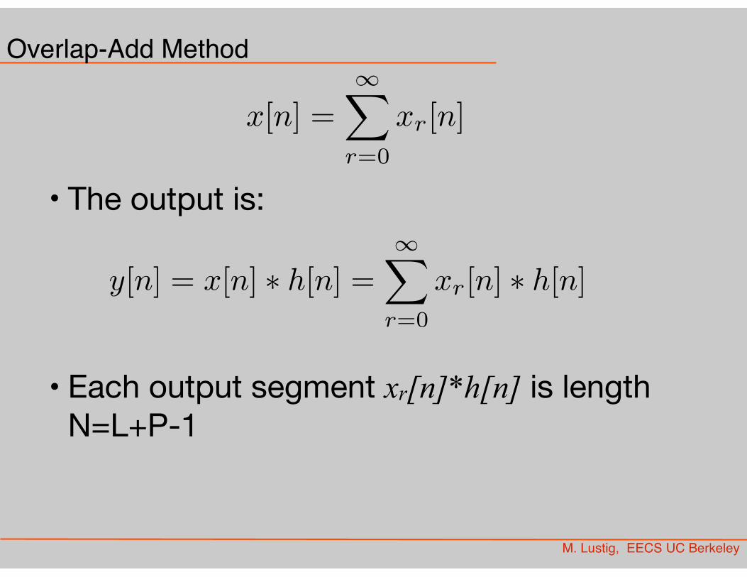
M. Lustig, EECS UC Berkeley
Overlap-Add Method
• The output is:
• Each output segment xr[n]*h[n] is length N=L+P-1
x[n] =1X
r=0
xr[n]
y[n] = x[n] ⇤ h[n] =1X
r=0
xr[n] ⇤ h[n]
M. Lustig, EECS UC Berkeley
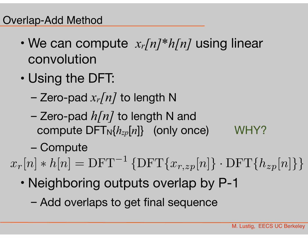
Overlap-Add Method
• We can compute xr[n]*h[n] using linear convolution
• Using the DFT:– Zero-pad xr[n] to length N– Zero-pad h[n] to length N and compute DFTN{hzp[n]} (only once) WHY?
– Compute
• Neighboring outputs overlap by P-1– Add overlaps to get final sequence
xr[n] ⇤ h[n] = DFT�1 {DFT{xr,zp[n]} ·DFT{hzp[n]}}
Overlap-Add Method
0 10 20 30
-0.5
0
0.5
n
x 0[n]
Overlap-Add, Input Segments, Length L = 11
0 10 20 30
-0.5
0
0.5
n
y 0[n]
Overlap-Add, Output Segments, Length L+P-1 = 16
0 10 20 30
-0.5
0
0.5
n
x 1[n]
0 10 20 30
-0.5
0
0.5
n
y 1[n]
0 10 20 30
-0.5
0
0.5
n
x 2[n]
0 10 20 30
-0.5
0
0.5
n
y 2[n]
0 10 20 30
-0.5
0
0.5
n
x[n]
Overlap-Add, Sum of Input Segments
0 10 20 30
-0.5
0
0.5
n
y[n]
Overlap-Add, Sum of Output Segments
Miki Lustig UCB. Based on Course Notes by J.M Kahn Fall 2012, EE123 Digital Signal Processing
Block Convolution
Example:
0 10 20 30
-0.5
0
0.5
n
x[n]
Input Signal, Length 33
0 10 20 30
-0.5
0
0.5
n
h[n]
Impulse Response, Length P = 6
0 10 20 30
-0.5
0
0.5
n
y[n]
Linear Convolution, Length 38
Miki Lustig UCB. Based on Course Notes by J.M Kahn Fall 2012, EE123 Digital Signal Processing
Block Convolution
Example:
0 10 20 30
-0.5
0
0.5
n
x[n]
Input Signal, Length 33
0 10 20 30
-0.5
0
0.5
n
h[n]
Impulse Response, Length P = 6
0 10 20 30
-0.5
0
0.5
n
y[n]
Linear Convolution, Length 38
Miki Lustig UCB. Based on Course Notes by J.M Kahn Fall 2012, EE123 Digital Signal Processing
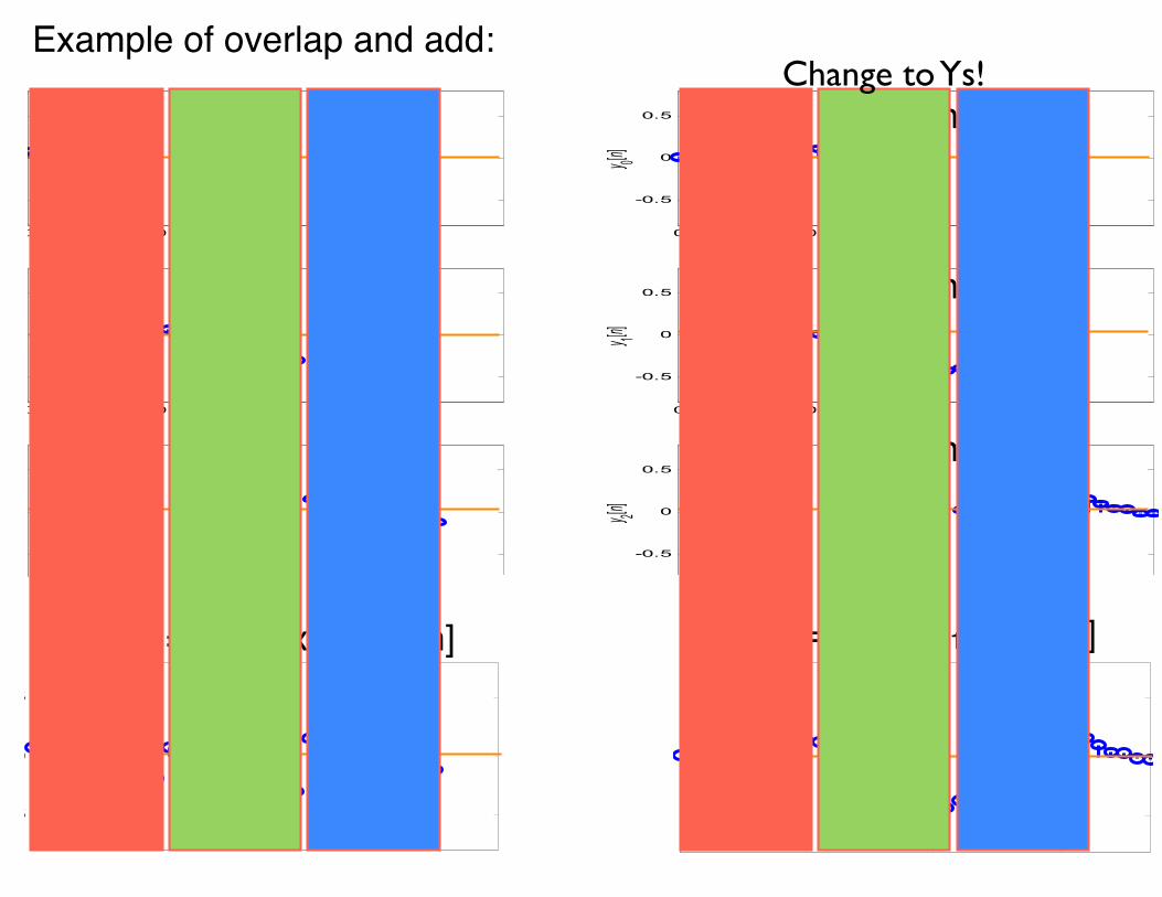
x0[n]
x1[n]
x2[n]
x[n] = x0[n]+x1[n]+x2[n] y[n] = y0[n]+y1[n]+y2[n]
x0[n]
x1[n]
x2[n]
Example of overlap and add:Change to Ys!

M. Lustig, EECS UC Berkeley
Overlap-Save Method
• Basic idea:• Split input into (P-1) overlapping segments
with length L+P-1
• Perform circular convolution in each segment, and keep the L sample portion which is a valid linear convolution
xr[n] =
⇢x[n] rL n < (r + 1)L+ P
0 otherwise
M. Lustig, EECS UC Berkeley
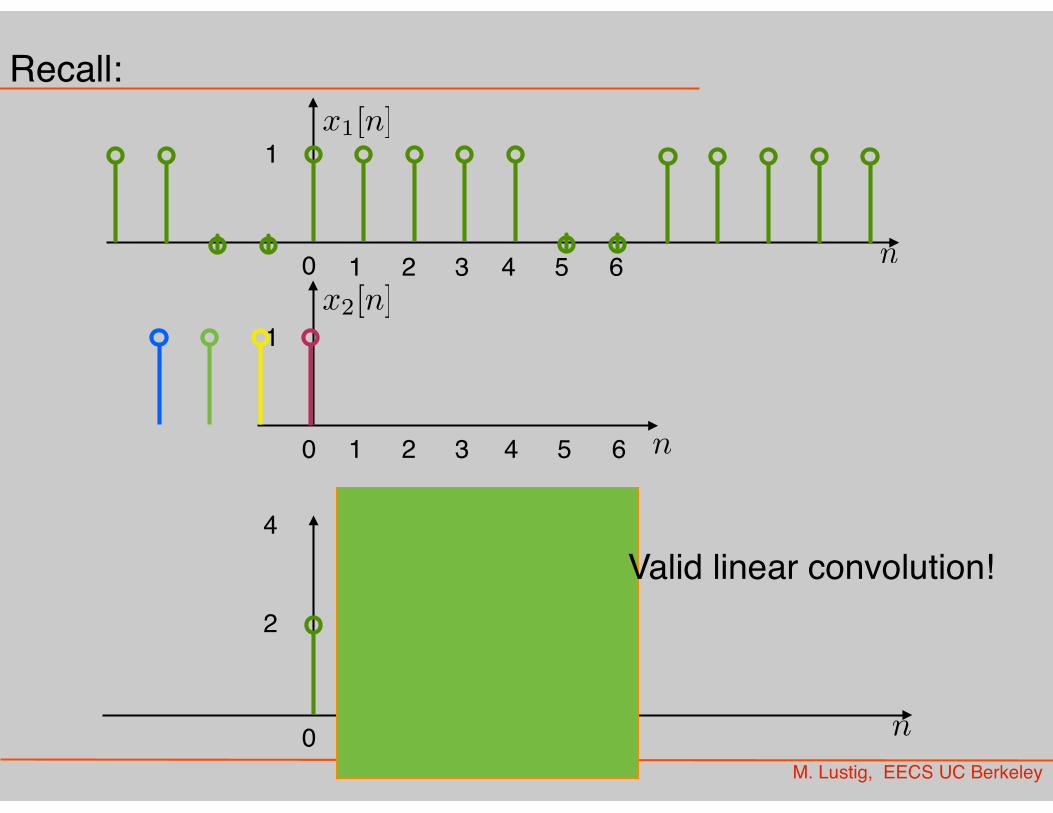
Recall:x1[n]
x2[n]
n0 1 2 3 4
1
n0 1 2
1
5 6
3 4 5 6
n0 1 2 3 4
2
5 6
4Valid linear convolution!

Overlap-Save Method
0 10 20 30
-0.5
0
0.5
n
y[n]
Overlap-Save, Concatenation of Usable Output Segments
0 10 20 30
-0.5
0
0.5
n
x 0[n]
Overlap-Save, Input Segments, Length L = 16
0 10 20 30
-0.5
0
0.5
n
y 0p[n
]
Overlap-Save, Output Segments, Usable Length L - P + 1
Usable (y0[n])
Unusable
0 10 20 30
-0.5
0
0.5
n
x 1[n]
0 10 20 30
-0.5
0
0.5
n
y 1p[n
]
Usable (y1[n])
Unusable
0 10 20 30
-0.5
0
0.5
n
x 2[n)
0 10 20 30
-0.5
0
0.5
n
y 2p[n
]
Usable (y2[n])
Unusable
Miki Lustig UCB. Based on Course Notes by J.M Kahn Fall 2012, EE123 Digital Signal Processing
Example of overlap and save:


