educational tool for heating user guide - lowex · 1 user-guide for the educational tool for energy...
TRANSCRIPT

1
User-Guide for the Educational Tool for Energy and Exergy analyses ofHeating and Cooling Applications in Buildings
To increase the understanding of exergy flows in buildings and to be able to find possibilitiesfor further improvements in energy utilisation in buildings, an analysis tool has been producedduring ongoing work for the IEA ECBCS Annex 37. Throughout the development, the aimwas to produce a “transparent” tool, easy to understand for the target group of architects andbuilding designers, as a whole. Other requirements were that the exergy analysis approach isto be made clear and the required inputs need to be limited. Today, the Microsoft Excelspreadsheet based tool has two input pages and results are summarised on two additionalpages, with diagrams.
All steps of the energy chain - from the primary energy source, via the building, to the sink(i.e. the ambient environment) - are included in the analysis. The entire tool is built up indifferent blocks of sub-systems for all important steps in the energy chain. All components,building construction parts, and building services equipment, have sophisticated inputpossibilities, as described further down. Heat losses in the different components are regarded,as well as the auxiliary electricity required for pumps and fans. The electricity demand forartificial lighting and for driving fans in the ventilation system is also included. On theprimary energy side, the inputs are differentiated between fossil and renewable sources. Thesteady state calculation for this heating case is done in the direction of the development ofdemand.
Although the analysis follows the same main principles of European Standards do, the tool isaimed at calculations under steady state design condition, not at annual energy usecalculations (the user can enter mean values of climatic data to represent seasonal or annualaverage conditions).
WARNINGS:
It is important to note that the tool is an educational or pedagogic tool to demonstrate theinterest of an exergetic approach, to compare some technical solutions and thus to help thedecision.
It is not an actual “pre-design tool”: for example, one can’t actually adapt case by case thecalculation (e.g. no transient calculation of the load).
As it is an educational tool it could be used to understand the effect of changes of onecomponent of the only heating system or chain, without the additional energy uses or servicesof a building to clearly introduce and demonstrate the exergy approach.
One must note also that the Co-generation (combined Heat and Power generation) is treatedby the tool, by the only for the heat part. The local and proper electricity production is nottaken into account as a gain compared to the network.
The tool mainly presents seven parts of an excel worksheet. These parts are successively:1. Section 1: project data, boundaries2. Section 2: heat losses3. Section 3: heat gains4. Section 4: other uses of auxiliary energy5. Section 5: calculation of the heat demand under design conditions6. Section 6: specification of input data for the building services

2
7. Section 7: the energy / exergy analysis

3
1. Description of the tool ..............................................................................................................................................4- 4 -
2. Presentation of the tool.............................................................................................................................................6- 6 -
2.1 Tool section 1: Project data, boundary conditions .......................................................................................6- 6 -
2.2 Tool section 2: Heat losses ...............................................................................................................................7- 7 -
2.2.1 Transmission heat losses ΦT..................................................................................................................7- 7 -
2.2.2 Ventilation heat losses ΦV......................................................................................................................8- 8 -
2.3 Tool section 3: Heat gains.................................................................................................................................8- 8 -
2.3.1 Solar heat gains ΦS ..................................................................................................................................8- 8 -
2.3.2 Internal heat gains Φi ..............................................................................................................................9- 9 -
2.4 Tool section 4: other uses of auxiliary energy...............................................................................................9- 9 -
2.5 Tool section 5: calculation of the heat demand under design conditions Φh .......................................10- 10 -
2.6 Tool section 6: specification of input data for the building services .....................................................10- 10 -
2.6.1 Input data for the combined primary energy transformation and heat generation ...................10- 10 -
2.6.2 Input data for the heat storage system..............................................................................................11- 11 -
2.6.3 Input data for the heat distribution system......................................................................................12- 12 -
2.6.4 Input data for the heat emission system...........................................................................................12- 12 -
2.7 Tool section 7: the energy / exergy analysis ..............................................................................................13- 13 -
2.7.1 Envelope sub-system, no. 7................................................................................................................13- 13 -
2.7.2 Room air sub-system, no. 6................................................................................................................14- 14 -
2.7.3 Emission and control sub-system, no. 5...........................................................................................14- 14 -
2.7.4 Distribution sub-system, no. 4 ...........................................................................................................14- 14 -
2.7.5 Storage sub-system, no. 3 ...................................................................................................................14- 14 -
2.7.6 Generation sub-system, no. 2.............................................................................................................15- 15 -
2.7.7 Primary energy transformation sub-system, no. 1..........................................................................15- 15 -
2.8 System design check......................................................................................................................................15- 15 -
2.9 Results from the analysis ..............................................................................................................................16- 16 -

4
1. Description of the tool
Although the analysis follows the same main principles of the EnEV and other EuropeanStandards do, the tool is aimed at calculations under steady state design condition, not atannual energy use calculations but the user can enter mean values of climatic data to representseasonal or annual average conditions. The tool is divided up into the following blocks or sub-systems (in direction of the flow of energy):
Figure 1: Energy utilisation in building services equipment, the modelling method for the tool.The energy flows are shown from source to sink, in accordance to DIN 4701-10, modified.
1. Primary energy transformation:Sources of energy and the related energy carrier have to be extracted and transformedto a suitable form to be used in buildings. In this regard, the transport of the energycarrier requires additional energy. All these processes are combined and taken intoconsideration in the first block. It is possible to take the environmental aspect ofenergy utilisation (like CO2 emissions) into account in this analysis as renewableenergy sources are treated separately from fossil ones. See chapter 2.7.72.7.7?2.7.7..This is particularly important for electricity generation and transport which representhigh losses.
2. Generation:Bought or final energy enters the boundary of the building. In the case of heating, theenergy carrier (e.g. oil, LNG (liquefied natural gas) or electricity) has to betransformed into heat. This is typically carried out by a combustion process in a boiler.For this process the boiler normally requires some extra auxiliary energy (electricity)and heat losses occur due to non-ideal equipment. For the case of cooling, the boilerhas to be replaced by a chiller, but this case is not regarded in this paper. See chapter2.7.62.7.6?2.7.6. .
3. Storage:Some plant layouts include a heat storage. Here, the storage is characterised by itsspecific heat losses and if needed, its demand on auxiliary energy. Since thecalculation is based on steady state conditions, the advantage of a heat storage can notbe taken into consideration, as would be possible in dynamic calculations. See chapter2.7.52.7.5?2.7.5. .

5
4. Distribution:The heat generated in the boiler and perhaps stored in the storage has to be transportedto the emission system via a distribution system. For waterborne systems, pipes arelaid in walls and ceilings to the emission system. Depending of the insulation standardof the pipes, heat losses occur and auxiliary energy may even be required. See chapter2.7.42.7.4?2.7.4. .
5. Emission:Typical emission systems are radiators, floor heating systems and fan coil units. In thiscase the heat, transported to the emission system, is transferred to the room to beconditioned. Depending on the system design, heat losses may occur and additionalauxiliary energy is required. See chapter 2.7.32.7.3?2.7.3. .
6. Room air:Heat enters the room at the surface of the emission system at a slightly highertemperature than the mean temperature of the room. No heat losses occur at this point,but since the temperature level changes, heat is dissipated into a room, the exergycontent will change. See chapter 2.7.22.7.2?2.7.2. .
7. Envelope:All heat flows leave the building via its envelope, transmission and ventilation losses.In this sub-system, the total dissipation of all heat at a higher temperature level thanthat of the final sink, the outside environment is regarded. See chapter 2.7.12.7.1?2.7.1.

6
2. Presentation of the toolThe first rows, or heading, of the worksheet present the tool.
Educational Tool for an exergyoptimised building design
IEA ECBCS Annex 37 Steady state calculations
for heating casesVersion 2.3
The last rows of the Excel sheet, after calculations, results and diagrams, mention thecollaborators that participated to produce the tool and their addresses.
Authors:Dietrich Schmidt Masanori Shukuya Abdelaziz Hammache Johann Zirngbl & Claude FrancoisKTH Building Technology Musashi Institute of Technology Natural Resources Canada CSTB - Energy Systems and EnvironmentBrinellvägen 34 1-28-1 Tamazutsumi Setagaya-ku 1615 Lionel-Boulet 84 avenue Jean JaurèsS-10044 Stockholm Tokyo 158-8557 Varennes Quebec J3X 1S6 F-77421 Marne-la-Vallée Cedex 2SWEDEN JAPAN CANADA FRANCE
With kind support of Kirsten Höttges; Dep. of Building Physics; University of Kassel; D-34109 Kassel; GERMANY
The row following the heading presents as “Object” the Project Name entered by the user orchosen by him in a set of cases, or Demoprojects, proposed on the right side of the sheet, by aclick on a button.
Object: The ZUB Office Building, IEA Annex 37 Demoproject
The example presented hereafter is the ZUB Office Building. The different lines of sheet andsteps of the calculations are detailed.
The user has to fill in specially the yellow cells of the sheet.The spreadsheet is divided into six different sections for the input and calculation of values(see Appendix A for the complete example and worksheet).Project data and boundary conditions for the analysis are questioned in the first section.In tool section 2, which follows, the heat losses due to transmission through the buildingenvelope and ventilation are estimated.Tool sections 3 and 4 follow, with the estimation of the possible heat gain, both solar andinternal, which are to be subtracted from the heat loss.Tool section 5 sums up the loss and gain, and a heat balance according to the first law ofthermodynamics is set up.The choices for the building service equipment for heating are made in tool section 6. TheEnergy sources, i.e. the boiler / the heat generation part and the actual emission system mustbe chosen.
In tool section 7 the exergy analysis is finally drawn out. All sections are described in moredetail in the following chapter:
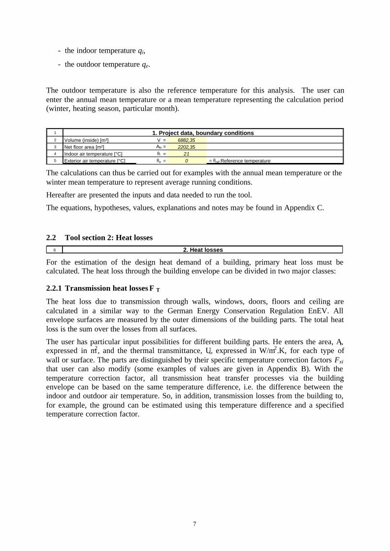
2.1 Tool section 1: Project data, boundary conditions
In this first section, as general project data and design conditions, the user enters:
- the internal volume of the building V,
- the net floor area AN,
7
- the indoor temperature θi,
- the outdoor temperature θe.
The outdoor temperature is also the reference temperature for this analysis. The user canenter the annual mean temperature or a mean temperature representing the calculation period(winter, heating season, particular month).
1
2 Volume (inside) [m³] V = 6882,353 Net floor area [m²] AN = 2202,354 Indoor air temperature [°C] θi = 215 Exterior air temperature [°C] θe = 0 = θref Reference temperature
1. Project data, boundary conditions
The calculations can thus be carried out for examples with the annual mean temperature or thewinter mean temperature to represent average running conditions.
Hereafter are presented the inputs and data needed to run the tool.
The equations, hypotheses, values, explanations and notes may be found in Appendix C.
2.2 Tool section 2: Heat losses6 2. Heat losses
For the estimation of the design heat demand of a building, primary heat loss must becalculated. The heat loss through the building envelope can be divided in two major classes:
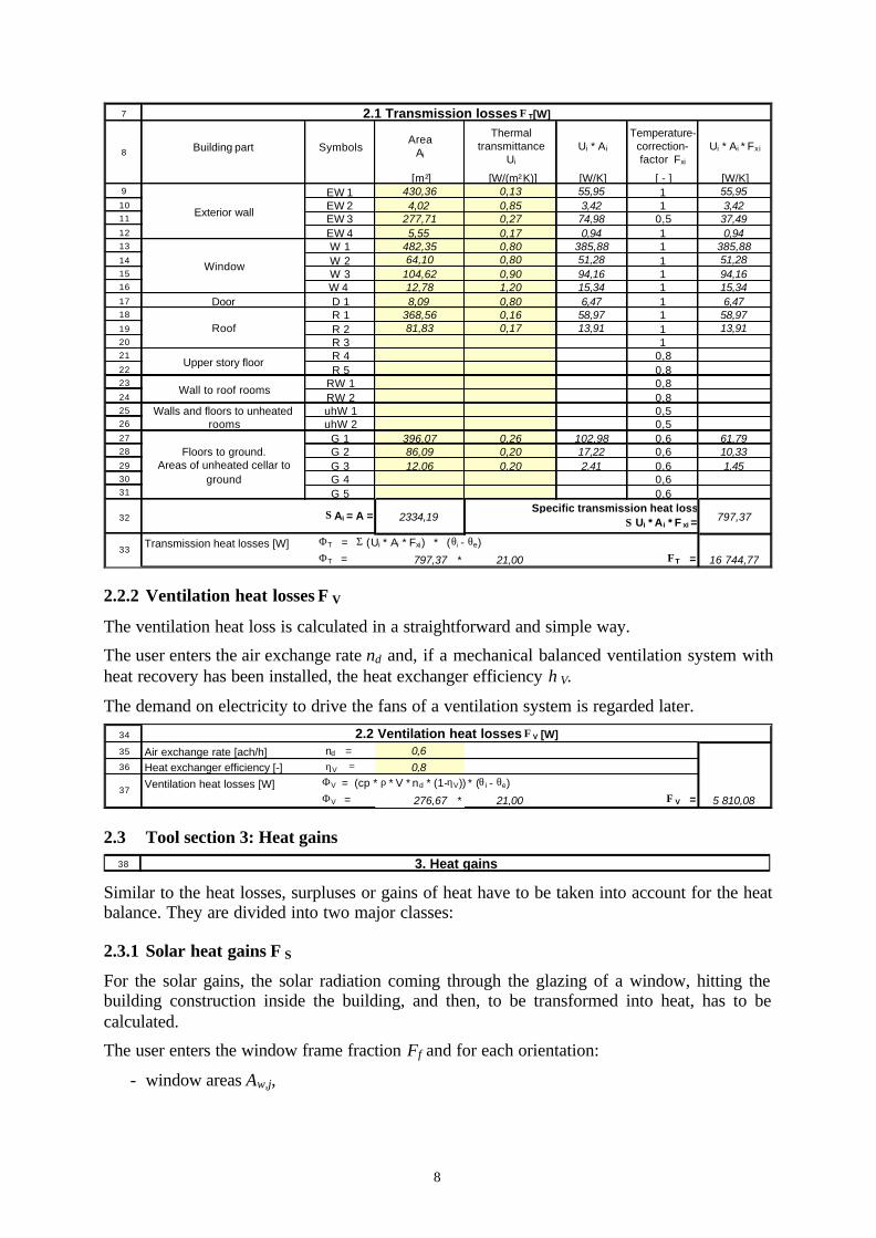
2.2.1 Transmission heat losses Φ T
The heat loss due to transmission through walls, windows, doors, floors and ceiling arecalculated in a similar way to the German Energy Conservation Regulation EnEV. Allenvelope surfaces are measured by the outer dimensions of the building parts. The total heatloss is the sum over the losses from all surfaces.
The user has particular input possibilities for different building parts. He enters the area, Ai,expressed in m2, and the thermal transmittance, Ui, expressed in W/m2.K, for each type ofwall or surface. The parts are distinguished by their specific temperature correction factors Fxithat user can also modify (some examples of values are given in Appendix B). With thetemperature correction factor, all transmission heat transfer processes via the buildingenvelope can be based on the same temperature difference, i.e. the difference between theindoor and outdoor air temperature. So, in addition, transmission losses from the building to,for example, the ground can be estimated using this temperature difference and a specifiedtemperature correction factor.
8
7
Building part SymbolsArea
Ai
Thermal transmittance
Ui
Ui * Ai
Temperature-correction-factor Fxi
Ui * Ai * Fxi
[m²] [W/(m²K)] [W/K] [ - ] [W/K]9 EW 1 430,36 0,13 55,95 1 55,9510 EW 2 4,02 0,85 3,42 1 3,4211 EW 3 277,71 0,27 74,98 0,5 37,4912 EW 4 5,55 0,17 0,94 1 0,9413 W 1 482,35 0,80 385,88 1 385,8814 W 2 64,10 0,80 51,28 1 51,2815 W 3 104,62 0,90 94,16 1 94,1616 W 4 12,78 1,20 15,34 1 15,3417 Door D 1 8,09 0,80 6,47 1 6,4718 R 1 368,56 0,16 58,97 1 58,9719 R 2 81,83 0,17 13,91 1 13,9120 R 3 121 R 4 0,822 R 5 0,823 RW 1 0,824 RW 2 0,825 uhW 1 0,526 uhW 2 0,527 G 1 396,07 0,26 102,98 0,6 61,7928 G 2 86,09 0,20 17,22 0,6 10,3329 G 3 12,06 0,20 2,41 0,6 1,4530 G 4 0,631 G 5 0,6
32 2334,19 797,37
Transmission heat losses [W] ΦT = Σ (Ui * Ai * Fxi) * (θi - θe) ΦT = 797,37 * 21,00 ΦT = 16 744,77
Specific transmission heat loss Σ Ui * Ai * F xi =
2.1 Transmission losses ΦT[W]
Upper story floor
8
Exterior wall
Window
Roof
Wall to roof rooms
Walls and floors to unheated rooms
Floors to ground.Areas of unheated cellar to
ground
Σ Ai = A =
33
2.2.2 Ventilation heat losses ΦV
The ventilation heat loss is calculated in a straightforward and simple way.
The user enters the air exchange rate nd and, if a mechanical balanced ventilation system withheat recovery has been installed, the heat exchanger efficiency ηV.
The demand on electricity to drive the fans of a ventilation system is regarded later.34
35 Air exchange rate [ach/h] nd = 0,636 Heat exchanger efficiency [-] ηV = 0,8
Ventilation heat losses [W] ΦV = 276,67 * 21,00 ΦV = 5 810,08
ΦV = (cp * ρ * V * nd * (1-ηV)) * (θ i - θe) 37
2.2 Ventilation heat losses ΦV [W]
2.3 Tool section 3: Heat gains38 3. Heat gains
Similar to the heat losses, surpluses or gains of heat have to be taken into account for the heatbalance. They are divided into two major classes:
2.3.1 Solar heat gains ΦS
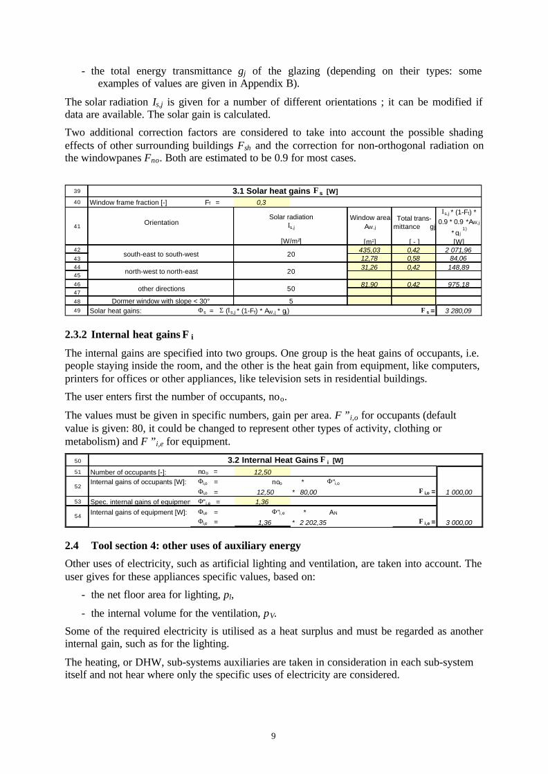
For the solar gains, the solar radiation coming through the glazing of a window, hitting thebuilding construction inside the building, and then, to be transformed into heat, has to becalculated.
The user enters the window frame fraction Ff and for each orientation:
- window areas Aw,j,
9
- the total energy transmittance gj of the glazing (depending on their types: someexamples of values are given in Appendix B).
The solar radiation Is,j is given for a number of different orientations ; it can be modified ifdata are available. The solar gain is calculated.
Two additional correction factors are considered to take into account the possible shadingeffects of other surrounding buildings Fsh and the correction for non-orthogonal radiation onthe windowpanes Fno. Both are estimated to be 0.9 for most cases.
39
40 Window frame fraction [-] Ff = 0,3
Window area AW,j
Total trans-mittance gj
Ιs,j * (1-Ff) * 0.9 * 0.9 *AW,j
* g j 1)
[m²] [ - ] [W]42 435,03 0,42 2 071,9643 12,78 0,58 84,0644 31,26 0,42 148,8945
46 81,90 0,42 975,1847
48
49 Solar heat gains: Φs = Σ (Ιs,j * (1-Ff) * AW,j * gj) Φs = 3 280,09Dormer window with slope < 30°
north-west to north-east 20
5
50
41
3.1 Solar heat gains Φs [W]
south-east to south-west 20
OrientationSolar radiation
Ιs,j
[W/m²]
other directions
2.3.2 Internal heat gains Φi
The internal gains are specified into two groups. One group is the heat gains of occupants, i.e.people staying inside the room, and the other is the heat gain from equipment, like computers,printers for offices or other appliances, like television sets in residential buildings.
The user enters first the number of occupants, noo.
The values must be given in specific numbers, gain per area. Φ”i,o for occupants (defaultvalue is given: 80, it could be changed to represent other types of activity, clothing ormetabolism) and Φ”i,e for equipment.
50
51 Number of occupants [-]: noo = 12,50Internal gains of occupants [W]: Φi,o = noo * Φ"i,o
Φi,o = 12,50 * 80,00 Φi,o = 1 000,0053 Spec. internal gains of equipment [W/m²]: Φ" i,e = 1,36
Internal gains of equipment [W]: Φi,e = Φ"i,e * AN
Φi,e = 1,36 * 2 202,35 Φi,e = 3 000,00
52
3.2 Internal Heat Gains Φ i [W]
54
2.4 Tool section 4: other uses of auxiliary energy
Other uses of electricity, such as artificial lighting and ventilation, are taken into account. Theuser gives for these appliances specific values, based on:
- the net floor area for lighting, pl,
- the internal volume for the ventilation, pV.
Some of the required electricity is utilised as a heat surplus and must be regarded as anotherinternal gain, such as for the lighting.
The heating, or DHW, sub-systems auxiliaries are taken in consideration in each sub-systemitself and not hear where only the specific uses of electricity are considered.
10
55
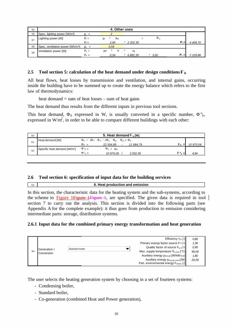
56 Spec. lighting power [W/m²]: pl = 2Lighting power [W]: Pl = pl * AN = Φi,l
Pl = 2,00 * 2 202,35 Pl = 4 404,7058 Spec. ventilation power [Wh/m³]: pv = 0,54
Ventilation power [W]: Pv = pv * V * nd
Pv = 0,54 * 6 882,35 * 0,60 Pv = 2 229,88
4. Other uses
57
59
2.5 Tool section 5: calculation of the heat demand under design conditions Φh
All heat flows, heat losses by transmission and ventilation, and internal gains, occurringinside the building have to be summed up to create the energy balance which refers to the firstlaw of thermodynamics:
heat demand = sum of heat losses – sum of heat gains
The heat demand thus results from the different inputs in previous tool sections.
This heat demand, Φh expressed in W, is usually converted in a specific number, Φ”h,expressed in W/m2, in order to be able to compare different buildings with each other:
60
Heat demand [W]: Φh = (ΦΤ + ΦV) − (Φs + Φi,o + Φi,e + Φi,l)Φh = 22 554,85 - 11 684,79 Φh = 10 870,06
Specific heat demand [W/m²] Φ''h = Φh / AN
Φ''h = 10 870,06 / 2 202,35 Φ''h = 4,94
5. Heat demand Φh [W]
61
62
2.6 Tool section 6: specification of input data for the building services63 6. Heat production and emission
In this section, the characteristic data for the heating system and the sub-systems, according tothe scheme in Figure 1Figure 1Figure 1, are specified. The given data is required in toolsection 7 to carry out the analysis. This section is divided into the following parts (seeAppendix A for the complete example): it thus goes from production to emission consideringintermediate parts: storage, distribution systems.
2.6.1 Input data for the combined primary energy transformation and heat generation
Efficiency ηG [-] 0,80Primary energy factor source F P [-] 1,30
Quality factor of source Fq,S [-] 0,95Max. supply temperature θS,max [°C] 90,00
Auxiliary energy paux,ge [W/kW heat] 1,80Auxiliary energy paux,ge,const [W] 20,00
Part. environmental energy Frenew [-]
64Generation / Conversion:
Standard boiler
The user selects the heating generation system by choosing in a set of fourteen systems:- Condensing boiler,- Standard boiler,- Co-generation (combined Heat and Power generation),

11
- Electric boiler,- Heat pump exhaust air/water,- Heat pump borehole water/glycol,- Heat pump external air/air,- Air heat pump,- Ground heat pump water/water,- Solar collector, flat plate,- Solar collector, vacuum tube,- Bio-mass/Wood,- District heat,- District heat/Waste heat.
For each energy source, the primary energy transformation is characterized by the primaryenergy factor FP and for the exergy analysis the quality factor of the energy source Fq,s. Afraction factor for the environmental energy Frenew takes into account the fossil part saved bythe renewable part of the required primary energy. At each energy source and heatinggeneration system is associated a set of values for these different parameters:
- Efficiency ηG (-)
- Primary energy factor FP (-)
- Quality factor of source Fq,S (-)
- Max. supply temperature θS,max (°C)
- Auxiliary power paux,ge (W/kWheat)
- Auxiliary power (const.) paux,ge,const (W)
- part of environmental energy Frenew (-)
2.6.2 Input data for the heat storage system
The user selects the heat storage system between three possibilities or types:- No storage,- Small / day storage,- Seasonal storage.
The heat storage system is characterised in round terms by:- ηS (-), storage efficiency:- paux,S (W/kWheat), auxiliary power: auxiliary power needed to run the storage, like
electricity needed to drive pumps.- FS (-), solar fraction.
Heat loss / efficiency ηS [-] 1,00Auxiliary energy paux,S [W/kW heat]
Solar fraction FS [-]Storage:65 No storage
12
The seasonal storage in the tool is associated to a solar heating with earth pit storage system.For this special storage a fraction of the overall heating load is assumed to be covered bythermal solar power with a typical fraction for these systems of 40 %.
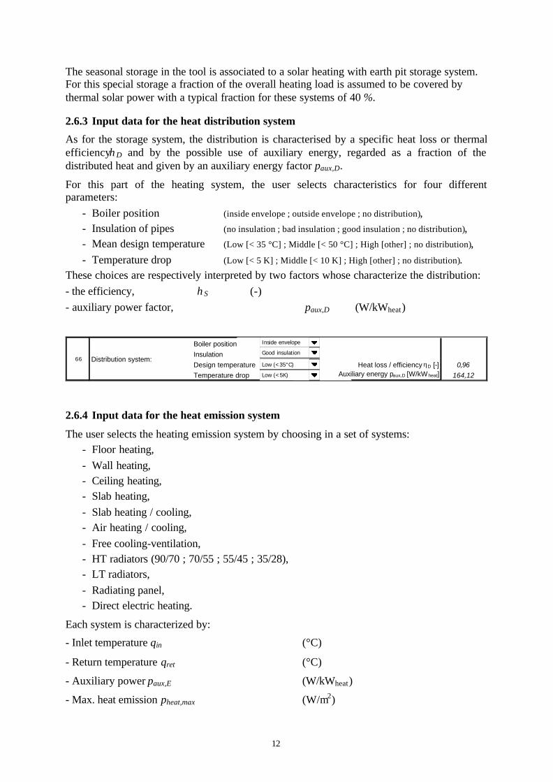
2.6.3 Input data for the heat distribution system
As for the storage system, the distribution is characterised by a specific heat loss or thermalefficiencyηD and by the possible use of auxiliary energy, regarded as a fraction of thedistributed heat and given by an auxiliary energy factor paux,D.
For this part of the heating system, the user selects characteristics for four differentparameters:
- Boiler position (inside envelope ; outside envelope ; no distribution),- Insulation of pipes (no insulation ; bad insulation ; good insulation ; no distribution),- Mean design temperature (Low [< 35 °C] ; Middle [< 50 °C] ; High [other] ; no distribution),- Temperature drop (Low [< 5 K] ; Middle [< 10 K] ; High [other] ; no distribution).
These choices are respectively interpreted by two factors whose characterize the distribution:- the efficiency, ηS (-)- auxiliary power factor, paux,D (W/kWheat)
Boiler positionInsulationDesign temperature Heat loss / efficiency ηD [-] 0,96Temperature drop Auxiliary energy paux,D [W/kW heat] 164,12
66 Distribution system:
Inside envelope
Good insulation
Low (<35°C)
Low (<5K)
2.6.4 Input data for the heat emission system
The user selects the heating emission system by choosing in a set of systems:- Floor heating,- Wall heating,- Ceiling heating,- Slab heating,- Slab heating / cooling,- Air heating / cooling,- Free cooling-ventilation,- HT radiators (90/70 ; 70/55 ; 55/45 ; 35/28),- LT radiators,- Radiating panel,- Direct electric heating.
Each system is characterized by:
- Inlet temperature θin (°C)
- Return temperature θret (°C)
- Auxiliary power paux,E (W/kWheat)
- Max. heat emission pheat,max (W/m2)
13
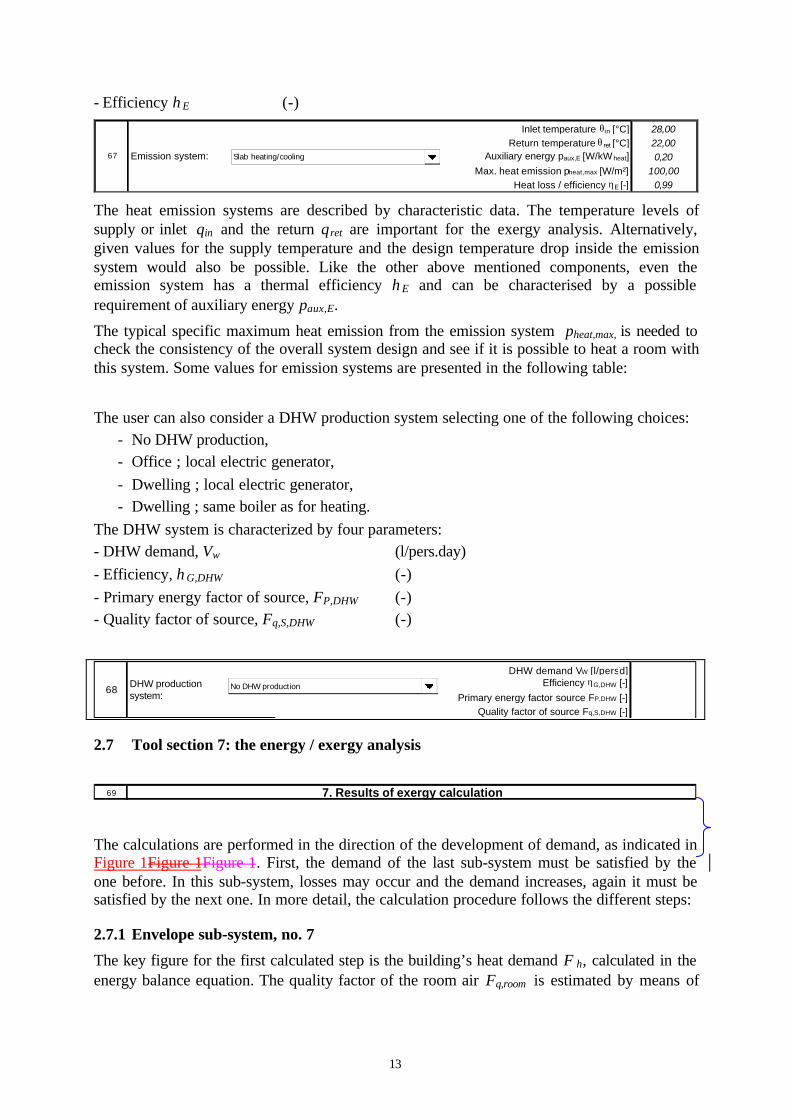
- Efficiency ηE (-)
Inlet temperature θin [°C] 28,00Return temperature θ ret [°C] 22,00
Auxiliary energy paux,E [W/kW heat] 0,20Max. heat emission pheat,max [W/m²] 100,00
Heat loss / efficiency ηE [-] 0,99
67 Emission system: Slab heating/cooling
The heat emission systems are described by characteristic data. The temperature levels ofsupply or inlet θin and the return θret are important for the exergy analysis. Alternatively,given values for the supply temperature and the design temperature drop inside the emissionsystem would also be possible. Like the other above mentioned components, even theemission system has a thermal efficiency ηE and can be characterised by a possiblerequirement of auxiliary energy paux,E.
The typical specific maximum heat emission from the emission system pheat,max, is needed tocheck the consistency of the overall system design and see if it is possible to heat a room withthis system. Some values for emission systems are presented in the following table:
The user can also consider a DHW production system selecting one of the following choices:- No DHW production,- Office ; local electric generator,- Dwelling ; local electric generator,- Dwelling ; same boiler as for heating.
The DHW system is characterized by four parameters:- DHW demand, Vw (l/pers.day)- Efficiency, ηG,DHW (-)- Primary energy factor of source, FP,DHW (-)- Quality factor of source, Fq,S,DHW (-)
DHW demand VW [l/pers.d]Efficiency ηG,DHW [-]
Primary energy factor source FP,DHW [-]Quality factor of source Fq,S,DHW [-]
68 DHW production system:
No DHW production
2.7 Tool section 7: the energy / exergy analysis
69 7. Results of exergy calculation
The calculations are performed in the direction of the development of demand, as indicated inFigure 1Figure 1Figure 1. First, the demand of the last sub-system must be satisfied by theone before. In this sub-system, losses may occur and the demand increases, again it must besatisfied by the next one. In more detail, the calculation procedure follows the different steps:
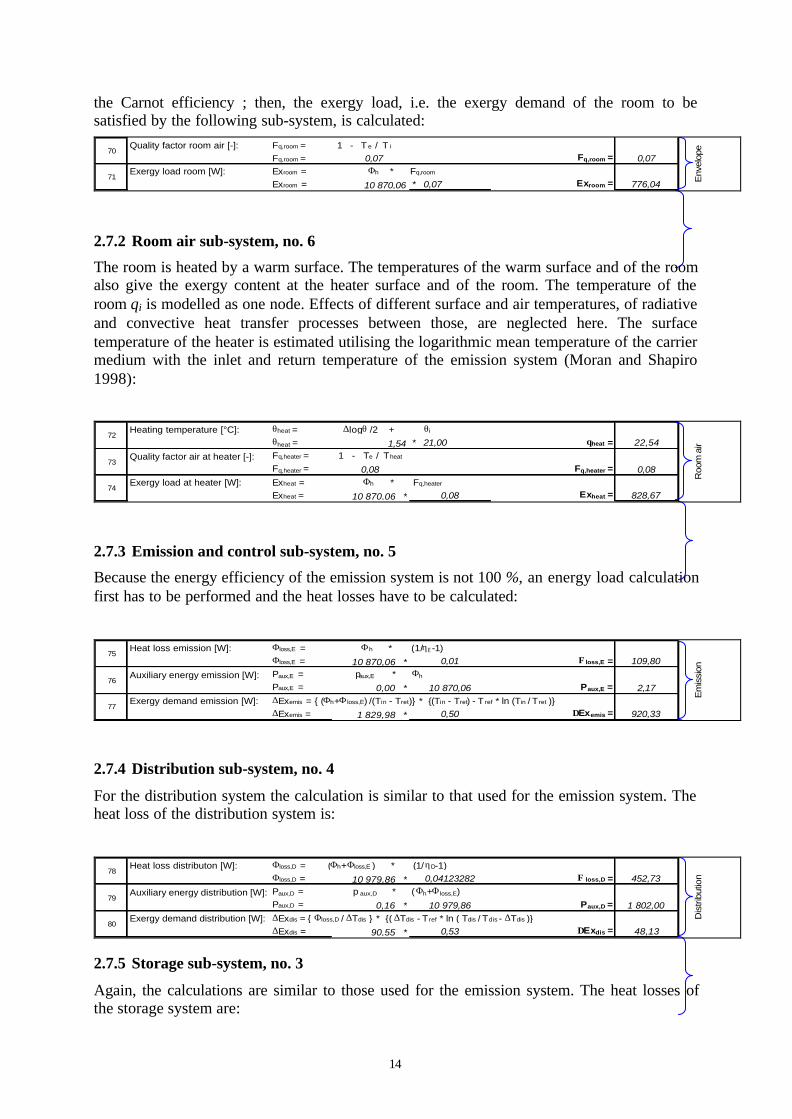
2.7.1 Envelope sub-system, no. 7
The key figure for the first calculated step is the building’s heat demand Φh, calculated in theenergy balance equation. The quality factor of the room air Fq,room is estimated by means of
14
the Carnot efficiency ; then, the exergy load, i.e. the exergy demand of the room to besatisfied by the following sub-system, is calculated:
Quality factor room air [-]: Fq,room = 1 - T e / T i
Fq,room = 0,07 Fq,room = 0,07Exergy load room [W]: Exroom = Φh * Fq,room
Exroom = 10 870,06 * 0,07 Exroom = 776,04 Env
elop
e70
71
2.7.2 Room air sub-system, no. 6
The room is heated by a warm surface. The temperatures of the warm surface and of the roomalso give the exergy content at the heater surface and of the room. The temperature of theroom θi is modelled as one node. Effects of different surface and air temperatures, of radiativeand convective heat transfer processes between those, are neglected here. The surfacetemperature of the heater is estimated utilising the logarithmic mean temperature of the carriermedium with the inlet and return temperature of the emission system (Moran and Shapiro1998):
Heating temperature [°C]: θheat = ∆logθ /2 + θi
θheat = 1,54 * 21,00 θheat = 22,54
Quality factor air at heater [-]: Fq,heater = 1 - Te / Theat
Fq,heater = 0,08 Fq,heater = 0,08Exergy load at heater [W]: Exheat = Φh * Fq,heater
Exheat = 10 870,06 * 0,08 Exheat = 828,6774
72
Roo
m a
ir
73
2.7.3 Emission and control sub-system, no. 5
Because the energy efficiency of the emission system is not 100 %, an energy load calculationfirst has to be performed and the heat losses have to be calculated:
Heat loss emission [W]: Φloss,E = Φh * (1/ηE-1)Φloss,E = 10 870,06 * 0,01 Φloss,E = 109,80
Auxiliary energy emission [W]: Paux,E = paux,E * Φh
Paux,E = 0,00 * 10 870,06 Paux,E = 2,17Exergy demand emission [W]: ∆Exemis = { (Φh+Φ loss,E) /(Tin - Tret)} * {(Tin - Tret) - T ref * ln (Tin / T ret )}
∆Exemis = 1 829,98 * 0,50 ∆Exemis = 920,3377
Em
issi
on
76
75
2.7.4 Distribution sub-system, no. 4
For the distribution system the calculation is similar to that used for the emission system. Theheat loss of the distribution system is:
Heat loss distributon [W]: Φloss,D = (Φh+Φloss,E ) * (1/ηD-1)Φloss,D = 10 979,86 * 0,04123282 Φ loss,D = 452,73
Auxiliary energy distribution [W]: Paux,D = p aux,D * (Φh+Φ loss,E) Paux,D = 0,16 * 10 979,86 Paux,D = 1 802,00
Exergy demand distribution [W]: ∆Exdis = { Φloss,D / ∆Tdis } * {( ∆Tdis - T ref * ln ( Tdis / Tdis - ∆Tdis )}∆Exdis = 90,55 * 0,53 ∆Exdis = 48,13
80
Dis
tribu
tion
78
79
2.7.5 Storage sub-system, no. 3
Again, the calculations are similar to those used for the emission system. The heat losses ofthe storage system are:

15
Heat loss storage [W]: Φloss,S = (Φh+Φ loss,E+Φloss,D) * (1/ηS-1)Φloss,S = 11 432,59 * Φloss,S =
Auxiliary energy storage [W]: Paux,S = paux,S * (Φh+Φloss,E +Φ loss,D) Paux,S = * 11 432,59 Paux,S =
Exergy demand storage [W]: ∆Exstor = { Φloss,S / ∆Tsto } * { ∆Tsto - Tref * ln ( Tdis + ∆Tdis / Tdis + ∆Tdis - ∆Tsto )}∆Exstor = ∆Exstor =
Sto
rage
83
81
82
2.7.6 Generation sub-system, no. 2
The generation sub-system has to satisfy the demands of all previous sub-systems. If aseasonal storage is integrated into the system design, some of the required heat is covered bythermal solar power with a solar fraction FS. The required energy to be covered from thegenerator is:
Req. energy of generation [W]: Φge = (Φh+Φloss,E+Φloss,D+Φ loss,S) * (1-FS) / ηΒ
Φge = 11 432,59 * 1,00 / 0,80 Φge = 14 290,74
Auxiliary energy generation [W]: Paux,ge = paux,ge * (Φh+Φloss,E+Φ loss,D+Φ loss,S) + paus,ge,const
Paux,ge = 0,00 * 11 432,59 + 20,00 Paux,ge = 40,58
Exergy load generation [W]: Exge = ΦGe * Fq,S
Exge = 14 290,74 * 0,95 Exge = 13 576,20
DHW energy demand [W] PW = VW * cp * ρ * ∆T * noo / ηG,DHW
PW = * / PW =
Exergy load plant [W]: Explant = (P l + PV) * Fq,electricity + PW * Fq,s,DHW
Explant = 6 634,58 + Explant = 6 634,58
Gen
erat
ion
86
88
85
84
87
2.7.7 Primary energy transformation sub-system, no. 1
The overall energy and exergy loads of the building are expressed in the required primaryenergy and exergy inputs.
Req. primary energy input [W]: Eprim,tot = Φge * FP + (P I+PV+ΣPaux) * FP,electricity + PW * F P,DHW
Eprim,tot = 18 577,96 + 25 438,01 + Eprim,tot = 44 015,97
Add. renew. energy input [W]: Erenew = Φge * F renew + Eenvironment
Erenew = Erenew =
Total exergy input [W]: Extot = Φge*FP*Fq,S+(P I+PV+ΣPaux)*F P,elec*Fq,elec+PW*FP,DHW*Fq,S,DHW+Erenew*Fq,renew
Extot = 43 087,07 + + Extot = 43 087,0791
89
90
Ene
rgy
trans
form
atio
n
2.8 System design check
The tool automatically checks if the overall system design is consistent. The three differenttests are:
1. If the calculated heat demand is higher than the possible maximum heat output of thesystem, a message will be displayed. New and modern buildings with advancedemission systems, like slab heating, need a suitable building shell because of thelimited heating power output. Thus, a heating system with a higher possible heatoutput should be used or the heating load should be reduced, e.g. by improving theinsulation standard or installing a balanced ventilation with heat recovery.If Nheath Ap ⋅>Φ max, the display will show:”WARNING: Heating power demand is higher than the installed power! The systemsolution is NOT sufficient! Improve building envelope or use a more powerfulsystem”.
16
2. To check if the different components of the heating system have been carefully andcorrectly chosen, the temperature levels are compared. The maximum outputtemperature of the boiler must be higher than the required supply temperature of theemission system.If inS θθ <max, the display will show:”WARNING: Error in system design. Necessary inlet temperature NOT beingsupplied by generation. Change system design”.
3. The tool is made for the calculation of heating cases only. Calculations of cooling caseswould give incorrect results if the heat demand turned out to be negative. Therefore, acheck is included to prevent such results.If ( ) ( )lieioiSVT ,,, Φ+Φ+Φ+Φ<Φ+Φ or 0<Φ h the display will be:”WARNING: Overheating, cooling needed. Apply solar protection, reduce internalloads”.
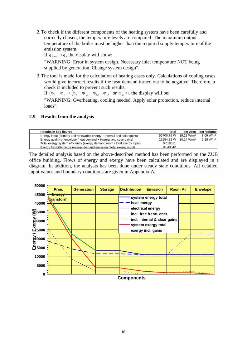
2.9 Results from the analysis
Results in key figures total per Area per VolumeEnergy input (primary and renewable energy + internal and solar gains) 55700,75 W 25,29 W/m² 8,09 W/m³Energy quality of envelope (heat demand + internal and solar gains) 22554,85 W 10,24 W/m² 3,28 W/m³Total exergy system efficiency (exergy demand room / total exergy input) 0,018011Exergy flexibility factor (exergy demand emission / total exergy input) 0,040642
The detailed analysis based on the above-described method has been performed on the ZUBoffice building. Flows of energy and exergy have been calculated and are displayed in adiagram. In addition, the analysis has been done under steady state conditions. All detailedinput values and boundary conditions are given in Appendix A.
0
5000
10000
15000
20000
25000
30000
35000
40000
45000
50000
1 2 3 4 5 6 7 8Components
En
erg
y / E
xerg
y (W
)
system energy totalheat energyelectrical energyincl. free /rene. ener.incl. internal & sloar gainssystem exergy totalexergy incl. gains
Generation Emission Room Air EnvelopeDistributionStoragePrim. Energy
transform

17
Figure 2: Energy and exergy flow through the building service components of the ZUB building. Absolute valuesof energy and exergy flows through all components, from the energy source to the sink, i.e. the externalenvironment. The useable amounts of energy and exergy are reduced in every component due toinefficiencies and losses.
The results are displayed as demands and losses by components. In this diagram, it is easier tounderstand where inefficiencies occur and possible steps for a further increase in the systemefficiency may be indicated.
It is clearly shown that the greatest imperfections occur in two energy transformationcomponents, the primary energy transformation and the heat generation component.
0
5000
10000
15000
20000
25000
Primaryenergy
transform
Generation Storage Distribution Emission Room air Envelope
Components
En
erg
y/E
xerg
y (W
)
rel exergy lossrel energy loss
Figure 3: Exergy losses / demands and energy utilisation by components of the ZUB building. The losses ofuseable energy and the consumption of exergy in every component are shown as bars.
The following diagrams, Figure 4Figure 4Figure 4 and Figure 5Figure 6Figure 5, depict otherpossibilities of where losses happen and system imperfections occur. On the left-hand side ofthe diagrams, the supplies are shown and on the right hand side, the covered demand andlosses are shown. These occur in the indicated places and are covered by shown componentsor sources:

18
0,00
10000,00
20000,00
30000,00
40000,00
50000,00
60000,00
energy gains energy loss
En
erg
y (W
)prim transformDHWventilation eleclightingElectrical energyinefficeint generationsystem heat lossesventilation transmission wallstransmission groundtransmission rooftransmision windowprimary energyrenewableinternalsolar (windows)
Figure 4: Energy supplies / gains and utilisation for the ZUB building
According to the first law of thermodynamics, the supplied energy to a building has to beequal to all losses and needs. Both columns in Figure 4Figure 4Figure 4 show the same endvalue. Again, it is remarkable to realise that the greatest losses occur in the primary energytransformation, in a component that is not itself a building component, but the losses arecaused by the need of the building. The same is true for the results of the exergy analysisshown in Figure 5Figure 6Figure 5. The primary energy transformation is a major part of theexergy flows.

19
0,00
5000,00
10000,00
15000,00
20000,00
25000,00
30000,00
35000,00
40000,00
45000,00
50000,00
exergy supply exergy demand
Exe
rgy
(W)
Primary exergyGenerationStorageDistributionEmissionRoom AirEnvelopeprimary exergyrenewableinternalsolar (windows)
Figure 565:Exergy supply and demands for the ZUB building
Unlike Figure 4Figure 4Figure 4, Figure 5Figure 6Figure 5 shows that the supply column atthe left-hand side and the demand column are not equally high. The exergy supply into abuilding might be higher than the needed demand. Transformation processes may account forthese differences. So, high exergy solar radiation gets through the windows of a building andis then transformed into low exergy heat at the building interior surfaces.
What’s remarkable about this result is the small amount of exergy supply from internalsources, which it is not visible in the graph. The amount of supplied heat energy can beclearly seen in Figure 4Figure 4Figure 4. Another point to observe is the small exergy load ofthe room, the lowest fraction on the right hand side. Only this low level of exergy demand hasto be satisfied by the all heating components inside the building. All transformations andenergy transport processes require more exergy than keeping the room comfortably heated.
Similar to the last two diagrams, gains and losses can be indicated differently. Perhaps themost advanced diagrams which show flows of energy and exergy are Sankey diagrams, aspresented in the following. These Sankey diagrams are not provided by the pre-design tool,but all values.
The user can also run this tool for example to study:
- the impact of improvements in the building envelope versus improvements in theservice equipment,

20
- the system flexibility and the possible integration of renewable energy sources intobuilding systems,
- integration of heat pumps into the building design,
- integration of balanced ventilation systems.
Appendix A
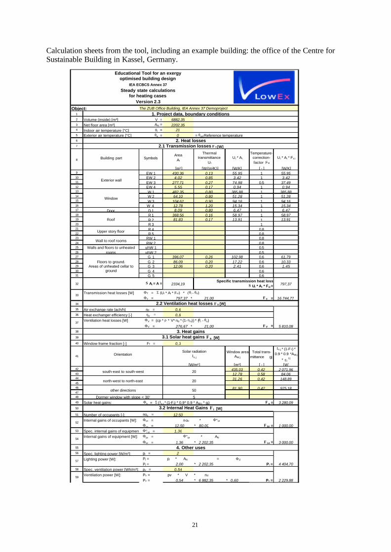
21
Calculation sheets from the tool, including an example building: the office of the Centre forSustainable Building in Kassel, Germany.
Object:1
2 Volume (inside) [m³] V = 6882,353 Net floor area [m²] AN = 2202,354 Indoor air temperature [°C] θi = 215 Exterior air temperature [°C] θe = 0 = θref Reference temperature6
7
Building part SymbolsArea
Ai
Thermal transmittance
U i
U i * Ai
Temperature-correction-factor Fxi
U i * Ai * Fx i
[m² ] [W/(m²K)] [W/K] [ - ] [W/K]9 EW 1 430,36 0,13 55,95 1 55,9510 EW 2 4,02 0,85 3,42 1 3,4211 EW 3 277,71 0,27 74,98 0,5 37,4912 EW 4 5,55 0,17 0,94 1 0,9413 W 1 482,35 0,80 385,88 1 385,8814 W 2 64,10 0,80 51,28 1 51,2815 W 3 104,62 0,90 94,16 1 94,1616 W 4 12,78 1,20 15,34 1 15,3417 Door D 1 8,09 0,80 6,47 1 6,4718 R 1 368,56 0,16 58,97 1 58,9719 R 2 81,83 0,17 13,91 1 13,9120 R 3 121 R 4 0,822 R 5 0,823 RW 1 0,824 RW 2 0,825 uhW 1 0,526 uhW 2 0,527 G 1 396,07 0,26 102,98 0,6 61,7928 G 2 86,09 0,20 17,22 0,6 10,3329 G 3 12,06 0,20 2,41 0,6 1,4530 G 4 0,631 G 5 0,6
32 2334,19 797,37
Transmission heat losses [W] ΦT = Σ (U i * Ai * Fx i) * (θi - θe) ΦT = 797,37 * 21,00 ΦT = 16 744,77
34
35 Air exchange rate [ach/h] nd = 0,636 Heat exchanger efficiency [-] ηV = 0,8
Ventilation heat losses [W]
ΦV = 276,67 * 21,00 ΦV = 5 810,0838
39
40 Window frame fraction [-] Ff = 0,3
Window area AW,j
Total trans-mittance gj
Ιs,j * (1-F f) * 0.9 * 0.9 *AW,j
* gj 1)
[m²] [ - ] [W]42 435,03 0,42 2 071,9643 12,78 0,58 84,0644 31,26 0,42 148,894546 81,90 0,42 975,184748
49 Solar heat gains: Φs = Σ (Ιs,j * (1-F f) * 0,9* 0,9 * AW,j * gj) Φs = 3 280,0950
51 Number of occupants [-]: noo = 12,50Internal gains of occupants [W]: Φi,o = noo * Φ"i,o
Φi,o = 12,50 * 80,00 Φi,o = 1 000,0053 Spec. internal gains of equipment [W/m²]: Φ"i,e = 1,36
Internal gains of equipment [W]: Φi,e = Φ"i,e * AN
Φi,e = 1,36 * 2 202,35 Φi,e = 3 000,0055
56 Spec. lighting power [W/m²]: pl = 2
Lighting power [W]: Pl = pl * AN = Φi,l
Pl = 2,00 * 2 202,35 Pl = 4 404,7058 Spec. ventilation power [Wh/m³]: pv = 0,54
Ventilation power [W]: Pv = pv * V * nd
Pv = 0,54 * 6 882,35 * 0,60 Pv = 2 229,88
33
37
2.2 Ventilation heat losses ΦV [W]
other directions
Wall to roof rooms
Walls and floors to unheated rooms
Floors to ground.Areas of unheated cellar to
ground
Σ Ai = A =
Upper story floor
8
Exterior wall
Window
Roof
The ZUB Office Building, IEA Annex 37 Demoproject
2.1 Transmission losses ΦT [W]
1. Project data, boundary conditions
2. Heat losses
Educational Tool for an exergyoptimised building design
IEA ECBCS Annex 37
Steady state calculationsfor heating cases
Version 2.3
Specific transmission heat loss Σ Ui * Ai * Fxi =
3. Heat gains3.1 Solar heat gains Φs [W]
south-east to south-west 20
OrientationSolar radiation
Ιs,j
[W/m² ]
ΦV = (cp * ρ * V * nd * (1-ηV)) * (θi - θe)
57
59
54
41
3.2 Internal Heat Gains Φi [W]
Dormer window with slope < 30°
north-west to north-east 20
5
50
52
4. Other uses
22
60
Heat demand [W]: Φh = (ΦΤ + ΦV) − (Φs + Φi,o + Φi,e + Φi,l)Φh = 22 554,85 - 11 684,79 Φh = 10 870,06
Specific heat demand [W/m²] Φ' 'h = Φh / AN
Φ' 'h = 10 870,06 / 2 202,35 Φ ''h = 4,9463
Efficiency ηG [-] 0,80Primary energy factor source FP [-] 1,30
Quality factor of source Fq,S [-] 0,95Max. supply temperature θS,max [°C] 90,00
Auxiliary energy p aux,ge [W/kWheat] 1,80Auxiliary energy paux,ge,const [W] 20,00
Part. environmental energy Frenew [-]
Heat loss / efficiency ηS [-] 1,00Auxiliary energy paux,S [W/kWheat]
Solar fraction FS [-]
Boiler positionInsulationDesign temperature Heat loss / efficiency ηD [-] 0,96Temperature drop Auxiliary energy p aux,D [W/kWheat] 164,12
Inlet temperature θ in [°C] 28,00Return temperature θret [°C] 22,00
Auxiliary energy paux,E [W/kWheat] 0,20Max. heat emission p heat,max [W/m²] 100,00
Heat loss / efficiency ηE [-] 0,99DHW demand VW [l/pers
.d]
Efficiency ηG,DHW [-]Primary energy factor source FP,DHW [-]
Quality factor of source Fq,S,DHW [-]69
Quality factor room air [-]: Fq,room = 1 - Te / Ti
Fq,room = 0,07 Fq,room = 0,07Exergy load room [W]: Ex room = Φh * Fq,room
Ex room = 10 870,06 * 0,07 Exroom = 776,04Heating temperature [°C]: θheat = ∆logθ /2 + θi
θheat = 1,54 * 21,00 θheat = 22,54Quality factor air at heater [-]: Fq,heater = 1 - Te / Theat
Fq,heater = 0,08 Fq,heater = 0,08Exergy load at heater [W]: Exheat = Φh * Fq,heater
Exheat = 10 870,06 * 0,08 Exheat = 828,67Heat loss emission [W]: Φloss,E = Φ h * (1/ηE-1)
Φloss,E = 10 870,06 * 0,01 Φloss,E = 109,80Auxiliary energy emission [W]: Paux,E = p aux,E * Φh
Paux,E = 0,00 * 10 870,06 Paux,E = 2,17Exergy demand emission [W]: ∆Exemis = { (Φ h+Φloss,E ) /(Tin - Tret)} * {(Tin - Tret) - Tref * ln (Tin / Tret )}
∆Exemis = 1 829,98 * 0,50 ∆Exemis = 920,33Heat loss distributon [W]: Φloss,D = (Φ h+Φloss,E ) * (1/ηD-1)
Φloss,D = 10 979,86 * 0,04123282 Φ loss,D = 452,73Auxiliary energy distribution [W]: Paux,D = paux,D * (Φ h+Φloss,E )
Paux,D = 0,16 * 10 979,86 Paux,D = 1 802,00Exergy demand distribution [W]: ∆Exdis = { Φloss,D / ∆Tdis } * {( ∆Tdis - Tref * ln ( Tdis / T dis - ∆Tdis )}
∆Exdis = 90,55 * 0,53 ∆Exdis = 48,13Heat loss storage [W]: Φloss,S = (Φh+Φloss,E+Φloss,D ) * (1/ηS-1)
Φloss,S = 11 432,59 * Φloss,S =Auxiliary energy storage [W]: Paux,S = p aux,S * (Φh+Φloss,E+Φloss,D )
Paux,S = * 11 432,59 Paux,S = Exergy demand storage [W]: ∆Exstor = { Φ loss,S / ∆Tsto } * { ∆Tsto - Tref * ln ( Tdis + ∆Tdis / Tdis + ∆Tdis - ∆Tsto )}
∆Exstor = ∆Exstor =Req. energy of generation [W]: Φge = (Φh+Φloss,E+Φ loss,D+Φloss,S ) * (1-FS) / ηΒ
Φge = 11 432,59 * 1,00 / 0,80 Φge = 14 290,74Auxiliary energy generation [W]: Paux,ge = paux,ge * (Φh+Φ loss,E+Φloss,D+Φ loss,S) + paus,ge,const
Paux,ge = 0,00 * 11 432,59 + 20,00 Paux,ge = 40,58Exergy load generation [W]: Exge = ΦGe * Fq,S
Exge = 14 290,74 * 0,95 Exge = 13 576,20
DHW energy demand [W] PW = V W * cp * ρ * ∆T * noo / ηG,DHW
PW = * / PW =
Exergy load plant [W]: Explant = (P l + PV) * Fq,electricity + PW * Fq,s,DHW
Explant = 6 634,58 + Explant = 6 634,58Req. primary energy input [W]: Eprim,tot = Φge * FP + (PI+PV+ΣPaux) * FP,electricity + PW * FP,DHW
Eprim,tot = 18 577,96 + 25 438,01 + Eprim,tot = 44 015,97
Add. renew. energy input [W]: Erenew = Φge * Frenew + Eenvironment
Erenew = Erenew =
Total exergy input [W]: Ex tot = Φge*FP*Fq,S+(PI+PV+ΣPaux)*FP,elec*Fq,elec+PW*FP,DHW*Fq,S,DHW+Erenew*Fq,renew
Ex tot = 43 087,07 + + Extot = 43 087,071) 0.9 for shading and 0.9 for not orthogonal radiation
Gen
erat
ion
89
90
Ene
rgy
tran
sfor
mat
ion
86
88
85
84
87
Sto
rage
80
83
Dis
trib
utio
n78
79
81
82
66 Distribution system:
Storage:65
6. Heat production and emission
61
62
64 Generation / Conversion:
5. Heat demand Φh [W]
76
Emission system:
7. Results of exergy calculation
75
68DHW production system:
67
Env
elop
e70
71
74
72
Roo
m a
ir
77
91
Em
issi
on
73
Standard boiler
No storage
Inside envelope
Slab heating/cooling
Good insulation
Low (<35°C)
Low (<5K)
No DHW production
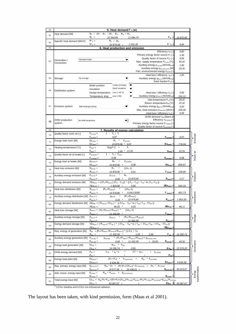
The layout has been taken, with kind permission, form (Maas et al 2001).
23
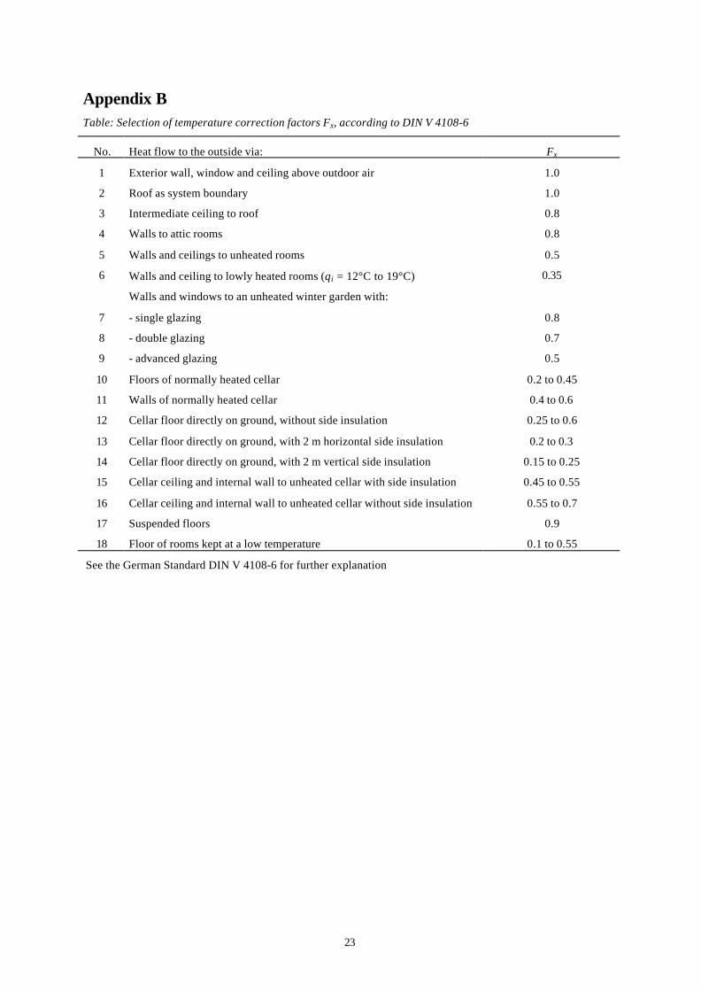
Appendix BTable: Selection of temperature correction factors Fx, according to DIN V 4108-6
No. Heat flow to the outside via: Fx
1 Exterior wall, window and ceiling above outdoor air 1.0
2 Roof as system boundary 1.0
3 Intermediate ceiling to roof 0.8
4 Walls to attic rooms 0.8
5 Walls and ceilings to unheated rooms 0.5
6 Walls and ceiling to lowly heated rooms (θi = 12°C to 19°C) 0.35
Walls and windows to an unheated winter garden with:
7 - single glazing 0.8
8 - double glazing 0.7
9 - advanced glazing 0.5
10 Floors of normally heated cellar 0.2 to 0.45
11 Walls of normally heated cellar 0.4 to 0.6
12 Cellar floor directly on ground, without side insulation 0.25 to 0.6
13 Cellar floor directly on ground, with 2 m horizontal side insulation 0.2 to 0.3
14 Cellar floor directly on ground, with 2 m vertical side insulation 0.15 to 0.25
15 Cellar ceiling and internal wall to unheated cellar with side insulation 0.45 to 0.55
16 Cellar ceiling and internal wall to unheated cellar without side insulation 0.55 to 0.7
17 Suspended floors 0.9
18 Floor of rooms kept at a low temperature 0.1 to 0.55
See the German Standard DIN V 4108-6 for further explanation
24
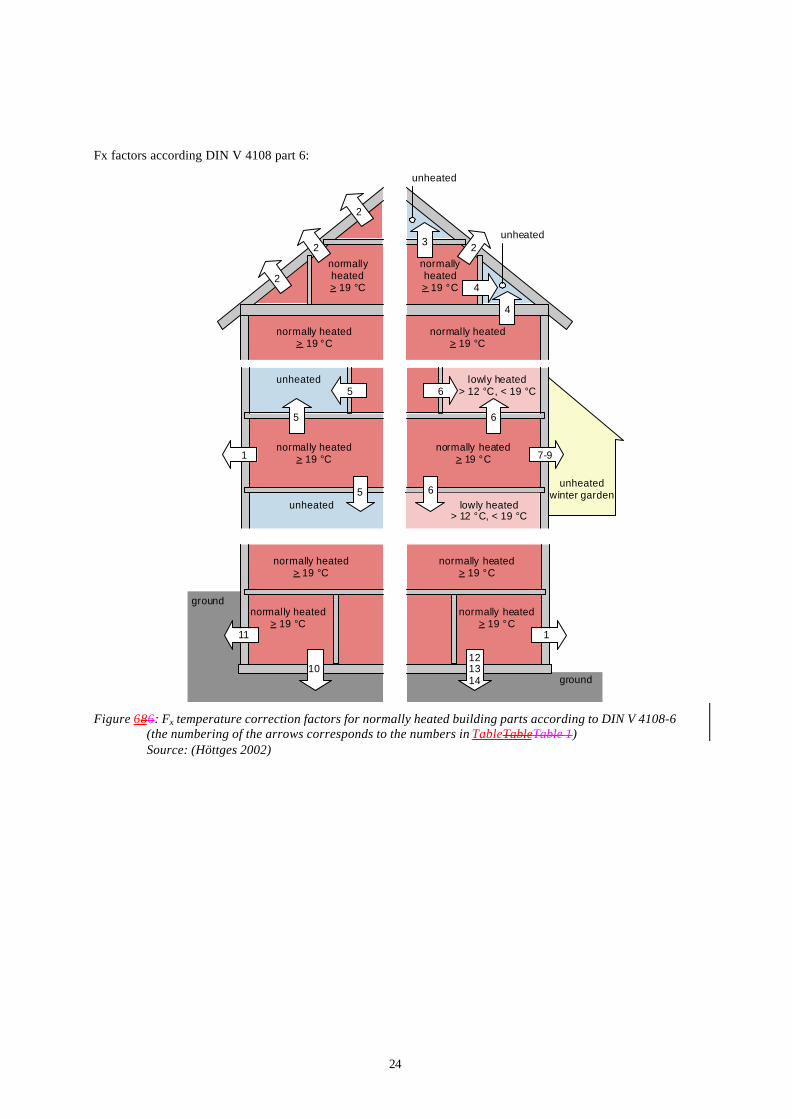
Fx factors according DIN V 4108 part 6:
normallyheated> 19 °C
normally heated> 19 °C
normallyheated> 19 °C
normally heated> 19 °C
unheated
2
2
2 3
4
4
2
unheated
normally heated> 19 °C
unheated
normally heated> 19 °C
unheatedwinter garden
unheated
lowly heated> 12 °C, < 19 °C
lowly heated> 12 °C, < 19 °C
1
5
5
5 6
6
7-9
6
normally heated> 19 °C
ground
ground
normally heated> 19 °C
normally heated> 19 °C
normally heated> 19 °C
11 1
121314
10
Figure 686: Fx temperature correction factors for normally heated building parts according to DIN V 4108-6(the numbering of the arrows corresponds to the numbers in TableTableTable 1)Source: (Höttges 2002)
25
lowly heated> 12 °C, < 19 °C
lowly heated> 12 °C, < 19 °C
lowly heated> 12 °C,< 19 °C
2
2
2 3
4
4
2
lowly heated> 12 °C,< 19 °C
unheated
unheated
lowly heated> 12 °C, < 19 °C
lowly heated> 12 °C, < 19 °C
lowly heated> 12 °C, < 19 °C
lowly heated> 12 °C, < 19 °C1
5
5
5
7-9
unheatedwinter garden
unheated
unheated
ground
ground
lowly heated> 12 °C, < 19 °C
lowly heated> 12 °C, < 19 °C
lowly heated> 12 °C, < 19 °C
lowly heated> 12 °C, < 19 °C
11 1
1810
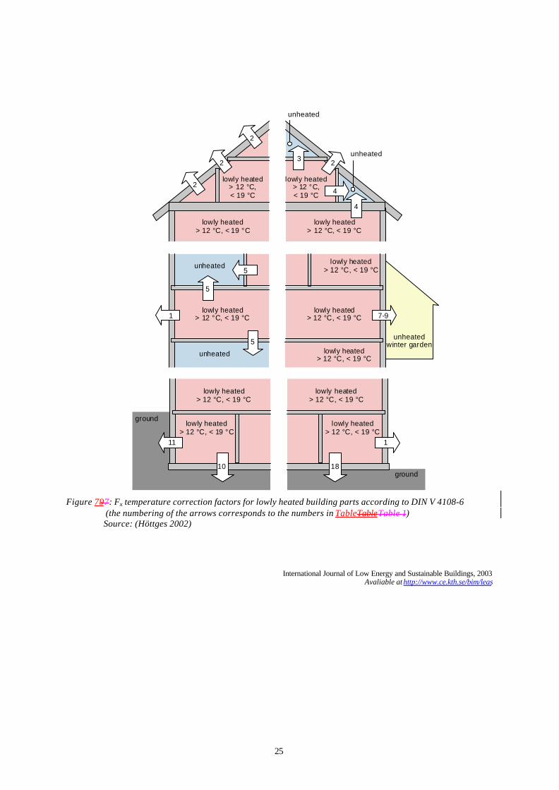
Figure 797: Fx temperature correction factors for lowly heated building parts according to DIN V 4108-6 (the numbering of the arrows corresponds to the numbers in TableTableTable 1)Source: (Höttges 2002)
International Journal of Low Energy and Sustainable Buildings, 2003Avaliable at http://www.ce.kth.se/bim/leas
26
Appendix CEquations, data and considerations used in the tool in the relevant sections
Equations used for the calculation of the heat demand
Transmission heat loss ΦT
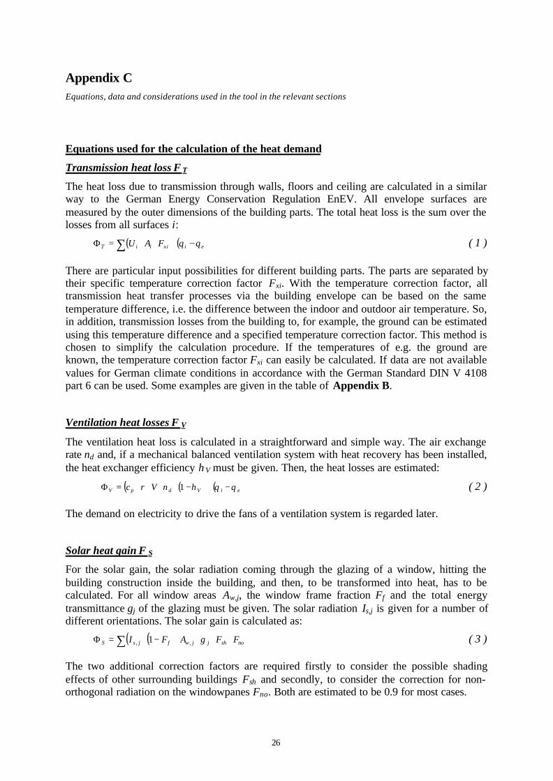
The heat loss due to transmission through walls, floors and ceiling are calculated in a similarway to the German Energy Conservation Regulation EnEV. All envelope surfaces aremeasured by the outer dimensions of the building parts. The total heat loss is the sum over thelosses from all surfaces i:
( ) ( )∑ −⋅⋅⋅=Φ eixiiiT FAU θθ ( 1 )
There are particular input possibilities for different building parts. The parts are separated bytheir specific temperature correction factor Fxi. With the temperature correction factor, alltransmission heat transfer processes via the building envelope can be based on the sametemperature difference, i.e. the difference between the indoor and outdoor air temperature. So,in addition, transmission losses from the building to, for example, the ground can be estimatedusing this temperature difference and a specified temperature correction factor. This method ischosen to simplify the calculation procedure. If the temperatures of e.g. the ground areknown, the temperature correction factor Fxi can easily be calculated. If data are not availablevalues for German climate conditions in accordance with the German Standard DIN V 4108part 6 can be used. Some examples are given in the table of Appendix B.
Ventilation heat losses Φ V
The ventilation heat loss is calculated in a straightforward and simple way. The air exchangerate nd and, if a mechanical balanced ventilation system with heat recovery has been installed,the heat exchanger efficiency ηV must be given. Then, the heat losses are estimated:
( )( ) ( )eiVdpV nVc θθηρ −⋅−⋅⋅⋅⋅=Φ 1 ( 2 )
The demand on electricity to drive the fans of a ventilation system is regarded later.
Solar heat gain Φ S
For the solar gain, the solar radiation coming through the glazing of a window, hitting thebuilding construction inside the building, and then, to be transformed into heat, has to becalculated. For all window areas Aw,j, the window frame fraction Ff and the total energytransmittance gj of the glazing must be given. The solar radiation Is,j is given for a number ofdifferent orientations. The solar gain is calculated as:
( )( )∑ ⋅⋅⋅⋅−⋅=Φ noshjjwfjsS FFgAFI ,, 1 ( 3 )
The two additional correction factors are required firstly to consider the possible shadingeffects of other surrounding buildings Fsh and secondly, to consider the correction for non-orthogonal radiation on the windowpanes Fno. Both are estimated to be 0.9 for most cases.

27
28
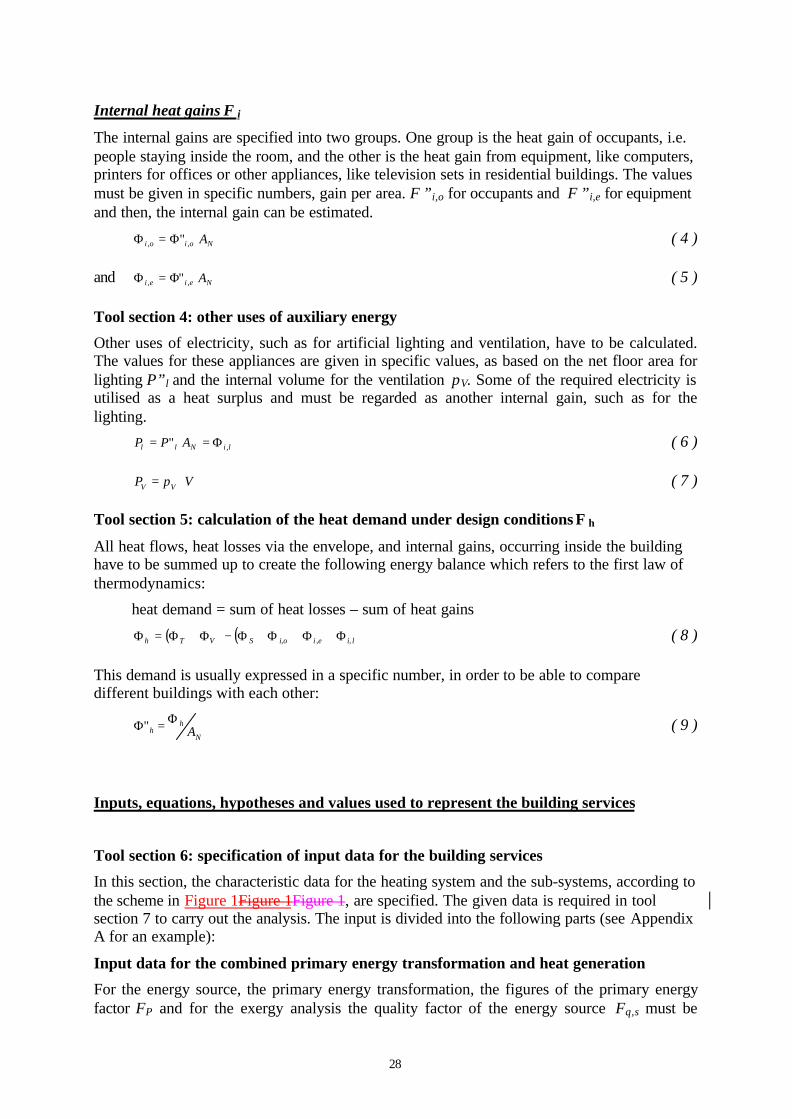
Internal heat gains Φ i
The internal gains are specified into two groups. One group is the heat gain of occupants, i.e.people staying inside the room, and the other is the heat gain from equipment, like computers,printers for offices or other appliances, like television sets in residential buildings. The valuesmust be given in specific numbers, gain per area. Φ”i,o for occupants and Φ”i,e for equipmentand then, the internal gain can be estimated.
Noioi A⋅Φ=Φ ,, " ( 4 )
and Neiei A⋅Φ=Φ ,, " ( 5 )
Tool section 4: other uses of auxiliary energy
Other uses of electricity, such as for artificial lighting and ventilation, have to be calculated.The values for these appliances are given in specific values, as based on the net floor area forlighting P”l and the internal volume for the ventilation pV. Some of the required electricity isutilised as a heat surplus and must be regarded as another internal gain, such as for thelighting.
liNll APP ," Φ=⋅= ( 6 )
VpP VV ⋅= ( 7 )
Tool section 5: calculation of the heat demand under design conditions Φh
All heat flows, heat losses via the envelope, and internal gains, occurring inside the buildinghave to be summed up to create the following energy balance which refers to the first law ofthermodynamics:
heat demand = sum of heat losses – sum of heat gains
( ) ( )lieioiSVTh ,,, Φ+Φ+Φ+Φ−Φ+Φ=Φ ( 8 )
This demand is usually expressed in a specific number, in order to be able to comparedifferent buildings with each other:
N
hh A
Φ=Φ" ( 9 )
Inputs, equations, hypotheses and values used to represent the building services
Tool section 6: specification of input data for the building services
In this section, the characteristic data for the heating system and the sub-systems, according tothe scheme in Figure 1Figure 1Figure 1, are specified. The given data is required in toolsection 7 to carry out the analysis. The input is divided into the following parts (see AppendixA for an example):
Input data for the combined primary energy transformation and heat generation
For the energy source, the primary energy transformation, the figures of the primary energyfactor FP and for the exergy analysis the quality factor of the energy source Fq,s must be

29
given. To divide the fossil part from the renewable part of the required primary energy, afraction factor for the environmental energy Frenew must be given.
Table 112: Characteristic data for energy/ exergy sources for the energy transformation. Source: DIN V 4701-10 1), Jóhannessson 20012) and Zirngibl Francois 2002 3)
Energy carrier Primary energyfactor FP
Quality factor Fq,s 2)
Fuel oil 1.1 1) 0.9
Natural gas 1.1 1) 0.9
Liquefied natural gas 1.1 1) 0.9
Mineral coal 1.1 1) 0.9
Brown coal 1.2 1) 0.9
Fuel (reference: net caloric value)
Wooden pellets 0.2 1) 0.8
Fossil fuel 0.7 1) 0.21District heating from combined heatand power plant at 100°C
Renewable fuel 0.0 1) 0.21
Fossil fuel 1.3 1) 0.21District heating from heat plant at100°C
Renewable fuel 0.1 1) 0.21
Electricity German mixture 3.0 1) 1.0
Electricity French mixture 2.58 3) 1.0
Electricity (estimate) Norwegian mixture 0.54 1.0
For the generation part, the boiler, the efficiency of the component ηG is the key figure.Auxiliary energy used in the generation, like electricity used to drive pumps, is regarded as afraction of the produced heat. This is given by an auxiliary energy factor paux,G. The typicalmaximum supply temperature of the boiler θS,max is needed to check the consistency of theoverall system design.
Table 223: Characteristic values for heat generation systems / boilers
Boiler type Thermal efficiencyηG (%)
Auxiliary powerpaux,G (W/kW)
Max. supply temperatureθS,max (°C)
LNG condensing boiler 0.99 0.02 60
LNG high temperature boiler 0.80 0.01 90
Electric boiler 0.98 0.01 90
District heating 0.99 0.01 100
The thermal efficiency of heat pumps must be regarded in a different way. Because of thespecific working principle of heat pumps, a coefficient of performance (COP), instead of athermal efficiency, is given to characterise this component. These COPs are not fixed. Theyvary with the working conditions, namely the supply temperatures to the distribution andemission system, of the heat pumps. In the tool, the COP is calculated for every system set-updependent upon the supply temperatures. The linear regression algorithm procedure is basedon values from the following table:Table 334: Minimum values for the performance coefficient of heat pumps in nominal conditions, COP.
Heat pump type water-borne heating system Air heating

30
at mid-temperature(θdis = 50 °C)
At low temperature(θdis = 35 °C)
External air/water 2.5 3.2
Exhaust air/incoming air 2.5
External air/recycled air 2.5
Exhaust air/water 2.2 2.7
Water/water 3.0 4.1
Water with glycol/water 2.4 3.0
Water/recycled air 3.0
Source: (Zirngibl and François 2002)
Note: The tool is not actually an energy performance calculation tool. The efficienciesassociated to generators are nominal values and don’t depend on the energy load of thebuilding.
Thermal losses are not put in relation with the nominal power of generators in order tocalculate the load. The user could take values corresponding to part load (intermediate loadof 30 %) instead of the full load.
Note: Combined Heat and Power generation - electricity production represents about half ofthe heat demand.
To assess this type of generator, one could take off the electricity production from theelectrical needs, even if the production occurs not at the same time as the needs (mean valuesare considered); if more electricity is produced than used, it could be valorised with theprimary energy factor of the electricity network.
Input data for the heat storage system
The heat storage system is characterised in round terms by specific heat loss or thermalefficiency ηS and by possible used auxiliary energy needed to run the storage, like electricityneeded to drive pumps. This is regarded as a fraction of the stored heat and given by anauxiliary energy factor paux,S.
In the tool, small day storage systems and seasonal storage systems are regarded separately.The values are summarised in Table below.
The heat loss of small size storage is estimated by using a cool down coefficient Cr as follows:
( ) tCVQ ambsrSSloss ⋅−⋅⋅= ϑϑ, ( 10 )
According to ( Zirngibl and François 2002) a typical value for the cool down coefficient is 4.2VS
-0.45 in Wh/l.K.day. For a typical storage situation in a single-family house, with 100 lstorage volume, a storage temperature of 60 °C and a ambient temperature around the storageof 15 °C results in:
( ) ( ) WhCCKlWhllSloss 1.9924/1560100.2.4100 45.0
, =°−°⋅⋅⋅=Φ − ( 11 )
In the case of a typical heating load for a case such as 1.8 kW, the thermal efficiency ηS is:
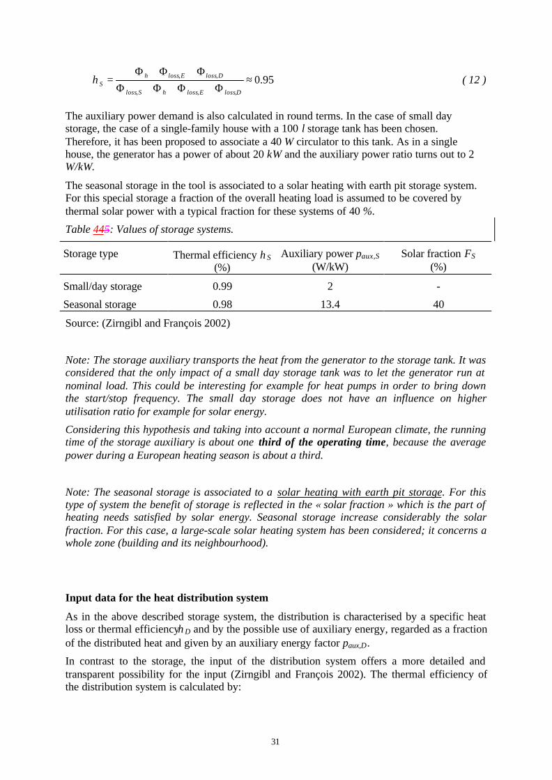
31
95.0,,,
,, ≈Φ+Φ+Φ+Φ
Φ+Φ+Φ=
DlossElosshSloss
DlossElosshSη ( 12 )
The auxiliary power demand is also calculated in round terms. In the case of small daystorage, the case of a single-family house with a 100 l storage tank has been chosen.Therefore, it has been proposed to associate a 40 W circulator to this tank. As in a singlehouse, the generator has a power of about 20 kW and the auxiliary power ratio turns out to 2W/kW.
The seasonal storage in the tool is associated to a solar heating with earth pit storage system.For this special storage a fraction of the overall heating load is assumed to be covered bythermal solar power with a typical fraction for these systems of 40 %.
Table 445: Values of storage systems.
Storage type Thermal efficiency ηS(%)
Auxiliary power paux,S
(W/kW)Solar fraction FS
(%)
Small/day storage 0.99 2 -
Seasonal storage 0.98 13.4 40
Source: (Zirngibl and François 2002)
Note: The storage auxiliary transports the heat from the generator to the storage tank. It wasconsidered that the only impact of a small day storage tank was to let the generator run atnominal load. This could be interesting for example for heat pumps in order to bring downthe start/stop frequency. The small day storage does not have an influence on higherutilisation ratio for example for solar energy.
Considering this hypothesis and taking into account a normal European climate, the runningtime of the storage auxiliary is about one third of the operating time, because the averagepower during a European heating season is about a third.
Note: The seasonal storage is associated to a solar heating with earth pit storage. For thistype of system the benefit of storage is reflected in the « solar fraction » which is the part ofheating needs satisfied by solar energy. Seasonal storage increase considerably the solarfraction. For this case, a large-scale solar heating system has been considered; it concerns awhole zone (building and its neighbourhood).
Input data for the heat distribution system
As in the above described storage system, the distribution is characterised by a specific heatloss or thermal efficiencyηD and by the possible use of auxiliary energy, regarded as a fractionof the distributed heat and given by an auxiliary energy factor paux,D.
In contrast to the storage, the input of the distribution system offers a more detailed andtransparent possibility for the input (Zirngibl and François 2002). The thermal efficiency ofthe distribution system is calculated by:
32
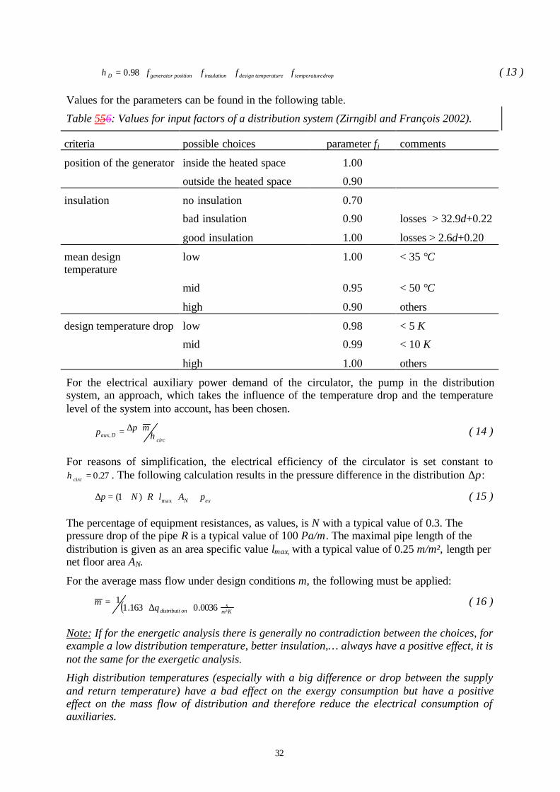
dropetemperaturetemperaturdesigninsulationpositiongeneratorD ffff ⋅⋅⋅⋅= 98.0η ( 13 )
Values for the parameters can be found in the following table.
Table 556: Values for input factors of a distribution system (Zirngibl and François 2002).
criteria possible choices parameter fi comments
position of the generator inside the heated space 1.00
outside the heated space 0.90
insulation no insulation 0.70
bad insulation 0.90 losses > 32.9d+0.22
good insulation 1.00 losses > 2.6d+0.20
mean designtemperature
low 1.00 < 35 °C
mid 0.95 < 50 °C
high 0.90 others
design temperature drop low 0.98 < 5 K
mid 0.99 < 10 K
high 1.00 others
For the electrical auxiliary power demand of the circulator, the pump in the distributionsystem, an approach, which takes the influence of the temperature drop and the temperaturelevel of the system into account, has been chosen.
circDaux
mpp η⋅∆=, ( 14 )
For reasons of simplification, the electrical efficiency of the circulator is set constant to27.0=circη . The following calculation results in the pressure difference in the distribution ∆p:
exN pAlRNp +⋅⋅⋅+=∆ max)1( ( 15 )
The percentage of equipment resistances, as values, is N with a typical value of 0.3. Thepressure drop of the pipe R is a typical value of 100 Pa/m. The maximal pipe length of thedistribution is given as an area specific value lmax, with a typical value of 0.25 m/m², length pernet floor area AN.
For the average mass flow under design conditions m, the following must be applied:
( )Kms
ondistributim
³0036.0163.11
⋅∆⋅= θ ( 16 )
Note: If for the energetic analysis there is generally no contradiction between the choices, forexample a low distribution temperature, better insulation,… always have a positive effect, it isnot the same for the exergetic analysis.
High distribution temperatures (especially with a big difference or drop between the supplyand return temperature) have a bad effect on the exergy consumption but have a positiveeffect on the mass flow of distribution and therefore reduce the electrical consumption ofauxiliaries.
33
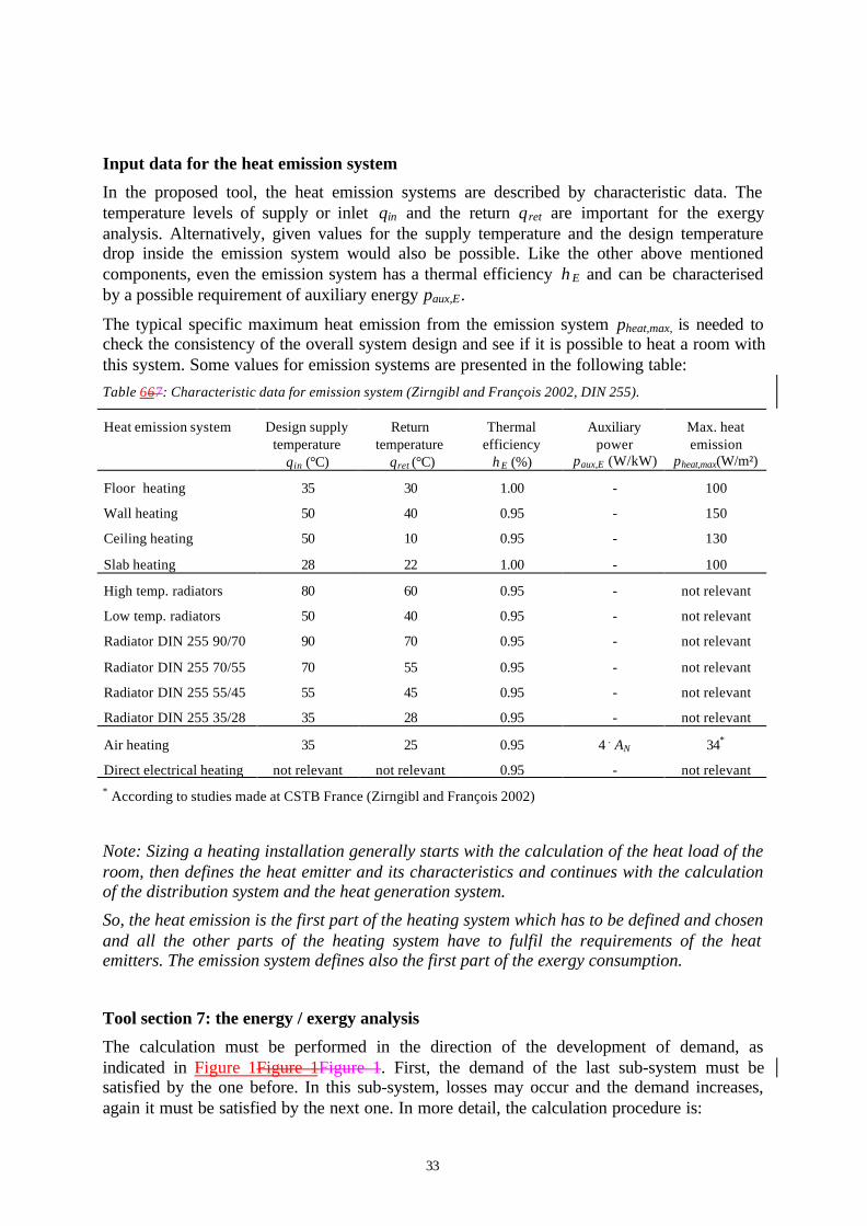
Input data for the heat emission system
In the proposed tool, the heat emission systems are described by characteristic data. Thetemperature levels of supply or inlet θin and the return θret are important for the exergyanalysis. Alternatively, given values for the supply temperature and the design temperaturedrop inside the emission system would also be possible. Like the other above mentionedcomponents, even the emission system has a thermal efficiency ηE and can be characterisedby a possible requirement of auxiliary energy paux,E.
The typical specific maximum heat emission from the emission system pheat,max, is needed tocheck the consistency of the overall system design and see if it is possible to heat a room withthis system. Some values for emission systems are presented in the following table:Table 667: Characteristic data for emission system (Zirngibl and François 2002, DIN 255).
Heat emission system Design supplytemperature
θin (°C)
Returntemperature
θret (°C)
Thermalefficiency
ηE (%)
Auxiliarypower
paux,E (W/kW)
Max. heatemission
pheat,max(W/m²)
Floor heating 35 30 1.00 - 100
Wall heating 50 40 0.95 - 150
Ceiling heating 50 10 0.95 - 130
Slab heating 28 22 1.00 - 100
High temp. radiators 80 60 0.95 - not relevant
Low temp. radiators 50 40 0.95 - not relevant
Radiator DIN 255 90/70 90 70 0.95 - not relevant
Radiator DIN 255 70/55 70 55 0.95 - not relevant
Radiator DIN 255 55/45 55 45 0.95 - not relevant
Radiator DIN 255 35/28 35 28 0.95 - not relevant
Air heating 35 25 0.95 4 . AN 34*
Direct electrical heating not relevant not relevant 0.95 - not relevant* According to studies made at CSTB France (Zirngibl and François 2002)
Note: Sizing a heating installation generally starts with the calculation of the heat load of theroom, then defines the heat emitter and its characteristics and continues with the calculationof the distribution system and the heat generation system.
So, the heat emission is the first part of the heating system which has to be defined and chosenand all the other parts of the heating system have to fulfil the requirements of the heatemitters. The emission system defines also the first part of the exergy consumption.
Tool section 7: the energy / exergy analysis
The calculation must be performed in the direction of the development of demand, asindicated in Figure 1Figure 1Figure 1. First, the demand of the last sub-system must besatisfied by the one before. In this sub-system, losses may occur and the demand increases,again it must be satisfied by the next one. In more detail, the calculation procedure is:

34
Energy / exergy calculations and analyses
Envelope sub-system, no. 7
The key figure for the first calculated step is the building’s heat demand Φh, calculated in theenergy balance equation. The quality factor of the room air Fq,room is estimated by means ofthe Carnot efficiency:
iroomq T
TF 0
, 1 −= ( 17 )
Then, the exergy load, i.e. the exergy demand of the room to be satisfied by the followingsub-system, is:
hroomqroom FEx Φ⋅= , ( 18 )
Room air sub-system, no. 6
The room is heated by a warm surface. The temperatures of the warm surface and of the roomalso give the exergy content at the heater surface and of the room. The temperature of theroom θi is modelled as one node. Effects of different surface and air temperatures, of radiativeand convective heat transfer processes between those, are neglected here. The surfacetemperature of the heater is estimated utilising the logarithmic mean temperature of the carriermedium with the inlet- and return temperature of the emission system (Moran and Shapiro1998):
i
iret
iin
retinheat θ
θθθθ
θθθ +⋅
−−
−= 2
1
ln
( 19 )
KT heatheat 15.273+= θ ( 20 )
Using this temperature, a new quality factor at the heater surface, can once again becalculated:
heatheatq T
TF 0
, 1 −= ( 21 )
The exergy load at the heater is:
hheatqheat FEx Φ⋅= ,
( 22)
Emission sub-system, no. 5
Because the energy efficiency of the emission system is not 100 %, an energy load calculationfirst has to be performed and the heat losses have to be calculated:
−⋅Φ=Φ 11
,E
hEloss η( 23 )
The demand on auxiliary energy or electricity of the emission system is:

35
hEauxEaux pP Φ⋅= ,, ( 24 )
Keeping the derivation of the exergy demand of the emission system in mind, it turns out that:
( )( ) ( )
⋅−−
−Φ+Φ
=∆ret
inoretin
retin
Elosshemis T
TTTT
TTEx ln, ( 25 )
The exergy load of the emission system is:
emisheatemis ExExEx ∆+= ( 26 )
Distribution sub-system, no. 4
For the distribution system a type of the calculation, similar to that used for the emissionsystem, is chosen. The heat loss of the distribution system is:
( )
−⋅Φ+Φ=Φ 11
,,D
ElosshDloss η( 27 )
The demand on auxiliary energy or electricity of the distribution system is:
( )ElosshDauxDaux pP ,,, Φ+Φ⋅= ( 28 )
The derivation of the exergy demand of the emission system is utilised. But the inlettemperature of the distribution system is the mean design temperature Tdis and the returntemperature is the design temperature minus the temperature drop ∆Tdis (note: used here asabsolute temperatures in K):
∆−
⋅−∆∆
Φ=∆
disdis
disodis
dis
Dlossdis TT
TTT
TEx ln, ( 29 )
The exergy load of the distribution system is:
disemisdis ExExEx ∆+= ( 30 )
Storage sub-system, no. 3
Again, the calculations chosen are similar to those used for the emission system. The heatlosses of the storage system are:
( )
−⋅Φ+Φ+Φ=Φ 11
,,,S
DlossElosshSloss η( 31 )
The demand on auxiliary energy or electricity of the storage system is:
( )DlossElosshSauxSaux pP ,,,, Φ+Φ+Φ⋅= ( 32 )
The derivation of the exergy demand of the emission system is once again utilised. But theinlet temperature of the storage system is the mean design temperature Tsto = Tdis + ∆Tdis , thereturn temperature is the design temperature minus the temperature drop ∆Tsto (note: used hereas absolute temperatures in K):

36
∆−∆+
∆+⋅−∆
∆Φ
=∆stodisdis
disdisosto
sto
Slosssto TTT
TTTT
TEx ln, ( 33 )
The exergy load of the storage system is:
stodissto ExExEx ∆+= ( 34 )
Generation sub-system, no. 2
The generation sub-system has to satisfy the demands of all previous sub-systems. If aseasonal storage is integrated into the system design, some of the required heat is covered bythermal solar power with a certain solar fraction FS. The required energy to be covered fromthe generator is:
( ) ( )G
SSlossDlossElosshGe F η11,,, ⋅−⋅Φ+Φ+Φ+Φ=Φ ( 35 )
The demand on auxiliary energy of the generation system to drive pumps and fans is:
( )SlossDlossElosshGauxGaux pP ,,,,, Φ+Φ+Φ+Φ⋅= ( 36 )
Since the generation system is supplied with an energy carrier, the exergy load of thegeneration is calculated directly:
SqGeGe FEx ,⋅Φ= ( 37 )
As a second step the exergy load of other building service appliances, such as lighting andventilation, are taken into consideration and here named “plant”.
( ) yelectricitqVlplant FPPEx ,⋅+= ( 38 )
Primary energy transformation sub-system, no. 1
The overall energy and exergy loads of the building are expressed in the required primaryenergy and exergy inputs. For the fossil or non-renewable part of the primary energy, theresult is:
yelectricitpEauxDauxSauxGauxVlPGetotprim FPPPPPPFE ,,,,,, )( ⋅++++++⋅Φ= ( 39 )
If the generation utilises a renewable energy source or extracts heat from the environment, asheat pumps do, the additional renewable energy load is:
environemtrenewGerenew EFE +⋅Φ= ( 40 )
The total exergy load of the building is:
renewqrenewSqtotprimtot FEFEEx ,,, ⋅+⋅= ( 41 )
This last figure is a key figure and can be used for a ranking in a specific value, for comparingbuildings and their efficiency and quality of exergy utilisation, and for evaluating the successof the exergy optimisation.

37
N
tottot A
ExEx ="