Educational Peer Effects

Quantile Regression Evidence from Denmark with

PISA2000 data

by

Beatrice Schindler Rangvid∗

∗AKF, Institute of Local Government Studies, Nyropsgade 37, DK-1602 Copenhagen V, Denmark.Phone: (45) 3311 0300, fax: (45) 3315 2875, and e-mail: bs@akf.dk.I thank Eskil Heinesen, Peter Jensen, Michael Rosholm, and participants at the ESPE2003 and

EALE2003 conferences and at AKF seminars for helpful comments and suggestions.

Abstract

We combine data from the first wave of the OECD PISA sample with register data for

Denmark to estimate educational peer effects. These datasets combined provide an un-

usually large set of background variables that help alleviate the usual problems of omitted

variables bias, prevalent in much of the empirical literature on peer effects. Quantile re-

gression results show that there may be differential peer group effects at different points

of the conditional test score distribution: The positive and significant peer level effect is

strongest for weak students and is steadily decreasing over the conditional test score dis-

tribution. The effect from a heterogenous peer composition on test scores does affect weak

learners positively, while the effect for good readers is negative, but at all estimated quan-

tiles, the effect is not significantly different from zero. These results combined suggest that

mixing of abilities is the optimal policy to maximize average reading skills in the student

population.

1 Introduction

Inputs in the process of accumulation of human capital operate at different levels. Some

are determined at the level of individual families, others at the level of the whole economy,

others again at the intermediate level of communities, neighborhoods, or social networks.

This is the case with many forms of ”social capital”, e.g. peer effects and role models.

Educational peer effects have long been of interest to social scientists because, if they

exist, they potentially affect the optimal organization of schools. The learning process at

schools depends crucially on how purchased inputs (teachers, buildings, books) combine

with social capital in the production of education. One expects peers to affect achievement

directly (e.g. helping each other with course work) and also via values (e.g. peers acting

as rolemodels).

The question is how best to educate students whose backgrounds and abilities differ

widely. However, the value of ability grouping in schools is a subject of much debate.

Proponents of ability grouping argue that by narrowing the range of student abilities

within a classroom, streaming allows teachers to target instruction at a level more closely

aligned with student needs than is possible in more heterogeneous environments, and that

student interest and participation are increased by ability grouping. On the other hand,

those opposed to ability grouping argue that less gifted students need the presence of their

higher level peers to stimulate learning, while average and even above average students

do not derive substantial academic benefits from being grouped together.

If the individual student’s scholastic achievement depends on the average quality of the

2

individual’s peer group, then, depending on the nature of the peer effects, there may be

social gains from grouping together ”high ability” students, or there could be social gains

from spreading high ability students evenly among the population. A welfare question

emerges: is it better to mix children’s qualities in schools, or should one educate them

in groups segregated by ability? Assuming that the social planner seeks to maximize

average academic achievement, the optimal policy turns on whether there are increasing

or decreasing returns to peer groups: with decreasing returns, one should mix children;

with increasing returns they should be segregated by ability. Thus, the optimal policy

becomes an empirical issue.

For governments to design policies that can improve socioeconomic outcomes, it is

critical that the educational production function and the relative importance of peer effects

versus other inputs such as teachers and infrastructure are better understood. It is clearly

difficult to think about improving student outcomes in schools until we know which inputs

matter. This study sheds some light on peer group effects in the Danish — non-selective —

school system.

The challenges of the Danish school system School systems around the world

differ in their extent of ability grouping of students during compulsory education. Some

countries have non-selective school systems (e.g. the Scandinavian countries) that seek

to provide all students with the same opportunities for learning. These countries limit

parental choice of school through fixed school catchment areas, there are no tracks or

streams, and automatic promotion regulates the transition from one grade to the next.

Other countries respond to diversity explicitly by forming groups of students of similar per-

formance levels through various mechanisms of the school system (e.g. Austria, Belgium,

Germany): tracking, streaming, grade retention, to name a few1, with the aim of serving

students according to their specific needs. And in yet other countries, combinations of the

two approaches occur.

While the issue whether or not to stream does not seem to be on the mind of many

European educational researchers or politicians, ability grouping has been an ongoing

debate in the United States for decades. Based on the research produced in the 1980s

on tracking, many schools and school systems have made major efforts to detrack. In

Denmark, a country with a completely non-selective school system, mixed-ability classes

and schools have been the corner stone of the compulsory school system. However, the

disappointing results for Denmark of the PISA (program for International Student As-

sessment) investigation conducted by the OECD (see OECD 2001a) in the year 2000 have

1Tracking usually means ability grouping of students either across schools or within schools for allsubjects, while streaming typically covers ability grouping within schools and for some subjects only. Thepractice of making students repeat a grade when his/her results are poor is called grade retention.

3

led to a fervent discussion on how to improve the academic achievement of Danish stu-

dents1. Compared to the other Scandinavian countries, Denmark produces relatively few

well-performing students and relatively many poorly performing students. As Danish ex-

penditure on education is among the highest among the OECD countries, any discussion

to yield achievement gains by raising general expenditures is ruled out2.

Denmark is a country with a completely non-selective school system with all students

taught in mixed-ability classes during compulsory schooling. There is almost no ability

grouping at all (only to a very small extent within the classroom), and there is almost

no chance for implicit ability grouping by choosing more or less advanced courses. The

only possibility for parents to choose a specific peer group for their child is at the school

level — either by residential location or by opting out of public school and choosing a

private school with a certain profile. However, even private schools are by no means

elitist in Denmark, but certain types of private schools attract certain types of students

(see Rangvid, 2003). For some years already, there has been an increasing awareness

of the pitfalls of a completely non-selective school system, and this criticism has led to

some within-class grouping. However, within-class grouping requires individual teachers

to manage several different groups of students simultaneously, thereby necessitating that

some groups of students spend considerable time working alone while the teacher is working

with other groups. Also, the PISA results show that Danish schools are comparably weak

at moderating the impact of socioeconomic disadvantage which might be due to the fact

that teaching has been targeted to the average student, while the weak and the strong

students have been left to themselves. For these groups, the parental background may

play a relatively stronger role than for the average student to whom teaching is targeted.

This discussion and the realization that a strong enough differentiation within the class

is not possible without the supply of many more resources in the form of teacher hours

has led to considerations whether to group students across grades by student ability at

least for some of the time. The suggestion has been to stream children during up to three

months of a school year, thus keeping the heterogenous classes intact for the remaining

time. This — rather cautious — suggestion for reform is due to the fact that ability grouping

is commonly viewed as increasing socioeconomic differences rather than moderating them.

By introducing limited and flexible regrouping schemes, the hope is to retrieve the benefits

from tailoring classes to each group’s ability, while maintaining the positive peer group

effects of a mixed-ability class.

1Actually, Denmark performed at the OECD average. However, for Denmark, the other Scandinaviancountries have traditionally been the relevant standard and Denmark underperformed compared to thesecountries.

2Also, Graversen and Heinesen (2002) provide evidence based on Danish data that the level of generalschool expenditure at best has a very limited effect on educational outcomes.

4

In any event, choosing the optimal degree of ability grouping is difficult; and the

optimal strategy is not only a matter of how and for how long to group students, but also

one of teacher attitude toward classes of varying abilities, curriculum issues like keeping

academic standards up also in low ability classes, etc.

Results from the literature The influence of peers on students’ achievement has

been a topic of extensive empirical and theoretical research. The peer group is undeniably

important in the minds of parents. Even in a mixed-ability school system, peer group

choice is exercised as residential location decisions of families have an implicit if not ex-

plicit peer group component (thus choosing between public schools). The role of peers

has entered increasingly into theoretical analyses of school choice3. But do peers have a

(measurable) impact on student performance? The findings in the existing literature on

peer effects are ambiguous. The standard approach to measuring peer effects regresses

students’ own outcomes on the peer ”quality” in the class or school (e.g. Summers and

Wolfe 1977; Henderson, Miezkowski, and Sauvageau, 1978; Betts and Morell, 1999; Zim-

mer and Toma, 2000). These studies on peer effects in a variety of countries all find

important educational peer effects4.

Generally, it is difficult to interpret coefficients obtained from this standard approach,

because individuals self-select into peer groups. This makes it difficult to distinguish the

selection effect from any actual peer effect. There are several approaches to dealing with

this sort of bias. Various authors attempt to solve the selection problem by designing

instruments for the peer group that are assumed to be exogenous. However, finding

credible instruments is difficult. Feinstein and Symons (1999) use local authority area

dummies to instrument for peer groups. The instrument is tested to be valid, but no

test of strength is reported. In a study of peer group effects on academic achievement,

Robertson and Symons (1996) employ regions of birth indicators to deal with the bias.

However, they do not present any formal or informal test of validity of the instruments.

In a recent study on another subsample of the PISA 2000 data we use in the present

study5, Fertig (2003) estimates the effect of a heterogenous classroom on reading skills,

3Starting from the observation that many people express concern about other students, a variety ofanalyses (e.g. Benabou 1993, 1996; Caucutt, 2001, forthcoming; de Bartolome, 1990; Epple and Romano,1998; Nechyba 1999, 2000) have examined how financing mechanisms, particularly vouchers, interact withdemands of families for different peers. Epple, Newlon, and Romano (2002) analyze the effects of abilitygrouping on school competition. Also in club theory, peer group effects have been incorporated. Standardclub theory shows that homogenous clubs are superior to mixed clubs on efficiency grounds (Berglas andPines 1981). Brueckner and Lee (1989) show in a variation on the standard club model that mixed clubscan be optimal when there are peer group effects.

4However, the size and significance of the peer effect for different groups of students differs acrossstudies.

5Fertig uses the US subsample, while we employ the Danish subsample of the international PISA 2000data.

5

using school selectivity, whether the school is a private school, and variables reflecting the

"caring behaviour" of parents as instruments. However, in spite of the fact that there

are multiple instruments, no test of overidentifying restrictions is offered to validate the

instruments.

In the closely related tracking literature, additional instruments for the peer group

have been suggested, e.g. regional indicators, urbanicity indicators and student body

characteristics (Argys, Rees and Brewer, 1996); two and three way interactions of three

variables: the number of academic courses required for state graduation, the number of

schools in the county, the fraction of voters in the county who voted for President Reagan

in the 1984 election (Figlio and Page, 2000); the percentage of black students in the school,

the percentage of students who receive full federal lunch assistance at the school, and the

students’ test score relative to the average for their grade (Betts and Shkolnik, 2000).

Some recent papers argue that estimating traditional ”average effect” models do not

give the full picture of the peer group effect, because they estimate the effect only for

the average student6. This may produce misleading results if peer group effects differ for

high and low ability students. By applying quantile regression techniques, it is possible to

give a more complete picture, because the peer effect can be estimated at all points of the

conditional test score distribution. Levin (2001) estimates peer group effects by quantile

regression techniques and finds that the number of similar classmates has the largest effect

on achievement of individuals at the lowest quantiles and that the peer effect experiences a

considerable monotonic decrease as one goes up the conditional achievement distribution,

and becomes insignificantly different from zero by the 90th percentile. Levin argues that

students at the lower end of the conditional achievement distribution are ”dependent”

learners relative to their higher achieving classmates for whom the effect of having similar

peers is negligible.

Despite of the attempts made in the literature, finding credible instruments seems to

be difficult7. Also, the results of the peer effect yielded in these studies are ambiguous.

Contribution In this study we provide evidence on the effect of ability grouping

by exploiting the degree of ability grouping across schools that is present in the existing

school system in Denmark: peer groups vary across schools due to geographical clustering

of families with different socioeconomic background and due to parental choice between

6However, several studies conduct subsample analyses of the peer effect.7This is especially true for observational cross section data. When panel data, natural experiments or

even true experimental data are available, there are additional possibilities, see e.g. Hanushek et al. , 2003;Lavy, 1999; and Goldhaber and Brewer, 1997 for panel data and Boozer and Cacciola, 2001; Sacerdote,2001; Zimmerman, 1999; and Hoxby (2000) for natural experiment; and Falk and Ichino (2003) for a trueexperiment in a different context.

6

the local public school and a range of private schools.

This is the first study on peer effects in Denmark, and one of the first studies on peer

effects to exploit the riches of the newly released PISA dataset8. The first wave of the

OECD PISA study provides a number of informative peer group variables as well as family

background variables. We use data from the first wave of the PISA study combined with

register-based data on the students’ backgrounds to estimate the effects of the level and

the variance of peer ability on the individual student’s educational achievement.

A crucial technical question we raise in this paper concerns the estimation of these

peer group effects by empirical methods. Due to the unavailability of suitable instruments

to account for self-selection into a peer group, we turn to a different strategy. The ability

to distinguish the separate effects of individual and school factors from those of peers

depends crucially on observing and measuring the inputs into students’ performance. The

typical analysis, however, does not have perfect measures of either family background or

school inputs. Thus, the endogeneity bias in our setting is basically an omitted variables

bias. Our strategy is to eliminate as much as possible of this bias by including variables

for parental characteristics that are typically thought to introduce the bias. While cer-

tainly not being "perfect" measures, yet, we have information available that permits us

to control for these effects, e.g. data on so-called parental academic interest, on home

educational resources, cultural interest, etc. (see section 2) — all variables which are un-

observed in ordinary datasets, but are thought to affect both parental choice of peers

and other (unobserved) parental input into the child’s schooling. Also, we estimate the

peer effect both for the average student and — using quantile regression techniques — at

different points of the conditional test score distribution to find out, whether high and low

performing students are affected differently by changes in the peer group. The effect of

class composition on academic achievement is explained via two main effects. The first is

the mean peer effect, namely externalities that are induced by the composition of teaching

and learning environment. The second is the efficiency effect, which reflects the reduced

ability of the teacher to teach and of the pupil to learn in a heterogenous environment.

We show that after controlling for a broad range of factors, there remains a statisti-

cally significant positive effect of the average of peer group quality with OLS estimation.

However, peer group heterogeneity does not seem to play an important role in Danish

classrooms, once the peer group level has been accounted for. Quantile regression evi-

dence reveals important differences of the peer effects at different parts of the conditional

8Two OECD (2001a, 2002) reports based on the dataset we employ in this study briefly address theissue of peer effect. The effect of the peer group is also briefly discussed in the Danish National PISAreport (2001). All studies find that peer group effects for Denmark exist, but the impact is far below theOECD average.

7

test score distribution. While the peer level effect is positive and significant at all esti-

mated quantiles, the point estimates are highest for weak readers and decrease steadily

over the conditional test score distribution. Also the peer heterogeneity effect is highest

at the lower quantiles, but unlike the peer average effect, it is imprecisely estimated for

all quantiles, and turns even negative (but is still insignificant) at the highest quantile.

The paper proceeds as follows. Section 2 presents the empirical framework. The

following section details the data. Section 4 reports results and sensitivity analyses, while

the last section concludes.

2 The empirical framework

To examine peer effects, we employ a standard education production function model.

These models estimate outcomes, e.g. test scores, as a function of the cumulative influence

of family and school inputs, the peers of the student, and individual characteristics of the

student. Conceptually, the model to be estimated is:

Aij = βXij + γSj + δPj + εij (1)

where Aij is achievement for student i at school j, Xij is a vector of individual and

family background influences, Sj is vector of school inputs, Pj is peer influence, and εij is

an error term.

If the student’s peer group is randomly assigned, or at least not systematically corre-

lated with unobserved factors influencing both the choice of the peer group and academic

achievement, then equation 1 provides us with an unbiased estimate of the peer group

effect, δ.

However, our concern is that the ”peer group” is often itself a matter of individual

choice, as is the implication of the classical Tiebout (1956) model of local finance. In a

Tiebout world, individual households, in making their locational choice, are also choosing

a peer group for many local services, including local public schools. In this setting, the

peer group becomes an endogenous variable, determined in part by household choice. Once

this is recognized, it is clear that models that do not correct for this kind of selectivity are

inappropriate. Thus, if students (or their parents) select into ability groups on the basis of

unobserved factors such as motivation or unobservable school quality, and if these factors

are, in turn, correlated with achievement, this approach will yield biased estimates of the

peer group effect. Formally, the error term in the selection equation may be correlated

with the error term of the achievement equation.

We suspect that simple models are likely to overstate peer group effects. Consider a

8

child with parents who do place a lot of importance on their child’s education. This child

will be a high-achiever in school for two reasons. First, the parents will choose a school

for their child with a positive learning environment, including a good peer group. Second,

the child will do better in school because the parents will encourage and back up their

child to reach a high academic level, i.e. parents who are exceptionally ambitious for their

children (in a manner unobserved by the econometrician) will choose high levels of the

productive inputs, e.g. the peer group, as well as aiding their child directly. If this type

of parental conduct is unobserved, empirical studies will tend mistakenly to allocate the

effect of the unobserved extra parental influence to the peer group.

There are several possible solutions to this problem. As discussed in the Introduction,

other authors have used such different approaches as instrumental variables methods,

panel data fixed effects estimators and quasi-experimental methods. However, due to

data limitations, (we do not have neither panel data, nor experimental data available for

our study) we cannot employ panel data techniques, neither do we have experimental

data. Moreover, according to our judgement, no study in the existing literature has come

up with convincing instruments.

Another strategy is to find a dataset which provides the researcher with data for the

relevant characteristics, which, when omitted due to data unavailability, introduce the

selectivity bias into single equation estimates. This is the strategy we will adopt in the

present paper: we shall deal with the bias, or at least reduce its effect, by including e.g.

data on parental academic interest and home educational resources — variables which are

unobserved in typical datasets, but are thought to affect both parental choice of peers and

other parental input into the child’s schooling.

We can do so, because basically, the selectivity problem is a problem of omitted vari-

ables. If we condition on all relevant variables, i.e. there were no unobservable character-

istics related to both the peer choice and the academic achievement equation, then single

equation models yield unbiased estimates. Thus, recall equation 1 and assume that the

vector of relevant family background variables9 can be decomposed into two parts: observ-

able characteristics, X1, such as gender, ethnicity, parental education, income, and family

structure, which are included in the typical empirical estimation in the literature; and un-

observable characteristics, X2, such as parental ambition, parental time spend with their

child, encouragement and support in their children’s education, etc., which are omitted

from the typical estimation in the literature, due to data unavailability.

9We suspect that in this setting the most important part of the bias is due to unobserved family charac-teristics — as the parents usually choose school for their child and at the same time parental characteristicsare the most important predictor of the child’s academic achievement.

9

Hence, the true model is

Aij = (β1X1ij + β2X2ij) + γSj + δPj + εij (2)

but the typical study estimates

Aij = β∗X1ij + γ∗Sj + δ∗Pj + νij (3)

where the error term now consists of unobservable family characteristics as well as a

random component (where νij = β02X2ij + εij). Thus by omitting X2ij , the estimation

of (3) may overstate the total effect of the peer group on academic achievement, because

omitted factors (X2ij) will not be included in the explained portion of the variance in

student achievement.

The obvious solution to this problem is to utilize data which include the relevant

variables in X2ij , or at least good proxies for them. In the present paper, the strategy is

to eliminate as much as possible of this bias by including variables for particularly parental

characteristics that are typically suspected of introducing the bias.

A main focus in the OECDs PISA study is the concept of family background influences.

Parental interest in the child’s education is regarded as one of the strongest predictors

for achievement in schools, and several questions in the student questionnaire aim to

tap information about the students’ home social background. In PISA, apart from the

usually collected variables on parental education, occupation, income and wealth, several

constructs related to family background variables that typically remain unobserved have

been derived from the student questionnaire. An important variable provided by the PISA

data is on parents’ support for their children’s education, which is widely recognized to be

an essential factor for success in school. When parents interact and communicate well with

their children, they can offer encouragement, demonstrate their interest in their children’s

progress, and otherwise show their concern for how their children are doing in school.

PISA divides parental involvement with their children into two indices: parental academic

interest and social communication. Parental academic interest is intended to measure

the level of academic and, more broadly, cultural competence in the student’s home.

Importantly, the construct also incorporates whether parents engage in these activities

together with their children. Social communication is designed to explicitly measure home

social capital, which means both parental involvement with their child in school matters

specifically, but also interest in the child’s life in general.

PISA also provides data on several other factors about the students’ home background

which are thought to be related to educational success. Student’s cultural activity focuses

10

on the student’s own cultural activities. Even though the construct clearly focuses on the

student’s own activities, there are strong reasons to believe that the tendency among 15-

year-olds to attend these kinds of activities is strongly linked to parental preferences and

practices. Home cultural possessions like classical literature, poetry and paintings have

frequently been shown to be related to educational success. Home educational resources

such as a desk for studying, textbooks, and computers focus on home resources that are

directly useful for the student’s schoolwork. These aspects of the home environment could

be said to indicate an academic orientation.

Thus, the PISA data give a wealth of information on the student parental background

that is usually unobserved by the econometrician, but is a potential source of the kind

of omitted variables bias described above. As will be shown, conditioning our estimates

on this extensive set of explanatory variables will produce estimates, where the bias is

significantly reduced.

Estimation methods We start by estimating peer effects by Ordinary Least Squares

(OLS), i.e. in an ”average causal effect” setting. We use sample weights as our sample is

stratified.

Most of the empirical work on peer effects focuses on average peer effects. However,

the standard methodology may miss how school resources affect achievement differently

at different points of the conditional test score distribution. For example, while the peer

group composition may not matter for average test scores, it would be useful to know

whether the true effect is zero at all points of the conditional test score distribution, or

whether the zero average effect covers up positive effects at some points of the distribution

and negative ones at others. This is especially relevant in the setting of peer composition,

if our analysis is to be relevant for policy advice: we must consider the best equilibrium

outcome, as giving a student a good peer is to take that peer away from someone else.

Thus, if weak readers profit from a better peer group, it is obvious that the best strategy

is mixing only if high-ability students are unaffected. With quantile regression, we are not

only able to address the question whether peer groups matter, but also for whom does the

peer group matter?

Over and above of allowing the researcher to focus on quantile treatment effects rather

than on average treatment effects, the quantile regression method has several other virtues.

First, the quantile regression estimator gives less weight to outlier data points on the de-

pendent variable than OLS, which weakens the impact such data points might have on

the results. In other words, every observation of the dependent variable can be made arbi-

trarily big or small without changing the results, as long as it does not cross the estimated

(hyper-) plane. Second, by allowing the parameter estimates for the marginal effects of the

11

explanatory variables to differ across the quantiles of the dependent variable, robustness

to potential heteroscedasticity is achieved. Third, when the error terms are non-normal,

quantile regression estimators may be more efficient than least squares estimators. The

main advantage, though, is the semi-parametric nature of the approach, which relaxes

the restrictions on the parameters to be constant across the entire distribution of the

dependent variables.

To appreciate quantile regression methods, it is worth emphasizing what quantile re-

gression is not about. Something like quantile regression cannot be achieved by dividing

the response variable into subsets according to its unconditional distribution and then do-

ing OLS on these subsets. This form of "truncation on the dependent variable" is clearly

not permissible. It is thus important to recognize that even for the extreme quantiles all

the sample observations are used in the process of quantile regression fitting.

The only paper we are aware of estimating peer group effects by quantile regression

methods is Levin (2001)10. However, in a slightly different context, Eide and Showalter

(1998) have used quantile regression techniques to estimate the effect of school resources

on test scores.

Originally, quantile regressions were suggested by Koenker and Basset (1978) as a

”robust” regression technique alternative to Ordinary Least Squares for the case when

the errors are not normally distributed. More recently, the quantile regression technique

has been applied not because of its robust property, but because of its feature to estimate

effects at different points of the conditional outcome distribution.

The basic quantile regression model specifies the conditional quantile as a linear func-

tion of covariates. For the θth quantile, a common way to write the model (see, e.g.

Buchinsky, 1998) is

yi= x0iβθ+uθi, Quantθ(yi|xi) = x0iβθ θ ∈ (0, 1) (4)

where Quantθ(yi|xi) denotes the quantile of yi, conditional on the regressor vector xi.The distribution of the error term is left unspecified. It is only assumed that uθi satisfies

the quantile restriction Quantθ(uθi|xi) = 0. The θth regression quantile (0 < θ < 1) of y

is the solution to the minimization of the sum of absolute deviations residuals

minβ

1

n

Xi:yi≥x0iβ

θ¯̄yi − x0iβ

¯̄+X

i:yi<x0iβ

(1− θ)¯̄yi − x0iβ

¯̄ (5)

The variation in the value of θ traces the entire distribution of test scores and one can

10However, several studies estimate peer effects on subgroup of students, where the sample is dividedinto subsets defined according to the independent variables.

12

estimate the peer effect on reading scores at any given percentile. The important feature

of this framework is that the marginal effects of the covariates, given by βθ, may differ

over quantiles (i.e., different values of θ). In the special case where yi = x0iβ + ui (with

ui homoscedastic), the marginal effects at every quantile will be the same11. Variation

in the estimated peer effects across the quantiles of the conditional distribution of read-

ing scores may be an indication of heterogenous peer effects. Therefore, we estimate an

education production function at different quantiles (θ = 0.1, 0.25, 0.5, 0.75, 0.9), and ex-

amine whether there is homogeneity in the effect of peers on individual reading literacy,

by testing for the equality of the peer effect coefficients across the quantiles.

Different quantiles are estimated by weighting the residuals differently. For the me-

dian regression, all residuals receive equal weight. However, when estimating the 75th

percentile, negative residuals are weighted by 0.25 and positive residuals by 0.75. The

criterion is minimized, when 75 percent of the residuals are negative. This is set up

as a linear programming problem and solved. Algorithms based on the least absolute

deviations criterion are available in order to obtain estimates.

While finding the solution to (5) is straightforward, the estimation of the variance-

covariance matrix is not. For the case of homoscedastic residuals, Koenker and Bassett

(1982) propose a formula. However, Rogers (1992) and Gould (1992) argue that, while this

method works adequately under the assumption of homoscedastic errors, it underestimates

the standard errors in the presence of heteroscedasticity, which is especially troublesome

as heteroscedasticity is often the reason for using quantile regression in the first place12.

It is therefore important to use some other method for estimating standard errors, such

as bootstrap re-sampling techniques. In the present study, standard errors are obtained

by bootstrapping the entire vector of observations. We use the design matrix bootstrap,

where pairs (xi,yi) i=1,...,n are drawn at random from the original observations with

replacement. For each of these samples drawn, an estimator of the parameters vector, βθis recomputed. Repeating this procedure B times yields a sample of B parameter vectors

whose sample covariance matrix constitutes a valid estimator of the covariance matrix

of the original estimator. This procedure is automated in the Stata statistical package.

However, the question of how to choose the number of bootstrap repetitions remains.

Andrews and Buchinsky (2000) suggest a three-step method to choose the number for

which they provide Monte Carlo simulations in Andrews and Buchinsky (2001). Their

findings are that the number of bootstrap repetitions commonly used in econometric

applications is much less than needed to achieve accurate bootstrap quantities. As the

11The slope coefficients on any variable will be the same across quantiles, though the intercept will differacross quantiles.12 In our paper, the analytically calculated standard errors were up to 25% smaller than the bootstrapped

errors.

13

sufficient number of bootstrap repetitions is inversely related to sample size, we chose the

number of 200 bootstrap repetitions.

If peer effects are homogenous across the conditional distribution, we would expect

the slope coefficients estimated at the quantiles to be equal. A method to formally test

the presence of heterogeneity in the peer effects is to test whether the observed differences

along the estimated coefficients are statistically significant across quantiles. Equality of

selected subsets of parameters between quantiles may be tested by estimating all quan-

tile equations simultaneously and thereby obtaining an estimate of the entire variance-

covariance matrix (including between-quantiles blocks) of the estimators by bootstrapping.

Thus, tests concerning coefficients across equations can be performed. For example, a test

of the hypothesis of heterogeneity (βθ 6= βδ for some θ) can be based on a test of whether

the estimated peer effect coefficients differ across quantiles.

3 Data

Sample We use data for Denmark from the OECD program for International Student

Assessment (PISA). The first PISA survey was conducted in the year 2000 in 32 countries.

PISA 2000 surveyed reading literacy, mathematical literacy and scientific literacy. In this

study, we use only reading test scores as our academic achievement measure13. The test

focusses on the demonstration of knowledge and skills in a form that is relevant to everyday

life challenges rather than how well students had mastered a specific school curriculum.

Students were tested in three "type of reading" tasks: retrieving information, interpreting

texts, and reflection and evaluation. To facilitate the interpretation of the scores assigned

to students, scores from these three tasks were summarized in a combined reading literacy

scale. This scale was designed to have an OECD average score of 500 points and a

standard deviation of 100 points. In Denmark, the test score distribution is rather tight

with a standard deviation of only 93 points compared to the OECD average of 100 points.

In addition to the reading literacy test, students answered a background questionnaire

and school principals completed a questionnaire about their school. In Denmark, the

sample is stratified by school size (very small, small and big schools). Within the strata,

schools were selected in a specific way so each student had an equal opportunity to be

selected irrespective of the size of the school or the class. Within each school, 28 students

aged 15 were selected randomly for participation14. For Denmark, the final PISA sample

consists of 223 participating schools with 4212 students corresponding to a responsrate of

13While the reading test was administered to every student participating in the assessment, the mathe-matics and the science tests were only given to one out of two students, thus rendering the mathematicsand science samples too small to obtain reliable estimates.14 In schools with less than 28 15-year-old students, all of them participated.

14

87 percent.

Register data As our identification approach is to minimize the amount of unobserved

characteristics which might influence both peer group choice and educational achievement,

we use Danish register data in addition to the PISA survey data, to complement the picture

of the family background available from the PISA data. Some variables are available both

from the survey and from registers.

The use of register data added information on parents’ income, type of housing,

whether the parents were "teens" when their child was born, a more complete measure

of parental education (e.g. detailing the length of tertiary education), and the amount

of parental unemployment in the year when the student was 15 years old. Other in-

formation, such as information on the family structure, is also available from the PISA

questionnaire, but can now be cross-checked with registerdata. In section 4, we conduct

selectivity analyses to check for disparities between survey and register variables.

We relied on several criteria to select the sample for our study from the larger PISA

sample. First, we restricted the sample to students attending schools for which PISA

provided data for at least 15 students. This restriction is necessary because for use in

the estimation, we construct peer measures from mean characteristics of the 15-year-old

students in a school, and we prefer to be sure of some minimum number of observations

for each school. The minimum number of 15 students might seem low, but was chosen as

not to lose too many observations from the sample.

We also include dummy variables to control for missing values of some explanatory

variables, in which case the explanatory variable was set to zero. E.g. in an important

number of cases, data on a parent’s occupational status were missing. Also, school back-

ground variables were missing in a significant number of cases, and we include dummy

variables for these missing observations as well. In spite of the introduction of missing

categories for some key variables, we lost 163 observations due to missing values in other

variables. Our final sample includes 3666 cases.

Peer quality and heterogeneity The peer variable is of primary importance in this

research. Building on the existing literature, we define the peer variable in terms of ability

and measure it in several ways. When we talk about peer ”quality”, we have in mind both

intellectual ability and other characteristics such as ambition, docility, punctuality and so

on, which we believe are derived in large part from the child’s home environment, and in

the schooling setting perhaps especially from the educational level of the parents. In our

basic estimations, we proxy peer quality by the average years of schooling of the classmates’

15

mothers15 16. We refrain from using the more obvious average level of reading scores of

the classmates as a proxy for class ability due to potential problems with reverse causality.

In this paper, we suggest that there are peer effects in the classroom. Consequently, if

each single student in the classroom is affected by his peers, the average achievement of

the classmates is affected by each single student, too — giving rise to reverse causality

problems.

As part of the sensitivity analysis reported in section 4, we also use additional measures

of peer quality.

We also square mean parental education to capture nonlinear as well as linear effects

of the average on fellow students. It is generally assumed in the literature that the higher

the mean score of fellow students in a class, the higher the level of educational attainment

of a given student, but the effect may diminish (i.e. the squared term is expected to be

negative.) Additional interaction variables to capture peer effects will be introduced in

variations on the basic empirical model.

In addition to these peer mean variables, we control for the heterogeneity of the peer

group, because if a better peer group in the data is correlated with a homogenous class-

room, then a potentially positive effect from a homogenous peer group will be falsely

attributed to a higher peer quality. The variance, or mix, of abilities within the classroom

may affect individual student achievement and we are interested in assessing the effect of

being schooled in a classroom with similarly skilled students relative to the effect of being

schooled in a classroom that has a larger variance in student abilities. For example, a

classroom in which all students have roughly the same ability may generate different peer

effects than one with the same mean score, but a wide range of abilities. Teachers of a

homogenous high ability class can provide them with more challenging material or present

standard material at a faster pace than would be possible in a classroom where less-able

students’ needs also have to be met. At the same time, low-ability students are expected

to benefit from the slower pace or alternative teaching methods that become feasible when

teachers are not simultaneously responsible for engaging the students’ high-ability peers.

To analyze this, we include the standard deviation of parental education of all students

in the classroom as a measure of classroom heterogeneity.

Our peer data is only approximately class peer data, as 15-year-old students were

selected randomly within schools, irrespective of the grade or class within grades. However,

15We have tried other specification as well: years of schooling of classmates’ fathers and average yearsof schooling of parents without a qualitative change in the results.16Behrman and Rosenzweig’s (2002) results suggest that the postive relationship between the schooling

of mothers and their children is substantially biased upward due to correlations between schooling andheritable "ability" as well as assortative mating. In other words: more able women, who have moreschooling, have more able children, who obtain more schooling; and: more schooled women marry moreschooled (and thus more able) men.

16

in a system like the Danish, where students are not grouped by ability across classes, the

peer composition of 15-year-olds within a school will be an acceptable proxy for the peer

composition within the classes, the 15-year-old students attend.

Control variables Other variables than the peer group are important for academic

achievement. Particularly parental inputs are commonly found to be immensely significant

in determining both choice of peer group and academic achievement, while the importance

of school level inputs is much more disputed in the literature. The control variables can

be divided into two main categories: home-related factors and school-related factors.

— Home-related inputs The model controls for the typically employed background

variables which are likely to affect test scores and/or peer group choice, e.g. age17,

gender, ethnicity, number of siblings, sibling status (only child; oldest, middle,

youngest child), family structure, parental education, parental occupation, parental

income, and parental wealth, and whether the student speaks Danish at home. In

addition to the background variables available in a typical dataset, the PISA dataset

provides us with variables, which are thought to be important for the parents’ influ-

ence on the child’s peer group and on his educational achievement. Such variables

are e.g. the index18 measuring parental academic interest, which was derived from

students’ reports on the frequency with which their parents engaged with them in

discussing political or social issues, discussing books, films or television programs,

and listen to classical music. The index for cultural possessions in a family’s home

was derived from students’ reports on the availability of classical literature, books

of poetry and works of art in the home, while the social communication index was

based on the frequency with which parents discussed how well their child is doing at

school, whether they eat the main meal with him around the table, and how often

they spend time simply talking with him. The index for home educational resources

was derived from students’ reports on the availability and number of dictionaries, a

quiet place to study, a desk for study, textbooks, and calculators. Students’ cultural

activity is an index on how often students had visited a museum or an art gallery dur-

ing the preceding year, attended an opera, ballet or classical symphony concert, and

watched live theatre. All these variables are proxies for parental interest in the child,

either directly in education matters, or general interest. They, also, indicate general

17Although the students were tested in the year were they turned 15, the oldest students (born in thebeginning of the year) will be almost a year older than the students born at the end of that year. We thusmeasure their age in months to take account of potential age effects.18Several summary indices were created for the official PISA dataset. They summarize students’ or

school principals’ responses to a series of related questions selected from larger constructs on the basis oftheoretical considerations and previous research. Indices were standardised so that the mean of the indexvalue for the OECD student population was zero and the standard deviation was one. See OECD (2001b)for details on the construction of the indices.

17

parental interest in culture and education. These are variables, which are thought

to be crucial for both the peer group choice parents directly or indirectly make for

their children, and at the same time do such factors proxy for how much, and how

qualified parental support the child will receive to promote academic achievement.

Moreover, information is available on time spent on homework for Danish lessons,

type of housing, and whether the parents were in their teens when their child was

born.

— School-related inputs Hanushek (2002) points out that "characterizing school qual-

ity has been difficult, and thus it is highly likely that standard estimation of educa-

tional production functions with peers will overstate peer influence". In the present

study we will therefore include various variables at the school and class level which

potentially influence achievement and school (peer) choice.

We expect students to benefit from teaching practices that demonstrate teachers’

interest in the progress of their students, when teachers expect their students to

attain reasonable achievement standards, and when they are willing to help all stu-

dents to meet these standards. The responses were combined to create an index of

teacher support. Also, teacher behaviour is of importance for the learning environ-

ment, such as whether learning is hindered by low expectations of teachers, poor

student-teacher relations, absenteeism among teachers, staff resistance to change,

teachers not meeting individual students’ needs, and students not being encouraged

to achieve their full potential. Factors related to teacher education are also gener-

ally considered important. We use PISA data on how many of the teachers teaching

Danish at the school are certified in Danish, and how many teachers have partici-

pated in professional development within the last three months.

In the empirical literature, the effect of school resources on scholastic achievement

has produced few significant results. Hanushek (1986, 1996) provides an extensive

discussion of this evidence. However, some recent studies have found more posi-

tive evidence (e.g. Card and Krueger 1992, Angrist and Lavy 1999, Krueger 1999,

Wilson 2002). To avoid any confounding influences from systematic variations of

school resources, we include class size as a measure of school resources in our esti-

mations. Also, the absence of a suitable physical infrastructure (e.g. buildings) and

an adequate supply of educational resources (computers, library, teaching materials)

might hinder learning. Two indices were created by the PISA consortium — one for

the perceived quality of the school’s physical infrastructure and the other for the

perceived quality of educational resources. Also, the number of Danish lessons per

week, the total number of teaching lessons per year and the frequency with which

students use school resources, like e.g. the library, are used as controls.

Private schools are sometimes perceived to be more effective in teaching children.

18

Especially in the Danish context, private schools have a great liberty with respect

to the choice of curriculum and teaching methods. On the other hand, in a non-

selective school system, private schools might be used as an alternative if the local

public school is of low (peer) quality. We control for the type of school to investigate

how the institutional arrangement of schools is related to student performance. Also,

school size might be related to student achievement, due, for example, to economies

of scale in the use of educational and economic resources.

There is a range of other student and school variables available in the PISA dataset,

e.g. whether students attend special courses to improve results. However, we suspect

there to be a large amount of reverse causality between reading skills and these variables,

which is the reason for their omission from the estimations.

Table 1 provides descriptive statistics of the dataset used for the estimations.

19

Table 1: Descriptive statisticsVariable description Mean Std.dev. Min MaxMain variables of interestPISA reading score 501.9 93.4 89.3 887.3Mean parental education of peers (years) 12.34 1.30 7.53 15.03Std.dev. of parental education of peers 3.83 1.02 2.00 6.83Background variablesGender (Male=0, Female=1) .50 .50 0 1Student’s age at test 15.72 .27 15.25 16.17Ethnic Dane .95 22 0 1Immigrant .03 .18 0 1Parents immigrated .02 .12 0 1Does not speak Danish at home .05 .22 0 1Number of brothers/sisters 1.90 1.28 0 12Student is only child .06 .23 0 1Student is oldest child .36 .48 0 1Student is middle child .23 .42 0 1Student is youngest child .35 .48 0 1Student lives in nuclear family .67 .47 0 1... lives with single mother .13 .34 0 1... lives with mother and stepdad .10 .29 0 1... lives with single dad .02 .15 0 1... lives with father and stepmum .02 .13 0 1... lives without parents .06 .23 0 1... lives without parents (but parents live together) .01 .09 0 1Student’s mother was teen at birth .09 .28 0 1Student’s father was teen at birth .10 .29 0 1Mother: unskilled .21 .41 0 1

- high-school degree .04 .20 0 1- vocational education .30 .46 0 1- short college .04 .20 0 1- long college .21 .41 0 1- university .03 .18 0 1- PhD .003 .05 0 1

Father unskilled .29 .45 0 1- high-school degree .03 .18 0 1- vocational education .41 .49 0 1- short college .04 .20 0 1- long college .11 .31 0 1- university .07 .26 0 1- PhD .003 .029 0 1

Mother: Legislator, senior official or manager .03 .17 0 1- Professional .11 .32 0 1- Technician or associate professional .19 .39 0 1- Clerk .15 .36 0 1- Service worker/shop&market sales worker .17 .37 0 1- Skilled agricultural or fishery worker .00 .07 0 1- Craft or related trades worker .02 .13 0 1

(...continued)

20

... continuedVariable description Mean Std.dev. Min Max

- Plant or machine operator or assembler .04 .20 0 1- Elementary occupations .14 .35 0 1- Armed forces <.00 .02 0 1

Father: Legislator, senior official or manager .08 .28 0 1- Professional .13 .33 0 1- Technician or associate professional .11 .32 0 1- Clerk .03 .17 0 1- Service worker/shop&market sales worker .04 .20 0 1- Skilled agricultural or fishery worker .04 .21 0 1- Craft or related trades worker .17 .37 0 1- Plant or machine operator or assembler .08 .27 0 1- Elementary occupations .10 .29 0 1- Armed forces .01 .08 0 1

Mother’s income .19 .10 0 2.08Father’s income .29 .21 0 3.12Mother’s unemployment at student’s age 15 .05 .16 0 1Father’s unemployment at student’s age 15 .03 .14 0 1Family wealth .53 .74 -3.00 3.38Parents home-owners .72 .45 0 1Parents home-renters .19 .39 0 1Parents living in not categorized type of dwelling .01 .12 0 1Parents’ type of dwelling unknown .07 .26 0 1Index of parental academic interest .11 .98 -2.2 2.72— missing .001 .03 0 1Index of social communication .22 .89 -3.65 1.2Index of cultural possessions -.11 .97 -1.65 1.15Index of cultural activity .28 .90 -1.28 2.93Student has quiet place to study .87 .33 0 1Index of home educational resources -.20 .92 -3.99 .76Class size in Danish lessons 17.63 3.52 1 28Class size in Danish lessons, missing .10 .30 0 1Number of Danish lessons/week 7.09 1.81 1 20Number of Danish lessons, miss. .31 .46 0 1Hours spent on homework in Danish 2.96 .71 1 4Data on homework (Danish) missing .014 .12 0 1Index of teacher support .12 .70 -3.03 1.95Index of teacher behaviour -.52 .77 -2.41 1.22School physical infrastructure .04 .73 -1.12 3.38School educational resources -.16 .63 -1.90 2.48Certified Danish teachers .41 .34 0 1Frequency of library use etc. .84 1.01 -2.46 4.43

... continued

21

... continuedVariable description Mean Std. Min MaxSchooling hours per year 881.83 153.48 594 1400Number of students at school 437.13 195.93 49 917Percentage of teachers on professional development .48 .31 .05 1School type (Public school=0, private=1) .12 .32 0 1Indicator: Variables at school level missing .33 .47 0 1

3666

Before going on to the estimations, let’s have a short look at raw correlations between

the variables of primary interest. In Table 2, we report results from simple OLS models

regressing reading scores on either the mean peer level of parental (mothers’) years of

schooling in each student’s classroom, the classroom heterogeneity or both. The results

show that the mean peer level (PeerMean) is positively correlated with reading scores,

and peer heterogeneity is negatively so (favouring homogenous classrooms, i.e. streaming

students), when they are entered separately.

Table 2: Simple models

Reading scores (1) (2) (3)

Coeff. Std.dev. Coeff. Std.dev. Coeff. Std.dev.

PeerMean 15.35 1.16 ∗∗∗ - 18.41 1.63 ∗∗∗

PeerHetero - -11.03 1.51 ∗∗∗ 5.57 2.09 ∗∗∗

Adj. R2 .045 .014 .047∗∗∗ indicates significance at the .001 level.

However, as we suspected earlier, peer level and peer heterogeneity are not uncorre-

lated. As can be seen from Figure 1, there is a clear tendency between the peer level

of a class and the heterogeneity of the class peers. Classes with a high peer level tend

to be more homogenous than classes with a lower peer level19. When we enter the peer

level and peer heterogeneity variable jointly in a regression (see Table 2, model (3)), the

coefficient on peer heterogeneity turns positive. So, the large negative correlation between

achievement and class-heterogeneity is clearly a result of the association between more

heterogenous classes and lower parental education among pupils20.

The following section presents results.

4 Results

To begin with, we will motivate our choice of variables for the main estimations. We then

report OLS results, followed by results from quantile regressions and discussion.

19 In the extremes of the joint distribution, this could be a mechanical relation, as high-level classes mustbe quite homogenous to reach a very high level of peer average. However, when we trim the sample, so wedrop the observations with the 5% highest peer mean level, results are basically unchanged.20This finding is confirmed by Lavy (1999) for schools in Israel.

22

PeerHetero

PeerMean7.53333 15.0263

2.00329

6.82891

Figure 1: Correlation between peer mean and peer variance

4.1 Choosing the set of controls

As pointed out earlier, the estimation strategy for isolating the causal effect of school peers

is to condition on a very broad set of factors that may affect both achievement and peer

composition. This approach implies "washing out" the problem of unobserved ability by

including a broad range of background variables in the regressions. Our data provides an

extensive set of control variables that help avoid the usual problems of omitted variables

bias. In addition to the standard set of controls (parental education, occupation, income

and wealth; family structure, siblings, ethnicity, bilingual, gender, class size, teacher qual-

ification = model (i) in Table 3), the PISA dataset provides us with other information on

factors thought to be important for both the choice of peers and for reading skills. These

variables are: parental academic interest, social communication, cultural possessions and

activity, whether the student has a quiet place for study at home, the amount of time

spend on homework and study for Danish lessons; and school resource variables like the

number of Danish lessons per week, teacher support, teacher behaviour, the quality of

the school building and the educational material in school, use of school resources, the

student-teacher relationship, total hours of teaching, school size, the share of teachers hav-

ing participated in extra qualification courses during the last three months, and whether

the school is public or private ( = model (ii) in Table 3).

We then add information from administrative registers on the parents’ occupation,

their housing conditions and whether they were teen-parents (model iii). Last, we ex-

change some survey variables with information from the registers, because they are more

detailed and also, they are generally considered as being more reliable than survey data21

21There is a great deal of noise when we compare the parental education data from the survey and theregister data, respectively. Also, with respect to the family structure variables, there is quite a bit ofnoise (the survey and register data deviate in about 20% of the observations). Some of the inconsistencies

23

(model iv). However, some information might be more useful in terms of measuring what

we are really interested in when retrieved from surveys. One example of this is fam-

ily structure. When asking the child who he/she lives with, the answer will perhaps be

"coloured" be the child’s own perception of the current situation in the family. However,

this "subjective perception" will measure exactly what we are interested in, as we want

to know whom of the parents and other family members the child feels most attached to.

Table 3: (Weighted) OLS results from different control sets

PeerMean PeerHeterogeneity

Model Set of controls Coeff. Std.dev. Coeff. Std.dev.

(i) Standard controls 7.36 1.60∗∗ 2.36 1.94

(ii) + PISA variables 5.56 1.55∗∗ 3.14 1.85

(iii) + additional register information 4.68 1.55∗∗ 2.37 1.85

(iv) + survey exchanged with register data 4.97 1.58∗∗ 1.02 1.89

Change (size of coefficients) -33 % -42 %∗∗ indicates significance at the .01 level. Model (i) includes as controls: parental education,wealth, income; family structure, siblings, age, ethnicity, bilingual, gender, teacher education,

class size. Model (ii) adds parental academic interest, social communication, cultural possessions,

cultural activities, home educational resources, number of Danish lessons/week, total number

of teaching lessons/year, homework, teacher support, teacher behaviour, school building conditions,

school education resources, school resource use, student-teacher relations, grade, school size,

public/private school. Model (iii) adds parental occupation, type of dwelling, teen-parents.

Model (iv) exchanges survey information on parental education and income.

In table 3, we report coefficients on the two peer variables (the mean and the variance

of the peer group) from simple OLS estimations with four different sets of controls. When

we compare the results from the standard set of controls (model i) with the full sets of

controls available in this study (model iv), we see that the peer mean effect drops by 1/3,

but is still significant at the 1% level, while the coefficient for the heterogeneity of the

peer group has fallen by even more (and remains insignificant).

We conclude that the set of controls included in the estimations is of great importance

for reducing selection bias in our peer effect model. Therefore, we choose to use the most

extensive set of controls (model iv) throughout the empirical analysis in this paper.

4.2 Ordinary Least Squares

The results of a simple OLS estimation using our favorite control set (=model (iv) in

Table 3) is shown in Table 4.

between the survey and register data might be due to the fact that they refer to the year, were the studentswere 14 years old, while the surveys where answered when the student was 15 years old.

24

Table 4: Ordinary least squares results (weighted)PISA reading scores

Independent variable Coefficient Std.err.Peer variablesMean parental education of peers (years) 4.97 1.58 ∗∗

Std.dev. of parental education of peers 1.02 1.89Individual and family backgroundMale (reference category)Female 22.81 2.76 ∗∗

Student’s age at test 11.92 4.84 ∗

Ethnic Dane (reference category)Immigrant -17.73 10.24 (∗)

Parents immigrated -27.98 12.59 ∗

Does not speak Danish at home -45.32 8.11 ∗∗

Number of brothers/sisters -2.76 1.41 ∗

Student is only child -14.08 6.34 ∗

Student is oldest child (reference category)Student is middle child -0.69 4.12Student is youngest child -7.78 3.19 ∗

Student lives in nuclear family (reference category)... lives with single mother -6.69 4.74... lives with mother and stepdad -5.41 5.05... lives with single dad 1.99 9.84... lives with father and stepmum -4.71 10.16... lives without parents -31.18 15.56 (∗)

... lives without parents (but parents live together) -31.85 19.35Student’s mother was teen at birth -14.92 9.37Student’s father was teen at birth 19.56 20.74Mother: unskilled (reference category)

- high-school degree 15.47 6.94 ∗

- vocational education 3.21 3.60- short college 7.65 7.32- long college 17.60 5.29 ∗∗

- university 32.99 8.94 ∗∗

- PhD -1.17 42.68Father: unskilled (reference category)

- high-school degree 25.45 7.97 ∗∗

- vocational education 8.55 3.56 ∗

- short college 18.35 7.18 ∗

- long college 23.02 5.76 ∗∗

- university 23.66 7.06 ∗∗

- PhD 55.59 22.02 ∗

(...continued)

25

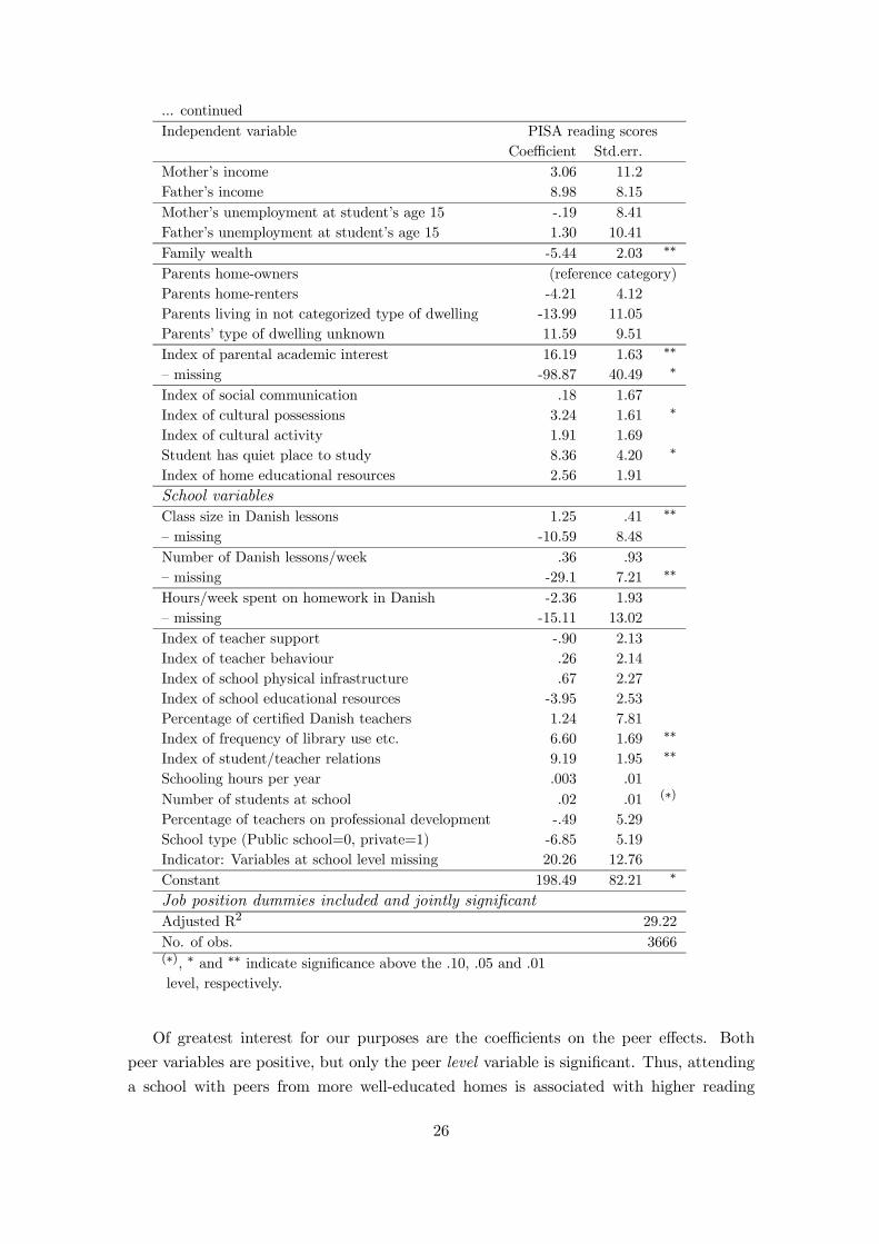
... continuedIndependent variable PISA reading scores

Coefficient Std.err.Mother’s income 3.06 11.2Father’s income 8.98 8.15Mother’s unemployment at student’s age 15 -.19 8.41Father’s unemployment at student’s age 15 1.30 10.41Family wealth -5.44 2.03 ∗∗

Parents home-owners (reference category)Parents home-renters -4.21 4.12Parents living in not categorized type of dwelling -13.99 11.05Parents’ type of dwelling unknown 11.59 9.51Index of parental academic interest 16.19 1.63 ∗∗

— missing -98.87 40.49 ∗

Index of social communication .18 1.67Index of cultural possessions 3.24 1.61 ∗

Index of cultural activity 1.91 1.69Student has quiet place to study 8.36 4.20 ∗

Index of home educational resources 2.56 1.91School variablesClass size in Danish lessons 1.25 .41 ∗∗

— missing -10.59 8.48Number of Danish lessons/week .36 .93— missing -29.1 7.21 ∗∗

Hours/week spent on homework in Danish -2.36 1.93— missing -15.11 13.02Index of teacher support -.90 2.13Index of teacher behaviour .26 2.14Index of school physical infrastructure .67 2.27Index of school educational resources -3.95 2.53Percentage of certified Danish teachers 1.24 7.81Index of frequency of library use etc. 6.60 1.69 ∗∗

Index of student/teacher relations 9.19 1.95 ∗∗

Schooling hours per year .003 .01Number of students at school .02 .01 (∗)

Percentage of teachers on professional development -.49 5.29School type (Public school=0, private=1) -6.85 5.19Indicator: Variables at school level missing 20.26 12.76Constant 198.49 82.21 ∗

Job position dummies included and jointly significantAdjusted R2 29.22No. of obs. 3666(∗), ∗ and ∗∗ indicate significance above the .10, .05 and .01level, respectively.

Of greatest interest for our purposes are the coefficients on the peer effects. Both

peer variables are positive, but only the peer level variable is significant. Thus, attending

a school with peers from more well-educated homes is associated with higher reading

26

scores. An increase in the average educational background of one’s peers by one year is

associated with an increase of one’s reading scores by almost 5 points on the PISA scale,

which amounts to 5% of the standard deviation of the scale. Stated alternatively, moving

a student from a class with a mean peer background of 9 years of parental schooling

(corresponding to compulsory education) to a class with a mean of 16 years of schooling

will increase that student’s achievement level by 35 points — or 37% of the standard

deviation of the scale. Compared to important family effects, the peer effect is important in

size. Students from households with a mother with a vocational education have predicted

reading scores that are 37 points lower than their counterparts who have a mother with

a university degree. Here, the peer group effect of moving from a peer group with mean

parental education of 9 years to a peer group where this number is 16 is of the same size

as the effect of own parental education by the same amount, which is remarkable.

Peer effects may be represented not only through the mean ability of classmates, but

also via the standard deviation in the abilities of classmates. The results on the peer

heterogeneity variable in Table 4 suggest that a student’s achievement level is higher,

when the heterogeneity of abilities within the classroom is greater suggesting that mixing

ability types generates educational benefits. However, the effect is imprecisely estimated

and thus not statistically significant different from zero.

While the primary interest of this study is on peer effects, let’s have a brief look at

the results for the control variables, anyway. Most of the estimated coefficients of these

variables are statistically significant and are usually in the direction one might expect

a priori. For example, parental education and occupation (not shown), not being the

youngest child, having fewer siblings, and attending a bigger school are positively related

to test scores — results typical of the literature. Also, female students have higher predicted

scores on average, as do native speakers. The effect of growing up with only one natural

parent is negative, but not (strongly) significant. Also, counterintuitively, being an only

child is associated with lower reading scores, while the effect of having many siblings is also

negative. Apparently, there is some ”optimal” number of siblings, while being an only child

might reflect some other factors in the family that have resulted in the decision not to have

more children (e.g. (female) career decisions, personal/family problems). Interestingly,

while income is not related to test scores, wealth is, but negatively so. We suspect this to

be a result of the somewhat problematic way of assessing family wealth in the PISA data.

The ”wealth” variable has been derived from students’ reports on the availability, in their

home, of a dishwasher, a room of their own, educational software, a link to the Internet;

and the number of cellular phones, television sets, computers, motor cars and bathrooms

at home. We suspect these factors not to be good indicators of family wealth in the case

of Denmark. Also, we know that the PISA index on family wealth has been constructed

in a way so its mean is 0 and its standard deviation is 1 in the total OECD sample. In

our Danish subsample, the mean is .53, while the standard deviation is only .74. Thus,

there is a comparably high level of ”wealth” as measured by the PISA index, but only

27

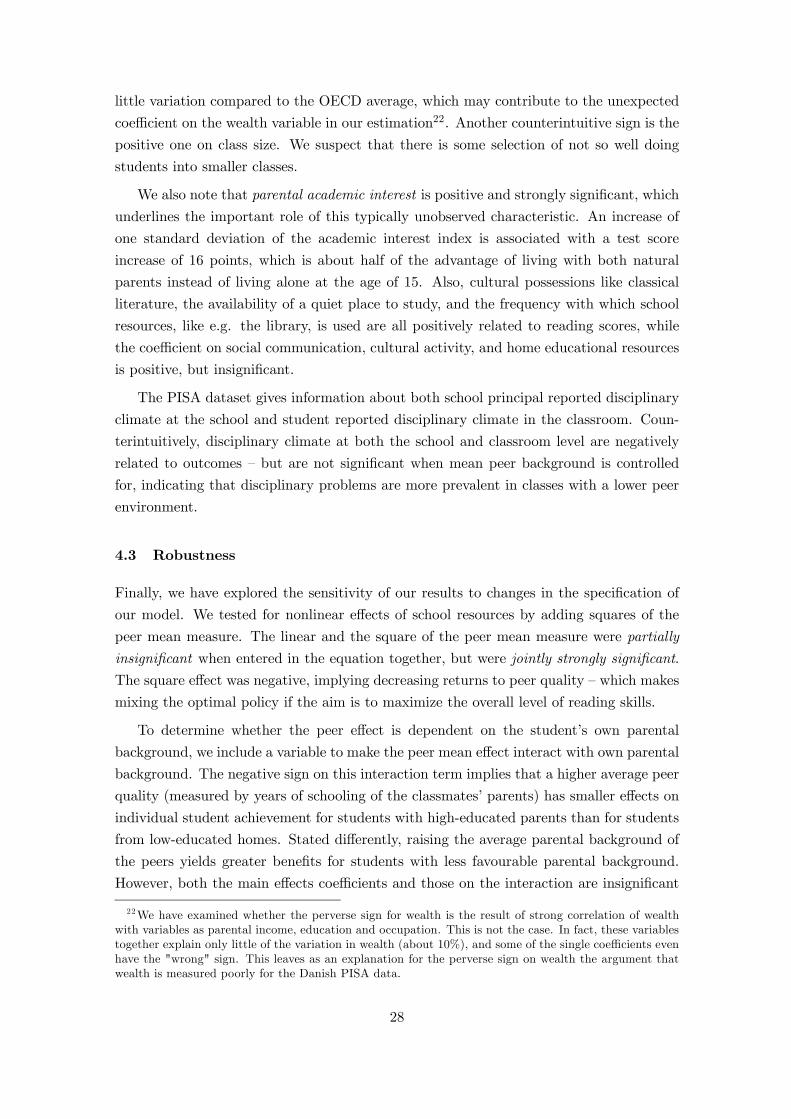
little variation compared to the OECD average, which may contribute to the unexpected

coefficient on the wealth variable in our estimation22. Another counterintuitive sign is the

positive one on class size. We suspect that there is some selection of not so well doing

students into smaller classes.

We also note that parental academic interest is positive and strongly significant, which

underlines the important role of this typically unobserved characteristic. An increase of

one standard deviation of the academic interest index is associated with a test score

increase of 16 points, which is about half of the advantage of living with both natural

parents instead of living alone at the age of 15. Also, cultural possessions like classical

literature, the availability of a quiet place to study, and the frequency with which school

resources, like e.g. the library, is used are all positively related to reading scores, while

the coefficient on social communication, cultural activity, and home educational resources

is positive, but insignificant.

The PISA dataset gives information about both school principal reported disciplinary

climate at the school and student reported disciplinary climate in the classroom. Coun-

terintuitively, disciplinary climate at both the school and classroom level are negatively

related to outcomes — but are not significant when mean peer background is controlled

for, indicating that disciplinary problems are more prevalent in classes with a lower peer

environment.

4.3 Robustness

Finally, we have explored the sensitivity of our results to changes in the specification of

our model. We tested for nonlinear effects of school resources by adding squares of the

peer mean measure. The linear and the square of the peer mean measure were partially

insignificant when entered in the equation together, but were jointly strongly significant.

The square effect was negative, implying decreasing returns to peer quality — which makes

mixing the optimal policy if the aim is to maximize the overall level of reading skills.

To determine whether the peer effect is dependent on the student’s own parental

background, we include a variable to make the peer mean effect interact with own parental

background. The negative sign on this interaction term implies that a higher average peer

quality (measured by years of schooling of the classmates’ parents) has smaller effects on

individual student achievement for students with high-educated parents than for students

from low-educated homes. Stated differently, raising the average parental background of

the peers yields greater benefits for students with less favourable parental background.

However, both the main effects coefficients and those on the interaction are insignificant

22We have examined whether the perverse sign for wealth is the result of strong correlation of wealthwith variables as parental income, education and occupation. This is not the case. In fact, these variablestogether explain only little of the variation in wealth (about 10%), and some of the single coefficients evenhave the "wrong" sign. This leaves as an explanation for the perverse sign on wealth the argument thatwealth is measured poorly for the Danish PISA data.

28

(however, they are jointly significant), suggesting that the effects are intertwined and

cannot credibly be estimated separately. We also wanted to estimate results on subsamples

divided by parental education, but the sample size was too small. The coefficients on the

peer variables were mostly insignificant and did not show any clear pattern.

In the existing literature, a range of variables have been used to proxy for the peer

environment at schools, e.g. the racial composition, and the share of students from two-

parent families. In reality, the peer environment at school is composed of many factors. As

it is not obvious which variables to use as a proxy for peer quality, we have experimented

with a range of characteristics. Using alternative measures of peer effects reinforces the

earlier results. Whether we use the mean and variance of parental occupational status, the

father’s education, the share of bilingual students in the class, or the share of students

living with both natural parents as our peer group indicator, we tend to find significant

mean peer effects with the ”right” sign and an insignificant peer heterogeneity effect.

4.4 Quantile regression results

Ordinary least squares methods estimate effects at the mean. By calculating regressions for

different quantiles, it is possible to explore the entire shape of the conditional distribution.

As will be shown, the quantile regression results suggest some important differences across

different points in the conditional distribution of reading scores.

The partial derivative of the conditional quantile of y with respect to one of the

regressors is to be interpreted as the marginal change in the θth conditional quantile

due to a marginal change in x. One should be cautious in interpreting this result. It

does not imply that a person who happens to be in the θth quantile of one conditional

distribution will also find himself at the same quantile had his x changed. But this is

mainly a problem with dummy explanatory variables, where a marginal change is from 0

(the lowest possible value) to 1 (the highest possible value). In the present study, both

variables of main interest are continuous, making this potential problem less severe.

Results from the estimation of quantile regressions at the 10th, 25th, 50th, 75th and

90th conditional percentile are presented in the Appendix23. In Figure 2, we report only

the coefficients on the main parameters of interest to this study — the peer level and peer

heterogeneity. The 90% confidence bounds are also plotted. The thin lines show the

OLS estimate and its confidence bands. Homogeneity in the peer level and heterogeneity

effect over the conditional test score distribution would imply that it is possible to draw

a horizontal line through the point estimates at different quantiles. However, in Figure 2

the point estimates suggest a pattern of effects that are larger in magnitude at the lower

quantiles as compared to the higher quantiles. The quantile regression (QR) coefficients do

clearly show a decreasing trend over the distribution suggesting that having good peers

23Estimates were calculated using the sqreg procedure of STATA version 7.0.

29

Peer Mean

-10

-5

0

5

10

15

20

.1 .25 .5 .75 .9

Peer Heterogeneity

-10

-5

0

5

10

15

20

.1 .25 .5 .75 .9

Figure 2: Quantile regression results for peer variables

is more important for low achievers than for high achievers. A test for the equality of

coefficients at the 1th and 9th decile suggests that the effects are significantly different at

the 10% level. A similar trend is present in the results for the heterogeneity of the peers

in the classroom. However, while the effect of the average peer quality in the classroom

remains positive and significant over most of the test score distribution, the effect of peer

heterogeneity is only weakly significant at the 10% level for the two lowest quantiles, and

is insignificant — and even turning negative — for higher quantiles. These results indicate

that low achievers profit from a heterogenous classroom, while the effect for high achievers

is not significantly different from zero.

Combining the results on peer level and class heterogeneity gives some suggestive policy

advice. The QR coefficients show a decreasing trend over the distribution suggesting that

having good peers is more important for low achievers than for high achievers making

mixing the preferable policy if the overall aim is to maximize average student performance.

However, increasing the ability mix does not only mean reducing disparities of the average

educational background of classrooms, but does necessarily also imply increasing classroom

heterogeneity. The peer level effect and the classroom heterogeneity effect are intertwined.

As the heterogeneity coefficient is positive and weakly significant for weak readers, while

being insignificantly different from zero for the upper part of the distribution, together

with the result that the effect from good peers is more effective at the lower quantiles,

suggests that mixing is the optimal policy for maximizing overall achievement.

It is important to stress that this solution is not pareto-optimal. However, when the

aim of the social planner is to maximize overall reading scores, the marginal products must

be equated across students at different points of the conditional test score distribution.

As the results show, the marginal product from a better peer group is higher at lower

quantiles than at higher quantiles. Equating marginal products by increased mixing will

therefore increase the overall reading performance.

30

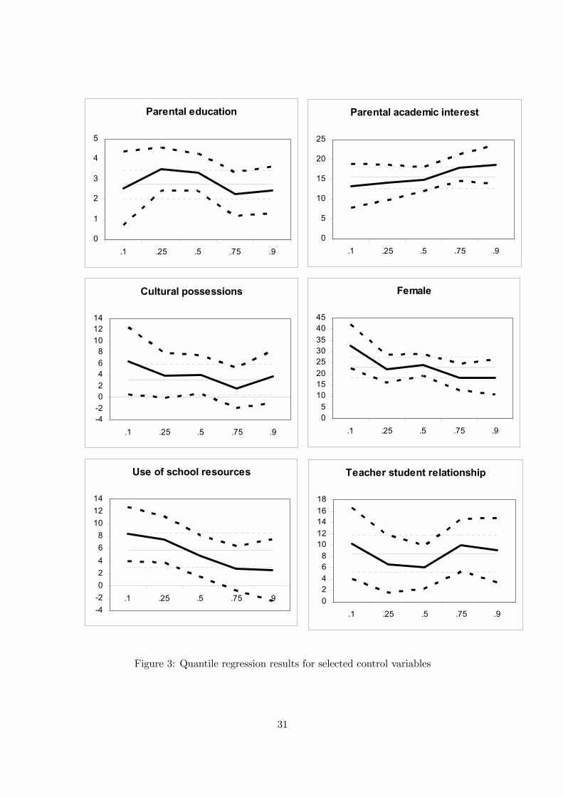
Parental academic interest

0

5

10

15

20

25

.1 .25 .5 .75 .9

Female

051015202530354045

.1 .25 .5 .75 .9

Use of school resources

-4-202468101214

.1 .25 .5 .75 .9

Cultural possessions

-4-202468101214

.1 .25 .5 .75 .9

Teacher student relationship

024681012141618

.1 .25 .5 .75 .9

Parental education

0

1

2

3

4

5

.1 .25 .5 .75 .9

Figure 3: Quantile regression results for selected control variables

31

As the peer variables are of main interest in this paper, and the OLS results for the

control variables have been reported in some detail, we will confine our discussion to only

a few of the covariates. A full results table is provided in the Appendix. Figure 3 shows

quantile regression results for six important control variables.

The effect of parental education on reading scores fluctuates somewhat around the

OLS estimate (shown with thin lines), but without any clear pattern and it does not leave

the OLS confidence interval24. The same is true for the index of parental academic interest

(upper right panel of Figure 3), but here the pattern is a steady increase of the effect over

the reading score distribution, suggesting that parental academic interest is an important

determinant of reading scores for students over the whole test score distribution, but

the effect seems to be more important for better readers. Interestingly, the opposite is

true for cultural possessions (middle left panel), which are significantly positive related to

reading scores only for weak readers, while the effect at the upper end of the distribution is

insignificant. The middle right panel of Figure 3 shows that girls read better than boys over

the whole range of the distribution, but the effect is particularly important at the lower

tail, where the quantile regression point estimate is outside the OLS confidence interval,

indicating that the effect of being a girl on reading scores may not be constant across the

conditional distribution. The effect of using school resources like the library, the Internet

etc. frequently (lower left panel) is positive and significant only at the lower end of the

conditional test score distribution, while the effect is close to zero for the higher quartiles

(0.75 and above). Apparently, especially weak readers profit from school resources over

and above classroom teaching. Interestingly, the teacher student relationship (lower right

panel) seems to be more important at both extremes of the test score distribution than

for average students: both weak and strong readers respond strongly to teacher student

relations, while students in between seem to be more independent from the relationship

with their teachers.

In several panels in Figure 3, quantile regression estimates lie at some point outside the

confidence intervals for the OLS regression, suggesting that the effects of these covariates

may not be constant across the conditional distribution of the independent variable. How-

ever, formal testing suggests that the coefficients for the first and last quantile estimated

is significantly different only for gender.

To recall, quantile regression techniques estimate peer effects at different values of the

conditional test score distribution. This means that when we talk about "weak readers",

we do not necessarily refer to students with low (absolute) test scores, but to students

reading less well than we would expect them to according to their background charac-

teristics. Thus, "weak readers" are, e.g., students from well-educated homes, who read

less well than the average student with well-educated parents. However, for policy pur-

poses, we are usually interested in students being poor readers unconditional on their

24For simplicity of the exposition of results, the parental education dummies were recoded into a con-tinuous variable indicating the number of years of schooling attained by the parent with most schooling.

32

Residuals

WLEREAD89.27 887.31

-338.841

291.493

Figure 4: Unconditional versus conditional reading scores

background. It is thus useful to examine, how unconditionally poor readers are related

to conditionally poor readers. If we, e.g., can show that the conditionally poor readers

are typically identical with the unconditionally poor readers, then, our quantile regression

results can be transferred directly to the unconditional distribution of test scores. To

find out about the relationship between the conditional and unconditional distribution,

we plot the residuals from the OLS regression (=conditional test scores) against raw test

scores in Figure 4. Unconditional and conditional test scores are closely related, which

illustrates the tendency of the conditionally poor readers to be identical with those who

get low raw test scores. This means that all results extracted above for the conditional

distributions are generally valid for the unconditional distribution, too. This relationship

makes our results much more easy to interpret for policy advice.

5 Conclusion

We investigated empirical peer group effects in the Danish, non-selective, school system.

Ordinary Least Squares results (mean effects) showed that there are sizeable positive

effects of attending school with peers with better educated parents. However, it could not

be shown that the heterogeneity of the classroom affects reading scores.

Also, our findings indicate for whom peers may matter, not just whether or not they

matter on average. The paper uses quantile regressions to describe effects at different

points of the conditional test score distribution. Quantile regressions provide "snap-shots"

at different points of a conditional distribution and, thus, are a parsimonious way of

describing the whole distribution. The estimation of education production functions at

several points of the test scores distribution revealed several interesting aspects that would

33

not be apparent by just examining a single regression equation, such as the mean. Quantile

regression results suggest that there may be differential peer group effects at different

points in the conditional test score distribution. Generally, peer group effects are stronger

at the lower end of the conditional test score distribution, confirming the suggestion in

the peer literature that low achievers are dependent learners. Such differences in the peer

effect is probably due to students with an educationally rich home environment, being

likely to do relatively well in most school environments. In contrast, the performance of

students from more educationally impoverished backgrounds may depend more heavily on

school factors as e.g. teacher quality, school resources, and their classmates.

Thus, quantile regression evidence reveals that the effect is stronger for weak readers.

This suggests, together with the insignificance of the coefficient on classroom heterogeneity

for the upper end of the conditional distribution of test scores that mixing, rather than

ability grouping of students, is preferable, when the aim is to maximize overall reading

performance.

In this paper, we show how our rich set of controls (we add variables form the PISA

dataset and administrative data to the usual set of controls) decreases the peer effect

coefficients compared to results from estimations with a smaller set of controls. This shows

that the comprehensive dataset we use eliminates bias due to selection of better students

into high-quality peer groups. However, while the bias is reduced, we cannot be sure that

it is eliminated entirely. Also, having only data on reading skills as outcome measure of

schooling, limits the scope of our results, if peer effects with respect to achievement in

other subjects (e.g. math or science) differ from peer effects for reading skills. With the

future release of data for the next PISA waves (PISA 2003, 2006) which will focus on

mathematical (2003) and science skills (2006), analyses on whether peer effects differ over

subjects will be feasible.

Finally, the peer effects we estimated are those present in a system with the deliber-

ate policy not to be selective. Results could change, when ability grouping became the

favoured policy approach, because this would constitute a shift in the educational system,

with an entire range of possible accompanying changes. E.g. the psychological effect of

being placed in a low ability track, the effect on teacher moral, teaching practices and

curriculum changes, when ability grouping becomes a policy rather than a feature that is

a product of differences in location pattern across different groups of families. How a fun-

damental change in the education system would affect the mean and distribution of test

scores will depend crucially on the particular features of the system to be implemented.

34

References

[Andrews, D. W., and M. Buchinsky (2000)] A three-step method for choosing the num-

ber of bootstrap repetitions. Econometrica 67, 23—51.

[Andrews, D. W., and M. Buchinsky (2001)] Evaluation of a three-step method for choos-

ing the number of bootstrap repetitions. Journal of Econometrics. Volume 103, Issues

1-2 , July 2001, 345-386.

[Angrist, J. and V. Lavy (1999)] Using Maimonides’ Rule to Estimate the Effect of Class

Size on Scholastic Achievement. Quarterly Journal of Economics, CXIV, May, 533-

75.

[Argys, L.M.; Rees, D.I. and D.J. Brewer (1996)] Detracking America’s Schools: Equity

at Zero Costs?; Journal of Policy Analysis and Management, 15, 4, 623-645.

[Behrman, J. R.; and M. R. Rosenzweig (2002)] Does Increasing Women’s Schooling

Raise the Schooling of the Next Generation? American Economic Review (March)

323-334.

[Benabou, R. (1993)] Workings of a City; Location, education, and production. Quarterly

Journal of Economics, 434 (August): 619-652.

[Benabou, R. (1996)] Heterogeneity, Stratification and Growth: Macroeconomic Implica-

tions of Community Structure and School Finance. American Economic Review, 86

(June): 584-609.

[Berglas, E.; and D. Pines (1981)] Clubs, local public goods and transportation models.

Journal of Political Economy, 15, 141-162.

[Betts, J.; and D. Morell (1999)] The Determinants of Undergraduate Grade Point Aver-

age — The Relative Importance of Family Background, High School Resources, and

Peer Group Effects. The Journal of Human Resources, 34, 2, 268-293.

[Betts, Julian; and Jamie L. Shkolnik (2000)] The Effects of Ability Grouping on Student

Achievement and Resource Allocation in Secondary Schools; Economics of Education

Review, 19, 1-15.

[Boozer, M.A.; and S.E. Cacciola (2001)] Inside the ”Black Box” of Project STAR: Esti-

mation of Peer Effects Using Experimental Data; Discussion Paper No. 832, Eco-

nomic Growth Center, Yale University.

[Brueckner, J.K.; and K. Lee (1989)] Club theory with a peer-group effect. Regional Sci-

ence and Urban Economics, 19, 399-420.

[Buchinsky, M. (1998)] Recent Advances in Quantile Regression Models: A Practical

Guideline for Empirical Research. Journal of Human Resources 33(1):88-126.

35

[Card, D. and A. Krueger (1992)] Does School Quality Matter? Returns to Education

and the Characteristics of Public Schools in the US; Journal of Political Economy,

100, 1-40.

[Caucutt, E. M. (2001)] Peer group effect in applied general equilibrium. Economic The-

ory, 17, 25-51.

[Caucutt, E.M. (forthcoming)] Educational vouchers when there are peer group effects —

size matters. International Economic Review.

[Danish National PISA report (2001)] Expectations and Skills ["Forventninger og

færdigheder"], in Danish with an English summary. AKF, DPU, SFI. Copenhagen,

Denmark.

[de Bartolome, C.A.M. (1990)] Equilibrium and Inefficiency in a Community Model with

Peer Group Effects. Journal of Political Economy 98 (Feb. 1990), 110-133.

[Eide, E.; and M. Showalter (1998)] The Effect of School Quality on Student Perfor-

mance: A Quantile Regression Approach; Economics Letters, 58, 345-350.

[Epple, D.; Newlon, E.; and R. Romano (2002)] Ability tracking, school competition, and

the distribution of educational benefits. Journal of Political Economy, 83, 1-48.

[Epple, D.; and R.E. Romano (1998)] Competition between public and private schools,

vouchers and peer group effects. American Economic Review 88 (May 1998) 33-62.

[Falk, A. and A. Ichino (2003)] Clean Evidence on Peer Pressure. IZA Discussion Paper

No. 732.

[Feinstein, L. and J. Symons (1999)] Attainment in Secondary School; Oxford Economic

Papers 51, 300-321.

[Fertig, Michael (2003)] Educational Production, Endogenous Peer Group Formation and

Class Composition — Evidence from the PISA 2000 Study; IZA DP No. 714.

[Figlio, D. and M. Page (2000)] School Choice and the Distributional Effects of Ability

Tracking: Does Separation Increase Equality?; NBER Working Paper No. 8055.

[Goldhaber, Dan D., and Dominic J. Brewer (1997)] Why Don’t Schools and Teachers

Seem to Matter? Assessing the Impact of Unobservables on Educational Productiv-

ity. Journal of Human Resources 32(3):505-523.

[Gould, W. (1992)] Quantile regression with bootstrapped standard errors. Stata Techni-

cal Bulletin 9: 19-21.

[Graversen, B. and E. Heinesen (2002) ] The Effect of School Resources on Educational

Attainment: Estimates for Different Sets of Controls and Different Subgroups of

Pupils; manuskript.

36

[Hallinan, Maureen (1990)] The Effects of Ability Grouping in Secondary Schools: A Re-

sponse to Slavin’s Best-Evidence Synthesis; Review of Educational Research 60 501-

504.

[Hanushek, E.A. (1986)] The Economics of Schooling: Production and Efficiency in Public

Schools; Journal of Economic Literature, 24, 114-177.

[Hanushek, E.A. (1996)] School Resources and Student Performance. In: Gary Burtless

(ed.), Does Money Matter? The Effect of School Resources on Students’ Achieve-

ment and Adult Success (Washington, D.C.: The Brookings Institution), pp. 43-73.

[Hanushek, E. A. (2001)] Does Peer Ability Affect Student Achievement? NBERWorking

Paper 8502.

[Hanushek, E. A. (2002)] Publicly Provided Education. In Alan J. Auerbach and Martin

Feldstein (eds.), Handbook of Public Economics, Amsterdam: North-Holland, 2047-

2143.

[Hanushek, Eric A.; Kain, John F.; Markman, Jacob M.; and Steven G. Rivkin (2003)]

Does Peer Ability Affect Student Achievement? Journal of Applied Econometrics

(forthcoming 2003).

[Henderson, V.; Miezkowski, P.; and Y. Sauvageau (1978)] Peer group effects and educa-

tional productions functions. Ottawa, Canada: Economic Council of Canada.

[Hoxby, Caroline (2000)] Peer Effects in the Classroom: Learning from Gender and Race

Variation; NBER Working Paper No. 7867.

[Koenker, R.; and G. Basset (1978)] Regression Quantiles; Econometrica, 46, 1, 33-50.

[Koenker, R.; and G. Basset (1982)] Robust Test for Heteroscedasticity Based on Regres-

sion Quantiles. Econometrica, 50(1): 43-61.

[Krueger, Alan B. (1999)] Experimental Estimates of Education Production Functions.

Quarterly Journal of Economics, 114(2): 497-532.

[Lavy, V. (1999)] Externalities and Efficiency Effects of Class Heterogeneity on Student

Scholastic Achievement; manuscript, Department of Economics, Hebrew University,

Jerusalem, Israel.

[Levin, J. (2001)] For Whom the Reductions Count: A Quantile Regression Analysis of

Class Size and Peer Effects On Scholastic Achievement; Empirical Economics, 26,

221-246.

[Nechyba, T.J. (1999)] School finance induced migration patterns: The impact of private

school vouchers. Journal of Public Economic theory, 1, (Jan.) 5-50.

37

[Nechyba, T.J. (2000)] Mobility, targeting and private school vouchers. American Eco-

nomic Review, 90.

[Oakes, J. (1992)] Can Tracking Research Inform Practice? Technical, Normative, and

Political Considerations. Educational Researcher, 21, 12-21

[Oakes, J. (1997)] Ability Grouping and Tracking in Schools. In: International Encyclo-

pedia of the Sociology of Education, L. J. Saha, ed.; 395-401.

[OECD (2001a)] Knowledge and Skills for Life — First Results from PISA 2000; OECD,

Paris.

[OECD (2001b)] PISA 2000 Technical Report; OECD, Paris.

[OECD (2002)] Reading for Change — Performance and Engagement Across Countries —

Results from PISA 2000; OECD, Paris.

[Rangvid, B.S. (2003)] Evaluating Private School Quality in Denmark. Working Paper

No. 03-2; Aarhus School of Business, Denmark.

[Robertson, D.; and J. Symons (1996)] Do Peer Groups Matter? Working Paper; Centre

for Economic Performance, London School of Economics and Political Science.

[Rogers, (1992)] Quantile regression standard errors. Stata Technical Bulletin 9: 16-19.

[Sacerdote, B. (2001)] Peer Effects with Random Assignment: Results for Dartmouth

Roommates; Quarterly Journal of Economics, 116,1, 681-704.

[Slavin, Robert (1990)] The Effects of Ability Grouping in Secondary Schools: A Best

Evidence Synthesis; Review of Educational Research 60, 471-499.

[Summers, A.; and B. Wolfe (1977)] Do Schools Make a Difference?; American Economic

Review 76, 639-652.

[Tiebout, C. (1956)] A Pure Theory of Local Public Expenditures. Journal of Political

Economy, 64: 416-24.

[Wilson, K. (2002)] The effects of school quality on income; Economics of Education Re-

view, 21, 579-588.

[Zimmer, R.W. and E.F. Toma (2000)] Peer Effects in Private and Public Schools Across

Countries; Journal of Policy Analysis and Management, 19(1): 75-92.

[Zimmerman, D.J. (1999)] Peer Effects in Academic Outcomes: Evidence from a Natural

Experiment; Discussion Paper 52, Williams College.

38

Appendix

Table A1: Quantile regression full results tabelDecile 0.1 0.25 0.5 0.75 0.9Independent variable Coef. Std. Coef. Std. Coef. Std. Coef. Std. Coef. Std.Peer variablesMean parental education of peers (years) 9.284 3.076 8.069 2.332 5.649 1.953 4.423 2.227 1.826 2.505Std.dev. of parental education of peers 6.821 4.032 4.727 2.867 1.119 2.247 -.025 2.659 -3.112 3.144Individual and family backgroundMale (reference category)Female 33.758 5.564 24.147 4.302 21.431 3.205 17.768 3.765 21.696 4.755Student’s age at test 7.124 9.937 10.760 8.049 6.908 6.540 10.553 6.644 6.117 8.693Ethnic Dane (reference category)Immigrant -35.813 24.508 -25.668 18.949 -16.842 15.687 -.455 14.903 -3.592 16.854Parents immigrated -52.810 32.749 -11.309 22.007 -8.224 13.904 -28.499 14.906 -13.910 31.360Does not speak Danish at home -45.832 20.636 -47.013 14.680 -50.428 12.224 -39.527 12.204 -44.640 13.707Number of brothers/sisters -4.256 3.169 -2.546 2.422 -3.148 1.950 -3.258 2.166 2.409 2.931Student is only child -19.180 13.597 -18.049 10.395 -17.389 9.272 -9.180 8.584 7.320 10.524Student is oldest child (reference category)Student is middle child -.807 8.452 5.756 6.387 -.966 6.368 -.542 5.924 -3.563 7.151Student is youngest child -12.111 6.335 -4.446 5.454 -6.906 3.864 -9.951 4.412 -6.010 5.256Student lives in nuclear family (reference category)... lives with single mother -8.436 9.551 -1.045 7.507 -8.222 6.050 5.695 7.423 -2.402 9.439... with mother and stepdad -4.283 9.168 -4.608 7.495 -4.715 5.884 -4.539 6.382 -15.869 8.839... with single dad .020 15.346 -4.439 19.679 11.291 11.562 -4.319 11.476 -6.237 16.516... with father and stepmum -14.297 18.908 -8.736 15.384 -8.105 12.781 -1.610 13.734 -7.746 20.757... without parents (parents together) -30.257 35.650 -9.622 36.239 -14.938 30.649 -25.967 25.850 -30.762 34.596... without parents (parents not together) -39.161 46.370 30.973 27.543 25.594 22.357 21.691 17.781 -11.054 27.179Student’s mother was teen at birth -13.033 19.313 -10.064 13.033 -15.616 10.511 -20.122 13.733 -.571 16.052Student’s father was teen at birth 18.641 32.924 48.268 31.361 17.691 15.859 2.028 24.403 -17.153 24.584Mother: unskilled (reference category)

- high-school degree 36.38 12.44 25.732 10.055 15.865 9.328 7.995 10.186 32.411 14.717- vocational education 8.95 6.77 10.341 5.953 3.331 4.086 .367 4.762 -1.958 5.77- short college 14.64 13.03 5.605 11.149 2.692 9.525 15.511 11.606 11.977 11.086- long college 27.14 10.90 22.366 8.092 13.757 6.440 18.235 7.878 18.616 8.251- university 53.70 16.22 38.974 13.035 36.677 10.748 33.573 13.278 35.358 14.957- PhD 65.96 38.18 -1.374 35.879 -.911 39.067 15.678 47.522 -34.042 49.749

Father: unskilled (reference category)- high-school degree 23.89 19.11 28.515 10.555 19.247 12.473 27.900 10.674 42.090 12.509- vocational education 2.58 6.99 5.664 5.567 6.105 5.093 13.305 4.218 19.353 5.430- short college 8.51 13.64 16.454 10.230 18.437 10.889 21.598 8.280 19.341 10.712

(...continued)

... continued0.1 0.25 0.5 0.75 0.9

Coef. Std. Coef. Std. Coef. Std. Coef. Std. Coef. Std.Father: long college 23.91 9.68 25.774 7.868 23.527 8.295 22.635 7.112 21.960 9.075

- university 38.46 13.01 27.579 9.934 21.295 9.484 23.924 9.643 23.566 12.574- PhD -14.38 29.66 -46.312 43.918 -31.256 51.595 50.221 98.428 143.698 93.919

Mother’s income 27.9 27.5 3.96 18.6 -10.9 17.7 4.55 21.9 8.83 24.3Father’s income -1.62 14.9 1.11 1.16 2.69 9.90 10.9 11.8 6.22 13.8Mother’s unemployment at student’s age 15 14.761 13.862 -8.736 11.334 2.662 11.610 7.249 11.135 -1.522 11.492Father’s unemployment at student’s age 15 -6.557 26.777 -18.857 18.582 6.793 14.501 10.940 16.921 23.406 16.097Family wealth -10.554 4.112 -6.095 2.825 -3.957 2.758 -3.516 2.564 -6.689 3.787Parents home-owners (reference category)Parents home-renters 4.425 7.558 -3.616 6.165 -9.277 4.851 -14.052 5.406 -13.877 8.246Parents living in not categorized type of dwelling -13.924 33.135 1.549 16.865 -8.334 11.319 -21.226 14.086 -28.503 19.069Parents type of dwelling unknown 15.496 13.012 7.392 10.719 4.237 12.831 -6.153 14.114 2.538 20.078Index of parental academic interest 13.324 3.406 14.337 2.753 14.818 1.820 17.321 2.072 17.359 2.615Index of social communication 3.229 3.377 1.960 2.435 1.373 2.149 -2.732 2.172 -2.118 2.946Index of cultural possessions 6.479 3.233 6.107 2.444 3.730 1.981 .541 2.073 1.423 2.513Index of cultural activity -.031 3.609 1.342 2.853 2.088 2.193 2.268 2.603 3.642 2.822Index of home educational resources 4.369 3.957 5.84 3.03 -.248 2.248 .631 2.556 5.536 2.885Student has quite place to study 15.714 11.015 6.820 5.821 6.660 5.864 5.738 5.583 4.921 7.135School variablesClass size in Danish lessons .093 .819 .847 .680 1.176 .588 .708 .523 1.483 .752Number of Danish lessons/week 1.180 1.551 .847 1.520 .948 1.148 -.129 1.050 -.887 1.573Hours/week spent on homework in Danish .303 3.996 -1.064 3.049 -.340 2.363 -3.263 2.767 -5.574 3.468Index of teacher support 1.167 3.919 1.773 3.777 1.586 2.802 -2.071 2.873 -3.276 3.877Index of teacher behaviour -.922 3.771 -.617 3.116 2.323 2.749 -.390 3.108 3.582 3.481Index of school physical infrastructure 1.673 4.217 4.432 3.182 2.041 2.628 -2.283 2.929 -8.519 3.876Index of school educational resources -6.127 4.849 -8.623 4.112 -3.572 3.057 -2.269 3.629 .072 4.050Percentage of certified Danish teachers 12.537 16.071 -2.630 11.641 -2.710 10.267 5.427 9.884 14.406 10.078Index of school resource use (e.g. library) 10.048 2.889 7.803 2.468 4.648 2.131 1.898 2.382 3.504 2.694Index of student/teacher relations 10.001 3.879 6.629 3.165 5.637 2.472 9.986 2.323 8.764 3.809Schooling hours per year -.024 .022 -.006 .018 .001 .015 .010 .015 .035 .020Number of students at school .016 .019 .010 .016 .026 .015 .026 .016 .019 .018Percentage of teachers on professional development 6.566 9.142 -8.598 7.970 -.195 7.268 -5.095 7.400 -11.338 9.765School type (Public school=0, private=1) -3.629 9.248 -4.689 7.657 -5.576 6.679 -9.067 7.379 -12.941 10.450No. of obs. 3666Bold (italic) figures indicate significance above the .05 (.10) level, respectively. Missing categories for parental education, ethnicity, parentalacademic interest, class size in Danish lessons, number of Danish lessons/week, hours/week spent on homework in Danish, missing schoollevel variablesand a constant included. Job position dummies included and jointly significant.