Measurement Errors in Quantile Regression Models∗

Sergio Firpo† Antonio F. Galvao‡ Suyong Song§

June 30, 2015

Abstract

This paper develops estimation and inference for quantile regression models withmeasurement errors. We propose an easily-implementable semiparametric two-step es-timator when we have repeated measures for the covariates. Building on recent theoryon Z-estimation with infinite-dimensional parameters, consistency and asymptotic nor-mality of the proposed estimator are established. We also develop statistical inferenceprocedures and show the validity of a bootstrap approach to implement the methods inpractice. Monte Carlo simulations assess the finite sample performance of the proposedmethods. We apply our methods to the well-known example of returns to educationon earnings using a data set on female monozygotic twins in the U.K. We documentstrong heterogeneity in returns to education along the conditional distribution of earn-ings. In addition, the returns are relatively larger at the lower part of the distribution,providing evidence that a potential economic redistributive policy should focus on suchquantiles.

Key Words: Quantile regression; measurement errors, returns to education

JEL Classification: C14, C23, J31

∗The authors would like to express their appreciation to Roger Koenker, Yuya Sasaki, Susanne Schennach,and Liang Wang for helpful comments and discussions. All the remaining errors are ours.†Sao Paulo School of Economics, FGV E-mail: sergio.firpo@fgv.br‡Department of Economics, University of Iowa, W284 Pappajohn Business Building, 21 E. Market Street,

Iowa City, IA 52242. E-mail: antonio-galvao@uiowa.edu§Department of Economics, University of Iowa, W360 Pappajohn Business Building, 21 E. Market Street,

Iowa City, IA 52242. E-mail: suyong-song@uiowa.edu

1 Introduction

Quantile regression (QR) models have provided a valuable tool in economics as a way of

capturing heterogeneous effects that covariates may have on the outcome of interest, exposing

a wide variety of forms of conditional heterogeneity under weak distributional assumptions.

Under some assumptions on the unobservable factors, QR can also be interpreted as providing

a structural relationship between the outcome of interest and its observable and unobservable

determinants. Also importantly, QR provides a framework for robust inference when the

presence of outliers is an issue.

Measurement errors (ME) have important implications for the reliability of general stan-

dard estimation and testing. Variables used in empirical economic analysis are frequently

measured with error, particularly if information is collected through one-time retrospective

surveys, which are notoriously susceptible to recall errors. If the regressors are indeed sub-

ject to classical ME, it is well known that the slope coefficient of the ordinary least squares

(OLS) estimator is inconsistent. In the one regressor case (or multiple uncorrelated regres-

sors), under standard assumptions, the OLS is biased toward zero, a problem often denoted

as attenuation (see, e.g., Carroll et. al. (2006) and references therein for an overview of ME

models).

Recently, the topic of ME in variables has received considerable attention in the QR

literature. As in the OLS case, the standard QR estimator has been shown to be inconsistent

in the presence of ME (see, e.g., Montes-Rojas (2011)). He and Liang (2000) consider

the problem of estimating QR coefficients in errors-in-variables models, and propose an

estimator in the context of linear and partially linear models. Chesher (2001) studies the

impact of covariate ME on quantile functions using a small variance approximation argument.

Schennach (2008) discusses identification of a nonparametric quantile function under various

settings when there is an instrumental variable measured on all sampling units. Identification

and estimation for general quantile functions are based on Fourier transforms and previous

results for nonlinear models (see, e.g., Schennach, 2007). Wei and Carroll (2009) propose a

method for a linear QR model that corrects bias induced by the ME by constructing joint

estimating equations that simultaneously hold for all the quantile levels. More recently,

Torres-Saavedra (2013) and Hausman, Luo, and Palmer (2014) study ME in the dependent

variable of QR models. We refer to Ma and Yin (2011), Wang, Stefanski, and Zhu (2012),

and Wu, Ma, and Yin (2014) for other recent developments in QR models with ME. Thus, in

1

the analysis of QR with mismeasured covariates, it has been common to employ estimation

methods that either impose parametric restrictions on nuisance functionals or use exogenous

information as those provided by instrumental variables (see, e.g., Wei and Carroll (2009),

Schennach (2008), and Chernozhukov and Hansen (2006)). Nevertheless, methods relying

on parametric assumptions are very sensitive to misspecification of such conditions, which

are indeed relevant for inference as the asymptotic variance typically requires estimation of

conditional densities. In addition, finding exogenous instrumental variables is known to be

a nontrivial task in most economic models.

This paper contributes to both the QR and ME branches of the literature by developing

estimation and inference methods for QR models in the presence of ME in the covariates.

This is achieved by exploring repeated measures of the true regressor. Identification and

estimation of conditional mean regression models with repeated measures of the true regres-

sor have already been studied in Li (2002), Schennach (2004) and Hu and Sasaki (2015),

among others. However, to the best of our knowledge, there has yet been no attempt to

develop estimation and inference for QR models using repeated measures of the true re-

gressor. This paper bridges this gap. We propose a simple, easily-implementable, and well-

behaved two-step semiparametric estimation procedure that preserves the semiparametric

distribution-free and heteroscedastic features of the model. The first step employs a gen-

eral nonparametric estimation of the density function. The second step uses the estimated

densities as weights in a weighted QR estimation. We establish the asymptotic properties

of the two-step estimator, assuming that the conditional densities satisfy smoothness condi-

tions and can be estimated at an appropriate nonparametric rate. We also develop practical

statistical inference, and propose testing procedures for general linear hypotheses based on

the Wald statistic. To implement these tests in practice the critical values are computed

using a bootstrap method. We provide sufficient conditions under which the bootstrap is

theoretically valid, and discuss an algorithm for its practical implementation. Our method

leads to a simple algorithm that can be conveniently implemented in empirical applications.

Compared to the existing procedures for QR models with ME, our approach has several

distinctive advantages. First, our method does not assume global linearity at all quantile

levels for the estimation of the conditional density function as in Wei and Carroll (2009).

Such feature makes our procedure applicable to any τ -quantile of interest, thus relaxing the

requirement of a joint estimation and providing more flexibility. Second, our algorithm is

computationally simple and easy to implement in practice because estimation of the weights

2

does not require recursive algorithms allowing the weights for all observations to be obtained

from one single step. As a result, the quantile estimate is attained by minimizing only one

single convex objective function at the quantile of interest. Third, the methodology does

not rely on instrumental variables. Therefore, information from outside the model is not

necessary for identification. Finally, our estimated weights exhibit a property of uniform

consistency, implying that it is feasible to establish both the consistency and asymptotic

normality of the resulting estimators of the parameters of interest. Hence, the method

provides standard inference and testing procedures.

Monte Carlo simulations assess the finite sample properties of the proposed methods.

We evaluate the estimator in terms of empirical bias, standard deviation, and mean squared

error, and compare its performance with methods that are not designed for dealing with

ME issues. The experiments suggest that the proposed approach performs relatively well in

finite samples and effectively removes bias induced by ME.

Our procedure will hopefully be useful for those empirical settings based on QR models

in which ME in the independent variables is a concern because the method does provide

intuitive and practical ways of handling the problem. To motivate and illustrate the applica-

bility of the methods, we revisit and analyze the important example of returns to education

on earnings. The QR approach is an important tool in this example because it allows us to

capture the heterogeneity in the returns to education along the conditional wage distribu-

tion. At the same time, endogeneity induced by ME has been extensively discussed in the

returns to education example, as misreporting in the number of schooling years is a gen-

uine concern (Card (1995), Card (1999), and Harmon and Oosterbeek (2000)). Within that

framework, finding valid and strong instrumental variables to solve the endogeneity problem

is not, in general, an easy task (see, e.g., Card (1999)). Thus, our method is a natural

alternative solution to the ME problem when repeated measures on educational achievement

are available.

In our empirical example we use a data set on female monozygotic twins in the U.K.

that had been previously used in Bonjour et al. (2003) to study the problem of returns to

education. Bonjour et al. (2003) use the information on one twin to obtain an instrumental

variable for schooling years on the other twin. Amin (2011) points out that the results in

Bonjour et al. (2003) are largely affected by outlier observations and revisited the problem

using QR. He uses the same data on twins and apply the instrumental variables method-

3

ology described in Arias, Hallock, and Sosa-Escudero (2001). We compare our results with

those from Bonjour et al. (2003) and Amin (2011). Our empirical findings exemplify and

support the idea that the proposed methods are a useful alternative to existing approaches

in economic applications in which ME is an important concern. We document strong hetero-

geneity in returns to education along the conditional distribution of earnings. In addition,

the returns are relatively larger at the lower part of the distribution, providing evidence that

a potential economic redistributive policy should focus on such quantiles.

The rest of the paper is organized as follows. Section 2 presents the model and discusses

identification of the parameters of interest in presence of ME. Section 3 proposes the two-step

QR estimator. Section 4 establishes the asymptotic properties of the estimator. Inference

is discussed in Section 5. Section 6 presents the Monte Carlo experiments. In Section 7, we

illustrate empirical usefulness of the the new approach by applying to returns to education.

Finally, Section 8 concludes the paper.

2 Model and identification

2.1 Model

We first introduce the model studied in this paper. Given a quantile τ ∈ (0, 1), we define

the following quantile regression (QR) model,

Yi = X>i β0(τ) + Z>i δ0(τ) + εi(τ), (1)

where Yi is the scalar dependent variable of interest, Xi is a vector of potentially-mismeasured

covariates, Zi is a vector of correctly-observed covariates, and εi(τ) is the innovation term

whose τ -th quantile is zero conditional on (Xi, Zi). The structural parameters of interest are

θ0(τ) = (β0(τ), δ0(τ)). In general, each β0(τ) and δ0(τ) will depend on τ , but we assume τ

to be fixed throughout the paper and suppress such a dependence for notational simplicity.

Suppose (Yi, Xi, Zi) are i.i.d. random variables defined on a complete probability space

(Ω,F , P ). Define the population objective function for the τ -th conditional quantile as

Q(β0, δ0) := E[ψτ (Yi −X>i β0 − Z>i δ0)[Xi Zi]

]= 0, (2)

where ψτ (u) := (τ − Iu < 0) with the indicator function I·. When the true covariates

(X,Z) are observed, β0 and δ0 can be consistently estimated from the standard quantile

4

regression model with sample analog of Q(β, δ) in (2) as

Qn(β, δ) :=1

n

n∑i=1

ψτ (Yi −X>i β − Z>i δ)[Xi Zi] = 0. (3)

The presence of the indicator function in the above equation implies that the solution may

not be an exact zero. It is usual to write this estimator as a minimization problem, and then

use linear programming to solve the optimization. Thus, the above moment condition is a

slight abuse of notation, but since everything else involving observed data is an estimating

equation that will have a zero, we will use the estimating equation nomenclature. For more

details on Z-estimator with non-smooth objective functions, see He and Shao (1996, 2000).

2.2 Measurement error bias and its solution

Under the assumption of perfectly-measured regressors, the solution of equations (3) can

be shown to produce consistent estimates of (β0, δ0). Nevertheless, it is commonly observed

that researchers have to use the regressor X measured with error. Using mismeasured X

in the standard QR estimation in (3) induces a substantial bias in the estimates of the

coefficients of interest (see, e.g., He and Liang, 2000). Thus, estimation of the standard QR

model under measurement errors (ME) leads to inconsistent estimates. To overcome this

drawback we propose a methodology that makes use of repeated measures. Both variables

are mismeasured observables of the true covariate.

Suppose that true covariate X is unobservable due to ME. Instead, a researcher observes

two error-laden measurements which are noisy measures of X and defined as follows

X1i = Xi + U1i

X2i = Xi + U2i,

where U1i and U2i are ME. Therefore, the observed random variables are (Yi, X1i, X2i, Zi),

and one seeks to estimate the parameters (β0, δ0).

We show how to use information from the measures X1 and X2 to obtain consistent

estimates of the parameters of interest. For that purpose, it is useful to rewrite Q(β, δ) as a

5

function of the density function as well as (β, δ):

Q(β0, δ0, f0) := E[ψτ (Y −X>β0 − Z>δ0)[X Z]]

=

∫ψτ (y − x>β0 − z>δ0)[x z] · fY XZ(y, x, z)dydxdz

=

∫ψτ (y − x>β0 − z>δ0)[x z] · fX|Y Z(x | y, z)fY Z(y, z)dydxdz

= E

[∫x

ψτ (Y − x>β0 − Z>δ0)[x z] · fX|Y Z(x | Y, Z)dx

](4)

= 0,

where fY XZ(y, x, z) and fY Z(y, z) are the joint density of (Y,X,Z) and (Y, Z), respectively,

and where fX|Y Z(x | y, z) ≡ f0 is the conditional density of X given (Y, Z). By replacing

the outer expectation with its empirical counterpart, we write the sample analog of the

population objective function (4) as:

Qn(β, δ, f) :=1

n

n∑i=1

∫x

ψτ (Yi − x>β − Z>i δ)[x Zi] · fX|Y Z(x | Yi, Zi)dx (5)

= 0.

The integration in (5) makes the function continuous in its argument. The summand

of (5) is Ex[ψτ (Yi − x>β − Z>i δ)[x Zi] | Yi, Zi], the conditional mean of the original score

function given the observed Y and Z. Moreover, (5) is an unbiased estimating function,

that is, has mean zero, and will be the basis for constructing estimating equations to obtain

consistent estimates of the parameters of interest.

Therefore, one would solve the new estimating equation (5) to estimate the parameters

of interest. In empirical applications, however, the true conditional density fX|Y Z(x | y, z)is unknown and to implement the estimator (5) in practice one needs to replace it with

fX|Y Z(x | y, z), a consistent estimate of fX|Y Z(x | y, z). Thus, a (feasible) estimator would

first estimate fX|Y Z(x | y, z). The fitted density function from this step would be used to

estimate the coefficients of interest in a second step. Finally, with a consistent estimate

of the conditional density, (β0, δ0) can be consistently estimated. However, in general, the

conditional density is not stochastically identified due to the unobservability of the true X.

In a related model, Wei and Carroll (2009) make use of an iterative algorithm to obtain a

consistent estimator of the conditional density fX|Y X1(x | y, x1) in the presence of ME on X.1

1We note that their conditional density is slightly different from ours since there is mismeasured covariateX1 in their conditioning set.

6

They focus on model with one measurement of true X (here X1) and with no other observed

covariates Z for simplicity. Although their approach can be useful in some applications, it

has important technical challenges. First, in order to implement the estimator, one needs

to estimate the conditional density fX|Y X1(x | y, x1) which requires pre-specified parametric

form of fX|X1(x | x1). This suffers from potentially serious model misspecification. Second,

and related to the first problem, there is a problem to solve the estimating equations, since

estimating the conditional density fX|Y X1(x | y, x1) involves estimation of the entire pro-

cess β0(τ) over quantiles τ . In other words, the estimating equations in Wei and Carroll

(2009) need to be solved jointly for all the τ ’s, which increases the dimensionality of the

problem substantially and makes implementation considerably difficult. This is reflected in

the tractability of inference for their method.

In this paper, we propose a novel way to nonparametrically estimate the conditional

density without imposing assumptions on known distributions of the ME. Specifically, we

make use of the repeated measures, X1 and X2, and show that two mismeasured covariates

are sufficient to identify the conditional density in the presence of ME on the covariate. In

turn, the result guarantees consistent estimation of parameters of interest. The approach

with repeated measurements has been recently studied in the ME literature. Most of studies

have focused on i.i.d. measurement errors (e.g., Li and Vuong, 1998; Delaigle, Hall, and

Meister, 2008). We extend the literature by relaxing such strong conditions. We also extend

issues in smooth objective function of mean regression with ME (e.g., Schennach, 2004) to

a non-smooth objective function such as the QR.

In the next section we propose a procedure that yields a consistent estimator of (β0, δ0)

in (5). We develop a method for QR with measurement errors, which relies on estimating

the conditional density function nonparametrically. The method is a two-step estimator,

where in the first step we estimate the density nonparametrically and then in the second

step we employ a standard weighted QR procedure. Before we proceed to estimation, we

show an identification result for the density function which is essential in the estimation.

For expositional ease, we use fX|Y Z(x | y, z) and f(x | y, z) synonymously.

2.3 Conditional density

As described above, f(x | y, z) is an important element for the identification of the pa-

rameters of interest in the QR with ME. This section describes the identification of the

7

conditional density function f(x | y, z) which is required to compute the two-step estimator.

The identification is based on the assumption that repeated measures of the true regressor

are observed. We state the following assumptions to obtain the main identification result.

Assumption A.I: (i) E[U1 | X,U2] = 0; (ii) U2 ⊥ (Y,X,Z).

Assumption A.II: (i) E[|X|] < ∞; (ii) E[|U1|] < ∞; (iii) |E[exp(iζX2)]| > 0 for any

finite ζ ∈ R.

Assumption A.III: (i) sup(x,y,x1,z)∈supp(X,Y,Z) f(x | y, z) <∞; (ii) f(x | y, z) is integrable

on R for each (y, z) ∈ supp(Y, Z).

Assumption A.I imposes restrictions on the repeated measures of X. Assumption A.I (i)

requires conditional mean zero of ME on X1, but allows dependence of the ME and (X,U2).

Assumption A.I (ii) requires that ME on X2 is independent of true X as well as other

variables. However, it does not necessarily require zero mean of U2. Thus, our setting on

the repeated measures can be useful for an example such that there is a drift or trend in the

mismeasured covariates. Assumption A.II imposes mild restrictions on the existence of the

first moments of X and U1, and nonvanishing characteristic function of X2. These have been

commonly assumed in the deconvolution literature (see, e.g., Fan, 1991b; Fan and Truong,

1993). Assumption A.III is trivially satisfied in commonly-used conditional densities.

Let φ(ζ, y, z) ≡ E[eiζX | Y = y, Z = z] be conditional characteristic function of X given

Y and Z. The following theorem presents the identification of f(x | y, z).

Theorem 1 Suppose Assumptions A.I–A.III hold. Then, for (x, y, z) ∈ supp(X, Y, Z),

f(x | y, z) =1

2π

∫φ(ζ, y, z) exp(−iζx)dζ, (6)

where for each real ζ,

φ(ζ, y, z) =E[eiζX2 | Y = y, Z = z]

E[eiζX2 ]exp

(∫ ζ

0

iE[X1eiξX2 ]

E[eiξX2 ]dξ

).

Proof. See Appendix.

The theorem implies that conditional density f(x | y, z) can be written as a function of

purely-observed variables. For this, we use useful properties of Fourier transform. Namely, we

8

write f(x | y, z) as the inverse Fourier transform of φ(ζ, y, z). This simplifies identification

since φ(ζ, y, z) is easily identified from Assumptions A.I–A.III by removing the ME, U1

and U2, in the frequency domains (ζ, ξ). It is worth noting that the identification result is

similar to Kotlarski (1967) who identifies density of X from its repeated measurements by

assuming mutual independence of X, U1, and U2. Our approach rests on weaker assumptions

than their mutual independence, which is highlighted in condition A.I. As a result, the

proposed method can be applied to many interesting topics which allow for dependence

among variables and their ME.

2.4 Identification

Given the result in equation (6), we can rewrite Q(β, δ, f) as:

Q(β, δ, f) = E

[∫x

ψτ(Y − x>β − Z>δ

)[x Z] · fX|Y Z(x | Y, Z)dx

]= E

[∫x

ψτ(Y − x>β − Z>δ

)[x Z] ·

(1

2π

∫ζ

φ(ζ, Y, Z) exp(−iζx)dζ

)dx

],

which does not depend on data on X. Thus, estimation of (β0, δ0) follows from solving a

feasible version of Qn(β, δ, f):

Qn(β, δ, f) =1

n

n∑i=1

∫x

ψτ(Yi − x>β − Z>i δ

)[x Zi] · fX|Y Z(x | Yi, Zi)dx,

where

fX|Y Z(x | Yi, Zi) =1

2π

∫ζ

φ(ζ, Yi, Zi) exp(−iζx)dζ,

and the only feature of this sample objective function that had not yet been presented is

φ, the estimate of φ, which is defined in the next section. In practice, as we discuss next,

we approximate integrals by sums, thus actual implementation solves a slightly different

objective function. By approximating the integral by a sum, we end up with a double sum

(on observations and on grid values of X). Importantly on that representation is the fact

that the estimates (β, δ) will be obtained by a weighted QR, whose weights will be given by

the estimate fX|Y Z .

9

3 Estimation

Given the identification condition in equation (6) of Theorem 1, we are able to estimate

the structural parameters of interest, (β0, δ0). We propose a semiparametric estimator that

involves two-step estimation. Implementation of the estimator is simple in practice. In

the first step, one estimates the nuisance parameter, the conditional distribution, using a

nonparametric method which requires no optimization. In the second step, by plugging-in

these estimates, a general weighted quantile regression (QR) is performed.

3.1 Estimation of nuisance parameter

In this subsection we discuss the estimation of the nuisance parameter in the first step,

i.e., the conditional density f(x | y, z). It is important to note that the proposed density

estimation is novel in the literature and makes use of repeated measures and nice properties

of Fourier transform.

The estimation of the nuisance parameter is very important step for implementation of

the proposed estimator in practice. We propose a nonparametric method to estimate the

density consistently. To obtain a consistent estimator of f(x | y, z), we adapt the class

of flat-top kernels of infinite order proposed by Politis and Romano (1999). Consider the

following assumption.

Assumption A.IV: The real-valued kernel x→ k(x) is measurable and symmetric with∫k(x)dx = 1, and its Fourier transform ξ → κ(ξ) is bounded, compactly supported, and

equal to one for |ξ| < ξ for some ξ > 0.

From Assumption A.IV, we allow for a kernel of the form (see, e.g., Li and Vuong, 1998)

k(x) =sin(x)

πx, (7)

with its Fourier transform such that

κ(hxζ) =

∫1

hxk( xhx

)exp(iζx)dx, (8)

for a bandwidth hx. This flat-top kernels of infinite order has the property that its Fourier

transform is equal to one over [−1, 1] interval and zero elsewhere, which guarantees that

the bias goes to zero faster than any power of the bandwidth. We note that the ill-posed

10

inverse problem occurs when one tries to invert a convolution operation. This is true to our

proposed estimator because it is divided by a quantity which converges to zero as frequency

parameter goes to infinity by Riemann-Lebesgue lemma. By estimating the numerator using

the kernel whose Fourier transform is compactly supported, one can guarantees that the

ratio is under control. This is because that the numerator can decay to zero before the

denominator converges to zero. This compact support of the Fourier transform of the kernel

can be easily implemented by preserving most of the properties of the original kernel. For

instance, one can transform any given kernel k into a modified kernel k with compact Fourier

support by using a window function that is constant in the neighborhood of the origin and

vanishes beyond a given frequency.

The following theorem summarizes the result.

Theorem 2 Suppose Assumptions A.I–A.III hold, and let k satisfy Assumption A.IV.

For (x, y, z) ∈ supp(X, Y, Z) and hx > 0, let

f(x | y, z;hx) ≡∫

1

hxk

(x− xhx

)f(x | y, z)dx. (9)

Then we have

f(x | y, z;hx) =1

2π

∫κ(hxζ)φ(ζ, y, z) exp(−iζx)dζ. (10)

Proof. See Appendix.

Let hn ≡ (hxn, h(2)n ) with h

(2)n ≡ (hyn, h

zn) be a set of smoothing parameters. Let E[·] denote

a sample average, i.e., 1n

∑ni=1[·]. Finally, we introduce a consistent nonparametric estimator

of f(x | y, z) motivated by Theorem 2.

Definition 2.3 The estimator of f(x | y, z) is defined as

f(x | y, z;hn) ≡ 1

2π

∫κ(hxnζ)φ(ζ, y, z, h(2)

n ) exp(−iζx)dζ, (11)

for hn → 0 as n→∞, where

φ(ζ, y, z, h(2)n ) ≡ E[eiζX2 | Y = y, Z = z]

E[eiζX2 ]exp

(∫ ζ

0

iE[X1eiξX2 ]

E[eiξX2 ]dξ

).

11

The above estimator is useful to compute the structural parameters of interest. Since it

has an explicit closed form, it requires no optimization routine unlike other likelihood-based

approaches. Estimation of conditional mean, E[eiζX2 | Y = y, Z = z], can be achieved via

any nonparametric method. For instance, one might use popular kernel estimation with

khn(·) ≡ h−1n k (·/hn) (e.g., Epanechnikov kernel) defined as

E[eiζX2 | Y = y, Z = z] ≡E[eiζX2khyn(Y − y)khzn(Z − z)]

E[khyn(Y − y)khzn(Z − z)]].

3.2 Estimation of the structural parameters

This section describes the general estimator for QR models with ME. The estimator can be

obtained in two steps. Given the identification condition in equation (5) and the estimator of

the density function described in the previous section, we are able to estimate the structural

parameters of interest. We propose a Z-estimator that involves two-step estimation. We

estimate the parameters of interest, θ0 = (β0, δ0) for a selected τ of interest, from the

following two steps:

Step 1. Estimate f(xj | Yi, Zi;h) for each i-th observation and j-th grid as in equation

(5) where j ∈ J ≡ 1, 2, . . . ,m with m number of grids for approximating the numer-

ical integral. The choice of kernels and bandwidths are provided in Definition 2.3 above.

The integrals in equation (11) are performed using the fast Fourier transforms (FFT) algo-

rithm. Well-behaving performance of the algorithm is guaranteed by the smoothness of the

characteristic function φ(·) and the finiteness of the moments.

Step 2. Then, to compute equation (5) in practice, we have to make a numerical

approximation to the integral over x. We do this via translating the problem into a weighted

quantile regression problem. Let x = (x1, x2, ..., xm) is a fine grid of possible xj values, akin

to a set of abscissas in Gaussian quadrature. For each τ , θ(τ) = (β(τ), δ(τ)) can be computed

by solving

n∑i=1

m∑j=1

ψτ (Yi − x>j β − Z>i δ)[xj Zi] · f(xj | Yi, Zi;h) = 0, (12)

where f(xj | Yi, Zi;h) is obtained from Step 1. The weighted quantile regression of Yi on

xj and Zi with corresponding weights f(xj | Yi, Zi;h) can be readily computed using the

function called “rq” in R package quantreg.

12

The asymptotic properties of the estimator given in equation (11) and also of (β(τ), δ(τ)),

in equation (12), are established in Section 4 below.

4 Asymptotic properties

This section investigates the large sample properties of the proposed two-step estimator.

While these methods seem similar to the ones discussed by Wei and Carroll (2009), the

novel estimation of the conditional density function raises some new issues for the asymptotic

analysis of the estimator. First, we establish the asymptotic results for the estimator of the

conditional density function given in (11). Second, we establish consistency and asymptotic

normality of the two-step estimator in (12).

4.1 Asymptotic properties of the density estimator

In this subsection we establish the asymptotic properties of the density function estimator in

equation (11). Let µ(ζ) ≡ E[eiζX ], ω1(ζ) ≡ E[eiζX2

], and χ(ζ, y, z) ≡

∫eiζx2fX2Y Z(x2, y, z)dx2.

We impose the following assumptions.

Assumption B.I: (i) There exist constants C1 > 0 and γµ ≥ 0 such that

|Dζ lnµ(ζ)| =∣∣∣∣Dζµ(ζ)

µ(ζ)

∣∣∣∣ ≤ C1(1 + |ζ|)γµ ;

(ii) There exist constants Cφ > 0, αφ ≤ 0, νφ ≥ 0, and γφ ∈ R such that νφγφ ≥ 0 and

sup(y,z)∈supp(Y,Z)

|φ(ζ, y, z)| ≤ Cφ(1 + |ζ|)γφ exp(αφ|ζ|νφ),

and if αφ = 0, then γφ < −1;

(iii) There exist constants Cω > 0,αω ≤ 0, νω ≥ νφ ≥ 0, and γθ ∈ R such that νωγω ≥ 0 and

min inf(y,z)∈supp(Y,Z)

|χ(ζ, y, z)|, |ω1(ζ)| ≥ Cω(1 + |ζ|)γω exp(αω|ζ|νω).

Assumption B.II: (i) E[|X1|2] <∞; (ii) E[|X1||X2|] <∞; (i) E[|X2|] <∞.

Assumption B.III: sup(y,z)∈supp(Y,Z)) |f(y, z)− f(y, z)| = Op

((lnn)1/2

(nhyhz)1/2+∑

s=y,z(hs)2)

.

These assumptions are standard for nonparametric deconvolution estimators because

their rates of convergence will depend on the tails of the Fourier transforms (see, e.g., Fan,

13

1991b; Fan and Truong, 1993). The literature commonly adopts two types of smoothness

assumptions: ordinary and super smoothness. Ordinary smoothness admits a Fourier trans-

form whose tail decays to zero at a geometric rate |ζ|γ, γ < 0 whereas super smoothness

admits a Fourier transform whose tail decays to zero at an exponential rate exp (α |ζ|γ),α < 0, γ > 0.2 Assumption B.I simultaneously imposes ordinary and super smoothness

conditions.3 Assumption B.II imposes mild moment restrictions required for consistency

results. Assumption B.III imposes a standard condition on nonparametric estimator of the

joint density of f(y, z).

The next result establishes the asymptotic properties of the density function estimator.

Theorem 3 Let Assumptions A.I–IV and B.I–III hold. Then for (x, y, z) ∈ supp(X, Y, Z)

and h > 0 satisfying max(hyn)−1, (hzn)−1 = O (nη) and

(hxn)−1 = O((lnn)1/νω−η

)if νω 6= 0,

(hxn)−1 = O(n(1−20η)/2(γµ−γω)

)if νω = 0,

for some η > 0, we have

sup(x,y,z)∈supp(X,Y,Z)

|f(x | y, z;h)− f(x | y, z)|

= O((

(hx)−1)γB exp

(αB((hx)−1

)νB))+Op

(n−1/2

(max

(1 + (hx)−1

)δL , (hyhz)−1) (

1 + (hx)−1)γL exp

(αL((hx)−1

)νL)) ,with αB ≡ αφξ

νφ, νB ≡ νφ, γB ≡ γφ + 1, αL ≡ αφ1νφ=νω − αω, νL ≡ νω, γL ≡ 1 + γφ − γω,

and δL ≡ 1 + γµ.

Proof. See Appendix.

The theorem above establishes a consistency and uniform convergence rate of the pro-

posed estimator. The conditions on the bandwidths are imposed to guarantee that asymp-

totic behavior of the linear approximation of the expression f(x | y, z;h) − f(x | y, z) is

2The typical examples of ordinarily smooth functions are uniform, gamma, symmetric gamma, Laplace(or double exponential), and their mixtures. Normal, Cauchy, and their mixtures are super smooth functions.

3A term exp (α1 |ζ|ν1) is omitted in Assumption B.I (i) with merely a small loss of generality since lnµ (ζ)is indeed a power of ζ.

14

essentially determined by a variance term since a nonlinear remainder term is asymptoti-

cally negligible. The result also shows that convergence rate depends on the tail behaviors of

the associated quantities. For instance, when χ(ζ, y, z) and ω1(ζ) in Assumption B.I is ordi-

narily smooth (i.e., νω = 0), one can choose small bandwidth so that resulting convergence

rate of the estimator is faster than when they are super smooth.

4.2 Asymptotic properties of the two-step estimator

In this subsection, we derive the asymptotic properties of the two-step estimator of param-

eters of interest. We establish its consistency and asymptotic normality.

4.2.1 Consistency

Consistency is a desirable property for most estimators. We wish to establish consistency of

the estimator θ = (β, δ) defined in equation (12), where f , given in (11), is an estimator of

f0 := f(x | y, z).

First, notice that from the estimating equation in (5) we have

Qn(β, δ, f) =1

n

n∑i=1

∫ψ(Yi − x>β − Z>i δ)(x Zi) · f(x | Yi, Zi) dx,

and its expectation is

Q(β, δ, f) = E

∫ψ(Yi − x>β − Z>i δ)(x Zi) · f(x | Yi, Zi) dx.

The estimator θ = (β, δ) is obtained by equating Qn(β, δ, f) to zero, where f is an estimator

of f0. Note that Q(β, δ, f0) = 0 if and only if (β>, δ>)> = (β>0 , δ>0 )> ∈ Θ.

Now we formally state the following sufficient conditions for the two-step estimator to be

consistent.

Assumption C.I: Qn(β, δ, f) = op(1).

Assumption C.II: X ∈ X , a compact set in Rdx .

Assumption C.III: E[|Z|] <∞.

15

Condition C.I defines the estimating equation (Z-estimator). Pakes and Pollard (1989)

and Chen, Linton, and Van Keilegom (2003) have similar assumptions. For a detailed dis-

cussion of this type of identification assumption, see, e.g., He and Shao (1996, 2000). C.II

imposes compactness for the true covariate. A similar assumption in the QR literature

appears in Chernozhukov and Hansen (2006). C.III only requires the first moment of the

well-measured regressor to be finite. A uniform law of large numbers for the first-step estima-

tor f(x | y, z) is standard in two-step estimation literature; see, e.g., Newey and McFadden

(1994). We note that this is straightforwardly satisfied by Theorem 3.

The following theorem derives consistency of the proposed two-step estimator, θ = (β, δ).

Theorem 4 Under assumptions C.I–C.III and conditions of Theorem 3, as n→∞

θp→ θ0.

Proof. See Appendix.

4.2.2 Weak convergence

Now we derive the limiting distribution of the two-step estimator in (12). We impose the

following assumptions for weak convergence.

Assumption G.I: Qn(β, δ, f) = op(n−1/2).

Assumption G.II: The conditional density gY (y | X = x, Z = z) is bounded and

uniformly continuous in y, uniformly in x and z over the support of (Y,X,Z).

Assumption G.III: Let Γ1 := EgY (X>β0+Z>δ0) | X,Z)(X>, Z>)>(X>, Z>) be positive

definite and Vn := var[Qn(θ0)]. There exists a nonnegative definite matrix V such that

Vn → V as n→∞.

Assumption G.IV: ||f − f0|| = op(n−1/4).

Assumption G.V: Z ∈ Z is compact.

Assumption G.VI: For some ε > 0, Fε = f : ||f − f0|| ≤ ε is uniformly bounded and

Donsker.

16

Condition G.I defines the estimator. It is slightly stronger than condition C.I but still

allows the right-hand side to be only approximately zero. This type of op(n−1/2) condition is

also assumed in Theorem 3.3 of Pakes and Pollard (1989) and Theorem 2 of Chen, Linton,

and Van Keilegom (2003). Conditions G.II and G.III are standard in the QR literature;

see, e.g., Koenker (2005). Condition G.IV imposes that the estimator of the nuisance

parameter converges at a rate faster than n−1/4. A similar condition appears in condition

(2.4) in Theorem 2 of Chen, Linton, and Van Keilegom (2003). Assumption G.V strengthens

C.III and imposes compactness on the well-measured regressor. Finally, condition G.VI

is similar to Chen, Linton, and Van Keilegom (2003) and Galvao and Wang (2015), and

guarantees that f is asymptotically well behaved. This condition is related to the stochastic

equicontinuity of the moment function associated with Qn. It allows for many nonparametric

estimators of the conditional density f0. Primitive conditions can be obtained through the

derivation of asymptotic normality of f , which requires finding a lower bound for the variance

of the estimator. In fact, an exact asymptotic rate of convergence can be obtained from the

assumption that the limiting behavior of the relevant Fourier transforms has a power law or

an exponential form; see e.g., Fan (1991a) for the kernel deconvolution estimator.

We note that Assumption G.IV is verifiable for particular examples through Theorem 3.

As shown in Theorem 3, the convergence rate is controlled by the smoothness of quantities

such as φ(ζ, y, z), χ(ζ, y, z), and ω1(ζ). Recall that φ(ζ, y, z) is the conditional density of

X given Y = y and Z = z (i.e., f(X | Y = y, Z = z)), the parameter of interest in the

first step; χ(ζ, y, z) is the conditional characteristic function of X2 given Y = y and Z = z,

weighted by the joint density of (Y, Z) (i.e., E[eiζX2 | Y = y, Z = z]f(y, z)); and ω1(ζ) is the

characteristic function of X2. Since ω1(ζ) = E[eiζX2 ] = E[eiζX ]E[eiζU2 ], the smoothness of

ω1(ζ) is determined by X and U2. Therefore, the rate of convergence depends on the possible

combinations of the smoothness of various quantities. For instance, if φ(ζ, y, z) is ordinarily

smooth and if χ(ζ, y, z) and ω1(ζ) are super smooth, a convergence rate of the form (lnn)−υ

for some υ > 0 is achieved. This case illustrates a very slow rate of convergence. On the other

hand, a faster convergence rate, n−υ for some υ > 0, which satisfies Assumption G.IV, can

be achieved when φ(ζ, y, z) is also super smooth. In addition, if all three quantities, φ(ζ, y, z),

χ(ζ, y, z), and ω1(ζ), are ordinarily smooth, the slow convergence problem is easily avoided.

Weak convergence of the two-step estimator, θ = (β, δ), is established in the following

result.

17

Theorem 5 Under Assumptions C.I–C.III, G.I–G.VI, and conditions of Theorem 3, as

n→∞

√n(θ − θ0) N(0,Λ)

for some positive definite matrix Λ = Γ−11 V Γ−1

1 .

Proof. See Appendix.

5 Inference

In this section, we turn our attention to inference in the quantile regression (QR) with mea-

surement errors (ME) model. Important questions posed in the econometric and statistical

literatures concern the nature of the impact of a policy intervention or treatment on the

outcome distributions of interest; for example, whether a policy exerts a significant effect, a

constant versus heterogeneous effect, or a non-decreasing effect. It is possible to formulate

a wide variety of tests using variants of the proposed method, from simple tests on a single

quantile regression coefficient to joint tests involving many covariates and distinct quantiles

simultaneously. We suggest a bootstrap-based inference procedure to test general linear

hypotheses.

5.1 Test statistic

General hypotheses on the vector θ(τ) can be accommodated by standard tests. The pro-

posed statistic and the associated limiting theory provide a natural foundation for the hy-

pothesis Rθ(τ) = r when r is known. The following are examples of hypotheses that may

be considered in the former framework.

Example 1 (No effect of the mismeasured variable). For a given τ , if there is no dynamic

effect in the model, then under H0 : β(τ) = 0. Thus, θ(τ) = (β(τ), δ(τ))>, R = [1, 0] and

r = 0.

Example 2 (Location shifts). The hypotheses of location shifts for β(τ) and δ(τ) can

be accommodated in the model. For the first case, H0 : β(τ) = β, so θ(τ) = (β(τ), δ(τ))′,

R = [1, 0] and r = β. For the latter case, H0 : δ(τ) = δ, so that R = [0, 1] and r = δ.

18

More general hypotheses are also easily accommodated by the linear hypothesis. Let

ζ = (θ(τ1)>, ..., θ(τm)>) and define the null hypothesis as H0 : Rν = r. This formulation

accommodates a wide variety of testing situations, from a simple test on single QR coefficients

to joint tests involving several covariates and distinct quantiles. Thus, for instance, we might

test for the equality of several slope coefficients across several quantiles.

Example 3 (Same mismeasured effect for two distinct quantiles). If there are the same

effects for two given distinct quantiles in the model, then under H0, β(τ1) = β(τ2). Thus,

ζ = (θ(τ1)>, ..., θ(τm)>) = (β(τ1), δ(τ1), β(τ2), δ(τ2))>, R = [1, 0,−1, 0] and r = 0.

Consider the following general null hypothesis for a given τ of interest

H0 : Rθ(τ)− r = 0,

where R is a full-rank matrix imposing q number of restrictions on the parameters, and r

is assumed to be a known column vector of q elements. Practical implementation of testing

procedures can be carried out based on the following statistic

Wn(τ) = Rθ(τ)− r. (13)

From Theorem 5, at given τ , and under the null hypothesis, it follows√n(Rθ(τ)− r)

N(0, RΛR′). If we are interested in testing H0, a Chi-square test could be conducted based

on the statistic in equation (13). However, to carry out practical inference procedures, even

for a fixed quantile of interest, to construct a Wald statistic one would need to first estimate

Λ consistently, and consequently nuisance parameters which depend on both the unknown θ0

and f0 in a complicated way. The estimation of Λ is potentially difficult because it contains

additional terms from the effect of θ on the objective function indirectly through f0. An

alternative method is to use the statistic Wn directly and the bootstrap to compute critical

values and also form confidence regions. Therefore, to make practical inference we suggest

the use of bootstrap techniques to approximate the limiting distribution.

5.2 Implementation of testing procedures

Practical implementation of the proposed tests is simple. To test H0 with known r, one needs

to compute the test statistics Wn(τ) for a given τ of interest. The steps for implementing

the tests are as following:

19

First, the estimates of θ(τ) are computed by solving the problem in equation (12). Second,

Wn(τ) is calculated by centralizing θ(τ) at r. Third, after obtaining the test statistic, it is

necessary to compute the critical values. We propose the following scheme. Take B as a

large integer. For each b = 1, . . . , B:

(i) Obtain the resampled data (Y bi , X

b1i, X

b2i, Z

bi ), i = 1, . . . , n.

(ii) Estimate θb(τ) and set W bn(τ) := R(θb(τ)− θ(τ)).

(iii) Go back to step (i) and repeat the procedure B times.

Let cB1−α denote the empirical (1 − α)-quantile of the simulated sample W 1n , . . . ,W

Bn ,

where α ∈ (0, 1) is the nominal size. We reject the null hypothesis if Wn is larger than cB1−α.

Confidence intervals for the parameters of interest can be easily constructed by inverting the

tests described above.

We provide a formal justification of the simulation method. Consider the following con-

ditions.

Assumption G.IB: For any δn ↓ 0, sup||f−f0||≤δn ||1n

∑ni=1 f(·)−E[f0(·)]|| = op∗(1/

√n).

Assumption G.IIB:√n 1n

∑ni=1[(τ − 1Yi < qτ0)(f ∗(·) − f(·))] converges weakly to a

tight random element G in L in P∗-probability.

Lemma 1 Under Assumptions C.I–C.III, G.IB–G.IIB and G.VI with “in probability”

replaced by “almost surely”, the bootstrap estimator of the θ0 is√n-consistent and

√n(θ∗ −

θ) N(0,Λ) in P∗-probability.

Proof. See Appendix.

Lemma 1 establishes the consistency of the bootstrap procedure. It is important to

highlight the connection between this result and the previous section. In fact, Lemma 1 shows

that the limiting distribution of the bootstrap estimator is the same as that of Theorem 5,

and hence the above resample scheme is able to mimic the asymptotic distribution of interest.

Thus, computation of critical values and practical inference are feasible.

20

6 Monte Carlo simulations

6.1 Monte Carlo design

In this section, we describe the design of a small simulation experiment that have been con-

ducted to assess the finite sample performance of the proposed two-step estimator discussed

in the previous sections. We consider the following model as a data generating process:

Yi = β1 + β2Xi + εi,

where ε ∼ N(0, 0.25), and β1 and β2 are the parameters of interest.4 We set them as

(β1, β2) = (0.5,−0.5). The true variable X is not observed by the researcher, and we use

additive forms of measurement errors (ME) to generate the mismeasured X as follows:

X1i = Xi + U1i,

X2i = Xi + U2i,

where we generate X ∼ N(0, 1), and we use a Laplace distribution density as L(0, 0.25)

to generate both measurement errors, U1 and U2. We compute and report results for the

proposed QR estimator. For comparison, we compute the density fX|Y using different pro-

cedures. First, we construct our proposed estimator to control for ME, using the variables

(Y,X1, X2), where the density is estimated by the Fourier Estimator. Second, we use the

variables (Y,X) to construct an “infeasible” kernel estimator of fX|Y in the first step. Fi-

nally, the variables (Y,X1) are used for “naive” kernel estimator of fX|Y which still suffers

from ME. For all estimators, we consider fourth-order Gaussian kernel. We approximate the

inner summation in equation (12) using Gauss-Hermite quadrature which is useful for the

indefinite integral. We perform 1000 simulations with n = 500 and n = 1000. We scan a

set of bandwidths for X and Y in order to find empirical optimal bandwidths in terms of

minimizing mean squared error.

6.2 Monte Carlo results

We report results for the following statistics of the coefficient β2: bias (B), standard deviation

(SD), and mean squared error (MSE). First of all, in order to illustrate the problem of ME

in practice, we consider a model estimation where the researcher ignores the ME problem

4For simplicity, the perfectly-observed covariate Z is absent here.

21

and performs a parametric median regression of Y on X1 without correcting for the ME in

X. This simple regression provides the bias of 0.1686, the standard error 0.02655 and the

MSE of 0.02586. These results highlight the importance of correcting for the ME problem.

Now we discuss and present the results for the nonparametric estimators with(out) correc-

tion of ME. Tables 1–3 report finite-sample performance of three different two-step estimators

at the median: (i) our proposed estimator (Fourier estimator); (ii) infeasible kernel estima-

tor; (iii) naive kernel estimator. These results are for n = 500, but the results for n = 1000

are similar. At the bottom of each table, B, SD, and MSE from optimal bandwidth are

reported. In Table 4 we vary the quantiles and present results for the different estimators

across different deciles with n = 1000.

Tables 1 - 3 Simulation Results

[ABOUT HERE]

Table 1 shows that the proposed estimator is effective in reducing the bias when true X

is measured with errors and repeated measures of the mismeasured covariate are available.

These results are comparable to the infeasible kernel estimator in Table 2. On the other

hand, the results in Table 3 from the naive kernel estimator ignoring ME in X show much

larger bias over all selected bandwidths. Therefore, our estimator outperforms the naive

kernel estimator in terms of both bias and MSE. The minimum MSE for our proposed

method is 0.00674 while the minimum MSE from the naive kernel estimator is 0.01008. This

result confirms that the methods proposed in this paper are beneficial in finite samples when

repeated measures of the mismeasured regressor are available to the researcher.

Table 4 reports finite-sample performance of three estimators over various quantiles with

n = 1000. For simplicity, we use the optimal bandwidths obtained from the simulation

results above. The results confirm that our proposed estimator performs well over different

level of quantiles.

Table 4 - Simulation Results

[ABOUT HERE]

22

7 Empirical application

This section illustrates the usefulness of the new proposed methods in an empirical example.

One of the most commonly studied topics in labor economics is the impact of education

on earnings. The problem of measuring returns to education is an important research area

in economics with a very large literature on the subject. For examples of comprehensive

studies, see, e.g., Card (1995), Card (1999), and Harmon and Oosterbeek (2000). The large

volume of research in this area has been explained by both the interest in the causal effect

of education on earnings and the inherent difficulty in measuring this effect. The difficulty

arises for several reasons. The classical one is the fact that unobserved factors, such as

ability is probably related to both educational level and earnings. In a mean regression

framework, if ability is positively correlated with both education and earnings, ordinary

least squares (OLS) will overestimate true causal impact of education on earnings. Finding

strong instrumental variables (IV) that are not correlated with unobserved ability is usually

a difficult task. Nevertheless, even when available, IV estimators do not necessarily produce

estimated coefficients of education that are significantly lower than those obtained by OLS.

A potential reason for these findings in the returns to education literature is that IV’s

are used for two simultaneous purposes: to correct for both an omitted variable bias (since

ability is unobservable) and measurement errors (ME) in reported schooling years. Educa-

tion measures are frequently measured with error, particularly if the information is collected

through one-time retrospective surveys, which are notoriously susceptible to recall errors,

(see, e.g., Ashenfelter and Krueger (1994), Kane, Rouse, and Staiger (1999), Bound, Brown,

and Mathiowetz (1999), and Black, Sanders, and Taylor (2003)). It is also known that ME

in a simple framework can provoke attenuation bias, thus OLS may not necessarily be over-

estimating the true returns to education if ME is a quantitatively more important problem

than omitting a covariate. Thus, it became important in that literature to understand what

is the isolated role of ME on the bias of estimated coefficients.

We use quantile regression (QR) methods to study returns to education. We accom-

modate possible heterogeneity on the returns to education in the earnings distribution by

applying QR. Indeed, this heterogeneity is not revealed by conventional least squares or two

stage least squares, while the QR approach constitutes a suitable way to investigate whether

the returns to education differ along the conditional wage distribution. In this paper, we

primarily focus on controlling for ME in education, even though the omitted variable bias

23

may be an important issue. To the best of our knowledge, there is no published work which

effectively controls for both omitted variable and ME in QR.5 Careful research is required

to control for both sources of endogeneity of education in the QR framework. We leave this

topic for future research.

Our QR method proposes a solution to the ME problem in education by using repeated

measures of the education variable. The literature on the returns to education has used

useful information on repeated measurements of education where one twin is asked to report

on both his/her own schooling and the schooling of the other twin (Ashenfelter and Krueger

(1994) and Bonjour et al. (2003)). This allows one to treat the information reported by the

other twin as a repeated measure of the true education. We therefore apply our method to a

data set on female monozygotic twins from the Twins Research Unit, St. Thomas’ Hospital

from the United Kingdom. Our data are taken from Bonjour et al. (2003) and Amin (2011).

The sample consists of 428 individuals comprising 214 identical twin pairs with complete

wage, age, and schooling information. The summary statistics are described in Table 5.

Table 5 - Summary Statistics

[ABOUT HERE]

The proposed QR estimator is designed to correct for the ME problem while exploring

heterogeneous covariate effects, and therefore provides a flexible method for the practical

analysis of returns to education. Thus, our objective is to estimate the following conditional

quantile function:

QWi(τ |edui, Zi) = β(τ)edui + Z>i δ(τ), (14)

where Wi is the earnings of individual i, edui is the true number of years of education

which is latent, and Zi is a vector of exogenous covariates. The parameters of interest are

(β(τ), δ(τ)). As mentioned earlier, if edui is subject to ME, and only edu1i and edu2i are

observed, standard QR estimates of β(τ) using edu1i or edu2i will be inconsistent. For the

practical implementation of the procedures, the dependent variable is the log of wage (Y ).

The independent variable subject to ME is education and the observed repeated measures

5Amin (2011) uses the average education of the twins as an additional covariate to proxy for omittedability bias and uses co-twin’s estimate of education as an instrument to control for ME in self-reportededucation. However, this procedure generates an issue of two mismeasured covariates which require twovalid instruments. Amin (2011) instruments both mismeasured covariates with reported education variables.However, there will be ME on those instruments, which makes the IV approach in QR invalid.

24

of true education are twin 1’s education (X1) and twin 2’s report of twin 1’s education (X2).

These Y , X1 and X2 are standardized to have mean zero and standard deviation one, for the

purpose of bandwidth selection. We use age and squared age as correctly-observed exogenous

covariates (Z).

Clearly, the model in equation (14) is very simple: ability has a monotonically positive

or negative impact on education return. However, as emphasized by Arias, Hallock, and

Sosa-Escudero (2001), QR provides a more flexible approach to distinguishing the effect of

education on different percentiles of the conditional earning distribution, being consistent

with a non-trivial and, in fact, unknown interaction between education and ability.

We compare the estimates using our proposed methods with those from the existing lit-

erature, in particular the results presented in Amin (2011) for QR and IV-QR. Amin (2011)

presents results for the parameter of interest using the two-stage QR estimator of Arias,

Hallock, and Sosa-Escudero (2001) and Powell (1983), where fitted value of education is es-

timated in the first stage and a QR of log of wage on the fitted value of education follows in

the second stage. However, for comparison purposes, we report estimates using the standard

IV-QR proposed by Chernozhukov and Hansen (2006). For this, we use the variable edu2

as an instrument for education edu1. The IV strategy is based on the assumption that the

co-twin’s education is strongly related to the other’s report of the co-twin’s education (i.e.,

IV) but the IV is independent of unobservable factors of earnings as well as measurement

errors (e.g. Chernozhukov and Hansen (2005)). We conjecture that the IV approach delivers

different estimates than our proposed ME estimator since they rely on different set of con-

ditions. Our method is particularly useful for the data set where it is unlikely that the IV is

independent of the regression error which contains ME on self-reported education, since the

IV is also mismeasured.6

Our results for the estimates of the returns to education coefficient are reported in Fig-

ures 1–4. The figures present results for the coefficients and confidence bands, for a range of

quantiles, for QR, IV-QR, and QRME, respectively. The shaded region in each panel repre-

sents the 95% confidence interval. In addition, the estimates for simple OLS and the IV-OLS

appear in the respective figures, with dashed red lines for confidence bounds. In Figure 1

we report standard QR and OLS estimates. The estimation strategy follows Koenker and

6We note that the independence condition implies independence between ME on the co-twin’s educationand the other’s report of the co-twin’s education. However, our approach requires a weaker assumption ofconditional mean zero as in Assumption A.I (i).

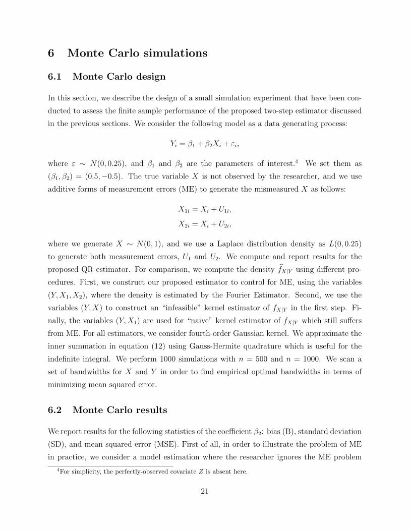
25

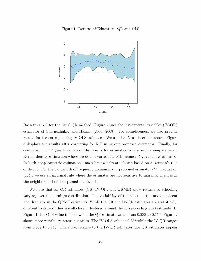
Figure 1: Returns of Education. QR and OLS

0.2 0.4 0.6 0.8

0.0

0.1

0.2

0.3

0.4

0.5

quantiles

coefficients

o

o

o oo

o o o o

o oo

oo

oo

o

o o oo

oo o o

o

o

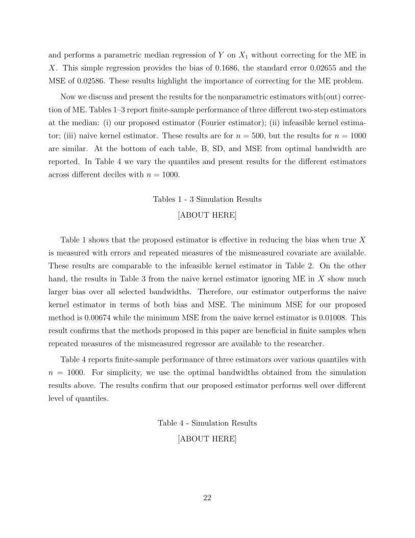
Bassett (1978) for the usual QR method. Figure 2 uses the instrumental variables (IV-QR)

estimator of Chernozhukov and Hansen (2006, 2008). For completeness, we also provide

results for the corresponding IV-OLS estimates. We use the IV as described above. Figure

3 displays the results after correcting for ME using our proposed estimator. Finally, for

comparison, in Figure 4 we report the results for estimates from a simple nonparametric

Kernel density estimation where we do not correct for ME; namely, Y , X1 and Z are used.

In both nonparametric estimations, most bandwidths are chosen based on Silverman’s rule

of thumb. For the bandwidth of frequency domain in our proposed estimator (hxn in equation

(11)), we use an informal rule where the estimates are not sensitive to marginal changes in

the neighborhood of the optimal bandwidth.

We note that all QR estimates (QR, IV-QR, and QRME) show returns to schooling

varying over the earnings distribution. The variability of the effects is the most apparent

and dramatic in the QRME estimates. While the QR and IV-QR estimates are statistically

different from zero, they are all closely clustered around the corresponding OLS estimate. In

Figure 1, the OLS value is 0.336 while the QR estimate varies from 0.288 to 0.356. Figure 2

shows more variability across quantiles. The IV-OLS value is 0.382 while the IV-QR ranges

from 0.539 to 0.243. Therefore, relative to the IV-QR estimates, the QR estimates appear

26

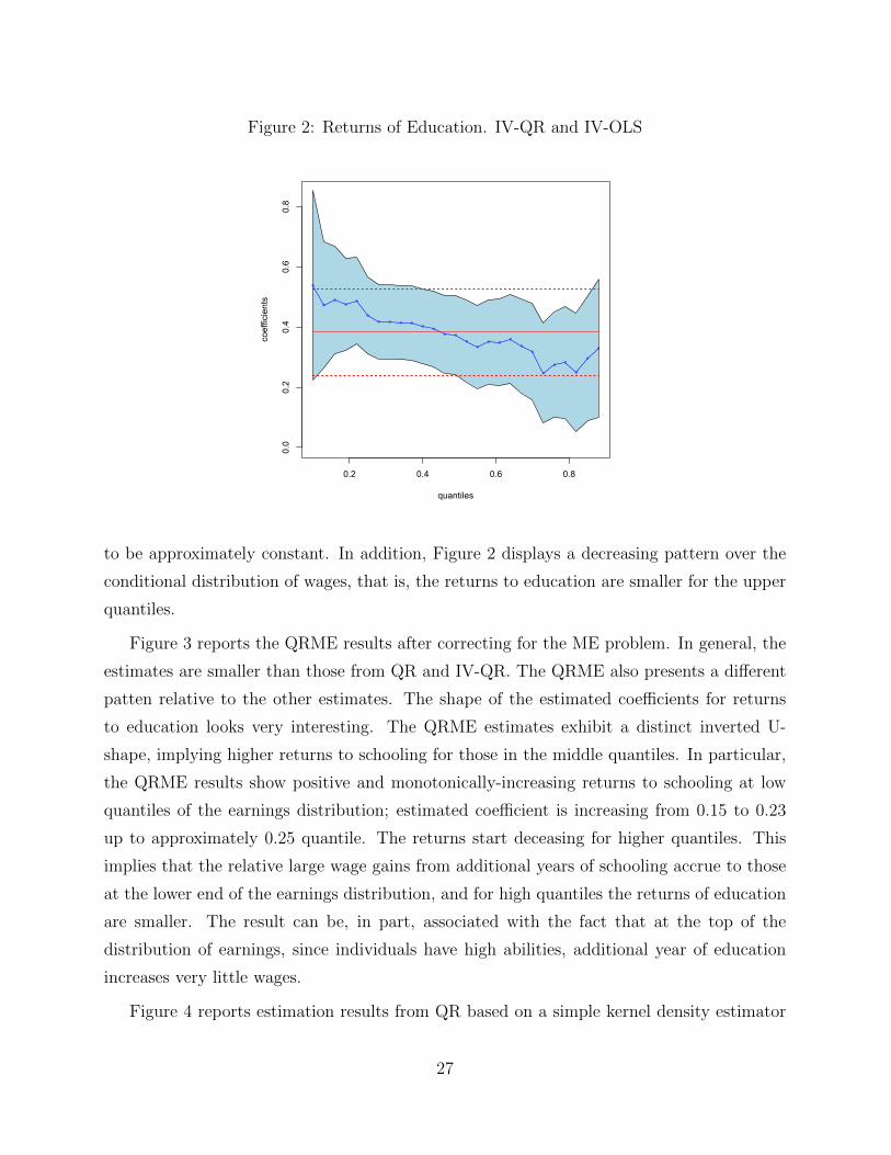
Figure 2: Returns of Education. IV-QR and IV-OLS

0.2 0.4 0.6 0.8

0.0

0.2

0.4

0.6

0.8

quantiles

coefficients

o

oo

oo

oo o o o

o oo o

oo

o oo

oo

o

o o

o

o

o

to be approximately constant. In addition, Figure 2 displays a decreasing pattern over the

conditional distribution of wages, that is, the returns to education are smaller for the upper

quantiles.

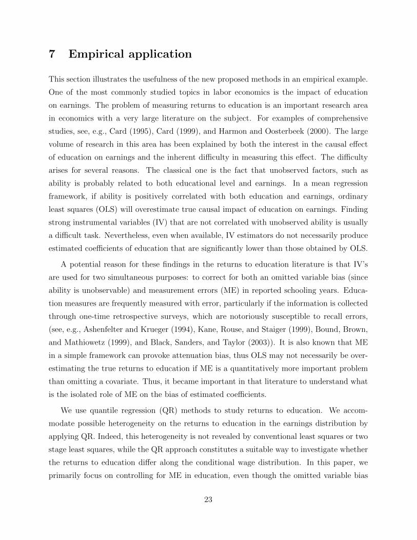
Figure 3 reports the QRME results after correcting for the ME problem. In general, the

estimates are smaller than those from QR and IV-QR. The QRME also presents a different

patten relative to the other estimates. The shape of the estimated coefficients for returns

to education looks very interesting. The QRME estimates exhibit a distinct inverted U-

shape, implying higher returns to schooling for those in the middle quantiles. In particular,

the QRME results show positive and monotonically-increasing returns to schooling at low

quantiles of the earnings distribution; estimated coefficient is increasing from 0.15 to 0.23

up to approximately 0.25 quantile. The returns start deceasing for higher quantiles. This

implies that the relative large wage gains from additional years of schooling accrue to those

at the lower end of the earnings distribution, and for high quantiles the returns of education

are smaller. The result can be, in part, associated with the fact that at the top of the

distribution of earnings, since individuals have high abilities, additional year of education

increases very little wages.

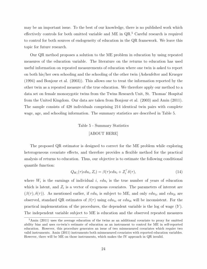
Figure 4 reports estimation results from QR based on a simple kernel density estimator

27

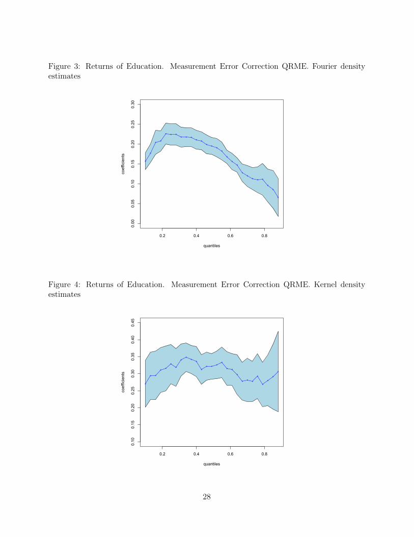
Figure 3: Returns of Education. Measurement Error Correction QRME. Fourier densityestimates

0.2 0.4 0.6 0.8

0.00

0.05

0.10

0.15

0.20

0.25

0.30

quantiles

coefficients

o

o

oo

o o oo o o

o o

oo

oo

o

o

o

oo

o o o

o

o

o

Figure 4: Returns of Education. Measurement Error Correction QRME. Kernel densityestimates

0.2 0.4 0.6 0.8

0.10

0.15

0.20

0.25

0.30

0.35

0.40

0.45

quantiles

coefficients

o

o o

oo

oo

oo

oo

oo o o

o

o o

o

o oo

o

o

o

o

o

28

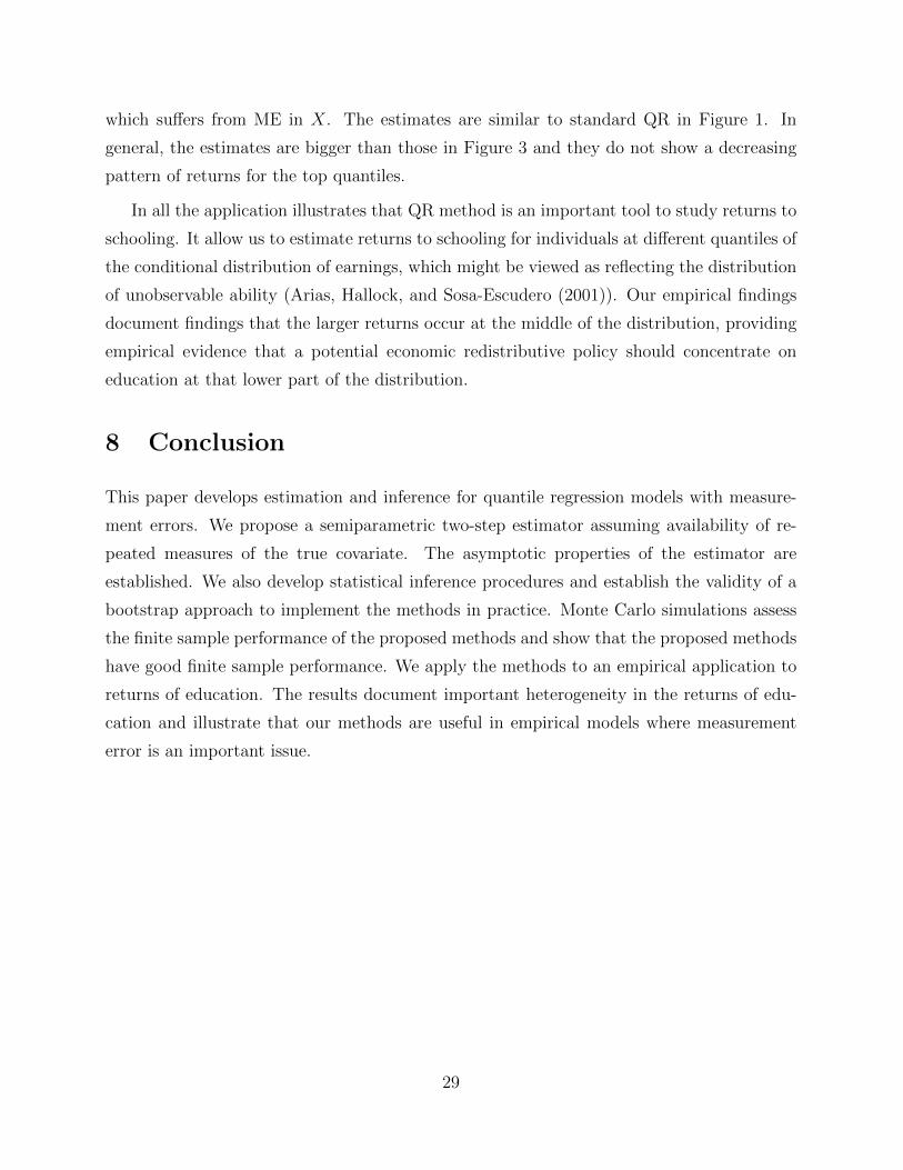
which suffers from ME in X. The estimates are similar to standard QR in Figure 1. In

general, the estimates are bigger than those in Figure 3 and they do not show a decreasing

pattern of returns for the top quantiles.

In all the application illustrates that QR method is an important tool to study returns to

schooling. It allow us to estimate returns to schooling for individuals at different quantiles of

the conditional distribution of earnings, which might be viewed as reflecting the distribution

of unobservable ability (Arias, Hallock, and Sosa-Escudero (2001)). Our empirical findings

document findings that the larger returns occur at the middle of the distribution, providing

empirical evidence that a potential economic redistributive policy should concentrate on

education at that lower part of the distribution.

8 Conclusion

This paper develops estimation and inference for quantile regression models with measure-

ment errors. We propose a semiparametric two-step estimator assuming availability of re-

peated measures of the true covariate. The asymptotic properties of the estimator are

established. We also develop statistical inference procedures and establish the validity of a

bootstrap approach to implement the methods in practice. Monte Carlo simulations assess

the finite sample performance of the proposed methods and show that the proposed methods

have good finite sample performance. We apply the methods to an empirical application to

returns of education. The results document important heterogeneity in the returns of edu-

cation and illustrate that our methods are useful in empirical models where measurement

error is an important issue.

29

A Mathematical Appendix

Proof of Theorem 1. Given Assumption A.III, we have

φ(ζ, y, z) ≡ E[eiζX | Y = y, Z = z]

=

∫E[eiζX | Y = y, Z = z,X = x]f(x | y, z)dx (15)

=

∫f(x | y, z)eiζxdx

(16)

where the last expression is the Fourier transform of f(x | y, z). Note that for (x, y, z) ∈ supp(X,Y, Z),

1

2π

∫φ(ζ, y, z) exp(−iζx)dζ

is the inverse Fourier transform of φ(ζ, y, z). Thus we have

f(x | y, z) =1

2π

∫φ(ζ, y, z) exp(−iζx)dζ.

We now need to show that

φ(ζ, Y, Z) =E[eiζX2 | Y,Z]

E[eiζX2 ]exp

(∫ ζ

0

iE[X1eiξX2 ]

E[eiξX2 ]dξ

).

From Assumptions A.I–II

Dξ ln(E[eiξX ]) =iE[XeiξX ]

E[eiξX ]

=iE[XeiξX ]E[eiξU2 ]

E[eiξX ]E[eiξU2 ]

=iE[Xeiξ(X+U2)]

E[eiξ(X+U2)]

=iE[Xeiξ(X+U2)] + iE[E(U1 | X,U2)eiξ(X+U2)]

E[eiξX2 ]

=iE[Xeiξ(X+U2)] + iE[E(U1e

iξ(X+U2) | X,U2)]

E[eiξX2 ]

=iE[Xeiξ(X+U2)] + iE[U1e

iξ(X+U2)]

E[eiξX2 ]

=iE[X1e

iξX2 ]

E[eiξX2 ].

30

Therefore, for each real ζ,

φ(ζ, Y, Z) ≡ E[eiζX | Y,Z]

=E[eiζX | Y, Z]E[eiζU2 ]

E[eiζX ]E[eiζU2 ]E[eiζX ]

=E[eiζX2 | Y, Z]

E[eiζX2 ]E[eiζX ]

=E[eiζX2 | Y, Z]

E[eiζX2 ]exp

(ln(E[eiζX ])− ln 1

)=

E[eiζX2 | Y, Z]

E[eiζX2 ]exp

(∫ ζ

0Dξ ln(E[eiξX ])dξ

)=

E[eiζX2 | Y,Z]

E[eiζX2 ]exp

(∫ ζ

0

iE[X1eiξX2 ]

E[eiξX2 ]dξ

),

where the third equality is obtained by U2 ⊥ (Y,X,Z).

Proof of Theorem 2. Note that the inverse Fourier Transform of κ(hxζ) is k(x/hx)/hx, andthe inverse Fourier Transform of E[eiζX | Y = y, Z = z] is f(x | y, z) by equation (13). Also notethat from the convolution theorem, the inverse Fourier Transform of the product of κ(hxζ) andE[eiζX | Y = y, Z = z] is the convolution between the inverse Fourier Transform of κ(hxζ) andthe inverse Fourier Transform of E[eiζX | Y = y, Z = z]. Because Assumptions A.II (iii)–A.IVguarantee the existence of f(x | y, z;hx), we conclude that

f(x | y, z;hx) ≡∫

1

hxk

(x− xhx

)f(x | y, z)dx

=1

2π

∫κ(hxζ)E[eiζX | Y = y, Z = z] exp(−iζx)dζ

=1

2π

∫κ(hxζ)φ(ζ, y, z) exp(−iζx)dζ.

The following lemma is helpful to derive the result given in Theorem 3.

Lemma A.1 For (x, y, z) ∈ supp(X,Y, Z) and hn > 0,

f(x | y, z;h)− f(x | y, z;h) = B(x, y, z;hx) + L(x, y, z;h) +R(x, y, z;h),

where B(x, y, z;hx) is a nonrandom “bias term” defined as

B(x, y, z;hx) ≡ f(x | y, z;hx)− f(x | y, z);

L(x, y, z;h) is a “variance term” admitting the linear representation

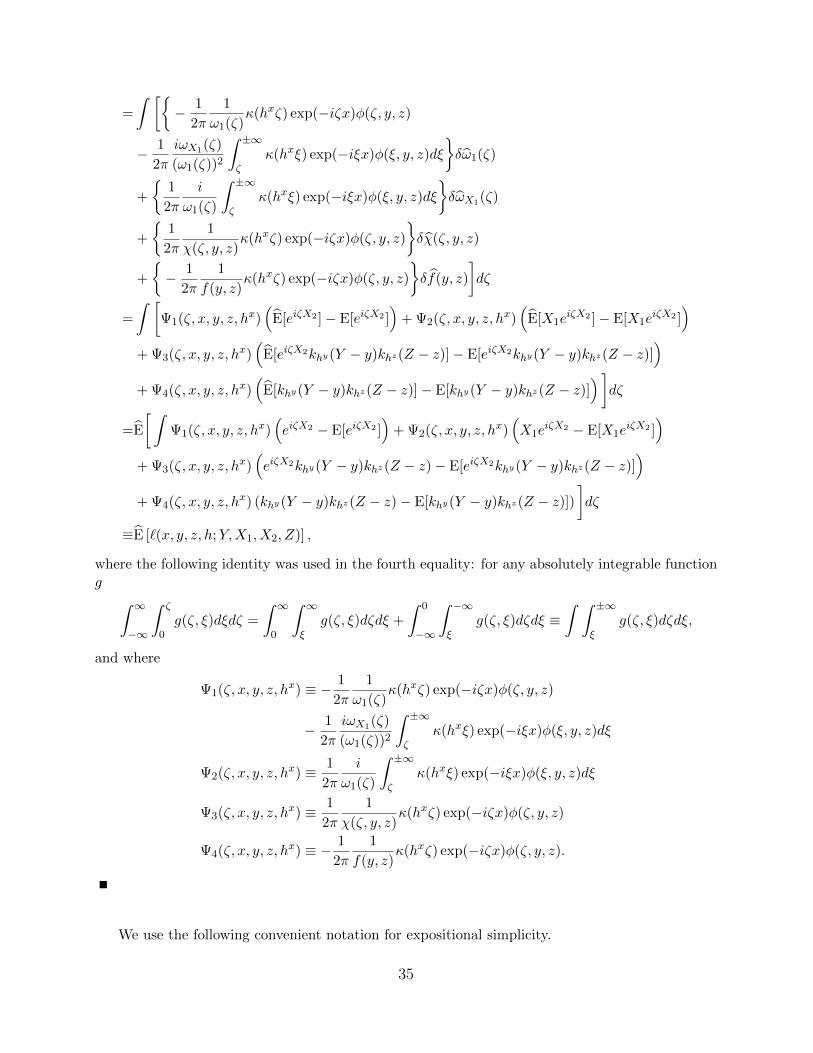
L(x, y, z;h) ≡ f(x | y, z;h)− f(x | y, z, hx) = E [`(x, y, z, h;Y,X1, X2, Z)]

31

where `(x, y, z, h;Y,X1, X2, Z) is defined in the proof of the lemma, and R(x, y, z;h) is a “remainderterm,”

R(x, y, z;h) ≡ f(x | y, z;h)− f(x | y, z;h).

Proof of Lemma A.1. Let ωA(ζ) ≡ E[AeiζX2

]where A = 1, X1 and

ω(ζ, y, x1, z) ≡ E[eiζX2 | Y = y, Z = z

]=

∫eiζx2f(x2 | y, z)dx2

=χ(ζ, y, z)

f(y, z),

where χ(ζ, y, z) ≡∫eiζx2f(x2, y, z)dx2. Also let ωA(ζ) ≡ E

[AeiζX2

]and δωA(ζ) ≡ ωA(ζ)− ωA(ζ),

and let

ω(ζ, y, z) ≡ E[eiζX2 | Y = y, Z = z

]≡ χ(ζ, y, z)/f(y, z)

where

χ(ζ, y, z) =1

n

n∑j=1

eiζX2jkhy(Yj − y)khz(Zj − z) = E[eiζX2khy(Y − y)khz(Z − z)

]f(y, z) =

1

n

n∑j=1

khy(Yj − y)khz(Zj − z) = E [khy(Y − y)khz(Z − z)] ,

and δχ(ζ, y, z) ≡ χ(ζ, y, z) − χ(ζ, y, z) and δf(y, z) ≡ f(y, z) − f(y, z). We use a following repre-sentation

ωX1(ζ)

ω1(ζ)=ωX1(ζ) + δωX1(ζ)

ω1(ζ) + δω1(ζ)= qX1(ζ) + δqX1(ζ) (17)

where qX1(ζ) = ωX1(ζ)/ω1(ζ) and where δqX1(ζ) can be written as either

δqX1(ζ) =

(δωX1(ζ)

ω1(ζ)− ωX1(ζ)δω1(ζ)

(ω1(ζ))2

)(1 +

δω1(ζ)

ω1(ζ)

)−1

or δqX1(ζ) = δ1qX1(ζ) + δ2qX1(ζ) with

δ1qX1(ζ) ≡ δωX1(ζ)

ω1(ζ)− ωX1(ζ)δω1(ζ)

(ω1(ζ))2

δ2qX1(ζ) ≡ ωX1(ζ)

ω1(ζ)

(δω1(ζ)

ω1(ζ)

)2(1 +

δω1(ζ)

ω1(ζ)

)−1

− δωX1(ζ)

ω1(ζ)

δω1(ζ)

ω1(ζ)

(1 +

δω1(ζ)

ω1(ζ)

)−1

.

Similarly,

1

ω1(ζ)=

1

ω1(ζ) + δω1(ζ)= q1(ζ) + δq1(ζ) (18)

32

where q1(ζ) ≡ 1/ω1(ζ), and where

δq1(ζ) =

(− δω1(ζ)

(ω1(ζ))2

)(1 +

δω1(ζ)

ω1(ζ)

)−1

or δq1(ζ) = δ1q1(ζ) + δ2q1(ζ) with

δ1q1(ζ) ≡ − δω1(ζ)

(ω1(ζ))2

δ2q1(ζ) ≡ 1

ω1(ζ)

(δω1(ζ)

ω1(ζ)

)2(1 +

δω1(ζ)

ω1(ζ)

)−1

.

And also

χ(ζ, y, z)

f(y, z)=χ(ζ, y, z) + δχ(ζ, y, z)

f(y, z) + δf(y, z)= q2(ζ, y, z) + δq2(ζ, y, z) (19)

where q2(ζ, y, z) ≡ χ(ζ, y, z)/f(y, z), and where

δq2(ζ, y, z) =

(δχ(ζ, y, z)

f(y, z)− χ(ζ, y, z)δf(y, z)

(f(y, z))2

)(1 +

δf(y, z)

f(y, z)

)−1

or δq2(ζ, y, z) = δ1q2(ζ, y, z) + δ2q2(ζ, y, z) with

δ1q2(ζ, y, z) ≡ δχ(ζ, y, z)

f(y, z)−χ(ζ, y, z)δf(y, z)

(f(y, z))2

δ2q2(ζ, y, z) ≡ χ(ζ, y, z)

f(y, z)

(δf(y, z)

f(y, z)

)2(1 +

δf(y, z)

f(y, z)

)−1

− δχ(ζ, y, z)

f(y, z)

δf(y, z)

f(y, z)

(1 +

δf(y, z)

f(y, z)

)−1

.

Let QX1(ζ) ≡∫ ζ

0 (iωX1(ξ)/ω1(ξ))dξ and δQX1(ζ) ≡∫ ζ

0 (iωX1(ξ)/ω1(ξ))dξ − QX1(ζ). Note that for

some random function δQX1(ζ) such that |δQX1(ζ)| ≤ |δQX1(ζ)| for all ζ,

exp(QX1(ζ) + δQX1(ζ)

)= exp(QX1(ζ))

(1 + δQX1(ζ) +

1

2

[exp(δQX1(ζ))

] (δQX1(ζ)

)2). (20)

33

From equations (14)∼(16), we have

f(x | y, z;h)− f(x | y, z;hx)

=1

2π

∫κ(hxζ)φ(ζ, y, z, h(2)) exp(−iζx)dζ − 1

2π

∫κ(hxζ)φ(ζ, y, z) exp(−iζx)dζ

=1

2π

∫κ(hxζ) exp(−iζx)

[ω(ζ, y, z)

ω1(ζ)exp

(∫ ζ

0

iωX1(ξ)

ω1(ξ)dξ

)− ω(ζ, y, z)

ω1(ζ)exp

(∫ ζ

0

iωX1(ξ)

ω1(ξ)dξ

)]dζ

=1

2π

∫κ(h1ζ) exp(−iζx)

[− ω(ζ, y, z)

ω1(ζ)exp

(∫ ζ

0

iωX1(ξ)

ω1(ξ)dξ

)+

χ(ζ, y, z)

f(y, z)+δχ(ζ, y, z)

f(y, z)− χ(ζ, y, z)δf(y, z)

(f(y, z))2+ δ2q2(ζ, y, z)

×

1

ω1(ζ)− δω1(ζ)

(ω1(ζ))2+ δ2q1(ζ)

× exp(QX1(ζ))

×

1 +

∫ ζ

0iδ1qX1(ξ)dξ +

∫ ζ

0iδ2qX1(ξ)dξ +

1

2exp(δQX1(ζ))

(∫ ζ

0iδqX1(ξ)dξ

)2]dζ.

We denote the linearization of f(x | y, z;hx) by f(x | y, z;hx). Then

L(x, y, z;h)

≡f(x | y, z;h)− f(x | y, z;hx)

=1

2π

∫κ(hxζ) exp(−iζx) exp(QX1(ζ))

[− χ(ζ, y, z)

f(y, z)

δω1(ζ)

(ω1(ζ))2

+χ(ζ, y, z)

f(y, z)

1

ω1(ζ)

∫ ζ

0iδ1qX1(ξ)dξ

+1

ω1(ζ)

δχ(ζ, y, z)

f(y, z)− 1

ω1(ζ)

χ(ζ, y, z)δf(y, z)

(f(y, z))2

]dζ

=1

2π

∫κ(hxζ) exp(−iζx)φ(ζ, y, z)

[− δω1(ζ)

ω1(ζ)+δχ(ζ, y, z)

χ(ζ, y, z)− δf(y, z)

f(y, z)

+

∫ ζ

0

(iδωX1(ξ)

ω1(ξ)− iωX1(ξ)δω1(ξ)

(ω1(ξ))2

)dξ

]dζ

=1

2π

∫κ(hxζ) exp(−iζx)φ(ζ, y, z)

(−δω1(ζ)

ω1(ζ)+δχ(ζ, y, z)

χ(ζ, y, z)− δf(y, z)

f(y, z)

)dζ

+1

2π

∫ ∫ ±∞ξ

κ(hxζ) exp(−iζx)φ(ζ, y, z)dζ

(iδωX1(ξ)

ω1(ξ)− iωX1(ξ)δω1(ξ)

(ω1(ξ))2

)dξ

=1

2π

∫κ(hxζ) exp(−iζx)φ(ζ, y, z)

(−δω1(ζ)

ω1(ζ)+δχ(ζ, y, z)

χ(ζ, y, z)− δf(y, z)

f(y, z)

)dζ

+1

2π

∫ ∫ ±∞ζ

κ(hxξ) exp(−iξx)φ(ξ, y, z)dξ

(iδωX1(ζ)

ω1(ζ)− iωX1(ζ)δω1(ζ)

(ω1(ζ))2

)dζ

34

=

∫ [− 1

2π

1

ω1(ζ)κ(hxζ) exp(−iζx)φ(ζ, y, z)

− 1

2π

iωX1(ζ)

(ω1(ζ))2

∫ ±∞ζ

κ(hxξ) exp(−iξx)φ(ξ, y, z)dξ

δω1(ζ)

+

1

2π

i

ω1(ζ)

∫ ±∞ζ

κ(hxξ) exp(−iξx)φ(ξ, y, z)dξ

δωX1(ζ)

+

1

2π

1

χ(ζ, y, z)κ(hxζ) exp(−iζx)φ(ζ, y, z)

δχ(ζ, y, z)

+

− 1

2π

1

f(y, z)κ(hxζ) exp(−iζx)φ(ζ, y, z)

δf(y, z)

]dζ

=

∫ [Ψ1(ζ, x, y, z, hx)

(E[eiζX2 ]− E[eiζX2 ]

)+ Ψ2(ζ, x, y, z, hx)

(E[X1e

iζX2 ]− E[X1eiζX2 ]

)+ Ψ3(ζ, x, y, z, hx)

(E[eiζX2khy(Y − y)khz(Z − z)]− E[eiζX2khy(Y − y)khz(Z − z)]

)+ Ψ4(ζ, x, y, z, hx)

(E[khy(Y − y)khz(Z − z)]− E[khy(Y − y)khz(Z − z)]

)]dζ

=E

[ ∫Ψ1(ζ, x, y, z, hx)

(eiζX2 − E[eiζX2 ]

)+ Ψ2(ζ, x, y, z, hx)

(X1e

iζX2 − E[X1eiζX2 ]

)+ Ψ3(ζ, x, y, z, hx)

(eiζX2khy(Y − y)khz(Z − z)− E[eiζX2khy(Y − y)khz(Z − z)]

)+ Ψ4(ζ, x, y, z, hx) (khy(Y − y)khz(Z − z)− E[khy(Y − y)khz(Z − z)])

]dζ

≡E [`(x, y, z, h;Y,X1, X2, Z)] ,

where the following identity was used in the fourth equality: for any absolutely integrable functiong ∫ ∞

−∞

∫ ζ

0g(ζ, ξ)dξdζ =

∫ ∞0

∫ ∞ξ

g(ζ, ξ)dζdξ +

∫ 0

−∞

∫ −∞ξ

g(ζ, ξ)dζdξ ≡∫ ∫ ±∞

ξg(ζ, ξ)dζdξ,

and where

Ψ1(ζ, x, y, z, hx) ≡ − 1

2π

1

ω1(ζ)κ(hxζ) exp(−iζx)φ(ζ, y, z)

− 1

2π

iωX1(ζ)

(ω1(ζ))2

∫ ±∞ζ

κ(hxξ) exp(−iξx)φ(ξ, y, z)dξ

Ψ2(ζ, x, y, z, hx) ≡ 1

2π

i

ω1(ζ)

∫ ±∞ζ

κ(hxξ) exp(−iξx)φ(ξ, y, z)dξ

Ψ3(ζ, x, y, z, hx) ≡ 1

2π

1

χ(ζ, y, z)κ(hxζ) exp(−iζx)φ(ζ, y, z)

Ψ4(ζ, x, y, z, hx) ≡ − 1

2π

1

f(y, z)κ(hxζ) exp(−iζx)φ(ζ, y, z).

We use the following convenient notation for expositional simplicity.

35

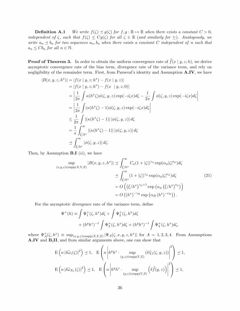
Definition A.1 We write f(ζ) g(ζ) for f, g : R 7→ R when there exists a constant C > 0,independent of ζ, such that f(ζ) ≤ Cg(ζ) for all ζ ∈ R (and similarly for ). Analogously, wewrite an bn for two sequences an, bn when there exists a constant C independent of n such thatan ≤ Cbn for all n ∈ N.

Proof of Theorem 3. In order to obtain the uniform convergence rate of f(x | y, z;h), we deriveasymptotic convergence rate of the bias term, divergence rate of the variance term, and rely onnegligibility of the remainder term. First, from Parseval’s identity and Assumption A.IV, we have

|B(x, y, z, hx)| = |f(x | y, z;hx)− f(x | y, z)|= |f(x | y, z;hx)− f(x | y, z; 0)|

=

∣∣∣∣ 1

2π

∫κ(hxζ)φ(ζ, y, z) exp(−iζx)dζ − 1

2π

∫φ(ζ, y, z) exp(−iζx)dζ

∣∣∣∣=

∣∣∣∣ 1

2π

∫(κ(hxζ)− 1)φ(ζ, y, z) exp(−iζx)dζ

∣∣∣∣≤ 1

2π

∫|(κ(hxζ)− 1)| |φ(ζ, y, z)| dζ

=1

π

∫ ∞ξ/hx|(κ(hxζ)− 1)| |φ(ζ, y, z)| dζ

∫ ∞ξ/hx|φ(ζ, y, z)| dζ.

Then, by Assumption B.I (ii), we have

sup(x,y,z)∈supp(X,Y,Z)

|B(x, y, z, hx)| ∫ ∞ξ/hx

Cφ(1 + |ζ|)γφ exp(αφ|ζ|νφ)dζ

∫ ∞ξ/hx

(1 + |ζ|)γφ exp(αφ|ζ|νφ)dζ (21)

= O((ξ/hx

)γφ+1exp

(αφ(ξ/hx

)νφ))= O

((hx)−γB exp

(αB (hx)−νB

)).

For the asymptotic divergence rate of the variance term, define

Ψ+(h) ≡∫

Ψ+1 (ζ, hx)dζ +

∫Ψ+

2 (ζ, hx)dζ

+ (hyhz)−1

∫Ψ+

3 (ζ, hx)dζ + (hyhz)−1

∫Ψ+

4 (ζ, hx)dζ,

where Ψ+A(ζ, hx) ≡ sup(x,y,z)∈supp(X,Y,Z) |ΨA(ζ, x, y, z, hx)| for A = 1, 2, 3, 4. From Assumptions

A.IV and B,II, and from similar arguments above, one can show that

E(n |δω1(ζ)|2

) 1, E

n ∣∣∣∣∣hyhz · sup(y,z)∈supp(Y,Z)

(δχ1(ζ, y, z))

∣∣∣∣∣2 1,

E(n |δωX1(ζ)|2

) 1, E

n ∣∣∣∣∣hyhz · sup(y,z)∈supp(Y,Z)

(δf(y, z)

)∣∣∣∣∣2 1,

36

and ∫Ψ+

1 (ζ, hx)dζ (1 + (hx)−1)γµ+γφ−γω+2 exp(−αω(hx)−1)νω

)exp

(αφ((hx)−1)νφ

),∫

Ψ+2 (ζ, hx)dζ (1 + (hx)−1)γφ−γω+2 exp

(−αω(hx)−1)νω

)exp

(αφ((hx)−1)νφ

),

(hyhz)−1

∫Ψ+

3 (ζ, hx)dζ (hyhz)−1(1 + (hx)−1)γφ−γω+1 exp(−αω(hx)−1)νω

)exp

(αφ((hx)−1)νφ

),

(hyhz)−1

∫Ψ+

4 (ζ, hx)dζ (hyhz)−1(1 + (hx)−1)γφ+1 exp(αφ((hx)−1)νφ

).

Then we have

Ψ+(h) = O(

max(1 + (hx)−1)γµ+1, (hyhz)−1(1 + (hx)−1

)γφ−γω+1exp

((αφ1νφ=νω − αω)((hx)−1)νω

)).

Note that by Minkowski inequality,

E

[sup

(x,y,z)∈supp(X,Y,Z)|L(x, y, z, h)|

]

= E

[sup

(x,y,z)∈supp(X,Y,Z)|f(x | y, z;h)− f(x | y, z;hx)|

]

= E

[sup

(x,y,z)∈supp(X,Y,Z)

∣∣∣∣ ∫ [Ψ1(ζ, x, y, z, hx)δω1(ζ) + Ψ2(ζ, x, y, z, hx)δωX1(ζ)

+ Ψ3(ζ, x, y, z, hx)δχ1(ζ, y, z) + Ψ4(ζ, x, y, z, hx)δf(y, z)]dζ

∣∣∣∣]≤ E

∫ [(sup

(x,y,z)∈supp(X,Y,Z)|Ψ1(ζ, x, y, z, hx)|

)|δω1(ζ)|

+

(sup

(x,y,z)∈supp(X,Y,Z)|Ψ2(ζ, x, y, z, hx)|

)|δωX1(ζ)|

+

(sup

(x,y,z)∈supp(X,Y,Z)|Ψ3(ζ, x, y, z, hx)|

)(sup

(y,z)∈supp(Y,Z)|δχ1(ζ, y, z)|

)

+

(sup

(x,y,z)∈supp(X,Y,Z)|Ψ4(ζ, x, y, z, hx)|

)(sup

(y,z)∈supp(Y,Z)

∣∣∣δf(y, z)∣∣∣) ]dζ

≤∫ [

Ψ+1 (ζ, hx)

E(|δω1(ζ)|2

)1/2+ Ψ+

2 (ζ, hx)

E(|δωX1(ζ)|2

)1/2

+ (hyhz)−1Ψ+3 (ζ, hx)

E

∣∣∣∣∣hyhz ·(

sup(y,z)∈supp(Y,Z)

δχ1(ζ, y, z)

)∣∣∣∣∣2

1/2

+ (hyhz)−1Ψ+4 (ζ, hx)

E

∣∣∣∣∣hyhz ·(

sup(y,z)∈supp(Y,Z)

δf(y, z)

)∣∣∣∣∣2

]dζ

37

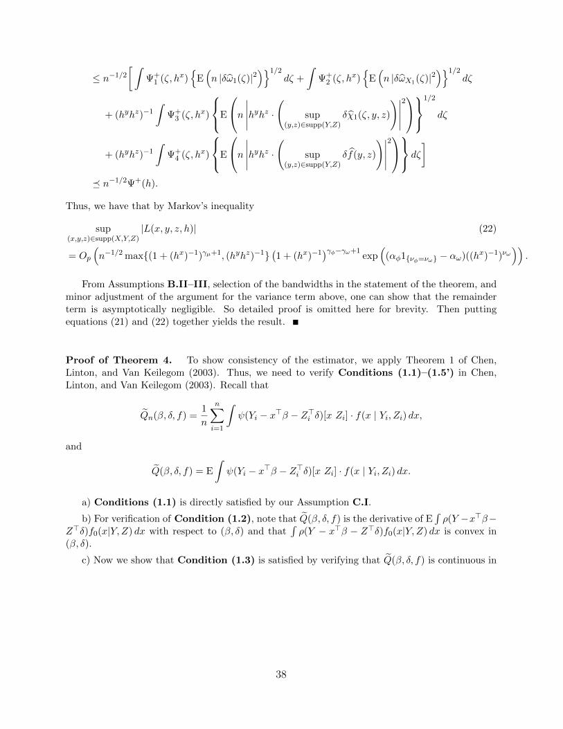
≤ n−1/2

[ ∫Ψ+

1 (ζ, hx)

E(n |δω1(ζ)|2

)1/2dζ +

∫Ψ+

2 (ζ, hx)

E(n |δωX1(ζ)|2

)1/2dζ

+ (hyhz)−1

∫Ψ+

3 (ζ, hx)

E

n ∣∣∣∣∣hyhz ·(

sup(y,z)∈supp(Y,Z)

δχ1(ζ, y, z)

)∣∣∣∣∣2

1/2

dζ

+ (hyhz)−1

∫Ψ+

4 (ζ, hx)

E

n ∣∣∣∣∣hyhz ·(

sup(y,z)∈supp(Y,Z)

δf(y, z)

)∣∣∣∣∣2 dζ

] n−1/2Ψ+(h).

Thus, we have that by Markov’s inequality

sup(x,y,z)∈supp(X,Y,Z)

|L(x, y, z, h)| (22)

= Op

(n−1/2 max(1 + (hx)−1)γµ+1, (hyhz)−1

(1 + (hx)−1

)γφ−γω+1exp

((αφ1νφ=νω − αω)((hx)−1)νω

)).

From Assumptions B.II–III, selection of the bandwidths in the statement of the theorem, andminor adjustment of the argument for the variance term above, one can show that the remainderterm is asymptotically negligible. So detailed proof is omitted here for brevity. Then puttingequations (21) and (22) together yields the result.

Proof of Theorem 4. To show consistency of the estimator, we apply Theorem 1 of Chen,Linton, and Van Keilegom (2003). Thus, we need to verify Conditions (1.1)–(1.5’) in Chen,Linton, and Van Keilegom (2003). Recall that

Qn(β, δ, f) =1

n

n∑i=1

∫ψ(Yi − x>β − Z>i δ)[x Zi] · f(x | Yi, Zi) dx,

and

Q(β, δ, f) = E

∫ψ(Yi − x>β − Z>i δ)[x Zi] · f(x | Yi, Zi) dx.

a) Conditions (1.1) is directly satisfied by our Assumption C.I.

b) For verification of Condition (1.2), note that Q(β, δ, f) is the derivative of E∫ρ(Y −x>β−

Z>δ)f0(x|Y,Z) dx with respect to (β, δ) and that∫ρ(Y − x>β − Z>δ)f0(x|Y,Z) dx is convex in

(β, δ).

c) Now we show that Condition (1.3) is satisfied by verifying that Q(β, δ, f) is continuous in

38

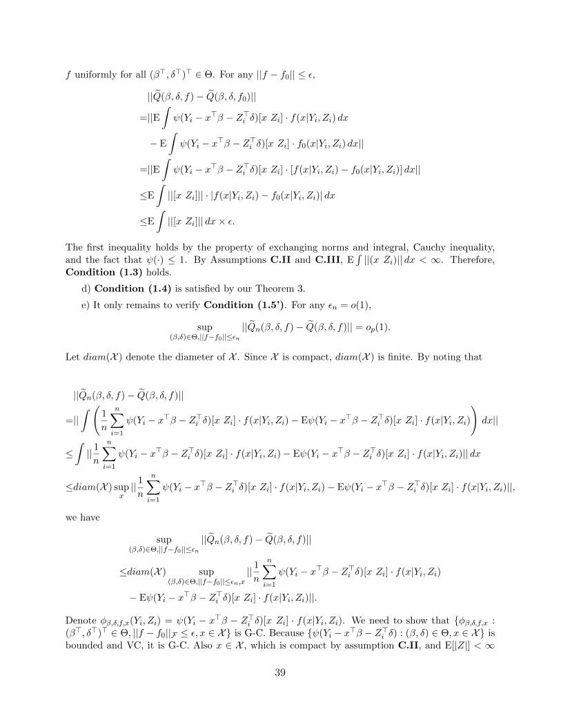
f uniformly for all (β>, δ>)> ∈ Θ. For any ||f − f0|| ≤ ε,

||Q(β, δ, f)− Q(β, δ, f0)||

=||E∫ψ(Yi − x>β − Z>i δ)[x Zi] · f(x|Yi, Zi) dx

− E

∫ψ(Yi − x>β − Z>i δ)[x Zi] · f0(x|Yi, Zi) dx||

=||E∫ψ(Yi − x>β − Z>i δ)[x Zi] · [f(x|Yi, Zi)− f0(x|Yi, Zi)] dx||

≤E

∫||[x Zi]|| · |f(x|Yi, Zi)− f0(x|Yi, Zi)| dx

≤E

∫||[x Zi]|| dx× ε.

The first inequality holds by the property of exchanging norms and integral, Cauchy inequality,and the fact that ψ(·) ≤ 1. By Assumptions C.II and C.III, E

∫||(x Zi)|| dx < ∞. Therefore,

Condition (1.3) holds.

d) Condition (1.4) is satisfied by our Theorem 3.

e) It only remains to verify Condition (1.5’). For any εn = o(1),

sup(β,δ)∈Θ,||f−f0||≤εn

||Qn(β, δ, f)− Q(β, δ, f)|| = op(1).

Let diam(X ) denote the diameter of X . Since X is compact, diam(X ) is finite. By noting that

||Qn(β, δ, f)− Q(β, δ, f)||

=||∫ (

1

n

n∑i=1

ψ(Yi − x>β − Z>i δ)[x Zi] · f(x|Yi, Zi)− Eψ(Yi − x>β − Z>i δ)[x Zi] · f(x|Yi, Zi)

)dx||

≤∫|| 1n

n∑i=1

ψ(Yi − x>β − Z>i δ)[x Zi] · f(x|Yi, Zi)− Eψ(Yi − x>β − Z>i δ)[x Zi] · f(x|Yi, Zi)|| dx

≤diam(X ) supx|| 1n

n∑i=1

ψ(Yi − x>β − Z>i δ)[x Zi] · f(x|Yi, Zi)− Eψ(Yi − x>β − Z>i δ)[x Zi] · f(x|Yi, Zi)||,

we have

sup(β,δ)∈Θ,||f−f0||≤εn

||Qn(β, δ, f)− Q(β, δ, f)||

≤diam(X ) sup(β,δ)∈Θ,||f−f0||≤εn,x

|| 1n

n∑i=1

ψ(Yi − x>β − Z>i δ)[x Zi] · f(x|Yi, Zi)

− Eψ(Yi − x>β − Z>i δ)[x Zi] · f(x|Yi, Zi)||.

Denote φβ,δ,f,x(Yi, Zi) = ψ(Yi − x>β − Z>i δ)[x Zi] · f(x|Yi, Zi). We need to show that φβ,δ,f,x :(β>, δ>)> ∈ Θ, ||f − f0||F ≤ ε, x ∈ X is G-C. Because ψ(Yi − x>β − Z>i δ) : (β, δ) ∈ Θ, x ∈ X isbounded and VC, it is G-C. Also x ∈ X , which is compact by assumption C.II, and E[|Z|] < ∞

39

by assumption C.III. Finally, Fεn = f : ||f − f0|| ≤ ε is G-C by Theorem 3. Those conditionsand Corollary 9.27 (ii) of Kosorok (2008) lead to our conclusion.

Proof of Theorem 5. We now apply Theorem 2 of Chen, Linton, and Van Keilegom (2003) toestablish weak convergence. We need to check their Conditions (2.1)–(2.6).

a) Condition (2.1) is satisfied by assumption G.I.

b) To verify Condition (2.2), note that

Q(β, δ, f0) = E

∫ψ(Yi − x>β − Z>i δ)[x Zi] · f0(x|Yi, Zi) dx

= EE[ψ(Yi − x>β − Z>i δ)[x Zi] · |Yi, Zi]= E[ψ(Yi − x>β − Z>i δ)[x Zi]]= EE[ψ(Y − x>β − Z>δ)[x Z]|X,Z]

= E[E[ψ(Y − x>β − Z>δ)|X,Z][x Z]]

= E[(τ −G(x>β + Z>δ))[x Z]].

The derivative with respect to (β, δ), denoted by Γ1(β, δ, f), is −Eg(x>β+Z>δ))[x Z][x Z]>. It iscontinuous in (β, δ) at (β0, δ0) and positive definite by Assumptions G.II and G.III.

c) Now we verify Condition (2.3). We first calculate the pathwise derivative of Q(β, δ, f) atf0:

Γ2(β, δ, f0)[f − f0] = [Q(β, δ, f0 + ζ(f − f0))− Q(β, δ, f0)]/ζ

=E

∫ψ(Yi − x>β − Z>i δ)[x Zi] · [f(x|Yi, Zi)− f0(x|Yi, Zi)] dx.

For any εn ↓ 0, such that ||(β, δ)− (β0, δ0)|| ≤ εn and ||f − f0|| ≤ εn:

||Q(β, δ, f)− Q(β, δ, f0)− Γ2(β, δ, f0)[f − f0]|| = 0

and

||Γ2(β, δ, f0)[f − f0]− Γ2(β0, δ0, f0)[f − f0]||

=||E∫

[ψ(Yi − x>β − Z>i δ)− ψ(Yi − x>β0 − Z>i δ0)][x Zi] · [f(x|Yi, Zi)− f0(x|Yi, Zi)] dx||

≤E

∫|ψ(Yi − x>β − Z>i δ)− ψ(Yi − x>β0 − Z>i δ0)| · ||[x Zi]|| dx× εn

=E

∫|1Yi − x>β − Z>i δ < 0 − 1Yi − x>β0 − Z>i δ0 < 0| · ||[x Zi]|| dx× εn

=o(1)× εn.

The inequality holds by the property of exchanging norm and integrals. The last equality holdsbecause the domain for integration is o(1) and X is compact.

d) Condition 2.4 holds by Assumption G.IV.

40

e) Now we verify Condition (2.5’):

sup||β−β0||≤εn,||δ−δ0||≤εn,||f−f0||≤εn

||Qn(β, δ, f)− Q(β, δ, f)− Qn(β0, δ0, f0)|| = op(1/√n)

Note that

||Qn(β, δ, f)− Q(β, δ, f)− Qn(β0, δ0, f0)||

=||∫ (

1

n

n∑i=1

ψ(Yi − x>β − Z>i δ)[x Zi] · f(x|Yi, Zi)− Eψ(Yi − x>β − Z>i δ)[x Zi] · f(x|Yi, Zi)

− 1

n

n∑i=1

ψ(Yi − x>β0 − Z>i δ0)[x Zi] · f0(x|Yi, Zi)

)− Eψ(Yi − x>β0 − Z>i δ0)[x Zi] · f0(x|Yi, Zi) dx||

≤∫|| 1n

n∑i=1

ψ(Yi − x>β − Z>i δ)[x Zi] · f(x|Yi, Zi)− Eψ(Yi − x>β − Z>i δ)[x Zi] · f(x|Yi, Zi)

− 1

n

n∑i=1

ψ(Yi − x>β0 − Z>i δ0)[x Zi] · f0(x|Yi, Zi)− Eψ(Yi − x>β0 − Z>i δ0)[x Zi] · f0(x|Yi, Zi)|| dx

≤diam(X ) supx|| 1n

n∑i=1

ψ(Yi − x>β − Z>i δ)[x Zi] · f(x|Yi, Zi)− Eψ(Yi − x>β − Z>i δ)[x Zi] · f(x|Yi, Zi)

− 1

n

n∑i=1

ψ(Yi − x>β0 − Z>i δ0)[x Zi] · f0(x|Yi, Zi)− Eψ(Yi − x>β0 − Z>i δ0)[x Zi] · f0(x|Yi, Zi)||.

So we need to show

sup||β−β0||≤εn,||δ−δ0||≤εn,||f−f0||≤εn,x

|| 1n

n∑i=1

ψ(Yi − x>β − Z>i δ)[x Zi] · f(x|Yi, Zi)

−Eψ(Yi − x>β − Z>i δ)[x Zi] · f(x|Yi, Zi)−1

n

n∑i=1

ψ(Yi − x>β0 − Z>i δ0)[x Zi] · f0(x|Yi, Zi)

+Eψ(Yi − x>β0 − Z>i δ0)[x Zi] · f0(x|Yi, Zi)|| = op(1/√n).

We need to show that φβ,δ,f,x is Donsker. Because ψ(Yi − x>β − Z>i δ) : (β, δ) ∈ Θ, x ∈ Xis bounded and VC, it is Donsker. Also x ∈ X , which is compact by Assumption C.II, andZ ∈ Z which is also compact by Assumption G.V. Finally, Fεn is uniformly bounded Donskerby Assumption G.VI. Those conditions and Corollary 9.32 (iii) of Kosorok (2008) lead to ourconclusion.

Finally, we verify Condition (2.6). Noting that√nQn(β0, δ0, f0) converges weakly and As-

sumption G.III, we only verify that

√nΓ2(β0, δ0, f0)[f − f0] =

√nE

∫ψ(Y − x>β0 − Z>δ0)[x Z] · (f(x|Y,Z)− f0(x|Y,Z)) dx

converges weakly. Also, since the bias of f is op(1/√n), we only need to verify

√nE∫ψ(Y −x>β0−

Zδ0)[x Z] · (f(x|Y,Z)− Ef(x|Y, Z)) dx converges weakly:

√nE

∫ψ(Y − x>β0 − Z>δ0)[x Z] · [ 1

2π

∫κ(hxnζ)(φ− Eφ)e−iζx dζ] dx. (23)

41

First,

supζ| 1n

n∑j=1

eiζX2j − EeiζX2j | p→ 0.

This is because eiζX2j = cos(ζX2j) + i sin(ζX2j) and those two terms are Lipschitz in ζ. Simi-

larly, 1n

∑nj=1X1e

iζX2jp→ EX1e

iζX2j . Therefore,1n

∑nj=1X1e

iζX2j

1n

∑nj=1 e

iζX2j

p→ EX1eiζX2j

EeiζX2j. By the continuous

mapping theorem,

exp

(∫ ζ

0

i 1n

∑nj=1X1e

iζX2j

1n

∑nj=1 e

iζX2j

)p→ exp

(∫ ζ

0

iEX1eiζX2j

EeiζX2j

)Also we have

E[eiζX2 | Y = y, Z = z] ≡1

hynhznn

∑[eiζX2khyn(Y − y)khzn(Z − z)]

1hynhznn

∑[khyn(Y − y)khzn(Z − z)]]

.

So (23) equals

√n

∫ ∫ψ(y − x>β0 − zδ0)[x z] · [ 1

2π

∫κ(hxnζ)(φ− φ)e−iζx dζ] dx dydz

=√n

∫ ∫ψ(y − x>β0 − zδ0)[x z] · [ 1

2π

∫κ(hxnζ)×

(1

hynhznn

∑[eiζX2khyn(Y − y)khzn(Z − z)]

exp

(∫ ζ

0

i 1n

∑nj=1X1e

iζX2j

1n

∑nj=1 e

iζX2j

)/

1

n

n∑j=1

eiζX2j1

hynhznn

∑[khyn(Y − y)khzn(Z − z)]− φ)

× e−iζx dζ] dx dydz

=√n

∫ ∫ψ(y − x>β0 − zδ0)[x z] · [ 1

2π

∫κ(hxnζ)(

1

hynhznn

∑[eiζX2khyn(Y − y)khzn(Z − z)]

[exp

(∫ ζ

0

iEX1eiζX2j

EeiζX2j

)+ op(1)]/[EeiζX2jf(y, z) + op(1)]− φ)e−iζx dζ] dx dydz

=√n 1

n

∑∫ψ(Yj − x>β0 − Zjδ0)[x Zj ] · [

1

2π

∫κ(hxnζ)×

[eiζX2j ][exp

(∫ ζ

0

iEX1eiζX2

EeiζX2

)+ op(1)]/[EeiζX2f(y, z) + op(1)]e−iζx dζ] dx− φ+ op(n

−1/2),

which converges weakly, and the result follows.

Proof of Lemma 1. The proof is a direct application of Theorem B in Chen, Linton, and VanKeilegom (2003) and parallel to that of weak convergence.

42

References

Amin, V. (2011): “Returns to Education: Evidence from UK Twins: Comment,” American Eco-nomic Review, 101, 1629–1635.

Arias, O., K. F. Hallock, and W. Sosa-Escudero (2001): “Individual Heterogeneity in theReturns to Schooling: Instrumental Variables Quantile Regression Using Twins Data,” EmpiricalEconomics, 26, 7–40.

Ashenfelter, O., and A. Krueger (1994): “Estimates of the Economic Return to Schoolingfrom a New Sample of Twins,” American Economic Review, 84, 1157–1173.

Black, D., S. Sanders, and L. Taylor (2003): “Measurement of Higher Education in theCensus and Current Population Survey,” Journal of the American Statistical Association, 98,545–554.

Bonjour, D., L. F. Cherkas, J. E. Haskel, D. D. Hawkes, and T. D. Spector (2003):“Returns to Education: Evidence from U.K. Twins,” American Economic Review, 93, 1799–1812.

Bound, J., C. Brown, and N. Mathiowetz (1999): “Measurement Error in Survey Data,” inHandbook of Econometrics, ed. by J. Heckman, and E. Leamer, vol. 5. North-Holland, Amster-dam.

Card, D. (1995): “Earnings, Schooling, and Ability Revisited,” in Research in Labor Economics,ed. by S. Polachek, vol. 14. JAI Press.

(1999): “The Causal Effect of Education on Earnings,” in Handbook of Labor Economics,ed. by O. Ashenfelter, and D. Card, vol. 3. Amsterdam: Elsevier.

Carroll, R. J., D. Ruppert, L. A. Stefanski, and C. M. Crainiceanu (2006): MeasurementError in Nonlinear Models. Chapman & Hall, Boca Raton, Florida.

Chen, X., O. Linton, and I. Van Keilegom (2003): “Estimation of Semiparametric ModelsWhen the Criterion Function is not Smooth,” Econometrica, 71, 1591–1608.

Chernozhukov, V., and C. Hansen (2005): “An IV Model of Quantile Treatment Effects,”Econometrica, 73, 245–261.

(2006): “Instrumental Quantile Regression Inference for Structural and Treatment EffectsModels,” Journal of Econometrics, 132, 491–525.

(2008): “Instrumental Variable Quantile Regression: A Robust Inference Approach,”Journal of Econometrics, 142, 379–398.

Chesher, A. (2001): “Parameter Approximations for Quantile Regressions with MeasurementError,” Working Paper CWP02/01, Department of Economics, University College London.

Delaigle, A., P. Hall, and A. Meister (2008): “On Deconvolution With Repeated Measure-ments,” The Annals of Statistics, 36, 665–685.

43

Fan, J. (1991a): “Asymptotic Normality for Deconvolution Kernel Density Estimators,” Sankhya: The Indian Journal of Statistics, Series A, 53, 97–110.

(1991b): “On the Optimal Rates of Convergence for Nonparametric Deconvolution Prob-lems,” The Annals of Statistics, 19, 1257–1272.

Fan, J., and Y. K. Truong (1993): “Nonparametric Regression with Errors in Variables,” TheAnnals of Statistics, 21, 1900–1925.

Galvao, A. F., and L. Wang (2015): “Uniformly Semiparametric Efficient Estimation of Treat-ment Effects with a Continuous Treatment,” Journal of the American Statistical Association,forthcoming.

Harmon, C. P., and H. Oosterbeek (2000): “The Returns to Education: A Review of theEvidence, Issues and Deficiencies in the Literature,” Centre for the Economics of Education,LSE.

Hausman, J., Y. Luo, and C. Palmer (2014): “Errors in the Dependent Variable of QuantileRegression Models,” Working Paper, MIT.

He, X., and H. Liang (2000): “Quantile Regression Estimates for a Class of Linear and PartiallyLinear Errors-in-Variables Models,” Statistica Sinica, 10, 129–140.

He, X., and Q.-M. Shao (1996): “A General Bahadur Representation of M-estimators andIts Application to Linear Regression with Nonstochastic Designs,” The Annals of Statistics, 6,2608–2630.

(2000): “On Parameters of Increasing Dimensions,” Journal of Multivariate Analysis, 73,120–135.

Hu, Y., and Y. Sasaki (2015): “Closed-form Estimation of Nonparametric Models with Non-classical Measurement Errors,” Journal of Econometrics, 185, 392–408.

Kane, T., C. Rouse, and D. Staiger (1999): “Estimating Returns to Schooling When Schoolingis Misreported,” NBER Working Papers No. 7235.

Koenker, R. (2005): Quantile Regression. Cambridge University Press, New York, New York.

Koenker, R., and G. W. Bassett (1978): “Regression Quantiles,” Econometrica, 46, 33–49.

Kosorok, M. (2008): Introduction to Empirical Processes and Semiparametric Inference. Springer.

Kotlarski, I. (1967): “On Characterizing the Gamma and the Normal Distribution,” PacificJournal of Mathematics, 20, 69–76.

Li, T. (2002): “Robust and Consistent Estimation of Nonlinear Errors-in-variables Models,” Jour-nal of Econometrics, 110, 1–26.

Li, T., and Q. Vuong (1998): “Nonparametric Estimation of the Measurement Error ModelUsing Multiple Indicators,” Journal of Multivariate Analysis, 65, 139–165.

44

Ma, Y., and G. Yin (2011): “Censored Quantile Regression with Covariate Measurement Errors,”Statistica Sinica, 21, 949–971.

Montes-Rojas, G. V. (2011): “Quantile Regression with Classical Additive Measurement Er-rors,” Economics Bulletin, 31, 2863–2868.

Newey, W. K., and D. L. McFadden (1994): “Large Sample Estimation and HypothesisTesting,” in Handbook of Econometrics, Vol. 4, ed. by R. F. Engle, and D. L. McFadden. NorthHolland, Elsevier, Amsterdam.

Pakes, A., and D. Pollard (1989): “Simulations and the Asymptotics of Optimization Estima-tors,” Econometrica, 57, 1027–1057.

Politis, D. N., and J. P. Romano (1999): “Multivariate Density Estimation with GeneralFlat-Top Kernels of Infinite Order,” Journal of Multivariate Analysis, 68, 1–25.

Powell, J. L. (1983): “The Asymptotic Normality of Two-Stage Least Absolute DeviationsEstimators,” Econometrica, 51, 1569–1575.

Schennach, S. M. (2004): “Estimation of Nonlinear Models with Measurement Error,” Econo-metrica, 72, 33–75.

(2007): “Instrumental Variable Estimation of Nonlinear Errors-in-Variables Models,”Econometrica, 75, 201–239.

(2008): “Quantile Regression with Mismeasured Covariates,” Econometric Theory, 24,1010–1043.

Torres-Saavedra, P. (2013): “Quantile Regression for Repeated Responses Measured with Er-ror,” North Carolina State University, mimeo.

Wang, H. J., L. A. Stefanski, and Z. Zhu (2012): “Corrected-Loss Estimation for QuantileRegression with Covariate Measurement Errors,” Biometrika, 99, 405–421.

Wei, Y., and R. J. Carroll (2009): “Quantile regression with measurement error,” Journal ofthe American Statistical Association, 104, 1129–1143.

Wu, Y., Y. Ma, and G. Yin (2014): “Smoothed and Corrected Score Approach to CensoredQuantile Regression With Measurement Errors,” Journal of the American Statistical Association,forthcoming.

45

Table 1: Fourier Estimatorhx\hy 0.2 0.3 0.4 0.5 0.6

B 0.09592 0.07751 0.09131 0.06610 0.093731.5 SD 0.09765 0.08403 0.11718 0.06085 0.08298

MSE 0.01874 0.01307 0.02207 0.00807 0.01567

B 0.09770 0.07553 0.08439 0.08457 0.096961.6 SD 0.09206 0.07425 0.08380 0.07819 0.07446

MSE 0.01802 0.01122 0.01414 0.01327 0.01495

B 0.10225 0.06963 0.07425 0.07394 0.099681.7 SD 0.10788 0.04347 0.09206 0.08228 0.08720

MSE 0.02209 0.00674 0.01399 0.01224 0.01754

B 0.09728 0.07464 0.07571 0.08745 0.104261.8 SD 0.08762 0.05453 0.06794 0.07288 0.07359

MSE 0.01714 0.00855 0.01035 0.01296 0.01629

B 0.08473 0.09663 0.08869 0.10269 0.104581.9 SD 0.02795 0.09039 0.08893 0.11265 0.08798

MSE 0.007961 0.017507 0.015774 0.023235 0.018679

optimal hx hy B SD MSE1.7 0.3 0.06963 0.04347 0.00674

46

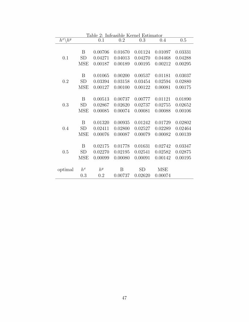
Table 2: Infeasible Kernel Estimatorhx\hy 0.1 0.2 0.3 0.4 0.5

B 0.00706 0.01670 0.01124 0.01097 0.033310.1 SD 0.04271 0.04013 0.04270 0.04468 0.04288

MSE 0.00187 0.00189 0.00195 0.00212 0.00295

B 0.01065 0.00200 0.00537 0.01181 0.030370.2 SD 0.03394 0.03158 0.03454 0.02594 0.02880

MSE 0.00127 0.00100 0.00122 0.00081 0.00175

B 0.00513 0.00737 0.00777 0.01121 0.018900.3 SD 0.02867 0.02620 0.02737 0.02755 0.02652

MSE 0.00085 0.00074 0.00081 0.00088 0.00106

B 0.01320 0.00935 0.01242 0.01729 0.028020.4 SD 0.02411 0.02800 0.02527 0.02289 0.02464

MSE 0.00076 0.00087 0.00079 0.00082 0.00139

B 0.02175 0.01778 0.01631 0.02742 0.033470.5 SD 0.02270 0.02195 0.02541 0.02582 0.02875

MSE 0.00099 0.00080 0.00091 0.00142 0.00195

optimal hx hy B SD MSE0.3 0.2 0.00737 0.02620 0.00074

47

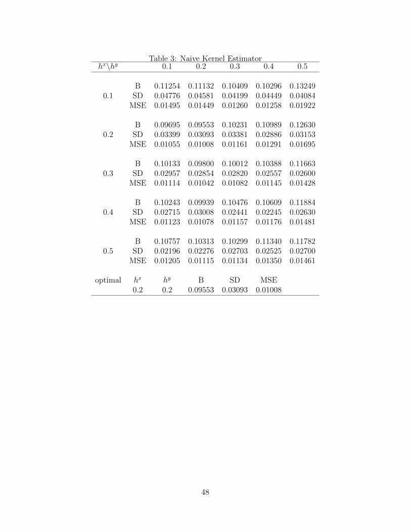
Table 3: Naive Kernel Estimatorhx\hy 0.1 0.2 0.3 0.4 0.5

B 0.11254 0.11132 0.10409 0.10296 0.132490.1 SD 0.04776 0.04581 0.04199 0.04449 0.04084

MSE 0.01495 0.01449 0.01260 0.01258 0.01922

B 0.09695 0.09553 0.10231 0.10989 0.126300.2 SD 0.03399 0.03093 0.03381 0.02886 0.03153

MSE 0.01055 0.01008 0.01161 0.01291 0.01695

B 0.10133 0.09800 0.10012 0.10388 0.116630.3 SD 0.02957 0.02854 0.02820 0.02557 0.02600

MSE 0.01114 0.01042 0.01082 0.01145 0.01428

B 0.10243 0.09939 0.10476 0.10609 0.118840.4 SD 0.02715 0.03008 0.02441 0.02245 0.02630

MSE 0.01123 0.01078 0.01157 0.01176 0.01481

B 0.10757 0.10313 0.10299 0.11340 0.117820.5 SD 0.02196 0.02276 0.02703 0.02525 0.02700

MSE 0.01205 0.01115 0.01134 0.01350 0.01461

optimal hx hy B SD MSE0.2 0.2 0.09553 0.03093 0.01008

48

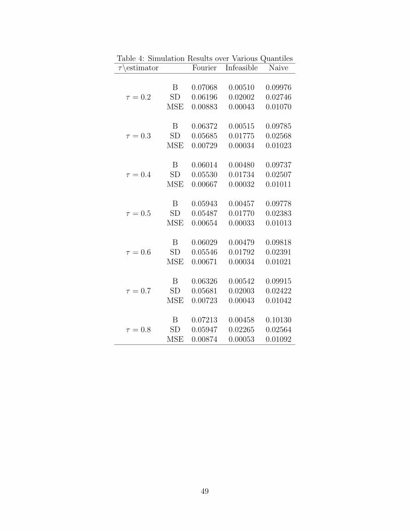
Table 4: Simulation Results over Various Quantilesτ\estimator Fourier Infeasible Naive

B 0.07068 0.00510 0.09976τ = 0.2 SD 0.06196 0.02002 0.02746

MSE 0.00883 0.00043 0.01070

B 0.06372 0.00515 0.09785τ = 0.3 SD 0.05685 0.01775 0.02568

MSE 0.00729 0.00034 0.01023

B 0.06014 0.00480 0.09737τ = 0.4 SD 0.05530 0.01734 0.02507

MSE 0.00667 0.00032 0.01011

B 0.05943 0.00457 0.09778τ = 0.5 SD 0.05487 0.01770 0.02383

MSE 0.00654 0.00033 0.01013

B 0.06029 0.00479 0.09818τ = 0.6 SD 0.05546 0.01792 0.02391

MSE 0.00671 0.00034 0.01021

B 0.06326 0.00542 0.09915τ = 0.7 SD 0.05681 0.02003 0.02422

MSE 0.00723 0.00043 0.01042

B 0.07213 0.00458 0.10130τ = 0.8 SD 0.05947 0.02265 0.02564

MSE 0.00874 0.00053 0.01092

49

Table 5: Summary StatisticsMEAN S.D. MIN MAX

Log of Wage 2.117 0.571 -1.426 4.573Education (self-report) 14.110 2.501 10.000 17.000

Education (twin’s report) 13.925 2.526 10.000 17.000Age 42.477 10.050 21.000 59.000

Number of observations 428

50