Edinburgh Research Explorer

CAPRI: efficient inference of cancer progression models fromcross-sectional data

Citation for published version:Ramazzotti, D, Caravagna, G, Olde Loohuis, L, Graudenzi, A, Korsunsky, I, Mauri, G, Antoniotti, M &Mishra, B 2015, 'CAPRI: efficient inference of cancer progression models from cross-sectional data'Bioinformatics, vol. 31, no. 18, pp. 3016-26. DOI: 10.1093/bioinformatics/btv296

Digital Object Identifier (DOI):10.1093/bioinformatics/btv296

Link:Link to publication record in Edinburgh Research Explorer

Document Version:Peer reviewed version

Published In:Bioinformatics

General rightsCopyright for the publications made accessible via the Edinburgh Research Explorer is retained by the author(s)and / or other copyright owners and it is a condition of accessing these publications that users recognise andabide by the legal requirements associated with these rights.

Take down policyThe University of Edinburgh has made every reasonable effort to ensure that Edinburgh Research Explorercontent complies with UK legislation. If you believe that the public display of this file breaches copyright pleasecontact openaccess@ed.ac.uk providing details, and we will remove access to the work immediately andinvestigate your claim.

Download date: 22. Feb. 2019

CAPRI: Efficient Inference of Cancer Progression

Models from Cross-sectional Data

Daniele Ramazzotti ∗† Giulio Caravagna † Loes Olde Loohuis ‡

Alex Graudenzi † Ilya Korsunsky § Giancarlo Mauri †

Marco Antoniotti † Bud Mishra §

Abstract

We devise a novel inference algorithm to effectively solve the cancer pro-gression model reconstruction problem. Our empirical analysis of the ac-curacy and convergence rate of our algorithm, CAncer PRogression Infer-ence (CAPRI), shows that it outperforms the state-of-the-art algorithmsaddressing similar problems.

Motivation: Several cancer-related genomic data have become avail-able (e.g., The Cancer Genome Atlas, TCGA) typically involving hun-dreds of patients. At present, most of these data are aggregated in across-sectional fashion providing all measurements at the time of diagno-sis.

Our goal is to infer cancer “progression” models from such data. Thesemodels are represented as directed acyclic graphs (DAGs) of collectionsof “selectivity” relations, where a mutation in a gene A “selects” for alater mutation in a gene B. Gaining insight into the structure of suchprogressions has the potential to improve both the stratification of patientsand personalized therapy choices.

Results: The CAPRI algorithm relies on a scoring method based on aprobabilistic theory developed by Suppes, coupled with bootstrap and max-imum likelihood inference. The resulting algorithm is efficient, achieveshigh accuracy, and has good complexity, also, in terms of convergenceproperties. CAPRI performs especially well in the presence of noise inthe data, and with limited sample sizes. Moreover CAPRI, in contrast toother approaches, robustly reconstructs different types of confluent tra-jectories despite irregularities in the data.

∗To whom correspondence should be addressed.†Deptartment of Informatics, Systems and Communication, University of Milan Bicocca,

Milan, Italy.‡Center for Neurobehavioral Genetics, University of California Los Angeles, Los Angeles,

USA.§Courant Institute of Mathematical Sciences, New York University, New York, USA

1

We also report on an ongoing investigation using CAPRI to studyatypical Chronic Myeloid Leukemia, in which we uncovered non trivialselectivity relations and exclusivity patterns among key genomic events.

Availability: CAPRI is part of the TRanslational ONCOlogy R pack-age and is freely available on the web at:http://bimib.disco.unimib.it/index.php/Tronco

Contact: daniele.ramazzotti@disco.unimib.it

1 Introduction

Analysis and interpretation of the fast-growing biological data sets that arecurrently being curated from laboratories all over the world require sophisticatedcomputational and statistical methods.

Motivated by the availability of genetic patient data, we focus on the problemof reconstructing progression models of cancer. In particular, we aim to infer theplausible sequences of genomic alterations that, by a process of accumulation,selectively make a tumor fitter to survive, expand and diffuse (i.e., metastasize).Along the trajectories of progression, a tumor (monotonically) acquires or “ac-tivates” mutations in the genome, which, in turn, produce progressively more“viable” clonal subpopulations over the so-called cancer evolutionary landscape(cfr., [23, 33,49]).

Knowledge of such progression models is very important for drug develop-ment and in therapeutic decisions. For example, it has been known that for thesame cancer type, patients in different stages of different progressions responddifferently to different treatments.

Several datasets are currently available that aggregate diverse cancer-patientdata and report in-depth mutational profiles, including e.g., structural changes(e.g., inversions, translocations, copy-number variations) or somatic mutations(e.g., point mutations, insertions, deletions, etc.). An example of such a datasetis The Cancer Genome Atlas (TCGA) (cfr., [36])). These data, by their verynature, only give a snapshot of a given tumor sample, mostly from biopsies ofuntreated tumor samples at the time of diagnoses. It still remains impracticalto track the tumor progression in any single patient over time, thus limitingmost analysis methods to work with cross-sectional data1.

To rephrase, we focus on the problem of cancer progression models recon-struction from cross-sectional data. The problem is not new and, to the best ofour knowledge, two threads of research starting in the late 90’s have addressed it.The first category of works examined mostly gene-expression data to reconstructthe temporal ordering of samples (cfr., [16, 31]). The second category of workslooked at inferring cancer progression models of increasing model-complexity,starting from the simplest tree models (cfr. [9]) to more complex graph models

1Unlike longitudinal studies, these cross-sectional data are derived from samples that arecollected at unknown time points, and can be considered as “static”.

2

Figure 1: Selectivity Relation in Tumor Evolution. The CAncer PRogres-sion Inference (CAPRI) algorithm examines cancer patients’ genomic cross-sectional data to determine relationships among genomic alterations (e.g., so-matic mutations, copy-number variations, etc.) that modulate the somatic evo-lution of a tumor. When CAPRI concludes that aberration a (say, an egfrmutation) “selects for” aberration b (say, a cdk mutation), such relations canbe rigorously expressed using Suppes’ conditions, which postulates that if a se-lects b, then a occurs before b (temporal priority) and occurrences of a raises theprobability of emergence of b (probability raising). Moreover, CAPRI is capableof reconstructing relations among more complex boolean combination of events,as shown in the bottom panel and discussed in the Approach section.

(cfr., [15]); see the next subsection for an overview of the state of the art. Build-ing on our previous work described in [37] we present a novel and comprehensivealgorithm of the second category that addresses this problem.

The new algorithm proposed here is called CAncer PRogression Inference(CAPRI) and is part of the TRanslational ONCOlogy (TRONCO) package(cfr., [2]). Starting from cross-sectional genomic data, CAPRI reconstructs aprobabilistic progression model by inferring “selectivity relations”, where a mu-tation in a gene A “selects” for a later mutation in a gene B. These relations aredepicted in a combinatorial graph and resemble the way a mutation exploits its“selective advantage” to allow its host cells to expand clonally. Among otherthings, a selectivity relation implies a putatively invariant temporal structureamong the genomic alterations (i.e., events) in a specific cancer type. In addi-tion, these relations are expected to also imply “probability raising” for a pairof events in the following sense: Namely, a selectivity relation between a pairof events here signifies that the presence of the earlier genomic alteration (i.e.,the upstream event) that is advantageous in a Darwinian competition scenarioincreases the probability with which a subsequent advantageous genomic alter-ation (i.e., the downstream event) appears in the clonal evolution of the tumor.Thus the selectivity relation captures the effects of the evolutionary processes,

3

and not just correlations among the events and imputed clocks associated withthem. As an example, we show in (Figure 1) the selectivity relation connectinga mutation of egfr to the mutation of cdk.

Consequently, an inferred selectivity relation suggests mutational profilesin which certain samples (early-stage patients) display specific alterations only(e.g., the alteration characterizing the beginning of the progression), while cer-tain other samples (e.g., late-stage patients) display a superset subsuming theearly mutations (as well as alterations that occur subsequently in the progres-sion).

Various kinds of genomic aberrations are suitable as input data, and in-clude somatic point/indel mutations, copy-number alterations, etc., providedthat they are persistent, i.e., once an alteration is acquired no other genomicevent can restore the cell to the non-mutated (i.e., wild type) condition2.

The selectivity relations that CAPRI reconstructs are ranked and subse-quently further refined by means of a hybrid algorithm, which reasons over time,mechanism and chance, as follows. CAPRI’s overall scoring methods combinetopological constraints grounded on Patrick Suppes’ conditions of probabilis-tic causation (see e.g., [44]), with a maximum likelihood-fit procedure (cfr., [28])and derives much of its statistical power from the application of bootstrap proce-dures (see e.g., [11]). CAPRI returns a graphical model of a complex selectivityrelation among events which captures the essential aspects of cancer evolution:branches, confluences and independent progressions. In the specific case ofconfluences, CAPRI’s ability to infer them is related to the complexity of the“patterns” they exhibit, expressed in a logical fashion. As pointed out by otherapproaches (cfr., [4]), this strategy requires trading off complexity for expressiv-ity of the inferred models, and results in two execution modes for the algorithm:supervised and unsupervised, which we discuss in details in Sections 2 and 3.

In Section 3 (Methods) we show that CAPRI enjoys a set of attractive prop-erties in terms of its complexity, soundness and expressivity, even in the presenceof uniform noise in the input data – e.g., due to genetic heterogeneity and ex-perimental errors. Although many other approaches enjoy similar asymptoticproperties, we show that CAPRI can compute accurate results with surpris-ingly small sample sizes (cfr., Section 4). Moreover, to the best of our knowl-edge, based on extensive synthetic data simulations, CAPRI outperforms allthe competing procedures with respect to all desirable performance metrics.We conclude by showing an application of CAPRI to reconstruct a progressionmodel for atypical Chronic Myeloid Leukemia (aCML) using a recent exomesequencing dataset, first presented in [41].

2For instance, epigenetic alterations such as methylation and alterations in gene expressionare not directly usable as input data for the algorithm. Notice that the selection of the relevantevents is beyond the scope of this work and requires a further upstream pipeline, such as thatprovided, for instance, in [46,49].

4

1.1 State of the Art

For an extensive review on cancer progression model reconstruction we referto the recent survey by [6]. In brief, progression models for cancer have beenstudied starting with the seminal work of [48] where, for the first time, cancerprogression was described in terms of a directed path by assuming the existenceof a unique and most likely temporal order of genetic mutations. [48] manuallycreated a (colorectal) cancer progression from a genetic and clinical point ofview. More rigorous and complex algorithmic and statistical automated ap-proaches have appeared subsequently. As stated already, the earliest thread ofresearch simply sought more generic progression models that could assume tree-like structures. The oncogenetic tree model captured evolutionary branches ofmutations (cfr., [9, 45]) by optimizing a correlation-based score. Another pop-ular approach to reconstruct tree structures appears in [10]. Other generalMarkov chain models such as, e.g., [21] reconstruct more flexible probabilisticnetworks, despite a computationally expensive parameter estimation. In [37],we introduced an algorithm called CAncer PRogression Extraction with SingleEdges (CAPRESE), which, based on its extensive empirical analysis, may bedeemed as the current state-of-the-art algorithm for the inference of tree mod-els of cancer progression. It is based on a shrinkage-like statistical estimation,grounded in a general theoretical framework, which we extend further in thispaper. Other results that extend tree representations of cancer evolution exploitmixture tree models, i.e., multiple oncogenetic trees, each of which can indepen-dently result in cancer development (cfr., [5]). In general, all these methods arecapable of modeling diverging temporal orderings of events in terms of branches,although the possibility of converging evolutionary paths is precluded.

To overcome this limitation, the most recent approaches tends to adoptBayesian graphical models, i.e., Bayesian Networks (BN). In the literature, therehave been two initial families of methods aimed at inferring the structure of aBN from data (cfr., [28]). The first class of models seeks to explicitly capture allthe conditional independence relations encoded in the edges and will be referredto as structural approaches; the methods in this family are inspired by the workon causal theories by Judea Pearl (cfr., [39, 40, 43, 47]). The second class –likelihood approaches – seeks a model that maximizes the likelihood of the data(cfr., [7, 19,42]).

A more recent hybrid approach to learn a BN which combines the two fam-ilies above by (i) constraining the search space of the valid solutions and, then,(ii) fitting the model with likelihood maximization (see [4, 15, 34]). A furthertechnique to reconstruct progression models from cross-sectional data was in-troduced in [3], in which the transition probabilities between genotypes areinferred by defining a Moran process that describes the evolutionary dynamicsof mutation accumulation. In [8] this methodology was extended to account forpathway-based phenotypic alterations.

5

2 Approach

In what follows, we denote with P(·) and P(· | ·) the observed marginal andconditional probability of an event, whose complement is denoted with the di-acritical mark · (macron).

A probabilistic model of selective advantage. Central to CAPRI’s scorefunction is Suppes’ notion of probabilistic causation (cfr., [44]), which can bestated in the following terms: a selectivity relation3 among two observables i andj if (1) i occurs earlier than j – temporal priority (tp) – and (2) if the probabilityof observing i raises the probability of observing j, i.e., P(j | i) > P(j | i) –probability raising (pr). The definition of probability raising subsumes positivestatistical dependency and mutuality (see, e.g., [37]). Note that the resultingrelation (also, called prima facie causality) is purely observational and remainsagnostic to the possible mechanistic cause-effect relation involving i and j.

While Suppes’ definition of probabilistic causation has known limitationsin the context of general causality theory (see discussions in, e.g., [20, 26]), inthe context of cancer evolution, this relation appropriately describes variousfeatures of selective advantage in somatic alterations that accumulate as tumorprogresses.

Thus, in our framework, we implement the temporal priority among events– condition (1) – as P(i) > P(j), because it is intuitively sound to assumethat the (cumulative) genomic events occurring earlier are the ones present inhigher frequency in a dataset. In addition, condition (2) is implemented as is,that is by requiring that for each pair of observables i and j directly connected,P(j | i) > P(j | i) is verified. Taken together, these conditions gives rise to anatural ordering relation among events, written “i B j” and read as “i has aselective influence on j.” This relation is a necessary but not sufficient conditionto capture the notion of selective advantage, and additional constraints need tobe imposed to filter spurious relations. Spurious correlations are both intrinsicto the definition (e.g., if iB jBw then also iBw, which could be spurious) andto the model we aim at inferring, because data is finite as well as corrupted bynoise.

Building on this framework, we devise inference algorithms that capture theessential aspects of heterogeneous cancer progressions: branching, independenceand convergence – all combining in a progression model.

Progression patterns. The complexity of cancer requires modeling multiplenon-trivial patterns of its progression: for a specific event, a pattern is definedas a specific combination of the closest upstream events that confers a selectiveadvantage.

As an example, imagine a clonal subpopulation becoming fit – thus enjoyingexpansion and selection – once it acquires a mutation of gene c, provided it also

3Suppes presents the relation in terms of causality; however, we avoid Suppes’ terminologyas we build on just two of his many axioms, which only give rise to the notion of prima-faciecausality.

6

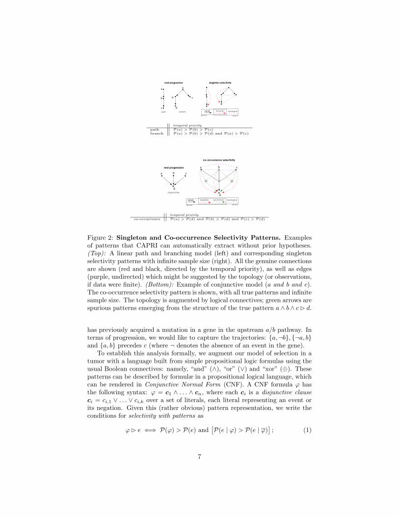
singleton selectivityreal progression

path branch

a

b

c

a

b c

dreal transitivity topological

genuine spurious

temporal priority

path P(a) > P(b) > P(c)branch P(a) > P(b) > P(d) and P(a) > P(c)

co-occurrence selectivity

∧ ∧ ∧

real progression a b c

a b c

conjunctive

real transitivity sub-formula

genuine spurious

topological

d

d

temporal priority

co-occurrence P(a) > P(d) and P(b) > P(d) and P(c) > P(d)

Figure 2: Singleton and Co-occurrence Selectivity Patterns. Examplesof patterns that CAPRI can automatically extract without prior hypotheses.(Top): A linear path and branching model (left) and corresponding singletonselectivity patterns with infinite sample size (right). All the genuine connectionsare shown (red and black, directed by the temporal priority), as well as edges(purple, undirected) which might be suggested by the topology (or observations,if data were finite). (Bottom): Example of conjunctive model (a and b and c).The co-occurrence selectivity pattern is shown, with all true patterns and infinitesample size. The topology is augmented by logical connectives; green arrows arespurious patterns emerging from the structure of the true pattern a ∧ b ∧ cB d.

has previously acquired a mutation in a gene in the upstream a/b pathway. Interms of progression, we would like to capture the trajectories: {a,¬b}, {¬a, b}and {a, b} precedes c (where ¬ denotes the absence of an event in the gene).

To establish this analysis formally, we augment our model of selection in atumor with a language built from simple propositional logic formulas using theusual Boolean connectives: namely, “and” (∧), “or” (∨) and “xor” (⊕). Thesepatterns can be described by formulæ in a propositional logical language, whichcan be rendered in Conjunctive Normal Form (CNF). A CNF formula ϕ hasthe following syntax: ϕ = c1 ∧ . . . ∧ cn, where each ci is a disjunctive clauseci = ci,1 ∨ . . . ∨ ci,k over a set of literals, each literal representing an event orits negation. Given this (rather obvious) pattern representation, we write theconditions for selectivity with patterns as

ϕB e ⇐⇒ P(ϕ) > P(e) and[P(e | ϕ) > P(e | ϕ)

]; (1)

7

with respect to the example above, patterns 4 could be a ∨ bB c and a⊕ bB cIn our framework the problem of reconstructing a probabilistic graphical

model of progression reduces to the following: for each input event e, assess a setof selectivity patterns {ϕ1 Be, . . . , ϕkBe}, filter the spurious ones, and combinethe rest in a direct acyclic graph (DAG)5, augmented with logical symbols.Notice that while we broke down the progression extraction into a series ofsub-tasks, the problem remains complex: patterns are unknown, potentiallyspurious, and exponential in formula size; data is noisy; patterns must allowfor “imperfect regularities”, rather than being strict6. To summarize, in oursetting we can model complex progression trajectories with branches (i.e., eventsinvolved in various patterns), independent progressions (i.e., events withoutcommon ancestors) and convergence (via CNF formulas). The framework weintroduce here is highly versatile, and to the best of our knowledge, it infers andchecks more complex claims than any cancer progression algorithms describedthus far (cfr., [9, 15,37]).

3 Methods

Building on the framework described in the previous section, we now describe theimplementation of CAPRI’s building blocks. Notice that, in general, the infer-ence of cancer progression models requires a complex data processing pipeline, assummarized in Figure 3; its architecture optimally exploits CAPRI’s efficiency.

Assumptions. CAPRI relies on the following assumptions: i) Every patternis expressible as a propositional CNF formula; ii) All events are persistent, i.e.,an acquired mutation cannot disappear; iii) All relevant events in tumor pro-gression are observable, with the observations describing the progressive phe-nomenon in an essential manner (i.e., closed world assumption, in which allevents ‘driving’ the progression are detectable); iv) All the events have non-degenerate observed probability in (0, 1); v) All events are distinguishable, inthe following sense: input alterations produce different profiles across inputsamples. Assumptions i-ii) relate to the framework derived in previous sec-tion, while iii) imposes an onerous burden on the experimentalists, who mustselect the relevant genomic events to model7. Assumption iv) relates instead

4Note that the conjunction ∧ in our setting is interpreted differently from the classicalnotion (and the one adopted in e.g., [15]) since a ∧ b B c implies a B c and b B c in ourframework. See also [6]. Moreover, note that the scope of this study is intentionally keptlimited from further generalization of formulæ i.e., we will not consider statements of theform ϕi B ϕj , where the rightmost argument is a formula too.

5A DAG is formed by a set of nodes and oriented edges connecting one node to another,such that there are no directed loops among them. See SI Section 1 for a technical definition.

6This statement implies that there could be samples – i.e., patients – contradicting apattern which still remains valid at a population level. For this reason a pattern x ∧ y B z issometimes called a “noisy and”.

7Theoretically, this assumption - common to other Bayesian learning problems - is necessaryto prove CAPRI’s ability to extract the exact model in the optimal case of infinite samples.Practically, as all relevant events are hardly selectable a priori and sample size is finite, further

8

Figure 3: Data processing pipeline for cancer progression inference. Wesketch a pipeline to best exploit CAPRI’s ability to extract cancer progressionmodels from cross-sectional data. Initially, one collects experimental data (whichcould be accessible through publicly available repositories such as TCGA) andperforms genomic analyses to derive profiles of, e.g., somatic mutations or Copy-Number Variations for each patient. Then, statistical analysis and biologicalpriors are used to select events relevant to the progression and imputable byCAPRI - e.g., driver mutations. To exploit CAPRI’s supervised execution mode(see Methods) one can use further statistics and priors to generate patterns ofselective advantage - , e.g, hypotheses of mutual exclusivity. CAPRI can extracta progression model from these data and assess various confidence measures onits constituting relations - e.g., (non-)parametric bootstrap and hypergeometrictesting. Experimental validation concludes the pipeline.

to the statistical distinguishability of the input events (see the next section onCAPRI’s Data Input). .

Trading Complexity for Expressivity. To automatically extract the pat-terns that underly a progression model, one may try to adopt a brute-forcemethod of enumerating and testing all possibilities. This strategy is computa-tionally intractable, however, since the number of (distinct) (sub)formulæ growsexponentially with the number of events included in the model. Therefore, weneed to exploit certain properties of the B relation whenever possible, and tradeexpressivity for complexity in other cases, as explained below.

Note that singleton and co-occurrence (∧) types of patterns are amenableto compositional reasoning : if i1 ∧ . . .∧ ik B j then, for any p = 1, . . . , k, ip B j.This observation leads to the following straightforward strategy of evaluatingevery conjunctive (and henceforth singleton) relation using a pairwise-test forthe selectivity relation (see Figure 2).

Unfortunately, it is easy to see that this reasoning fails to generalize forCNF patterns: e.g., when the pattern contains disjunctive operators (∨). As an

statistics can be used to select the most relevant driver alterations – see also Section 4, Resultsand Discussion. Nonetheless, CAPRI can provide significant results even if this assumptionis not or cannot be verified.

9

example, consider pattern a∨ bB c, in a cancer where {a,¬b} progression to c ismore prevalent than {¬a, b} and {a, b}. In this case, considering sub-formulasonly we might find a B c but miss b B c because the probability of mutated bis smaller than that of c, thus invalidating condition (1) of relation B. Noticethat in extreme situations, when the data is very noisy, the algorithm may even“invert” the selectivity relation to cB b.

This difficulty is not a peculiarity of our framework, but rather intrinsicto the problem of extracting complex “causal networks” (cfr., [26, 39, 40]). Tohandle this situation, CAPRI adapts a strategy that trades complexity for ex-pressivity: the resulting inference procedure, Algorithm 1, can be executed intwo modes: unsupervised and supervised. In the former, inferred patterns ofconfluent progressions are constrained to co-occurrence types of relations, in thelatter CAPRI can test more complex patterns, i.e., disjunctive or “mutual exclu-sive” ones, provided they are given as prior hypotheses. In both cases, CAPRI’scomplexity – studied in next sections – is quadratic both in the number of eventsand hypotheses.

Data Input (Step 1). CAPRI (cfr., Algorithm 1) requires an input set G ofn events, i.e., genomic alterations, and m cross-sectional samples, representedas a dataset in an m×n binary matrix D, in which an entry Di,j = 1 if the eventj was observed in sample i, and 0 otherwise. Assumption iv) is satisfied whenall columns in D differ - i.e., the alteration profiles yield different observations.

Optionally, a set of k input hypotheses Φ = {ϕ1 B e1, . . . , ϕk B ek}, whereeach ϕi is a well-formed8 CNF formula. Note that we advise that the algorithmbe used in the following regime 9: k + n� m.

Data Preprocessing (Lifting, step 2). When input hypotheses are pro-vided (e.g., by a domain expert), CAPRI first performs a lifting operation overD to permit direct inference of complex selectivity relations over a joint represen-tation, which involve input events as well as the hypotheses. Lifting operationevaluates each input CNF formula – for all input hypotheses in Φ – and out-puts a lifted matrix D(Φ) to be processed further as in step 1. As an example,consider hypothesis a⊕ bB c lifted input matrix D is:

D(Φ) =

a b c a⊕ bB c1 1 1 1⊕ 1 = 01 0 1 1⊕ 0 = 10 1 0 0⊕ 1 = 11 0 1 1⊕ 0 = 1

.

8Formally, we require that ϕi 6v ei, where v represents the usual syntactical orderingrelation among atomic events and formulas, and disallows for example a ∨ b B a.

9In the current biomedical setting, the number of samples (m) is usually in the hundreds,while number of possible mutations (n) and hypotheses (k), absent any pre-processing, couldbe large, thus violating the assumption; in these cases, we rely on various commonly usedpre-preprocessing filters to limit n to driver mutations, and k to simple hypotheses involvingthe driver mutations. However, in the future as the number of samples increases, we envisiona more agnostic application.

10

Note that the first row (profile {a, b, c} ) contradicts the hypothesis, while allother rows support it.

Selectivity Topology (steps 3, 4, 5). We exploit a compositional approachto test CNF hypotheses as follows: the disjunctive relations are grouped, andtreated as if they were individual objects in G. For example, when a formulaϕB d where ϕ = (a∨ b)∧ c is considered, we assess ϕB d as whether (a∨ b)B dand c B d hold – with the proviso that we treat (a ∨ b) as an individual event.Formally, with clauses (ϕ) we denote the disjunctive clauses in a CNF formula.

Nodes in the reconstruction are all input events together with all the dis-junctive clauses of each input formula ϕ.

Edges in the reconstructed DAG are patterns that satisfy both conditions (1)and (2) of the selectivity relation B. Formally, CAPRI includes an edge betweentwo nodes ϕ and j only if both Γϕ,j = P(ϕ)−P(j) and Λϕ,j = P(j | ϕ)−P(j | ϕ)are strictly positive. Note that ϕ can be both a disjunctive clause as wellas a singleton event. A function π(·) assigns a parent to each node that isnot an input formula. Note that this approach works efficiently by nature ofthe lifted representation of D. The reconstructed DAG contains all the truepositive patterns, with respect to B, plus spurious instances of B which CAPRIsubsequently removes in step 6 (cfr., the Supplementary Material for a proof ofthis statement).

Note that D can be readily interpreted as a probabilistic graphical model,once it is augmented with a labeling function α : N → [0, 1], whereN is the set ofnodes – i.e., the genetic alterations – such that α(i) is the independent probabilityof observing mutation i in a sample, whenever all of its parent mutations (i.e.,π(i)) are observed (if any). Thus D induces a distribution of observing a subsetof events in a set of samples (i.e., a probability of observing a certain mutationalprofile in a patient).

Maximum Likelihood Fit (step 6). As the selectivity relation providesonly a necessary condition, we must filter out all of its spurious instances thatmight have been included in D (i.e., the possible false positives).

For any selectivity structure, spurious claims contribute to a reduction in thelikelihood-fit relative to true patterns. Thus, a standard maximum-likelihood fitcan be used to select and prune the selectivity DAG (including a regularizationterm to avoid over-fitting10). Here, we adopt the Bayesian Information Cri-terion (BIC), which implements Occam’s razor by combining log-likelihood fitwith a penalty criterion proportional to the log of the DAG size via SchwarzInformation Criterion (see [42]). The BIC score is defined as follows.

bic (D, D(Φ)) = LL (D, D(Φ))− logm

2dim(D). (2)

10In principle other regularisation strategies common to Bayesian learning could be used,e.g., Akaike information criterion (see [7] and references therein). In this paper, we prefer towork with BIC which, in general, trades model complexity to reduce false positives rate.

11

Algorithm 1 CAncer PRogression Inference (CAPRI)

1: Input: A set of events G = {g1, . . . , gn}, a matrix D ∈ {0, 1}m×n and k CNF causal claimsΦ = {ϕ1 B e1, . . . , ϕk B ek} where, for any i, ei 6v ϕi and ei ∈ G;

2: [Lifting] Define the lifting of D to D(Φ) as the augmented matrix

D(Φ) =

D1,1 . . . D1,n ϕ1(D1,·) . . . ϕk(D1,·)

.

.

.. . .

.

.

....

. . ....

Dm,1 . . . Dm,n ϕ1(Dm,·) . . . ϕk(Dm,·)

.by adding a column for each ϕi B ci ∈ Φ, with ϕi evaluated row-by-row. Define then thecoefficients Γi,j = P(i)− P(j) and Λi,j = P(j | i)− P(j | i) pairwise over D(Φ);

3: [DAG nodes] Define the set of nodes N = G ∪(⋃

ϕiclauses (ϕi)

)which contains both input

events and the disjunctive clauses in every input formula of Φ.4: [DAG edges] Define a parent function π where π(j 6∈ G) = ∅ – avoid edges incoming in a

formula 11– and

π(j ∈ G) = {i ∈ G | Γi,j ,Λi,j > 0}∪ {clauses (ϕ) | Γϕ,j ,Λϕ,j > 0, ϕB j ∈ Φ} . (3)

Set the DAG to D = (N, π).5: [DAG labeling] Define the labeling α as follows

α(j) =

{P(j), if π(j) = ∅ and j ∈ G;

P(j | i1 ∧ . . . ∧ in), if π(j) = {i1, . . . , in}.

6: [Likelihood fit] Filter out all spurious causes from D by likelihood fit with the regularizationBIC score and set α(j) = 0 for each removed edge.

7: Output: the DAG D and α;

Here, D(Φ) is the lifted input matrix, m denotes the number of samples anddim(D) is the number of parameters in the model D. Because, in general, dim(·)depends on the number of parents each node has, it is a good metric for modelcomplexity. Moreover, since each edge added to D increases model complexity,the regularization term based on dim(·) favors graphs with fewer edges and,more specifically, fewer parents for each node.

At the end of this step, D and the labeling function are modified accordingly,based on the result of BIC regularization. By collecting all the incoming edgesin a node it is possible to extract the patterns, which have been selected byCAPRI as the positive ones.

Inference Confidence: Bootstrap and Statistical Testing. To infer con-fidence intervals of the selectivity relations B, CAPRI employs bootstrap with

11Although CAPRI is equipped with bootstrap testing it is still possible to encounter variousdegenerate situations. In particular, for some pair of events it could be that temporal prioritycannot be satisfactorily resolved, i.e. there is no significant p-value for any edge orientation.Thus, loops might be present in the inferred prima facie topology. Nonetheless, some of thesecould be still disentangled by probability raising, while some might remain, albeit rarely. Toremove such edges we suggest to proceed as follows: (i) sort these edges according to theirp-value (considering both temporal priority and probability raising), (ii) scan the sorted listin decreasing order of confidence, (iii) remove an edge if it forms a loop.

12

rejection resampling as follows, by estimating a distribution of the marginaland joint probabilities. For each event, (i) CAPRI samples with repetitionsrows from the input matrix D (bootstrapped dataset), (ii) CAPRI next esti-mates the distributions from the observed probabilities, and finally, (iii) CAPRIrejects values which do not satisfy 0 < P(i) < 1 and P(i | j) < 1 ∨ P(j | i) < 1,and iterates restarting from (i). We stop when we have, for each distribution,at least K values (in our case K = 100). Any inequality (i.e., checking temporalpriority and probability raising) is estimated using the non-parametric Mann-Whitney U test12 with p-values set to 0.05. We compute confidence p-values forboth temporal priority and probability raising using this test, which need notassume Gaussian distributions for the populations.

Once a DAG D is inferred both parametric and non-parametric bootstrappingmethods can be used to assign a confidence level to its respective pattern andto the overall model. Essentially, these tests consist of using the reconstructedmodel (in the parametric case), or the probabilities observed in the dataset (inthe non-parametric case) to generate new synthetic datasets, which are thenreused to reconstruct the progressions (see, e.g., [12] for an overview of thesemethods). The confidence is estimated by the number of times the DAG or anyinstance of B is reconstructed from the generated data.

Complexity, Correctness and Expressivity. CAPRI has the followingasymptotic complexity (Theorem 1, SI Section 2):

(i) Without input hypotheses the execution is self-contained and polynomialin the size of D.

(ii) In addition to the above cost, CAPRI tests input hypotheses of Φ at apolynomial cost in the size of |Φ|. In this case, however, its complexity mayrange over many orders of magnitude depending on the structural complexityof the input set Φ consisting of hypotheses.

An empirical analysis of the execution time of CAPRI and the competingtechniques on synthetic datasets is provided in the SI, Section 3.5.

CAPRI is a sound and complete algorithm, and its expressivity in terms ofthe inferred patterns is proportional to the hypothesis set Φ which, in turn,determines the complexity of the algorithm. With a proper set of input hypoth-esis, CAPRI can infer all (and only) the true patterns from the data, filteringout all the spurious ones (Theorem 2, SI Section 2).Without hypotheses, besidessingleton and co-occurrence, no other patterns can be inferred (see Figure 2).Also, some of these claims might be spurious in general for more complex (andunverified) CNF formula (Theorem 3, SI Section 2).

13

Figure 4: Comparative Study. Performance and accuracy of CAPRI (un-supervised execution) and other algorithms, IAMB, PC, BIC, BDE, CBN andCAPRESE, were compared using synthetic datasets sampled by a large numberof randomly parametrized progression models – trees, forests, connected and dis-connected DAGs, which capture different aspects of confluent, branched and het-erogenous cancer progressions. For each of those, 100 models with n = 10 eventswere created and 10 distinct datasets were sampled by each model. Datasetsvary by number of samples (m) and level of noise in the data (ν) – see theSupplementary Information file for details. (Red box ) Average Hamming dis-tance (HD) – with 1000 runs – between the reconstructed and the generativemodel, as a function of dataset size (m ∈ {50, 100, 150, 200, 500, 1000}), whendata contain no noise (ν = 0). The lower the HD, the smaller is the totalrate of mis-inferred selectivity relations among events. (Blue box ) The same isshown for a fixed sample set size m = 100 as a function of noise level in thedata (ν ∈ {0, 0.025, 0.05, · · · , 0.2}) so as to account for input false positives andnegatives. See SI Section 3 for more extensive results on precision and recallscores and also including additional combinations of noise and samples as wellas experimental settings.

14

4 Results and Discussion

To determine CAPRI’s relative accuracy (true-positives and false-negatives)and performance compared to the state-of-the-art techniques for network in-ference, we performed extensive simulation experiments. From a list of po-tential competitors of CAPRI, we selected: Incremental Association MarkovBlanket (IAMB, [47]), the PC algorithm (see [43]), Bayesian Information Cri-terion (BIC, [42]), Bayesian Dirichlet with likelihood equivalence (BDE, [19])Conjunctive Bayesian Networks (CBN, [15]) and Cancer Progression Inferencewith Single Edges (CAPRESE, [37]). These algorithms constitute a rich land-scape of structural methods (IAMB and PC), likelihood scores (BIC and BDE)and hybrid approaches (CBN and CAPRESE).

Also, we applied CAPRI to the analysis of an atypical Chronic MyeloidLeukemia dataset of somatic mutations with data based on [41].

4.1 Synthetic data

We performed extensive tests on a large number of synthetic datasets generatedby randomly parametrized progression models with distinct key features, suchas the presence/absence of: (1) branches, (2) confluences with patterns of co-occurrence, (3) independent progressions (i.e., composed of disjoint sub-modelsinvolving distinct sets of events). Accordingly, we distinguish four classes ofgenerative models with increasing complexity and the following features:

trees forests connected DAGs disconnected DAGs(1) 3 3 3 3

(2) 7 7 3 3

(3) 7 3 7 3

The choice of these different type of topologies is not a mere technical ex-ercise, but rather it is motivated, in our application of primary interest, byheterogeneity of cancer cell types and possibility of multiple cells of origin.

To account for biological noise and experimental errors in the data we intro-duce a parameter ν ∈ (0, 1) which represents the probability of each entry to berandom in D, thus representing a false positive (ε+) and a false negative rate(ε−): ε+ = ε− = ν/2 . The noise level complicates the inference problem, sincesamples generated from such topologies will likely contain sets of mutations thatare correlated but causally irrelevant.

To have reliable statistics in all the tests, 100 distinct progression modelsper topology are generated and, for each model, for every chosen combinationof sample set size m and noise rate ν, 10 different datasets are sampled (see SISection 3 for our synthetic data generation methods).

Algorithmic performance was evaluated using the metrics Hamming distance(HD), precision and recall, as a function of dataset size, ε+ and ε−. HD measures

12The Mann-Whithney U test is a rank-based non-parametric statistical hypothesis testthat can be used as an alternative to the Student’s t-test and is particularly useful if data arenot normally distributed.

15

the structural similarity among the reconstructed progression and the generativemodel in terms of the minimum-cost sequence of node edit operations (inclusionand exclusion) that transforms the reconstructed topology into the generativeone13. Precision and recall are defined as follows: precision = TP/(TP +FP) and recall = TP/(TP + FN), where TP are the true positives (number ofcorrectly inferred true patterns), FP are the false positives (number of spuriouspatterns inferred) and FN are the false negatives (number of true patterns thatare not inferred ). The closer both precision and recall are to 1, the better.

In Figure 4 we show the performance of CAPRI and of the competing tech-niques, in terms of Hamming distance, on datasets generated from models with10 events and all the four different topologies. In particular, we show the per-formance: (i) in the case of noise-free datasets, i.e., ν = 0 and different valuesof the sample set size m and (ii) in the case of a fixed sample set size, m = 100(size that is likely to be found in currently available cancer databases, such asTCGA (cfr., [36])) and different values of the noise rate ν. As is evident fromFigure 4 CAPRI outperforms all the competing techniques with respect to allthe topologies and all the possible combinations of noise rate and sample set size,in terms of average Hamming distance (with the only exception of CAPRESEin the case of tree and forests, which displays a behavior closer to CAPRI’s).The analyses on precision and recall display consistent results (SI Section 3).In other words, we demonstrate on the basis of extensive synthetic tests thatCAPRI requires a much lower number of samples than the other techniques inorder to converge to the real generative model and also that it is much more ro-bust even in the presence of significant amount of noise in the data, irrespectiveof the underlying topology.

See SI Section 3 for a more complete description of the performance evalu-ation for all the analyzed combinations of parameters. There, we have shownthat CAPRI is highly effective when the co-occurrence constraint on confluencesis relaxed to disjunctive patterns, even if no input hypotheses are provided, i.e.,Φ = ∅. This result hints at CAPRI’s robustness to infer patterns with imperfectregularities. Finally, we also show that CAPRI is effective in inferring syntheticlethality relations in this case using the operator ⊕ as introduced in Section 2,Approach; when a combination of mutations in two or more genes leads tocell death, while separately, the mutations are viable. In this case, candidaterelations are directly input as Φ.

4.2 Atypical Chronic Myeloid Leukemia (aCML)

As a case study, we applied CAPRI to the mutational profiles of 64 aCMLpatients described in [41]. Through exome sequencing, the authors identify arecurring missense point mutation in the SET-binding protein 1 (setbp1) geneas a novel aCML marker.

13This measure corresponds to the sum of false positives and false negative and, for a setof n events, is bounded above by n(n − 1) when the reconstructed topology contains all thefalse negatives and positives.

16

atypical Chronic Myeloid Leukemia (transposed matrix) n = 64 m = 16 |G| = 9

22% SETBP1

14% ASXL1

11% EZH2

11% TET2

8% NRAS

8% TET2

8% CSF3R

8% ASXL1

6% TET2

5% CBL

5% IDH2

5% CSF3R

3% EZH2

2% EZH2

2% CBL

2% SF3B1

hits hits4

0

SETBP1 TET2 EZH2

CBL

TET2

SF3B1

EZH2 CBLASXL1ASXL1

28% < .01 30% 0.08 36% < .01 18% 0.06

7% < .01

Events type

Ins/DelMissense pointNonsense point PatternsExclusivity (hard)

Events frequency2% EZH2 (min)22% SETBP1 (max) Sample sizen = 64m = 16|G| = 9

Figure 5: Atypical Chronic Myeloid Leukemia. (left) Mutational profiles ofn = 64 aCML patients - exome sequencing in [41] - with alterations in |G| = 9genes with either mutation frequency > 5% or belonging to an hypothesis in-puted to CAPRI (SI Section 4). Mutation types are classified as nonsense point,missense point and insertion/deletions, yielding m = 16 input events. Purpleannotations report the frequency of mutations per sample. (right) Progressionmodel inferred by CAPRI in supervised mode. Node size is proportional tothe marginal probability of each event, edge thickness to the confidence esti-mated with 1000 non-parametric bootstrap iterations (numbers shown leftmostof every edge). The p-value of the hypergeometric test is displayed too. Hardexclusivity patterns inputed to CAPRI are indicated as red squares. Eventswithout inward/outward edges are not shown.

Among all the genes present in the dataset by Piazza et al., we selectedthose either (i) mutated - considered any mutation type - in at least 5% of theinput samples (3 patients), or (ii) hypothesised to be part of a functional aCMLprogression pattern in the literature 14. The input dataset with selected eventsis shown in Figure 5; notice that somatic mutations are categorised as indel,missense point and nonsense point as in [41]. In Figure 5 we show the modelreconstructed by CAPRI (supervised mode, execution time ≈ 5 seconds) on thisdataset, with confidence assessed via 1000 non-parametric bootstrap iterations.The model highlights several non trivial selectivity relations involving genomicevents relevant to aCML development.

First, CAPRI predicts a progression involving mutations in setbp1, asxl1and cbl, consistently with the recent study by [32], in which these genes wereshown to be highly correlated and possibly functioning in a synergistic mannerfor aCML progression. Specifically, CAPRI predicts a selective advantage rela-tion between missense point mutations in setbp1 and nonsense point mutationsin asxl1. This is in line with recent evidence from [24] suggesting that setbp1mutations are enriched among asxl1-mutated myelodysplastic syndrome (MDS)

14Two hard exclusivity patterns - i.e., mutual exclusivity with “xor” - were tested, involvingthe mutations of: (i) genes asxl1 and sf3b1 (see [30]), which is present in the inferredprogression model in Figure 5, and (ii) genes tet2 and idh2 (see [13]). The syntax in whichthe patterns are expressed is in the SI, Section 4.

17

patients, and in-vivo experiments point to a driver role of setbp1 for thatleukemic progression. Interestingly, our model seems also to suggest a differentrole of asxl1 missense and nonsense mutation types in the progression, yetmore extensive studies (e.g., prospective or systems biology explanation) areneeded to corroborate this hypothesis.

Among the hypotheses given as input to CAPRI, the algorithm seems tosuggest that the exclusivity pattern among asxl1 and sf3b1 mutations selectsfor cbl missense point mutations. The role of the asxl1/sf3b1 exclusivitypattern is consistent with the study of [30] which shows that, on a cohort of 479MDS patients, mutations in sf3b1are inversely related to asxl1 mutations.

Also, in [1] it was recently shown that asxl1 mutations, in patients withMDS, myeloproliferative neoplasms (MPN) and acute myeloid leukemia, mostcommonly occur as nonsense and insertion/deletion in a clustered region ad-jacent to the highly conserved PHD domain (see [14]) and that mutations ofany type eventually result in a loss of asxl1 expression. This observation isconsistent with the exclusivity pattern among asxl1 mutations in the recon-structed model, possibly suggesting alternative trajectories of somatic evolutionfor aCML (involving either asxl1 nonsense or indel mutations).

Finally, CAPRI predicts selective advantage relations among tet2 and ezh2missense point and indel mutations. Even though the limited sample size doesnot allow to draw definitive conclusions on the ordering of such alterations,we can hypothesize that they may play a synergistic role in aCML progres-sion. Indeed, [35] suggests that the concurrent loss of ezh2 and tet2 mightcooperate in the pathogenesis of myelodysplastic disorders, by accelerating theoverall tumor development, with respect to both MDSs and overlap disorders(MDS/MPN).

5 Conclusions

The reconstruction of cancer progression models is a pressing problem, as itpromises to highlight important clues about the evolutionary dynamics of tu-mors and to help in better targeting therapy to the tumor (see e.g., [38]). Inthe absence of large longitudinal datasets, progression extraction algorithmsrely primarily on cross-sectional input data, thus complicating the statisticalinference problem.

In this paper we presented CAPRI, a new algorithm (and part of the TRONCOpackage) that attacks the progression model reconstruction problem by inferringselectivity relationships among “genetic events” and organizing them in a graph-ical model. The reconstruction algorithm draws its power from a combinationof a scoring function (using Suppes’ conditions) and subsequent filtering and re-fining procedures, maximum-likelihood estimates and bootstrap iterations. Wehave shown that CAPRI outperforms a wide variety of state-of-the-art algo-rithms. We note that CAPRI performs especially well in the presence of noisein the data, and with limited sample size. Moreover we note that, unlike otherapproaches, CAPRI can reconstruct different types of confluent trajectories un-

18

affected by the irregularities in the data – the only limitation being our abilityto hypothesize these patterns in advance. We also note that CAPRI’s overallalgorithmic complexity and convergence properties do offer several tradeoffs tothe user.

Successful cancer progression extraction is complicated by tumor heterogene-ity: many tumor types have molecular subtypes following different progressionpatterns. For this reason, it can be advantageous to cluster patient samples bytheir genetic subtype prior to applying CAPRI. Several tools have been devel-oped that address this clustering problem (e.g., Network-based stratification [22]or COMET from [29]). A related problem is the classification of mutations intofunctional categories. In this paper, we have used genes with deleterious muta-tions as driving events. However, depending on other criteria, such as the levelof homogeneity of the sample, the states of the progression can represent any setof discrete states at varying levels of abstraction. Examples include high-levelhallmarks of cancer proposed by [17,18], a set of affected pathways, a selection ofdriving genes, or a set of specific genomic aberrations such as genetic mutationsat a more mechanistic level.

We are currently using CAPRI to conduct a number of studies on publiclyavailable datasets (mostly from TCGA, [36]) in collaboration with colleaguesfrom various institutions. In this work we have shown the results of the recon-struction on the aCML dataset published by [41], and in SI Section 4 we includea further example application on ovarian cancer ( [27]), as well as a compar-ative study against the competing techniques. Furthermore, we are currentlyextending our pipeline in order to include pre-processing functionalities, such aspatient clustering and categorization of mutations/genes into pathways (usingdatabases such as the KEGG database (see [25]) and functionalities from toolslike Network-based clustering, due to [22].

Encouraged by CAPRI’s ability to infer interesting relationships in a complexdisease such as aCML, we expect that in the future CAPRI will help uncoverrelationships to aid our understanding of cancer and eventually improve targetedtherapy design.

Acknowledgements

This research was funded by the NSF grants CCF-0836649 and CCF-0926166and by Regione Lombardia (Italy) under the research projects RetroNet throughthe ASTIL Program [12-4-5148000-40]; U.A 053 and Network Enabled DrugDesign project [ID14546A Rif SAL-7] Fondo Accordi Istituzionali 2009.

We also thank Francesca Ciccarelli, King’s College London, UK, and othersfor suggesting the “selectivity advantage” terminology. We would also like tothank all the participants of the Workshop and School on Cancer, Systemsand Complexity held on Lake Como, Italy for many fruitful discussions there(csac.lakecomoschool.org). Finally, we are also indebted to Rocco Piazza,Universita degli Studi di Milano Bicocca, Italy, for all the data, insights andpatience in explaining to us the biology of aCML.

19

References

[1] Omar Abdel-Wahab, Mazhar Adli, Lindsay M LaFave, Jie Gao, Todd Hri-cik, Alan H Shih, Suveg Pandey, Jay P Patel, Young Rock Chung, RichardKoche, et al. Asxl1 mutations promote myeloid transformation throughloss of prc2-mediated gene repression. Cancer cell, 22(2):180–193, 2012.

[2] Marco Antoniotti, Giulio Caravagna, Alex Gradenzi, Ilya Korsunsky, Lon-goni Mattia, Loes Olde Loohuis, Giancarlo Mauri, Bud Mishra, and DanieleRamazzotti. The TRONCO package for translational oncology, 2014. Avail-able at standard R repositories.

[3] Camille Stephan-Otto Attolini, Yu-Kang Cheng, Rameen Beroukhim,Gad Getz, Omar Abdel-Wahab, Ross L Levine, Ingo K Mellinghoff, andFranziska Michor. A mathematical framework to determine the temporalsequence of somatic genetic events in cancer. Proceedings of the NationalAcademy of Sciences, 107(41):17604–17609, 2010.

[4] Niko Beerenwinkel, Nicholas Eriksson, and Bernd Sturmfels. Conjunctivebayesian networks. Bernoulli, pages 893–909, 2007.

[5] Niko Beerenwinkel, Jorg Rahnenfuhrer, Martin Daumer, Daniel Hoffmann,Rolf Kaiser, Joachim Selbig, and Thomas Lengauer. Learning multipleevolutionary pathways from cross-sectional data. Journal of computationalbiology, 12(6):584–598, 2005.

[6] Niko Beerenwinkel, Roland F Schwarz, Moritz Gerstung, and FlorianMarkowetz. Cancer evolution: mathematical models and computationalinference. Systematic biology, page syu081, 2014.

[7] Alexandra M Carvalho. Scoring functions for learning bayesian networks.Inesc-id Tec. Rep, 2009.

[8] Yu-Kang Cheng, Rameen Beroukhim, Ross L Levine, Ingo K Mellinghoff,Eric C Holland, and Franziska Michor. A mathematical methodology for de-termining the temporal order of pathway alterations arising during glioma-genesis. PLoS computational biology, 8(1):e1002337, 2012.

[9] Richard Desper, Feng Jiang, Olli-P Kallioniemi, Holger Moch, Christos HPapadimitriou, and Alejandro A Schaffer. Inferring tree models for onco-genesis from comparative genome hybridization data. Journal of computa-tional biology, 6(1):37–51, 1999.

[10] Richard Desper, Feng Jiang, Olli-P Kallioniemi, Holger Moch, Christos HPapadimitriou, and Alejandro A Schaffer. Distance-based reconstruction oftree models for oncogenesis. Journal of Computational Biology, 7(6):789–803, 2000.

20

[11] Bradley Efron. The Jackknife, the Bootstrap and Other Resampling Plans,volume 38 of CBMS-NSF Regional Conference Series in Applied Mathe-matics. SIAM, 1982.

[12] Bradley Efron. Large-scale inference: empirical Bayes methods for esti-mation, testing, and prediction, volume 1. Cambridge University Press,2010.

[13] Maria E Figueroa, Omar Abdel-Wahab, Chao Lu, Patrick S Ward, Jay Pa-tel, Alan Shih, Yushan Li, Neha Bhagwat, Aparna Vasanthakumar, Hugo FFernandez, et al. Leukemic idh1 and idh2 mutations result in a hyper-methylation phenotype, disrupt tet2 function, and impair hematopoieticdifferentiation. Cancer cell, 18(6):553–567, 2010.

[14] Veronique Gelsi-Boyer, Virginie Trouplin, Jose Adelaıde, Julien Bonansea,Nathalie Cervera, Nadine Carbuccia, Arnaud Lagarde, Thomas Prebet,Meyer Nezri, Danielle Sainty, et al. Mutations of polycomb-associated geneasxl1 in myelodysplastic syndromes and chronic myelomonocytic leukaemia.British journal of haematology, 145(6):788–800, 2009.

[15] Moritz Gerstung, Michael Baudis, Holger Moch, and Niko Beerenwinkel.Quantifying cancer progression with conjunctive bayesian networks. Bioin-formatics, 25(21):2809–2815, 2009.

[16] Anupam Gupta and Ziv Bar-Joseph. Extracting dynamics from staticcancer expression data. Computational Biology and Bioinformatics,IEEE/ACM Transactions on, 5(2):172–182, 2008.

[17] Douglas Hanahan and Robert A. Weinberg. The hallmarks of cancer. Cell,100(1):57–70, 2000.

[18] Douglas Hanahan and Robert A Weinberg. Hallmarks of cancer: the nextgeneration. Cell, 144(5):646–674, 2011.

[19] David Heckerman, Dan Geiger, and David M Chickering. Learning bayesiannetworks: The combination of knowledge and statistical data. Machinelearning, 20(3):197–243, 1995.

[20] Christopher Hitchcock. Probabilistic causation. In Edward N. Zalta, editor,The Stanford Encyclopedia of Philosophy. Stanford University, winter 2012edition, 2012.

[21] Marcus Hjelm, Mattias Hoglund, and Jens Lagergren. New probabilisticnetwork models and algorithms for oncogenesis. Journal of ComputationalBiology, 13(4):853–865, 2006.

[22] Matan Hofree, John P Shen, Hannah Carter, Andrew Gross, and TreyIdeker. Network-based stratification of tumor mutations. Nature methods,10(11):1108–1115, 2013.

21

[23] S. Huang, I. Emberg, and S.A. Kauffman. Cancer attractors: a systemsview of tumors from a gene network dynamics and developmental perspec-tive. Semin Cell Dev Biol, 20(7):869–76, 2009.

[24] Daichi Inoue, J Kitaura, H Matsui, HA Hou, WC Chou, A Nagamachi,KC Kawabata, K Togami, R Nagase, S Horikawa, et al. Setbp1 mutationsdrive leukemic transformation in asxl1-mutated mds. Leukemia, 2014.

[25] Minoru Kanehisa and Susumu Goto. Kegg: kyoto encyclopedia of genesand genomes. Nucleic acids research, 28(1):27–30, 2000.

[26] Samantha Kleinberg. Causality, probability, and time. Cambridge Univer-sity Press, 2012.

[27] Turid Knutsen, Vasuki Gobu, Rodger Knaus, Hesed Padilla-Nash, MeenaAugustus, Robert L Strausberg, Ilan R Kirsch, Karl Sirotkin, and ThomasRied. The interactive online sky/m-fish & cgh database and the entrezcancer chromosomes search database: Linkage of chromosomal aberrationswith the genome sequence. Genes, Chromosomes and Cancer, 44(1):52–64,2005.

[28] Daphne Koller and Nir Friedman. Probabilistic Graphical Models: Princi-ples and Techniques - Adaptive Computation and Machine Learning. TheMIT Press, 2009.

[29] Mark Leiserson, Hsin-Ta Wu, Fabio Vandin, and Benjamin Raphael.Comet: A statistical approach to identify combinations of mutually ex-clusive alterations in cancer. In Proceedings of the 19th Annual Researchin Computational Biology Conference (RECOMB), 2015.

[30] Chien-Chin Lin, Hsin-An Hou, Wen-Chien Chou, Yuan-Yeh Kuo, Shang-JuWu, Chieh-Yu Liu, Chien-Yuan Chen, Mei-Hsuan Tseng, Chi-Fei Huang,Fen-Yu Lee, et al. Sf3b1 mutations in patients with myelodysplastic syn-dromes: The mutation is stable during disease evolution. American journalof hematology, 89(8):E109–E115, 2014.

[31] Paul M Magwene, Paul Lizardi, and Junhyong Kim. Reconstructing thetemporal ordering of biological samples using microarray data. Bioinfor-matics, 19(7):842–850, 2003.

[32] M Meggendorfer, U Bacher, T Alpermann, C Haferlach, W Kern,C Gambacorti-Passerini, T Haferlach, and S Schnittger. Setbp1 muta-tions occur in 9&percnt; of mds/mpn and in 4&percnt; of mpn cases andare strongly associated with atypical cml, monosomy 7, isochromosome i(17)(q10), asxl1 and cbl mutations. Leukemia, 27(9):1852–1860, 2013.

[33] Lauren MF Merlo, John W Pepper, Brian J Reid, and Carlo C Maley.Cancer as an evolutionary and ecological process. Nature Reviews Cancer,6(12):924–935, 2006.

22

[34] Navodit Misra, Ewa Szczurek, and Martin Vingron. Inferring the paths ofsomatic evolution in cancer. Bioinformatics, page btu319, 2014.

[35] Tomoya Muto, Goro Sashida, Motohiko Oshima, George R Wendt, MakikoMochizuki-Kashio, Yasunobu Nagata, Masashi Sanada, Satoru Miyagi, At-sunori Saraya, Asuka Kamio, et al. Concurrent loss of ezh2 and tet2 co-operates in the pathogenesis of myelodysplastic disorders. The Journal ofexperimental medicine, 210(12):2627–2639, 2013.

[36] NCI and the NHGRI. The Cancer Genome Atlas, 2005.

[37] Loes Olde Loohuis, Giulio Caravagna, Alex Graudenzi, Daniele Ramaz-zotti, Giancarlo Mauri, Marco Antoniotti, and Bud Mishra. Inferring treecausal models of cancer progression with probability raising. PloS one,9(12):e115570, 2014.

[38] Loes Olde Loohuis, Andreas Witzel, and Bud Mishra. Cancer hybrid au-tomata: Model, beliefs & therapy. Information and Computation, 236(0):68– 86, 2014.

[39] Judea Pearl. Probabilistic reasoning in intelligent systems: networks ofplausible inference. Morgan Kaufmann, 1988.

[40] Judea Pearl. Causality: models, reasoning and inference, volume 29. Cam-bridge Univ Press, 2000.

[41] Rocco Piazza, Simona Valletta, Nils Winkelmann, Sara Redaelli, RobertaSpinelli, Alessandra Pirola, Laura Antolini, Luca Mologni, Carla Don-adoni, Elli Papaemmanuil, Susanne Schnittger, Dong-Wook Kim, Jacque-line Boultwood, Fabio Rossi, Giuseppe Gaipa, Greta P. De Martini, PaolaFrancia di Celle, Hyun Gyung Jang, Valeria Fantin, Graham R Bignell,Vera Magistroni, Torsten Haferlach, Enrico Maria Pogliani, Peter J Camp-bell, Andrew J Chase, William J Tapper, Nicholas C P Cross, and CarloGambacorti-Passerini. Recurrent setbp1 mutations in atypical chronicmyeloid leukemia. Nature genetics, 45(1):18–24, 2013.

[42] Gideon Schwarz. Estimating the dimension of a model. The annals ofstatistics, 6(2):461–464, 1978.

[43] Peter Spirtes, Clark N Glymour, and Richard Scheines. Causation, predic-tion, and search, volume 81. MIT press, 2000.

[44] Patrick Suppes. A Probabilistic Theory of Causality. North-Holland Pub-lishing Company, 1970.

[45] Aniko Szabo and Kenneth Boucher. Estimating an oncogenetic treewhen false negatives and positives are present. Mathematical biosciences,176(2):219–236, 2002.

23

[46] David Tamborero, Abel Gonzalez-Perez, Christian Perez-Llamas, JordiDeu-Pons, Cyriac Kandoth, Juri Reimand, Michael S. Lawrence, Gad Getz,Gary D. Bader, Li Ding, and Nuria Lopez-Bigas. Comprehensive identifi-cation of mutational cancer driver genes across 12 tumor types. Sci. Rep.,3, 10 2013.

[47] Ioannis Tsamardinos, Constantin F Aliferis, Alexander R Statnikov, andEr Statnikov. Algorithms for large scale markov blanket discovery. InFLAIRS Conference, volume 2003, pages 376–381, 2003.

[48] Bert Vogelstein, Eric R Fearon, Stanley R Hamilton, Scott E Kern, Ann CPreisinger, Mark Leppert, Alida MM Smits, and Johannes L Bos. Geneticalterations during colorectal-tumor development. New England Journal ofMedicine, 319(9):525–532, 1988.

[49] Bert Vogelstein, Nickolas Papadopoulos, Victor E. Velculescu, Shibin Zhou,Luis A. Diaz, and Kenneth W. Kinzler. Cancer genome landscapes. Science,339(6127):1546–1558, 2013.

24