economic equilibrium and optimization problems using...

1

Economic equilibrium and optimization problems using GAMSChapter 2

James R. Markusen, University of Colorado

Tools of Economic Analysis

(1) Analytical theory models

(2) Econometric estimation and testing.

(3) Simulation modeling - complement to (1) and (2)

(A) greatly extends the reach of theory to problems that areanalytically intractable

(B) extends the economic usefulness of econometrics allowingcounter-factuals using parameter estimates to calibratesimulation models

2

(4) Two ways of formulating economic models

(A) as an constrained optimization problem

(B) as an economic equilibrium problem: square system ofequations/inequalities and unknowns

(5) Limitations of analytical theory

“Many branches of both pure and applied mathematics are in greatneed of computing instruments to break the present stalemate createdby the failure of the purely analytical approach to nonlinear problems”

--- John Von Neumann, 1945

3

Analytical methods quickly become intractable

(1) functions or equation systems have no closed-form solution

(2) large dimensionality (# of equations and unknowns)

(3) correct model consists of non-linear weak inequalities

(4) large changes in parameter values

(6) Responses to difficulties

(1) stick to analytics, eliminate difficulties by restrictive assumptions(can eliminate the most interesting parts of the problem)

(2) simulate the model you really want to solve

(3) make an analytical model-of-the-model (e.g., partial equilibrium)and then simulate the richer model

4

(7) Structure of a typical model

Economic models are based on the assumption of optimizingagents: consumers, firms, governments

But, generally the model itself cannot be written as a simpleconstrained optimization problem

Example 1: two households with different preferences/incomesExample 2: two-firm duopoly model

An economic model typically embodies optimization at the level ofthe agent, the model becomes an nxn equilibrium problem

5

(8) Dimensionality, inequalities, bounded variables

Dimensionality, non-linearity, and simultaneity make models hardto solve analytically past 2 equations in 2 unknowns

Example: 2 factor, 2 good, 2 country Heckscher-Ohlin model

Economics variables are typically bounded (e.g., prices andquantities are non-negative) and economic equilibriumconditions are weak inequalities.

Example: what goods produced, technologies used?Example: what trade links are active in equilibrium?Example: do emissions permits have positive or zero prices?

Economics is often sacrificed to ensure a strictly interior solution.

6

(9) Complementarity: analytically hard, computationally “easy”

Equilibrium conditions are weak inequalities

Each inequality is associated with a particular variable, called thecomplementary variable.

If the equation holds as an equality in equilibrium, then thecomplementary variable is generally strictly positive.

If the equation holds as a strict inequality in equilibrium, thecomplementary variable is zero.

7

(10) GAMS solvers: two ways of formulating economic models

(A) NLP: non-linear programming constrained optimization

(B) MCP: mixed complementarity problemsquare system of equations/inequalities and unknownsmatched inequalities and variables

(C) MPEC: mathematical programming with equilibrium constraints: NLP + MCP constraint set

Matching of equations/inequalities and the direction of theinequalities must come from the modeler in accordance witheconomic theory.

8

(11) Simple supply-demand problem illustrating complementarity

Supply and demand model of a single market. Two equations:supply and demand. Two variables: price and quantity.

Economic equilibrium problems are represented as a system of nequations/inequalities in n matched unknowns.

Supply of good X with price P. The supply curve exploits the firm’soptimization decision, P = MC.

MC $ P with the complementarity condition that X $ 0

The price equation is complementary with a quantity variable.

9

Suppose that COST = aX + (b/2)X2.

Marginal cost is then given by MC = a + bX.

a + bX $ P complementary with X $ 0.

Optimizing consumer utility for a given income and prices will yield ademand function of the form X = D(P, M) where M is income.

X $ D(P, M) with the complementary condition that P $ 0.

The quantity equation is complementary with a price variable.

10

1This demand function can be derived as the solution to a constrainedoptimization problem in which the consumer has a quasi-linear utility function ofthe form U = "X - $X2 + Y and budget constraint M = pxX + pyY

We will suppress income and assume a simple function:

D(P) = c - dP where c > 0, d > 0.1

X $ c - dP complementary with P $ 0.

How do we know which inequality is associate with which variableand the direction of the inequality?

Economic theory tells you which variable must be associated withwhich inequality and which way the inequality goes.

Case 1: interior solution

Supply (MC):slope = B

Demand: slope = 1/D

A C

Figure 1: Three outcomes of partial equilibrium example

Case 2: X is too expensive, not produce in equilibrium (X = 0)

Supply (MC)

Demand

A

Case 3: excess supply, X is a free good in equilibrium (P = 0)

Supply (MC)Demand

A

P

X

P

X

P

X

11

(12) Coding an economic equilibrium problem in GAMS

First, comment statements can be used at the beginning of the code,preceded with a *, in the first column of a line.

$TITLE: M2-1.GMS introductory model using MCP and MPEC* simple supply and demand model

Begin a series of declaration and assignment statements.

PARAMETERS A intercept of supply on the P axis (MC at Q = 0) B slope of supply: this is dP over dQ C demand on the Q axis (demand at P = 0) D (inverse) slope of demand, dQ over dP;

Parameters must be assigned values before the model is solved

12

A = 2; C = 6; B = 1; D = 1;

Declare a list of variables. They are restricted to be positive to makeany economic sense, so declaring them as “nonnegativevariables” tells GAMS to set lower bounds of zero.

NONNEGATIVE VARIABLES P price of good X X quantity of good X;

Now we similarly declare a list of equations. Name not otherwise inuse or, of course, a keyword.

EQUATIONS SUPPLY supply relationship (mc cost ge price) DEMAND quantity demanded as a function of price;

13

Specify equations. Format: equation name followed by two periods The equation is written with =G= for “greater than or equal to”.

SUPPLY.. A + B*X =G= P; DEMAND.. X =G= C + D*P;

Declare a model. Keyword model, followed by a model name.

Then a “/” followed by a list of the equation names, each ends with aperiod followed by the name of the complementary variable.

MODEL EQUIL /SUPPLY.X, DEMAND.P/;

Tell GAMS to solve the model and what solver is needed.

SOLVE EQUIL USING MCP;

14

This example uses parameter values which generate an “interiorsolution”, meaning that both X and P are strictly positive.

Case 2: the good, or a particular way to produce or obtain a good(e.g., via imports) is too expensive relative to some alternative:production or trade activity is not used in equilibrium: X = 0.

A = 7;SOLVE EQUIL USING MCP;

Case 3: The final possibility is that a good or factor of production maybe so plentiful that it commands a zero price in equilibrium

A = -7;SOLVE EQUIL USING MCP;

15

(13) Reading the output (file name G1.LST)

GAMS stores four values for a varlable. LOWER and UPPER arebounds on the variables. Declaring a NONNEGATIVE VARIABLEsets the lower bound at 0 (.) and upper bound at +inf.

The LEVEL is the solution value of the variables.

MARGINAL indicates the degree to which the equationcorresponding to the variable is out of equality.

For P (price), the equation is DEMAND and the value of the marginalis supply minus demand.

For X (quantity), the equation is SUPPLY and the value of themarginal is the excess of marginal cost over price.

16

Variables that have positive values in the solution should have zeromarginals.

Variables that have zero values in the solution should have positivemarginals.

Here is the benchmark case.

LOWER LEVEL UPPER MARGINAL

---- VAR P . 4.000 +INF ---- VAR X . 2.000 +INF

17

Case 2: This is the zero-output case. The price equation holds, butthe quantity equation is slack. The marginal of 1.0 indicates that,at the solution, marginal cost exceed price by 1.0.


---- VAR P . 6.000 +INF . ---- VAR X . . +INF 1.000

Case 3: This is the free-good case. Now the price equation is slack,and the marginal of 1.0 indicates that, at the solution, supplyexceeds demand by 1.0.


---- VAR P . . +INF 1.000 ---- VAR X . 7.000 +INF .

18

(14) Example of the use of MPEC: set an endogenous tax rate thatmaximizes tax revenue.

Declare two (unbounded) variables and equations.

VARIABLES T tax rate on marginal cost TREV tax revenue = MC*T*X;

EQUATIONS SUPPLY2 new supply function incorporating endogenous tax OBJ objective function is tax revenue;

OBJ.. TREV =E= (A + B*X)*T*X;

SUPPLY2.. (A + B*X)*(1+T) =G= P;

OPTION MPEC = NLPEC;

MODEL TREVENUE /OBJ, SUPPLY2.X, DEMAND.P/;SOLVE TREVENUE USING MPEC MAXIMIZING TREV;

19


---- VAR P . 5.000 +INF EPS ---- VAR X . 1.000 +INF . ---- VAR T -INF 0.667 +INF . ---- VAR TREV -INF 2.000 +INF .

21

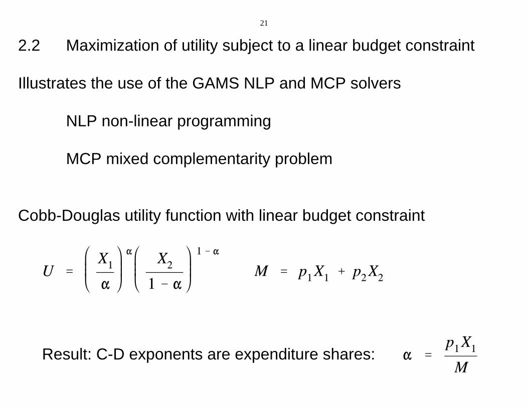
2.2 Maximization of utility subject to a linear budget constraint

Illustrates the use of the GAMS NLP and MCP solvers

NLP non-linear programming

MCP mixed complementarity problem

Cobb-Douglas utility function with linear budget constraint

Result: C-D exponents are expenditure shares:

22

“Primal” formulation as an optimization problem

z

z

z

Can solve for “Marshallian” or “uncompensated” demand functions

23

“Dual” formulation as a minimization problem

z

z

z

Can solve for “Hicksian” or “compensated” demand functions

C:\jim\COURSES\8858\code-bk 2012\M2-2.gms Monday, January 09, 2012 3:34:24 AM Page 1

$TITLE: M2-2.GMS: consumer choice, modeled as an NLP and a MCP* maximize utility subject to a linear budget constraint* two goods, Cobb-Douglas preferences

$ONTEXTThis program introduces economic students to GAMS and GAMS solvers.The problem itself is known and loved by all econ students from undergraduate intermediate micro economics on up:Maximizing utility with two goods and a linear budget constraint.

Four versions are considered OPTIMIZE: direct constrained optimization using the NLP (non-linear programming) solver COMPLEM: uses the first-order conditions (FOC) to create a square system of n inequalities in n unknowns, solved using the MCP (mixed complementarity problem) solver COMPLEM2: instead of the utility function and FOC, uses the expenditure function and Marshallian demand functions, solved as an MCP COMPLEM3: instead of the utility function and FOC, uses the expenditure function and Hicksian demand functions, solved as an MCP$OFFTEXT

PARAMETERS M Income P1, P 2 prices of goods X1 and X2 S1, S 2 utility shares of X1 and X2;


M = 100;P1 = 1;P2 = 1;S1 = 0.5;S2 = 0.5;

NONNEGATIVE VARIABLES

X1, X 2 Commodity demands L A M B D A Lagrangean multiplier (marginal utility of income);

VARIABLES

U Welfare;

EQUATIONS

U T I L I T Y Utility I N C O M E Income-expenditure constraint FOC1, F O C 2 First-order conditions for X1 and X2;

UTILITY.. U =E= 2*(X1**S1)*(X2**S2);

INCOME.. M =G= P1*X1 + P2*X2;


FOC1.. LAMBDA*P1 =G= 2*S1*X1**(S1-1)*(X2**S2);

FOC2.. LAMBDA*P2 =G= 2*S2*X2**(S2-1)*(X1**S1);

* set starting valuesU.L = 100;X1.L = 50;X2.L = 50;LAMBDA.L = 1;

* modeled as a non-linear programming problem

MODEL OPTIMIZE /UTILITY, INCOME/;SOLVE OPTIMIZE USING NLP MAXIMIZING U;

* modeled as a complementarity problem

MODEL COMPLEM /UTILITY.U, INCOME.LAMBDA, FOC1.X1, FOC2.X2/;SOLVE COMPLEM USING MCP;

* counterfactuals

P1 = 2;

SOLVE OPTIMIZE USING NLP MAXIMZING U;


SOLVE COMPLEM USING MCP;

P1 = 1;M = 200;

SOLVE OPTIMIZE USING NLP MAXIMZING U;SOLVE COMPLEM USING MCP;

* now use the expenditure function, giving the minimum cost of buying* one unit of utility: COSTU = P1**S1 * P2**S2 = PU* where PU is the "price" of utility: the inverse of lambda* two versions are presented:* one using Marshallian (uncompensated) demand: X_i = F_i(P1, P2, M)* one using Hicksian (compensated) demand: X_i = F_i(P1, P2, U)

P1 = 1;M = 100;

NONNEGATIVE VARIABLES P U price of utility;

EQUATIONS C O S T U expenditure function: cost of producing utility = PU D E M A N D M 1 Marshallian demand for good 1 D E M A N D M 2 Marshallian demand for good 2


D E M A N D H 1 Hicksian demand for good 1 D E M A N D H 2 Hicksian demand for good 2 D E M A N D U Demand for utility (indirect utility function);

COSTU.. P1**S1 * P2**S2 =G= PU;

DEMANDM1.. X1 =G= S1*M/P1;

DEMANDM2.. X2 =G= S2*M/P2;

DEMANDH1.. X1 =G= S1*PU*U/P1;


DEMANDU.. U =E= M/PU;

PU.L = 1;

MODEL C O M P L E M 2 m a r s h a l l /COSTU.U, DEMANDM1.X1, DEMANDM2.X2, DEMANDU.PU/;MODEL C O M P L E M 3 h i c k s /COSTU.U, DEMANDH1.X1, DEMANDH2.X2, DEMANDU.PU/;

SOLVE COMPLEM2 USING MCP;SOLVE COMPLEM3 USING MCP;

* counterfactuals


P1 = 2;


P1 = 1;M = 200;


23

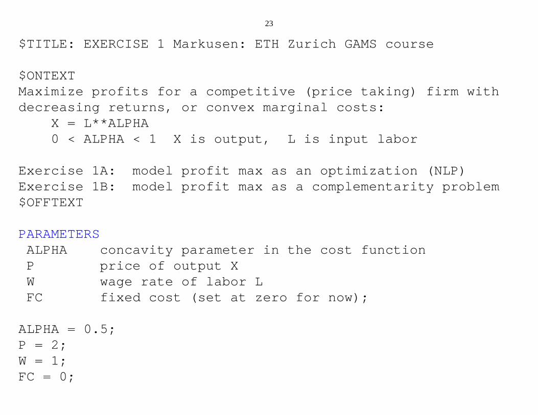
$TITLE: EXERCISE 1 Markusen: ETH Zurich GAMS course

$ONTEXTMaximize profits for a competitive (price taking) firm withdecreasing returns, or convex marginal costs: X = L**ALPHA 0 < ALPHA < 1 X is output, L is input labor

Exercise 1A: model profit max as an optimization (NLP)Exercise 1B: model profit max as a complementarity problem$OFFTEXT

PARAMETERS ALPHA concavity parameter in the cost function P price of output X W wage rate of labor L FC fixed cost (set at zero for now);

ALPHA = 0.5;P = 2;W = 1;FC = 0;

24

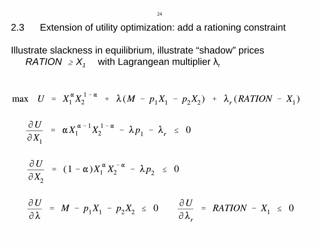
2.3 Extension of utility optimization: add a rationing constraint

Illustrate slackness in equilibrium, illustrate “shadow” pricesRATION $ X1 with Lagrangean multiplier 8r


$TITLE: M2-3.GMS add a rationing constraint to model M2-2* MAXIMIZE UTILITY SUBJECT TO A LINEAR BUDGET CONSTRAINT* PLUS RATIONING CONSTRAINT ON X1* two goods, Cobb-Douglas preferences

PARAMETERS M Income P1, P 2 prices of goods X1 and X2 S1, S 2 util shares of X1 and X2 R A T I O N rationing constraint on the quantity of X1;

M = 100;P1 = 1;P2 = 1;S1 = 0.5;S2 = 0.5;RATION = 100.;

NONNEGATIVE VARIABLES X1, X 2 Commodity demands L A M B D A I Lagrangean multiplier (marginal utility of income) L A M B D A R Lagrangean mulitplier on rationing constraint;

VARIABLES U Welfare;


EQUATIONS U T I L I T Y Utility I N C O M E Income-expenditure constraint R A T I O N 1 Rationing contraint on good X1 FOC1, F O C 2 First-order conditions for X1 and X2;

UTILITY.. U =E= 2*(X1**S1)*(X2**S2);

INCOME.. M =G= P1*X1 + P2*X2;

RATION1.. RATION =G= X1;

FOC1.. LAMBDAI*P1 + LAMBDAR =G= 2*S1*X1**(S1-1)*(X2**S2);

FOC2.. LAMBDAI*P2 =G= 2*S2*X2**(S2-1)*(X1**S1);

* modeled as a non-linear programming problem* set starting values

U.L = 100;X1.L = 50;X2.L = 50;LAMBDAI.L = 1;LAMBDAR.L = 0;

MODEL OPTIMIZE /UTILITY, INCOME, RATION1/;


SOLVE OPTIMIZE USING NLP MAXIMIZING U;

* modeled as a complementarity problem

MODEL COMPLEM /UTILITY.U, INCOME.LAMBDAI, RATION1.LAMBDAR, FOC1.X1, FOC2.X2/;SOLVE COMPLEM USING MCP;

* try binding rationing constraint at X1 <= RATION = 25;

RATION = 25;SOLVE OPTIMIZE USING NLP MAXIMIZING U;SOLVE COMPLEM USING MCP;

* show that shadow price of rationing constraint increases with income* could lead to a black market in rationing coupons, "scalping" tickets

M = 200;SOLVE OPTIMIZE USING NLP MAXIMIZING U;SOLVE COMPLEM USING MCP;

* illustrate the mpec solver* suppose we want to enforce the rationing contraint via licenses for X1* consumers are given an allocation of licenses which is RATION


* PLIC is an endogenous variables whose value is the license price* the value of the rationing license allocation should be treated as* part of income

NONNEGATIVE VARIABLES PLIC;

EQUATIONS INCOMEa FOC1a;

M = 100;RATION = 25;U.L = 100;X1.L = 25;X2.L = 75;PLIC.L = 0.1;

INCOMEa.. M + (PLIC*RATION) =E= (P1 + PLIC)*X1 + P2*X2 ;

FOC1a.. LAMBDAI*(P1 + PLIC) =G= 2*S1*X1**(S1-1)*(X2**S2);

MODEL M P E C /UTILITY, INCOMEa.LAMBDAI, FOC1a.X1, FOC2.X2, RATION1.PLIC/;MODEL COMPLEM2 /UTILITY.U, INCOMEa.LAMBDAI, FOC1a.X1, FOC2.X2,


RATION1.PLIC/;

OPTION MPEC = nlpec;

SOLVE MPEC USING MPEC MAXIMIZING U;SOLVE COMPLEM2 USING MCP;

M = 200;

SOLVE MPEC USING MPEC MAXIMIZING U;SOLVE COMPLEM2 USING MCP;

* now use the expenditure function, giving the minimum cost of buying* one unit of utility: COSTU = P1**S1 * P2**S2 = PU* where PU is the "price" of utility: the inverse of lambda* two versions are presented:* one using Marshallian (uncompensated) demand: Xi = F(P1, P2, M)* one using Hicksian (compensated) demand: Xi = F(P1, P2, U)

RATION = 100;M = 100;

NONNEGATIVE VARIABLES P U price of utility M 1 income inclusive of the value of rationing allocation;


EQUATIONS C O S T U expenditure function: cost of producing utility = PU D E M A N D M 1 Marshallian demand for good 1 D E M A N D M 2 Marshallian demand for good 2 D E M A N D H 1 Hicksian demand for good 1 D E M A N D H 2 Hicksian demand for good 2 D E M A N D U Demand for utility (indirect utility function) R A T I O N 1 b Rationing constraint (same as before) I N C O M E b Income balance equation;

COSTU.. (PLIC+P1)**S1 * P2**S2 =G= PU;

DEMANDM1.. X1 =G= S1*M1/(P1+PLIC);

DEMANDM2.. X2 =G= S2*M1/P2;

DEMANDH1.. X1 =G= S1*PU*U/(P1+PLIC);


DEMANDU.. U =E= M1/PU;

RATION1b.. RATION =G= X1;

INCOMEb.. M1 =E= M + PLIC*RATION;


PU.L = 1;

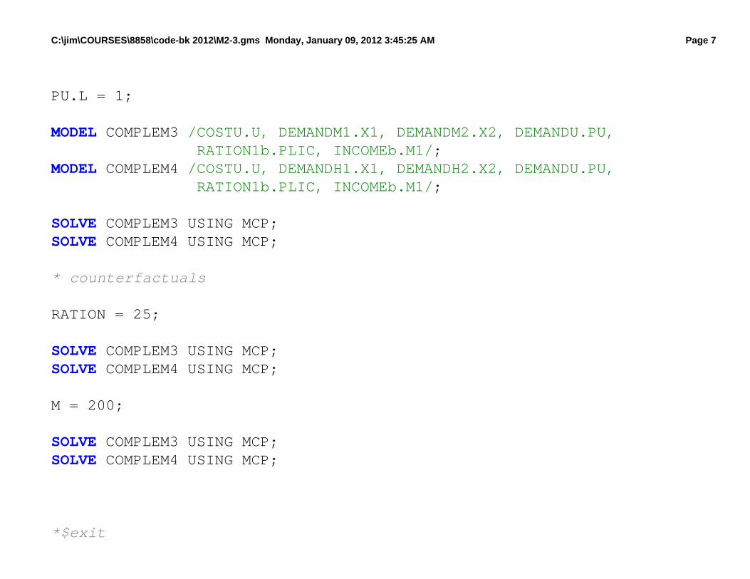
MODEL COMPLEM3 /COSTU.U, DEMANDM1.X1, DEMANDM2.X2, DEMANDU.PU, RATION1b.PLIC, INCOMEb.M1/;MODEL COMPLEM4 /COSTU.U, DEMANDH1.X1, DEMANDH2.X2, DEMANDU.PU, RATION1b.PLIC, INCOMEb.M1/;


* counterfactuals

RATION = 25;


M = 200;


*$exit


* scenario generation

SETS I indexes different values of rationing constraint /I1*I10/ J indexes income levels /J1*J10/;

PARAMETERS RLEVEL(I) PCINCOME(J) LICENSEP(I,J);

U.L = 50;X1.L = 25;X2.L = 25;PLIC.L = 0.;LAMBDAI.L = 1;

* the following is to prevent solver failure when evaluating X1**(S1-1)* at X1 = 0 (given S1-1 < 0)X1.LO = 0.01;X2.LO = 0.01;

LOOP(I,LOOP(J,

RATION = 110 - 10*ORD(I); M = 25 + 25*ORD(J);


SOLVE MPEC USING MPEC MAXIMIZING U;

RLEVEL(I) = RATION; PCINCOME(J) = M; LICENSEP(I,J) = PLIC.L;

););

DISPLAY RLEVEL, PCINCOME, LICENSEP;

$LIBINCLUDE XLDUMP LICENSEP M2-3.XLS SHEET1!B3


$TITLE: M2-4.GMS quick introduction to sets and scenarios using M2-2* MAXIMIZE UTILITY SUBJECT TO A LINEAR BUDGET CONSTRAINT* same as UTIL-OPT1.GMS but introduces set notation

SET I Prices and Goods / X1, X2 /;ALIAS (I, II);

PARAMETER M Income R A T I O N ration of X1 (constraint on max consumption of X1) P(I) prices S(I) util shares;

M = 100;P("X1") = 1;P("X2") = 1;S("X1") = 0.5;S("X2") = 0.5;RATION = 100;

NONNEGATIVE VARIABLES

X(I) Commodity demands L A M B D A I Marginal utility of income (Lagrangean multiplier) L A M B D A R Marginal effect of ration constraint;


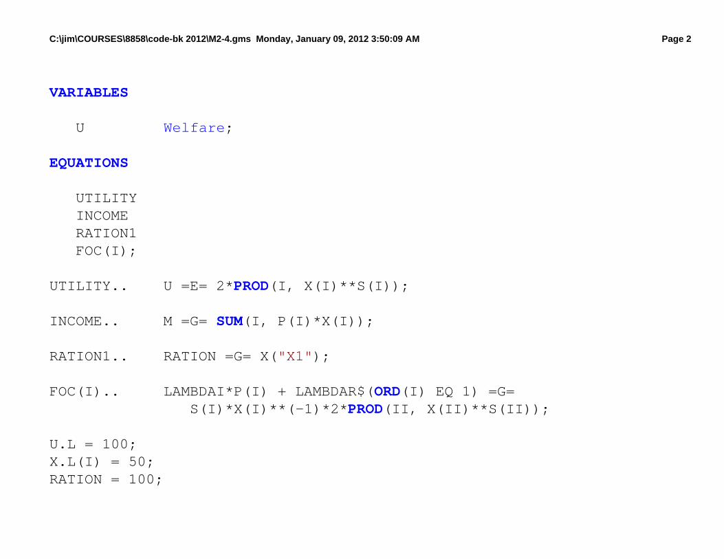
VARIABLES

U Welfare;

EQUATIONS

UTILITY INCOME RATION1 FOC(I);

UTILITY.. U =E= 2*PROD(I, X(I)**S(I));

INCOME.. M =G= SUM(I, P(I)*X(I));

RATION1.. RATION =G= X("X1");

FOC(I).. LAMBDAI*P(I) + LAMBDAR$(ORD(I) EQ 1) =G= S(I)*X(I)**(-1)*2*PROD(II, X(II)**S(II));

U.L = 100;X.L(I) = 50;RATION = 100;


* first, solve the model as an nlp, max U subject to income* rationing constraint in non-binding

MODEL UMAX /UTILITY, INCOME, RATION1/;SOLVE UMAX USING NLP MAXIMIZING U;

* second, solve the model as an mcp, using the two FOC and incomeLAMBDAI.L = 1;LAMBDAR.L = 0;

MODEL COMPLEM /UTILITY.U, INCOME.LAMBDAI, RATION1.LAMBDAR, FOC.X/;SOLVE COMPLEM USING MCP;

* scenario generationSETS J indexes different values of rationing constraint /J1*J10/;

PARAMETERS RLEVEL(J) WELFARE(J) LAMRATION(J) RESULTS(J, *);

LOOP(J, RATION = 110 - 10*ORD(J);


SOLVE COMPLEM USING MCP;

RLEVEL(J) = RATION; WELFARE(J) = U.L; LAMRATION(J) = LAMBDAR.L;

);

RESULTS(J, "RLEVEL") = RLEVEL(J);RESULTS(J, "WELFARE") = WELFARE(J);RESULTS(J, "LAMRATION") = LAMRATION(J);

DISPLAY RLEVEL, WELFARE, LAMRATION, RESULTS;

$LIBINCLUDE XLDUMP RESULTS M2-3.XLS SHEET2!B3

p

pi+1 = pi - [e'(pi)]-1e(pi) (generalizes to nxn)

p0

(1) initial guess: p0

(2) calculate e(p0) and e'(p0) (exit if |e(p0)| < ε)

(3) follow gradient path to e = 0

(4) new guess p1 implicitly given by e(p0)/(p0 - p1) = e'(p0)

e(p0)

p1

p2e(p2)

Illustration of gradient method: find the zero of the excess supply function: e(p*) = s(p*) - d(p*) = 0

e(p)

e(p1)

iteration rule:pi+1 = pi - [e'(pi)]-1e(pi)

slope = e'(p0)

p*

economic equilibrium and optimization problems using...

Documents