optimization, equilibrium and computation for energy...

Optimization, Equilibrium and Computation for EnergyEconomics

Michael C. Ferris

University of Wisconsin, Madison

Aurora Energy Research, Oxford, UKSeptember 22, 2017

Ferris (Univ. Wisconsin) Equilibrium and Energy Economics Supported by DOE/ARPA-E 1 / 31

Power generation, transmission and distribution

Determine generators’ output to reliably meet the loadI∑

Gen MW ≥∑

Load MW, at all times.I Power flows cannot exceed lines’ transfer capacity.


Single market, single good: equilibrium

Walras: 0 ≤ s(π)− d(π) ⊥ π ≥ 0

Market design and rules tofoster competitivebehavior/efficiency

Spatial extension: LocationalMarginal Prices (LMP) at nodes(buses) in the network

Supply arises often from a generatoroffer curve (lumpy)

Technologies and physics affectproduction and distribution


Satellite data, FERC and Reserves

Solar transmittance and power

9

Figure 1: This figure illustrates how the CLAVR-x retrievals will be used to provide a regime dependent bias correction to the CAPS ensemble mean cloud forecast by considering a specific time period (19:00 GMT on May 15, 2012). The upper left panel shows the CLAVR-x cloud transmittance retrieval, binned into the CAPS ensemble model 4km grid. The locations of solar (red) and wind (black) power generation facilities are indicated by the circles. The upper right panel shows the CAPS ensemble mean cloud transmittance forecast and the lower right panel shows the estimated uncertainty in the CAPS ensemble transmittance forecast (%) based on the ensemble variance. The lower left panel shows the median and standard deviations of the observed (black) and forecast (red) transmittance for each observed cloud regime (clear, probably clear, fog, water cloud, super cooled water, mixed water/ice, opaque ice, cirrus, overlap, and overshooting). Clear scenes have a transmission of 1 meaning that all the incident solar radiation reaches the surface. Opaque ice clouds are found in regions of extensive high cloudiness (Eastern Texas for example) and have the lowest transmittance, meaning that much of the solar radiation does not reach the surface. The CAPS ensemble mean transmittance is found to be systematically low for all cloud regimes with the largest biases found for fog and low cloud scenes. Relatively low biases are found for opaque ice clouds. However, the uncertainty in the CAPS ensemble mean transmittance is largest for low transmittance clouds.

Generators set asidecapacity for“contingencies” (reserves)

Separate energy πd andreserve πr prices

Use 12 hour cloud coverforecasts to reducereserves

Federal Energy RegulatoryCommission (FERC) contract tobuild models and data

Provided on NEOS (Networkenabled optimization system)

0 20 40 60 80 100 120 140 160 180

0

20

40

60

80

100

120

140

160

180

200

Columns

Row

s

Base Case

Contingency 1, time 0



Base Case

Contingency 1

Contingency 2

SCED Feasible Region

Cost-minimizing

direction

SCED optimal point

ED optimal point

Integrate satellite forecast datawith power system data and smokemodels to provide reliability andsavings outcomes


The PIES Model (Hogan) - Optimal Power Flow (OPF)

minx

c(x) cost

s.t. Ax ≥ q balance

Bx = b, x ≥ 0 technical constr

q = d(π): issue is that π is the multiplier on the “balance” constraint

Such multipliers (LMP’s) are critical to operation of market

Can try to solve the problem iteratively (shooting method):

πnew ∈ multiplier(OPF (d(π)))


The PIES Model (Hogan) - Optimal Power Flow (OPF)

minx

c(x) cost

s.t. Ax ≥ d(π) balance

Bx = b, x ≥ 0 technical constr

q = d(π): issue is that π is the multiplier on the “balance” constraint

Such multipliers (LMP’s) are critical to operation of market

Can try to solve the problem iteratively (shooting method):

πnew ∈ multiplier(OPF (d(π)))


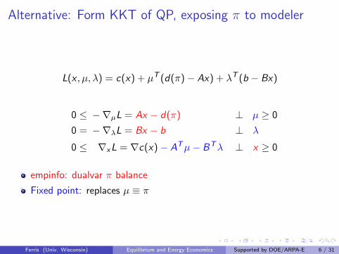
Alternative: Form KKT of QP, exposing π to modeler

L(x , µ, λ) = c(x) + µT (d(π)− Ax) + λT (b − Bx)

0 ≤ −∇µL = Ax − d(π) ⊥ µ ≥ 0

0 = −∇λL = Bx − b ⊥ λ

0 ≤ ∇xL = ∇c(x)− ATµ− BTλ ⊥ x ≥ 0

empinfo: dualvar π balance

Fixed point: replaces µ ≡ π


Alternative: Form KKT of QP, exposing π to modeler

0 ≤ Ax − d(π) ⊥ π ≥ 0

0 = Bx − b ⊥ λ

0 ≤ ∇c(x)− ATπ − BTλ ⊥ x ≥ 0

empinfo: dualvar π balance

Fixed point: replaces µ ≡ πLCP/MCP is then solvable using PATH

z =

πλx

, F (z) =

AB

−AT −BT

z +

−d(π)−b∇c(x)

Existence, uniqueness, stability from variational analysis

EMP does this automatically from the annotations


Other applications of complementarity

Complementarity can model fixed points and disjunctions

Economics: Walrasian equilibrium (supply equals demand), taxes andtariffs, computable general equilibria, option pricing (electricitymarket), airline overbooking

Transportation: Wardropian equilibrium (shortest paths), selfishrouting, dynamic traffic assignment

Applied mathematics: Free boundary problems

Engineering: Optimal control (ELQP)

Mechanics: Structure design, contact problems (with friction)

Geology: Earthquake propagation

Good solvers exist for large-scale instances of Complementarity Problems


Extension: MOPEC

minxiθi (xi , x−i , π) s.t. gi (xi , x−i , π) ≤ 0,∀i

π solves h(x , π) = 0

equilibrium

min theta(1) x(1) g(1)

...

min theta(m) x(m) g(m)

vi h pi

(Generalized) Nash

Reformulateoptimization problem asfirst order conditions(complementarity)

Use nonsmooth Newtonmethods to solve

Solve overall problemusing “individualoptimizations”?

Trade/Policy Model (MCP)

•  Split model (18,000 vars) via region

•  Gauss-Seidel, Jacobi, Asynchronous •  87 regional subprobs, 592 solves

= +


Perfect competition

maxxi

πT xi − ci (xi ) profit

s.t. Bixi = bi , xi ≥ 0 technical constr

0 ≤π ⊥∑i

xi − d(π) ≥ 0

When there are many agents, assume none can affect π by themselves

Each agent is a price taker

Two agents, d(π) = 24− π, c1 = 3, c2 = 2

KKT(1) + KKT(2) + Market Clearing gives ComplementarityProblem

x1 = 0, x2 = 22, π = 2


Cournot: two agents (duopoly)

maxxi

p(∑j

xj)T xi − ci (xi ) profit

s.t. Bixi = bi , xi ≥ 0 technical constr

Cournot: assume each can affect π by choice of xi

Inverse demand p(q): π = p(q) ⇐⇒ q = d(π)

Two agents, same data

KKT(1) + KKT(2) gives Complementarity Problem

x1 = 20/3, x2 = 23/3, π = 29/3

Exercise of market power (some price takers, some Cournot, evenStackleberg)


Computational issue: PATH

Cournot model: |A| = 5

Size n = |A| ∗ Na

Size (n) Time (secs)

1,000 35.42,500 294.85,000 1024.6

0 10 20 30 40 50 60 70 80 90 100nz = 10403

0

10

20

30

40

50

60

70

80

90

100

Jacobian nonzero patternn = 100, Na = 20


Computation: implicit functions and local variables

Use implicit fn: z(x) =∑

j xj(and local aggregation)

Generalization to F (z , x) = 0 (viaadjoints)

empinfo: implicit z F

Size (n) Time (secs)

1,000 0.52,500 0.85,000 1.6

10,000 3.925,000 17.750,000 52.3

0 20 40 60 80 100nz = 333

0

20

40

60

80

100

Jacobian nonzero patternn = 100, Na = 20


A Simple Network Model

Load segments srepresent electrical loadat various instances

d sn Demand at node n in

load segment s (MWe)

X si Generation by unit i

(MWe)

F sL Net electricity

transmission on link L(MWe)

Y sn Net supply at node n

(MWe)

πsn Wholesale price ($ perMWhe)

n1

n2

n3

n13

n14n15

n16

n4n5 n6

n7

n8

n9n10

n11n12

GCSWQLD

VIC

1989

1601

1875

2430 3418

3645

6866

4860

2478

6528

1487

25609152435

18302309

9159151887

1887

2917

1930

180

1097

1930


Nodes n, load segments s, generators i , Ψ is node-generator map

maxX ,F ,d ,Y

∑s

(W (d s(λs))−

∑i

ci (Xsi )

)s.t. Ψ(X s)− d s(λs) = Y s

0 ≤ X si ≤ X i , G i ≥

∑s

X si

Y ∈ X

where the network is described using:

X =

Y : ∃F ,F s = HY s ,−F s ≤ F s ≤ F

s,∑n

Y sn ≥ 0,∀s

Key issue: decompose. Introduce multiplier πs on supply demandconstraint (and use λs := πs)

How different approximations of X affect the overall solution


Case H: Loop flow model

maxd

∑s

(W (d s(λs))− πsd s(λs))

+ maxX

∑s

(πsΨ(X s)−

∑i

ci (Xsi )

)s.t. 0 ≤ X s

i ≤ X i , G i ≥∑s

X si

+ maxY

∑s

−πsY s

s.t.∑i

Y si ≥ 0,−F s ≤ HY s ≤ F

s

πs ⊥ Ψ(X s)− d s(λs)− Y s = 0


Let A be the node-arc incidence matrix, H be the shift matrix, L be theloop constraint matrix. Standard results show:

X = Y : ∃F ,F = HY ,F ∈ F

X =Y : ∃(F , θ),Y = AF ,BAT θ = F , θ ∈ Θ,F ∈ F

X = Y : ∃F ,Y = AF ,LF = 0,F ∈ F


Loopflow model (using A,L)

maxd

∑s


+ maxX

∑s

(πsΨ(X s)−

∑i

ci (Xsi )

)s.t. 0 ≤ X s

i ≤ X i , G i ≥∑s

X si

+ maxF ,Y

∑s

−πsY s

s.t. Y s = AF s ,LF s = 0,−F s ≤ F s ≤ Fs

πs ⊥ Ψ(X s)− d s(λs)− Y s = 0


Network modelDrop loop constraints:

maxd

∑s


+ maxX

∑s

(πsΨ(X s)−

∑i

ci (Xsi )

)s.t. 0 ≤ X s

i ≤ X i , G i ≥∑s

X si

+ maxF ,Y

∑s

−πsY s

s.t. Y s = AF s ,−F s ≤ F s ≤ Fs

πs ⊥ Ψ(X s)− d s(λs)− Y s = 0


Comparing Network and Loopflow: DemandHere we look at simulations which impose a proportional reduction intransmission across the network. The network and loopflow modelsdemonstrate similar responses:

0

1

2

3

4

5

6

0 10 20 30 40 50 60 70 80 90 (blank) 0 10 20 30 40 50 60 70 80 90 (blank)

loopflow network

n8

n6

n7

n14

n11

n3

n9

n1

n13

n2

n15

n10

n12

n5

n16

n4

n14_n15

n9_n12

n8_n12

n13_n14

n1_n2

n16_VIC

gc_n1

n13_n15

n11_n14

n2_n3


Comparing Network and Loopflow: GenerationLikewise, generation is similar in the two models:

0

1

2

3

4

5

6

7

8

9

10

0 10 20 30 40 50 60 70 80 90 (blank) 0 10 20 30 40 50 60 70 80 90 (blank)

loopflow network

GC

gc_n1

n1

n1_n2

n10

n11

n11_n12

n11_n14

n12

n12_n13

n13

n13_n14

n13_n15

n14

n14_n15

n15

n15_n16

n16

n16_VIC

n2

n2_n3

n3

n3_n4

n4

n4_n5

n4_n6


Comparing Network and Loopflow: TransmissionNetwork transmission levels reveal that the two models are quite different:

0

20

40

60

80

100

120

0 10 20 30 40 50 60 70 80 90 (blank) 0 10 20 30 40 50 60 70 80 90 (blank)

loopflow network

n3_n4

n5_n8

n7_n8

n8_n9

n9_n12

n11_n14

n12_n13

n4_n6

n2_n3

n13_n14

n4_n5

n8_n12

n13_n15

n8_n11

n9_n10

n11_n12

n6_n7

n14_n15

n1_n2

n5_n9

n15_n16

gc_n1

swqld_n2

n16_VIC


The Game: update red, blue and purple components

maxd

∑s


+ maxX

∑s

(πsΨ(X s)−

∑i

ci (Xsi )

)s.t. 0 ≤ X s

i ≤ X i , G i ≥∑s

X si

+ maxY

∑s

−πsY s

s.t.∑i

Y si ≥ 0,−F s ≤ HY s ≤ F

s

πs ⊥ Ψ(X s)− d s(λs)− Y s = 0


Top down/bottom up

λs = πs so use complementarity to expose (EMP: dualvar)

Change interaction via new price mechanisms

All network constraints encapsulated in (bottom up) NLP (or itsapproximation by dropping LF s = 0):

maxF ,Y

∑s

−πsY s

s.t. Y s = AF s ,LF s = 0,−F s ≤ F s ≤ Fs

Could instead use the NLP over Y with HClear how to instrument different behavior or different policies ininteractions (e.g. Cournot, etc) within EMP

Can add additional detail into top level economic model describingconsumers and producers

Can solve iteratively using SELKIE


PricingOur implementation of the heterogeneous demand model incorporatesthree alternative pricing rules. The first is average cost pricing, defined by

Pacp =

∑jn∈Racp

∑s pjnsqjns∑

jn∈Racp

∑s qjns

The second is time of use pricing, defined by:

Ptous =

∑jn∈Rtou

pjnsqjns∑jn∈Rtou

qjns

The third is location marginal pricing corresponding to the wholesaleprices denoted Pns above. Prices for individual demand segments are thenassigned:

pjns =

Pacp (jn) ∈ Racp

Ptous (jn) ∈ Rtou

Pns (jn) ∈ Rlmp


Smart Metering Lowers the Cost of Congestion

0

0.5

1

1.5

2

2.5

3

3.5

4

10 20 30 40 50 60 70 80 90

acp

toup

lmp


Other specializations and extensions

minxiθi (xi , x−i , z(xi , x−i ), π) s.t. gi (xi , x−i , z , π) ≤ 0, ∀i , f (x , z , π) = 0

π solves VI(h(x , ·),C )

NE: Nash equilibrium (no VI coupling constraints, gi (xi ) only)

GNE: Generalized Nash Equilibrium (feasible sets of each playersproblem depends on other players variables)

Implicit variables: z(xi , x−i ) shared

Shared constraints: f is known to all (many) players

Force all shared constraints to have same dual variable (VI solution)

Can use EMP to write all these problems, and convert to MCP form

Use models to evaluate effects of regulations and theirimplementation in a competitive environment


Economic Application

Model is a partial equilibrium, geographic exchange model.

Goods are distinguished by region of origin.

There is one unit of region r goods.

These goods may be consumed in region r or they may be exported.

Each region solves:

minX ,Tr

fr (X ,T ) s.t. H(X ,T ) = 0, Tj = Tj , j 6= r

where fr (X ,T ) is a quadratic form and H(X ,T ) defines X uniquelyas a function of T , the taxes and tariffs.

H(X ,T ) defines an equilibrium; here it is simply a set of equations,not a complementarity problem

Applications: Brexit, modified GATT, Russian Sanctions


Model statistics and performance comparison of the EPEC

MCP statistics according to the shared variable formulation

Replication Switching Substitution

12,144 rows/cols 6,578 rows/cols 129,030 rows/cols544,019 non-zeros 444,243 non-zeros 3,561,521 non-zeros

0.37% dense 1.03% dense 0.02% dense

PATH Shared variable formulation (major, time)crash spacer prox Replication Switching Substitution

X X 7 iters 20 iters 20 iters8 secs 22 secs 406 secs

X 24 iters 22 iters 21 iters376 secs 19 secs 395 secs

X 8 iters 8 iters 8 iters28 secs 18 secs 219 secs


Results

Gauss-Seidel residualsIteration deviation

1 3.149302 0.909703 0.142244 0.022855 0.003736 0.000617 0.000108 0.000029 0.00000

Tariff revenueregion SysOpt MOPEC

1 0.117 0.0122 0.517 0.4073 0.496 0.2144 0.517 0.4075 0.117 0.012

Note that competitive solution produces much less revenue thansystem optimal solution

Model has non-convex objective, but each subproblem is solvedglobally (lindoglobal)


What is EMP?

Annotates existing equations/variables/models for modeler toprovide/define additional structure

equilibrium

vi (agents can solve min/max/vi)

bilevel (reformulate as MPEC, or as SOCP)

dualvar (use multipliers from one agent as variables for another)

QS functions (both in objectives and constraints)

implicit functions and shared constraints

Currently available within GAMS

Some solution algorithms implemented in modeling system -limitations on size, decomposition and advanced algorithms

Can evaluate effects of regulations and their implementation in acompetitive environment


Conclusions

Showed equilibrium problems built from interacting optimizationproblems

Equilibrium problems can be formulated naturally and modeler canspecify who controls what

It’s available (in GAMS)

Allows use and control of dual variables / prices

MOPEC facilitates easy “behavior” description at model level

Enables modelers to convey simple structures to algorithms andallows algorithms to exploit this

New decomposition algorithms available to modeler (Gauss Seidel,Randomized Sweeps, Gauss Southwell, Grouping of subproblems)

Can evaluate effects of regulations and their implementation in acompetitive environment

Stochastic equilibria - clearing the market in each scenario

Ability to trade risk using contracts


Hydro-Thermal System (Philpott/F./Wets)

Let us assume that 1 > 0 and p(!)2(!) > 0 for every ! 2 . This corresponds toa solution of SP meeting the demand constraints exactly, and being able to save moneyby reducing demand in each time period and in each state of the world. Under this as-sumption TP(i) and HP(i) also have unique solutions. Since they are convex optimizationproblems their solution will be determined by their Karush-Kuhn-Tucker (KKT) condi-tions. We dene the competitive equilibrium to be a solution to the following variationalproblem:

CE: (u1(i); u2(i; !)) 2 argmaxHP(i), i 2 H(v1(j); v2(j; !)) 2 argmaxTP(j), j 2 T0

Pi2H Ui (u1(i)) +

Pj2T v1(j) d1 ? 1 0;

0 +P

i2H Ui (u2(i; !)) +P

j2T v2(j; !) d2(!) ? 2(!) 0; ! 2 :

This gives the following result.

Proposition 2 Suppose every agent is risk neutral and has knowledge of all deterministicdata, as well as sharing the same probability distribution for inows. Then the solutionto SP is the same as the solution to CE.

3.1 Example

Throughout this paper we will illustrate the concepts using the hydro-thermal systemwith one reservoir and one thermal plant, as shown in Figure 1. We let thermal cost be

Figure 1: Example hydro-thermal system.

C (v) = v2, and dene

U(u) = 1:5u 0:015u2

V (x) = 30 3x+ 0:025x2

We assume inow 4 in period 1, and inows of 1; 2; : : : ; 10 with equal probability in eachscenario in period 2. With an initial storage level of 10 units this gives the competitiveequilibrium shown in Table 1. The central plan that maximizes expected welfare (byminimizing expected generation and future cost) is shown in Table 2. One can observethat the two solutions are identical, as predicted by Proposition 2.

6

Competing agents (consumers, or generators in energy market)

Each agent minimizes objective independently (cost)

Market prices are function of all agents activities


Simple electricity “system optimization” problem

SO: maxdk ,ui ,vj ,xi≥0

∑k∈K

Wk(dk)−∑j∈T

Cj(vj) +∑i∈H

Vi (xi )

s.t.∑i∈H

Ui (ui ) +∑j∈T

vj ≥∑k∈K

dk ,

xi = x0i − ui + h1i , i ∈ H

ui water release of hydro reservoir i ∈ Hvj thermal generation of plant j ∈ Txi water level in reservoir i ∈ Hprod fn Ui (strictly concave) converts water release to energy

Cj(vj) denote the cost of generation by thermal plant

Vi (xi ) future value of terminating with storage x (assumed separable)

Wk(dk) utility of consumption dk


Decomposition by prices π

maxdk ,ui ,vj ,xi≥0

∑k∈K

Wk(dk)−∑j∈T

Cj(vj) +∑i∈H

Vi (xi )

+ πT

∑i∈H

Ui (ui ) +∑j∈T

vj −∑k∈K

dk

s.t. xi = x0i − ui + h1i , i ∈ H

Problem then decouples into multiple optimizations∑k∈K

maxdk≥0

(Wk (dk)− πTdk) +∑j∈T

maxvj≥0

(πT vj − Cj(vj))

+∑i∈H

maxui ,xi≥0

(πTUi (ui ) + Vi (xi ))

s.t. xi = x0i − ui + h1i


SO equivalent to CE (price takers)

Perfectly competitive (Walrasian) equilibrium is a MOPEC

CE: Consumers k ∈ K solve CP(k) : maxdk≥0

Wk (dk)− πTdk

Thermal plants j ∈ T solve TP(j) : maxvj≥0

πT vj − Cj(vj)

Hydro plants i ∈ H solve HP(i) : maxui ,xi≥0

πTUi (ui ) + Vi (xi )

s.t. xi = x0i − ui + h1i

0 ≤ π ⊥∑i∈H

Ui (ui ) +∑j∈T

vj ≥∑k∈K

dk .

But in practice there is a gap between SO and CE. How to explain?


Stochastic: Agents have recourse?

Agents face uncertainties in reservoir inflows

Two stage stochastic programming, x1 is here-and-now decision,recourse decisions x2 depend on realization of a random variable

ρ is a risk measure (e.g. expectation, CVaR)

SP: min c(x1) + ρ[qT x2]

s.t. Ax1 = b, x1 ≥ 0,

T (ω)x1 + W (ω)x2(ω) ≥ d(ω),

x2(ω) ≥ 0,∀ω ∈ Ω.

A

T W

T

igure Constraints matrix structure of 15)

problem by suitable subgradient methods in an outer loop. In the inner loop, the second-stage problem is solved for various r i g h t h a n d sides. Convexity of the master is inherited from the convexity of the value function in linear programming. In dual decomposition, (Mulvey and Ruszczyhski 1995, Rockafellar and Wets 1991), a convex non-smooth function of Lagrange multipliers is minimized in an outer loop. Here, convexity is granted by fairly general reasons that would also apply with integer variables in 15). In the inner loop, subproblems differing only in their r i g h t h a n d sides are to be solved. Linear (or convex) programming duality is the driving force behind this procedure that is mainly applied in the multi-stage setting.

When following the idea of primal decomposition in the presence of integer variables one faces discontinuity of the master in the outer loop. This is caused by the fact that the value function of an MILP is merely lower semicontinuous in general Computations have to overcome the difficulty of lower semicontinuous minimization for which no efficient methods exist up to now. In Car0e and Tind (1998) this is analyzed in more detail. In the inner loop, MILPs arise which differ in their r i g h t h a n d sides only. Application of Gröbner bases methods from computational algebra has led to first computational techniques that exploit this similarity in case of pure-integer second-stage problems, see Schultz, Stougie, and Van der Vlerk (1998).

With integer variables, dual decomposition runs into trouble due to duality gaps that typically arise in integer optimization. In L0kketangen and Woodruff (1996) and Takriti, Birge, and Long (1994, 1996), Lagrange multipliers are iterated along the lines of the progressive hedging algorithm in Rockafellar and Wets (1991) whose convergence proof needs continuous variables in the original problem. Despite this lack of theoretical underpinning the computational results in L0kketangen and Woodruff (1996) and Takriti, Birge, and Long (1994 1996), indicate that for practical problems acceptable solutions can be found this way. A branch-and-bound method for stochastic integer programs that utilizes stochastic bounding procedures was derived in Ruszczyriski, Ermoliev, and Norkin (1994). In Car0e and Schultz (1997) a dual decomposition method was developed that combines Lagrangian relaxation of non-anticipativity constraints with branch-and-bound. We will apply this method to the model from Section and describe the main features in the remainder of the present section.

The idea of scenario decomposition is well known from stochastic programming with continuous variables where it is mainly used in the mul t i s tage case. For stochastic integer programs scenario decomposition is advantageous already in the two-stage case. The idea is


Risk Measures

Modern approach tomodeling riskaversion uses conceptof risk measures

CVaRα: mean ofupper tail beyondα-quantile (e.g.α = 0.95)

VaR, CVaR, CVaR+ and CVaR-

Loss

Fre

qu

en

cy

1111 −−−−αααα

VaR

CVaR

Probability

Maximumloss

mean-risk, mean deviations from quantiles, VaR, CVaR

Much more in mathematical economics and finance literature

Optimization approaches still valid, different objectives, varyingconvex/non-convex difficulty


Two stage stochastic MOPEC (1,1,1)

CP: mind1

,d2ω

≥0p1d1 −W (d1)

+ ρC[p2ωd

2ω −W (d2

ω)]

TP: minv1

,v2ω

≥0C (v1)− p1v1

+ ρT[C (v2ω)− p2ωv

2(ω)]

HP: minu1,x1≥0

u2ω ,x2ω≥0

− p1U(u1)

+ ρH[−p2(ω)U(u2ω)− V (x2ω)

]

s.t. x1 = x0 − u1 + h1,

x2ω = x1 − u2ω + h2ω

0 ≤ p1 ⊥ U(u1) + v1 ≥ d1

0 ≤ p2ω ⊥ U(u2ω) + v2ω ≥ d2ω,∀ω


Two stage stochastic MOPEC (1,1,1)

CP: mind1,d2

ω≥0p1d1 −W (d1) + ρC

[p2ωd

2ω −W (d2

ω)]

TP: minv1,v2

ω≥0C (v1)− p1v1 + ρT

[C (v2ω)− p2ωv

2(ω)]

HP: minu1,x1≥0u2ω ,x

2ω≥0

− p1U(u1) + ρH[−p2(ω)U(u2ω)− V (x2ω)

]s.t. x1 = x0 − u1 + h1,

x2ω = x1 − u2ω + h2ω

0 ≤ p1 ⊥ U(u1) + v1 ≥ d1

0 ≤ p2ω ⊥ U(u2ω) + v2ω ≥ d2ω,∀ω


0

1

2

3

44

5

6

7

8

9

10

Single hydro, thermal andrepresentative consumer

Initial storage 10, inflow of 4 to 0,equal prob random inflows of i tonode i

Risk neutral: SO equivalent to CE(key point is that each risk set is asingleton, and that is the same asthe system risk set)

Each agent has its own riskmeasure, e.g. 0.8EV + 0.2CVaR

Is there a system risk measure?

Is there a system optimizationproblem?

min∑i

C (x1i ) + ρi(C (x2i (ω))

)????


Equilibrium or optimization?

Theorem

If (d , v , u, x) solves (risk averse) SO, then there exists a probabilitydistribution σk and prices p so that (d , v , u, x , p) solves (risk neutral)CE(σ)

(Observe that each agent must maximize their own expected profit usingprobabilities σk that are derived from identifying the worst outcomes asmeasured by SO. These will correspond to the worst outcomes for eachagent only under very special circumstances)

High initial storage level (15 units)I Worst case scenario is 1: lowest system cost, smallest profit for hydroI SO equivalent to CE

Low initial storage level (10 units)I Different worst case scenariosI SO different to CE (for large range of demand elasticities)

Attempt to construct agreement on what would be the worst-caseoutcome by trading risk


Contracts in MOPEC (Philpott/F./Wets)

Can we modify (complete) system to have a social optimum bytrading risk?

How do we design these instruments? How many are needed? Whatis cost of deficiency?

Facilitated by allowing contracts bought now, for goods deliveredlater (e.g. Arrow-Debreu Securities)

Conceptually allows to transfer goods from one period to another(provides wealth retention or pricing of ancilliary services in energymarket)

Can investigate new instruments to mitigate risk, or move to systemoptimal solutions from equilibrium (or market) solutions


Trading risk: pay σω now, deliver 1 later in ω

CP: mind1,d2

ω≥0

,tCσtC +

p1d1 −W (d1) + ρC

[p2ωd

2ω −W (d2

ω)

− tCω

]TP: min

v1,v2ω≥0

,tTσtT +

C (v1)− p1v1 + ρT

[C (v2ω)− p2ωv

2(ω)

− tTω

]HP: min

u1,x1≥0u2ω ,x

2ω≥0

,tH

σtH

− p1U(u1) + ρH

[−p2(ω)U(u2ω)− V (x2ω)

− tHω

]s.t. x1 = x0 − u1 + h1,

x2ω = x1 − u2ω + h2ω

0 ≤ p1 ⊥ U(u1) + v1 ≥ d1

0 ≤ p2ω ⊥ U(u2ω) + v2ω ≥ d2ω,∀ω

0 ≤ σω ⊥ tCω + tTω + tHω ≥ 0,∀ω σ = (σω)


Trading risk: pay σω now, deliver 1 later in ω

CP: mind1,d2

ω≥0,tCσtC + p1d1 −W (d1) + ρC

[p2ωd

2ω −W (d2

ω)− tCω

]TP: min

v1,v2ω≥0,tT

σtT + C (v1)− p1v1 + ρT

[C (v2ω)− p2ωv

2(ω)− tTω

]HP: min

u1,x1≥0u2ω ,x

2ω≥0,tH

σtH − p1U(u1) + ρH

[−p2(ω)U(u2ω)− V (x2ω)− tHω

]s.t. x1 = x0 − u1 + h1,

x2ω = x1 − u2ω + h2ω

0 ≤ p1 ⊥ U(u1) + v1 ≥ d1

0 ≤ p2ω ⊥ U(u2ω) + v2ω ≥ d2ω,∀ω

0 ≤ σω ⊥ tCω + tTω + tHω ≥ 0,∀ω σ = (σω)


Theory and Observations

agent problems are multistage stochastic optimization models

perfectly competitive partial equilibrium still corresponds to a socialoptimum when all agents are risk neutral and share commonknowledge of the probability distribution governing future inflows

situation complicated when agents are risk averseI utilize stochastic process over scenario treeI under mild conditions a social optimum corresponds to a competitive

market equilibrium if agents have time-consistent dynamic coherentrisk measures and there are enough traded market instruments (overtree) to hedge inflow uncertainty

Otherwise, must solve the stochastic equilibrium problem

Research challenge: develop reliable algorithms for large scaledecomposition approaches to MOPEC


MCP size of equilibrium problems containing sharedvariables by formulation strategy

Strategy Size of the MCP

replication (n + 2mN)switching (n + mN + m)

substitution (explicit) (n + m)substitution (implicit) (n + nm + m)

Fi (z) =

∇xi fi (x , y)− (∇xiH(y , x))µi∇yi fi (x , y)− (∇yiH(y , x))µi

H(yi , x)

, zi =

xiyiµi

.


Spacer steps

Given (x , y , µ) during iterations

Compute a unique feasible pair (y , µ)

Evaluate the residual at (x , y , µ)

Choose the point if it has less residual than the one of (x , y , µ)


Reserves, interruptible load, demand response

Generators set aside capacity for “contingencies” (reserves)

Separate energy πd and reserve πr prices

Consumers may also be able to reduce consumption for short periods

Alternative to sharp price increases during peak periods

Constraints linking energy “bids” and reserve “bids”

vj + uj ≤ Uj , uj ≤ Bjvj

Multiple scenarios - linking constraints on bids require “bid curve tobe monotone”


Price taking: model is MOPEC

Consumption dk , demand response rk , energy vj , reserves uj , prices π

Consumer max(dk ,rk )∈C

utility(dk)− πdTdk + profit(rk , πr )

Generator max(vj ,uj )∈G

profit(vj , πd) + profit(uj , πr )

s.t. vj + uj ≤ Uj , uj ≤ BjvjTransmission max

f ∈Fcongestion rates(f , πd)

Market clearing

0 ≤ πd ⊥∑j

vj −∑k

dk −Af ≥ 0

0 ≤ πr ⊥∑j

uj +∑k

rk −R ≥ 0


Large consumer is price making: MPEC

Leader/follower

Consumer max utility(dk)− πdTdk + profit(rk , πr )

with the constraints:

(dk , rk) ∈ CGenerator max

(vj ,uj )∈G′profit(vj , πd) + profit(uj , πr )

Transmission maxf ∈F

congestion rates(f , πd)

0 ≤ πd ⊥∑j

vj −∑k

dk −Af ≥ 0

0 ≤ πr ⊥∑j

uj +∑k

rk −R ≥ 0


Solution and observations

Formulate as MIP, add mononticity constraints and scenarios

New Zealand (NZEM) data, large consumer at bottom of South Island

Expected difference percentage between “wait and see” solutionsversus model solution (evaluated post optimality with simulation)

Sample Size 1 2 4 6 8

Expected diff 31.34 17.83 9.22 7.35 9.26Standard dev 22.86 9.62 4.86 7.69 6.59Bound gap (%) 0 0 0 12.7 24.8

More samples better(!)

More research to model/solve more detailed problems


Dual Representation of Risk Measures

Dual representation (of coherent r.m.) in terms of risk sets

ρ(Z ) = supµ∈D

Eµ[Z ]

If D = p then ρ(Z ) = E[Z ]

If Dα,p = λ : 0 ≤ λi ≤ pi/(1− α),∑

i λi = 1, then

ρ(Z ) = CVaRα(Z )

Special case of a Quadratic Support Function

ρ(y) = supu∈U〈u,By + b〉 − 1

2〈u,Mu〉

EMP allows any Quadratic Support Function to be defined andfacilitates a model transformation to a tractable form for solution


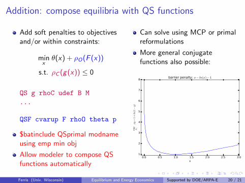
Addition: compose equilibria with QS functions

Add soft penalties to objectivesand/or within constraints:

minxθ(x) + ρO(F (x))

s.t. ρC (g(x)) ≤ 0

QS g rhoC udef B M

...

QSF cvarup F rhoO theta p

$batinclude QSprimal modnameusing emp min obj

Allow modeler to compose QSfunctions automatically

Can solve using MCP or primalreformulations

More general conjugatefunctions also possible:

0.0 0.5 1.0 1.5 2.0 2.5 3.0x

1

2

3

4

5

6

7

8

sup

R+

xy+

1+ln

(1−y)

barrier penalty: x− ln(x)− 1


The link to MOPEC

minx∈X

θ(x) + ρ(F (x))

ρ(y) = supu∈U〈u, y〉 − 1

2〈u,Mu〉

0 ∈ ∂θ(x) +∇F (x)T∂ρ(F (x)) + NX (x)

0 ∈ ∂θ(x) +∇F (x)Tu + NX (x)

0 ∈−u + ∂ρ(F (x)) ⇐⇒ 0 ∈ −F (x) + Mu + NU(u)

This is a MOPEC, and we have multiple copies of this for each agent


optimization, equilibrium and computation for energy...

Documents