Econometric Perspectives on Economic Measurement

Adam Gorajek

Research Discussion Paper

R D P 2018- 08

Figures in this publication were generated using Mathematica.

The contents of this publication shall not be reproduced, sold or distributed without the prior consent of the Reserve Bank of Australia and, where applicable, the prior consent of the external source concerned. Requests for consent should be sent to the Secretary of the Bank at the email address shown above.

ISSN 1448-5109 (Online)

The Discussion Paper series is intended to make the results of the current economic research within the Reserve Bank available to other economists. Its aim is to present preliminary results of research so as to encourage discussion and comment. Views expressed in this paper are those of the authors and not necessarily those of the Reserve Bank. Use of any results from this paper should clearly attribute the work to the authors and not to the Reserve Bank of Australia.

Enquiries:

Phone: +61 2 9551 9830 Facsimile: +61 2 9551 8033 Email: rbainfo@rba.gov.au Website: http://www.rba.gov.au

Econometric Perspectives on Economic Measurement

Adam Gorajek

Research Discussion Paper 2018-08

July 2018

Economic Research Department Reserve Bank of Australia

For their input I thank Bert Balk, Anthony Brassil, Jan de Haan, Michele De Nadai, Denzil Fiebig,

Kevin Fox, SeoJeong (Jay) Lee, Alicia Rambaldi, John Simon, Franklin Soriano, and participants at

several seminars and conferences. Rosie Wisbey sourced some elusive materials. This work forms

part of my PhD at the University of New South Wales and was supported by an Australian

Government Research Training Scholarship. The views expressed in this paper are those of the

author and do not reflect those of the Reserve Bank of Australia. Any errors are my own.

Author: gorajeka at domain rba.gov.au

Media Office: rbainfo@rba.gov.au

Abstract

It turns out that price index functions share a basic interpretation; practically all of them measure a

change in some average of quality-adjusted prices. The different options are distinguished by their

choice of average, their definition of quality, and their stance on what I label ‘equal interest’. This

new perspective updates the so-called stochastic approach to choosing index functions. It also offers

new avenues to understand and tackle measurement problems. I discuss three examples.

JEL Classification Numbers: C18, C43, C51, C80

Keywords: macroeconomic data, index number, stochastic approach, hedonic price index

Table of Contents

1. Introduction 1

2. The Standard Model Needs Changing 2

2.1 The Standard Model 2

2.2 The Literature Favours Weighted Estimators 4

2.3 The Weighted Estimators are Inconsistent 6

2.4 We Have Just Been Using the Wrong Model 8

2.5 The Literature Contains Other Related Contributions 9

3. Index Numbers Share Econometric Foundations 10

3.1 The Diewert Model Generalises Further 10

3.2 Three Choices Distinguish Price Index Functions 12

3.3 This Changes the Stochastic Approach 16

4. The New Framework Challenges Some Practices 17

4.1 The Goldberger (1968) Bias Correction is Unnecessary 17

4.2 Some Dynamic Population Methods Look Questionable 19

4.3 Unit Values Can Distort Index Number Interpretation 21

4.4 There Are Obvious Avenues for Further Progress 24

5. Conclusion 24

Appendix A: The Inconsistency Arising from Endogenous Weighting is a Linear Projection 26

Appendix B: Loosening Strict Error Exogeneity Introduces Another Avenue for Weights to Generate Inconsistency 27

Appendix C: The Model of Voltaire and Stack (1980) Equates to The Diewert Model, under Restrictive Conditions Only 28

Appendix D: Some Choices of f (x), {Utv}, and {qualitytv} are Always Equivalent 31

Appendix E: The Dutot Index Has an Unexpected Interpretation 33

Appendix F: The Method of Moments Makes Sensible Multilateral Index Functions 34

References 37

1. Introduction

All measures of macroeconomic change rely on microeconomic data. Key examples are consumer

price inflation, housing price inflation, output growth, productivity growth, and purchasing power

parities. Each come from micro data on market transactions, and each are cornerstones of evidence-

based policy.

Yet it remains unclear how the measures should handle changes in the quality composition of the

items being transacted. For instance, how should a consumer price index adjust for the improving

quality of mobile phones? What even defines quality? Measurement scholars find these questions

difficult. With technological advances delivering large quality improvements, sensible solutions are

important. Jaimovich, Rebelo and Wong (2015) show that quality compositions can swing with

business cycles as well.

When it is not the types of items being transacted that are changing – just their market shares –

the primary tools for handling quality change are index functions. The literature contains hundreds

of options and three main approaches for distinguishing among them:

1. The ‘test’ approach (also called ‘axiomatic’ or ‘instrumental’) distinguishes functions by their

ability to satisfy certain desirable mathematical properties. (Balk (2008) provides a review.)

2. The ‘economic’ approach distinguishes functions by how closely they measure the changing cost

of attaining a given economic objective, such as an amount of output or living standard.

(Diewert (1981) provides a review.)

3. The ‘stochastic’ approach distinguishes functions by how well they estimate parameters in

econometric descriptions of the measurement task. (See Selvanathan and Rao (1994) and

Clements, Izan and Selvanathan (2006) for reviews.) Currently the literature identifies only some

functions as having stochastic justifications.

When the types of items being transacted are changing, standard index functions become undefined

and alternative tools are needed. Here, extensions of the econometric methods behind the stochastic

approach have been influential.

Still, this paper shows that the relevance of econometrics to economic measurement runs a lot

deeper. It turns out that practically all price index functions have origins that are nested in the same

econometric model. Through the model we can view the functions as comparing averages of quality-

adjusted prices at different places or times. The options are distinguished by their type of average,

their definition of quality, and their stance on what I label ‘equal interest’. Following normal practice,

each price index implies a quantity index. What look like being exceptions to the paradigm are minor.

This result changes the stochastic approach in useful ways. First, by covering practically all bilateral

and multilateral price index functions, it is more comprehensive. So the approach becomes a more

complete tool for choosing among the different function types. Second, to distinguish between the

types, the approach now relies on attributes that are conceptual. Previous versions of the stochastic

approach have distinguished functions using modelling assumptions. The overall outcome is not a

2

recommendation to use any specific index functions, but a logically consistent framework for

differentiating and choosing among them.

In turn, the changes to the stochastic approach offer new avenues to understand and tackle

measurement problems. The paper highlights three examples, by challenging: the use of a bias

correction from Goldberger (1968); the widespread reliance on so-called unit values; and some

common views on adjusting for quality change when the types of transacted items are changing.

Sensible alternatives are sometimes immediate. With time, the deeper connections to the

econometrics literature could yield others.

The new framework and the results that flow from it are the paper’s main contributions. Before

establishing those results though, it is necessary to do some groundwork. In particular, the next

section demonstrates that econometric estimators in measurement applications are often

inconsistent for the parameters of interest that are defined (or ‘identified’) by the corresponding

model assumptions. Strangely, it is not the estimators that need to change, but the standard model

set-up that defines the parameters of interest. These ideas overlap with other ideas that are already

in the literature. By connecting and re-specifying them, it is hoped that a shift in the consensus on

appropriate model specification will occur.

For the wider macro community, a side-goal of the paper is to simplify issues of measurement. Macro

researchers could use the new framework to appreciate the many compromises built into macro

data. The next section is therefore also intended to provide sufficient background for macro

researchers without a specialist understanding of measurement.

2. The Standard Model Needs Changing

2.1 The Standard Model

The econometric model most commonly used to define the price measurement task descends from

pioneering work by Court (1939). Using assumptions A1 to A4, it describes pricing behaviour in some

market for differentiated product varieties. To distinguish it from a later model that will have many

of the same characteristics, call it The Standard Model.

A1

ln 1, ,tv t v tvp t T β spec (1)

where: ptv is the transaction price of variety v in time period or territory (place) t; t is a fixed

effect for t; is a vector of parameters; and specv is a vector of observed variety specifications.

Hence ’specv can be seen as a control for the effect of quality on prices. tv is an error term.

A2 Across varieties the observations are independently and identically distributed.

A3 The errors are strictly exogenous. So

0tv v t spec (2)

3

A4 Other technical conditions of regularity are satisfied, ruling out perfect multicollinearity and

variables with infinite second moments.

For measurement, the interest is in the differences between the t. For instance, if t is for time, 1te

indexes a time series of the price level, holding quality constant. The series is useful for

measuring inflation and deflating nominal aggregates into real ones. If t is for territory, 1te

indexes a cross-section of purchasing power parities.

Special cases of The Standard Model shape many macro indicators. Hence, a lot of empirical macro

research is linked to it somehow. Aside from variation in the concept behind t, the special cases

differ along several dimensions:

The market types vary. For instance, in official capacities The Standard Model has been applied

to the rental market in the United States (Bureau of Labor Statistics 2017), the used car market

in Germany (German Federal Statistical Office 2003), and the computer market in Australia

(Australian Bureau of Statistics 2005). It can be applied to markets that are more broadly defined

as well.

The types of regressors in specv differ. In measurement handbooks the regressors are often

variety attributes (International Labour Office et al 2004; International Labour Organization et al

2004; Eurostat 2013). In this case the model becomes ‘hedonic’. In some other cases the

regressors are variety dummies and ’specv becomes a variety fixed effect (World Bank 2013).

The population of transacted varieties can be static, with no entry or exit, or it can be dynamic.

The static case is special because t is definitionally uncorrelated with the regressors in specv.

Including ’specv is thus irrelevant for defining the population price index. This is the classic set-

up in the prevailing stochastic approach to choosing index functions, described more fully in

Section 3.3.

In measurement contexts more broadly, static populations are sometimes synthetic, in the sense

that missing varieties are assumed to have hypothetical prices. Often the hypothetical prices

correspond to predictions of T = 1 versions of The Standard Model (and where interest is not in

the t). This method is behind official price indices for mobile phones in the United Kingdom

(Office for National Statistics 2014). Since modelling considerations then change, this paper is

not about T = 1 cases, except where stated otherwise.

Still, the size of T can vary. Territory applications are often multilateral, so T ≥ 3, as in versions

that support official calculations of purchasing power parities (World Bank 2013). Time

applications are often bilateral, so T = 2. Successive 2 1e are then combined to form a longer

time series. Such is the approach behind official calculations of Australian computer price indices

(Australian Bureau of Statistics 2005).

The notation and format differs across applications in the literature. When T = 2 and the

population is static, the format is sometimes in first differences. In levels, The Standard Model

often includes a constant and the fixed effects are normalised to a base.

4

Note that in all applications the (t, v) pairs are restricted to have a single price. For housing markets,

where each home is a unique variety, the single price feature is natural if the time periods are short

enough to rule out successive sales. For most other markets it is unnatural and national statistical

offices use unit values to resolve the multiple prices problem. Section 4.3 will discuss the use of unit

values. For now the reader can ignore them.

It is often unclear whether other applications of The Standard Model really do assume strict error

exogeneity. Theoretical work on the equilibria of differentiated product markets, such as

Rosen (1974), Berry, Levinsohn and Pakes (1995), and Pakes (2003), suggests that for the general

case the assumption is too strong. Unless specv is empty and the Model consists only of t, the true

conditional expectation for price need not take the proposed linear form (see Hansen (2018, ch 2)).

For the hedonic case of The Standard Model, the same point is emphasised in Triplett (2004) and

Brachinger, Beer and Schöni (2018).

The strength of the strict exogeneity assumption is also unnecessary. For instance, according to

Diewert (2005, p 775), ‘the price statistician takes a descriptive statistics perspective’. To effect a

descriptive statistics perspective in this modelling set-up requires only that the population errors are

uncorrelated with the implied regressors. In the more formal econometric language of, for instance,

Solon, Haider and Wooldridge (2015, p 303), a ‘projection’ is sufficient.

I make the strict exogeneity assumption because weaker versions of it will only turn out to

strengthen my conclusions. It simplifies explanations as well. Later I will relax it.

2.2 The Literature Favours Weighted Estimators

After collecting, say, a large random sample of varieties, practitioners must decide how to estimate

the t.

Without more information, standard econometric practice would be to use ordinary least squares

(OLS). Indeed, OLS was used for the equivalent of a static population, T = 2 set-up as early as

Jevons (1869). In that case OLS produces what is now called a Jevons price index, i.e.

2 1

1

ˆ ˆ 21,2

1

ˆOLS OLS V

Jevonsv

v v

pe P

p

(3)

where V is the total number of unique varieties in the sample. Each price ratio (or ‘price relative’) is

given equal weight in calculating the overall price change between periods 1 and 2.

But when quantities data are also available, influential scholars have argued against using equally

weighted measures of price change for most measurement applications.

Everyone knows that pork is more important than coffee and wheat than quinine. Thus the quest for

fairness lead to the introduction of weighting. (Fisher 1922, p 43)

5

Thus if price relatives are different, then an appropriate definition of average price change cannot be

determined independently of the economic importance of the corresponding goods. (Diewert (2010,

p 252) paraphrasing Keynes (1930))

... we should use a weighted regression approach, since we are interested in an estimate of a weighted

average of the pure-price change, rather than just an unweighted average over all possible models, no

matter how peculiar or rare. (Griliches 1971, p 8)

These views have been influential. Heravi and Silver (2007, p 251) even take weighting as

‘axiomatic’. To implement weighting, the dominant preference now is to estimate the t with

weighted least squares (WLS), using weights for economic importance. Works that support or use

weighted estimation for special cases of The Standard Model include measurement handbooks from

International Labour Office et al (2004) and International Labour Organization et al (2004), an

econometric textbook by Berndt (1991), various statistical agency series, and countless research

publications, including from recent years.

The preferred weights typically relate to expenditure shares. In a static T = 2 set-up they might look

like

1 1 2 21 2

1 1 2 2

1 1

2 2

Tornqvist v v v vtv v v

v v v vv v

p q p qw s s

p q p q

(4)

where qtv is for transaction quantities and the stv are expenditure shares. Estimation then produces

an index number advocated by Törnqvist (1936), i.e.

2 1ˆ ˆ 21,2

1

ˆ

Tornqvistv

WLS WLS

w

Tornqvistv

v v

pe P

p

(5)

(Derivations of Equations (3) and (5) are in Diewert (2005).)

The Törnqvist index is common in research applications and at national statistical offices. It is, for

example, being used for an official chained measure of US consumer prices (Bureau of Labor

Statistics 2018). Assessments using the so-called economic approach to index numbers shows it to

have excellent properties (Diewert 1976). Judging by Clements et al (2006), the properties have

further promoted WLS in other applications of The Standard Model.

The handbooks from International Labour Office et al (2004, p 301) and International Labour

Organization et al (2004, p 420) also discuss an option of weighting implicitly, whereby the

probability of sampling each variety reflects its economic importance. The option is equivalent to

explicit weighting.

Either way, weighting for economic importance departs from mainstream econometric practices. For

example, it is absent from a list of econometric justifications for weighting in Solon et al (2015),

which is somewhat of a weighting handbook. Diewert (2005) also emphasises this ongoing tension

between standard measurement and econometric considerations.

6

Occasionally the stated econometric justification for the weights is that error variance is lower for

varieties with higher economic importance. For instance, Clements and Izan (1981) argue that

national statistical offices might invest more resources in making accurate price measurements of

varieties that command more spending. A pursuit of econometric efficiency could then justify

weighting. Clements and Izan (1987) later use data on Australian consumer prices to reject the error

variance hypothesis in that case.

Triplett (2004) offers another perspective, drawing on a well-known property of WLS. With

exogenous weights and assumptions A1 to A4 satisfied, WLS is consistent and unbiased, just like

OLS. Even if WLS is less efficient, in large samples the difference is negligible.

2.3 The Weighted Estimators are Inconsistent

Typically omitted from the conversation is that the weights are in fact endogenous. Expenditure

shares contain prices, which are functions of the errors. They also contain quantities, which can be

functions of the errors via prices. Either way, WLS is inconsistent because it over-represents

observations with errors of a particular sign.

The justification from Triplett (2004) breaks down because it works only for exogenous weights.

Arguments based on efficiency improvements are problematic too; even when the premise about

error variance is correct, the efficiency benefit from weighting would have to outweigh the cost of

inconsistency.

The degree of inconsistency comes from the coefficients in a so-called weighted linear projection of

the errors on the regressors. That is, using and xtv as vector shorthand for all the coefficients and

regressors that are implied in The Standard Model,

1ˆplim 0WLS

V tv tv tv tv tv tvw w

δ δ x x x (6)

Appendix A contains a derivation. The final expectation term is not zero because the wtv are functions

of the tv.

What then transmits into the price index is the difference in the inconsistencies of the estimated

fixed effects. It can be subtle. Some stylised scenarios help to develop the intuition and to set up

the eventual solution. The scenarios use small samples, so the metric for central tendency switches

momentarily to the degree of bias. The intuition is transferable.

Scenarios. From a population that is static over two periods, consider a random sample of five

varieties, like the solid dots in the left panel of Figure 1. Let the specv vector be empty, so the

spread of within-period prices comes only from the errors. In this case the strict exogeneity

assumption is trivially sensible. The ˆOLSt trace out a prediction that intersects the simple

arithmetic average of observed log prices in each period. The estimates are unbiased.

The left panel also introduces WLS, which is equivalent to cloning observations in numbers

proportional to their weight, before applying OLS. If in repeated samples the weights are

positively related to the errors as depicted, WLS will tend to trace out higher predictions for log

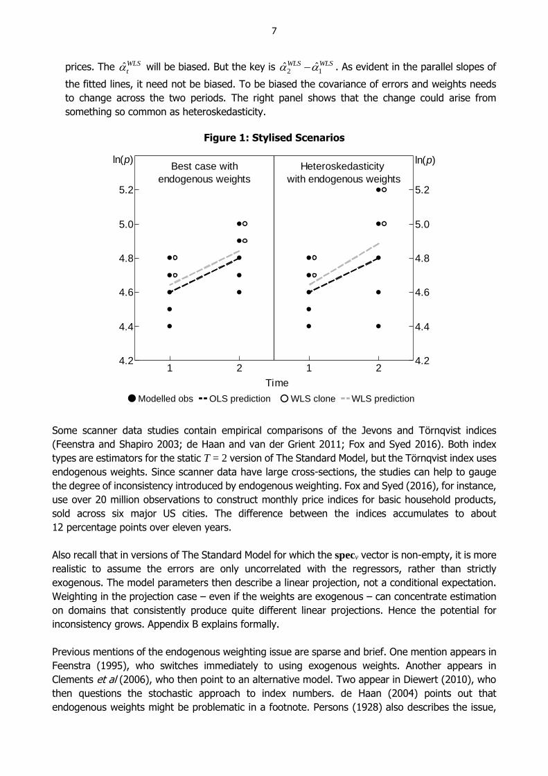
7

prices. The ˆWLSt will be biased. But the key is 2 1

ˆ ˆWLS WLS . As evident in the parallel slopes of

the fitted lines, it need not be biased. To be biased the covariance of errors and weights needs

to change across the two periods. The right panel shows that the change could arise from

something so common as heteroskedasticity.

Figure 1: Stylised Scenarios

Some scanner data studies contain empirical comparisons of the Jevons and Törnqvist indices

(Feenstra and Shapiro 2003; de Haan and van der Grient 2011; Fox and Syed 2016). Both index

types are estimators for the static T = 2 version of The Standard Model, but the Törnqvist index uses

endogenous weights. Since scanner data have large cross-sections, the studies can help to gauge

the degree of inconsistency introduced by endogenous weighting. Fox and Syed (2016), for instance,

use over 20 million observations to construct monthly price indices for basic household products,

sold across six major US cities. The difference between the indices accumulates to about

12 percentage points over eleven years.

Also recall that in versions of The Standard Model for which the specv vector is non-empty, it is more

realistic to assume the errors are only uncorrelated with the regressors, rather than strictly

exogenous. The model parameters then describe a linear projection, not a conditional expectation.

Weighting in the projection case – even if the weights are exogenous – can concentrate estimation

on domains that consistently produce quite different linear projections. Hence the potential for

inconsistency grows. Appendix B explains formally.

Previous mentions of the endogenous weighting issue are sparse and brief. One mention appears in

Feenstra (1995), who switches immediately to using exogenous weights. Another appears in

Clements et al (2006), who then point to an alternative model. Two appear in Diewert (2010), who

then questions the stochastic approach to index numbers. de Haan (2004) points out that

endogenous weights might be problematic in a footnote. Persons (1928) also describes the issue,

Best case with

endogenous weights

1 24.2

4.4

4.6

4.8

5.0

5.2

ln(p)

Ti

Modelled obs OLS prediction

Heteroskedasticity

with endogenous weights

1 24.2

4.4

4.6

4.8

5.0

5.2

ln(p)

me

WLS clone WLS prediction

8

although not using a stochastic framework. There being no systematic objection in the literature,

endogenous WLS has remained the norm.

2.4 We Have Just Been Using the Wrong Model

The temptation here is to argue again for OLS, or maybe to seek out an instrument for expenditure

shares. But the weighted estimators carefully incorporate the viewpoint of Keynes and Fisher. The

problem is that the parameters of interest, as defined by the assumptions of The Standard Model,

do not.

In particular, the parameters trace out the population conditional expectation of log prices. In turn,

the conditional expectation operator is ignorant of the revenue profiles of each variety, putting equal

emphasis on transaction prices that occur with equal probability. The macro viewpoint of Keynes

and Fisher is deliberately unequal in its emphasis though. The emphasis it puts on prices depends

on the expenditures that the corresponding varieties command in the market.

Although not intended to resolve the inconsistency, a more appropriate model specification has

actually come up before, in Diewert (2005). An equivalent form also appears in Diewert, Heravi and

Silver (2009). Its key innovation is to restate The Standard Model in units that do deserve equal

emphasis. That is, if one variety has twice the economic importance of others, the model counts it

as two identical varieties.

Figure 2 depicts the change informally. It reproduces the scenario in the right panel of Figure 1, now

from the viewpoint of the restated model. What before were just estimator clones have become

modelled observations in their own right. In other words, some (t, v) pairs are modelled to contain

many of what I call units of ‘equal interest’.

Figure 2: Changing Viewpoints

Old viewpoint

1 24.2

4.4

4.6

4.8

5.0

5.2

ln(p)

Ti

Modelled obs OLS prediction

New viewpoint

1 24.2

4.4

4.6

4.8

5.0

5.2

ln(p)

me

WLS clone WLS prediction

9

Although I have loosened some assumptions, the formal representation of the model swaps A1 and

A3 with A1’ and A3’. Call this The Diewert Model.

A1’

ln 1, , ; 1, ,tuv t v tuv tvp t T u tv U β spec (7)

where the new subscript u is for unit of equal interest. The total number of units in each (t, v)

pair, Utv, is proportional to the preferred weight (proportionality, rather than equality, is needed

to handle the non-integer weights). The other notation is unchanged, although note that t and

will take on different values than the corresponding case of The Standard Model. I have

retained the same notation to avoid a proliferation of terms. Future values of t and will be

different again.

A3’ The errors are uncorrelated with the implied regressors.

In A1’, the new u subscript is not introducing another dimension of variation (yet), although its ability

to introduce another dimension will be an advantage. Its role, for now, is to emphasise that some

(t, v) pairs matter more for the identification condition in A3’ than other pairs do. It would be more

natural to disaggregate into varieties, or transactions, but respecting the macro viewpoint of Keynes

and Fisher calls for a population of interest with a synthetic disaggregation.

In A3’ the switch to uncorrelated errors is for realism. In Diewert’s original formulation the errors

were assumed to be strictly exogenous and homoskedastic. The choices reflect that the background

econometric justification for the model was still an efficiency-based one.

The Standard Model is a special case of The Diewert Model, where all of the Utv are equal. For micro-

oriented questions, this setting will still be appropriate. The decision can be a subtle one. For

example, questions about the average price of dwellings (separate residences) call for micro models

that give varieties equal emphasis, noting that each dwelling is a separate variety. Questions about

the average price of housing (the infrastructure providing shelter) call for macro models with an

unequal emphasis on varieties.

The Diewert Model, which is still uncommon in the literature, will be the main building block for the

key results in this paper.

2.5 The Literature Contains Other Related Contributions

Although for brevity I am naming the model after Diewert (2005), the literature contains several

related contributions.

Theil (1967) provides a derivation of the Törnqvist index using an original set-up. Although he does

not write down a model, the expenditure weights that end up in the index do seem to come from

his notion of the population of interest. The method relies on price ratios, so it does not generalise

easily to multilateral comparisons and dynamic populations like The Diewert Model does. A

substantial generalisation of Theil’s method does appear in Diewert (2004), but the result is more

cumbersome, less intuitive, and still less flexible than The Diewert Model described here.

10

Clements et al (2006) do write down a model, which originally comes from Voltaire and Stack (1980).

It is the first to identify the right parameters, but cannot handle dynamic populations. It also lacks

intuitive appeal. Appendix C elaborates on these claims.

An important and overlooked contribution has been made in an econometrics-focused paper from

Machado and Santos Silva (2006). Except for its emphasis on quantity weighting (rather than

expenditure weighting), the paper contains the most complete narrative on the econometric

justification for measurement weights. The authors write that if the parameters of interest come

from a model for prices of individual transactions, a random sample of varieties is actually

endogenous. OLS is inconsistent. They further explain that WLS, with weights for transaction

quantities, can unwind the inconsistency. Their insight reveals that we should view the weights in

measurement estimators as corrections for endogenous sampling. This is a more conventional

econometric justification for weighting, which does appear in the handbook-type article of Solon

et al (2015). There should be no perceived tension between econometrics and measurement.

In some other papers the relevance of a contribution is unclear, especially where there is a tendency

to blend the concepts of models and estimators.

3. Index Numbers Share Econometric Foundations

3.1 The Diewert Model Generalises Further

Using The Diewert Model, and equipped with a random sample of units of equal interest

(i.e. sampling based on economic importance), the preferred measure of price change between two

specific t (i and j) is ,ˆ ˆexp OLS OLS

i j j iP . A more general version of the same approach will turn

out to be useful. It starts with a population model defined by the trivially achievable assumptions

A1* to A3*.

A1*

1, , ; 1, ,tuvt tuv tv

tv

pf t T u tv U

quality

(8)

such that: f (·) is a strictly monotonic function; ptuv, t, tuv, Utv are understood already; and

qualitytv is some strictly positive scalar used to standardise the price of variety v at time or

territory t. Remember the t need not take the same values as in the previous models. Moreover,

the t can change with, say, different choices of f (·) (more on this below).

A2* Across varieties the observations are independently and identically distributed.

A3* The errors are uncorrelated with the implied regressors. Note that the implied regressors are

now just dummies for t, which means that strict error exogeneity is also satisfied, for free.

Moving quality to the left-hand side also allows it to be defined more loosely than was

exp(’specv).

11

Interest then lies in the quality-adjusted price index

1

, 1

jgenerali j

i

fP

f

(9)

The corresponding index measure becomes

1

, 1

ˆˆ

ˆ

OLSjgeneral

i j OLSi

fP

f

(10)

And since the ˆOLSt will just be arithmetic sample averages,

1

,

1

1

ˆ

1

juv

uvjv jvvgeneral

i j

iuv

uviv ivv

pf f

U qualityP

pf f

U quality

(11)

Equation (11) is a ratio of what in the mathematics literature are called Kolmogorov or quasi-

arithmetic means (see Fodor and Roubens (1995)). The role of f (·) is to pin down the specific type

of mean, or average. A more intuitive form for the index is thus

,ˆ

juv

jvgenerali j

iuv

iv

paverage

qualityP

paverage

quality

(12)

The average operator might be, for instance, the arithmetic mean (equivalent to f (x) = x), the

geometric mean (f (x) = ln(x)), or the harmonic mean (f (x) = x − 1). Although in a cosmetically

different format, the same generalised approach to averaging actually appears in recent

measurement work by Brachinger et al (2018).

The specific cases of ,ˆ generali jP , and the target index ,

generali jP , are differentiated by distinct choices for

the type average (f (·)), what merits equal interest ({Utv}), and what defines the quality of varieties

({qualitytv}). Stress is on distinct because some choices are always equivalent:

1. Choosing any function f (·) is equivalent to choosing any of its affine transformations

A + B(f (·)).

2. Any transformations of {Utv} that preserve the relative emphasis on varieties within t do not

matter. So choosing any {Uiv, Ujv} is equivalent to choosing transformations of the type

{CUiv, DUjv}, where C and D are strictly positive scalars.

12

3. For f (x) = ln(x) and all f (x) = x, where is a non-zero real number, choosing any {qualitytv}

is equivalent to choosing any of its linear transformations {Hqualitytv}, where H is a strictly

positive real number.

Appendix D substantiates the first two claims. The third comes from a linear homogeneity result

originally established by Nagumo (1930).

3.2 Three Choices Distinguish Price Index Functions

The literature contains hundreds of different bilateral and multilateral price index functions. Most, if

not all, are recorded or referenced across publications by Fisher (1922), Sato (1974),

Banerjee (1983), Bryan and Cecchetti (1994), Hill (1997), Balk (2008), von Auer (2014), Rao and

Hajargasht (2016), Gábor-Tóth and Vermeulen (2017) and Redding and Weinstein (2018). Some

come from intuition and experimentation, and some from derivations using the economic approach.

Yet it turns out – and this is the central contribution of the paper – that the simple identity in

Equation (12) describes practically all of them.

More precisely, the identity in (12) describes at least all of the recorded price index functions that:

treat t as discrete. This excludes a continuous time index from Divisia (1926).

are explicit. This excludes types that are defined uniquely as the residual of a quantity index. The

most prominent example is the so-called implicit Törnqvist price index, discussed in

Diewert (1992).

are not the esoteric bilateral types that were proposed in work by Montgomery (1937),

Stuvel (1957), and Banerjee (1983), or early multilateral types that were excluded from a

taxonomy of multilateral indices in Hill (1997). (Balk (2008, p 35) provides the references for

these multilateral exceptions, starting with Theil (1960) and Kloek and de Wit (1961)).

This result is related to the main contribution of a paper by de Haan and Krsinich (forthcoming),

which is to show that some seemingly quite different bilateral functions can be understood as

averaging quality-adjusted prices. Their finding is nested in the generalisation here. Also note that,

with time, the carve outs listed above could still turn out to comply with the paradigm. They are not

yet proven exceptions.

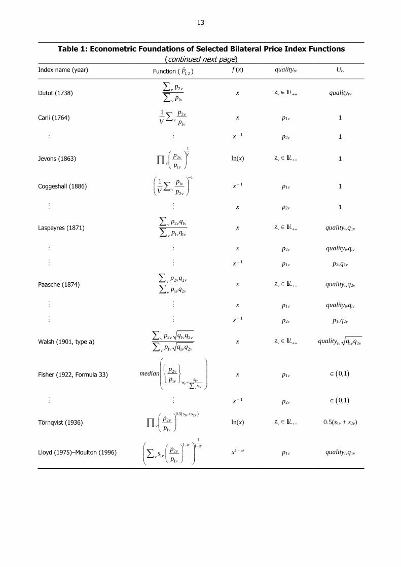
Table 1 lists some of the complying bilateral functions and their settings for f (x), {Utv}, and

{qualitytv}. Emphasis is on types that are most important to measurement practitioners, based on

my judgement and the results of a statistical agency survey in Stoevska (2008). The table also lists

some for their unusual forms. It omits types that are averages of others, such as a celebrated ‘ideal’

function from Fisher (1922, p 142 Formula 153).

13

Table 1: Econometric Foundations of Selected Bilateral Price Index Functions

(continued next page)

Index name (year) Function ( 1,2P̂ ) f (x) qualitytv Utv

Dutot (1738) 2

1

vv

vv

p

p

x vz qualitytv

Carli (1764) 2

1

1 v

vv

p

V p x p1v 1

x – 1 p2v 1

Jevons (1863)

1

2

1

Vv

vv

p

p

ln(x) vz 1

Coggeshall (1886)

1

1

2

1 v

vv

p

V p

x – 1 p1v 1

x p2v 1

Laspeyres (1871) 2 1

1 1

v vv

v vv

p q

p q

x vz qualitytvq1v

x p2v qualitytvqtv

x – 1 p1v p2vq1v

Paasche (1874) 2 2

1 2

v vv

v vv

p q

p q

x vz qualitytvq2v

x p1v qualitytvqtv

x – 1 p2v p1vq2v

Walsh (1901, type a) 2 1 2

1 1 2

v v vv

v v vv

p q q

p q q

x vz

1 2tv v vquality q q

Fisher (1922, Formula 33) 1

1

2

1 vv

vv

v

sv ws

pmedian

p

x p1v 0,1

x – 1 p2v 0,1

Törnqvist (1936)

1 20.5

2

1

v vs s

v

vv

p

p

ln(x) vz 0.5(s1v + s2v)

Lloyd (1975)–Moulton (1996)

11 1

21

1

vvv

v

ps

p

x1 – p1v qualitytvq1v

14

Table 1: Econometric Foundations of Selected Bilateral Price Index Functions

(continued)

Index name (year) Function ( 1,2P̂ ) f (x) qualitytv Utv

Sato (1976)–Vartia (1976) 2

1

SatoVartiavw

v

vv

p

p

ln(x) vz

1 2

1 2ln ln

v v

v v

s s

s s

Redding and Weinstein (2018)

11

12 2

1 1

V

v v

vv v

p s

p s

ln(x) 1

1tvs 1

ln(x) tv 1 2

1 2ln ln

v v

v v

s s

s s

Notes: The Dutot, Carli, Laspeyres, Paasche and Moulton attributions have all been taken on authority of Balk (2008); vz is

intended to mean that any strictly positive definitions of quality that are fixed across t, are admissible; v v

v w ymedian x

is

a weighted median of the items in set {xv}, using weights of yv (the notation is non-standard); the notation 0,1

reflects that in median- and mode-based functions, only one observation has a non-zero weight;

1

1 2 1 2

1 2 1 2ln ln ln ln

SatoVartia v v w wv w

v v w w

s s s sw

s s s s

; is a consumer elasticity of substitution; the index from Redding

and Weinstein (2018) is what the authors refer to as the ‘common goods’ index; tv is a time-varying preference parameter,

explained further in the original paper

Notice that many types correspond to several distinct combinations of f (x), {Utv}, and {qualitytv}.

To exhaustively list the combinations associated with each type is a difficult problem, left for future

work. The result of that work might be surprising. To illustrate, Appendix E includes a derivation

from Bert Balk (pers comm, 16 March 2018) that generates an unexpected combination for the Dutot

function. Knowing all of the combinations would help for comparing the merits of the functions,

because it would demonstrate the breadth of relevant measurement preferences for which each

function is exact.

Still, it is clear that at least some types cover every possible {qualitytv} that is fixed over t. This

quality-robust feature adds to their appeal. Otherwise the functions tend to gauge qualitytv through

relative prices. To gauge qualitytv like this is an objective choice.1

A notable exception for the way it gauges qualitytv is a static-population function from Redding and

Weinstein (2018). It uses expenditure shares and allows qualitytv to vary over t. Derived using the

economic approach, the function aims to measure cost of living changes under dynamic preferences.

Using expenditure to gauge product quality like this has strong parallels in the international trade

literature. (Notable examples are papers by Khandelwal (2010) and Feenstra and Romalis (2014)).

Work by von Auer (2014) outlines a so-called Generalised Unit Value Index Family, which is relevant

here as well. Using the framework of this paper, the Family members are functions for which

f (x) = x, {qualitytv} is fixed over t within varieties, and Utv = qualitytvqtv for all (t, v) pairs. (von Auer

introduced axioms for sensible quality definitions as well.) Examples in the table are the indices of

Paasche and Laspeyres. The Family is special because the implied quantity index is always the

1 For another application the 2008 System of National Accounts does list some relevant cases in which gauging quality

like this is not ideal (European Commission et al 2009, p 303).

15

growth in the number of units of equal interest, which, in turn, are just the amounts of transacted

quality. This is an intuitive, appealing feature, and one way to interpret official measures of output

growth in, for instance, Australia and the United Kingdom.

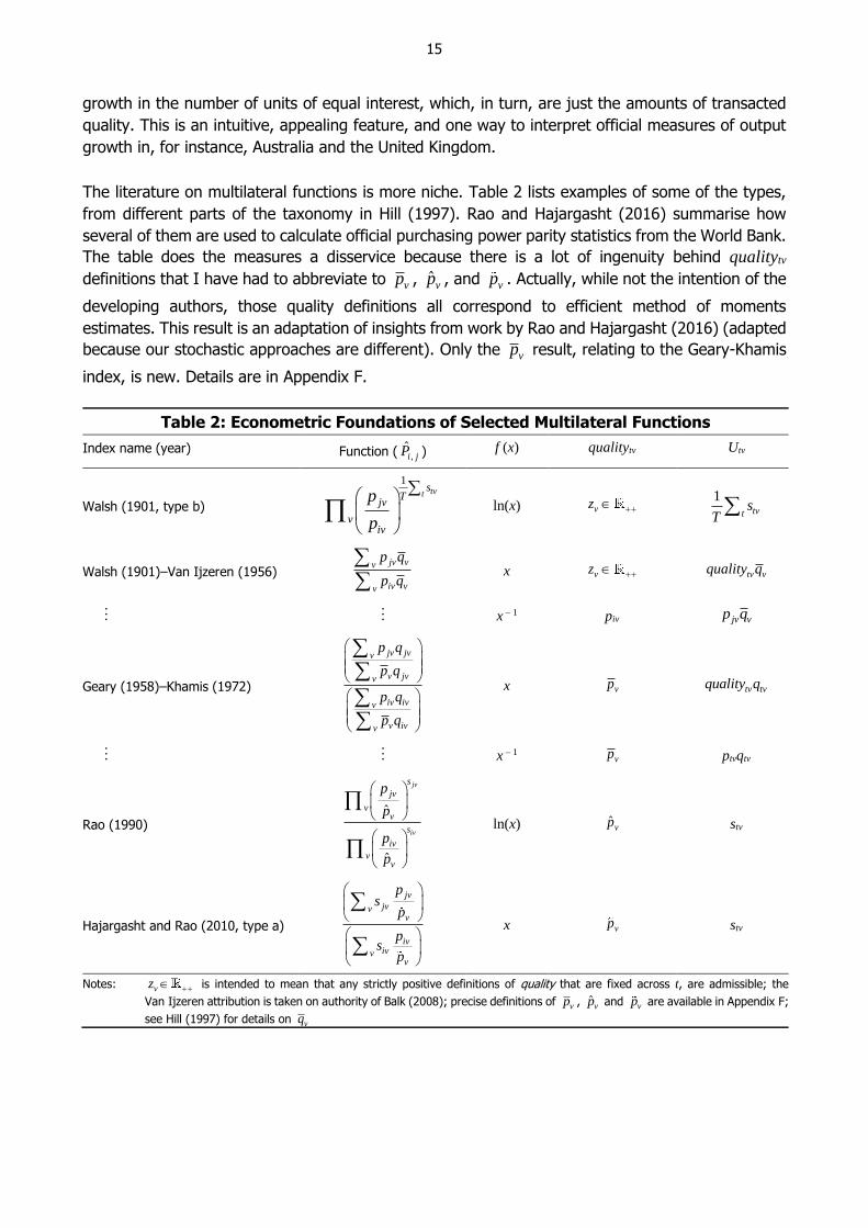
The literature on multilateral functions is more niche. Table 2 lists examples of some of the types,

from different parts of the taxonomy in Hill (1997). Rao and Hajargasht (2016) summarise how

several of them are used to calculate official purchasing power parity statistics from the World Bank.

The table does the measures a disservice because there is a lot of ingenuity behind qualitytv

definitions that I have had to abbreviate to vp , ˆvp , and vp . Actually, while not the intention of the

developing authors, those quality definitions all correspond to efficient method of moments

estimates. This result is an adaptation of insights from work by Rao and Hajargasht (2016) (adapted

because our stochastic approaches are different). Only the vp result, relating to the Geary-Khamis

index, is new. Details are in Appendix F.

Table 2: Econometric Foundations of Selected Multilateral Functions

Index name (year) Function ( ,ˆi jP ) f (x) qualitytv Utv

Walsh (1901, type b)

1tvt

sT

jv

viv

p

p

ln(x) vz 1

tvts

T

Walsh (1901)–Van Ijzeren (1956) jv vv

iv vv

p q

p q

x vz tv vquality q

x – 1 piv jv vp q

Geary (1958)–Khamis (1972)

jv jvv

v jvv

iv ivv

v ivv

p q

p q

p q

p q

x vp tv tvquality q

x – 1 vp ptvqtv

Rao (1990) ˆ

ˆ

jv

iv

s

jv

vv

s

iv

vv

p

p

p

p

ln(x) ˆvp stv

Hajargasht and Rao (2010, type a)

jv

jvvv

ivivv

v

ps

p

ps

p

x vp stv

Notes: vz is intended to mean that any strictly positive definitions of quality that are fixed across t, are admissible; the

Van Ijzeren attribution is taken on authority of Balk (2008); precise definitions of vp , ˆvp and vp are available in Appendix F;

see Hill (1997) for details on vq

16

3.3 This Changes the Stochastic Approach

Throughout this paper, measurement objectives have been defined using parameters from

econometric models. Econometric estimators have then justified the corresponding measurement

tools. When the population of varieties being transacted is static, the process is synonymous with

the stochastic approach to choosing index functions.

To date the stochastic approach has been less influential than the economic and test approaches. It

is actually more commonly used as an econometric gateway for generalising Jevons- and Törnqvist-

type functions to dynamic populations. Hence the widespread popularity of The Standard Model.

The approach has also been used as a means to calculate confidence intervals, to gauge index

reliability (see, for instance, Rao and Hajargasht (2016)).

Judging by Clements et al (2006), the lack of influence comes partly from reservations about the

stated econometric justifications for weighting. The occasional discomfort over weight endogeneity

has also mattered somewhat. Section 2 has shown that both objections are fair, but resolvable. The

econometric model just needs to define the parameters of interest carefully.

The new framework presented here has extended the approach in other ways as well:

The approach now has a wider scope. It covers practically all existing price index functions and

infinitely more. So it is a more complete tool for comparing them. A repercussion is that index

types formerly considered as stochastic-compatible are no longer special for that reason.

Albeit not always in a unique way, the approach now distinguishes index types by their conceptual

characteristics. Previously the approach distinguished types by somewhat arbitrary modelling

assumptions.

Being specified in terms of prices, rather than price ratios, there is no built-in need for static

populations that produce matched price pairs. The approach is hence a means to carry standard

index function perspectives over into dynamic populations. (Some compromises are necessary,

and will be discussed further in Section 4.2.)

The changes, in turn, provide an alternative means of understanding and communicating

measurement challenges to economic researchers that do not have specialist backgrounds in

measurement. Consider the phenomenon of chain drift, which occurs in index functions that provide

different results under chained comparisons than under direct ones (see Ivancic, Diewert and

Fox (2011)). The chained and direct indices imply different populations of interest, because they

have different units of equal interest. Using either set-up as the correct benchmark, the gap between

them can be viewed as reflecting endogeneity.

In some cases, the changes can also open new avenues for tackling measurement problems. The

next section discusses three examples, and some obvious avenues for further progress. As the

discussion is targeted at measurement specialists, applied macro researchers can skip comfortably

to the conclusion.

17

4. The New Framework Challenges Some Practices

4.1 The Goldberger (1968) Bias Correction is Unnecessary

For models with a semi-log form, like The Standard Model, the international consumer and producer

price index manuals recommend a bias correction for ˆ ˆj ie

(International Labour Office et al 2004,

p 118; International Labour Organization et al 2004, p 184). Following Goldberger (1968), the

correction is to account for the fact that

ˆ ˆ

ˆ ˆ j i j i

j i j i e e

(13)

The Diewert Model is also semi-log, so the same applies. The proposed bias-corrected estimator is

,ˆ ˆ ˆ ˆ ˆ ˆexp 0.5VarGoldbergeri j j i j iP (14)

where ˆVar is estimated variance. The correction matters most when the variance of ˆ ˆj i is

largest, which, in turn, is more likely for cases with small sample sizes and few controls. An empirical

illustration in Kennedy (1981) shows the correction to make a small difference. More measurement-

focused illustrations in Syed, Hill and Melser (2008) and de Haan (2017), show it to make a trivial

difference. However, these examples use large samples and many controls. As pointed out by

Hill (2011), we cannot rule out there being cases for which the correction is material.

But even in cases where the bias correction matters, is it sensible? Here I show that it seems to

imply incompatible analytical preferences.

With the t coming from a semi-log model, defining the measurement objective as ,j i

i jP e

is

just articulating that the preferred measure of central tendency is a geometric average. In particular,

taking a finite view of the population, which is a common choice in the measurement literature,

revealed preference is for a ratio comparison of

1 1

andjv ivv v

U U

juv iuv

uv uv

p p

(15)

For a more standard, continuous view of the population, the corresponding geometric-type averages

look more complicated. They are

exp ln and exp lnjuv juv iuv iuvp dF p p dF p (16)

where F(·) is a cumulative density function and the integrals are over u and v.

If interest is in geometric-type averages like these, why then would we subject ,ˆi jP to a standard

test of unbiasedness, which is an arithmetic criteria of central tendency? Logical consistency would

dictate the use of a compatible, geometric criteria.

18

It turns out that with a geometric criteria a correction is unnecessary. In particular,

ˆ ˆ

,ˆ ˆ ˆexp ln ,j igeometrici j i jP e dF

(17)

ˆ ˆexp j i (18)

j ie

(19)

,i jP (20)

where geometric is a geometric type of expectation operator and F(·,·) is a cumulative density

function.

The natural follow-up question is whether compatible criteria of central tendency always generate

such benign results. The answer: not necessarily.

To illustrate, let * denote an expectation operator that is logically consistent with the choice of

f (·), such that

1

, 1

ˆˆ* *

ˆ

OLSjgeneral

i j OLSi

fP

f

(21)

1

1

1

ˆˆ ˆ,

ˆ

OLSj

i jOLSi

ff f dF

f

(22)

Now let f (x) = x, where is a non-zero real number. Along with f (x) = x, this setting for f (x) covers

all of those that currently appear in the measurement literature. Denote the corresponding index

and target as ,ˆi jP and ,i jP . Generally it will be the case that

1

,

ˆˆ ˆ ˆ* ,

ˆ

OLSj

i j i jOLSi

P dF

(23)

1

ˆ

ˆ

OLSj

OLSi

(24)

1

j

i

(25)

19

,i jP (26)

There are, however, important special cases. In particular, many indices use definitions of quality

for which qualitytv = priceiuv for all t, u, and v. In that case it always holds that ˆ 1OLS OLSi i .

Hence

1

1 1

,

ˆˆ

ˆ

OLSj OLS

j j i jOLSi

P

(27)

This is an unusual result. It means that for indices like Paasche, interpretations that set

qualitytv = priceiuv are more achievable in small samples than other interpretations.

4.2 Some Dynamic Population Methods Look Questionable

In durable goods markets especially, the norm is for the population of transacted varieties to be

dynamic. Yet index functions, the primary tools of economic measurement, are designed for static

populations of varieties.

A crude workaround is to drop orphan varieties. However, the prevailing view in the field of

measurement is that orphan status is non-random. Dropping the orphans generates what is akin to

another endogenous sampling problem. More sophisticated methods are needed. According to

Triplett (2004, p 9), handling quality change that comes from a changing population has ‘long been

recognised as perhaps the most serious measurement problem in estimating price indexes’.

Moulton (2017) explains how successive investigations have estimated that the problem accounts

for the largest source of measurement bias in the US consumer price index.

The updated stochastic approach presented here offers a useful perspective on the problem. As

shown below, without any intrinsic dependence on price ratios, it provides avenues through which

to extend index function principles to dynamic populations. It is also a means to identify existing

dynamic population methods that are incompatible with the (stochastic approach) principles behind

index functions.

When extending to dynamic populations, not all of the features of index functions can be preserved,

and compromises are necessary:

Some choices of {qualitytv} become undefined. In particular, {qualitytv} cannot be benchmarked

to prices if some of them are missing from the population. In this case, the missing transaction

prices that are needed to fully define {qualitytv} might defensibly be viewed as having synthetic

values, each corresponding to what might have been the price had the variety been transacted.

In the estimation phase, coming up with these values is often called ‘patching’ or ‘imputing’. The

measurement literature already contains many approaches to patching (see International Labour

Office et al (2004), International Labour Organization et al (2004), and Eurostat (2013)).

20

Section 3.2 showed that, in static populations, some distinct combinations of f (x), {Utv}, and

{qualitytv} coincide with others. The same feature breaks down in dynamic populations. So

practitioners looking to generalise an index function to a dynamic population must choose just

one combination. Alternatively, they could choose several combinations, calculate a separate

index for each, and take an average. The latter approach is similar in spirit to, say, the ideal index

from Fisher (1922).

Strategies like these are already being used. For instance, when constructing an index directly from

a dynamic population version of The Standard Model, practitioners are implicitly choosing a single

definition for {qualitytv}, based on a least squares criteria. Using the method of moments approach

outlined in Rao and Hajargasht (2016) (examples are in Appendix F), a least squares criteria for

choosing {qualitytv} could be executed under all sorts of other settings for f (x) and {Utv}.

The literature contains criticisms of this direct method, which have stifled take-up by national

statistical offices. The key criticism is ultimately about the definition of quality. For instance, in 2002,

responding to a request by the US Bureau of Labor Statistics (BLS), a panel of experts wrote:

Recommendation 4-4: BLS should not allocate resources to the direct … method (unless work on other

hedonic methods generates empirical evidence that characteristic parameter stability exists for some

products). (National Research Council 2002, p 143)

The concern is that restricting the coefficients on variety specifications to be fixed over time is

unlikely to reflect the true conditional expectation function for prices. Several papers have rejected

parameter stability for the computer market in the United States (Berndt and Rappaport 2001;

Pakes 2003), and have echoed the panel’s recommendation (see also Diewert et al (2009) and

Hill (2011)).

Viewed through the updated stochastic approach, this argument looks problematic for two reasons:

The objection really is to fixing the quality definition across t, within varieties. Yet the same is

true of all common index numbers. If fixing each variety’s quality definition is indeed a drawback,

index function choices need to be reconsidered too. Functions with quality definitions that change

over t, like the common goods index from Redding and Weinstein (2018), would need to become

more mainstream.

To repeat a point made already, there is no need for the model to describe the conditional

expectation function exactly (i.e. requiring the errors to be strictly exogenous to the regressors).

It is sufficient for the model to identify useful descriptive statistics (i.e. accepting errors that are

only uncorrelated with the regressors).

Moreover, the proposed alternatives do not actually address the fixed quality problem. For instance,

the most popular alternative is to use synthetic values for all missing transaction prices, not just the

missing prices needed to define quality. Standard index functions can then be applied. However, no

matter where those synthetic values come from, the index functions that are typically applied to the

new population still take constant quality perspectives. Moreover, the interpretation of the final index

is no longer an average of quality-adjusted actual prices. Instead it is

21

,ˆ

juv juv

jv jvpatchedi j

iuv iuv

iv iv

p paverage

quality qualityP

p paverage

quality quality

(28)

where the juv indexes fictitious product observations, from the additional patching. The same

issue transfers to the population target. (Conditions under which the additional patching makes no

difference are provided in de Haan (2008).)

Diewert et al (2009) examine and propose another alternative, which they show is also equivalent

to the so-called characteristics prices method. The method is fully consistent with the new stochastic

approach presented in this paper, it being akin to calculating indices for several combinations of

f (x), {Utv}, and {qualitytv}, before taking an average. Still, the underlying quality definitions are

fixed over time.

Note that Feenstra (1994), Ueda, Watanabe and Watanabe (2016), and Redding and

Weinstein (2018) introduce other, deterministic methods to handle dynamic populations. The

methods do not seem to have obvious connections to the stochastic approach presented here, but

are justified by the economic approach.

Occasionally, the literature also defines dynamic population indices using models that are like The

Standard Model, except that the dependent price variable is in levels, rather than logs. Since this

set-up is obviously not a special case of Equation (8), it is also in conflict with the principles behind

the stochastic approach.

4.3 Unit Values Can Distort Index Number Interpretation

So far we have assumed that each (t, v) pair has a single price. The assumption is unrealistic in the

general case, even with fully efficient markets. For instance, each t is an area, not a point, in space

or time. A price shock can fall easily within its boundaries. How should measurement methods handle

breaches of the single price assumption?

Current practice, stemming from Walsh (1901), Fisher (1922) and Davies (1932), is to specify

measurement tools in terms of ‘unit values’ (see International Labour Office et al (2004) and

International Labour Organization et al (2004)). Regardless of the situation, the unit values are

always equal to the total measured expenditure on each (t, v) pair, divided by the number of units

transacted. That is, letting tuvp denote the unit value for pair (t, v),

tnvn

tuv

tv

pp

q

(29)

where the subscript n tracks each of the individual transactions. Unit values are hence quantity-

weighted, arithmetic averages of prices.

22

The attraction of the unit values solution is that it can shoehorn reality into the traditional formulation

of index functions. Moreover, it has low information requirements, needing only total expenditures

(numerator) and numbers of transactions (denominator) for each variety. But the functions – and

their population targets – are then comparing averages of quality-adjusted unit values at different

points in space or time. Are there sensible ways to preserve a cleaner interpretation, about quality-

adjusted raw prices? Would the outcomes even be different?

With its more flexible formulation, the new stochastic approach framework presented in this paper

is an avenue through which to tackle these questions. Diewert (2004) and Rao and

Hajargasht (2016) also noted the potential of stochastic approaches to handle raw prices if they are

available.

Preserving the raw prices interpretation requires only that, for each variety in a given time period,

the units of equal interest are allocated to the different transaction prices somehow. Since each of

the transactions for a variety are (definitionally) for a homogeneous product, it seems the only

sensible solution is to allocate units of equal interest in proportion to the number of transactions

executed at each price. Sometimes this will correspond to the unit values solution, but sometimes it

will not.

To illustrate, I will focus on index functions, rather than their population targets. The same ideas

carry over easily though.

Denote the index that uses raw prices as

1

,

1

1

ˆ

1

juv

uvjv jvvraw

i j

iuv

uviv ivv

pf f

U qualityP

pf f

U quality

(30)

and the one that uses unit values as

1

,

1

1

ˆ

1

juv

jvvjv jvvunitvalue

i j

iuvivv

iv ivv

pf U f

U qualityP

pf U f

U quality

(31)

The indices are equivalent if

,tuv tuvtv

u tv tv

p pf U f t v

quality quality

(32)

1 1

,tuvtv tuv

utv tv

pf f quality p t v

U quality

(33)

23

Letting f (x) = x, a common choice for many indices, the condition reduces to

1

,tuv tuv

utv

p p t vU

(34)

Now, use S to denote some strictly positive scalar, and allocate the units of equal interest evenly

across each transaction. The raw prices calculation on the left-hand side of Equation (34) becomes

1 1 1

,tuv tnv tnv

u n ntv tv tv

p Sp p t vU Sq q

(35)

The result does indeed correspond to the unit values solution on the right-hand side of Equation (34).

The unit value method looks ideal.

For other choices of f (x) the unit value method looks less benign. For instance, consider the choice

of f (x) = ln(x). Equivalence to the raw prices method is guaranteed only when

1

,tvUtuv tuv

u

p p t v (36)

If units of equal interest are allocated evenly across transactions, the raw prices solution on the left-

hand side becomes

1 1

,tv tv tv

S

U Sq qtuv tnv tnv

u n n

p p p t v (37)

Equivalence to the unit values method is unlikely to hold, since

11

,tvqtnv tnv

nn tv

p p t vq

(38)

When there is any variation in transaction prices for a given (t, v) pair, the inequality is strict

(Balk 2008, p 70).

So for some types of f (x), the unit value method necessarily changes the interpretation of the index,

or can be seen as distorting the true index. This should be unsurprising; the unit value method takes

a position on the appropriate measure of central tendency without considering the choice of f (x),

which is also a position on the appropriate measure of central tendency.

24

4.4 There Are Obvious Avenues for Further Progress

In establishing the new stochastic framework, and the results that come from it, this paper has left

many obvious questions unanswered:

Can we determine exactly how many distinct combinations of f (x), {Utv}, and {qualitytv}

correspond to each price index? And can we be precise about what those are? The answers would

be useful for comparing the merits of various functions. They might also yield new options for

handling dynamic populations.

Can we definitively rule out some indices from complying with the stated paradigm? If so, is this

a problem with the paradigm or the index?

What corrections are sensible for the measurement approaches that have undesirable central

tendencies in small samples? Would the corrections ever be material enough to promote for use

at national statistical offices?

How material in practice are the unit value distortions that I have identified?

What does the new framework imply for appropriate confidence intervals? Do the implications

align with existing work on index number uncertainty, such as Crompton (2000), Clements

et al (2006), and Rao and Hajargasht (2016)?

Should the same perspectives on the population of interest be incorporated elsewhere in the

empirical macro literature?

These are potentially fruitful subjects for future work. The final one is the topic of a forthcoming

paper. With time, the deeper connections to the econometric literature might reveal other

opportunities.

5. Conclusion

There is a material difference between modelling, say, the price of dwellings (distinct residences),

and the price of housing (the infrastructure providing shelter). Modelling the price of housing is a

more macro-oriented task and implies a synthetic population of interest. A simple way to implement

the macro orientation is to write the model in terms of what I call units of equal interest.

In the field of economic measurement it is common to model prices from macro perspectives, so

units of equal interest come up a lot. In fact this paper shows that practically all price index functions

are defined by their choice of average, their definition of quality, and their stance on equal interest.

For instance, the Törnqvist function, used in the official chained version of the US consumer price

index, is defined by the geometric average, any definitions of quality that are constant over adjacent

time periods, and units of equal interest that are proportional to expenditure shares. The Laspeyres

function, used in the Australian consumer price index, is defined by the arithmetic average,

definitions of quality that are proportional to (closing period) prices, and units of equal interest that

are proportional to transacted amounts of quality.

25

This new framework for differentiating between index functions is free of ambitious modelling

assumptions. Hence it is more defensible and conceptual than the so-called stochastic approaches

that preceeded it. By covering practically all index functions, it is also more comprehensive. And the

time investment needed to understand it is small. This hopefully makes it useful for other macro

researchers wanting to appreciate the strengths and weaknesses of the tools they are routinely

using.

For measurement specialists, the new framework might offer new avenues to understand and tackle

measurement problems. To illustrate, I use it to challenge the use of the Goldberger (1968) bias

correction, the widespread reliance on unit values, and some common views on quality adjustment

with dynamic populations. At a high level, this work is a stochastic complement to recent research

on the economic approach to index functions by Redding and Weinstein (2018), because it unifies a

wide range of measurement methods.

26

Appendix A: The Inconsistency Arising from Endogenous Weighting is a Linear Projection

Let and xtv be vector shorthand for the full set of coefficients and regressors that are implicit in

The Standard Model, for a given (t, v) pair. Then

1

ˆ lnWLStv tv tv tv tv tv

tv tv

w w p

δ x x x (A1)

1

1 1lntv tv tv tv tv tv

tv tv

w w pV V

x x x (A2)

Applying the Law of Large Numbers and the Continuous Mapping Theorem (see Hansen (2018)),

1

1

ˆplim ln

ˆplim

WLSV tv tv tv tv tv tv

WLSV tv tv tv tv tv tv

w w p

w w

δ x x x

δ δ x x x

(A3)

The right-hand side of Equation (A3) is a weighted linear projection of the errors on the regressors.

Since the weights are functions of errors, the second expectation term is not zero.

27

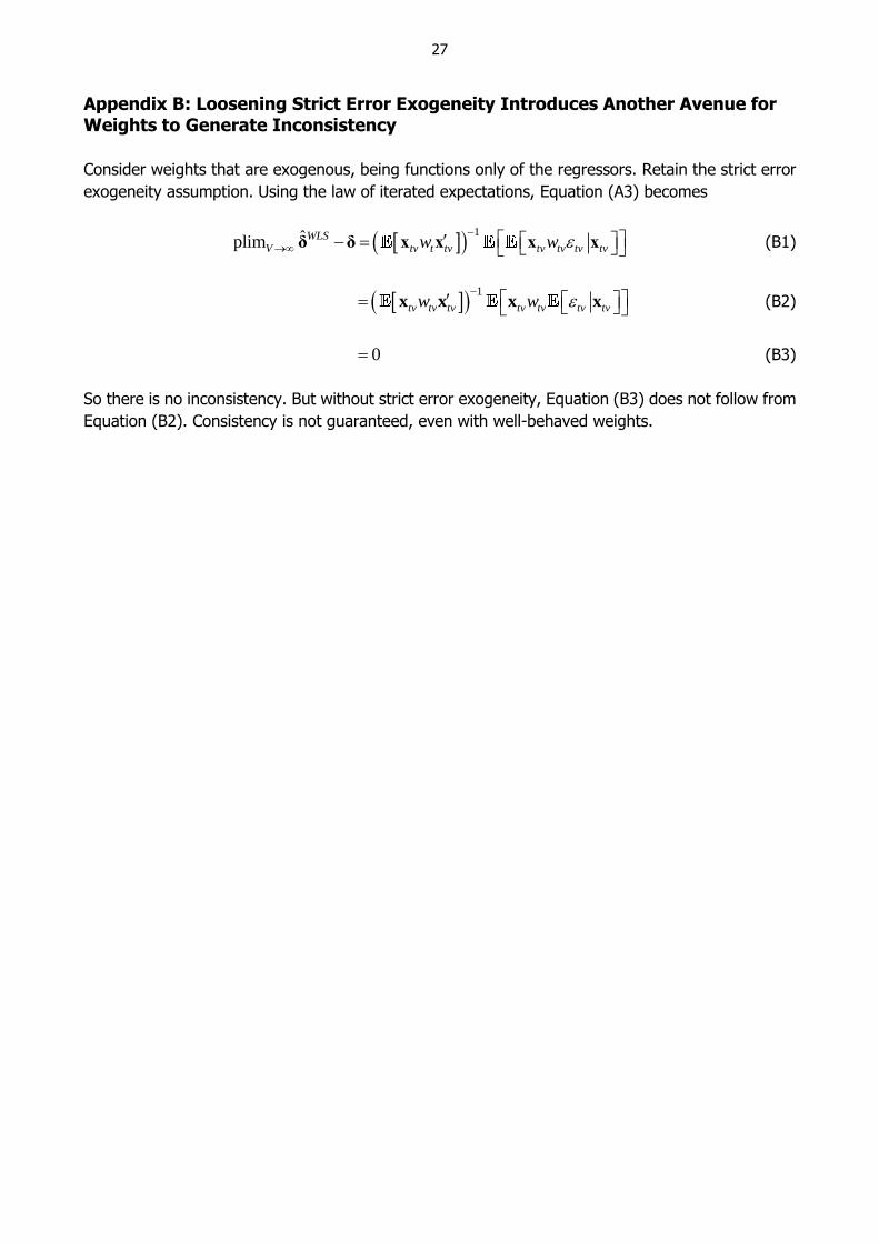
Appendix B: Loosening Strict Error Exogeneity Introduces Another Avenue for Weights to Generate Inconsistency

Consider weights that are exogenous, being functions only of the regressors. Retain the strict error

exogeneity assumption. Using the law of iterated expectations, Equation (A3) becomes

1ˆplim WLS

V tv t tv tv tv tv tvw w

δ δ x x x x (B1)

1

tv tv tv tv tv tv tvw w

x x x x (B2)

0 (B3)

So there is no inconsistency. But without strict error exogeneity, Equation (B3) does not follow from

Equation (B2). Consistency is not guaranteed, even with well-behaved weights.

28

Appendix C: The Model of Voltaire and Stack (1980) Equates to The Diewert Model, under Restrictive Conditions Only

Using my notation and making some trivial generalisations, the model of Voltaire and Stack (1980)

swaps A1’ for A1”.

A1”

* ln 1, , ; 1, , *tv tv t v tvV w p t T v V β spec (C1)

where V* is the number of varieties in a population viewed to be finite (as opposed to the more

common, superpopulation viewpoint).2

In the original application the population is static and wjv = wiv for all i and j. If also

/tv tv tvvw U U , as looks to be the intention, the model identifies the same j – i as the

equivalent case of The Diewert Model. Otherwise the relevance of the Voltaire and Stack model is

easy to break.

To illustrate, note that under the above conditions, for any i ≠ j, the key assumptions of the Voltaire

and Stack model can be rewritten in the form

* ln * lnv vjv iv j i jv iv

v vv v

U UV p V p

U U

(C2)

,*ln

v

vv

U

Ujv

i j jv iv

iv

pV

p

(C3)

and

0jv iv (C4)

Therefore

, *ln

v

vv

U

Ujv

i j

iv

pV

p

(C5)

Since the Voltaire and Stack model views the population as finite, with V* varieties,

2 The superpopulation viewpoint can encompass the finite population one, by conceptualising the population outcomes

as having discrete possibilities, with densities proportional to realised incidence.

29

1

*ln *ln*

v v

v vv v

U U

U Ujv jv

viv iv

p pV V

p V p

(C6)

ln

v

vv

U

Ujv

v iv

p

p

(C7)

Under the same conditions, The Diewert Model implies

ln lnjuv iuv j i iuv juvp p (C8)

,lnjuv

i j iuv juv

iuv

p

p

(C9)

where

0iuv juv (C10)

Taking the same finite perspective on the population,

, lnjuv

i j

iuv

p

p

(C11)

1

lnjv

tv

vv ivv

pU

U p

(C12)

ln

v

vv

U

Ujv

v iv

p

p

(C13)

which mirrors the result for the Voltaire and Stack model.

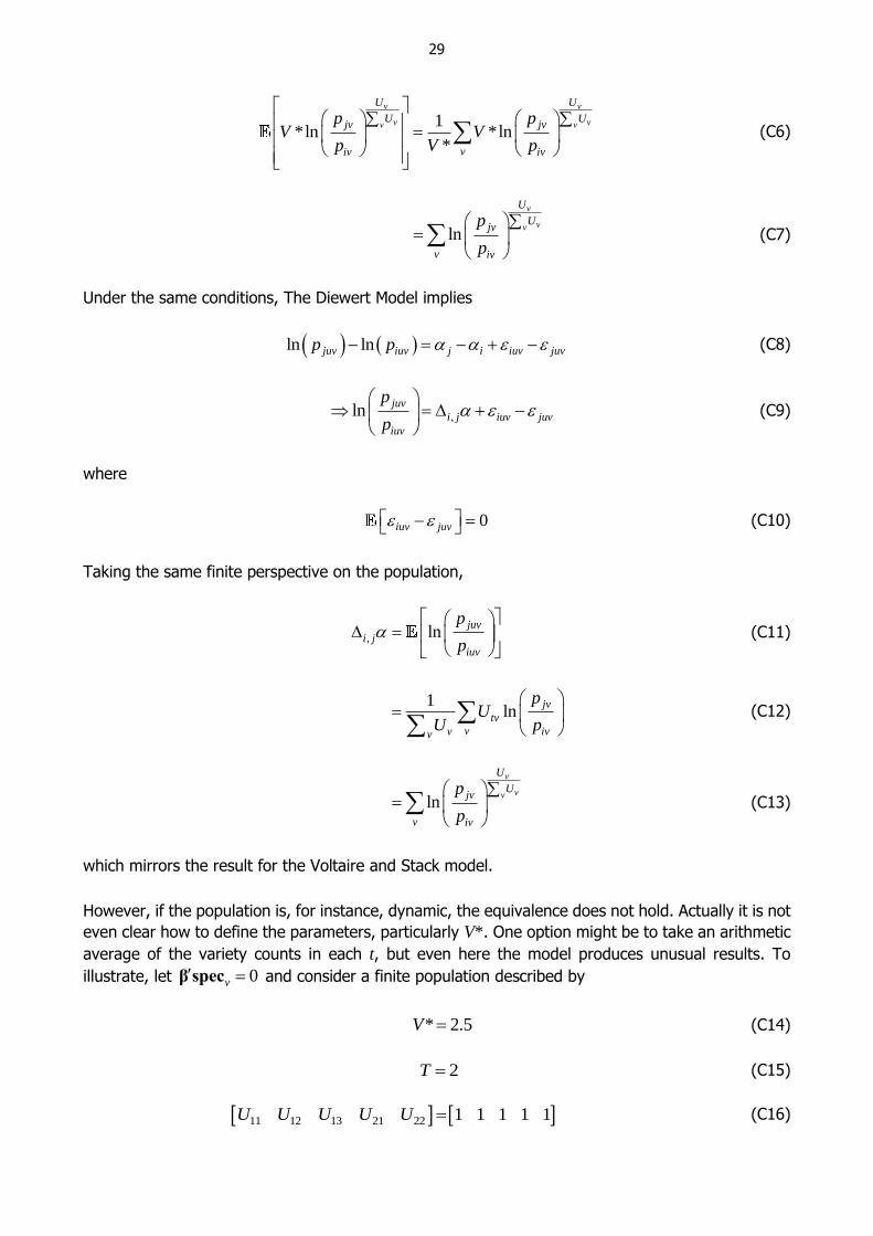
However, if the population is, for instance, dynamic, the equivalence does not hold. Actually it is not

even clear how to define the parameters, particularly V*. One option might be to take an arithmetic

average of the variety counts in each t, but even here the model produces unusual results. To

illustrate, let 0v β spec and consider a finite population described by

* 2.5V (C14)

2T (C15)

11 12 13 21 22 1 1 1 1 1U U U U U (C16)

30

11 12 13 21 22ln ln ln ln ln 5 6 7 6 8p p p p p (C17)

The Voltaire and Stack model identifies the parameters to be

1

1 1 12.5 5 2.5 6 2.5 7

3 3 3 53

(C18)

and

2

1 12.5 6 2.5 8

2 2 8.752

(C19)

These are nonsensical results, particularly the second, being outside the range of population prices

in t = 2. The equivalent figures for The Standard Model are 1 = 6 and 2 = 7.

The other drawback of the Voltaire and Stack model is its lack of conceptual appeal. The authors do

not justify the relevance of the dependant variable, so it is unclear why the coefficients are

interesting.

31

Appendix D: Some Choices of f (x), {Utv}, and {qualitytv} are Always Equivalent

In

1

,

1

1

1

juv

uvjv jvvgeneral

i j

iuv

uviv ivv

pg g

U qualityP

pg g

U quality

(D1)

let g(·) = A + Bf (·), where A and B are scalars.

Then

1

,

1

1

1

juv

uvjv jvv

generali j

iuv

uviv ivv

pA Bf A

U qualityf

B

Pp

A Bf AU quality

fB

(D2)

1

1

1

1

juv

uvjv jvv

iuv

uviv ivv

pf f

U quality

pf f

U quality

(D3)

So choosing any function f (·) is always equivalent to choosing any of its affine transformations

A + B(f (·)).

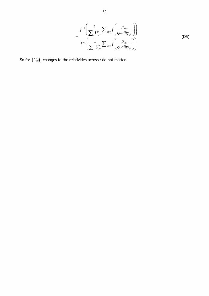
Now let iv ivU CU and jv ivU DU , where C and D are strictly positive scalars.

The identity in Equation (11) becomes

1

,

1

1

1

juv

u vjvjvvgeneral

i j

iuv

u vivivv

pf D f

qualityD UP

pf C f

qualityC U

(D4)

32

1

1

1

1

u v

juvjvjvv

iuv

u vivivv

pf f

qualityU

pf f

qualityU

(D5)

So for {Utv}, changes to the relativities across t do not matter.

33

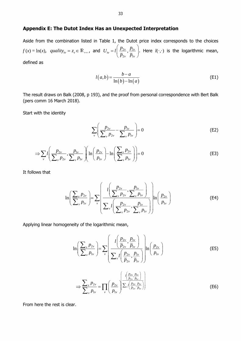
Appendix E: The Dutot Index Has an Unexpected Interpretation

Aside from the combination listed in Table 1, the Dutot price index corresponds to the choices

f (x) = ln(x), tv vquality z , and 2 1

2 1

,v vtv

v v

p pU l

p p

. Here l(·,·) is the logarithmic mean,

defined as

,ln ln

b al a b

b a

(E1)

The result draws on Balk (2008, p 193), and the proof from personal correspondence with Bert Balk

(pers comm 16 March 2018).

Start with the identity

2 1

2 1

0v v

v v vv v

p p

p p

(E2)

22 1 2

2 1 1 1

, ln ln 0vv v v v

v v v v vv v v

pp p pl

p p p p

(E3)

It follows that

2 1

2 12 2

1 12 1

2 1

,

ln ln

,

v v

v vv v vv v

vv vv v v

vv vv v

p pl

p pp p

p pp pl

p p

(E4)

Applying linear homogeneity of the logarithmic mean,

2 1

2 2 1 2

1 12 1

2 1

,

ln ln

,

v v

v v vv v

vv vv vvv

v v

p pl

p p p p

p pp pl

p p

(E5)

2 1

2 1

2 1

2 1

,

2 ,2

1 1

v v

v v

v vv

v v

p pl

p p

p pv lv vp p

vv vv

p p

p p

(E6)

From here the rest is clear.

34

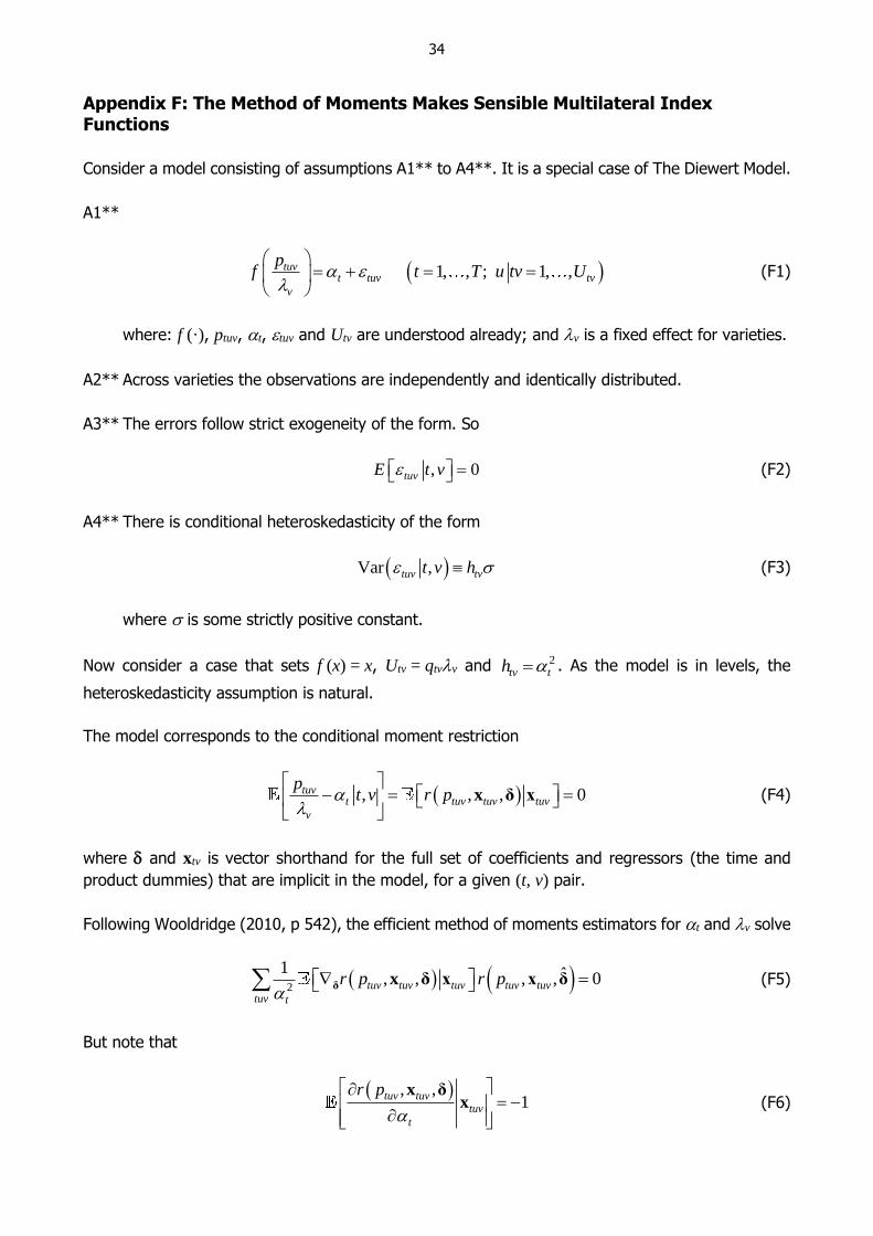
Appendix F: The Method of Moments Makes Sensible Multilateral Index Functions

Consider a model consisting of assumptions A1** to A4**. It is a special case of The Diewert Model.

A1**

1, , ; 1, ,tuvt tuv tv

v

pf t T u tv U

(F1)

where: f (·), ptuv, t, tuv and Utv are understood already; and v is a fixed effect for varieties.

A2** Across varieties the observations are independently and identically distributed.

A3** The errors follow strict exogeneity of the form. So

, 0tuvE t v (F2)

A4** There is conditional heteroskedasticity of the form

Var ,tuv tvt v h (F3)

where is some strictly positive constant.

Now consider a case that sets f (x) = x, Utv = qtvv and 2tv th . As the model is in levels, the

heteroskedasticity assumption is natural.

The model corresponds to the conditional moment restriction

, , , 0tuvt tuv tuv tuv

v

pt v r p

x δ x (F4)

where and xtv is vector shorthand for the full set of coefficients and regressors (the time and

product dummies) that are implicit in the model, for a given (t, v) pair.

Following Wooldridge (2010, p 542), the efficient method of moments estimators for t and v solve

2

1 ˆ, , , , 0tuv tuv tuv tuv tuv

tuv t

r p r p

δ x δ x x δ (F5)

But note that

, ,

1tuv tuv

tuv

t

r p

x δx (F6)

35

and

2

, ,tuv tuv tuv ttuv tuv

v vv

r p p

x δx x (F7)

the last of which contains the unknown parameters and . The feasible method of moments

estimators use ̂ and ̂ instead.

The resulting system of equations is

ˆˆˆ 0

ˆˆ

tv tv

ttv tv t

t v

t t tvv t

p q

q pv v

q

(F8)

and

ˆ ˆ ˆ0ˆ ˆ

tv tvtv vtv v t t

v v tv vv

p qpq t t

q

(F9)

This is the same as the system of Geary (1958) and Khamis (1972). The result differs somewhat

from the original method of moments derivation of Rao and Hajargasht (2016), who argue that an

inefficient weighting system is necessary to generate the index. Although our set-ups are different,

ultimately it is the introduction of units of equal interest that resolves the discrepancy.

Table F1 provides the settings needed to generate the other multilateral indices considered in Rao

and Hajargasht (2016), using the method of moments. I have not explored whether there are further

multilateral indices that fit the method of moments interpretation.

36

Table F1: Methods of Moments Interpretations of Multilateral Functions

Index name (year) 1 ˆ ,t vf f (x) Utv htv

Dutot-style 1

,tvv tv

tv tv

p p

T

x v

2t

Harmonic

1 1

1 1 1,v

v ttv t tvV p T p

x–1 1

2t

Geometric

11

,exp

TVtv tv

v tv t

p p

ln(x) 1 1

Geary (1958)–Khamis (1972) ,

tv tv

ttv tv tv

v tv tvv t

p q

p q

q q

x vqtv

2t

Iklé (1972)

1 1

1,v

tv tvv ttv t tv

s sp p

x–1 ptvqtv

2t

Rao (1990)

,exp

tvtvss

tv tv

v tv t

p p

ln(x) ptvqtv 1

Hajargasht and Rao (2010, type a) ,tv tvtv tvv t

v t

p ps s

x ptvqtv 2t

Hajargasht and Rao (2010, type b) 1 1

,tv tv

v tv t

p p

V T

x 1 2t

37

References

Australian Bureau of Statistics (2005), ‘The Introduction of Hedonic Price Indexes for Personal

Computers’, Information paper, ABS Cat No 6458.0.

Balk BM (2008), Price and Quantity Index Numbers: Models for Measuring Aggregate Change and

Difference, Cambridge University Press, Cambridge.

Banerjee KS (1983), ‘On the Existence of Infinitely Many Ideal Log-Change Index Numbers Associated with

the CES Preference Ordering’, Statistische Hefte, 24(1), pp 141–148.

Berndt ER (1991), The Practice of Econometrics: Classic and Contemporary, Addison-Wesley, Reading.

Berndt ER and NJ Rappaport (2001), ‘Price and Quality of Desktop and Mobile Personal Computers: A

Quarter-Century Historical Overview’, The American Economic Review, 91(2), pp 268–273.

Berry S, J Levinsohn and A Pakes (1995), ‘Automobile Prices in Market Equilibrium’, Econometrica, 63(4),

pp 841–890.

Brachinger HW, M Beer and O Schöni (2018), ‘A Formal Framework for Hedonic Elementary Price

Indices’, AStA Advances in Statistical Analysis, 102(1), pp 67–93.

Bryan MF and SG Cecchetti (1994), ‘Measuring Core Inflation’, in NG Mankiw (ed), Monetary Policy, NBER

Studies in Business Cycles, Vol 29, The University of Chicago Press, Chicago, pp 195–215.

Bureau of Labor Statistics (2017), ‘Quality Adjustment in the CPI’, viewed 11 February 2018. Available at

<https://www.bls.gov/cpi/quality-adjustment/home.htm>.

Bureau of Labor Statistics (2018), ‘Chapter 17. The Consumer Price Index’, Handbook of Methods,

rev 14 February 2018, Bureau of Labor Statistics, Washington DC, viewed 16 February 2018. Available at

<https://www.bls.gov/opub/hom/pdf/homch17.pdf>.

Clements KW and HY Izan (1981), ‘A Note on Estimating Divisia Index Numbers’, International Economic

Review, 22(3), pp 745–747.

Clements KW and HY Izan (1987), ‘The Measurement of Inflation: A Stochastic Approach’, Journal of

Business & Economic Statistics, 5(3), pp 339–350.

Clements KW, HY Izan and EA Selvanathan (2006), ‘Stochastic Index Numbers: A Review’, International

Statistical Review, 74(2), pp 235–270.

Coggeshall F (1886), ‘The Arithmetic, Geometric, and Harmonic Means’, The Quarterly Journal of

Economics, 1(1), pp 83–86.

Court AT (1939), ‘Hedonic Price Indexes with Automotive Examples’, The Dynamics of Automobile Demand,

General Motors Corporation, New York, pp 98–117.

Crompton P (2000), ‘Extending the Stochastic Approach to Index Numbers’, Applied Economics Letters,

7(6), pp 367–371.

38

Davies GR (1932), ‘Index Numbers in Mathematical Economics’, Journal of the American Statistical

Association, 27(177A), pp 58–64.

de Haan J (2004), ‘Hedonic Regression: The Time Dummy Index as a Special Case of the Imputation

Törnqvist Index’, Paper presented at the 8th Ottawa Group Meeting on Price Indices, Helsinki, 23–25 August.

de Haan J (2008), ‘Hedonic Price Indexes: A Comparison of Imputation, Time Dummy and Other

Approaches’, University of New South Wales, Centre for Applied Economic Research Working Paper 2008/01.

de Haan J (2017), ‘A Note on Bias Adjustment of the Time Dummy Hedonic Index’, Background paper

prepared for the Centre for Applied Economic Research EMG Workshop 2017, Sydney, 1 December.

de Haan J and F Krsinich (forthcoming), ‘Time Dummy Hedonic and Quality-Adjusted Unit Value Indexes:

Do They Really Differ?’, The Review of Income and Wealth.

de Haan J and HA van der Grient (2011), ‘Eliminating Chain Drift in Price Indexes Based on Scanner Data’,

Journal of Econometrics, 161(1), pp 36–46.

Diewert WE (1976), ‘Exact and Superlative Index Numbers’, Journal of Econometrics, 4(2), pp 115–145.

Diewert WE (1981), ‘The Economic Theory of Index Numbers: A Survey’, in A Deaton (ed), Essays in the

Theory of Consumer Behaviour: In Honour of Sir Richard Stone, Cambridge University Press, Cambridge,

pp 163–208.

Diewert WE (1992), ‘Fisher Ideal Output, Input, and Productivity Indexes Revisited’, Journal of Productivity

Analysis, 3(3), pp 211–248.

Diewert WE (2004), ‘On the Stochastic Approach to Linking the Regions in the ICP’, University of British

Columbia, Department of Economics Discussion Paper No 04-16. Available at

<https://econ.sites.olt.ubc.ca/files/2013/06/pdf_paper_erwin-diewert-notes-stochastic-approach.pdf>.

Diewert WE (2005), ‘Adjacent Period Dummy Variable Hedonic Regressions and Bilateral Index Number

Theory’, Annales d’Économie et de Statistique, 79/80, pp 759–786.

Diewert WE (2010), ‘On the Stochastic Approach to Index Numbers’, in WE Diewert, BM Balk, D Fixler,

KJ Fox and AO Nakamura (eds), Price and Productivity Measurement: Volume 6 - Index Number Theory,

Trafford Press, Bloomington, pp 235–262.

Diewert WE, S Heravi and M Silver (2009), ‘Hedonic Imputation versus Time Dummy Hedonic Indexes’,

in WE Diewert, JS Greenlees and CR Hulten (eds), Price Index Concepts and Measurement, NBER Studies in

Income and Wealth, Vol 70, University of Chicago Press, Chicago, pp 161–196.

Divisia F (1926), ‘L’indice Monétaire et la Théorie de la Monnaie (Suite et Fin)’ (The Monetary Index and the

Theory of Currency (Conclusion)), Revue d’Economie Politique, 40(1), pp 49–81.

European Commission, International Monetary Fund, Organisation for Economic Co-operation

and Development, United Nations and the World Bank (2009), System of National Accounts, 2008,

United Nations, New York.

39

Eurostat (2013), Handbook on Residential Property Price Indices (RPPIs), Methodologies and Working

Papers, Under the joint responsibility of the International Labour Organization, International Monetary Fund,

Organisation for Economic Co-operation and Development, Statistical Office of the European Union, United

Nations Economic Commission for Europe and the World Bank, European Union, Luxembourg.

Feenstra RC (1994), ‘New Product Varieties and the Measurement of International Prices’, The American

Economic Review, 84(1), pp 157–177.

Feenstra RC (1995), ‘Exact Hedonic Price Indexes’, The Review of Economics and Statistics, 77(4),

pp 634–653.

Feenstra RC and J Romalis (2014), ‘International Prices and Endogenous Quality’, The Quarterly Journal

of Economics, 129(2), pp 477–527.

Feenstra RC and MD Shapiro (2003), ‘High-Frequency Substitution and the Measurement of Price

Indexes’, in RC Feenstra and MD Shapiro (eds), Scanner Data and Price Indexes, NBER Studies in Income and

Wealth, Vol 64, University of Chicago Press, Chicago, pp 123–146.

Fisher I (1922), The Making of Index Numbers: A Study of Their Varieties, Tests, and Reliability, Publications

of the Pollak Foundation for Economic Research, No 1, Houghton Mifflin Company, Boston.

Fodor J and M Roubens (1995), ‘On Meaningfulness of Means’, Journal of Computational and Applied

Mathematics, 64(1–2), pp 103–115.

Fox KJ and IA Syed (2016), ‘Price Discounts and the Measurement of Inflation’, Journal of Econometrics,

191(2), pp 398–406.

Gábor-Tóth E and P Vermeulen (2017), ‘The Relative Importance of Taste Shocks and Price Movements

in the Variation of Cost-of-Living: Evidence from Scanner Data’, Paper presented at the 15th Ottawa Group

Meeting on Price Indices, Eltville am Rhein, 10–12 May.

Geary RC (1958), ‘A Note on the Comparison of Exchange Rates and Purchasing Power between Countries’,

Journal of the Royal Statistical Society: Series A (General), 121(1), pp 97–99.

German Federal Statistical Office (Statistisches Bundesamt) (2003), ‘Hedonic Methods of Price

Measurement for Used Cars’, Information paper, 20 October. Available at

<https://www.destatis.de/EN/FactsFigures/NationalEconomyEnvironment/Prices/HedonicUsedCars.pdf%3F_

_blob%3DpublicationFile>.

Goldberger AS (1968), ‘The Interpretation and Estimation of Cobb-Douglas Functions’, Econometrica,

36(3/4), pp 464–472.

Griliches Z (1971), ‘Introduction: Hedonic Price Indexes Revisited’, in Z Griliches (ed), Price Indexes and

Quality Change: Studies in New Methods of Measurement, Harvard University Press, Cambridge, pp 3–15.

Hajargasht G and DSP Rao (2010), ‘Stochastic Approach to Index Numbers for Multilateral Price

Comparisons and Their Standard Errors’, The Review of Income and Wealth, 56(S1), pp S32–S58.

Hansen BE (2018), ‘Econometrics’, Unpublished manuscript, University of Wisconsin, rev January. Available

at <https://www.ssc.wisc.edu/~bhansen/econometrics/Econometrics.pdf>.

40

Heravi S and M Silver (2007), ‘Different Approaches to Estimating Hedonic Indexes’, in ER Berndt and

CR Hulten (eds), Hard-to-Measure Goods and Services: Essays in Honor of Zvi Griliches, NBER Studies in

Income and Wealth, Vol 67, University of Chicago Press, Chicago, pp 235–268.

Hill RJ (1997), ‘A Taxonomy of Multilateral Methods for Making International Comparisons of Prices and

Quantities’, The Review of Income and Wealth, 43(1), pp 49–69.

Hill RJ (2011), ‘Hedonic Price Indexes for Housing’, OECD Statistics Working Paper No 2011/01.

Iklé DM (1972), ‘A New Approach to the Index Number Problem’, The Quarterly Journal of Economics, 86(2),

pp 188–211.

International Labour Office, International Monetary Fund, Organisation for Economic

Co-operation and Development, Statistical Office of the European Communities, United Nations

Economic Commission for Europe and the World Bank (2004), Consumer Price Index Manual: Theory

and Practice, International Labour Office, Geneva.

International Labour Organization, International Monetary Fund, Organisation for Economic

Co-operation and Development, United Nations Economic Commission for Europe and the

World Bank (2004), Producer Price Index Manual: Theory and Practice, International Monetary Fund,

Washington DC.

Ivancic L, WE Diewert and KJ Fox (2011), ‘Scanner Data, Time Aggregation and the Construction of Price

Indexes’, Journal of Econometrics, 161(1), pp 24– 35.

Jaimovich N, S Rebelo and A Wong (2015), ‘Trading Down and the Business Cycle’, NBER Working Paper

No 21539, rev October 2017.

Jevons WS (1863), A Serious Fall in the Value of Gold Ascertained, and Its Social Effects Set Forth,

Edward Stanford, London.

Jevons WS (1869), ‘Miscellanea: The Depreciation of Gold, 1847-69’, Journal of the Statistical Society of

London, 32(4), pp 445–449.

Kennedy PE (1981), ‘Estimation with Correctly Interpreted Dummy Variables in Semilogarithmic Equations’,

The American Economic Review, 71(4), p 801.

Keynes JM (1930), A Treatise on Money: Volume 1 The Pure Theory of Money, Macmillan and Co. Limited,

London.

Khamis SH (1972), ‘A New System of Index Numbers for National and International Purposes’, Journal of

the Royal Statistical Society: Series A (General), 135(1), pp 96–121.

Khandelwal A (2010), ‘The Long and Short (of) Quality Ladders’, The Review of Economic Studies, 77(4),

pp 1450–1476.

Kloek T and GM de Wit (1961), ‘Best Linear and Best Linear Unbiased Index Numbers’, Econometrica,

29(4), pp 602–616.

41

Lloyd PJ (1975), ‘Substitution Effects and Biases in Nontrue Price Indices’, The American Economic Review,

65(3), pp 301–313.

Machado JA and JMC Santos Silva (2006), ‘A Note on Identification with Averaged Data’, Econometric

Theory, 22(3), pp 537–541.

Montgomery JK (1937), The Mathematical Problem of the Price Index, P.S. King & Son, London.

Moulton B (2017), ‘The Measurement of Output, Prices, and Productivity: What’s Changed since the Boskin

Commission?’, Unpublished manuscript, November.

Nagumo M (1930), ‘Über eine Klasse der Mittelwerte’ (Over a Class of Means), Japanese Journal of

Mathematics: Transactions and Abstracts, 7, pp 71–79.

National Research Council (2002), At What Price?: Conceptualizing and Measuring Cost-of-Living and

Price Indexes, National Academy Press, Washington DC.

Office for National Statistics (2014), Consumer Price Indices Technical Manual: 2014 Edition, Office for

National Statistics, Newport.

Pakes A (2003), ‘A Reconsideration of Hedonic Price Indexes with an Application to PC’s’, The American

Economic Review, 93(5), pp 1578–1596.

Persons WM (1928), ‘The Effect of Correlation between Weights and Relatives in the Construction of Index

Numbers’, The Review of Economics and Statistics, 10(2), pp 80–107.

Rao DSP (1990), ‘A System of Log-Change Index Numbers for Multilateral Comparisons’, in J Salazar-Carrillo

and DSP Rao (eds), Comparisons of Prices and Real Products in Latin America, Contributions to Economic

Analysis, Vol 194, Elsevier Science Publishers B.V., Amsterdam, pp 127–139.

Rao DSP and G Hajargasht (2016), ‘Stochastic Approach to Computation of Purchasing Power Parities in

the International Comparison Program (ICP)’, Journal of Econometrics, 191(2), pp 414–425.

Redding SJ and DE Weinstein (2018), ‘Measuring Aggregate Price Indexes with Demand Shocks: Theory

and Evidence for CES Preferences’, NBER Working Paper No 22479, rev May.

Rosen S (1974), ‘Hedonic Prices and Implicit Markets: Product Differentiation in Pure Competition’, Journal

of Political Economy, 82(1), pp 34–55.

Sato K (1974), ‘Ideal Index Numbers that Almost Satisfy the Factor Reversal Test’, The Review of Economics

and Statistics, 56(4), pp 549–552.

Sato K (1976), ‘The Ideal Log-Change Index Number’, The Review of Economics and Statistics, 58(2),

pp 223–228.

Selvanathan E and DSP Rao (1994), Index Numbers: A Stochastic Approach, The Macmillan Press Ltd,

London.

Solon G, SJ Haider and JM Wooldridge (2015), ‘What Are We Weighting For?’, The Journal of Human

Resources, 50(2), pp 301–316.

42

Stoevska V (2008), ‘Consumer Price Index Manual: Theory and Practice – Report on the 2007 Worldwide

Survey on the Usefulness of the CPI Manual’, Report, International Labour Organization. Available at

<http://www.ilo.org/public/english/bureau/stat/download/cpi/survey.pdf>.

Stuvel G (1957), ‘A New Index Number Formula’, Econometrica, 25(1), pp 123–131.

Syed I, RJ Hill and D Melser (2008), ‘Flexible Spatial and Temporal Hedonic Price Indexes for Housing in

the Presence of Missing Data’, University of New South Wales, School of Economics Discussion Paper 08-14.

Available at <https://ideas.repec.org/p/swe/wpaper/2008-14.html>.

Theil H (1960), ‘Best Linear Index Numbers of Prices and Quantities’, Econometrica, 28(2), pp 464–480.

Theil H (1967), Economics and Information Theory, Studies in Mathematical and Managerial Economics,

Vol 7, North Holland Publishing Company, Amsterdam.

Törnqvist L (1936), ‘The Bank of Finland’s Consumption Price Index’, Bank of Finland Monthly Bulletin,

16(10), pp 27–34.

Triplett J (2004), Handbook on Hedonic Indexes and Quality Adjustments in Price Indexes: Special

Application to Information Technology Products, OECD Publishing, Paris.

Ueda K, K Watanabe and T Watanabe (2016), ‘Product Turnover and Deflation: Evidence from Japan’,

Australian National University, Crawford School of Public Policy, Centre for Applied Macroeconomics Analysis,

CAMA Working Paper 71/2016.

Vartia YO (1976), ‘Ideal Log-Change Index Numbers’, Scandinavian Journal of Statistics, 3(3), pp 121–126.

Voltaire K and EJ Stack (1980), ‘A Divisia Version of the Country-Product-Dummy Method’, Economics

Letters, 5(1), pp 97–99.

von Auer L (2014), ‘The Generalized Unit Value Index Family’, The Review of Income and Wealth, 60(4),

pp 843–861.

Walsh CM (1901), The Measurement of General Exchange-Value, The Macmillan Company, New York.

Wooldridge JM (2010), Econometric Analysis of Cross Section and Panel Data, 2nd edn, MIT Press,

Cambridge.

World Bank (2013), Measuring the Real Size of the World Economy: The Framework, Methodology, and

Results of the International Comparison Program—ICP, World Bank, Washington DC.