econometric methods of program evaluation manuel …arellano/ief-evaluation-marellano-tr.pdf ·...

Econometric Methods of Program EvaluationManuel Arellano

Cursos de Economía Pública del Instituto de Estudios FiscalesMadrid, 14 December 2010

I. Structural and treatment effect approaches

• The classic approach to quantitative policy evaluation in economics is the structuralapproach.

• Its goals are to specify a class of theory-based models of individual choice, choosethe one within the class that best fits the data, and use it for ex-post or ex-ante policysimulation.

• During the last two decades the treatment effect approach has established itself asa formidable competitor that has introduced a different language, different priorities,techniques and practices in applied work.

• Not only that, it has also changed the perception of evidence-based economics amongeconomists, public opinion, and policy makers.

• The ambition in a structural exercise is to use data from a particular context to identify,with the help of theory, deep rules of behavior that can be extrapolated to other contexts.

• A treatment effect (TE) exercise is context-specific and addresses less ambitious policyquestions.

• The goal is to evaluate the impact of an existing policy by comparing the distributionof a chosen outcome variable for individuals affected by the policy (treatment group)with the distribution of unaffected individuals (control group).

• The aim is to choose the control and treatment groups in such a way that membershipof one or the other, either results from randomization or can be regarded as if they werethe result of randomization.

• In this way one hopes to achieve the standards of empirical credibility on causal evi-dence that are typical of experimental biomedical studies.

2

• The TE literature has expressed dissatisfaction with the existing structural approachalong several dimensions:(a) Between theory, data, and estimable structural models there is a host of untestable

functional form assumptions that undermine the force of structural evidence by:(i) Having unknown implications for results.(ii) Giving researchers too much discretion.(iii) Complexity affects transparency and replicability.

(b) By being too ambitious on the policy questions we get very little credible evidencefrom data. Too much emphasis on ‘‘external validity’’ at the expense of the morebasic ‘‘internal validity’’.

• The TE literature sees the role of empirical findings as one of providing bits and piecesof hard evidence that can help the assessment of future policies in an informal way.

• Main gains in empirical research are not expected to come from the use of formaltheory or sophisticated econometrics, but from understanding the sources of variationin data with the objective of identifying policy parameters.

3

• Many policy interventions at the micro level have been evaluated:(a) training programs(b) welfare programs (e.g. unemployment insurance, worker’s sickness compensation)(c) wage subsidies and minimum wage laws(d) tax-credit programs(e) effects of taxes on labor supply and investment(f) effects of Medicaid on health

• I will review the following contexts or research designs of evaluation:(a) social experiments(b) matching(c) instrumental variables(d) regression discontinuity(e) differences in differences

• I pay special attention to instrumental-variable methods and their connections witheconometric models.

4

Descriptive analysis vs. causal inference

• It is useful to distinguish between descriptive analysis and causal inference as twotypes of micro empirical research.

• Their boundaries overlap, but there are good examples clearly placed in each category.

• Their difference is not in the sophistication of the statistical techniques employed.Sometimes the term ‘‘descriptive’’ is associated with tables of means or correlations,whereas terms like ‘‘econometric’’ or ‘‘rigorous’’ are reserved for regression coeffi-cients or more complex statistics of the same style.

• A simple comparison of means can be causal, whereas complex statistical analyses(like semiparametric censored quantile regression) can be descriptive.

• Perhaps the greatest successes of econometrics are descriptive analyses.

• Recent examples include trends in inequality and wage mobility, productivity mea-surement, or quality-adjusted inflation hedonic indices.

• A useful description is not a mechanical exercise. It is a valuable research activity,often associated with innovative ideas. The ideas have to do with the choice of aspectsto describe, the way of doing it, and their interpretation.

5

II. Potential outcomes and causality

• Association and causation have always been known to be different, but a mathematicalframework for an unambiguous characterization of statistical causal effects is surpris-ingly recent (Rubin, 1974; despite precedents in statistics and economics, Neyman,1923; Roy, 1951).

• Think of a population of individuals that are susceptible of treatment. Let Y1 be theoutcome for an individual if exposed to treatment and let Y0 be the outcome for thesame individual if not exposed. The treatment effect for that individual is Y1 − Y0.

• In general, individuals differ in how much they gain from treatment, so that we canimagine a distribution of gains over the population with mean

αATE = E (Y1 − Y0) .• The average treatment effect so defined is a standard measure of the causal effect of

treatment 1 relative to treatment 0 on the chosen outcome.

• Suppose that treatment has been administered to a fraction of the population, and weobserve whether an individual has been treated or not (D = 1 or 0) and the person’soutcome Y . Thus, we are observing Y1 for the treated and Y0 for the rest:

Y = (1−D)Y0 +DY1.

6

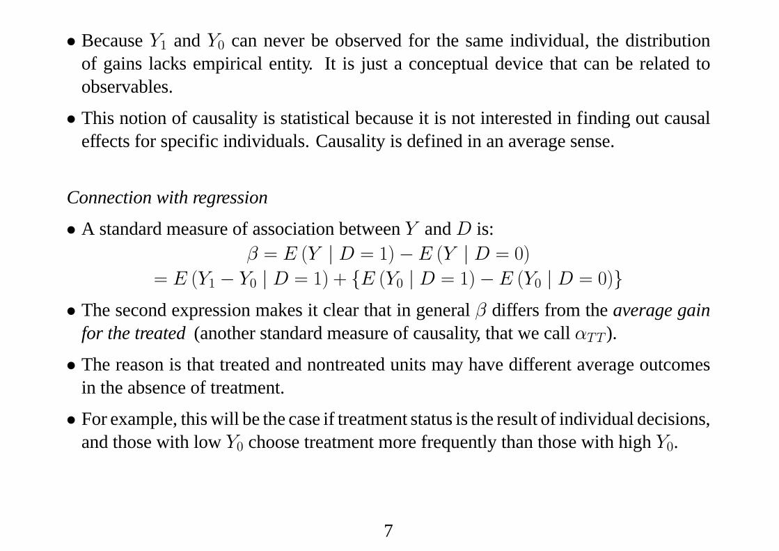
• Because Y1 and Y0 can never be observed for the same individual, the distributionof gains lacks empirical entity. It is just a conceptual device that can be related toobservables.

• This notion of causality is statistical because it is not interested in finding out causaleffects for specific individuals. Causality is defined in an average sense.

Connection with regression

• A standard measure of association between Y andD is:β = E (Y | D = 1)−E (Y | D = 0)

= E (Y1 − Y0 | D = 1) + {E (Y0 | D = 1)−E (Y0 | D = 0)}• The second expression makes it clear that in general β differs from the average gain

for the treated (another standard measure of causality, that we call αTT ).

• The reason is that treated and nontreated units may have different average outcomesin the absence of treatment.

• For example, this will be the case if treatment status is the result of individual decisions,and those with low Y0 choose treatment more frequently than those with high Y0.

7

• From a structural model of D and Y one could obtain the implied average treatmenteffects, but here αATE or αTT have been directly defined with respect to the distribu-tion of potential outcomes, so that relative to a structure they are reduced form causaleffects.

• Econometrics has conventionally distinguished between reduced form effects (unin-terpretable but useful for prediction) and structural effects (associated with rules ofbehavior).

• The TE literature emphasizes ‘‘reduced form causal effects’’ as an intermediate cate-gory between predictive and structural effects.

Social feedback

• The potential outcome representation is predicated on the assumption that the effectof treatment is independent of how many individuals receive treatment, so that thepossibility of different outcomes depending on the treatment received by other units isruled out.

• This excludes general equilibrium or feedback effects, as well as strategic interactionsamong agents.

• So the framework is not well suited to the evaluation of system-wide reforms whichare intended to have substantial equilibrium effects.

8

III. Social experiments

• In the TE approach, a randomized field trial is regarded as the ideal research design.

• Observational studies seen as ‘‘more speculative’’ attempts to generate the force ofevidence of experiments.

• In a controlled experiment, treatment status is randomly assigned by the researcher,which by construction ensures:

(Y0, Y1) ⊥ DIn such a case, F (Y1 | D = 1) = F (Y1) and F (Y0 | D = 0) = F (Y0). The implica-tion is αATE = αTT = β.

• Analysis of data takes a simple form: An unbiased estimate of αATE is the differencebetween the average outcomes for treatments and controls:bαATE = Y T − Y C

• In a randomized setting, there is no need to ‘‘control’’ for covariates, rendering multipleregression unnecessary, except if interested in effects for specific groups.

9

Experimental testing of welfare programs in the US

• Long history of randomized field trials in social welfare in the US, beginning in the1960s.

• Moffitt (2003) provides a lucid assessment.

• Early experiments had many flaws due to lack of experience in designing experimentsand in data analysis.

• During the 1980s the US federal government started to encourage states to use exper-imentation, eventually becoming almost mandatory.

• The analysis of the 1980s experimental data consisted of simple treatment-control dif-ferences. The force of the results had a major influence on the 1988 legislation.

• In spite of these developments, randomization encountered resistance from many USstates on ethical grounds.

• Even more so in other countries, where treatment groups have often been formed byselecting areas for treatment instead of individuals.

• Randomization is not appropriate for evaluating reforms with major spillovers fromwhich the control group cannot be isolated.

• But it is an effective means of testing incremental reforms and searching for policydesigns ‘‘that reveal what works and for whom.’’ (Moffitt).

10

Example 1: Employment effect of a subsidized job program.

• The NSW program was designed in the US in the mid 70’s to provide training and jobopportunities to disadvantaged workers, as part of an experimental demonstration.

• Ham and LaLonde (1996) looked at the effects of the NSW on women that volunteeredfor training.

• NSW guaranteed to treated participants 12 months of subsidized employment (as trainees)in jobs with gradual increase in work standards.

• Eligibility requirements: To be unemployed, a long-term AFDC recipient, and haveno preschool children.

• Participants were randomly assigned to treatment & control groups in 1976-77. Ex-periment took place in 7 cities.

• Ham–LaLonde data: 275 women in treatment group and 266 controls. All volunteeredin 1976. Averages: Age 34, 10 years of schooling, 70% H.S. dropout, 2 children, 65%married, 85% black.

• Thanks to randomization, a simple comparison between the employment rates of treat-ments and controls gives an unbiased estimate of the effect of the program.

• Figure 1 taken from Ham–LaLonde shows the effects.

11

• The growth in the employment rates of the controls is just a reflection of the program’seligibility criteria.

• The conclusion from the experimental evaluation is that, at least in the short run, theNSW substantially improved the employment prospects of participants (a differenceof 9 percentage points in employment rates).

Covariates and job histories

• At admission time, information collected on age, education, high-school dropout sta-tus, children, marital status, race, and labor history for the previous two years.

• Job histories following entry into the program: Treatments and controls were inter-viewed at 9 month intervals, collecting information on employment status. In thisway employment and unemployment spells were constructed for more than two yearsfollowing the baseline (26 months).

12

The Ham–LaLonde critique of experimental dataA) Effects on wages

• A direct comparison of mean wages for treatments and controls gives a biased estimateof the effect of the program on wages. This will happen as long as training has animpact on the employment rates of the treated.

• LetW =wages, let Y = 1 if employed and Y = 0 if unemployed, η = 1 if high skilland η = 0 otherwise.

• Suppose that treatment increases the employment rates of high and low skill workers:Pr (Y = 1 | D = 1, η = 0) > Pr (Y = 1 | D = 0, η = 0)Pr (Y = 1 | D = 1, η = 1) > Pr (Y = 1 | D = 0, η = 1)

• but the effect is of less intensity for the high skill group:Pr (Y = 1 | D = 1, η = 0)Pr (Y = 1 | D = 0, η = 0) >

Pr (Y = 1 | D = 1, η = 1)Pr (Y = 1 | D = 0, η = 1).

• This implies that the frequency of low skill will be greater in the group of employedtreatments than in the employed controls:

Pr (η = 0 | Y = 1, D = 1) > Pr (η = 0 | Y = 1, D = 0) ,i.e. η is not independent ofD given Y = 1, although unconditionally η ⊥ D.

13

• For this reason, a direct comparison of average wages between treatments and controlswill tend to underestimate the effect of treatment on wages:

∆f = E (W | Y = 1, D = 1)−E (W | Y = 1, D = 0) ,whereas the effects of interest ofD onW are:

* For low skill individuals:∆0 = E (W | Y = 1, D = 1, η = 0)

−E (W | Y = 1, D = 0, η = 0) ,* for high skill:

∆1 = E (W | Y = 1, D = 1, η = 1)−E (W | Y = 1, D = 0, η = 1)

* and the overall effect:∆s = ∆0Pr (η = 0) +∆1Pr (η = 1) .

• In general, we shall have that ∆f < ∆s.

• It may not be possible to construct an experiment to measure the effect of training theunemployed on subsequent wages. i.e. it does not seem possible to experimentallyundo the conditional correlation between D and η.

14

B) Effects on durations

• Effects on employment duration: similar to wages, the experimental comparison ofexit rates from employment may be misleading. Let Te be the duration of an employ-ment spell. An experimental comparison is

Pr (Te = t | Te ≥ t,D = 1)− Pr (Te = t | Te ≥ t,D = 0)but we are interested in

Pr (Te = t | Te ≥ t,D = 1, η)− Pr (Te = t | Te ≥ t,D = 0, η) .• D is correlated with η given Te ≥ t for various reasons. e.g. If treatment espe-

cially helps to find a job those with η = 0 , the frequency of η = 0’s in the group{Te ≥ t,D = 1} will increase relative to {Te ≥ t,D = 0}.

• Similar problems arise with unemployment durations. Ham and LaLonde’s solution isto use an econometric model of labor histories with unobserved heterogeneity.

• The problem with wages and spells is one of censoring. It could be argued that thecausal question is not well posed in these examples.

• Suppose that we wait until every individual completes an employment spell, and weconsider the causal effect of treatment on the duration of such spell. This generates theproblem that if the spells of controls and treatments tend to occur at different points intime, the economic environment is not held constant by the experimental design.

15

IV. Matching

• There are many situations where experiments are too expensive, unfeasible, or uneth-ical. A classical example is the analysis of the effects of smoking on mortality rates.

• Experiments guarantee the independence condition(Y1, Y0) ⊥ D

but with observational data it is not very plausible.

• A less demanding condition for nonexperimental data is:(Y1, Y0) ⊥ D | X.

• Conditional independence impliesE (Y1 | X) = E (Y1 | D = 1, X) = E (Y | D = 1, X)E (Y0 | X) = E (Y0 | D = 0, X) = E (Y | D = 0, X) .

Therefore, for αATE we can calculate (and similarly for αTT ):

αATE = E (Y1 − Y0) =ZE (Y1 − Y0 | X) dF (X)

=

Z[E (Y | D = 1, X)−E (Y | D = 0, X)] dF (X) .

• The following is a matching expression for αTT = E (Y1 − Y0 | D = 1):E [Y −E (Y0 | D = 1, X) | D = 1] = E [Y − μ0 (X) | D = 1]

where μ0 (X) = E (Y | D = 0, X) is used as an imputation for Y0.16

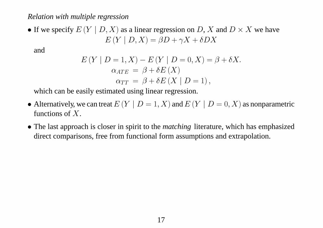
Relation with multiple regression

• If we specify E (Y | D,X) as a linear regression onD,X andD ×X we haveE (Y | D,X) = βD + γX + δDX

andE (Y | D = 1, X)−E (Y | D = 0, X) = β + δX.

αATE = β + δE (X)

αTT = β + δE (X | D = 1) ,which can be easily estimated using linear regression.

• Alternatively, we can treatE (Y | D = 1, X) andE (Y | D = 0, X) as nonparametricfunctions ofX .

• The last approach is closer in spirit to the matching literature, which has emphasizeddirect comparisons, free from functional form assumptions and extrapolation.

17

Imputing missing outcomes

• Suppose that X is discrete and takes on J values©ξjªJj=1

and we have a sample{Xi}Ni=1. LetNj = number of observations in cell j.Nj = number of observations in cell j withD = .Yj= mean outcome in cell j forD = .

• Thus,³Yj1 − Y j0

ís the sample counterpart of

E¡Y | D = 1, X = ξj

¢−E ¡Y | D = 0, X = ξj¢,

which can be used to get the estimates

bαATE = JXj=1

³Yj1 − Y j0

Ńj

N, bαTT = JX

j=1

³Yj1 − Y j0

Ńj1

N1

• The formula for bαTT can also be written in the formbαTT = 1

N1

XDi=1

³Yi − Y j(i)0

´where j (i) is the cell ofXi. Thus, bαTT matches the outcome of each treated unit withthe mean of the nontreated units in the same cell.

• IfX is continuous but low dimensional, the idea can be extended by matching obser-vations with similar or discretized values ofX .

18

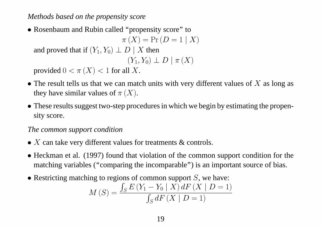
Methods based on the propensity score

• Rosenbaum and Rubin called ‘‘propensity score’’ toπ (X) = Pr (D = 1 | X)

and proved that if (Y1, Y0) ⊥ D | X then(Y1, Y0) ⊥ D | π (X)

provided 0 < π (X) < 1 for allX .

• The result tells us that we can match units with very different values of X as long asthey have similar values of π (X).

• These results suggest two-step procedures in which we begin by estimating the propen-sity score.

The common support condition

• X can take very different values for treatments & controls.

• Heckman et al. (1997) found that violation of the common support condition for thematching variables (‘‘comparing the incomparable’’) is an important source of bias.

• Restricting matching to regions of common support S, we have:

M (S) =

RS E (Y1 − Y0 | X) dF (X | D = 1)R

S dF (X | D = 1)

19

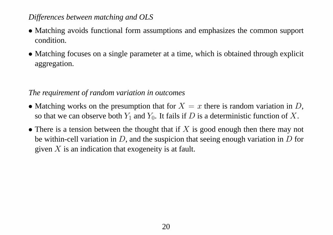
Differences between matching and OLS

• Matching avoids functional form assumptions and emphasizes the common supportcondition.

• Matching focuses on a single parameter at a time, which is obtained through explicitaggregation.

The requirement of random variation in outcomes

• Matching works on the presumption that for X = x there is random variation in D,so that we can observe both Y1 and Y0. It fails ifD is a deterministic function ofX .

• There is a tension between the thought that if X is good enough then there may notbe within-cell variation inD, and the suspicion that seeing enough variation inD forgivenX is an indication that exogeneity is at fault.

20

Example 2: Monetary incentives and schooling in the UK

• The pilot of the Education Maintenance Allowance (EMA) program started in Sept.1999. EMA paid youths aged 16–18 that continued in full time education (after 11compulsory grades) a weekly stipend of £ 30 to 40, plus final bonuses for good resultsup to £140.

• Eligibility (and amounts paid) depends on household characteristics. Eligible for fullpayments if annual income under £13000. Those above £30000, not eligible.

• Dearden, Emmerson, Frayne & Meghir (2002) participated in the design of the pilotand did the evaluation.

• No experimental design for political reasons, but one defining treatment and controlareas, both rural and urban.

• Basic question asked is whether more education results from this policy. The worry isthat families fail to decide optimally due to liquidity constraints or misinformation.

• They use propensity scores. Probit estimates of π (X) with family, local, and schoolcharacteristics. For each treated observation they construct a counterfactual mean us-ing kernel regression and bootstrap standard errors.

• EMA increased participation in year 12 by 5.9% for eligible individuals, and by 3.7%for the whole population. Only significant results for full-payment recipients.

21

V. Instrumental variables1. Instrumental variable assumptions

• Suppose we have non-experimental data with covariates, but cannot assume condi-tional independence as in matching:

(Y1, Y0) ⊥ D | X.• Suppose, however, that we have a variableZ that is an ‘‘exogenous source of variation

inD’’ in the sense that it satisfies the independence assumption :(Y1, Y0) ⊥ Z | X

and the relevance assumption :Z 0 D | X.

• Matching can be regarded as a special case of IV in which Z = D, i.e. all variation inD is exogenous givenX.

22

2. Instrumental-variable examples

Example 1: Non-compliance in randomized trials

• In a classic example, Z indicates assignment to treatment in an experimental design.Therefore, (Y1, Y0) ⊥ Z.

• However, ‘‘actual treatment’’D differs from Z because some individuals in the treat-ment group decide not to treat (non-compliers). Z andD will be correlated in general.

• Assignment to treatment is not a valid instrument in the presence of externalities thatbenefit members of the treatment group even if they are not treated themselves. Insuch case the exclusion restriction fails to hold.

• An example of this situation arises in a study of the effect of deworming on schoolparticipation in Kenya using school-level randomization (Miguel and Kremer, Econo-metrica, 2004).

23

Example 2: Ethnic enclaves and immigrant outcomes

• Interest in the effect of leaving in a highly concentrated ethnic area on labor success.In Sweden 11% of the population was born abroad. Of those, more than 40% live inan ethnic enclave (Edin, Fredriksson and Åslund, QJE, 2003).

• The causal effect is ambiguous. Residential segregation lowers the acquisition rate oflocal skills, preventing access to good jobs. But enclaves act as opportunity-increasingnetworks by disseminating information to new immigrants.

• Immigrants in ethnic enclaves have 5% lower earnings, after controlling for age, edu-cation, gender, family background, country of origin, and year of immigration.

• But this association may not be causal if the decision to live in an enclave depends onexpected opportunities.

• Swedish governments of 1985-1991assigned initial areas of residence to refugee im-migrants. Motivated by the belief that dispersing immigrants promotes integration.

• Let Z indicate initial assignment (8 years before measuring ethnic enclave indicatorD). Edin et al. assumed that Z is independent of potential earnings Y0 and Y1.

• IV estimates implied a 13% gain for low-skill immigrants associated with one std.deviation increase in ethnic concentration. For high-skill immigrants there was noeffect.

24

Example 3: Vietnam veterans and civilian earnings

• Did military service in Vietnam have a negative effect on earnings? (Angrist, 1990).

• Here we have:– Instrumental variable: draft lottery eligibility.– Treatment variable: Veteran status.– Outcome variable: Log earnings.– Data: N = 11637 white men born 1950–1953.– March Population Surveys of 1979 and 1981–1985.

• This lottery was conducted annually during 1970-1974. It assigned numbers (from 1to 365) to dates of birth in the cohorts being drafted. Men with lowest numbers werecalled to serve up to a ceiling determined every year by the Department of Defense.

• Abadie (2002) uses as instrument an indicator for lottery numbers lower than 100.

• The fact that draft eligibility affected the probability of enrollment along with its ran-dom nature makes this variable a good candidate to instrument ‘‘veteran status’’.

• There was a strong selection process in the military during the Vietnam period. Somevolunteered, while others avoided enrollment using student or job deferments.

• Presumably, enrollment was influenced by future potential earnings.

25

3. Identification of causal effects in IV settings

• The question is whether the availability of an instrumental variable identifies causaleffects. To answer it, I consider a binary Z, and abstract from conditioning.

Homogeneous effects

• If the causal effect is the same for every individualY1i − Y0i = α

the availability of an IV allows us to identify α. This is the traditional situation ineconometric models with endogenous explanatory variables.

• In the homogeneous caseYi = Y0i + (Y1i − Y0i)Di = Y0i + αDi.

• Also, taking into account that Y0i ⊥ ZiE (Yi | Zi = 1) = E (Y0i) + αE (Di | Zi = 1)E (Yi | Zi = 0) = E (Y0i) + αE (Di | Zi = 0) .

• Subtracting both equations we obtain

α =E (Yi | Zi = 1)−E (Yi | Zi = 0)E (Di | Zi = 1)−E (Di | Zi = 0)

which determines α as long asE (Di | Zi = 1) 6= E (Di | Zi = 0) .

• Get the effect ofD on Y through the effect of Z because Z only affects Y throughD.26

Heterogeneous effectsSummary

• In the heterogeneous case the availability of IVs is not sufficient to identify a causaleffect.

• An additional assumption that helps identification of causal effects is the following‘‘monotonicity’’ condition: Any person that was willing to treat if assigned to the con-trol group, would also be prepared to treat if assigned to the treatment group.

• The plausibility of this assumption depends on the context of application.

• Under monotonicity, the IV coefficient coincides with the average treatment effect forthose whose value of D would change when changing the value of Z (local averagetreatment effect or LATE).

27

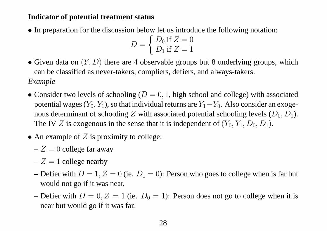
Indicator of potential treatment status

• In preparation for the discussion below let us introduce the following notation:

D =

½D0 if Z = 0D1 if Z = 1

• Given data on (Y,D) there are 4 observable groups but 8 underlying groups, whichcan be classified as never-takers, compliers, defiers, and always-takers.

Example

• Consider two levels of schooling (D = 0, 1, high school and college) with associatedpotential wages (Y0, Y1), so that individual returns areY1−Y0. Also consider an exoge-nous determinant of schooling Z with associated potential schooling levels (D0, D1).The IV Z is exogenous in the sense that it is independent of (Y0, Y1, D0, D1).

• An example of Z is proximity to college:– Z = 0 college far away– Z = 1 college nearby– Defier withD = 1, Z = 0 (ie. D1 = 0): Person who goes to college when is far but

would not go if it was near.– Defier with D = 0, Z = 1 (ie. D0 = 1): Person does not go to college when it is

near but would go if it was far.

28

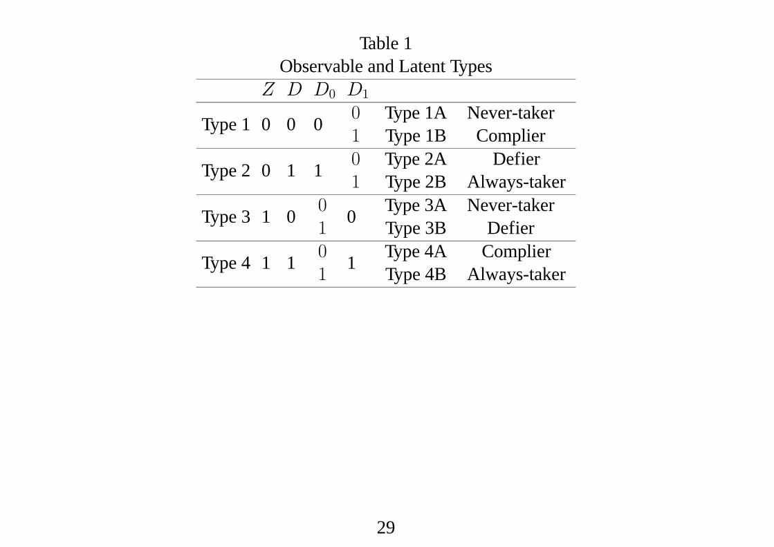
Table 1Observable and Latent Types

Z D D0 D1

Type 1 0 0 0 01

Type 1AType 1B

Never-takerComplier

Type 2 0 1 1 01

Type 2AType 2B

DefierAlways-taker

Type 3 1 0 01

0 Type 3AType 3B

Never-takerDefier

Type 4 1 1 01

1 Type 4AType 4B

ComplierAlways-taker

29

Availability of IV is not sufficient by itself to identify causal effects

• Note that sinceE (Y | Z = 1) = E (Y0) +E [(Y1 − Y0)D1]E (Y | Z = 0) = E (Y0) +E [(Y1 − Y0)D0]

we haveE (Y | Z = 1)−E (Y | Z = 0) = E [(Y1 − Y0) (D1 −D0)]= E (Y1 − Y0 | D1 −D0 = 1)Pr (D1 −D0 = 1)−E (Y1 − Y0 | D1 −D0 = −1) Pr (D1 −D0 = −1)

• E (Y | Z = 1)−E (Y | Z = 0) could be negative and yet the causal effect be positivefor everyone, as long as the probability of defiers is sufficiently large.

30

4. Local average treatment effects (LATE)Monotonicity and LATEs

• If we rule out defiers i.e. Pr (D1 −D0 = −1) = 0, we haveE (Y | Z = 1)−E (Y | Z = 0) = E (Y1 − Y0 | D1 −D0 = 1)Pr (D1 −D0 = 1)andE (D | Z = 1)−E (D | Z = 0) = E (D1)−E (D0) = Pr (D1 −D0 = 1) .

• Therefore,

E (Y1 − Y0 | D1 −D0 = 1) = E (Y | Z = 1)−E (Y | Z = 0)E (D | Z = 1)−E (D | Z = 0)

• Imbens and Angrist called this parameter ‘‘local average treatment effects’’ (LATE).

• Different IV’s lead to different parameters, even under instrument validity, which iscounter to standard GMM thinking.

• Policy relevance of a LATE parameter depends on the subpopulation of compliersdefined by the instrument. Most relevant LATE’s are those based on instruments thatare policy variables (eg college fee policies or college creation).

• What happens if there are no compliers? In the absence of defiers, the probability ofcompliers satisfies

Pr (D1 −D0 = 1) = E (D | Z = 1)−E (D | Z = 0) .So, lack of compliers implies lack of instrument relevance, hence underidentification.

32

Distributions of potential wages for compliers

• Imbens and Rubin (1997) showed that under monotonicity not only the average treat-ment effect for compliers is identified but also the entire marginal distributions of Y0and Y1 for compliers.

• Abadie (2002) gives a simple proof that suggests a Wald calculation. For any functionh (.) let us consider

W = h (Y )D =

½W1 = h (Y1) ifD = 1W0 = 0 ifD = 0 .

Because (W1,W0, D1, D0) are independent of Z, we can apply the LATE formula toW and get

E (W1 −W0 | D1 −D0 = 1) = E (W | Z = 1)−E (W | Z = 0)E (D | Z = 1)−E (D | Z = 0) ,

or substituting

E (h (Y1) | D1 −D0 = 1) = E (h (Y )D | Z = 1)−E (h (Y )D | Z = 0)E (D | Z = 1)−E (D | Z = 0) .

• If we choose h (Y ) = 1 (Y ≤ r), the previous formula gives as an expression for thecdf of Y1 for the compliers.

33

• Similarly, if we consider

V = h (Y ) (1−D) =½V1 = h (Y0) if 1−D = 1V0 = 0 if 1−D = 0

thenE (V1 − V0 | D1 −D0 = 1) = E (V | Z = 1)−E (V | Z = 0)

E (1−D | Z = 1)−E (1−D | Z = 0)or

E (h (Y0) | D1 −D0 = 1) = E (h (Y ) (1−D) | Z = 1)−E (h (Y ) (1−D) | Z = 0)E (1−D | Z = 1)−E (1−D | Z = 0)

from which we can get the cdf ofY0 for the compliers, again settingh (Y ) = 1 (Y ≤ r).• To see the intuition, suppose that D is exogenous (i.e. Z = D), then the cdf ofY | D = 0 coincides with the cdf of Y0, and the cdf of Y | D = 1 coincides with thecdf of Y1.

• If we regress h (Y )D onD, the OLS regression coefficient isE [h (Y )D | D = 1]−E [h (Y )D | D = 0] = E [h (Y1)]

which for h (Y ) = 1 (Y ≤ r) gives us the cdf of Y1.

• Similarly, if we regress h (Y ) (1−D) on (1−D), the regression coefficient isE [h (Y ) (1−D) | 1−D = 1]−E [h (Y ) (1−D) | 1−D = 0] = E [h (Y0)] .

• In the IV case, we are running similar IV (instead of OLS) regressions using Z asinstrument and getting expected h (Y1) and h (Y0) for compliers.

34

Conditional estimation with instrumental variables

• So far we abstracted from the fact that the validity of the instrument may only beconditional onX: It may be that (Y0, Y1) ⊥ Z does not hold, but the following does:

(Y0, Y1) ⊥ Z | X (conditional independence)Z 0 D | X (conditional relevance)

• For example, in the analysis of returns to college where Z is an indicator of proximityto college. The problem is that Z is not randomly assigned but chosen by parents, andthis choice may depend on characteristics that subsequently affect wages. The validityof Z may be more credible given family background variablesX .

• In a linear version of the problem:– First stage: RegressD on Z andX → get bD.– Second stage: Regress Y on bD andX .

• In general we now have conditional LATE givenX:γ (X) = E (Y1 − Y0 | D1 6= D0, X) .

• On the other hand, we have conditional IV estimands:

β (X) =E (Y | Z = 1, X)−E (Y | Z = 0, X)E (D | Z = 1, X)−E (D | Z = 0, X)

35

• What is the relevant aggregate effect? If the treatment effect is homogeneous givenXY1 − Y0 = β (X) ,

then a parameter of interest is:

E [β (X)] =

Zβ (X) dF (X) .

• However, in the case of heterogeneous effects, it makes sense to consider an averagetreatment effect for the overall subpopulation of compliers:

βC =

Zβ (X) dF (X | compliers) .

• Calculating βC appears problematic because F (X | compliers) is unobservable, but

βC =

Zβ (X)

Pr (compliers | X)Pr (compliers)

dF (X)

=

Z[E (Y | Z = 1, X)−E (Y | Z = 0, X)] 1

Pr (compliers)dF (X)

wherePr (compliers) =

Z[E (D | Z = 1, X)−E (D | Z = 0, X)] dF (X) .

• Therefore,

βC =

R[E (Y | Z = 1, X)−E (Y | Z = 0, X)] dF (X)R[E (D | Z = 1, X)−E (D | Z = 0, X)] dF (X),

which can be estimated as a ratio of matching estimators (Frölich, 2003).36

5. Relating LATE to parametric models of the potential outcomes5.1 The endogenous dummy explanatory variable probit model

• The model as usually written in terms of observables isY = 1 (α + βD + U ≥ 0)D = 1 (π0 + π1Z + V ≥ 0)µUV

¶| Z ∼ N

∙0,

µ1 ρρ 1

¶¸.

• In this modelD is an endogenous explanatory variable as long as ρ 6= 0. D is exoge-nous if ρ = 0.

• In this model there are only two potential outcomes:Y1 = 1 (α + β + U ≥ 0)Y0 = 1 (α + U ≥ 0)

• The average probability effect of interest (ATE) is given byθ = E (Y1 − Y0) = Φ (α + β)− Φ (α) .

• In less parametric specificationsE (Y1 − Y0)may not be point identified, but we maystill be able to estimate LATE.

37

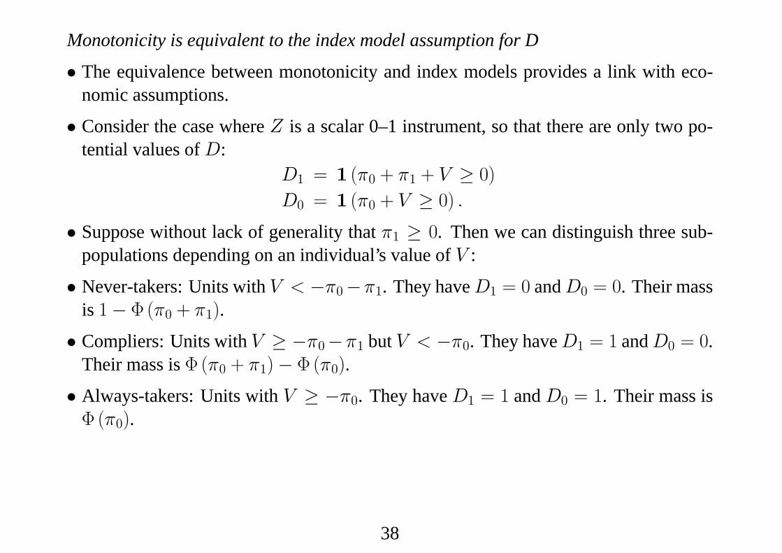
Monotonicity is equivalent to the index model assumption for D

• The equivalence between monotonicity and index models provides a link with eco-nomic assumptions.

• Consider the case where Z is a scalar 0–1 instrument, so that there are only two po-tential values ofD:

D1 = 1 (π0 + π1 + V ≥ 0)D0 = 1 (π0 + V ≥ 0) .

• Suppose without lack of generality that π1 ≥ 0. Then we can distinguish three sub-populations depending on an individual’s value of V :

• Never-takers: Units with V < −π0−π1. They haveD1 = 0 andD0 = 0. Their massis 1− Φ (π0 + π1).

• Compliers: Units with V ≥ −π0−π1 but V < −π0. They haveD1 = 1 andD0 = 0.Their mass is Φ (π0 + π1)− Φ (π0).

• Always-takers: Units with V ≥ −π0. They have D1 = 1 and D0 = 1. Their mass isΦ (π0).

38

LATE under joint probit assumptions

• Let us obtain the average treatment effect for the subpopulation of compliers:θLATE = E (Y1 − Y0 | D1 −D0 = 1) ≡ E (Y1 − Y0 | −π0 − π1 ≤ V < −π0) .

• We haveE (Y1 | −π0 − π1 ≤ V < −π0) = Pr (α + β + U ≥ 0 | −π0 − π1 ≤ V < −π0)= 1− Pr (U ≤ −α− β, V ≤ −π0)− Pr (U ≤ −α− β, V ≤ −π0 − π1)

Pr (V ≤ −π0)− Pr (V ≤ −π0 − π1)and similarlyE (Y0 | −π0 − π1 ≤ V < −π0) = Pr (α + U ≥ 0 | −π0 − π1 ≤ V < −π0)

= 1− Pr (U ≤ −α, V ≤ −π0)− Pr (U ≤ −α, V ≤ −π0 − π1)

Pr (V ≤ −π0)− Pr (V ≤ −π0 − π1).

• Finally,

θLATE =1

Φ (−π0)− Φ (−π0 − π1)[Φ2 (−α,−π0; ρ)− Φ2 (−α,−π0 − π1; ρ)

−Φ2 (−α− β,−π0; ρ) + Φ2 (−α− β,−π0 − π1; ρ)] .

where Φ2 (r, s; ρ) = Pr (U ≤ r, V ≤ s) is a standard normal bivariate probability.

• The nice thing about θLATE is that it is identified from the Wald formula in the absenceof joint normality.

• In fact, it does not even require monotonicity in the relationship between Y andD.

39

5.2 Models with additive errors: switching regressionsThe switching regression model with endogenous switch

• The model is as follows:Yi = α + βiDi + Ui

Di = 1 (γ0 + γ1Zi + εi ≥ 0) (1)

• The potential outcomes areY1i = α + βi + Ui ≡ μ1 + V1iY0i = α + Ui ≡ μ0 + V0i

so that the treatment effect βi = Y1i − Y0i is heterogeneous.

• Traditional models assume that βi is constant or that it varies only with observablecharacteristics. In these models D may be exogenous (independent of U ) or endoge-nous (correlated with U ) but in either case Y1− Y0 is constant, at least given controls.

• βi may depend on unobservables andDi may be correlated with both Ui and βi.

• We assume the exclusion restriction holds in the sense that (V1i, V0i, εi) or (Ui,βi, εi)are independent of Zi.

• In terms of the alternative notation (letting α = μ0 and Ui = V0i):Yi = μ0 + (Y1i − Y0i)Di + V0i = μ0 + (μ1 − μ0)Di + [V0i + (V1i − V0i)Di] .

• Let us write the ATE as β = μ1 − μ0 and ξi = V1i − V0i so that βi = β + ξi.

40

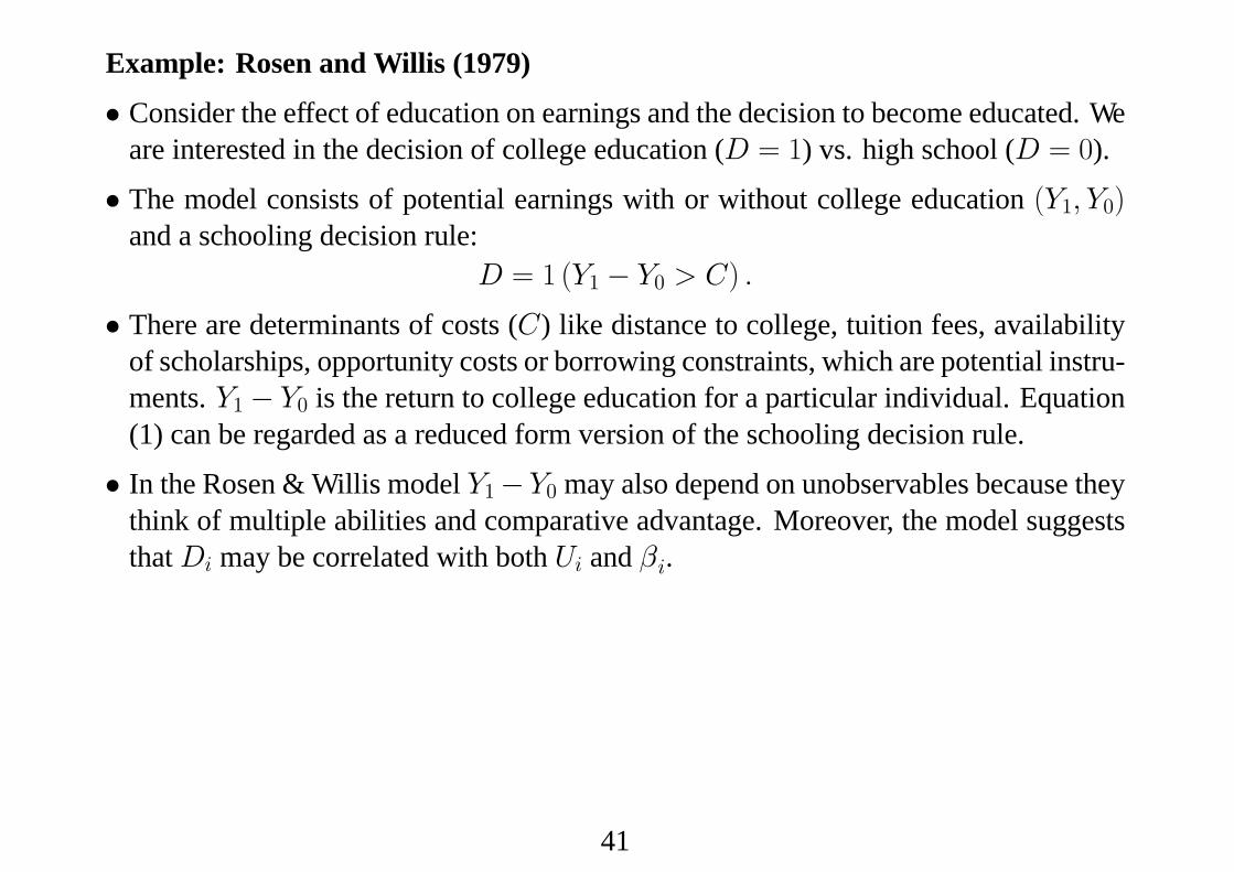
Example: Rosen and Willis (1979)

• Consider the effect of education on earnings and the decision to become educated. Weare interested in the decision of college education (D = 1) vs. high school (D = 0).

• The model consists of potential earnings with or without college education (Y1, Y0)and a schooling decision rule:

D = 1 (Y1 − Y0 > C) .• There are determinants of costs (C) like distance to college, tuition fees, availability

of scholarships, opportunity costs or borrowing constraints, which are potential instru-ments. Y1− Y0 is the return to college education for a particular individual. Equation(1) can be regarded as a reduced form version of the schooling decision rule.

• In the Rosen & Willis model Y1−Y0 may also depend on unobservables because theythink of multiple abilities and comparative advantage. Moreover, the model suggeststhatDi may be correlated with both Ui and βi.

41

Endogeneity and self-selection

• WriteE (Yi | Zi) = μ0 + (μ1 − μ0)E (Di | Zi) +E (V1i − V0i | Di = 1, Zi)E (Di | Zi) .• If βi is mean independent ofDi

E (Yi | Zi) = μ0 + (μ1 − μ0)E (Di | Zi) .so that β = Cov (Z, Y ) /Cov (Z,D).

• Otherwise, β does not coincide with the IV estimand. A special case of mean inde-pendence of βi with respect toDi occurs when βi is constant.

• The failure of IV can be seen as the result of a missing variable. The model can bewritten as

Yi = α + βDi + ϕ (Zi)Di + ζ iwhere ϕ (Zi) = E (V1i − V0i | Di = 1, Zi). Note that E (ζ i | Zi) = 0.

• When we do ordinary IV estimation we are not taking into account the variableϕ (Zi)Di.

• ϕ (z) is the average excess return for college-educated people with Zi = z. In thedistance to college example (Z = 1 if college near), we would expect ϕ (1) ≤ ϕ (0).

• The average treatment effect on the treated and the LATE are, respectively,αTT = E (Y1i − Y0i | Di = 1) = β +E (V1i − V0i | Di = 1) ,

αLATE = E (Y1i − Y0i | D1i −D0i = 1) = β+E (V1i − V0i | −γ0 − γ1 ≤ εi < −γ0) .42

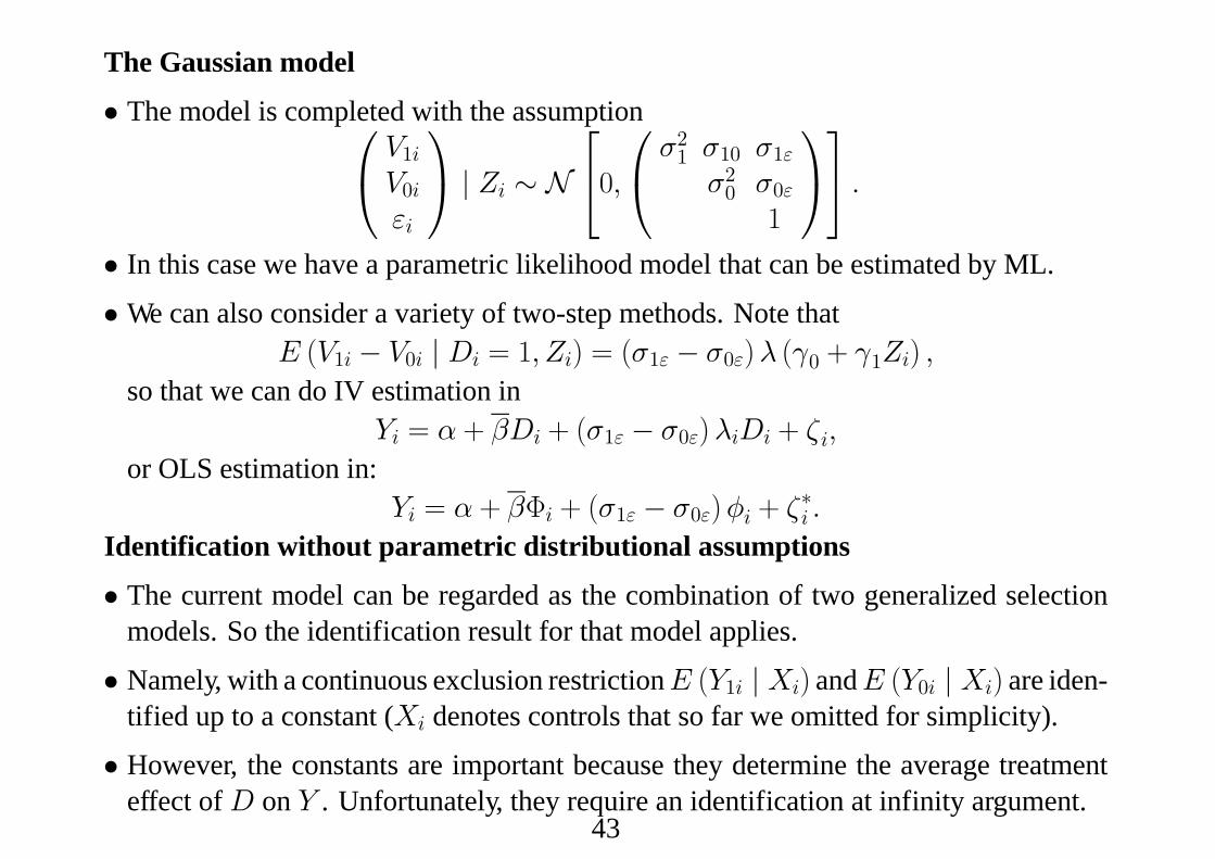
The Gaussian model

• The model is completed with the assumption⎛⎝ V1iV0iεi

⎞⎠ | Zi ∼ N⎡⎣0,

⎛⎝ σ21 σ10 σ1εσ20 σ0ε

1

⎞⎠⎤⎦ .• In this case we have a parametric likelihood model that can be estimated by ML.

• We can also consider a variety of two-step methods. Note thatE (V1i − V0i | Di = 1, Zi) = (σ1ε − σ0ε)λ (γ0 + γ1Zi) ,

so that we can do IV estimation inYi = α + βDi + (σ1ε − σ0ε)λiDi + ζ i,

or OLS estimation in:Yi = α + βΦi + (σ1ε − σ0ε)φi + ζ∗i .

Identification without parametric distributional assumptions

• The current model can be regarded as the combination of two generalized selectionmodels. So the identification result for that model applies.

• Namely, with a continuous exclusion restrictionE (Y1i | Xi) andE (Y0i | Xi) are iden-tified up to a constant (Xi denotes controls that so far we omitted for simplicity).

• However, the constants are important because they determine the average treatmenteffect ofD on Y . Unfortunately, they require an identification at infinity argument.

43

6. Marginal treatment effectsIntroduction

• When the support of Z is not binary, there is a multiplicity of causal effects.

• What causal effects are relevant for evaluating a given policy?

• The natural experiment literature has been satisfied with identifying ‘‘causal effects’’,without paying much attention to their relevance.

• If Z is continuous we can define a different LATE parameter for every pair (z, z0):

αLATE (z, z0) =

E (Y | Z = z)−E (Y | Z = z0)E (D | Z = z)−E (D | Z = z0).

The multiplicity is even higher when there is more than one instrument.IV assumptions and monotonicity

• For a general instrument vector Z, there are as many potential treatment status indica-torsDz as possible values z of the instrument. The IV assumptions become:– Independence: (Y1, Y0, Dz) ⊥ Z.– Relevance: Pr (D = 1 | Z = z) = P (z) is a nontrivial function of z.

• The monotonicity assumption for general Z can be expressed as follows. For any pairof values (z, z0) either

Dzi ≥ Dz0i or Dzi ≤ Dz0ifor all units in the population.

44

Latent index representation

• Alternatively we can postulate an index model forDz:Dz = 1 (μ (z)− U > 0) and U ⊥ Z,

which can be a useful way of organizing different LATEs (Heckman & Vytlacil, 2005).

• Note that the observedD isD = DZ.

• Monotonicity and index model assumptions are equivalent (Vytlacil, 2002).

• This result connects LATE thinking with econometric selection models.

• Without loss of generality we can setμ (z) = P (z) and takeU as uniformly distributedin the (0, 1) interval. To see this note that

1 (μ (z) > U) = 1 {FU [μ (z)] > FU (U)} = 1³P (z) > eU´

where eU is uniformly distributed.

• To connect with the earlier discussion, ifZ is a 0–1 scalar instrument there are only twovalues of the propensity score P (0) and P (1). Suppose that P (0) < P (1). Always-takers have U < P (0), compliers have a value of U between P (0) and P (1), andnever-takers have U > P (1). A similar argument can be made for any pair (z, z0) inthe case of a general Z.

• So under monotonicity we can always invoke and index equation and imagine eachmember of the population as having a particular value of the unobserved variable U .

45

Marginal Treatment Effect

• Using the propensity score P (Z) = Pr (D = 1 | Z) as instrument, LATE becomes

αLATE (P (z) , P (z0)) =

E (Y | P (Z) = P (z))−E (Y | P (Z) = P (z0))P (z)− P (z0) .

• IfZ is binary this is equivalent to what we had in the first place, but ifZ is continuous,taking limits as z → z0, we get a limiting form of LATE or MTE:

MTE (P (z)) =∂E (Y | P (Z) = P (z))

∂P (z).

• αLATE (P (z) , P (z0)) gives the ATE for individuals who would change schooling sta-tus from changing P (Z) from P (z0) to P (z):

αLATE (P (z) , P (z0)) = E [Y1 − Y0 | P (z0) < U < P (z)]

• Similarly MTE (P (z)) gives the ATE for individuals who would change schoolingstatus following a marginal change in P (z) or, in other words, who are indifferentbetween schooling choices at P (Z) = P (z).

• Using the error term in the index model, we can say thatMTE (P (z)) = E (Y1 − Y0 | U = P (z))

46

• IntegratingMTE (P (z)) over different ranges of U we can get other ATE measures.For example,

αLATE (P (z) , P (z0)) =

R P (z)P (z0)MTE (u) du

P (z)− P (z0)• Moreover,

αATE =

Z 1

0

MTE (u) du,

which makes it clear that to be able to identifyαATE we need identification ofMTE (u)over the entire (0, 1) range.

Policy-relevant treatment effects

• Constructing suitably integratedMTE (u) s it may be possible to identify policy rel-evant treatment effects.

• LATE gives the per capita effect of the policy in those induced to change by the policywhen the instrument is precisely an indicator of the policy change.

• For example, policies that change college fees or distance to school, under the assump-tion that the policy change affects the probability of participation but not the gain itself.

47

Estimation: Local IV method

• Heckman and Vytlacil suggest to estimate MTE by estimating the derivative of theconditional mean

E (Y | P (Z) = P (z) , X = x)using kernel-based local linear regression techniques.

• Note that in this context the propensity score plays a very different role to matching.

• Testing for homogeneity (or absence of self-selection) : A test of linearity on the propen-sity score (conditional onX) is a test of homogeneity of treatment effects.

• To see this use Y = Y0 + (Y1 − Y0)D and writeE (Y | P (Z)) = E (Y0 | P (Z)) +E ((Y1 − Y0)D | P (Z))

= E (Y0) +E [Y1 − Y0 | D = 1, P (Z)]P (Z)• The quantity E [Y1 − Y0 | D = 1, P (Z)] is constant under homogeneity, so that the

conditional mean E (Y | P (Z)) is linear in P (Z).

48

Remarks about unobserved heterogeneity in IV settings

• How important is it?– The balance between observed and unobserved heterogeneity depends on how de-

tailed information on agents is available (an empirical issue).– The worry for IV-based identification of treatment effects is not heterogeneity per

se, but the fact that heterogeneous gains may affect program participation.

• Warnings:– In the absence of an economic model or a clear notional experiment, it is often dif-

ficult to interpret what IV estimates estimate.– Knowing that IV estimates can be interpreted as averages of heterogeneous effects is

not very useful if understanding the heterogeneity itself is first order (Deaton, 2009).

• Heterogeneity of gains vs. heterogeneity of treatments– Heterogeneity of treatments may be more important. For example, the literature has

found significant differences in returns to different college majors.– A problem of aggregating educational categories is that returns are less meaningful.– Sometimes education outcomes are aggregated into just two categories because some

techniques are only well developed for binary explanatory variables.– A methodological emphasis may offer new opportunities but also impose constraints.

49

VI. Regression discontinuity methods1. Introduction and examples

• In the matching context we make the conditional exogeneity assumption(Y1, Y0) ⊥ D | X

whereas in the IV context we assume(Y1, Y0) ⊥ Z | X (independence)

D 0 Z | X (relevance).The relevance condition can also be expressed as saying that for some z 6= z0

Pr (D = 1 | Z = z) 6= Pr (D = 1 | Z = z0) .• In regression discontinuity we consider a situation where there is a continuous vari-

able Z that is not necessarily a valid instrument (it does not satisfy the exogeneityassumption), but such that treatment assignment is a discontinuous function of Z.

• The basic asymmetry on which identification rests is discontinuity in the dependenceofD on Z but continuity in the dependence of (Y1, Y0) on Z.

• RD methods have much potential in economic applications because geographic bound-aries or program rules often create usable discontinuities.

50

Examples

• Effect of class size on test scores (‘‘Maimonides’ rule’’ in Israel, Angrist & Lavy, 1999):Yis : average score at class i in school sDis : size of class i (not binary)Zs : beginning of year enrollment in school s

Maimonides’ rule allows enrollment cohorts of 1–40 to be grouped in a single class,but enrollment groups of 41–80 are split into two classes of average size 20.5–40,enrollment groups of 81–120 are split into three classes of average size 27–40, etc. Inpractice, the rule was not exact: class size predicted by the rule differed from actualsize.

51

Examples (continued)

• Effect of financial aid offers on students’ enrollment decisions (van der Klaauw, 2002)Yi : decision of student i to enroll in college ‘‘X’’ (binary)Di : amount of financial aid offer to student iZi : index that aggregates SAT score and high school GPA

Applicants for aid were divided into four groups on the basis of the interval the indexZ fell into. Average aid offers as a function of Z contained jumps at the cutoff pointsfor the different ranks, with those scoring just below a cutoff point receiving much lesson average than those who scored just above the cutoff.

• Do parties matter for economic outcomes? (Petterson-Lidbom, 2006; Arellano & Ben-tolila, in progress):

Yi : economic outcome in area iDi : party control indicator in local government iZi : vote share

52

2. The fundamental RD assumption

• We can now state the basic RD assumption more formally. Namely, discontinuity intreatment assignment but continuity in potential outcomes: There is at least a knownvalue z = z0 such that

limz→z+0

Pr (D = 1 | Z = z) 6= limz→z−0

Pr (D = 1 | Z = z) (2)

limz→z+0

Pr (Yj ≤ r | Z = z) = limz→z−0

Pr (Yj ≤ r | Z = z) (j = 0, 1) (3)

Implicit regularity conditions are: (i) the existence of the limits, and (ii) that Z haspositive density in a neighborhood of z0.

• We abstract from conditioning covariates for the time being for simplicity.

Sharp and fuzzy designs

• The early RD literature in psychology (Cook & Campbell 1979) distinguished between‘‘sharp’’ and ‘‘fuzzy’’ designs. In the former,D is a deterministic function of Z:

D = 1 (Z ≥ z0)whereas in the latter is not.

• The sharp design can be regarded as a special case of the fuzzy design, but one thathas different implications for identification of treatment effects. In the sharp design

limz→z+0

E (D | Z = z) = 1, limz→z−0

E (D | Z = z) = 0.

53

3. Homogeneous treatment effects

• Like in the IV setting, the case of homogeneous treatment effects is useful to presentthe basic RD estimand. Suppose that α = Y1 − Y0 is constant, so that

Yi = αDi + Y0i

• Taking conditional expectations given Z = z and left- and right-side limits:limz→z+0

E (Y | Z = z) = α limz→z+0

E (D | Z = z) + limz→z+0

E (Y0 | Z = z)limz→z−0

E (Y | Z = z) = α limz→z−0

E (D | Z = z) + limz→z−0

E (Y0 | Z = z) .• The RD assumption then leads to consideration of the following RD parameter

γ =limz→z+0 E (Y | Z = z)− limz→z−0 E (Y | Z = z)limz→z+0 E (D | Z = z)− limz→z−0 E (D | Z = z)

which is determined provided the ‘‘relevance part’’ (2) of the RD assumption is satis-fied, and equals α provided the ‘‘independence part’’ (3) of the RD assumption holds.

54

• In the case of a sharp design, the denominator is unity so thatγ = lim

z→z+0E (Y | Z = z)− lim

z→z−0E (Y | Z = z) , (4)

which can be regarded as a matching-type situation, in the same way that the generalcase can be regarded as an IV-type situation.

• So the basic idea is to obtain a treatment effect by comparing the average outcome leftof the discontinuity with the average outcome to the right of discontinuity, relative tothe difference between the left and right propensity scores.

• Intuitively, considering units within a small interval around the cutoff point is similarto a randomized experiment at the cutoff point.

55

4. Heterogeneous treatment effects

• Now suppose thatYi = αiDi + Y0i

• In the sharp design sinceDi = 1 (Z ≥ z0) we haveE (Y | Z = z) = E (α | Z = z) 1 (z ≥ z0) +E (Y0 | Z = z) .

• Therefore, the situation is one of selection on observables. That is, lettingk (z) = E (Y0 | Z = z) + [E (α | Z = z)−E (α | Z = z0)] 1 (z ≥ z0)

we haveE (Y | Z = z) = E (α | Z = z0) 1 (z ≥ z0) + k (z)

where k (z) is continuous at z = z0.

• Therefore, the OLS population coefficient onD in the equationY = γD + k (z) + w (5)

coincides with γ, which in turn equals E (α | Z = z0).• The control function k (z) is nonparametrically identified. To see this, first note thatγ is identified from (4). Then k (z) is identifiable as the nonparametric regressionE (Y − γD | Z = z). Note that if the treatment effect is homogeneousk (z) coincideswith E (Y0 | Z = z), but not in general.

56

• If μ (z) ≡ E (Y0 | Z = z) was known (e.g. using data from a setting in which noprogram was present) then we could consider a regression of Y on D and μ (z). Itturns out that the coefficient onD in such a regression is E (α | z ≥ z0).

• In the fuzzy design, D not only depends on 1 (Z ≥ z0) but also on other unobservedvariables. Thus, D is an endogenous variable in equation (5). However, we can stilluse 1 (Z ≥ z0) as an instrument for D in such equation to identify γ, at least in thehomogeneous case.

• The connection between the fuzzy design and the instrumental variables perspectivewas first made explicit in van der Klaauw (2002).

• Next, we discuss the interpretation of γ in the fuzzy design with heterogeneous treat-ment effects, under two different assumptions.

57

Monotonicity near z0• Hahn, Todd, and van der Klaauw (2001) also consider an alternative LATE-type of

assumption. Let Dz be the potential assignment indicator associated with Z = z,and for some ε > 0 and any pair (z0 − ε, z0 + ε) with 0 < ε < ε suppose the localmonotonicity assumption

Dz0+ε ≥ Dz0−ε for all units in the population.

• An example is a population of cities where Z denotes voting share and Dz is an in-dicator of party control when Z = z. In this case the local conditional independenceassumption could be problematic but the monotonicity assumption is not.

• In such case, it can be shown that γ identifies the local average treatment effect atz = z0:

γ = limε→0+

E (Y1 − Y0 | Dz0+ε −Dz0−ε = 1)i.e. the ATE for the units for whom treatment changes discontinuously at z0.

• If the policy is a small change in the threshold for program entry, the LATE parameterdelivers the treatment effect for the subpopulation affected by the change, so that inthat case it would be the parameter of policy interest.

60

5. Estimation strategies

• There are parametric and semiparametric strategies.A nonparametric Wald estimator

• Hahn-Todd-van der Klaauw suggested the following local Wald estimator. Let Si ≡1 (z0 − h < Zi < z0 + h) where h > 0 denotes the bandwidth, and consider the sub-sample such that Si = 1.

• The proposed estimator is the IV regression ofYi onDi usingWi ≡ 1 (z0 < Zi < z0 + h)as an instrument, applied to the subsample with Si = 1:bγ = bE (Yi |Wi = 1, Si = 1)− bE (Yi |Wi = 0, Si = 1)bE (Di |Wi = 1, Si = 1)− bE (Di |Wi = 0, Si = 1)

.

• This estimator has nevertheless a poor boundary performance. An alternative sug-gested by HTV is a local linear regression method.

61

Parametric and semiparametric alternatives

• SupposeE (D | Z) = g (Z) + δ1 (Z ≥ z0)

andE (Y0 | Z) = k (Z) .

• A control function regression-based approach is based in the control function aug-mented equation that replacesD by the propensity score E (D | Z):

Y = γE (D | Z) + k (Z) + w• In a parametric approach, we assume functional forms for g (Z) and k (Z). van der

Klaauw (2002) considered a semiparametric approach using a power series approxi-mation for k (Z).

• If g (Z) = k (Z), then we can do 2SLS using as instrumental variables{1 (Z ≥ z0) , g (Z)} ,

where g (Z) is the ‘‘included’’ instrument and 1 (Z ≥ z0) is the ‘‘excluded’’ instrument.

• These methods of estimation, which are not local to data points near the threshold, areimplicitly predicated on the assumption of homogeneous treatment effects.

62

6. Distributional effects

• For some function h (.), consider the outcome

W = h (Y )D =

½W1 = h (Y1) ifD = 1W0 = 0 ifD = 0

• Using h (Y ) = 1 (Y ≤ r), the RD parameter for the outcome W (r) = 1 (Y ≤ r)Ddelivers

Pr (Y1 ≤ r | Z = z0) =limz→z+0 E (W (r) | Z = z)− limz→z−0 E (W (r) | Z = z)

limz→z+0 E (D | Z = z)− limz→z−0 E (D | Z = z)under the local conditional independence assumption.

• A similar strategy can be followed to obtain Pr (Y0 ≤ r | Z = z0). In that case weconsider

V = h (Y ) (1−D) =½V1 = h (Y0) if 1−D = 1V0 = 0 if 1−D = 0 .

• The RD parameter for the outcome V (r) = 1 (Y ≤ r) (1−D) delivers

Pr (Y0 ≤ r | Z = z0) =limz→z+0 E (V (r) | Z = z)− limz→z−0 E (V (r) | Z = z)limz→z+0 E (D | Z = z)− limz→z−0 E (D | Z = z)

.

63

7. Conditioning on covariates

• Even if the RD assumption is satisfied unconditionally, conditioning on covariates maymitigate the heterogeneity in treatment effects, hence contributing to the relevance ofRD estimated parameters.

• Covariates may also make the local conditional exogeneity assumption more credible.

• This would also be true of within-group estimation in a panel data context (see Hoxby,QJE, 2000, 1239–1285, for an application).

64

VII. Differences in differencesExample: minimum wages and employment

• In March 1992 the state of New Jersey increased the legal minimum wage by 19%,whereas the bordering state of Pennsylvania kept it constant.

• Card and Krueger (1994) evaluated the effect of this change on the employment of lowwage workers. In a competitive model the result of increasing the minimum wage isto reduce employment.

• They conducted a survey to some 400 fast food restaurants from the two states justbefore the NJ reform, and a second survey to the same outlets 7-8 months after.

• Characteristics of fast food restaurants:(a) A large source of employment for low-wage workers.(b) They comply with minimum wage regulations (especially franchised restaurants).(c) Fairly homogeneous job, so good measures of employment and wages can be

obtained.(d) Easy to get a sample frame of franchised restaurants (yellow pages) with high

response rates.(e) Response rates 87% and 73% (less in Penn, because the interviewer was less

persistent).

65

• The DID coefficient isβ = [E (Y2 | D = 1)−E (Y1 | D = 1)]

− [E (Y2 | D = 0)−E (Y1 | D = 0)] .where Y1 and Y2 denote employment before and after the reform, D = 1 denotes astore in NJ (treatment group) andD = 0 in Penn (control group).

• β measures the difference between the average employment change in NJ and theaverage employment change in Penn.

• The key assumption in giving a causal interpretation to β is that the temporal effect inthe two states is the same in the absence of intervention.

• But it is possible to generalize the comparison in several ways, for example controllingfor other variables.

• Card and Krueger found that rising the minimum wage increased employment in someof their comparisons but in no case caused an employment reduction.

• This article originated much economic and political debate.

• DID estimation has become a very popular method of obtaining causal effects, espe-cially in the US, where the federal structure provides cross state variation in legislation.

66

The context of difference in difference comparisons

• If we observe outcomes before and after treatment, we could use the treated beforetreatment as controls for the treated after treatment.

• The problem of this comparison is that it can be contaminated by the effect of eventsother than the treatment that occurred between the two periods.

• Suppose that only a fraction of the population is exposed to treatment. In such a case,we can use the group that never receives treatment to identify the temporal variationin outcomes that is not due to exposure to treatment. This is the basic idea of the DIDmethod.

• Two-period potential outcomes with treatment in t = 2:Y1 = Y0 (1)

Y2 = (1−D)Y0 (2) +DY1 (2)• The fundamental identifying assumption is that the average changes in the two groups

are the same in the absence of treatment:E (Y0 (2)− Y0 (1) | D = 1) = E (Y0 (2)− Y0 (1) | D = 0) .

• Y0 (1) is always observed but Y0 (2) is counterfactual for units withD = 1.

• Under such identification assumption, the DID coefficient coincides with the averagetreatment effect for the treated.

67

• To see this note that the DID parameter in general is equal to:β = [E (Y2 | D = 1)−E (Y1 | D = 1)]− [E (Y2 | D = 0)−E (Y1 | D = 0)]

= E (Y1 (2) | D = 1)−E (Y0 (1) | D = 1)−[E (Y0 (2) | D = 0)−E (Y0 (1) | D = 0)]• Now, adding and subtracting E (Y0 (2) | D = 1):

β = E [Y1 (2)− Y0 (2) | D = 1]+ {E [Y0 (2)− Y0 (1) | D = 1]−E [Y0 (2)− Y0 (1) | D = 0]} ,

which as long as the last term vanishes it equalsβ = E [Y1 (2)− Y0 (2) | D = 1] .

68

Comments and problems

• β can be obtained as the coefficient of the interaction term in a regression of outcomeson treatment and time dummies.

• To obtain the DID parameter we do not need panel data (except if e.g. we regard theCard–Krueger data as an aggregate panel with two units and two periods), just cross-sectional data for at least two periods.

• With panel data, we can estimate β from a regression of outcome changes on the treat-ment dummy. This is convenient for accounting for dependence between the two pe-riods.

• Differences in the composition of the cross-sectional populations over time (especiallyproblematic if not using panel data).

• The fundamental assumption might be satisfied conditionally given certain covariates,but identification vanishes if some of them are unobservable.

69

VIII. Concluding remarksEmpirical work and empirical content

• Empirical papers have become more central to economics than they used to. Thisreflects the new possibilities afforded by technical change in research and is a sign ofscientific maturity of economics.

• In an empirical paper the econometric strategy is often paramount, i.e. what aspects ofdata to look at and how to interpret them. This typically requires a good understandingof both relevant theory and sources of variation in data. Once this is done there isusually a more or less obvious estimation method available and ways of assessingstatistical error.

• Statistical issues like quality of large sample approximations or measurement errormay or may not matter much in a particular problem, but a characteristic of a goodempirical paper is the ability to focus on the econometric problems that matter for thequestion at hand.

• The quasi-experimental approach is also having a contribution to reshaping structuraleconometric practice.

• It is increasingly becoming standard fare a reporting style that distinguishes clearly theroles of theory and data in getting the results.

70

Quasi-experimental approaches in policy evaluation

• Experimental and quasi-experimental approaches have an important but limited roleto play in policy evaluation.

• There are relevant quantitative policy questions that cannot be answered without thehelp of economic theory.

• In applied microeconomics there has been a lot of excitement in recent years in empir-ically establishing causal impacts of interventions (from field and natural experimentsand the like). This is understandable because in principle causal impacts are moreuseful for policy than correlations.

• However, there is an increasing awareness of the limitations due to heterogeneity ofresponses and interactions and dynamic feedback. Addressing these matters requiremore theory. A good thing of the treatment effect literature is that it has substantiallyraised the empirical credibility hurdle.

• A challenge for the coming years is to have more theory-based or structural empiricalmodels that are structural not just because the author has written down the model asderived from an utility function but because he/she has been able to establish empiri-cally invariance to a particular class of interventions, which therefore lends credibilityto the model for ex ante policy evaluation within this class.

71

econometric methods of program evaluation manuel …arellano/ief-evaluation-marellano-tr.pdf ·...

Documents