matching as an econometric evaluation estimator
TRANSCRIPT

Review of Economic Studies (1998) 65, 261-294 ^ 0034-6527/98/00120261$02.00
© 1998 The Review of Economic Studies Limited
Matching As An EconometricEvaluation Estimator
JAMES J. HECKMANUniversity of Chicago
HIDEHIKO ICHIMURA
University of Pittsburgh
and
PETRA TODDUniversity of Pennsylvania
First version received October 1994, final version accepted October 1997 (Eds.)
This paper develops the method of matching as an econometric evaluation estimator. Arigorous distribution theory for kernel-based matching is presented. The method of matching isextended to more general conditions than the ones assumed in the statistical literature on the topic.We focus on the method of propensity score matching and show that it is not necessarily better,in the sense of reducing the variance of the resulting estimator, to use the propensity score methodeven if propensity score is known. We extend the statistical literature on the propensity score byconsidering the case when it is estimated both parametrically and nonparametrically. We examinethe benefits of separability and exclusion restrictions in improving the efficiency of the estimator.Our methods also apply to the econometric selection bias estimator.
1. INTRODUCTION
Matching is a widely-used method of evaluation. It is based on the intuitively attractive ideaof contrasting the outcomes of programme participants (denoted Yi) with the outcomes of"comparable" nonparticipants (denoted yo). Differences in the outcomes between the twogroups are attributed to the programme.
Let /o and /i denote the set of indices for nonparticipants and participants, respec-tively. The following framework describes conventional matching methods as well as thesmoothed versions of these methods analysed in this paper. To estimate a treatment effectfor each treated person ie/i, outcome F,, is compared to an average of the outcomes Yojfor matched persons jelo in the untreated sample. Matches are constructed on the basisof observed characteristics X in R"". Typically, when the observed characteristics of anuntreated person are closer to those of the treated person ieli, using a specific distancemeasure, the untreated person gets a higher weight in constructing the match. The estima-ted gain for each person i in the treated sample is
(1)
where lVNo,N,(i,j) is usually a positive valued weight function, defined so that for each' ^ ^ 1 ' Z/e/ ^No.NXiJ) = ' and No and A i are the number of individuals in /o and / i ,respectively. The choice of a weighting function reflects the choice of a particular distancemeasure used in the matching method, and the weights are based on distances in the X
261
262 REVIEW OF ECONOMIC STUDIES
space. For example, for each ieli the nearest-neighhour method selects one individualjelo as the match whose Xj is the "closest" value to Z,, in some metric. The kernel methodsdeveloped in this paper construct matches using all individuals in the comparison sampleand downweighting "distant" observations.
The widely-used evaluation parameter on which we focus in this paper is the meaneffect of treatment on the treated for persons with characteristics X.
where Z)= 1 denotes programme participation. Heckman (1997) and Heckman and Smith(1998) discuss conditions under which this parameter answers economically interestingquestions. For a particular domain ^ for X, this parameter is estimated by
Lei, ^^o-NMiYu-Y^j^,^ W^o.NXi,J)Yoj], (2)
where different values of Wffo.NXi) may be used to select different domains ^ or to accountfor heteroskedasticity in the treated sample. Different matching methods are based ondifferent weighting functions {w^„,,^Xi)} and {fVi^.^NXiJ}}•
The method of matching is intuitively appealing and is often used hy applied statistici-ans, but not by economists. This is so for four reasons. First, it is difficult to determineif a particular comparison group is truly comparable to participants (i.e. would haveexperienced the same outcomes as participants had they participated in the programme).An ideal social experiment creates a valid comparison group. But matching on themeasured characteristics available in a typical nonexperimental study is not guaranteedto produce such a comparison group. The published literature presents conditional inde-pendence assumptions under which the matched group is comparable, but these are farstronger than the mean-independence conditions typically invoked by economists. More-over, the assumptions are inconsistent with many economic models of programme partici-pation in which agents select into the programme on the basis of unmeasured componentsof outcomes unobserved by the econometrician. Even if conditional independence isachieved for one set of X variables, it is not guaranteed to be achieved for other sets ofX variables including those that include the original variables as subsets. Second, if a validcomparison group can be found, the distribution theory for the matching estimator remainsto be established for continuously distributed match variables Z.'
Third, most of the current econometric literature is based on separability betweenobservables and unobservables and on exclusion restrictions that isolate different variablesthat determine outcomes and programme participation. Separability permits the definitionof parameters that do not depend on unobservables. Exclusion restrictions arise naturallyin economic models, especially in dynamic models where the date of enrollment into theprogramme differs from the dates when consequences of the programme are measured.The available literature on matching in statistics does not present a framework thatincorporates either type of a priori restriction.
Fourth, matching is a data-hungry method. With a large number of conditioningvariables, it is easy to have many cells without matches. This makes the method impracticalor dependent on the use of arbitrary sorting schemes to select hierarchies of matchingvariables. (See, e.g. Westat (1980,1982,1984).) In an important paper, Rosenbaum andRubin (1983) partially solve this problem. They establish that if matching on X is valid,so is matching solely on the probability of selection into the prograrrune PT(D=\\X)-
1. When the match variables are discrete, the matching estimator for each cell is a mean and consistencyand asymptotic normality of the matching estimator are easily established.
HECKMAN ET AL. MATCHING AS AN ESTIMATOR 263
P{X). Thus a multidimensional matching problem can be recast as a one-dimensionalproblem and a practical solution to the curse of dimensionality for matching is possible.^
Several limitations hamper the practical application of their theoretical result. Theirtheorem assumes that the probability of selection is known and is not estimated. It is alsobased on strong conditional independence assumptions that are difficult to verify in anyapplication and are unconventional in econometrics. They produce no distribution theoryfor their estimator.
In this paper we first develop an econometric framework for matching that allows usto incorporate additive separability and exclusion restrictions. We then provide a samplingtheory for matching from a nonparametric vantage point. Our distribution theory isderived under weaker conditions than the ones currently maintained in the statisticalliterature on matching. We show that the fundamental identification condition of thematching method for estimating (P-1) is
whenever both sides of this expression are well defined. In order for both sides to be welldefined simultaneously for all X it is usually assumed that O<P(X)<1 so thatSupp iX\D= 1) = Supp {X\D = G). As Heckman, Ichimura, Smith, Todd (1998), Heckman,Ichimura, Smith and Todd (19966) and Heckman, Ichimura and Todd (1997) point out,this condition is not appropriate for important applications of the method. In order tomeaningfully implement matching it is necessary to condition on the support common toboth participant and comparison groups S, where
S=Supp {X\D= 1) n Supp
and to estimate the region of common support. Equality of the supports need not holda priori although most formal discussions of matching assumes that it does. Heckman,Ichimura, Smith and Todd (1998) and Heckman, Ichimura and Todd (1997) report theempirical relevance of this point for evaluating job training programmes. Invokingassumptions that justify the application of nonparametric kernel regression methods toestimate programme outcome equations, maintaining weaker mean independenceassumptions compared to the conditional independence assumptions used in the literature,and conditioning on S, we produce an asymptotic distribution theory for matching estima-tors when regressors are either continuous, discrete or both. This theory is general enoughto make the Rosenbaum-Rubin theorem operational in the commonly-encountered casewhere P^X) is estimated either parametrically or nonparametrically.
With a rigorous distribution theory in hand, we address a variety of important ques-tions that arise in applying the method of matching: (1) We ask, if one knew the propensityscore, P{X), would one want to use it instead of matching on XI (2) What are the effectson asymptotic bias and variance if we use an estimated value of P? We address thisquestion both for the case of parametric and nonparametric PiX). Finally, we ask (3)what are the benefits, if any, of econometric separability and exclusion restrictions on thebias and variance of matching estimators?
The structure of this paper is as follows. Section 2 states the evaluation problem andthe parameters identified by the analysis of this paper. Section 3 discusses how matchingsolves the evaluation problem. We discuss the propensity score methodology of Rosen-baum and Rubin (1983). We emphasize the importance ofthe common support condition
2. They term P(X) the propensity score. For the relationship between propensity score methods andselection models, see Heckman and Robb (1986) or Heckman, Ichimura, Smith and Todd (1998).

264 REVIEW OF ECONOMIC STUDIES
assumed in the literature and develop an approach that does not require it. Section 4contrasts the assumptions used in matching with the separability assumptions and exclu-sion restrictions conventionally used in econometrics. A major goal of this paper is tounify the matching literature with the econometrics literature. Section 5 investigates acentral issue in the use of propensity scores. Even if the propensity score is known, is itbetter, in terms of reducing the variance of the resulting matching estimator, to conditionon X or P(X)? There is no unambiguous answer to this question. Section 6 presents abasic theorem that provides the distribution theory for kernel matching estimators basedon estimated propensity scores. In Section 7, these results are then applied to investigatethe three stated questions. Section 8 summarizes the paper.
2. THE EVALUATION PROBLEM AND THE PARAMETERS OF INTEREST
Each person can be in one of two possible states, 0 and 1, with associated outcomes(Jo, Yt), corresponding to receiving no treatment or treatment respectively. For example,"treatment" may represent participation in the social programme, such as the job trainingprogramme evaluated in our companion paper where we apply the methods developed inthis paper. (Heckman, Ichimura and Todd (1997).) Let D= 1 if a person is treated; £> =0 otherwise. The gain from treatment is A= 7 , - yo. We do not know A for anyonebecause we observe only Y=DYi + {l-D)Yo, i.e. either yo or y,.
This fundamental missing data problem cannot be solved at the level of any individual.Therefore, the evaluation problem is typically reformulated at the population level. Focus-ing on mean impacts for persons with characteristics X, a commonly-used parameter ofinterest for evaluating the mean impact of participation in social programmes is (P-1).It is the average gross gain from participation in the programme for participants withcharacteristics X. If the full social cost per participant is subtracted from (P-1) and theno treatment outcome for all persons closely approximates the no programme outcome,then the net gain informs us of whether the programme raises total social output comparedto the no programme state for the participants with characteristics X.^
The mean E(Yt\D=l,X) can be identified from data on programme participants.Assumptions must be invoked to identify the counterfactual mean E(Yo\D=l,X), theno-treatment outcome of programme participants. In the absence of data from an idealsocial experiment, the outcome of self-selected nonparticipants E(Yo\D = O,X) is oftenused to approximate E(Yo\D=l,X). The selection bias that arises from making thisapproximation is
Matching on X, or regression adjustment of yo using X, is based on the assumption thatB(X) = O so conditioning on X eliminates the bias.
Economists have exploited the idea of conditioning on observables using parametric ornonparametric regression analysis (Barnow, Cain and Goldberger (1980), Barros (1986),Heckman and Robb (1985, 1986)). Statisticians more often use matching methods, pairingtreated persons with untreated persons of the same X characteristics (Cochrane and Rubin(1973)).
The literature on programme evaluation gives two distinct responses to the problemof estimating (P-1) with continuous conditioning variables. The first borrows from the
3. See Heckman (1997) or Heckman and Smith (1998) for a precise statement of when this parameteranswers an mteresting economic evaluation question.

HECKMAN ET AL. MATCHING AS AN ESTIMATOR 265
kernel regression literature. It uses a smoothing procedure that borrows strength fromadjacent values of a particular value of A'=x and produces uniformly consistent estimatorsof (P-1) at all points of the support for the distributions oi X given D=\ or D = 0. (SeeHeckman, Ichimura, Smith and Todd (1996a) or Heckman, Ichimura and Todd (1997).)Parametric assumptions about E(Yo\D=l,X) play the same role as smoothingassumptions, and in addition allow analysts to extrapolate out of the sample for X. Unlessthe class of functions to which (P-1) may belong is restricted to be smaller than the finite-order continuously-diiferentiable class of functions, the convergence rate of an estimatorof (P-1) is governed by the number of continuous variables included in X (Stone (1982)).
The second response to the problem of constructing counterfactuals abandons estima-tion of (P-1) at any point of A' and instead estimates an average of (P-1) over an intervalof X values. Commonly-used intervals include Supp (X| i )=l) , or subintervals of thesupport corresponding to different groups of interest. The advantage of this approach isthat the averaged parameter can be estimated with rate A' "''' , where N is sample size,regardless of the number of continuous variables in X when the underlying functions aresmooth enough. Averaging the estimators over intervals ofX produces a consistent estima-tor of
M(5) = E(y,-yo | i )=l ,A'e5 ' ) , (P-2)
with a well-defined iV~' ^ distribution theory where S is a subset of Supp {X\D=l). Thereis considerable interest in estimating impacts for groups so (P-2) is the parameter ofinterest in conducting an evaluation. In practice both pointwise and setwise parametersmay be of interest. Historically, economists have focused on estimating (P-1) and statistici-ans have focused on estimating (P-2), usually defined over broad intervals of X values,including Supp (Jir|jD= 1). In this paper, we invoke conditions sufficiently strong to consist-ently estimate both (P-1) and (P-2).
3. HOW MATCHING SOLVES THE EVALUATION PROBLEM
Using the notation of Dawid (1979) let
denote the statistical independence of (yo, Yi) and D conditional on X. An equivalentformulation of this condition is
This is a non-causality condition that excludes the dependence between potentialoutcomes and participation that is central to econometric models of self selection. (SeeHeckman and Honore (1990).) Rosenbaum and Rubin (1983), henceforth denoted RR,establish that, when (A-1) and
0<P{X)<\, (A-2)
are satisfied, (yo, Yi)]LD\P{X), where P(X) = PT (£>= 1 IA'). Conditioning on PiX) bal-ances the distribution of yo and Yi with respect to D. The requirement (A-2) guaranteesthat matches can be made for all values of AT. RR called condition (A-1) an "ignorability"condition for D, and they call (A-1) and (A-2) together a "strong ignorability" condition.
When the strong ignorability condition holds, one can generate marginal distributionsof the counterfactuals
Foiyo\D=l,X) and F,(y,|£> = O,Ar),
266 REVIEW OF ECONOMIC STUDIES
but one cannot estimate the joint distribution of (yo, Yi), Fiyo,yi \D, X), without makingfurther assumptions about the structure of outcome and programme participationequations.'*
If PiX) = 0 or i'(A') = 1 for some values of Af, then one cannot use matching condi-tional on those X values to estimate a treatment effect. Persons with such X characteristicseither always receive treatment or never receive treatment, so matches from both D = 1and D = 0 distributions cannot be performed. Ironically, missing data give rise to theproblem of causal inference, but missing data, i.e. the unobservables producing variationin D conditional on X, are also required to solve the problem of causal inference. Themodel predicting programme participation should not be too good so that PiX) = 1 or 0for any X. Randomness, as embodied in condition (A-2), guarantees that persons withthe same characteristics can be observed in both states. This condition says that for anymeasurable set A, Pr iXeA |£) = 1) > 0 if and only if Pr iXeA |£) = 0) >0, so the comparisonof conditional means is well defined.' A major finding in Heckman, Ichimura, Smith, Todd(1996a, b, 1998) is that in their sample these conditions are not satisfied, so matching isonly justified over the subset Supp (Af |Z)= 1) n Supp iX\D = O).
Note that under assumption (A-1)
so E(yo|Z>=l,Are5) can be recovered from E(yo|Z) = 0,Ar) by integrating over AT usingthe distribution ofX given D=l, restricted to S. Note that, in principle, both E(yo|Af, D =0) and the distribution of A' given D= 1 can be recovered from random samples of partici-pants and nonparticipants.
It is important to recognize that unless the expectations are taken on the commonsupport of 5, the second equality does not necessarily follow. While EiYo\D = O,X) isalways measurable with respect to the distribution of AT given D = 0, (/i(Ar|Z) = O)), it maynot be measurable with respect to the distribution of AT given Z)= 1, (//(Af |£) = 1)). Invokingassumption (A-2) or conditioning on the common support S solves the problem becauseniX\D = O) and //(Af|£)=l), restricted to S, are mutually absolutely continuous withrespect to each other. In general, assumption (A-2) may not be appropriate in manyempirical applications. (See Heckman, Ichimura, and Todd (1997) or Heckman, Ichimura,Smith and Todd (1996a, b, 1998).)
The sample counterpart to the population requirement that estimation should be overa common support arises when the set S is not known. In this case, we need to estimateS. Since the estimated set, S, and S inevitably differ, we need to make sure that asymptoti-cally the points at which we evaluate the conditional mean estimator ofEiYo\D = 0,X)are in S. We use the "trimming" method developed in a companion paper (Heckman,Ichimura, Smith, Todd (1996a)) to deal with the problem of determining the points in S.Instead of imposing (A-2), we investigate regions S, where we can reasonably expect tolearn about E ( y i - Yo\D=l, S).
Conditions (A-1) and (A-2) which are commonly invoked to justify matching, arestronger than what is required to recover E(yi - yo|£)= 1, Af) which is the parameter of
4. Heckman, Smith and Clements (1997) and Heckman and Smith (1998) analyse a variety of suchassumptions.
5. Thus, the implications of 0<Pr (D= l\X)<\ is that conditional measures of A" given Z) = O and thatgiven D=\ are absolutely continuous with respect to each other. These dominating measure conditions arestandard in the matching literature.
HECKMAN ET AL. MATCHING AS AN ESTIMATOR 267
interest in this paper. We can get by with a weaker condition since our objective isconstruction of the counterfactual E(yo|Af, D = 1)
(A-3)
which implies that Pr(yo</|X>=l,A') = Pr(yo</ |D = 0,Af) for Af65.In this case, the distribution of yo given X for participants can be identified using
data only on nonparticipants provided that AfeS. From these distributions, one can recoverthe required counterfactual mean E(yo|D= 1,A') for AfeS. Note that condition (A-3)does not rule out the dependence of D and Y] or on A = yi - yo given X. *
For identification of the mean treatment impact parameter (P-1), an even weakermean independence condition sufiices
E(yo|iD=l,Af) = E(yo|£> = 0,Af) for AfeS. (A-1')
Under this assumption, we can identify EiYo\D= 1, X) for XeS, the region of commonsupport.' Mean independence conditions are routinely invoked in the econometricsliterature.*
Under conditions (A-1) and (A-2), conceptually different parameters such as themean effect of treatment on the treated, the mean effect of treatment on the untreated, orthe mean effect of randomly assigning persons to treatment, all conditional on X, are thesame. Under assumptions (A-3) or (A-1'), they are distinct.'
Under these weaker conditions, we demonstrate below that it is not necessary to makeassumptions about specific functional forms of outcome equations or distributions ofunobservables that have made the empirical selection bias literature so controversial. Whatis controversial about these conditions is the assumption that the conditioning variablesavailable to the analyst are sufficiently rich to justify application of matching. To justifythe assumption, analysts implicitly make conjectures about what information goes intothe decision sets of agents, and how unobserved (by the econometrician) relevant informa-tion is related to observables. (A-1) rules out dependence of D on yo and Yx and so isinconsistent with the Roy model of self selection. See Heckman (1997) or Heckman andSmith (1998) for further discussion.
4. SEPARABILITY AND EXCLUSION RESTRICTIONS
In many applications in economics, it is instructive to partition X into two not-necessarilymutually exclusive sets of variables, (T, Z), where the T variables determine outcomes
o, (3a)
g i ) u (3b)
and the Z variables determine programme participation
Pr(Z)=l|Af) = Pr (£)= l |Z) = / '(Z). (4)
6. By symmetric reasoning, if we postulate the condition YxlD\X and (A-2), then Vr(D=\\Y\,X) =Pr {D= 1 \X), so selection could occur on Jo or A, and we can recover VT(Yi<t\D=Q,X). Since ?r{Ya<t\D =0,X) can be consistently estimated, we can recover E{Y\- Ya\D=Q,X).
7. We can further identify E ( y , - yol^=0) if we assume E(r , |^=l .^)=E(Ki | / )=O,;f ) for A" in S.8. See, for example, Barnow, Cain and Goldberger (1980) or Heckman and Robb (1985, 1986).9. See Heckman (1990, 1997) for a discussion of the three parameters. See also Heckman and Smith
(1998).

268 REVIEW OF ECONOMIC STUDIES
Thus in a panel data setting y, and yo may be outcomes measured in periods afterprogramme participation decisions are made, so that Z and T may contain distinct vari-ables, although they may have some variables in common. Different variables may deter-mine participation and outcomes, as in the labour supply and wage model of Heckman(1974).
Additively-separable models are widely used in econometric research. A major advan-tage of such models is that any bias arising from observing yo or y, by conditioning onD is confined to the "error term" provided that one also conditions on T, e.g. EiYo\D =\,X)=goiT) + EiUo\D=\,Z) and E(y, | i)= 1,Af)=g,(r)-t-E(:/,|£>= 1, Z). Anothermajor advantage of such models is that they permit an operational definition ofthe effectof a change in T holding U constant. Such effects are derived from the o and ^i functions.
The Rosenbaum-Rubin Theorem (1983) does not inform us about how to exploitadditive separability or exclusion restrictions. The evidence reported in Heckman,Ichimura, Smith and Todd (1996a), reveals that the no-training earnings of persons whochose to participate in a training programme, yo, can be represented in the following way
where Z and T contain some distinct regressors. This representation reduces the dimensionof the matching or nonparametric regression if the dimension of Z is two or larger.Currently-available matching methods do not provide a way to exploit such informationabout the additive separability of the model or to exploit the information that Z and Tdo not share all of their elements in common.
This paper extends the insights of Rosenbaum and Rubin (1983) to the widely-usedmodel of programme participation and outcomes given by equations (3a), (3b) and (4).Thus, instead of (A-1) or (A-3), we consider the case where
UoiLD\X. (A-4a)
Invoking the exclusion restrictions PiX) = PiZ) and using an argument analogous toRosenbaum and Rubin (1983), we obtain
E{£)| C/o,/'(Z)} =E{E(Z)| C/o, Af) I
= E{P(Z)|t/
so that
UolD\PiZ). (A-4b)
Under condition (A-4a) it is not necessarily true that (A-1) or (A-3) are valid but it isobviously true that
In order to identify the mean treatment effect on the treated, it is enough to assume that
E(t/o|Z)=l,P(Z)) = E(C/o|i) = 0,P(Z)), (A-4b')
instead of (A-4a) or (A-4b).Observe that (A-4a), (A-4b), and (A-4b') do not imply that E(f/o|/'(Z)) = 0 or that
E(f/i li'(Z)) = 0. They only imply that the distributions ofthe unobservables are the samein populations of Z)=l and Z) = 0, once one conditions on PiZ). Yo and y, must beadjusted to eliminate the effects of T on outcomes. Only the residuals can be used toexploit the RR conditions. Thus P(Z) is not, in general, a valid instrumental variable.
HECKMAN ET AL. MATCHING AS AN ESTIMATOR 269
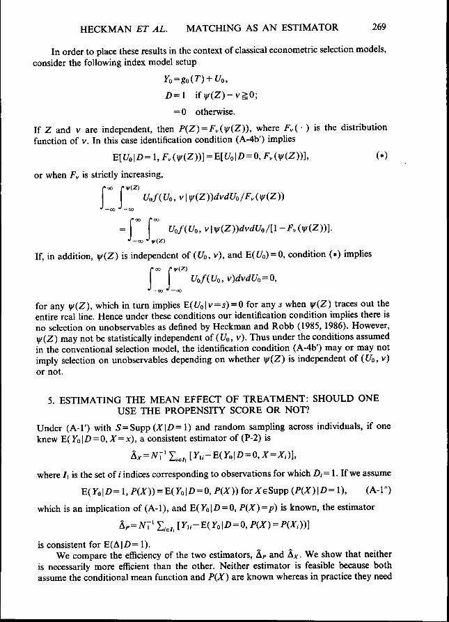
In order to place these results in the context of classical econometric selection models,consider the following index model setup
£>=1
= 0 otherwise.
If Z and V are independent, then P(Z) = F^(v/(Z)), where Fv( • ) is the distributionfunction of v. In this case identification condition (A-4b') implies
or when F^ is strictly increasing,(* oo C >ii(Z)LL
= \ I UoJ-oo •'v(Z)
If, in addition, y/iZ) is independent of (f/o, v), and E(f/o) = 0, condition (*) implies
Uo, v)dvdUo=0,(•oo I'V
for any v(Z), which in turn implies EiUo\v = s) = O for any 5 when v^(Z) traces out theentire real line. Hence under these conditions our identification condition implies there isno selection on unobservables as defined by Heckman and Robb (1985, 1986). However,ilfiZ) may not be statistically independent of (f/o, v). Thus under the conditions assumedin the conventional selection model, the identification condition (A-4b') may or may notimply selection on unobservables depending on whether y/iZ) is independent of (Co, v)or not.
5. ESTIMATING THE MEAN EFFECT OF TREATMENT: SHOULD ONEUSE THE PROPENSITY SCORE OR NOT?
Under (A-l') with S=SuppiX\D = \) and random sampling across individuals, if oneknew EiYo\D = 0,X=x), a consistent estimator of (P-2) is
where /i is the set of / indices corresponding to observations for which D, = 1. If we assume
E(yol^=l,i'(A')) = E(yo|Z> = 0,P(^))forZ6Supp(/ '(^)|Z)=l), (A-l")
which is an implication of (A-l), and E(rol^ = O, PiX)=p) is known, the estimator
is consistent for E(A|D= 1).We compare the efficiency of the two estimators, Ap and Ax. We show that neither
is necessarily more efficient than the other. Neither estimator is feasible because bothassume the conditional mean function and PiX) are known whereas in practice they need

270 REVIEW OF ECONOMIC STUDIES
to be estimated. However, the analysis of this case is of interest because the basic intuitionfrom the simple theorem established below continues to hold when the conditional meanfunction and P{X) are estimated.
Theorem 1. Assume:
(i) (A-l') and (A-l") hotdfor 5=Supp {X\D= 1);(ii) {^li,-^1 }/6/, cire independent and identicatty distributed;
and(iii) 0<E(F?) E(y?)<oo.
Then Kx and Ap are both consistent estimators of (P-2) with asymptotic distributionsthat are normat with mean 0 and asymptotic variances Vx and Vp, respectively, where
(r , |/)= 1, ^ ) |Z)= 1]-H Var [E(y, - ro|/)= 1, A')|Z)= 1],
and
|Z)= 1,/>(X))|£>= 1]-^ Var [E(r, - ro|/)= 1, P(Z))|Z)= 1].
The theorem directly follows from the central limit theorem for iid sampling withfinite second moment and for the sake of brevity its proof is deleted.
Observe that
E[Var (F, |£)= 1,Z)|D= l]^E[Var ( r , |/)= 1, i>(Z))|Z)= 1],
because X is in general a better predictor than P{X) but
Var [E(y, - Y^\D= \,X)\D= 1]^ Var [El(y, - Yo) \D^\, P{X)) \D= 1],
because vector X provides a finer conditioning variable than P{X). In general, there areboth costs and benefits of conditioning on a random vector X rather than P{X). Usingthis observation, we can construct examples both where F^g Vp and where K - Vp.
Consider first the special case where the treatment effect is constant, that isE{Yi-Yo\D=\,X) is constant. An iterated expectation argument implies thatE(y| - yo|Z)= 1, P{X)) is also constant. Thus, the first inequality, F^-g Vp holds in thiscase. On the other hand, if Yx = m{P{X)) + U for some measurable function m{ ) and £/and X are independent, then
which is non-negative because vector X provides a finer conditioning variable than P{X).So in this case Vx^Vp.
When the treatment effect is constant, as in the conventional econometric evaluationmodels, there is only an advantage to conditioning on X rather than on P{X) and thereis no cost.'" When the outcome 7, depends on X only through P(X), there is no advantageto conditioning on X over conditioning on P(X).
Thus far we have assumed that P(X) is known. In the next section, we investigatethe more realistic situation where it is necessary to estimate both P{X) and the conditional
10. Heckman (1992), Heckman and Smith (1998) and Heckman, Smith and Clements (1997) discuss thecentral role ofthe homogeneous response assumption in conventional econometric models of program evaluation.
HECKMAN ET AL. MATCHING AS AN ESTIMATOR 271
means. In this more realistic case, the trade-off between the two terms in Vx and Vppersists."
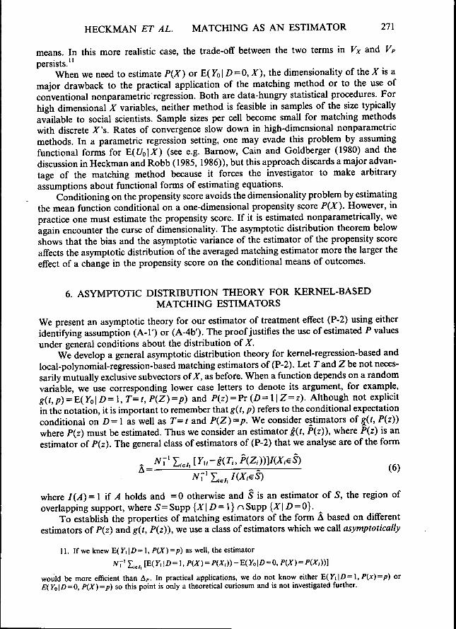
When we need to estimate P{X) or E(yo| Z) = 0, X), the dimensionality of the is amajor drawback to the practical application of the matching method or to the use ofconventional nonparametric regression. Both are data-hungry statistical procedures. Forhigh dimensional X variables, neither method is feasible in samples of the size typicallyavailable to social scientists. Sample sizes per cell become small for matching methodswith discrete A"s. Rates of convergence slow down in high-dimensional nonparametricmethods. In a parametric regression setting, one may evade this problem by assumingfunctional forms for E(t/o|A') (see e.g. Barnow, Cain and Goldberger (1980) and thediscussion in Heckman and Robb (1985, 1986)), but this approach discards a major advan-tage of the matching method because it forces the investigator to make arbitraryassumptions about functional forms of estimating equations.
Conditioning on the propensity score avoids the dimensionality problem by estimatingthe mean function conditional on a one-dimensional propensity score P{X). However, inpractice one must estimate the propensity score. If it is estimated nonparametrically, weagain encounter the curse of dimensionality. The asymptotic distribution theorem belowshows that the bias and the asymptotic variance of the estimator of the propensity scoreaffects the asymptotic distribution of the averaged matching estimator more the larger theeffect of a change in the propensity score on the conditional means of outcomes.
6. ASYMPTOTIC DISTRIBUTION THEORY FOR KERNEL-BASEDMATCHING ESTIMATORS
We present an asymptotic theory for our estimator of treatment effect (P-2) using eitheridentifying assumption (A-l') or (A-4b'). The proof justifies the use of estimated P valuesunder general conditions about the distribution of X.
We develop a general asymptotic distribution theory for kemel-regression-based andlocal-polynomial-regression-based matching estimators of (P-2). Let Tand Z be not neces-sarily mutually exclusive subvectors of , as before. When a function depends on a randomvariable, we use corresponding lower case letters to denote its argument, for example,g(,t,p) = E{Yo\D=\, T=t,P{Z)=p) and P(z) = Pr (D= 1 |Z=z). Although not explicitin the notation, it is important to remember that g{t, p) refers to the conditional expectationconditional on Z)= 1 as well as T=t and P(Z)=p. We consider estimators of g(r, i'(z))where P{z) must be estimated. Thus we consider an estimator g^t, P{z)), where P{z) is anestimator of Piz). The general class of estimators of (P-2) that we analyse are of the form
^ NT'L.,[Yu-giTi,PiZd)]IiXieS)^•^'' ( 6 )
where I{A) = l if A holds and =0 otherwise and S is an estimator of S, the region ofoverlapping support, where S = Supp {X\D=\}r\Supp {X\D = O}. ^
To establish the properties of matching estimators of the form K based on differentestimators of P(z) and g{t, Piz)), we use a class of estimators which we call asymptotically
11. If we knew E( y, | Z) = 1, P(X )=p)as well, the estimator
would be more efficient than Ap. In practical applications, we do not know either E(Yi\D=\,P{x)=p) orE{Yo\D = 0, P(X)=p) so this point is only a theoretical curiosum and is not investigated further.
272 REVIEW OF ECONOMIC STUDIES
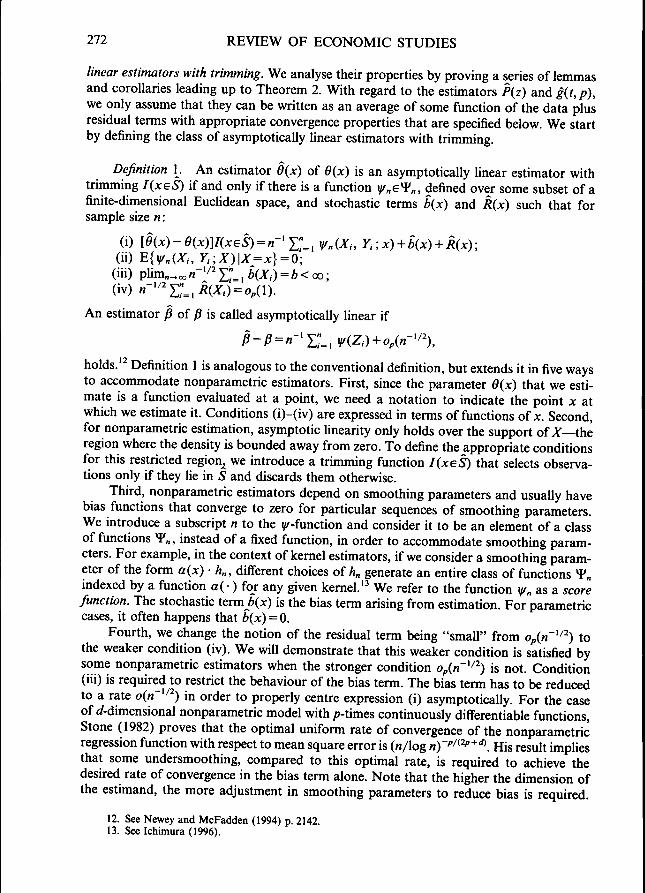
linear estimators with trimming. We analyse their properties by proving a series of lemmasand corollaries leading up to Theorem 2. With regard to the estimators P(z) and git,p),we only assume that they can he written as an average of some function of the data plusresidual terms with appropriate convergence properties that are specified below. We startby defining the class of asymptotically linear estimators with trimming.
Definition L An estimator Oix) of Oix) is an asymptotically linear estimator withtrimming IixeS) if and only if there is a function y/„£"¥„, defined over some subset of afinite-dimensional Euclidean space, and stochastic terms Six) and Rix) such that forsample size n:
(i) [9ix)-9ix)]IixeS) = n-' Yl^^ ^|/„iXi, Yr,x) + Six(ii) E{yf„iXl,Yr,X)\X=x} = O•,(iii) p\im„^^n-'/^X"=, KX,) = b<oo;
An estimator ^ of )3 is called asymptotically linear if
holds.'^ Definition 1 is analogous to the conventional definition, hut extends it in five waysto accommodate nonparametric estimators. First, since the parameter Oix) that we esti-mate is a function evaluated at a point, we need a notation to indicate the point x atwhich we estimate it. Conditions (i)-(iv) are expressed in terms of functions of x. Second,for nonparametric estimation, asymptotic linearity only holds over the support of X—theregion where the density is hounded away from zero. To define the appropriate conditionsfor this restricted region^ we introduce a trimming function IixeS) that selects ohserva-tions only if they lie in S and discards them otherwise.
Third, nonparametric estimators depend on smoothing parameters and usually havebias functions that converge to zero for particular sequences of smoothing parameters.We introduce a subscript n to the ^-function and consider it to he an element of a classof functions ^n, instead of a fixed function, in order to accommodate smoothing param-eters. For example, in the context of kernel estimators, if we consider a smoothing param-eter of the form ai^x) • hn, different choices of /»„ generate an entire class of functions H'nindexed hy a function c( •) for any given kernel." We refer to the function Vn as a scorefunction. The stochastic tenn^^(j:) is the hias term arising from estimation. For parametriccases, it often happens that Z>(jc) = O.
Fourth, we change the notion of the residual term heing "small" from Op(/i~' ) tothe weaker condition (iv). We will demonstrate that this weaker condition is satisfied hysome nonparametric estimators when the stronger condition 0;,(n~' ) is not. Condition(iii) is required to restrict the behaviour of the hias term. The hias term has to be reducedto a rate o(« ' ) in order to properly centre expression (i) asymptotically. For the caseof rf-dimensional nonparametric model with/?-times continuously differentiable functions.Stone (1982) proves that the optimal uniform rate of convergence of the nonparametricregression function with respect to mean square error is («/log n)'''^^^'''"^. His result impliesthat some undersmoothing, compared to this optimal rate, is required to achieve thedesired rate of convergence in the hias term alone. Note that the higher the dimension ofthe estimand, the more adjustment in smoothing parameters to reduce bias is required.
12. See Newey and McFadden (1994) p. 2142.13. See Ichimura (1996).

HECKMAN ET AL. MATCHING AS AN ESTIMATOR 273
This is the price that one must pay to safeguard against possible misspecifications of g(?, p)or Piz). It is straightforward to show that parametric estimators of a regression functionare asymptotically linear under some mild regularity conditions. In the Appendix weestablish that the local polynomial regression estimator of a regression function is alsoasymptotically linear.
A typical estimator of a parametric regression function mix; P) takes the formw(x; P), where m is a known function and P is an asymptotically linear estimator, with
^ n''^^^). In this case, by a Taylor expansion.
, P)-mix, p)] = n-'/' Y.%, [dmix, p)/8pWiX,, 7,)
+ [dmix, P)/dp-8mix, '
where P lies on a line segment between P and p. When E{ii/iXi, Yi)}=0 andE{\i/iXi, Yi){i/iXi, Y,)'}<oo, under iid sampling, for example, n~' ^EJ=i ViXi, Yi) =Opil) and plim„^o,p = P so that p\imr,^^\dmix, P)/dp-dmix, P)/8p\=0j,il) ifdmix, P)/dp is Holder continuous at p.^*
Under these regularity conditions
^[mix, p)-mix, )3)] = «-•/'X-=, [^'«(^' P)/8PMX,, y,) + o^(l).
The bias term of the parametric estimator mix, P) is Six) = 0, under the conditions wehave specified. The residual term satisfies the stronger condition that is maintained in thetraditional definition of asymptotic linearity.
(a) Asymptotic linearity of the kernel regression estimator
We now establish that the more general kernel regression estimator for nonparametricfunctions is also asymptotically linear. Corollary 1 stated below is a consequence of amore general theorem proved in the Appendix for local polynomial regression modelsused in Heckman, Ichimura, Smith and Todd (1998) and Heckman, Ichimura and Todd(1997). We present a specialized result here to simplify notation and focus on main ideas.To establish this result we first need to invoke the following assumptions.
Assumption 1. Sampling of {Xi, 7,} is i.i.d., X, takes values in R!' and F, in R, andVar(y,)<oo.
When a function is />-times continuously differentiable and its p-th derivative satisfiesHolder's condition, we call the function/7-smooth. Let mix) = E{Yi\Xi=x}.
Assumption 2. mix) is -smooth, where p>d.
14. A function is Holder continuous at A'=xo with constant 0< a g 1 if |q^x, 0) - (p{xo, fl)| g C • \\x-Xo\\°for some C> 0 for all x and 0 in the domain of the function cp(-,-). Usually Holder continuity is defined fora function with no second argument B. We assume that usual Holder continuity holds uniformly over 0 wheneverthere is an additional argument.
274 REVIEW OF ECONOMIC STUDIES
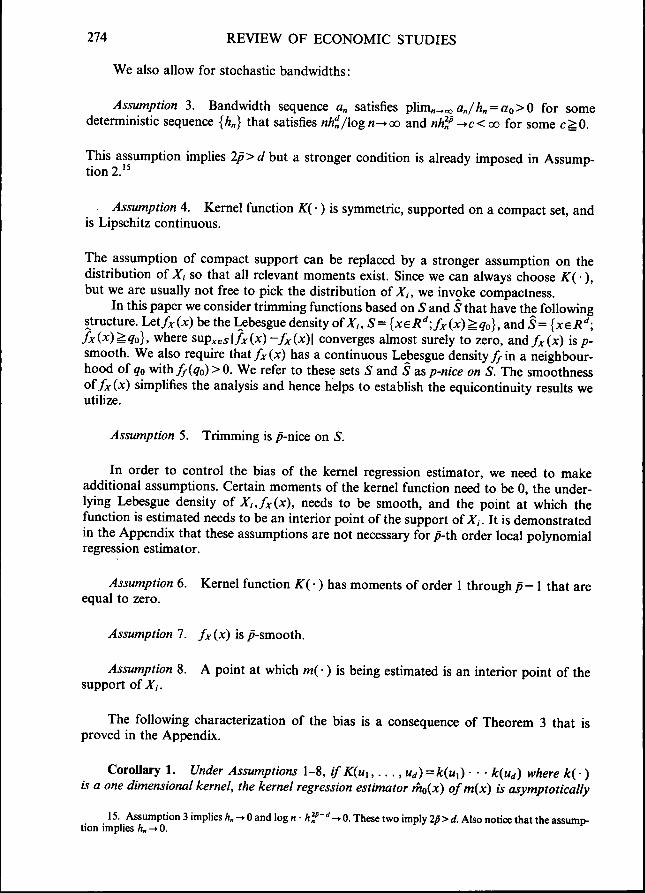
We also allow for stochastic bandwidths:
Assumption 3. Bandwidth sequence a, satisfies p\im„^^a„/h„ = ao>0 for somedeterministic sequence {h„} that satisfies nh^/logn-yao and nhf-*c<ao for some c^O.
This assumption implies 2^>rf but a stronger condition is already imposed in Assump-tion 2.'^
Assumption 4. Kernel function ^( •) is symmetric, supported on a compact set, andis Lipschitz continuous.
The assumption of compact support can be replaced by a stronger assumption on thedistribution of Xi so that all relevant moments exist. Since we can always choose Ki •),but we are usually not free to pick the distribution of Z,, we invoke compactness.
In this paper we consider trimming functions based on S and S that have the followingstructure. hQifxix) be the Lebesgue density oiX,, S= {xeR'';fxix)^qo}, and S= {xeR'';fxix)^qo}, where supxes\fxix)-fxix)\ converges almost surely to zero, and/;i-(jc) isp-smooth. We also require that fxix) has a continuous Lebesgue density j | ^ in a neighbour-hood of qo vnthffiqo) > 0. We refer to these sets S and S as p-nice on S. The smoothnessof fxix) simplifies the analysis and hence helps to establish the equicontinuity results weutilize.
Assumption 5. Trimming is ^-nice on S.
In order to control the bias of the kernel regression estimator, we need to makeadditional assumptions. Certain moments of the kernel function need to be 0, the under-lying Lebesgue density of Xt,fxix), needs to be smooth, and the point at which thefunction is estimated needs to be an interior point ofthe support of Z,. It is demonstratedin the Appendix that these assumptions are not necessary for ^-th order local polynomialregression estimator.
Assumption 6. Kernel function Ki •) has moments of order 1 through p - 1 that areequal to zero.
Assumption!. />(:>(:) is -smooth.
Assumption 8. A point at which m(-) is being estimated is an interior point of thesupport of A',.
The following characterization of the bias is a consequence of Theorem 3 that isproved in the Appendix.
CoroUary 1. Under Assumptions 1-8, if Kiu^,..., Ud)=kiui) • • • kiuj) where ki •)is a one dimensional kernel, the kernel regression estimator rhoix) of mix) is asymptotically
15. Assumption 3 implies />„ -• 0 and log n • A ^ "'' -• 0. These two imply 2p > d. Also notice that the assump-tion implies K-^O.
HECKMAN ET AL. MATCHING AS AN ESTIMATOR 275
linear with trimming., where, writing e,= Yi-B{Yi\Xi}, and
Wn(.Xi, Yi • x) = (naohi)-'EiKi{Xi-x)/iaohr.))r{xeS)/fx(x),
Six) =
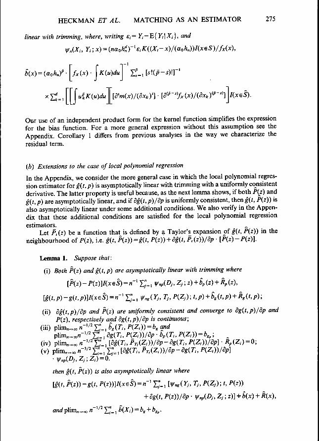
Our use of an independent product form for the kernel function simplifies the expressionfor the bias function. For a more general expression without this assumption see theAppendix. Corollary 1 differs from previous analyses in the way we characterize theresidual term.
(b) Extensions to the case of local polynomial regression
In the Appendix, we consider the more general case in which the local polynomial regres-sion estimator for g(t, p) is asymptotically linear with trimming with a uniformly cqiisistentderivative. The latter property is useful because, as the next lemma shows, if both P{z) andg{t, p) are asymptotically linear, and if dg^t, p)/dp is uniformly consistent, then g^t, P(z)) isalso asymptotically linear under some additional conditions. We also verify in the Appen-dix that these additional conditions are satisfied for the local polynomial regressionestimators.
Let P,(z) be a function that is defined by a Taylor's expansion pf i(r, P(z)) in theneighbourhood of P(z), i.e. g{t, P(,z))=g(,t, P(z)) + dg(t, P,(z))/dp • [P(z)-P{z)l
Lemma 1. Suppose that:
(i) Both P(z) andg(t,p) are asymptotically linear with trimming where
(ii) dg(t,p)/dp and P(z) are uniformly consistent and converge to dg{t,p)/dp andP(z), respectively and dg(t,p)/dp is continuous;
(iii) plim„-.oo «"'/' i ; - , S,(T,, P(Z,)) = b, andplim«^««-'/' i ;_, 8g(Ti, PiZ,))/8p • b,iT,, P(Z,)) = b,^; ^
(iv) plim .oo «"'^' Z;-, lSg(T>, PT.iZi))/Sp-8g(Ti, P(Z,))/8p](V) plim^^^ n-'^' i ;^ , i ; 8 d i j P{Zd)/
then g(t, P{z)) is also asymptotically linear where
[g(t, Piz))-g{t, PizW(xeS) = n-' S;=, IVnAYj, Tj, P{Zj); t, P(z))
+ dgit, P(z))/dp • yifnp^Dj, Zj; z)] -I-b{x) + R{x),
andli ~' ^ Z" MX)

276 REVIEW OF ECONOMIC STUDIES
An important property of this expression which we exploit below is that the effect ofthe kernel function v n CA, 'Zj\'^) always enters multiplicatively with dg{t, P{z))/dp. Thusboth the bias and variance of P{z) depend on the slope to g with respect to p. Condition(ii) excludes nearest-neighbour type matching estimators with a fixed number of neigh-bours. With conditions (ii)-(v), the proof of this lemma is just an application of Slutsky'stheorem and hence the proof is omitted.
In order to apply the theorem, however, we need to verify the conditions. We sketchthe main arguments for the case of parametric estimator P(z) of P{z) here and presentproofs and discussion of the nonparametric case in the Appendix.^ Under the regularity conditions just presented, the bias function for a parametricP{z) is zero. Hence condition (iii) holds '\fg(,t,p) is asymptotically linear and its derivativeis uniformly consistent for the true derivative. Condition (iv) also holds since \Rp{Z,) | =Op {n '/^) and the derivative oig{t, p) is uniformly consistent. Condition (v) can be verifiedby exploiting the particular form of score function obtained earlier. Observing thatW{D Z; Z) v ' ( Z ) WpiiDj, Zf), we obtain
, P{Zi))/dp]
g(Ti, P{Zi))/dp]xifp,{Zi)n-''^ Y.%, VpiiDj, Zj),
so condition (v) follows from an application of the central limit theorem and the uniformconsistency of the derivative of g(t,p).
For the case of nonparametric estimators, Vnp does not factor and the double summa-tion does not factor as it does in the case of parametric estimation. For this more generalcase, we apply the equicontinuity results obtained by Ichimura (1995) for general U-statistics to verify the condition. We verify all the conditions for the local polynomialregression estimators in the Appendix. Since the derivative of g{t,p) needs to be definedwe assume
Assumption 9. K() is 1-smooth.
Lemma 1 implies that the asymptotic distribution theory of A can be obtained forthose estimators based on asymptotically linear estimators with trimming for the generalnonparametric (in P and g) case. Once this result is established, it can be used with lemma1 to analyze the properties of two stage estimators of the form g(t, P(z)).
(c) Theorem 2: The asymptotic distribution of the matching estimator under generalconditions
Theorem 2 enables us to produce the asymptotic distribution theory of a variety of estima-tors A of the treatment effect under different identifying assumptions. It also produces theasymptotic distribution theory for matching estimators based on different estimators ofg(t,p) and P(z). In Sections 3 and 4, we presented various matching estimators for themean effect of treatment on the treated invoking different identifying assumptions. Analtemative to matching is the conventional index-sufficient selection estimators that canbe used to construct estimators of E (yo|/)= 1, A ), as described in our companion paperHeckman, Ichimura and Todd (1997) and in Heckman, Ichimura, Smith and Todd(1996a, 1998). Our analysis is sufficiently general to cover the distribution theory for thatcase as well provided an exclusion restriction or a distributional assumption is invoked.

HECKMAN ET AL. MATCHING AS AN ESTIMATOR 277
Denote the conditional expectation or variance given that A' is in S by Es ( ) orVar5( ), respectively. Let the number of observations in sets h and h be No and N\,respectively, where N=No + N^ and that 0<limAr_oo Ni/No=0<co.
Theorem 2. Under the following conditions:(i) {yo,, Xi },e/o and {Yu, A', },e/, are independent and within each group they are i.i.d.
and Yoi for ielo and Yufor ielx each has a finite second moment;(ii) The estimator g{x) of g{x) = {Yo\Di=\,Xi=x] is asymptotically linear with
trimming., where
Mix)-g{x)]I{xeS} = No' !, , ,„ ^foN^sX J'o,,Xi; x)
and the score functions y/dNoN,(Yd,X; x) for d=0 and 1, the bias term bgix), andthe trimming function satisfy:
(ii-a) E {Vrf vo^v,(y</MXi;X)\Di = d,X,D=\)}=Ofor d=0 and 1, andVar {ii/ciNoNXYdi,Xi •,X)} = oiN) for each ielou/, ;
(ii-b) pUm^v. co A^r'^' I , , , , kXi) = b;(ii-c) plim , <:o Var {E[y/oNoNXYo>,Xi;X)\ Yoi, Di = O,Xi,D=l]|/>= 1} = Ko<oo
plim^v. oo Var {E[y/,!,,^,iYu, Xi; X) \ Yu, Di= 1, Xi, D= 1] |Z)= 1} = K, < co,andlim^v. co E{[Yu-giXi)]IiXieS) •
lXD(ii-d) S and S are p-nice on S, where p>d, where d is the number of regressors in X
and fix) is a kernel density estimator that uses a kernel function that satisfiesAssumption 6.
Then under (A-T) the asymptotic distribution of
is normal with mean ib/Pr iXeS\D=l)) and asymptotic variance
YAT, PiZ), D=
+ PriXeS\D=l)-^{V,+2-
Proof. See the Appendix.
Theorem 2 shows that the asymptotic variance consists of five components. The firsttwo terms are the same as those previously presented in Theorem 1. The latter three termsare the contributions to variance that arise from estimating gix) = E{Yi\Di=l,Xi=x}.The third and the fourth terms arise from using observations for which D = 1 to estimategix). If we use just observations for which D = 0 to estimate gix), as in the case of thesimple matching estimator, then these two terms do not appear and we only acquire the
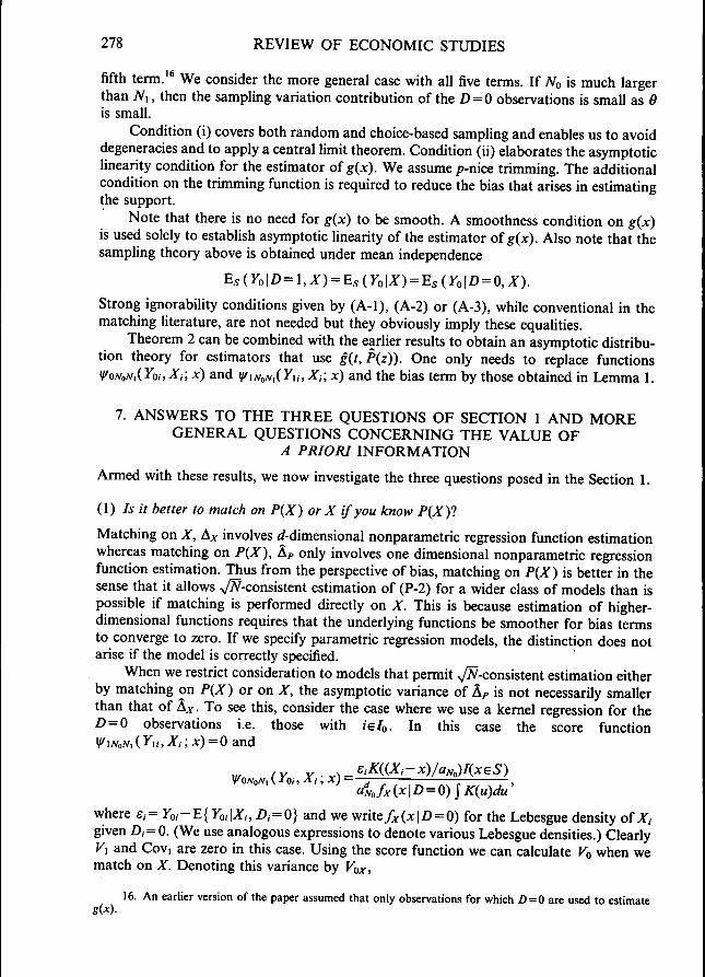
278 REVIEW OF ECONOMIC STUDIES
fifth term.'* We consider the more general case with all five terms. If Ao is much largerthan AT,, then the sampling variation contribution of the Z) = 0 observations is small as 6is small.
Condition (i) covers both random and choice-based sampling and enables us to avoiddegeneracies and to apply a central limit theorem. Condition (ii) elaborates the asymptoticlinearity condition for the estimator of gix). We assume/7-nice trimming. The additionalcondition on the trimming function is required to reduce the bias that arises in estimatingthe support.
Note that there is no need for gix) to be smooth. A smoothness condition on gix)is used solely to establish asymptotic linearity of the estimator of gix). Also note that thesampling theory above is obtained under mean independence
Strong ignorability conditions given by (A-l), (A-2) or (A-3), while conventional in thematching literature, are not needed but they obviously imply these equalities.
Theorem 2 can be combined with the earlier results to obtain an asymptotic distribu-tion theory for estimators that use git, Piz)). One only needs to replace functions
iYoi>Xi; x) and iifiN^XYuyXr, x) and the bias term by those obtained in Lemma 1.
7. ANSWERS TO THE THREE QUESTIONS OF SECTION 1 AND MOREGENERAL QUESTIONS CONCERNING THE VALUE OF
A PRIORI INFORMATION
Armed with these results, we now investigate the three questions posed in the Section 1.
il) Is it better to match on PiX) or X if you know
Matching on X, Ax involves ^-dimensional nonparametric regression function estimationwhereas matching on PiX), Kp only involves one dimensional nonparametric regressionfunction estimation. Thus from the perspective of bias, matching on PiX) is better in thesense that it allows ^A^-consistent estimation of (P-2) for a wider class of models than ispossible if matching is performed directly on X. This is because estimation of higher-dimensional functions requires that the underlying functions be smoother for bias termsto converge to zero. If we specify parametric regression models, the distinction does notarise if the model is correctly specified.
When we restrict consideration to models that permit >/F-consistent estimation eitherby matching on PiX) or on X, the asymptotic variance of Kp is not necessarily smallerthan that of Kx. To see this, consider the case where we use a kernel regression for theD = 0 observations i.e. those with ielo. In this case the score function
w (Y . . . , • ^ _WONoN, ( -fOl, ^i , X)
where £,= yo,-E{ I'o/IA',, A = 0} and we write/A-(x|Z) = O) for the Lebesgue density of X,given Z), = 0. (We use analogous expressions to denote various Lebesgue densities.) ClearlyV] and Covi are zero in this case. Using the score function we can calculate Ko when wematch on X. Denoting this variance by Vox,
16. An earlier version ofthe paper assumed that only observations for which £) = 0 are used to estimate8(x).

HECKMAN ET AL. MATCHING AS AN ESTIMATOR 279
M ' J J
Now observe that conditioning on Xi and Fo,, e, is given, so that we may write the lastexpression as
I r^((^r:^)^^^Mf^ 1 ijr UjxiX\D = O)JKiu)du^ J' I
Now
r/.((X-^)/a.)/(X.5) 1d' j
can be written in the following way, making the change of variable iX/-
aNoW\D = 0)
Taking limits as No-^oa, and using assumptions 3, 4 and 7, so we can take limits insidethe integral
since OATO^O and ^Kiw)dw/lKiu)du= 1. Thus, since we sample the Xi for which A = 0,
L ./A-(. /IM —"J
Hence the asymptotic variance of AA- is, writing A=Pr {A'e5|Z) = 0}/Pr (.YeS'|£)= 1),
Pr iXeS\D = l)-'{YaTs [EsiY,- Yo\X, D= 1)\D= l] + Es[Vars(F, \X, Z)=
Similarly for Ap, VOP is
The first two terms for both variance expressions are the same as those that appear in Vxand Vp in Theorem 1. To see that one variance is not necessarily smaller than the other,consider the case where fxiX\D=l)=fxiX\D = O) and 9 = 1. Clearly in this casefpiPiX)\D= l)=fpiPiX)\D = O). Propensity score matching has smaller variance if and
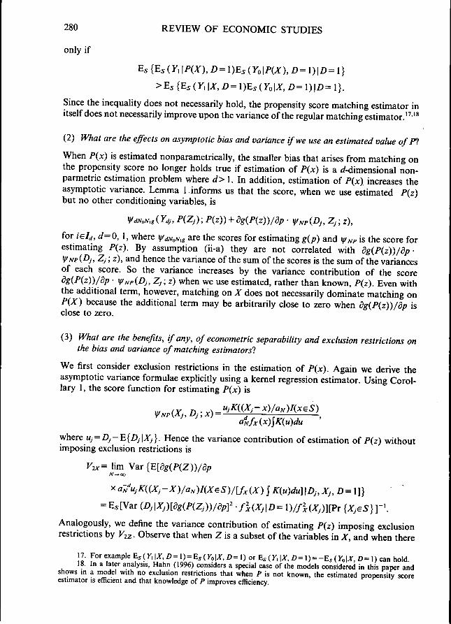
280 REVIEW OF ECONOMIC STUDIES
only if
Es{EsiY,\PiX),D=l)EsiYo\PiX),D=l)\D=l}
>Es{EsiYt\X,D=l)EsiYo\X,D=l)\D=\}.
Since the inequality does not necessarily hold, the propensity score matching estimator initself does not necessarily improve upon the variance ofthe regular matching estimator."'*
(2) What are the effects on asymptotic bias and variance if we use an estimated value of F>.
When Pix) is estimated nonparametrically, the smaller bias that arises from matching onthe propensity score no longer holds true if estimation of Pix) is a ^/-dimensional non-parmetric estimation problem where rf> 1. In addition, estimation of Pix) increases theasymptotic variance. Lemma 1. informs us that the score, when we use estimated Piz)but no other conditioning variables, is
for ieIj,d=O,\, where \i/dNoN,g are the scores for estimating gip) and IJ/NP is the score forestimating Piz). By assumption (ii-a) they are not correlated with dgiPiz))/8p-WspiDj, Zj; z), and hence the variance ofthe sum ofthe scores is the sum ofthe variancesof each score. So the variance increases by the variance contribution of the scoreSgiPiz))/dp • y/NpiDj, Zjiz) when we use estimated, rather than known, Piz). Even withthe additional term, however, matching on X does not necessarily dominate matching onPiX) because the additional term may be arbitrarily close to zero when dgiPiz))/8p isclose to zero.
(3) What are the benefits, if any, of econometric separability and exclusion restrictions onthe bias and variance of matching estimators?
We first consider exclusion restrictions in the estimation of Pix). Again we derive theasymptotic variance formulae explicitly using a kernel regression estimator. Using Corol-lary 1, the score function for estimating Pix) is
a%fxix)\Kiu)du '
uj=Dj-E{Dj\Xj}. Hence the variance contribution of estimation of Piz) withoutimposing exclusion restrictions is
V2x= lim y&r{E[dgiPiZ))/dpN*co
Kiu)du]\Dj,Xj,D=l]}
iDj\Xj)[dgiPiZj))/dp]' -fliXjlD^ l)/f%iXj)][PT {XjeS}]-\
Analogously, we define the variance contribution of estimating P(z) imposing exclusionrestrictions by Viz. Observe that when Z is a subset of the variables in X, and when there
17. FoTexamp\eEs(Y,\X,D\) Es{Yo\X,D=\)oTEs(Y,\X,D=\) = -Es(Yo\X,D=\)ainho\d.18. In a later analysis, Hahn (1996) considers a special case of the models considered in this paper and
shows in a model with no exclusion restrictions that when P is not known, the estimated propensity scoreestimator is efficient and that knowledge of P improves efficiency.

HECKMAN ET AL. MATCHING AS AN ESTIMATOR 281
are exclusion restrictions so PiX) = PiZ) then one can show that V2zS Vix- Thus, exclu-sion restrictions in estimating PiX) reduce the asymptotic variance of the matching estima-tor—an intuitively obvious result.
To show this first note that in this case Var (D|^) = Var (/)|Z). Thus
iD\Z)[dgiPiZ))/8pf
= 0.
Since the other variance terms are the same, imposing the exclusion restriction helps toreduce the asymptotic variance by reducing the estimation error due to estimating thepropensity score. The same is true when we estimate the propensity score by a parametricmethod. It is straightforward to show that, holding all other things constant, the lowerthe dimension of Z, the less the variance in the matching estimator. Exclusion restrictionsin T also reduce the asymptotic variance of the matching estimator.
By the same argument, it follows that E{[f%iX\D=l)/fJciX\D = O)] - 1 |D = 0} ^0 .This implies that under homoskedasticity for Fo, the case/(A'|Z)= l)=/(X|£> = 0) yieldsthe smallest variance.
We next examine the consequences of imposing an additive separability restrictionon the asymptotic distribution. We find that imposing additive separability does not neces-sarily lead to a gain in efficiency. This is so, even when the additively separable variablesare independent. We describe this using the estimators studied by Tjostheim and Auestad(1994) and Linton and Nielsen (1995)."
They consider estimation of fi(^i),g2(A'2) in
where x = (xi, X2). There are no overlapping variables among Xi and X2. In our context,E( Y\X = x)=git) + KiPiz)) and EiY\X=x) is the parameter of interest. In order to focuson the effect of imposing additive separability, we assume /'(z) to be known so that wewrite P for/'(Z).
Their estimation method first estimates E{Y\T=t,P=p}=git) +Kip) non-para-metrically, say by fi {y| T= t, P=p}, and then integrates £ { y| 7= /, P=p} over p usingan estimated marginal distribution of P. Denote the estimator by git). Then under additiveseparability, git) consistently estimates git)+ E{KiP)}. Analogously one can integratefi { y| T= t, P=p] —git) over t using an estimated marginal distribution of T to obtain aconsistent estimator of Kip)-E{KiP)). We add the estimators to obtain the estimatorof EiY\X=x) that imposes additive separability. The contribution of estimation of theregression function to asymptotic variance when T and P are independent and additive
19. The derivative of E{ Y\T=t, P=p) with respect to p only depends on p if it is additively separable.Fan, Hardle and Mammen (1996) exploits this property in their estimation. Using this estimator does not leadto an improvement in efficiency, either.
282 REVIEW OF ECONOMIC STUDIES
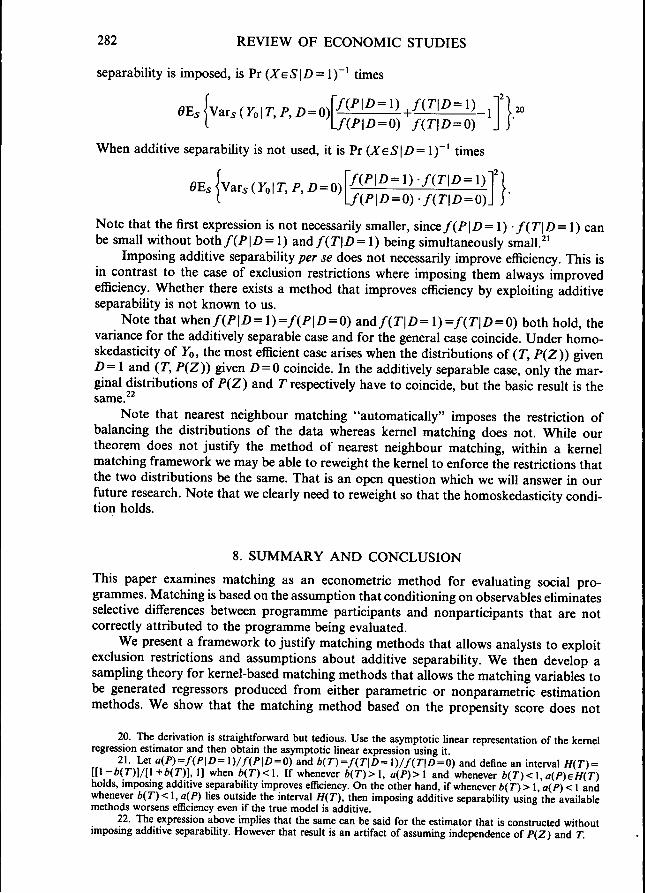
separability is imposed, is Pr iXeS\D = l)~^ times
YolT, P, D =iP\D = O) fiT\D = O)
When additive separability is not used, it is Pr iXeS\D=l)~^ times
Note that the first expression is not necessarily smaller, since fiP\D= 1) •/(r|Z>= 1) canbe small without both/(P|Z)= 1) and fiT\D=l) being simultaneously small. '
Imposing additive separability per se does not necessarily improve efficiency. This isin contrast to the case of exclusion restrictions where imposing them always improvedefficiency. Whether there exists a method that improves efficiency by exploiting additiveseparability is not known to us.
Note that when/(P|Z)= 1)=/(P|D = O) andfiT\D= l )= / ( r |£ ) = O) both hold, thevariance for the additively separable case and for the general case coincide. Under homo-skedasticity of ^0, the most efficient case arises when the distributions of (r, PiZ)) givenD= 1 and (T, PiZ)) given D = 0 coincide. In the additively separable case, only the mar-ginal distributions of PiZ) and T respectively have to coincide, but the basic result is the
Note that nearest neighbour matching "automatically" imposes the restriction ofbalancing the distributions of the data whereas kernel matching does not. While ourtheorem does not justify the method of nearest neighbour matching, within a kernelmatching framework we may be able to reweight the kernel to enforce the restrictions thatthe two distributions be the same. That is an open question which we will answer in ourfuture research. Note that we clearly need to reweight so that the homoskedasticity condi-tion holds.
8. SUMMARY AND CONCLUSION
This paper examines matching as an econometric method for evaluating social pro-grammes. Matching is based on the assumption that conditioning on observables eliminatesselective differences between programme participants and nonparticipants that are notcorrectly attributed to the programme being evaluated.
We present a framework to justify matching methods that allows analysts to exploitexclusion restrictions and assumptions about additive separability. We then develop asampling theory for kernel-based matching methods that allows the matching variables tobe generated regressors produced from either parametric or nonparametric estimationmethods. We show that the matching method based on the propensity score does not
20. The derivation is straightforward but tedious. Use the asymptotic linear representation of the kernelregression estimator and then obtain the asymptotic linear expression using it
21. Let a(P)=f(P\D=l)/f{P\D = O) and b(T)=/{T\D=\)/f{T\D = O) and define an interval H(T) =[l\-b(T)]/[l+b(T)], 1] when b(T)<l. If whenever b(T)>\, a(P)>l and whenever b(T)<\,a{P)eHiT)holds, imposing additive separability improves efficiency. On the other hand, if whenever b(T)>l,a(P)<l andwhenever b(T)<\, a(P) lies outside the interval H(T), then imposing additive separability using the availablemethods worsens efficiency even if the true model is additive.
22. The expression above implies that the same can be said for the estimator that is constructed withoutimposing additive separability. However that result is an artifact of assuming independence of P(Z) and T.

HECKMAN ET AL. MATCHING AS AN ESTIMATOR 283
necessarily reduce the asymptotic bias or the variance of estimators of M(S) comparedto traditional matching methods.
The advantage of using the propensity score is simplicity in estimation. When we usethe method of matching based on propensity scores, we can estimate treatment effects intwo stages. First we build a model that describes the programme participation decision.Then we construct a model that describes outcomes. In this regard, matching mimicsfeatures of the conventional econometric approach to selection bias. (Heckman and Robb(1986) or Heckman, Ichimura, Smith and Todd (1998).)
A useful extension of our analysis would consider the small sample properties ofalternative estimators. In samples of the usual size in economics, cells will be small ifmatching is made on a high-dimensional X. This problem is less likely to arise whenmatching is on a single variable like P. This small sample virtue of propensity scorematching is not captured by our large sample theory. Intuitively, it appears that the lessdata hungry propensity score method would be more efficient than a high dimensionalmatching method.
Our sampling theory demonstrates the value of having the conditional distributionof the regressors the same for £> = 0 and D=\. This point is to be distinguished from therequirement of a common support that is needed to justify the matching estimator.Whether a weighting scheme can be developed to improve the asymptotic variance remainsto be investigated.
APPENDIX
In this Appendix we prove Corollary 1 by proving a more general result, Theorem 3 stated below, verify theconditions of Lemma 13, for the case of a local polynomial regression estimator, and prove Theorem 2. We firstestablish the property that local polynomial regression estimators are asymptotically linear with trimming.
A. 1. Theorem 3
Theorem 3 will show that local polynomial regression estimators are asymptotically linear with trimming. Lemma1 follows as a corollary.
The local polynomial regression estimator of a function and its derivatives is based on an idea of approxim-ating the function at a point by a Taylor's series expansion and then estimating the coefficients using data in aneighbourhood ofthe point. In order to present the results, therefore, we first develop a compact notation to writea multivariate Taylor series expansion. Let x = ( x i , . . . , x^) and 9 = ( 9 , , . . . , qd)eR'' where qj (j= 1 </) arenonnegative integers. Also let y = x?'.. .xy/(q^ ... qJ). Note that we include iq,<.... qjl) in the definition. Thisenables us to study the derivative of x' without introducing new notation; for example, 5x'/5xi =x* where q =(q,-\ qj), if gi S1 and 0 otherwise. When the sum of the elements of 9 is i, x* corresponds to a Taylorseries polynomial associated with the term d'm(x)/(dx^'... dx^J). In order to consider all polynomials thatcorrespond to i-th order derivatives we next define a vector whose elements are themselves distinct vectors ofnonnegative integers whose elements sum to .s. We denote this row vector by Q(s) = ({q],... ,qd))<,,+ ••+<,^-s',that is Q(s) is a row vector of length (s + d- \y./[s\(d-1)!] whose typical element is a row vector ( 9 , , . . . , qj),which has arguments that sum to .s. For concreteness we assume that {(q,,..., q^)} are ordered according tothe magnitude of ^f.., •O''"''?; from largest to smallest. We define a row vector x^''' = (x'" "'),, + ...+,^.,. Thisrow vector corresponds to the polynomial terms of degree j . Let x^' = (x'^''^),e{o.i...j,) • This row vector representsthe whole polynomial up to degree p from lowest to the highest.
Also let m'''(x) for s^\ denote a row vector whose typical element is 5'm(x)/(5x1f'... SxJ*) whereq, + - • •+qj=s and the elements are ordered in the same way {{q,,... ,qj)} are ordered. We also write m'°'(x) =m(x). Let P*(xo) = (m""(xo), • . . , m^\xo)y. In this notation, Taylor's expansion of m(x) at Xo to orderp withoutthe remainder term can now be written as (x-xo)^'^*(xo).
We now define the local polynomial regression estimator with a global smoothing parameter aA,, whereo e [ a o - 5 , a o + 5 ] f o r s o m e a o > 0 a n d a o > 5 > 0 . Wedenoteja^ = [ a o - 5 , a o + 5 ] . Let K|,{s) = {ah„)'''K(s/(ah„))and KM(S) = (aM'''. K(s/(aM), and let ^ = ( )8 i , . . . , P,)', where p', is conformable with m""(xo), for r = 0 p.

284 REVIEW OF ECONOMIC STUDIES
Also let y = ( y , , . . . , ¥„)', W(A:o) = diag (K,(X,-xo),..., K.iX^-xo)), and
Then the local polynomial regression estimator is defined as the solution to
or, more compactly
P,(xo) = arg min (Y-X^(xo)p)' fV(xo)( Y-X,(xo)P).
Clearly the estimator equals [X'p(xaW(xo)Xp(xo)Y'X'p{xa)W(xo)Y when the inverse exists. When /) = 0, theestimator is the kernel regression estimator and when/)= 1 the estimator is the local linear regression estimator."
Let //=diag (\,(aKyUj,..., (a/i,)"''i(;,+rf-i),/[;,t(rf-i,,,), where i, denotes a row vector of size s with 1 inall arguments. Then P,(x<,) = H[M,„{xor'\n''H•X',{x„)W{xo)Y, where M,Axa) = n-'WX;(xo)W(x<,)X,(xa)H.
Note that by Taylor's expansion of order p^p at Xo,m(X,) = (X,-Xn)°'P*{xo) + rf(X,,Xo), whererp(.Xi, Xa) = (X,-xo)^''\m'^\x,)-m^\xo)] and Xt lies on a line between X, and Xa. Write
W = (TO(X,), . . . , m(X„))•, r^(xo) = (r^(X,, ATo),..., r^(X„, Xo))', and e = (e^,..., e j ' .
Let M,«(xo) be the square matrix of size j ; ^ . ^ [{q + d- 1 )\/q\ (d- 1)!] denoting the expectation of / / ,„ (xo),where the j-th row, /-th column "block" of A/,»(;co) matrix is, for Og.s, r g p .
Let lim,^» M,„(xo) = M,•/(J»ro)''*^ Note that M^ only depends on K() when Xo is an interior point of thesupport of A-. Also write l = I{X,eS} and /, = /{X,65}, /o = /{A:oeS} and 1^ = 1 {xoeS}. We prove the followingtheorem.
Theorem 3. Suppose Assumptions 1-4 hold. If M^ is non-singular, then the local polynomial regressionestimator of order p, m^ix), satisfies
where 6(xo) = o(/i^),/i- '^'£;_, R(X,) = o^O), and
; Xo) = (l , 0 0)
Furthermore, suppose that Assumptions 5-7 hold. Then the local polynomial regression estimator of orderO^p<p ihpix), satisfies
where
Fan (1993), Ruppert and Wand (1994), and Masry (1995) prove pointwise or uniform convergence prop-erty^of the estimator. As for any other nonparametric estimator the convergence rate in this sense is slower thann -rate. We prove that the averaged pointwise residuals converges to zero faster than n"'^^-rate.
We only specify that M, is nonsingular because one can find different conditions on Ar( ) to guarantee it.For example, assuming that fC(u,,... ,uj)=k(u,)... k{uj), if J s'^k(s)ds > 0, then M, is nonsingular.
23. Ruppert and Wand (1994) develop multivariate version of the local linear estimator. Masry (1995)develops multivariate general order local polynomial regression.
HECKMAN ET AL. MATCHING AS AN ESTIMATOR 285
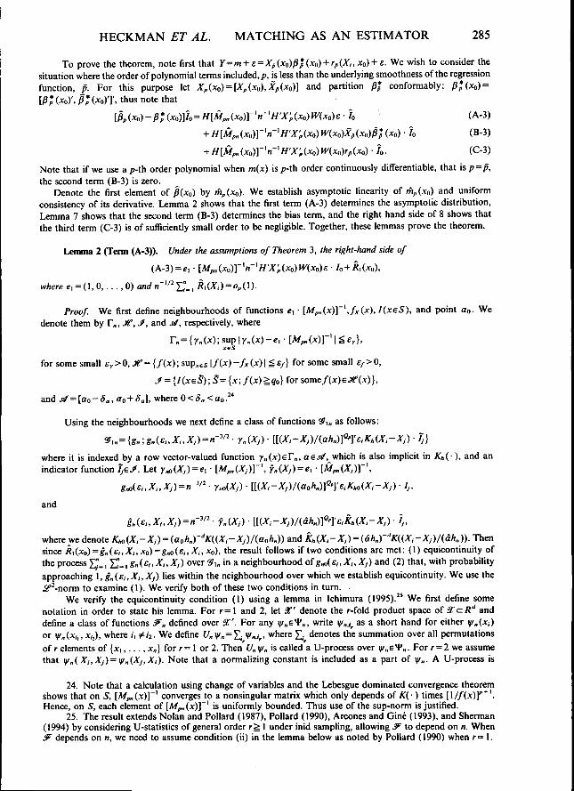
To prove the theorem, note first that Y=m+B=Xp{xa)P*(xo) + rp{X,,Xa) +e. We wish to consider thesituation where the order of polynomial terms included,/?, is less than the underlying smoothness of the regressionfunction, p. For this purpose let Xp(x,,) = [Xp(xQ),Xp(xo)'\ and partition p* conformably: P*(xo) =[^; (xo)', Pt (xo)T. thus note that
(A-3)
) • h (B-3)
(C-3)
Note that if we use a p-th order polynomial when m(x) is ;7-th order continuously differentiable, that is p=p,the second term (B-3) is zero.
Denote the first element of P{xo) by m^ixo). We establish asymptotic linearity of thpixo) and uniformconsistency of its derivative. Lemma 2 shows that the first term (A-3) determines the asymptotic distribution.Lemma 7 shows that the second term (B-3) determines the bias term, and the right hand side of 8 shows thatthe third term (C-3) is of sufficiently small order to be negligible. Together, these lemmas prove the theorem.
Lemma 2 (Term (A-3)). Under the assumptions of Theorem 3, the right-hand side of
(A-3) = e, • [M^(xo)Y'"~'H'X'p(X(,)W{xo)e • Io+R^Xa),
where e, = (1, 0 , . . . , 0) and n"'^' E"-, RAX,) = Op(\).
Proof We first define neighbourhoods of functions e, • [Mp„{x)Y\fx(x), l(xeS), and point Oo. Wedenote them by Tn, Jtf, J, and si, respectively, where
for some small e ,>0 , j r = {/(x);sup«sl/(Jc)-/A-(x)l £« /} for some small e />0,
J={l(x^S),S= {x; f{x)^qo} forsome/(A:)e.?r(jc)},
and J3 = [ff0-5o, ao + 5a], where O<Sa<ao.^*
Using the neighbourhoods we next define a class of functions ^ i , as follows:
where it is indexed by a row vector-valued function yn(x)ern, aeja^, which is also implicit in Ki,(), and anindicator function TjeJ. Let y^(Ay) = c, • [M,,(A'y)]-', y,(.^O) = e, • [ M \
and
J
since Ri(xa)=gn{ei,X,,xo)-gM(e,,X,,xo), the result follows if two conditions are met: (1) equicontinuity ofthe process I J . , S^., ?„(£,, X,,Xj) over ^ , , in a neighbourhood of ^^(e , , ^ , , Xj) and (2) that, with probabilityapproaching 1, §„(£,,X,,Xj) lies within the neighbourhood over which we establish equicontinuity. We use thejSf^-norm to examine (1). We verify both of these two conditions in tum.
We verify the equicontinuity condition (1) using a lemma in Ichimura (1995)." We first define somenotation in order to state his lemma. For r = 1 and 2, let 3C' denote the r-fold product space of 3^<=/?'' anddefine a class of functions i^» defined over SC'. For any v^e*?,, write v,./, as a short hand for either v,(x,)or i^n(x,,, x,j), where ii ?ti2. We define {/„ Vn = l]j V'n.*,. where X, denotes the summation over all permutationsof r elements of {xi , . . . ,Xn} f o r r = l or 2. Then {/„ Vn is called a U-process over (f/nST,. For r = 2 we assumethat \^n(Xi,Xj)=\yn(Xj,X,). Note that a normalizing constant is included as a part of v'n- A U-process is
24. Note that a calculation using change of variables and the Lebesgue dominated convergence theoremshows that on 5, [A/,n(x)]~' converges to a nonsingular matrix which only depends of K(-) times [l / /( .x)l '* ' .Hence, on S, each element of [Mp,,(x)Y^ is uniformly bounded. Thus use of the sup-norm is justified.
25. The result extends Nolan and Pollard (1987), Pollard (1990), Arcones and Gine (1993), and Sherman(1994) by considering U-statistics of general order r g 1 under inid sampling, allowing ^ to depend on n. When3^ depends on n, we need to assume condition (ii) in the lemma below as noted by Pollard (1990) when r=\.

286 REVIEW OF ECONOMIC STUDIES
called degenerate if all conditional expectations given other elements are zero. When r = l , this condit ion isdefined so that E(l|/„) = O.
We assume that '¥,cSe\3>>'), where <e\0>') denotes the :Sf'-space defined over x' using the product
measure of ^ , ^ \ We denote the covering number using i f ' - n o r m , || • II2, by N2(e, ^, * „ ) . "
Lemma 3 (Equicontinuity). Let {X,)".^ be an iid sequence of random variables generated by 9. For adegenerate U-process {U„l|/„} over a separable class of functions ^'„<^^\^') suppose the following assumptionshold {let \\vA2 = [i:,^^{w.j,}]"y,
(i) There exists an F^^<e\9') such that for any l|/„e'¥„,\y/„\<F„ such that lim sup,^«ZE{FlJ
(ii) For each e>0, lim,^« l^^ {Flj, I{F,.,,> e}} = 0;(iii) There exists X(e) and e>0 such that for each e>0 less than e.
and \l [log X (x)\'''^dx < 00. Then for any e>0, there exists S>0 such that
limPr{ sup |f4(v,,-V2»)l >e} = 0.\ \ h S S
Following the literature we call a function F„J^ an envelope function of .^n if for any l|/„e^„, y/nj ^F„, holds.In order to apply the lemma to the process XJ., Z;. ,^,(£, ,X, A}) over ^, , in a neighbourhood of
g«o(e,, XI, XJ), we first split the process into two parts; the process Yjg,(£i, X,, Xj) = '^ g°(,ei, X,, EJ, XJ), where
gl(e,, X,, sj, XJ) = \g,(e,,X,, Xj) +gAej,Xj,X,)]/!,
and the process i ; . , ^™(£,,X,,^,). Note that g„(e„X,,X,) = n-^'^ • Yn(X,) • e\ • er (ah^)-''K{0) • 7, is a orderone process and has mean zero, hence it is a degenerate process. On the other hand g°{ei,Xi, ej,Xj) is a ordertwo process and not degenerate, although it has mean zero and is symmetric. Instead of studyingg'!,(e,,Xi,ej,Xj) we study a sum of degenerate U-processes following Hoeffding (1961)." Write Z,=(e,. A-,), ( »(Z,) = E{g»(Z,, z)|Z,} = E {g°(r, Z,) |Z,}, and
gl(Z,, ZJ) =g'i,{Z,, ZJ) - MZ,) - MZj).
Then
where g°(Zi, Zj) and 2 • (/i- 1) • (|>„(Z|) are degenerate U-processes. Hence we study the three degenerate U-processes: | ; (Z, ,Z,) ,2- ( n - l ) - 0,(Z,), and g„(e,,Xl,X|), by verifying the three conditions stated in theequicontinuity lemma.
We start by verifying conditions (i) and (ii). An envelope function for g°(Z,, Zj) can be constructed bythe sum of envelope functions for g„(e,,X|,X|) and g,(e,,A',,A'y). Similarly an envelope function fori"(Zi, ZJ) can be constructed by the sum of envelope functions for gJ(Z,, Zy) and 2 • 0n(Z,). Thus we onlyneed to construct envelope functions that satisfy conditions (i) and (ii) for g„^S|,X|,X|), gn{e,,X,,Xj) and2n•<|>„(Zl).
Let l7 = \{fx(X,)^qa-2Ef} for some 9o>2£/>0. Since sup«s|/(;c)-/fWI ge/, If-^l holds for any7,6J*. Also for any neighbourhood of [A/^(x)] ' defined by the sup-norm, there exists a C>0 such that\[M,„{x)Y'\^C so that \g„{e„X,,X,)\^n-"^•C• \s,\ • l{ao-S„)h„^''K(0)• If and the second moment ofthe right hand side times n is uniformly bounded over n since the second moment of e, is finite and nht-<-oa.Hence condition (i) holds. Condition (ii) holds by an application of Lebesgue dominated convergence theoremsince nh^-* 00.
26. For each e>0, the covering number N,(e,^,^) is the smallest value of m for which there existfunctions ? , , . . . ,?„ , (not necessarily in ^) such that min, [E{|/-g,|'} "'\ g e for each / in S^. If such m doesnot exist then set the number to be 00. When the sup-norm is used to measure the distance in calculating thecovering number, we write N^{e, ^).
27. See also Serfling (1980).
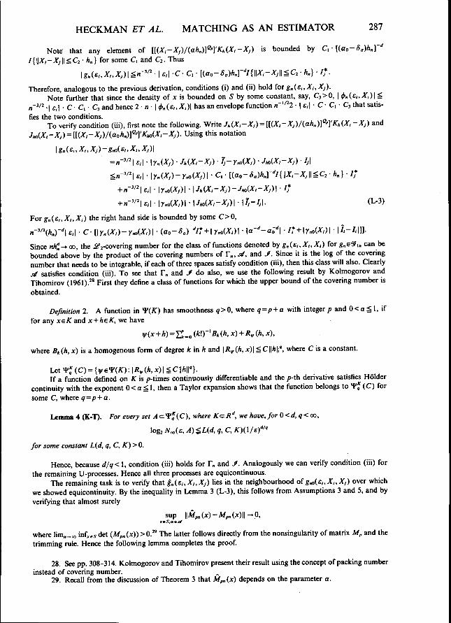
HECKMAN ET AL. MATCHING AS AN ESTIMATOR 287
Note that any element of [[{X,-XJ)/(ah„)\°'\'KH{X,-X)) is bounded by C^•[{ao-S„)h„\-•'l{\\X,-Xj\\<.C2-h^} for some C, and Cj.Thus
^-\ e,\ CQ- Hao-Sa)h„]-'I{\\X,-XJ\\^C2h„} • if.
Therefore, analogous to the previous derivation, conditions (i) and (ii) hold for gn{Si,Xi,Xj).Note further that since the density of x is bounded on 5 by some constant, say, Ci>Q,\4>n(et,X,)\i.
n'^''^-\e,\ • C- Ci- Cj and hence 2 • n • | (^„(e,,X)| has an envelope function w'' ^2 • | e,| • C- C^- Cj that satis-fies the two conditions.
To verify condition (iii), first note the following. Write Ji,(X,-Xj)-^[[(X,-Xj)/{aK)Y'];KH{X,-Xj) andXj) = [[(X-Xj)/(aoK)f'^K^(Xi-Xj). Using this notation
£,| • \r^(Xj) • MX-Xj) • Ij
E>\ • \y„(XJ)-Y.o(XJ)\ • C, • l(ao-Sa)h„]-''I{\\X-XJ\\SC2•h„} • If
^\ e,| • \rno(Xj)\ • \MX!-Xj)-JUX,-Xj)\ • If
Xj)\ -iTj-Ijl. (L-3)
For g„{e,,X|,X|) the right hand side is bounded by some O O ,
Since nA^->oo, the if2-covering number for the class of functions denoted by g,(ei,Xi,X,) for^.eS?], can bebounded above by the product of the covering numbers of F,, si, and J. Since it is the log of the coveringnumber that needs to be integrable, if each of three spaces satisfy condition (iii), then this class will also. Cleariy.s^ satisfies condition (iii). To see that F, and J do also, we use the following result by Kolmogorov andTihomirov (1961)." First they define a class of functions for which the upper bound of the covering number isobtained.
Definition 2. A function in'ViK) has smoothness q>Q, where q=p + a with integer p and 0 < a g 1, iffor any xeK and x + heK, we have
/!, X),
where Bt(h, x) is a homogenous form of degree kinh and \R^(.h, x)\^C\\h\\'', where C is a constant.
Let I f (C) { v ( ) | ^ ( , ) | g | | r }If a function defined on K is p-times continuously differentiable and the p-th derivative satisfies Holder
continuity with the exponent 0< a g 1, then a Taylor expansion shows that the function belongs to f* (C) forsome C, where q=p + a.
Lemma 4 (K-T). For every set Ac:^'^(C), where KczR'', wehave,forO<d,q<co,
Iog2 N^(e, A)^L(d, q, C, K)(\/e)'"''
for some constant L(d, q,C,K)>0.
Hence, because d/q<\, condition (iii) holds for F, and J. Analogously we can verify condition (iii) forthe remaining U-processes. Hence all three processes are equicontinuous.
The remaining task is to verify that §„{£,,Xi,Xj) lies in the neighbourhood of gM(ei,Xi,Xj) over whichwe showed equicontinuity. By the inequality in Lemma 3 (L-3), this follows from Assumptions 3 and 5, and byverifying that almost surely
sup \\M,„(x)-M,„(x)\\->q,xeS.aej^
where limn^« inf^^sdet (M,,(x))>0." The latter follows directly from the nonsingularity of matrix Af, and thetrimming rule. Hence the following lemma completes the proof.
28. See pp. 308-314. Kolmogorov and Tihomirov present their result using the concept of packing numberinstead of covering number.
29. Recall from the discussion of Theorem 3 that M,»(x) depends on the parameter a.
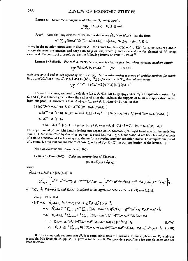
288 REVIEW OF ECONOMIC STUDIES
Lemma 5. Under the assumptions of Theorem 3, almost surely,
sup \\M,„^x)-M,„(x)\\-^O.xeS.aej/
Proof Note that any element of the matrix difference Mp„ (x) - Mp„ (x) has the form
where in the notation introduced in Section A.I the kernel function G(s) = • ^K(s) for some vectors q and rwhose elements are integers and they sum to p or less, where q and r depend on the element of M beingexamined. To construct a proof, we use the following lemma of Pollard (1984).^"
Lemma 6 (Pollard). For each n, tet „ be a separable class of functions whose covering numbers satisfy
supN,(e,&>,'i>„)^Ae''*' for 0<e<\
with constants A and W not depending on n. Let {^„} be a non-increasing sequence of positive numbers for whichlim,^» nC,£,l/\ogn = co. / / | vl g 1 and (E{v'} f'^'^l^^for each y/ in "¥„, then, almost surely.
To use this lemma, we need to calculate N,(e, 9, "V,). Let C, Ssup,e« G(s), Cj is a Lipschitz constant forG, and Cj is a number greater than the radius of a set that includes the support of G. In our application, recallfrom our proof of Theorem 3 that .a = [oo - 5 , , oo + 5.1, where 0 < S. < Oo so that
The upper bound of the right hand side does not depend on 3». Moreover, the right hand side can be made lessthan E • C for some C> 0 by choosing I a i - Oj | g e and | xo, - Xo21 g e. Since S and .aT are both bounded subsetsof a finite dimensional Euclidean space, the uniform covering number condition holds. To complete the proofof Lemma 5, note that we are free to choose ^, = 1 and f „ = C • Af in our application of the lemma. ||
Next we examine the second term (B-3).
Lemma 7 (Term (B-3)). Under the assumptions of Theorem 3
where
"~' ^Z"_i R2(X,) = 0p(\), and Ri^Xo) is defined as the difference between Term (B-3) and b„{xo).
Proof. Note that
(B-3) = c, • lM,Axo)V'n-'H'X',ixo)Wixo)J^f(xo)^*{xo) • I
= e, • [M,„(x„)]- I f . , , , « - i ; . , ll(X,-xo)/(ah„)]<^']'^X,-xo)°'•W^\xo)K,(X,-xo) • /„
= e, • [M,„(xo)]" I f . , , , «-' i ; . , mX,-Xo)/(ah„)]°']'iX,-Xo)'''^'K,(X,-Xo)
- E {l[(X,-Xo)/(ah„)f']'(X^-Xo)'^">K,{X,-Xo)\xo}W'\xo) • I (L-7A)
+ e, • [M^Axo)]-' I f . , , , mliX,-xo)/(ah„)f']'{X,-Xo)°"'K,iX,-Xo)\x„}m'^\xo) • /„. (L-7B)
30. His lemma only requires that .^n is a permissible class of functions. In our applications ^„ is alwaysseparable. His Example 38, pp. 35-36, gives a similar result. We provide a proof here for completeness and forlater reference.
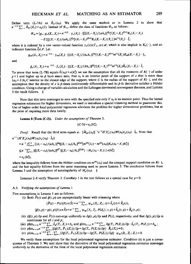
HECKMAN ET AL. MATCHING AS AN ESTIMATOR 289
Define term (L-7A) as Ri\{xo). We apply the same method as in Lemma 2 to show thatn'"^ Z"_i 21 (X) = Op(l). Instead of 'S^„, define the class of functions ^ i , as follows:
where it is indexed by a row vector-valued function •f„(x)eT„, ae.s^, which is also implicit in Ki,(), and anindicator function ijSJ. Let
j X,-XJ) • Ij,
and
To prove that term (L-7B) equals b(xo) + o{hi) we use the assumption that all the moments of Ar(-) of orderp +1 and higher up to p have mean zero, that Xo is an interior point of the support of x that is more than(ao + 5 )/!„ C interior to the closest edge of the support, where C is the radius of the support of Ar( •), and theassumption that the density of x is ^-times continuously differentiable and its p-th derivative satisfies a Holdercondition. Using a change of variable calculation and the Lebesgue dominated convergence theorem, and Lemma5 the result follows. ||
Note that this term converges to zero with the specified rate only if xo is an interior point. Thus for kernelregression estimators for higher dimensions, we need to introduce a special trimming method to guarantee this.Use of higher order local polynomial regression alleviates the problem for higher dimensional problems, but atthe price of requiring more data locally.
Lemma 8 (Term (C-3)). Under the assumptions of Theorem 3,
(C-3) = o,(/.j).
Proof. Recall that the third term equals e, • [Mpn(xo)]'''n''H'X'p(xo)lVixo)rp(xo) • h. Note that
W(xo)rf{xo)Io\\
"-1 [(.X-Xo)/(ah„)]^'1{X,-xo)/h„f'^\m'f\x,) -m'^\xo)]K,(xo-X>)/ij ||
where the inequality follows from the Holder condition on m' '(xo) and the compact support condition on K( •),and the last equality follows from the same reasoning used to prove Lemma 5. The conclusion follows fromLemma 5 and the assumption of nonsingularity of Mp(xo). ||
Lemmas 2-8 verify Theorem 3. Corollary 1 in the text follows as a special case for /? = 0.
A.3. Verifying the assumptions of Lemma 1
Five assumptions in Lemma 1 are as follows:(i) Both P(z) and g(t, p) are asymptotically linear with trimming where
lg{t,p)-g(t,p)]I(xeS) = n-' i ; . , y/„,^YJ, Tj, P{Zj);
(ii) dg(t,p)/dp and P{z) converge uniformly to dg{t,p)/dp and P{z), respectively, and that dg(l,p)/dp iscontinuous for all ( and p;
(iii) p\im„^^n-"^•Z';.,b,(.Tl,XJ) = b, and plim„_„«-'^='S;., dg(T,, P(Z,))/8p b,{T,, P(Z<)) = b,^\(iv) plim„^„«-•/^S;., [di(T,,Pr,(Z,))/Sp-dg(T,,P(Z,))/dp]-R,(Z,) = (i-(V) plim_««-'^^E;-, E ; . , [dg(T,,Pr,(Z,))/8p-dg(T,,P(Z,))/8p] • v'»,(D;, Z^; Z,) = 0.
We verify these assumptions for the local polynomial regression estimator. Condition (i) is just a conse-quence of Theorem 3. We next show that the derivative of the local polynomial regression estimator convergesuniformly to the derivative of the limit of the local polynomial regression estimator.

290 REVIEW OF ECONOMIC STUDIES
Theorem 4. If Assumptions 1-4, and 8 hold, then dg(t,p)/dp is uniformly consistent for dg{t,p)/dp.
Proof For convenience we drop the subscripts p, p, and the argument Xo of X,, (xo), Pp (xo), P* (xo), and^(xo) here so thatX=Xp(xo), P = Pp(xo), P* = P*{xo), and_ W= ^(xo). Also denote the derivative with respectto the first argument of xo by V. Note that X'fVY=X'lVXp. Hence by the chain rule.
Since
{^(X-W)-lV(X'fVX)](X']VX)-'X'W}xp*
we obtain
Note that for.sgl.
= [((A:-XO)<" " ' )„+. .- .„ . , - , , 0 , . . . , 0],
where the second equality follows from our convention on the order of the elements.Thus
VX=-{0 1 0 . . . 0 (;t-xo)e"> 0 . . . 0 . . . (x-xo)^"-" 0 . . . 0).
Note that each column of VX is either a column of X or the column with all elements being 0. Hence thereexists a matrix J such that VX=-XJ, where 7 is a matrix that selects appropriate column of A" or the zerocolumn. Without being more specific about the exact form of J we can see that-(X'fVXy'(X'fVVX)P* = Jp*, and also that
Next, to simplify the last expression, we use some specific properties of matrix J. The key properties of J weuse are that all elements of the first column are 0 and that the first element of the second column of 7 is I. Thatis, the first column of AJ is always the 0-vector, regardless of A and the second column of AJ is the first columnof A. Since the first column is chosen by J exactly once, the preceding observations also imply that the first rowof 7 is ej, where e2 = (0, 1,0,. . . , 0) if p^ 1 and 0, if p = 0. Therefore

HECKMAN ET AL. MATCHING AS AN ESTIMATOR 291
where ei • JP* = Vm(x). That the remaining two terms converge uniformly to zero can be shown analogously asin Lemma S. ||
Condition (iii) of Lemma 1 clearly holds under an i.i.d. assumption given the bias function defined inTheorem 3. In order to verify condition (iv) of the lemma recall the definition of the residual terms and use thesame equicontinuity argument as in the proof of Theorem 3.
Finally condition (v) can be verified by invoking the equicontinuity lemma. This is where the additionalsmoothness condition is required.
Armed with these results, we finally turn to the proof of key Theorem 2.
A.3. Proof of Theorem 2
Note first that, writing I,=I(X,eS),
We first consider the numerator and then tum to the denominator of the expression. Note that the numeratorof the right-hand side of (T-1) is the sum of three terms (TR-l)-(TR-3): writing g, (x) = E5(y,|Z)= LA"=x).
Terms (TR-1) and (TR-2) are analogous to terms we examined in Theorem 1. Term (TR-3) is the additionalterm that arises from estimating g{x). However, the first two terms from Theorem 1 have to be modified toallow for the trimming function introduced to control the impact of the estimation error of g(x).
Central limit theorems do not apply directly to the sums in (TR-1) and (TR-2) because the trimmingfunction depends on all data and this creates correlation across all i. Instead, writing I, = I(XieS), we show thatthese terms can be written as
and
respectively. One can use the equicontinuity lemma and our assumption of p-nice trimming to show the resultfor term (TR-1). The same method does not apply for term (TR-2), however. This is because when we take anindicator function 7/ from J, where / ,#/, , then
It is necessary to recenter this expression to adjust for the bias that arises from using 7,.In order to achieve this we observe that, writing As(A',) = [gi(A'i)-g(A',)]-Es(yi- yol-D=l),
where d(A',) = |/(A',)-/(A',)|, ^-(.s) = 1 i f -1 g.s<0 and 0 otherwise, and ^+(.s)= 1 if Ogj< 1 and 0 otherwise.Since/(X,) = (iVoa»)"''E^^, KiXXi-Xi)lan), the latter two terms can be expressed as double sums. We thenapply an equicontinuity argument to the expressions
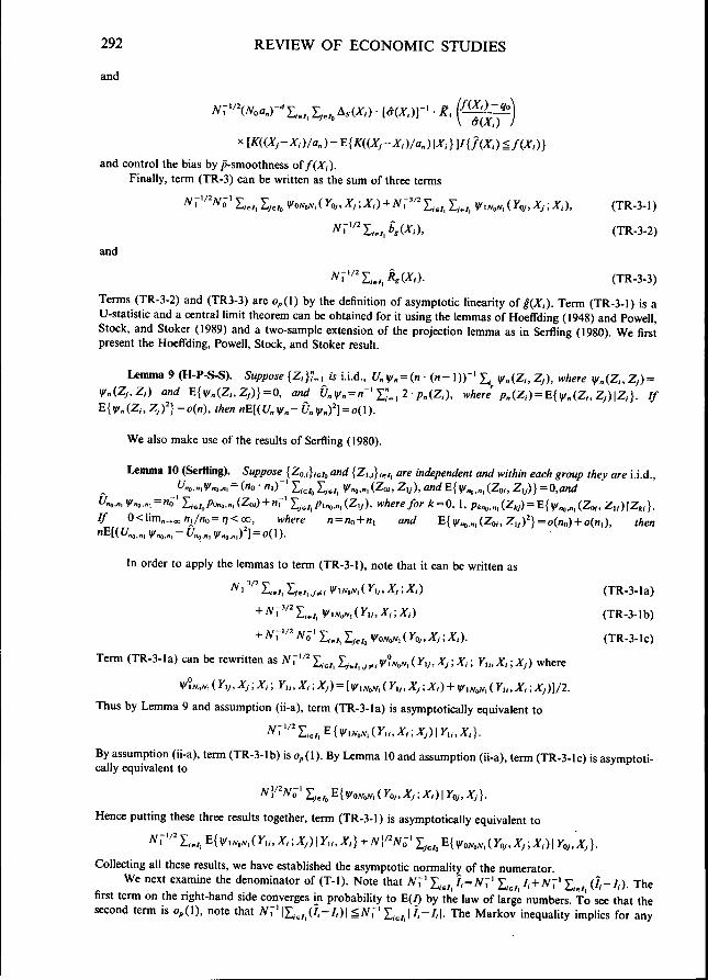
292 REVIEW OF ECONOMIC STUDIES
and
and control the bias by ^-smoothness of/(A",).Finally, term (TR-3) can be written as the sum of three terms
and
^,^ £. , V<^MYoj,Xj;X,), (TR-3-1)
(TR-3-2)
(TR-3-3)
Terms (TR-3-2) and (TR3-3) are 0,(1) by the definition of asymptotic linearity of (;ir,). Term (TR-3-1) is aU-statistic and a central limit theorem can be obtained for it using the lemmas of Hoeffding (1948) and Powell,Stock, and Stoker (1989) and a two-sample extension of the projection lemma as in Serfling (1980). We firstpresent the Hoeffding, Powell, Stock, and Stoker result.
Lemma 9 (H-P^S). Suppose {Z,}?., is i.i.d., U„y/„=in • ( n - 1))-' J,. V»(Z,, Z,), where ^,„{Z,, Zj) =
Vn{Zj,Z,) and V.{v^(Z,,Zj)}=Q, and &„ V-. = ' ' " ' I ^ . . , 2 •;7,(Z,), H-Zie/-/ ;,,(Z,) = E{v,,(Z,, Z,)|Z,}. / /
^{^l^„(Zi,ZJf}=o(n), then /IE[(t/„ v , - [ / „ ,/'„)'] = o(l).
We also make use of the results of Serfling (1980).
Lemma 10 (Serfling). Suppose {Zaj},,,^ and {Z,,,},^,, are independent and within each group they are i.i.d.,Un,.., Vn,.n, = ("o ' «,)^' !,„„ I, , , , w^.., (Zoi, Z,j), and E{ ^ ^ , „ , (Zoi, Z,j)} = O,and
t4o.», W.o.m = no ' I,,,,/'o^o.,, (Zo,) -I- nr' I,.,,, p,^.^, (Z,j), where for k = Q,\, p,^,„^ (Z,j) = E{ ^>^,^^ (Zo,, Z,,) |Z*,}./ / 0<lim»^» «,/«„=;;< 00, where « = «„ + /,, and E{v^^,»,(Zo,, Z,^)^} =o(no) + o(n,), then
E[(f/ U )'] (l)
In order to apply the lemmas to term (TR-3-1), note that it can be written as
^ r ' ^ ' I,^,, I,.^,, j ^ , ViATjAT, (Y,j, XJ ; X,) (TR-3-la)
+ A^r'^'Z,e,, Vi«.Ar,(r,,,X,;.y,) (TR-3-lb)
+ N^"^ No' E,,,, Y.J,,, VowoAT,(Ko,,XJ;.V,). (TR-3-lc)
Term (TR-3-la) can be rewritten as Afr'^' I , , , , E,.^,, ^^. v?;vo«, (Y,j, Xj; , ; Y,,, X,; A ) where
Wif^o^, ( J'ly, A-y; X,; X,,, A-,; A ,) = [y,,^^,,, (K,,, A ,; X ) + VI VOA-, (X,,, A",; Ay)]/2.
Thus by Lemma 9 and assumption (ii-a), term (TR-3-la) is asymptotically equivalent to
A^r'-" I , , , , E {v/,;v<,/v, (Yu,X<; XJ)I y,,, AT,}.
By assumption (ii-a), term (TR-3-Ib) is o,( l) . By Lemma 10 and assumption (ii-a), term (TR-3-lc) is asymptoti-cally equivalent to
j ^ A-, ( YOJ, XJ ; X,)\ YOJ, XJ}.
Hence putting these three results together, term (TR-3-1) is asymptotically equivalent to
Collecting all these results, we have established the asymptotic normality of the numerator.We next examine the denominator of (T-1). Note that N^' E, , ii=N'[' E_ , I, + NT' £.^, ( / , - / , ) . The
first term on the right-hand side converges in probability to E(/) by the law of large numbers. To see that thesecond term is o,(l), note that Afr ' l l , , , ,(7,-/ ,) | gAT' I , , , , | / , - / , | . The Markov inequality implies for any

HECKMAN ET AL. MATCHING AS AN ESTIMATOR 293
e>0, Pr {AT' X,^, |7i-/, |>£}gE{|/,-/ ,!}/£. Hence assumption (ii-d) implies that the second term iso,(l).This result, in conjunction with our result for the denominator, proves Theorem 2. ||
Acknowledgements. The work reported here is a distant outgrowth of numerous conversations withRicardo Barros, Bo Honore, and Richard Robb. We thank Manuel Arellano and three referees for helpfulcomments. An eariier version of this paper "Matching As An Evaluation Estimator: Theory and Evidence onIts Performance applied to the JTPA Program, Part L Theory and Methods" was presented at the Review ofEconomic Studies conference on evaluation research in Madrid in September, 1993. This paper was also presentedby Heckman in his Harris Lectures at Harvard, November, 1995, at the Latin American Econometric Societymeeting in Caracas, Venezuela, August, 1994; at the Rand Corporation, U.C. Irvine, U.S.C., U.C. Riverside,and U.C. San Diego September, 1994; at Princeton, October, 1994; at UCL London, November, 1994 andNovember, 1996, and at Texas, Austin, March, 1996 and at the Econometric Society meetings in San Francisco,January, 1996.
REFERENCESARCONES, M. A. and G I N 6 , E. (1993), "Limit Theorems for U-processes", Annals of Probability, 21, 1494-
1542.BARNOW, B., CAIN, G. and GOLDBERGER, A. (1980), "Issues in the Analysis of Selectivity Bias," m E.
Stromsdorfer and G. Farkas (eds.). Evaluation Studies Review Annual, Volume 5 (San Francisco: Sage).BARROS, R. (1986), "Nonparametric Estimation of Causal Effects in Observational Studies" (University of
Chicago, mimeo).COCHRANE, W. G. and RUBIN, D. B. (1973), "Controlling Bias In Observational Studies", Sankyha, 35,
417-446.DAWID, A. P. (1979), "Conditional Independence in Statistical Theory", Journal of The Royal Statistical
Society Series B, 41, 1-31.FAN, J. (1993), "Local Linear Regression Smoothers and Their Minimax Efficiencies", The Annals of Statistics,
21, 196-216.FAN, J., HARDLE, W. and MAMMEN, E. (1996), "Direct Estimation of Low Dimensional Components m
Additive Models" (Working paper).HAHN, J. (1996), "On the Role of the Propensity Score in the Efficient Semiparametric Estimation of Average
Treatment Effects" (unpublished manuscript. University of Pennsylvania).HECKMAN, J. (1974), "Shadow Prices, Market Wages, and Labor Supply", Econometrica, 42, 679-694.HECKMAN, J. (1990), "Varieties of Selection Bias", American Economic Review, 80, 313-318.HECKMAN, J. (1997), "Instrumental Variables: A Study of the Implicit Assumptions Underlying One Widely
Used Estimator for Program Evaluations", Journal of Human Resources, 32, 441-462.HECKMAN, J., ICHIMURA, H., SMITH, J. and TODD, P. (1996a), "Nonparametric Characterization of
Selection Bias Using Experimental Data, Part II: Econometric Theory and Monte Cario Evidence"(Unpublished manuscript. University of Chicago).
HECKMAN, J., ICHIMURA, H., SMITH, J. and TODD, P. (19966), "Sources of Selection Bias in EvaluatingPrograms: An Interpretation of Conventional Measures and Evidence on the Effectiveness of MatchingAs A Program Evaluation Method", Proceedings of The National Academy of Sciences, 93, 13416-13420.
HECKMAN, J., ICHIMURA, H., SMITH, J. and TODD, P. (1998), "Characterizing Selection Bias UsingExperimental Data", Econometrica (forthcoming).
HECKMAN, J., ICHIMURA, H. and TODD, P. (1997), "Matching As An Econometric Evaluation Estimator:Evidence from Evaluating a Job Training Program", Review of Economic Studies, 64, 605-654.
HECKMAN, J. and ROBB, R. (1985), "Altemative Methods For Evaluating The Impact of Interventions", inJ. Heckman and B. Singer (eds.). Longitudinal Analysis of Labor Market Data (Cambridge: CambridgeUniversity Press).
HECKMAN, J. and ROBB, R. (1986), "Altemative Method For Solving the Problem of Selection Bias inEvaluating The Impact of Treatments on Outcomes," in H. Wainer (ed.). Drawing Inferences from Self-Selected Samples (New York: Springer-Veriag).
HECKMAN, J. and SMITH, J. (1998), "Evaluating The Welfare State", Frisch Centenary, Econometric Mono-graph Series (Cambridge: Cambridge University Press), forthcoming.
HECKMAN, J., SMITH, J. and CLEMENTS, N. (1997), "Making the Most Out of Social Experiments:Reducing the Intrinsic Uncertainty in Evidence From Randomized Trials With An Application to theNational JTPA Experiment", Review of Economic Studies, 64, 487-535.
ICHIMURA, H. (1993), "Semiparametric Least Squares (SLS) and Weighted SLS Estimation of Single IndexModels", Journal of Econometrics, 58, 71-120.
ICHIMURA, H. (1995), "Asymptotic Distribution of Nonparametric and Semiparametric Estimators withData-Dependent Smoothing Parameters" (Unpublished manuscript. University of Chicago).
KOLMOGOROV, A. N. and TIHOMIROV, V. M. (1961), "e-Entropy and £-Capacity of Sets in FunctionalSpaces", American Mathematical Society Translations, series 2, 17, 277-364.
294 REVIEW OF ECONOMIC STUDIES
LINTON, O. and NIELSON, J. P. (1995), "A Kernel Method of Estimating Structural Nonparametric Regres-sion Based on Marginal Integration", Biometrika, 82, 93-100.
NOLAN, D. and POLLARD, D. (1987), "U-processes: Rates of Convergence", Annal of Statistics, 15, 405-414.
NEWEY, W. K. and McFADDEN, D. L. (1994), "Large Sample Estimation And Hypothesis Testing", in R.F. Engle and D. L. McFadden (eds.). Handbook of Econometrics. Vol. IV. (Amsterdam: Elsevier).
MASRY, E. (1995), "Multivariate Local Polynomial Regression for Time Series" (Unpublished manuscript).POLLARD, D. (1990), Empirical Processes: Theory and Applications (Hayward: IMS).POWELL, J. L., STOCK, J. H. and STOKER, I. M. (1989), "Semiparametric Estimation of Index Coefficients",
Econometrica, 57, 1403-1430.ROSENBAUM, P. and RUBIN, D. B. (1983), "The Central Role of the Propensity Score in Observational
Studies for Causal Effects", Biometrika, 70, 41-55.RUPPERT, D. and WAND, M. P. (1994), "Multivariate Locally Weighted Least Squares Regression" The
Annals of Statistics, 22, 1346-1370.SERFLING, R. J. (1980), Approximation Theorems of Mathematical Statistics (New York: Wiley).SHERMAN, R. P. (1994), "Maximal Inequalities for Degenerate U-processes with Applications to Optimization
Estimators", Annal of Statistics, 11, 439-459.STONE, C. (1982), "Optimal Global Rates of Convergence For Nonparametric Regression", Annals of Statistics
10, 1040-1053.TJOSTHEIM, D. and AUESTAD, B. H. (1994), "Nonparametric Identification of Nonlinear Time Series:
Projections", Journal of the American Statistical Association, 89, 1398-1409.WESTAT, INC. (1980), "Net Impact Report No. 1, Impact on 1977 Eamings of New FY 1976 CETA Enrollees
in Selected Program Activities" (Rockville, Maryland, Westat Inc.).WESTAT, INC. (1982), "CLMS Follow up Report No. 7 (18 Months After Entry), Postprogram Experiences
and Pre/Post Comparisons For Terminees Who Entered CETA During July 1976 Through September1977" (Rockville, Maryland, Westat Inc.).
WESTAT, INC. (1984), "Summary of Net Impact Results" (Rockville, Maryland, Westat Inc.).
