econ 839 econometrics iib sept 12, 2011 - sfu.cahaiyunc/notes/econ 839 notes.pdf · econ 839...

Econ 839 Econometrics IIB Sept 12, 2011

of 54

Introduction

Chris, WMC 3639, [email protected]

Textbook and organization of the course

Part I: read it (for fun)

Part II: core methods

Ch.4. – prerequisite

Ch.5. – review (maximum likelihood)

Ch.6. – review (GMM)

Ch.9. – depends on you (semi-parametric)

Part III: bootstrap (probably skip)

Part IV: important!! (except 17, 18, 19)

Part V: panel data, 21, 22, maybe 23

Part VI: Ch.25 (program evaluation)

mailto:[email protected]


of 54

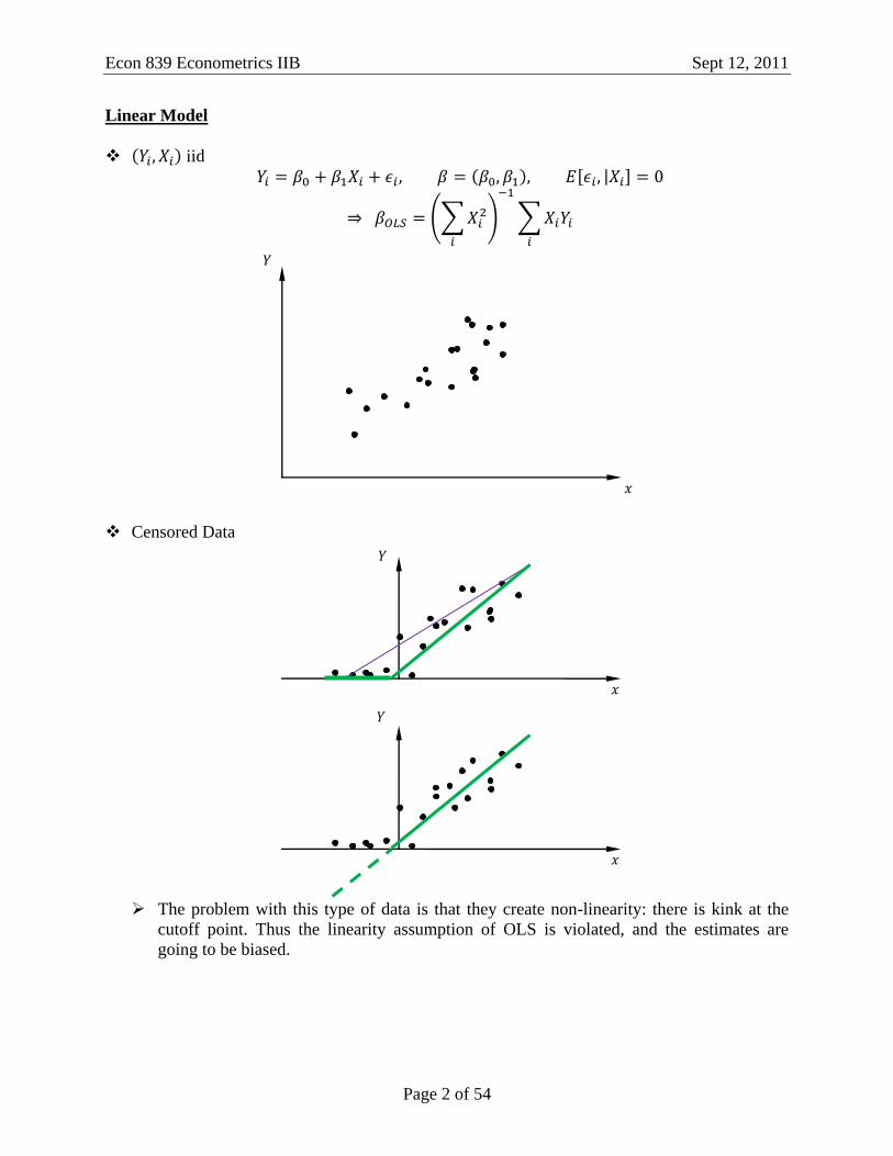
Linear Model

iid

Censored Data

The problem with this type of data is that they create non-linearity: there is kink at the

cutoff point. Thus the linearity assumption of OLS is violated, and the estimates are

going to be biased.


of 54

OLS – Cens – Binary choice –

Multinomial –

Program evaluation – how well does a program (e.g. education voucher) work?

But selection issue may bias the estimated result.

Penal Data

Standard linear model:

Panel data model:


of 54

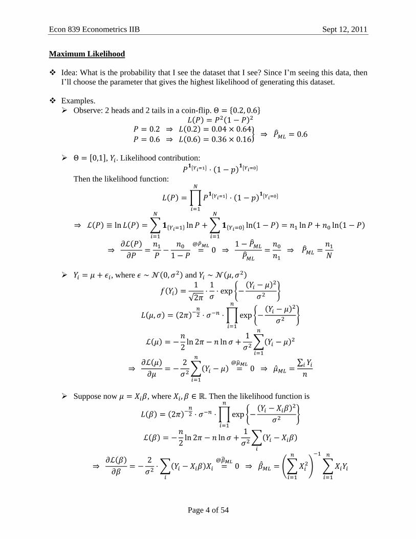
Maximum Likelihood

Idea: What is the probability that I see the dataset that I see? Since I’m seeing this data, then

I’ll choose the parameter that gives the highest likelihood of generating this dataset.

Examples.

Observe: 2 heads and 2 tails in a coin-flip.

, . Likelihood contribution:

Then the likelihood function:

, where and

Suppose now , where . Then the likelihood function is


of 54

Properties of Maximum Likelihood Estimator

Cameron & Trivedi, Chapter 5

Background Appendix A

CH. 5: 5.1, 5.2, 5.3, 5.6

More. Newey, McFadden, Handbook of Econometrics IV, Chpt 36

iid observations,

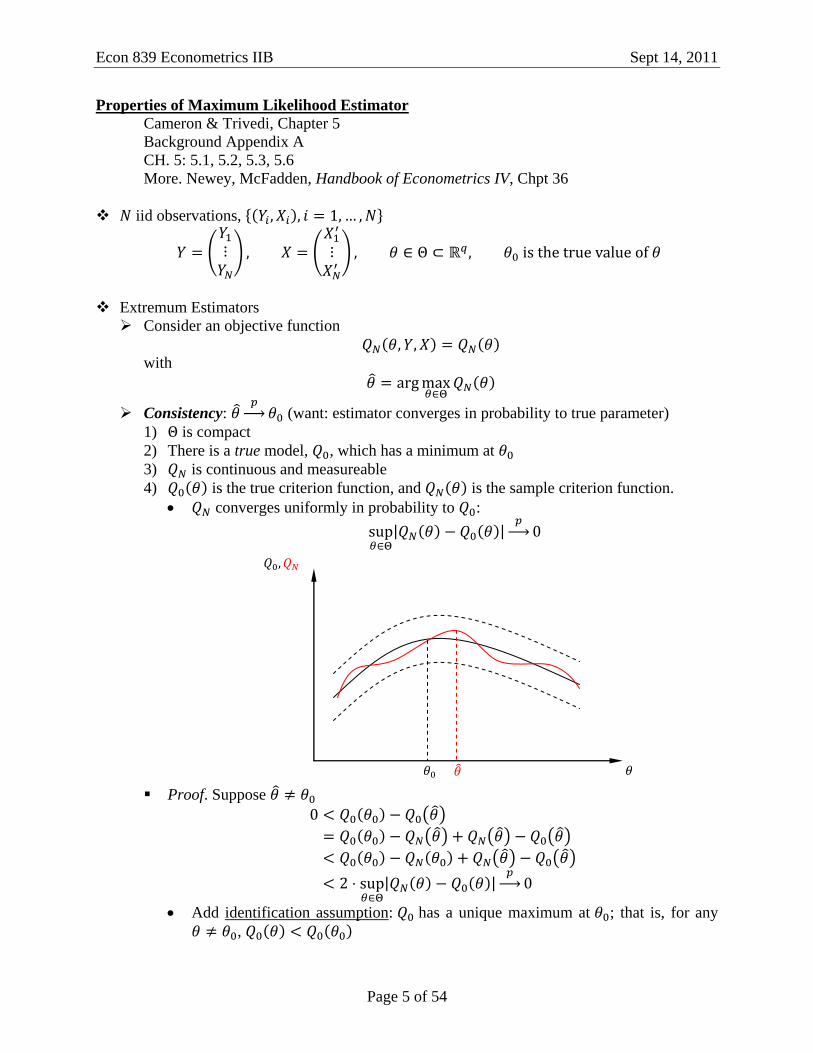
Extremum Estimators

Consider an objective function

with

Consistency: (want: estimator converges in probability to true parameter)

1) is compact

2) There is a true model, , which has a minimum at

3) is continuous and measureable

4) is the true criterion function, and is the sample criterion function.

converges uniformly in probability to :

Proof. Suppose

Add identification assumption: has a unique maximum at ; that is, for any

,


of 54

Asymptotic Normality.

with

Use a Taylor expansion:

Maximum Likelihood Estimator (MLE) is an extremum estimator

LLN

Evaluate the criterion function at and


of 54

Binary Choice

C & T Chapter 14, study parts 1, 2, 3, 4; read 8

Introduction

Set up Model

Estimation

Identification

Marginal effects, interpretation of parameters

Properties of estimator

Intro: choice of fishing mode

and relative price of boat v.s. pier

Why not OLS?

but →

this leads to interpretational issues

→ this leads to heteroscedasticity

Interpret as the “attractiveness of boat fishing to person

Let .


of 54

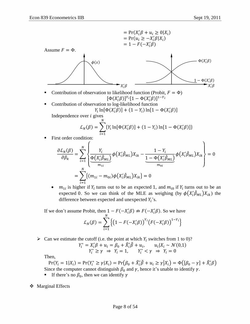
Assume .

Contribution of observation to likelihood function (Probit, )

Contribution of observation to log-likelihood function

Independence over gives

First order condition:

is higher if turns out to be an expected , and if turns out to be an

expected . So we can think of the MLE as weighing (by ) the

difference between expected and unexpected ’s.

If we don’t assume Probit, then

. So we have

Can we estimate the cutoff (i.e. the point at which switches from 1 to 0)?

Then,

Since the computer cannot distinguish and , hence it’s unable to identify .

If there’s no , then we can identify

Marginal Effects


of 54

Linear model: with

In the linear case, the marginal effect is always flat.

Binary choice:

In the binary choice case…

the sign of determines the sign of marginal effect

ME depends on

Logit – choice of the distribution of

Recall the model we’ve been working on:

Some calculus:


of 54

Let . Then,

We thus have

Odds ratio (ratio between two probabilities):

Log odds ratio:

If increases by , log odds increase by

Consistency for binary choice

Theorem. 5.1. Under some conditions,

as (where ).

The conditions are

is compact

Just pick

is measurable and continuous for all

Just assume measurability is satisfied. For continuity, in the case of logit

is continuous.

converges uniformly to , and has a unique maximum at

converges pointwise to , since it’s also bounded, uniform convergence is

guaranteed

For the existence of unique global maximum, need to be globally concave

Econ 839 Econometrics IIB September 26, 2011

of 54

Demystifying the Criterion Function

Examples of Criterion Functions

For maximum likelihood:

For OLS:

For non-linear least square with additive error term ( ):

For GMM:


of 54

Multinomial Choice

Cameron & Trivedi, Ch.15: 15.1 – 15.6, 15.8, 15.9 (optional 15.6 and 15.8)

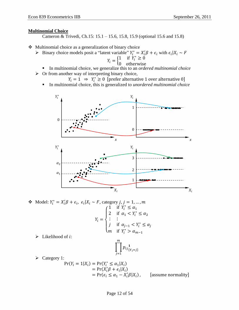
Multinomial choice as a generalization of binary choice

Binary choice models posit a “latent variable”

with

In multinomial choice, we generalize this to an ordered multinomial choice

Or from another way of interpreting binary choice,

In multinomial choice, this is generalized to unordered multinomial choice

Model:

, category ,

Likelihood of :

Category 1:


of 54

Category :

Category : homework.

Suppose . Likelihood contribution of individual

Parameters: , , and let . The log-likelihood is

Interpretation of Model ( ), Linear model: ,

1)

As increases, changes by . But this interpretation is “silly” because we don’t

really observe .

2) , assume and probit,

In this case, the sign of is not informative, because the sign of is undetermined.

Solution:


of 54

If is positive, then the probability of being in a lower category decreases as

goes up marginally.

Unordered Multinomial. Micro-foundation to the binary choice model (aka the Adaptive

Random Utility Model):

Normalize and let , and →

→

Similarly, in the multinomial case, we posit the following:

Assume independent across (IIA), and let the distribution of be “Type 1 EV”:

Guide to 14.3 (Multinomial Logit and Conditional Logit)

For estimation, treat everything as if it is a CL. If it happens to be ML, then construct a

new set of regressors in the following way:

Marginal Effects

Conditional logit

Alternative 1

Alternative 2


of 54


of 54

Unordered Multinomial Choice

alternatives, each associates with utility

Assumption on

1) are mutually independent

2) , Type 1 Extreme Value distribution

Marginal Effects for Conditional Logit

Regressors

Let . Then,

Marginal effects depends on

Marginal effects are larger for intermediate values of

For ,


of 54

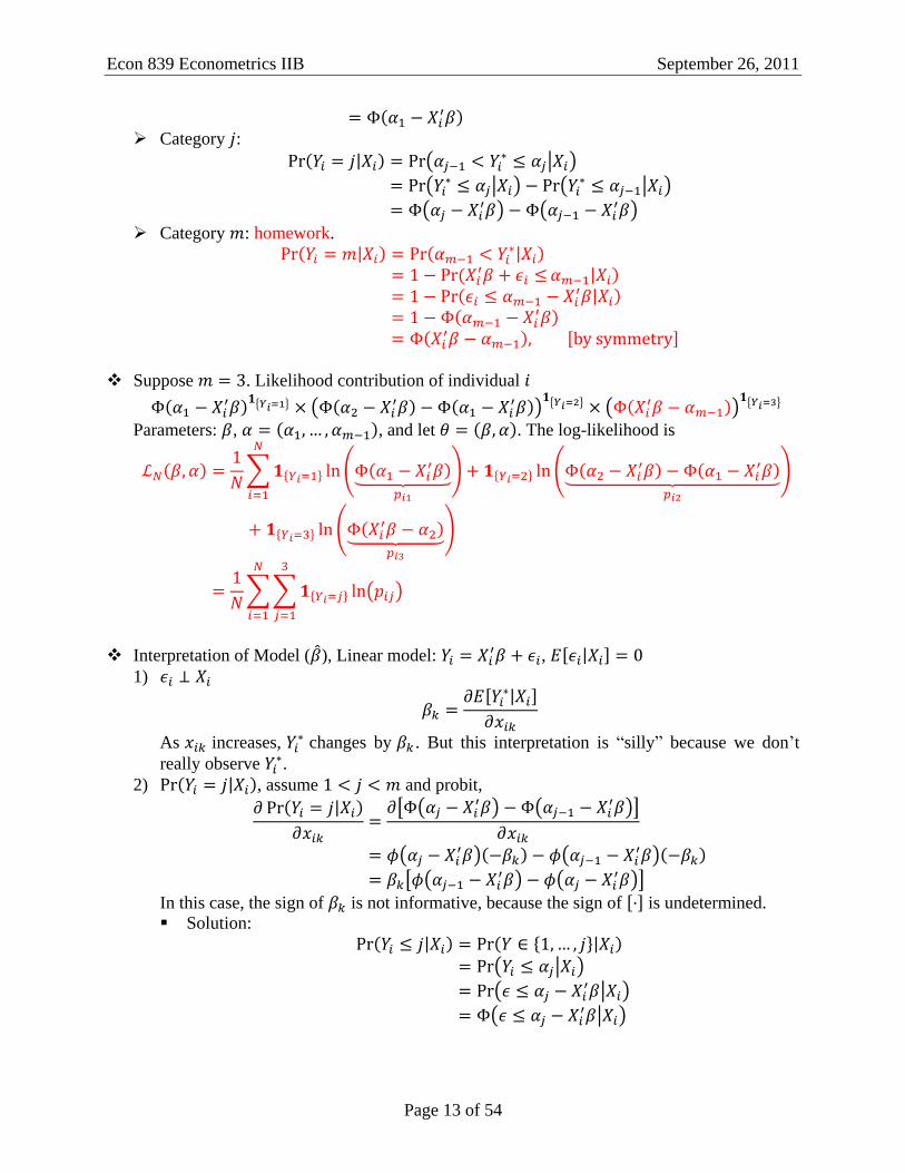
What’s the probability of being in another category?

If increases,

Econ 839 Econometrics IIB October 3, 2011

of 54

Tobit + Selection

Ch. 16.1 – 16.6

Skip 16.2.4, 16.2.5, 16.3.6, 16.6.7 (and don’t worry about LEF)

Plus whatever we do out of 16.10

Censoring and Truncation

Censoring and truncation imply non-linearity in the model.

Usually we start with some conditional mean, and by omitting observations below zero

(truncation or censoring), the regression we get are going to have a higher condition

mean for close to zero.

A latent-variable model

is the observed dependent variable (e.g. # of hours worked)

is unobserved dependent variable (e.g. desired # of hours worked)

is censoring or truncation cutoff

Censoring:

Truncation:

is the conditional pdf of

Censoring: conditional distribution of (observed dependent variable)

Censoring

truncated at


of 54

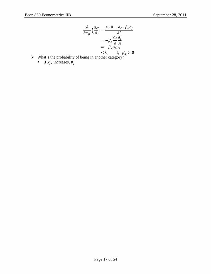
Introduce another variable:

Then,

are iid copies of

Truncation: note the difference between and

Likelihood function:

Tobit

Marginal effects:

For all observations above the cutoff: simply change by

For all below and not close to cutoff: no effect

For all below but close to cutoff: probability that it’ll jump to above cutoff +

Conditional means (suppose )

Truncated mean:

Only look at people who are already working


of 54

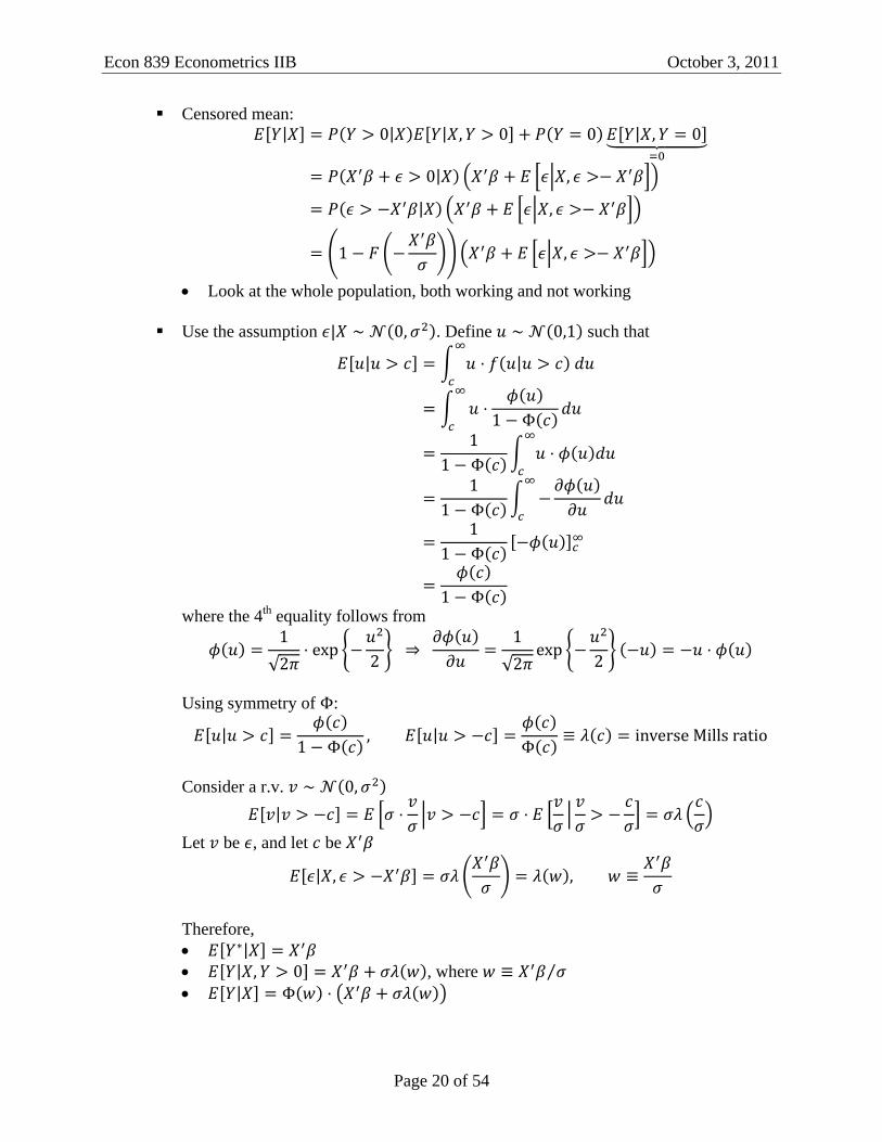
Censored mean:

Look at the whole population, both working and not working

Use the assumption . Define such that

where the 4th

equality follows from

Using symmetry of :

Consider a r.v.

Let be , and let be

Therefore,

, where


of 54

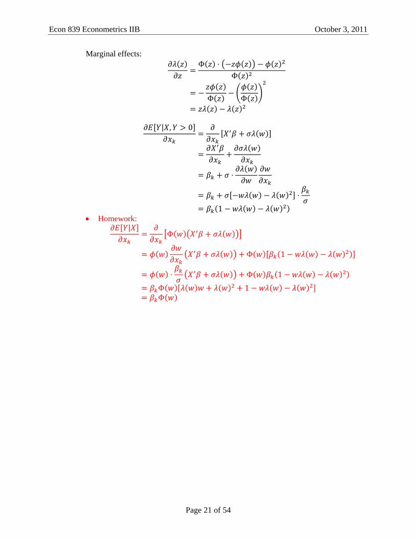
Marginal effects:

Homework:


of 54

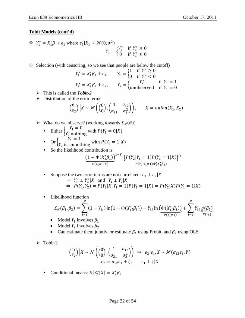
Tobit Models (cont’d)

where

Selection (with censoring, so we see that people are below the cutoff)

This is called the Tobit-2

Distribution of the error terms

What do we observe? (working towards )

Either

with

Or

with

So the likelihood contribution is

Suppose the two error terms are not correlated:

Likelihood function

Model involves

Model involves

Can estimate them jointly, or estimate using Probit, and using OLS

Tobit-2

Conditional means:


of 54

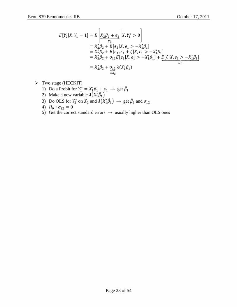
Two stage (HECKIT)

1) Do a Probit for

→ get

2) Make a new variable

3) Do OLS for on and

→ get and

4)

5) Get the correct standard errors → usually higher than OLS ones


of 54

Stata Tricks

Stata commands

-list in 1/10- after the –use- to show observations 1 to 10

-list if price>10- shows observations where price is greater than 10

-list c1-wage in 1/10- shows first 10 observations for variables “c1” to “wage”

-insheet varname1 varname2 ... using dataset.csv- loads dataset and assign

names to each column of data

-infix varname1 1-2 varname2 3-4 ... using dataset.fix- loads fixed format

dataset and assign names to designated columns of data.

In this example, columns 1 and 2 belong to variable 1, 3 and 4 to variable 2, etc.

There are different ways of coding missing data, and Stata treats them as ., .a, .b, etc. If

you want to replace all these missing values use –replace varname = 500 if varname>=.-

MLE in Stata

All we need is just the likelihood function, then we get the estimator and the standard

errors for free

Estimator is the maximand of the likelihood function

Standard errors come from the Jacobian of the likelihood function

OLS: with

Probit: , and


of 54

Midterm Answer

Question 4 (b)

where


of 54

Duration

C&T Ch 17.1 – 17.4, 17.6 – 17.

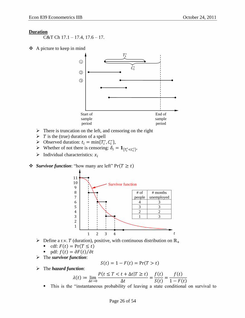
A picture to keep in mind

There is truncation on the left, and censoring on the right

is the (true) duration of a spell

Observed duration:

, Whether of not there is censoring:

,

Individual characteristics:

Survivor function: “how many are left”

Define a r.v. (duration), positive, with continuous distribution on

cdf:

pdf:

The survivor function:

The hazard function:

This is the “instantaneous probability of leaving a state conditional on survival to

Survivor function

# of

people

# months

unemployed

4 3

3 3

2 2

1 3

Start of

sample

period

End of

sample

period

○1

○2

○3


of 54

time .” This function answers the question “What is the probability that a person’s

unemployment spell ends now, given he has been unemployed for periods?”

Cumulative hazard function:

1) Survivor function:

2) Expectation of duration :

Thus, the expectation of duration is the area under the survivor curve.

3) Hazard function:

4) Alternative way of expressing survivor function:

5) Cumulative hazard function:

Thus,


of 54

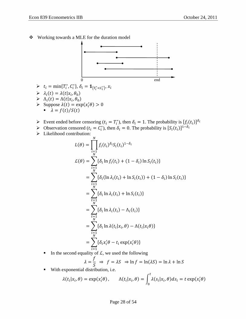
Working towards a MLE for the duration model

,

,

Suppose

Event ended before censoring ( ), then . The probability is

Observation censored ( ), then . The probability is

Likelihood contribution:

In the second equality of , we used the following

With exponential distribution, i.e.

end


of 54

Duration Model (cont’d)

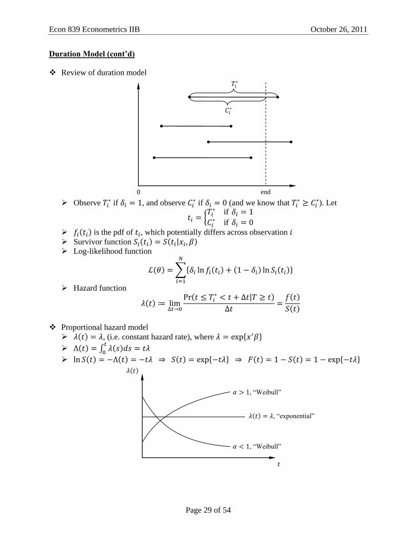
Review of duration model

Observe

if , and observe if (and we know that

). Let

is the pdf of , which potentially differs across observation Survivor function

Log-likelihood function

Hazard function

Proportional hazard model

, (i.e. constant hazard rate), where

, “exponential”

, “Weibull”

, “Weibull”

end


of 54

Suppose the hazard rate is not constant. Then we’d use the Weibull distribution.

Regressors: ,

The shape of the hazard function is determined by (or ), the baseline harzard

function.

If you assume the PH model, then you don’t need to know what is. But

proportionality is restrictive.

Generalized Weibull (which allows for non-monotone hazard functions)

Look at the log of G-Weibull

Hence we can get a U-shape hazard function.

Answer to Leanna’s question

Suppose data is uncensored, i.e. , and is the length of complete spell

Likelihood contribution

There are two random variables:

Suppose is independent of .

Uninformativeness: and are non-overlapping


of 54

Transition (Duration) Data

Data on durations

is the length of completed spell

is censoring time

Observe and , and covariates

Assume model (distribution) for

Either , , , , or will work.

Pick

Collect iid data on

Write down likelihood function [note that we have censoring]

Ignore (the regressors)

Assume are independent (so that are independent). Then .

The log-likelihood is

Note that .

Assume

where and do not overlap (i.e. none of their elements coincide).

We’re interested in . The that maximizes also maximizes

This is the conditional MLE (CMLE): we estimate conditional on that we know

the distribution of .

We’ve shown that


of 54

Popular family of models is the family of Proportional Hazard (PH) models.

PH model (when the hazard function can be written as two components, one depends on

and the other depends on ):

With exponential: , , then the hazard (rate)

is constant at , given the set of regressors . If we change the regressors,

the hazard rate will shift either up or down, but still independent of .

The model is called “proportional” in the sense that

1. can only shift , but not its shape

2. is constant (in the case of exponential distribution)

These two are also what make the model too restrictive

With Weibull, we can make the baseline hazard ( ) go up or down

With generalized Weibull, we can have a U-shaped

But these generalizations still cannot address 1., the shape is still unaffected by the

regressors

Cox PH model.

Keep objection 1. (still a proportional model)

Get rid of 2 completely

is parametric, but is not restricted (we can estimate without

imposing any structure on

But still, even with this level of flexibility, is still a scale factor

Marginal effects (in the case of exponential model )

In general,

Estimation of the PH model.

Think of it as discrete time: (“failure time”) and

Order observations according the length of the durations, from smallest to largest

Risk set: is the set of observation that didn’t “die” yet.

“Death” set: , with

Ties: , i.e. more than one spell ends at

Assume no ties. The probability of the th observation dying at time is


of 54

If we have ties, then

The “likelihood function” is

Choose to maximize

Note that is not in the likelihood function

But we have results showing that is a consistent estimator of this model

We are often not interested in . But how do we estimate if we ever get interested?

ox: hazard free

PH: fully specif

Likelihood:

Think of observation , dies at , and its likelihood contribution is

This leads to a likelihood function

Then, use the knowledge of to back out the ’s by estimating

Econ 839 Econometrics IIB November 2, 2011

of 54

GMM Review

C&T Ch.6.1 – 6.6

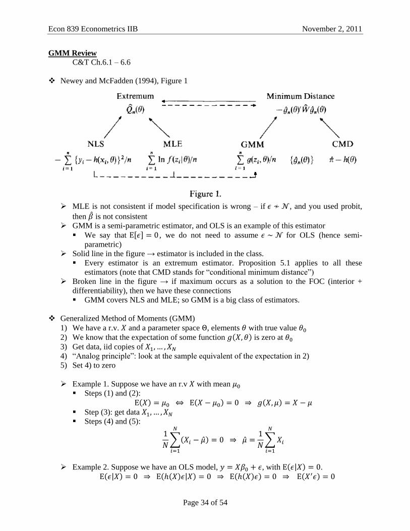
Newey and McFadden (1994), Figure 1

MLE is not consistent if model specification is wrong – if , and you used probit,

then is not consistent

GMM is a semi-parametric estimator, and OLS is an example of this estimator

We say that , we do not need to assume for OLS (hence semi-

parametric)

Solid line in the figure → estimator is included in the class.

Every estimator is an extremum estimator. Proposition 5.1 applies to all these

estimators (note that CMD stands for “conditional minimum distance”)

Broken line in the figure → if maximum occurs as a solution to the FOC (interior +

differentiability), then we have these connections

GMM covers NLS and MLE; so GMM is a big class of estimators.

Generalized Method of Moments (GMM)

1) We have a r.v. and a parameter space , elements with true value

2) We know that the expectation of some function is zero at

3) Get data, iid copies of

4) “Analog principle”: look at the sample equivalent of the expectation in 2)

5) Set 4) to zero

Example 1. Suppose we have an r.v with mean

Steps (1) and (2):

Step (3): get data

Steps (4) and (5):

Example 2. Suppose we have an OLS model, , with .


of 54

Note that , , , , and hence

Steps (1) and (2):

is a random sample of . Hence,

Sample analog

Example 3. , with , and hence

Random sample: . Thus the sample analog:

Example 4. , where and have the same dimension.

However, assume . Then

Note that we’ve assumed in the previous examples.

Function has components, and has components. There are more components

of than parameters.


of 54

GMM (cont’d)

We have , iid data , and the analog principle:

where is and is . But the equality can hold only when .

When , one solution is to introduce a matrix

This leads to a criterion function

Example. with , where , , .

The criterion function is

notations:

Hence the criterion function simplifies to

The derivative

Let

Set

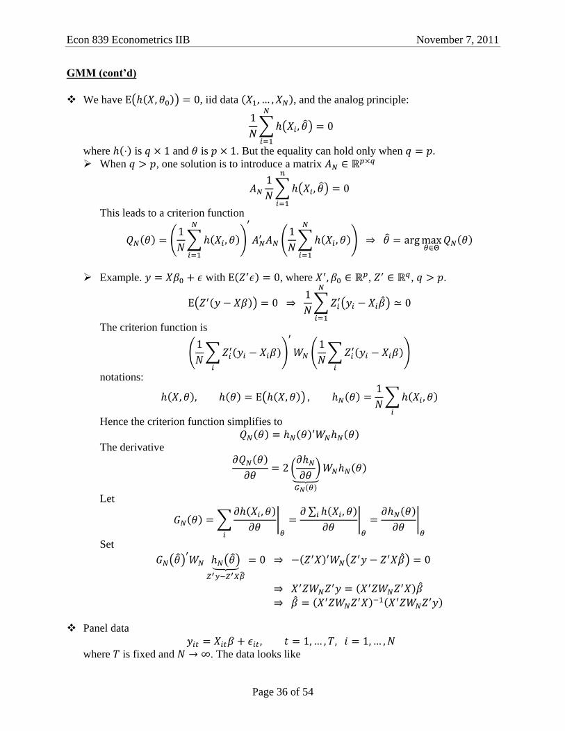
Panel data

where is fixed and . The data looks like


of 54

There are moment conditions

where and each regressor are exogenous, i.e.

.

Another way to impose exogeneity is to have

Here we have moment conditions.

These show the advantage of GMM: you have more moment conditions, depending how

you assume the exogeneity between variables across time, etc., you’ll get even more.


of 54

GMM Theory: Consistency, Asymptotic Normality, and Efficiency

Definition.

where

.

Theorem (Consistency). If

1) are iid

2)

3) Uniform convergence of to . This is satisfied when

a. is continuous in

b.

c. is compact

4)

a positive definite and symmetric matrix

then .

Proof. General steps

(3) gives uniform convergence of to , i.e.

Imply uniform convergence of to ?

Imply pointwise convergence of to ?

Imply ?

Now the proof:

Thus we’ve shown that

We know that

Since ,

This completes the proof.


of 54

Recall the derivative of is

Assume and consistency of . Then,

Apply the Mean value expansion

where

Therefore,

where

Theorem (Asymptotic Normality). If

1) All conditions of the consistency theorem hold

2) , i.e. variance of the moment condition at the true

value is finite

3)

is continuous and uniformly bounded

Note also that

pointwise. So pointwise convergence together with

continuity and uniform boundedness gives uniform convergence of to .

4) has full rank

then .


of 54

GMM Theory (cont’d)

Recall from last time:

Consistency:

Asymptotic normality: , where

Optimal is

To show that is indeed optimal, we show that the expression

is positive definite. Pre- and post-multiply ,

Thus we want to show that is positive definite. is PD if is PD.

is PD if is idempotent, i.e. and .

If is idempotent, then is idempotent.

Notice that is like a projection matrix (let

), , which is

idempotent. Thus we can conclude that

To implement GMM, the traditional way:

Choose

Get

Estimate by Get


of 54

Panel Data

C&T Ch. 21, skip 21.5

Example

Panel data model

usually let and .

Benefits of using Panel data

Simply have more data, more information, allows

Allows us to deal with omitted variable bias, e.g. laziness of people

Get free instrument

Log hourly wage

Log hours

Individual 1

Individual 2

Difference

in individual

effect

Pooled OLS

regression

line


of 54

Panel Data (cont’d)

C&T Ch.21.2.3 will not be lectured, but should be read—there will be a final exam

question on this section

Use the following model by default:

with fixed and

Models

Fixed effects

Random effects

Estimators

FE

RE

Pooled OLS

Between

First-difference

Model

Relation between and

Assume strict/strong exogeneity: in Ch.21.

Will relax this in Ch.22.

Random Effects (RE) model assumes

No individual effects

Fixed Effects (FE) model assumes nothing about

This picture violates that doesn’t change with , i.e.

Practical advice: always use FE models (except perhaps in experiments)

Conditional means and marginal effects

FE model:

Individual 1 Individual 2 Individual 3 Individual 4


of 54

The marginal effect is

If we don’t know the individual effects ,

RE model:

Take a RE model. Let with mean zero and variance , with mean zero

and variance

Impose restriction that and are uncorrelated. Then,

Then,

Hence, we can estimate consistently using (F)GLS.

How is this related to GLS? Recall that in OLS, we assume

Thus,

Under this condition, OLS is consistent. Allowing for heteroskedasticity and

autocorrelation, we use GLS to estimate , if we can estimate the variance-covariance

matrix.

Estimators for panel data

First, notice that there are two dimensions in panel data: and

This affects the kind of regressors

Time variant: for all

Time invariant: for all

It is important to be clear about the assumed relationships between , , and . These

assumptions are crucial for determining when to use which estimator, and whether the

chosen estimator is consistent.

Pooled OLS: run OLS on all data

Assume RE model: , with ,


of 54

. Then P-OLS is consistent

If , then P-OLS is efficient

Assume FE model, , where . Then P-OLS is not

consistent.

Between estimator

Take time averages,

Do OLS on the transformed data:

Under the RE assumption, i.e. , this estimator

is consistent. However, under the FE model, this is not consistent.

This is really collapsing the dimension and using only the dimension to compare

individuals only. “Between” means we’re looking at the differences between the

individuals.

Within estimator (FE)

Subtract the “between” equation from the FE model:

This estimator is consistent under both FE and RE, but hinges (crucially) on the

assumption that

This estimator requires weaker assumption than in RE and Pooled OLS to yield

consistency.

By subtracting the individual average from , this estimator allows us to focus on

the dimension of the data.

First-difference

Take first-difference of the model

For consistency, we need to impose

which is a weaker condition than the “strong exogeneity” assumption at the beginning

This estimator works under both RE and FE, since is not there

Random effects: it’s like “Pooled Feasible GLS”

This estimator can be thought of as the “optimal” combination of the between and

within estimators, which focus on the and the dimensions, respectively.


of 54

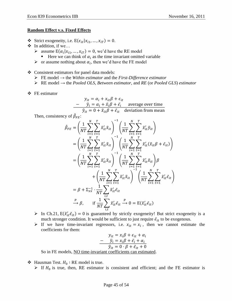
Random Effect v.s. Fixed Effects

Strict exogeneity, i.e. .

In addition, if we…

assume , we’d have the RE model

Here we can think of as the time invariant omitted variable

or assume nothing about , then we’d have the FE model

Consistent estimators for panel data models:

FE model → the Within estimator and the First-Difference estimator

RE model → the Pooled OLS, Between estimator, and RE (or Pooled GLS) estimator

FE estimator

Then, consistency of :

In Ch.21, is guaranteed by strictly exogeneity! But strict exogeneity is a

much stronger condition. It would be sufficient to just require to be exogenous.

If we have time-invariant regressors, i.e. , then we cannot estimate the

coefficients for them:

So in FE models, NO time-invariant coefficients can estimated.

Hausman Test. RE model is true.

If is true, then, RE estimator is consistent and efficient; and the FE estimator is


of 54

consistent (but not efficient).

Suppose is not true. Then, RE estimator is inconsistent; but FE estimator is consistent.

If is large, this is evidence against .

Let and be the time-variant estimates, where denotes variant regressors

So the test is

Homework:

Show that

Show that


of 54

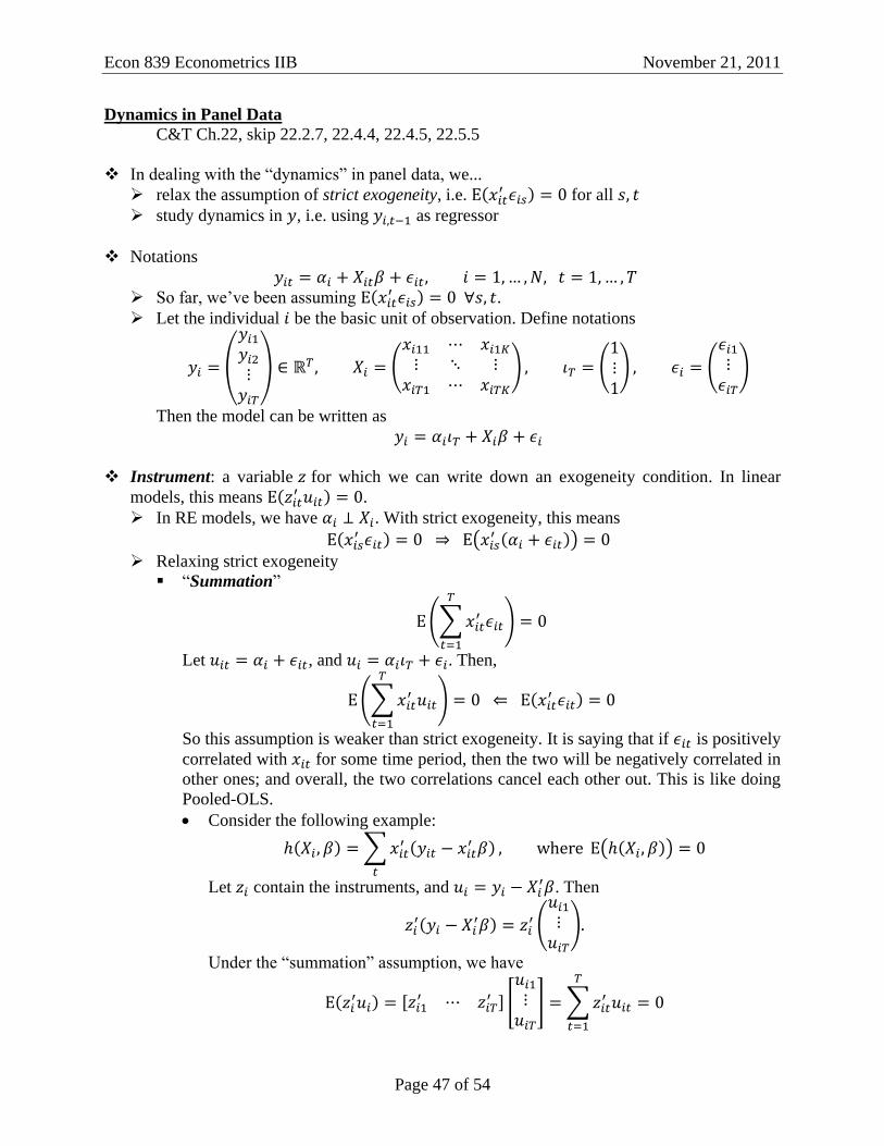
Dynamics in Panel Data

C&T Ch.22, skip 22.2.7, 22.4.4, 22.4.5, 22.5.5

In dealing with the “dynamics” in panel data, we...

relax the assumption of strict exogeneity, i.e. for all

study dynamics in , i.e. using as regressor

Notations

So far, we’ve been assuming .

Let the individual be the basic unit of observation. Define notations

Then the model can be written as

Instrument: a variable for which we can write down an exogeneity condition. In linear

models, this means .

In RE models, we have . With strict exogeneity, this means

Relaxing strict exogeneity

“Summation”

Let , and . Then,

So this assumption is weaker than strict exogeneity. It is saying that if is positively

correlated with for some time period, then the two will be negatively correlated in

other ones; and overall, the two correlations cancel each other out. This is like doing

Pooled-OLS.

Consider the following example:

Let contain the instruments, and . Then

Under the “summation” assumption, we have


of 54

Contemporaneous exogeneity

This implies “summation” (i.e. stronger than the “summation” assumption)

Over-identification: there are moment conditions but only parameters

Have to use GMM.

consider the example

Here is a matrix: since is so that

has to have columns

for the multiplication to be conformable; since there are moment conditions,

there has to be rows in . So that

where each is a vector.

The sample analog of the moment conditions

where

In GMM, the criterion function is

The FOC is

Weak exogeneity

This implies contemporaneous exogeneity, and hence also “summation”

This assumption is saying that current regressors are uncorrelated with future

error terms.


of 54

Construct matrix for moment conditions

where

Dynamic panels

, iid observations and fixed

if , i.e. no error terms are correlated across periods

, stationarity of

Weak exogeneity

Pooled-OLS

For the estimate to be consistent, we need . But clearly,

.Thus OLS estimate is inconsistent.

FE model

But notice that

and hence . Thus, the estimate is not consistent either.

First difference.

But this is still inconsistent, because contains which is correlated with , a

component of .

Homework: how do we solve this inconsistency problem in dynamic panel data models?


of 54

Dynamic Panel Data (cont’d)

Wrapping up dynamic panel data:

Note that and are strongly correlated.

Assume there’s no serial correlation. Then is a good instrument, and so are ,

, etc.

The moment condition is , where

Binary choice with panel data

In panel data,

Problem with :

Neglects unobserved heterogeneity

Problem with :

It is possible that Not consistent with economic theory:

Then the condition mean is

in which case we cannot isolate in the estimation.

Incidental parameter problem.

The likelihood function

and the log-likelihood

Take derivative w.r.t. and , and set them equal zero we get


of 54

This means when , will be 50% away from the true value, even if we allow

!!!

A possible solution for the case of logit. . The likelihood contribution is

Assume mutually independent . .

Condition on


of 54

Program Evaluation

Drop 25.4.5

Read 3.3, 3.4

There is a program (i.e. a treatment), and we’re trying to evaluate what kind of effect this treatment has.

Main problem with program evaluation: self-selection issue

In economics, it’s hard to conduct a “perfect experiment” with random assignment into treatment and control groups

Main application: labor and development

In the labor market programs, the self-selection issue is who chooses to enrol in these

programs: maybe those who expect to find a job after these programs would actually

enrol. On the other hand, it could also be that the program does have an effect on

improving the chance of the enrolled finding a job later; this is the treatment effect.

Essentially, program evaluation wants to disentangle these two effects.

The model

Fundamental problem of causal inference: we can see either or , i.e.

is the number of individuals. Among them have , i.e. the size of treatment group;

and is the size of control group. Data is .

What we are interested in

Average treatment effect.

This is the average treatment effect for the treated (or ATT or ATET)

Randomized Control Trial: , so that outcomes are independent of treatment.

Since , we infer that

By the LLN, is a consistent estimate of .

Two alternative assumptions

Unconfoundedness (or conditional independence): . This means that,

conditional on , outcomes are independent of treatment. But there is no test of


of 54

whether there is enough controls in the . This implies .

Overlap (or matching assumption): where for

all . This is saying that we are not sure whether or not somebody is in the treatment

group for a given value of . In other words, there are both treated and untreated

individuals for each . This way, we can compare treated and untreated individuals

for any given

To estimate the ,

Suppose , and for , let be the number of observations with

, and the number of observations with and .

Thus, consistently estimates .

This motivates

But this approach is hard to implement in practice because for each we need to have a

large number of observations (to have the convergence in probability). This means that

our dataset needs to be extremely large.

Propensity Score Matching (with unconfoundedness and overlap assumptions)

Propensity score: , where is estimable (e.g. from probit

or logit of on )

Instead of , look at

Note that

Suppose we have [we know that (

)], but after logit/probit,


of 54

Program Evaluation (cont’d)

C&T 25.6

Regression Discontinuity (RD)

Sample slightly to the left of the threshold is assumed to be almost identical to the sample

slightly to the right of the threshold. So by comparing the two samples, we get the effect

of the program.

Mathematically,

is a continuous variable with observation

is the threshold

Construct

Let the model be

where determines , and may be correlated with (thus so may ).

Since fully determines ,

Then the model can be rewritten as

Now . We can use

to approximate . So we can do OLS on this new equation. This is called the

control function approach.

Cohort size

Test scores

Effect of

program

econ 839 econometrics iib sept 12, 2011 - sfu.cahaiyunc/notes/econ 839 notes.pdf · econ 839...

Documents