Eco 610 Mathematical Economics I Notes M. Jerison 8/24/14

1. Introduction

Economists analyze qualitative relations (e.g., who is whose boss, or which ownershippattern is more efficient) and quantitative relations (e.g., prices, which are ratios of amountsof goods exchanged). Mathematics is a language for describing qualitative and quantitativerelations, so it is a natural language for economic analysis. Economists study effects ofpolicies and events using mathematical models to formulate counterfactual questions suchas “What would the euro/dollar exchange rate be now if the U.S. had defaulted on partof its debt in August 2011?” or, more generally, “What would have happened if a differentpolicy had been adopted or a different event had occurred?” The models are collectionsof sets along with relations among the elements of the sets. Counterfactuals have theform of logical implications: “If A, then B” (e.g., “If consumers had more income, thentheir total saving would be higher.”). An important part of economic analysis consists indiscovering which sets of hypotheses imply which interesting conclusions. This involvesfinding and proving theorems. That is why this course emphasizes proofs along with othermathematical tools. The main tools we work with are constrained optimization and systemsof equations. The main theorems in these subject areas are proved using methods of realanalysis, which will also be a topic of the course.

We begin with some concepts and notation in logic and set theory that are prerequisitesfor the course. The symbol � will be used to mean “is defined to be.” The name of anobject being defined will be written in boldface.

Logic

Items in a mathematical model are often labeled by letters. The letters in economic modelsusually represent variables that take numerical values, but they can represent other things.For example, a statement such as “Every student in Eco 610 last year got the grade A”might be labeled A. Statements can be combined to form other statements: “A or B,”or “A and B.” We are mainly concerned with whether statements are true or not. Thestatement “not A,” also written A, is an abbreviation for the statement “statement A isfalse”, which means “statement A is not true.” The statement “A and B” is true if andonly if A is true and B is true. The mathematical term “or” is inclusive. The statement“A or B” is true if and only if any one of the following holds:A is true and B is false; A is false and B is true; A is true and B is true.

If we want to exclude the last possibility, we must say “either A or B, not both.”

Implication: A ñ B means “[A is true and B is true] or [A is false]” and can be writtenB ð A. Other ways of saying the same thing: If A then B; B if A; A only if B; B isnecessary for A; A is sufficient for B; [(not Bq ñ (not A)]. This last implication is calledthe contrapositive of rAñ Bs. It is sometimes easier to prove an implication by provingits contrapositive. (Keep this in mind when you try to solve the exercises in these notes.)

The converse of Añ B is the statement B ñ A. Note that Añ B may be true and itsconverse false, or Añ B may be false and its converse true. (Prove these claims.)

If A ñ B and its converse, B ñ A, are both true, we say that A is equivalent to B orthat A and B are equivalent. Then we write A ô B, which means “[A is true and B istrue] or [A is false and B is false].” There are many other ways to say or write the samething: A if and only if B; A iff B; A is necessary and sufficient for B.

1

2

If the statement A ñ B is true, it is called a theorem. One of the main problems ofeconomic analysis is to determine which implications are theorems when A and B containinteresting statements about economic relations. The main way of convincing people that atheorem is a theorem is to break it into a sequence of statements Ai ñ Ai�1, i � 1, 2, . . . , nthat are each accepted as true, with A � A1 and B � An�1. The intermediate statementsAi may be theorems and axioms from mathematics or from an economic model. Thesequence is called a proof. Examples are given in these notes, in SB pp. 851–858, and inthe books by Solow and Velleman in the syllabus.

In ordinary English there are statements that are neither true nor false, e.g., “This state-ment is false.” Standard logical systems in mathematics avoid this by allowing statementsto refer only to a fixed “universal” set of objects and to sets constructed from subsets ofthat set through mathematical grammar. In that case, the sentence in quotes, above, isnot a statement. On the other hand, in mathematical logic systems that include basicarithmetic, some statements are undecidable, i.e., impossible to prove or disprove (Godel(1931)). The most important examples of these statements deal with infinite sets. So farin economics, this issue has only come up in a narrow part of game theory.

Some Sets and Notation

A collection of objects is called a set. The objects are called elements or members ofthe set. If x is an element or member of a set S, we write x P S and say that x is in S.

A set can be defined by enumeration (listing of its elements): tAlbany, Schenectady, Troyu,or by partial enumeration, when the pattern is clear:N � t1, 2, 3, . . . u, the set of natural numbers,P � t2, 3, 5, 7, 11, 13, 17, . . . u, the set of prime numbers,Z � t0, 1,�1, 2,�2, 3,�3, . . . u, the set of integers.Q � the set of rational numbers or rationals,R � the set of real numbers or reals.H � the empty set (with no elements).

Alternatively, sets can be defined by properties that their elements satisfy, e.g.,the set of even integers � tn P Z : n � 2k for some k P Zu � t2k : k P Zu,where : means “such that”.

Sets can be defined from operations involving other sets: X � S Y T � union of Sand T ; Y � S X T � intersection of S and T ; SzT � tx : x is in S and not in T u �complement of T in S. It is denoted zT or T c if the set S is understood.

S � T means that every element of the set S is also an element of T . If it is true, we saythat S is a subset of T or is contained in T , and we also write T � S. Two sets S andT are equal (and we write S � T ) if they have exactly the same elements, in other words,if every element of S is also an element of T and vice versa (so S � T and T � S). S is aproper subset of T if S � T , but S � T .

The set of subsets of a set S is called the power set of S. The set C � tcu with the singleelement c has two different subsets. (What are they? What is the power set of C?)The power set of a set S is denoted 2S. (Why?)

X �Y is the set of ordered pairs px, yq with x P X and y P Y . We use the term “orderedpair” to refer to the fact that px, yq is treated as different from py, xq if x � y.

3

Let Sα be a set for each α in a set A. The set A is called an index set and an element ofA is an index. The set of sets Sα is called a collection of sets.YαPASα � tx : x P Sα for some α P Au is the union of the sets Sα. We write Ynα�1Sα IfA � t1, 2, . . . , nu.XαPASα � tx : x P Sα for every α P Au is the intersection of the sets Sα.The symbol α used for an index can be replaced by any other symbol: YαPASα � YβPASβ.

A collection of sets is disjoint if every pair of sets in the collection has empty intersection.A partition of a set S is a disjoint collection of nonempty subsets of S with union S.

Important sets:ra, bs � R, the closed interval tx P R : a ¤ x ¤ bu, a ¤ b.pa, bq � R, the open interval tx P R : a   x   bu. Note: a could be �8; b could be 8.ra, bq � tx P R : a ¤ x   bu, pa, bs � tx P R : a   x ¤ bu are half open intervals, neitheropen nor closed. An interval that is not open need not be closed. An interval that is notclosed need not be open.R� � tx P R : x ¥ 0u � r0,8q, the nonnegative real numbersR� � tx P R : x ¤ 0u � p�8, 0s, the nonpositive real numbersR�� � tx P R : x ¡ 0u, the positive real numbersR�� � tx P R : x   0u, the negative real numbers

Identities: AX pB Y Cq � pAXBq Y pAX Cq; AY pB X Cq � pAYBq X pAY Cq;DeMorgan’s Laws: zpAY Cq � pzAq X pzCq; zpAX Cq � pzAq Y pzCq.@ means “for each” or “for all.”

D means “there exists.” Example: @a P R, Dx P R : x ¡ a.

D1 means “there exists exactly one.” Example: @n P N, D1m P N : m � n� 1.

A slash through a symbol means “not,” as in �, R, �, E.Example: @n P N, Em P N : n   m   n� 1.°

, addition symbol:°3i�1 ai � a1 � a2 � a3;

°ni�2 ai � a2 � a3 � a4 � � � � � an.

Π, product symbol: Πni�1ai � a1 � a2 � a3 � � � � an, where each ai P R.

an � a � a � � � � � a � “a to the power n” (a multiplied by itself n times, where a P R, n P N).

n! � n � pn� 1q � � � 2 � 1 � n factorial for n P N. Also 0! � 1.

Πni�1Si � S1 � S2 � S3 � � � � Sn � tpx1, x2, . . . , xnq : xi P Si, i � 1, . . . , nu is the product of

the sets Si, with n P Z or n � 8. An element of Πni�1Si is a list or an n-tuple.

Sn � Πni�1Si, where Si � S, i � 1, . . . , n

p P N is prime if p ¡ 1 and p is divisible only by p and 1 in N (p � mn for m,n P Nimplies m � 1 or n � 1.) Important property of the natural numbers: Every m P N(m ¡ 1) has a unique prime factorization: There is a unique list of prime numbers pi andnatural numbers ni, i � 1, . . . , I, such that pi   pi�1 for i � 1, . . . , I � 1, and m � ΠI

i�1pnii .

sign a � 1 if a ¡ 0. sign a � 0 if a � 0. sign a � �1 if a   0.

|a| � psign aqa � absolute value of (magnitude of) a P R; |S| � # elements in set S.

The statement°ni�1 i � npn� 1q{2 depends on the index n P N. We can label it Spnq.

4

Mathematical Induction: Every statement P pnq for n P N, n ¥ m, is true if the followingconditions are satisfied: (a) P pmq is true; (b) for every k P N with k ¥ m, P pk�1q is true ifP pkq is true. The assumption that P pkq is true in (b) is called the induction hypothesis.The statement Spnq above is proved by induction for all n P N in SB pp. 856–857.

ExercisesX1. Prove that if m balls are put in n boxes (n   m), then at least one box contains morethan one ball.X2. Prove that Πn

i�1p1� aiq ¥ 1�°ni�1 ai if ai P R�, @i.

X3. The following argument claims to prove that all people are of the same sex. Findthe first sentence that contains an incorrect step in the argument and explain clearly themistake(s) in it.“Proof”: Call a set of people uniform if all the people are of the same sex. We want to provethat every set of k people is uniform for each k P N. The conclusion is correct for k � 1.Next, suppose that every set of k people is uniform. (This is the induction hypothesis.)We must prove that every set of k � 1 people is uniform. Start with k � 1 people andremove one person. The remaining set of people is uniform by the induction hypothesis.Now bring the removed person back and remove someone else. Again, the set of remainingpeople is uniform. So the set of k � 1 people is uniform and the claim is proved.X4. Consider a set of n people and assume that no person is her or his own friend andthat whenever person A is a friend of person B, B is a friend of A. Is it possible that notwo people in the set have the same number of friends in the set? Hint: Try to answer thiswithout using induction. Consider the number of friends different people in the set musthave if they all have different numbers of friends.

Relations, Functions and Correspondences

This section develops terminology and notation for studying economic relations. We mightwant to ask, for example, which people are members of the boards of directors of whichfirms, or ask if one nation is wealthier than another, or if a consumer prefers one bundle ofgoods to another. These are all examples of relations. To specify a relation formally, weneed to specify which elements x of some set X are related to which elements y of a setY . The pairs px, yq that are related in this way are identified as being elements of some setR � X � Y . The relation is identified with the set R. When px, yq P R, we say that x isrelated to y under R and write xRy.

Example 1. A relation between board members and firms can be specified by listing po-tential members, labeled A, B, C and D, and firms, labeled 1, 2 and 3. The relationtpA, 1q, pA, 2q, pB, 2q, pC, 1q, pC, 3q, pD, 1q, pD, 3qu is interpreted as specifying that firm 1has A, C and D on its board, firm 2 has A and B, and firm 3 has C and D.

Example 2. A (weak) preference relation on a set X is a subset © of X � X that isreflexive px © x, @x P Xq and transitive px © y and y © z ñ x © z, @x, y, z P Xq.Example 3. An equivalence relation E on a set X is relation that is reflexive, transitive,and symmetric pxEy ñ yEx,@x, y P Xq. In the theory of the consumer, indifference(between bundles of goods) is an equivalence relation. Every partition tSiuiPI of a set Xdetermines an equivalence relation E in which xEy iff x and y are in the same Si � X.(Prove this last claim.) An equivalence class of an equivalence relation E on X is aset S � X such that xEy,@x, y P S.

5

Example 4. A rational number is a ratio of integers m and n. But what is a ratio? We candefine the rationals formally by associating m{n with the integer pair pm,nq where n � 0.But then the same rational number is also associated with pkm, knq for any integer k � 0(since km{pknq � m{n. Thus, formally, each rational number m{n must be defined as anequivalence class of pairs of integers for an equivalence relation � such that pm,nq � pp, qqwhenever mq � np for integers n � 0, q � 0, m, and p.

One of the most important relations is the functional relation. Many textbooks call afunction f a “rule” that assigns to each element of a set X a unique element of a set Y .This is expressed by writing f : X Ñ Y or x P X ÞÑ fpxq P Y . The set X is called the“domain” or “source.” The set Y is called the “range” or “target” of the function. Butwhat is a rule? Can we define what it means for something to be a function, using onlyterms that have a clear meaning? The answer is yes. The rule is specified by the graph ofthe function, the set of pairs px, yq P X � Y that the function associates with each other.But the function itself is more than its graph.

Example: Each hand in the classroom belongs to a unique person. This defines a functionwith domain the set of hands in the room and range the set of people in the room. Thesame relation can be represented by other functions simply by making the range a largerset. For example, the domain could be the set of hands in the room and the range couldbe the set of people in the world. It is important to distinguish between these functions.The function associates hands in the room to people in the room is “onto” (every person inthe range of the function has a hand in the domain), whereas the function that associateshands in the room to people in the world is not onto.

X5. Give a formal definition of the term function. Define a function to be a list of setssatisfying some restriction(s). Your definition must include everything that determines afunction and nothing extra. That way, two lists of sets satisfying your restrictions representthe same function if and only if they are the same list. Your definition should not includeany undefined terms except for the names of the sets in the list.

An element gpxq of Y , the unique element of Y assigned by the function g : X Ñ Y tosome x in X is called a value of g. The function is called real-valued if Y � R. Anelement of the domain is called an argument of the function. The set of values assignedto arguments in S � X is gpSq � ty P Y : px, yq P G for some x P Su, called the image ofg on S. It is simply called the image of g if S � X, and is denoted Imageg or Img. Thepreimage or inverse image of V � Y under g is g�1pV q � tx P X : gpxq P V u, the setof arguments assigned values in V . The letters used to label the domain, range and graphof a function do not matter. What matters are the sets themselves.

The restriction of f : X Ñ Y to S � X (also called f on S) is the function f |S from Sto Y , defined by f |Spxq � fpxq, @x P S.

A function f : X Ñ Y is injective (or one-to-one) if fpxq � fpyq implies x � y; differentarguments are assigned different values by the function.A function f : X Ñ Y is surjective or onto if Imagef � Y , i.e., if every y P Y equals fpxqfor some x P X.A function that is injective and surjective is bijective (a one-to-one correspondence). Abijective f : X Ñ Y has a unique inverse f�1 : Y Ñ X with f�1pfpxqq � x, @x P X.

A set X is finite if there is a bijective f : X Ñ t1, 2, . . . , nu for some n P N. Then this nis the number of elements in X and is called the cardinality of X and is denoted |X| or

6

#X. A set that is not finite is infinite. Sets X and Y (finite or infinite) have the samecardinality if there is a bijection between them. Y has higher cardinality than X ifthere is an injection from X to Y but not from Y to X. A set is countable if there isa bijection between it and N. The set Q of rationals is countable. The set R of reals isnot; it has higher cardinality than N and Q. This follows from two facts: (1) R has thecardinality of 2N; (2) every set has lower cardinality than its power set.

X6. Prove that cardinality of a finite set is well-defined (defined without ambiguity) byproving that there cannot be two one-to-one correspondences f : X Ñ t1, 2, . . . , nu andg : X Ñ t1, 2, . . . ,mu with m � n.X7. Prove that a set is infinite iff it has the same cardinality as one of its proper subsets.

A permutation of a finite set can be thought of as a listing of the elements of the set in aparticular order. For example, one permutation of the set t1, 2, 3u is p1, 2, 3q and anotheris p3, 2, 1q. (Are there others? If so, what are they?) Formally, a permutation of theset S with #S � n is a bijection π : t1, 2, . . . , nu Ñ S. The function π determines the list,with πp1q P S coming first, followed by πp2q, etc.

X8. Prove that every set of n P N elements has n! different permutations.

A k-combination from a set S is a set of k distinct elements of S. For 1   k   n,there are

�nk

� � n!{rk!pn � kq!s different k-combinations from a set of n elements. The

definition 0! � 1 makes the same formula hold when k � n and k � 0. The number�nk

�is

referred to as “n choose k” or “n take k”. To see why the formula for it is correct, notethat every permutation of a set S of n elements is a listing of k distinct elements of Sfollowed by a listing of the n� k remaining elements. For each k-combination from S andeach permutation of these k elements, followed by any permutation of the n� k remainingelements, we get a distinct permutation of S. Therefore the number of permutations of Sis�nk

�k!pn� kq! � n!, which yields the formula above.

Binomial Theorem. px� hqn � °nk�0

�nk

�xkhn�k for x, h P R, n P N.

X9. (a) Prove that�nk

�� � nk�1

� � �n�1k

�for n P N and k � 1, . . . , n.

(b) Use induction to prove the binomial theorem.

A sequence in a set S is a function f : M Ñ S, where M is an infinite subset of N.Alternative notation for such a sequence: txiuiPM or txiu8i�1 if M � N, or txiui, wherexi � fpiq P S for i PM .

The composition or composite of f : X Ñ Y and g : W Ñ X 1 with Im g � X is thefunction f � g with domain W and range Y , defined by f � gpxq � fpgpxqq, @x P W .

Example: g : RÑ R, gpxq � 3x� 1. Note that this function could have been defined justas well by g : R Ñ R, gp�q � 3� � 1, or by gp3x � 1q � 3p3x � 1q � 1 � 9x � 2. It is the“rule” (determined by the graph of g) that matters, not the symbol used for the argument.The formula gpxq � 3x � 1 alone is not quite a complete definition of a function since itdoes not specify the domain (the set of x’s) or the range (set of y’s). By convention, we willassume that the domain is the largest set for which the formula is defined (unless specifiedotherwise). The function g in this example is affine, i.e., of the form:Gpxq � ax� b for x P R. The graph of an affine function on R is a straight line.

x P R ÞÑ fpxq � sinx does not completely specify a function since the range is notdetermined. The function is onto only if the range is r�1, 1s.

7

YaPASa � tx : x P Sa for some a P Au. XaPASa � tx : x P Sa, @a P Au.ΠaPASa � tpxaqaPA : xa P Sa, @a P Au.

The Real Numbers

To obtain conditions under which solutions to optimization problems exist, we need todescribe formally the properties of the set of reals R. We can define R as a set satisfyingthe following five axioms.

a1. R contains the set of rational numbers Q.

a2. The properties of addition, multiplication and order for Q also apply to R. For allx, y, z P R, addition and multiplication areassociative: px� yq � z � x� py � zq and pxyqz � xpyzq;commutative: x� y � y � x and xy � yx;distributive: xpy � zq � xy � xz; withx� 0 � x, x � 0 � 0, x� p�xq � 0, and for x � 0, x � p1{xq � 1.

a3. If x   y then x� z   y � z. If, in addition, z ¡ 0 then xz   yz.

a4. If x   y then there is a rational number q with x   q   y.

An upper bound [respectively, lower bound] for a set S � R is a number b P R suchthat b ¥ x [resp. b ¤ xs for every x P S. A least upper bound for S is an upperbound b for S such that no upper bound for S is less than b. A least upper bound for S iscalled the supremum of S and denoted supS. A greatest lower bound for S is a lowerbound b for S such that no lower bound for S is greater than b. A greatest lower boundfor S is called the infimum of S and denoted inf S. Example: For a, b P R with a   b,supra, bq � b. So supS is not necessarily an element of S. If S has no upper bound, thensupS � 8. If S � H then supS � �8.

a5. Every nonempty set of reals with an upper bound has a real least upper bound.

Axiom a5 ensures that the set of real numbers has no holes. This distinguishes the realsfrom the rationals. There are numbers such as

?2 that can be approximated arbitrarily

closely by rationals yet are not rational. Axiom a5 does not hold if the set of reals isreplaced by the set of rationals. The set of rationals less than

?2 has an upper bound, but

no least upper bound that is rational.

Exercises:

X10. Prove that for each p P P,?p is not rational (i.e., it is not the ratio of two integers).

X11. Use the axioms above to prove that x ¡ y implies �x   �y for x, y P R.X12. Use the axioms above to prove that every nonempty set of reals with a lower boundhas a unique infimum.

2. Basic Calculus

Topics: Limits, derivatives, monotone functions, monotonicity gap, exponents, logs, elas-ticity, chain rule, critical points, maximizers, minimizers, inflection points, first and secondorder conditions, convex sets, concave and convex functions, antiderivatives, integrals.SB chs. 2–5, 21 pp. 505–511, Appendix A4.

8

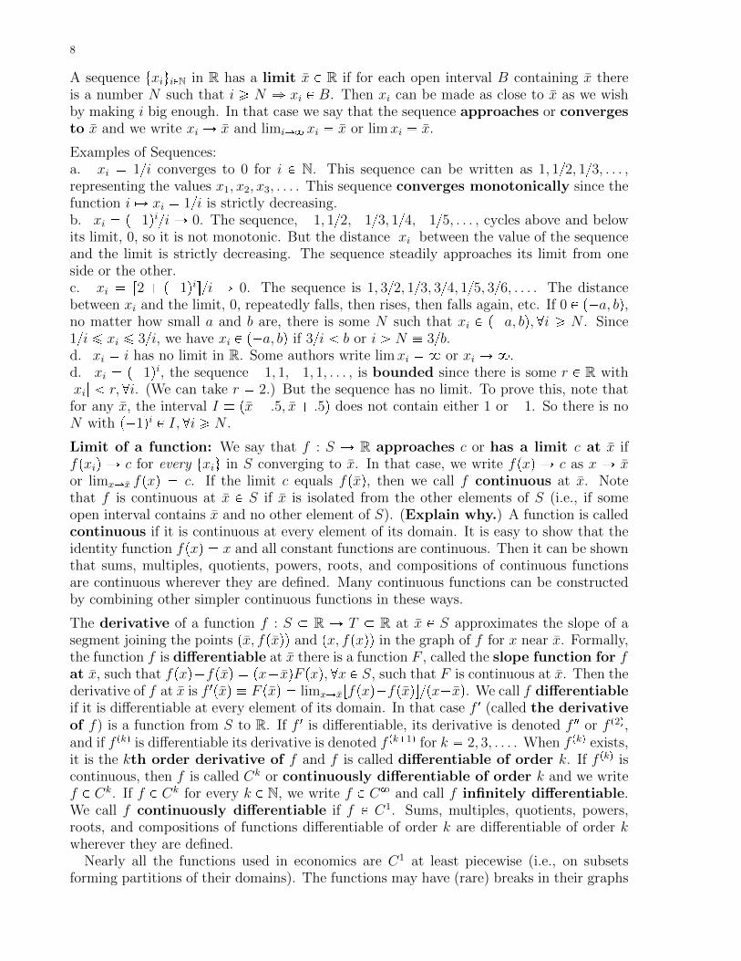
A sequence txiuiPN in R has a limit x P R if for each open interval B containing x thereis a number N such that i ¥ N ñ xi P B. Then xi can be made as close to x as we wishby making i big enough. In that case we say that the sequence approaches or convergesto x and we write xi Ñ x and limiÑ8 xi � x or lim xi � x.

Examples of Sequences:a. xi � 1{i converges to 0 for i P N. This sequence can be written as 1, 1{2, 1{3, . . . ,representing the values x1, x2, x3, . . . . This sequence converges monotonically since thefunction i ÞÑ xi � 1{i is strictly decreasing.b. xi � p�1qi{i Ñ 0. The sequence, �1, 1{2,�1{3, 1{4,�1{5, . . . , cycles above and belowits limit, 0, so it is not monotonic. But the distance |xi| between the value of the sequenceand the limit is strictly decreasing. The sequence steadily approaches its limit from oneside or the other.c. xi � r2 � p�1qis{i Ñ 0. The sequence is 1, 3{2, 1{3, 3{4, 1{5, 3{6, . . . . The distancebetween xi and the limit, 0, repeatedly falls, then rises, then falls again, etc. If 0 P p�a, bq,no matter how small a and b are, there is some N such that xi P p�a, bq, @i ¥ N . Since1{i ¤ xi ¤ 3{i, we have xi P p�a, bq if 3{i   b or i ¡ N � 3{b.d. xi � i has no limit in R. Some authors write limxi � 8 or xi Ñ 8.d. xi � p�1qi, the sequence �1, 1,�1, 1, . . . , is bounded since there is some r P R with|xi|   r,@i. (We can take r � 2.) But the sequence has no limit. To prove this, note thatfor any x, the interval I � px � .5, x � .5q does not contain either 1 or �1. So there is noN with p�1qi P I,@i ¥ N .

Limit of a function: We say that f : S Ñ R approaches c or has a limit c at x iffpxiq Ñ c for every txiu in S converging to x. In that case, we write fpxq Ñ c as x Ñ xor limxÑx fpxq � c. If the limit c equals fpxq, then we call f continuous at x. Notethat f is continuous at x P S if x is isolated from the other elements of S (i.e., if someopen interval contains x and no other element of S). (Explain why.) A function is calledcontinuous if it is continuous at every element of its domain. It is easy to show that theidentity function fpxq � x and all constant functions are continuous. Then it can be shownthat sums, multiples, quotients, powers, roots, and compositions of continuous functionsare continuous wherever they are defined. Many continuous functions can be constructedby combining other simpler continuous functions in these ways.

The derivative of a function f : S � R Ñ T � R at x P S approximates the slope of asegment joining the points px, fpxqq and px, fpxqq in the graph of f for x near x. Formally,the function f is differentiable at x there is a function F , called the slope function for fat x, such that fpxq�fpxq � px� xqF pxq, @x P S, such that F is continuous at x. Then thederivative of f at x is f 1pxq � F pxq � limxÑxrfpxq�fpxqs{px�xq. We call f differentiableif it is differentiable at every element of its domain. In that case f 1 (called the derivativeof f) is a function from S to R. If f 1 is differentiable, its derivative is denoted f2 or f p2q,and if f pkq is differentiable its derivative is denoted f pk�1q for k � 2, 3, . . . . When f pkq exists,it is the kth order derivative of f and f is called differentiable of order k. If f pkq iscontinuous, then f is called Ck or continuously differentiable of order k and we writef P Ck. If f P Ck for every k P N, we write f P C8 and call f infinitely differentiable.We call f continuously differentiable if f P C1. Sums, multiples, quotients, powers,roots, and compositions of functions differentiable of order k are differentiable of order kwherever they are defined.

Nearly all the functions used in economics are C1 at least piecewise (i.e., on subsetsforming partitions of their domains). The functions may have (rare) breaks in their graphs

9

or may have kinks. A kink is a point in the graph where the function is continuous, butnot differentiable. For the most commonly used functions in economics, derivatives can bedefined without using limits. Let such a function f be differentiable at x. For h near 0,there is a continuous function g satisfying hgpx, hq � fpx�hq�fpxq. Then f 1pxq � gpx, 0q.For example, let fpxq � x2. Then fpx� hq � fpxq � px� hq2 � x2 � 2xh� h2 � hgpx, hq,where gpx, hq � 2x� h. So f 1pxq � gpx, 0q � 2x.

A real-valued function f is nondecreasing on a set S � R if for x, y P S, x ¡ y impliesfpxq ¥ fpyq. The function is nonincreasing on S if for x, y P S, x ¡ y implies fpxq ¤ fpyq.The function is strictly increasing, [respectively, strictly decreasing] on S if for x, y P S,x ¡ y implies fpxq ¡ fpyq [resp., fpxq   fpyq]. We omit reference to S (and say that f isnondecreasing, strictly increasing, etc.) if S is the entire domain of f . A function is calledweakly monotone if it is nondecreasing or nonincreasing. It is called monotone if it isstrictly increasing or strictly decreasing. Some authors use the term monotone to meanstrictly increasing alone.

A differentiable function f : S Ñ R with S � R is nondecreasing [respectively, nonincreas-ing] if and only if f 1 ¥ 0 [f 1 ¤ 0]. (Note that f 1 ¥ 0 means that f 1pxq ¥ 0 for every xin the domain of f .) Thus the sign of the derivative can tell us if the function is weaklymonotone. If f 1 ¡ 0 then f is strictly increasing. If f 1   0 then f is strictly decreasing.However the converses of these two statements are false. In particular, f 1 ¡ 0 might not betrue when f is strictly increasing. (Prove this.) I call this fact the monotonicity gapreferring to the gap between the condition of having a positive derivative and the weakercondition of being strictly increasing. If f is nondecreasing, then it is differentiable exceptat “rare” points (to be defined below). If f is strictly increasing, f 1pxq may be 0, but onlyat rare x. (Certainly not on any open interval, because then f is constant on that interval.)

Convexity plays an central role in economic theory as a way of representing “decreasingreturns” from changes in production or consumption. A set in Rn is convex if it containsevery segment that has endpoints in the set. A function f : X � Rn Ñ R is convex ifthe set of points px, yq with y ¥ fpxq, i.e., the set of points lying on or above its graph isconvex. (Note that these are not quite complete definitions since we have not yet defineda segment.) The function f is concave if the set of points px, yq with y ¤ fpxq (the set ofpoints on or below the graph of f) is convex. Note that we do not speak of concave sets.These definitions are geometric. We will give algebraic versions of them and generalizethem to functions of several variables below.

1. A differentiable function f : R Ñ R is convex rrespectively, concaves if and only if f 1

is nondecreasing rrespectively nonincreasings. If f is twice differentiable, then it is convexrrespectively, concaves if and only if f2 ¥ 0 rf2 ¤ 0s.

These characterizations of convex and concave functions using derivatives apply onlyto functions of a single real variable. Versions for functions of several variables will bediscussed below. Note that convex and concave functions need not be differentiable. Theirgraphs can have kinks. But they are differentiable except at “rare” points. We will statethis more precisely later.

A function f : X � Rn Ñ R is strictly convex [respectively, strictly concave] if forevery segment with distinct endpoints in the graph of f , the other points of the segmentare above [respectively, below] the graph of f .

10

2. A differentiable function f : RÑ R is strictly convex rrespectively, strictly concaves if f 1

is increasing rrespectively decreasings. If f is twice differentiable, then it is strictly convexrrespectively, strictly concaves if f2 ¡ 0 rf2   0s.

The converses of these statements are false. For example, a twice differentiable, strictlyconcave function f : RÑ R might not satisfy f2   0. It is possible that f2pxq � 0 at somevalue(s) of x. (X Find an example of such a function.) But if f is twice differentiable andstrictly concave, we cannot have f2pxq � 0 for all x in an open interval.

In section 12 we define an exponential function fpxq � bx with base b ¡ 0, for x P R.We prove that it has the following important properties:E1. If x P N, then fpxq is b multiplied by itself x times.E2. f is positive and has a positive derivative of every order.E3. fpx� yq � fpxqfpyq.E4. fpxyq � bxy � pbxqy � pbyqx.The limit limnÑ8r1� p1{nqsn exists and equals

°8n�0p1{n!q, and is denoted e � 2.71828. If

fpxq � ex, then f 1 � f .

fpxq � bx has an inverse function, the logarithmic function logb x, with these properties:L1. logb fpxq � x and fplogb xq � x.L2. logb xy � logb x� logb y.L3. logb x

y � y logb x.The natural log function is ln x � logex.L4. If gpxq � logb x, then g1pxq � 1{px ln bq.These functions are important in economics because the growth rates of so many economicvariables do not change drastically over time. The growth rate of a differentiablefunction f at x is f 1pxq{fpxq. If f is the exponential function bx above, then its growthrate at x is f 1pxq{fpxq � ln b for all x. Exponential functions have constant growth rates.

X13. Use properties E1, E2, E3, E4, L1, L2, L3 to prove that fpxq � bx satisfies fp0q � 1,fp�yq � 1{fpyq and fpxq{fpyq � fpx� yq, and that logbpx{yq � logb x� logb y.

A differentiable function f : S Ñ R with S � R has elasticity xf 1pxq{fpxq at x wherefpxq � 0. The elasticity measures the response of the function to variations in its argument.It is especially useful for economic applications since it is unaffected by changes in the unitsin which the variables in the domain and range of the function are measured. To see whythis is true, first consider a change of units for elements of the range of the function. Thishas the effect of multiplying the value of the function by a constant, say k. The elasticityat x is then xkf 1pxq{rkfpxqs � xf 1pxq{fpxq. Suppose instead that the units in which theargument of the function change. Let the unit size be divided by k. Then x units become kxunits. The function with these new units is F , where F pkxq � fpxq. Since kF 1pkxq � f 1pxq,we see that xf 1pxq{fpxq � kxF 1pkxq{F pkxq. The elasticity of F at the correct argumentkx, which represents the same quantity in the new units as x in the old, is the same theelasticity of f at x.

The Darboux-Stieltjes Integral: This integral provides a general notation for expectedvalues of discrete or continuous random variables. Consider a nondecreasing function F :ra, bs Ñ R, where a   b P R and F paq   F pbq. Define F pt�q � suptF pxq : x   tu for t ¡ aand F pt�q � inftF pxq : x ¡ tu for t   b, and let F pa�q � F paq and F pb�q � F pbq. If F iscontinuous at t, then F pt�q � F ptq � F pt�q. Otherwise, F pt�q�F pt�q is called the jump ofF at t. Let f : ra, bs Ñ R be bounded. For S � ra, bs, define Mpf, Sq � suptfpxq : x P Su

11

and mpf, Sq � inftfpxq : x P Su. Call P � ptiqni�0, with a � t0   t1   � � �   tn�1   tn � b,a division of ra, bs. (It is sometimes called a partition, but it is not a set of subsets ofra, bs.) Define JF pf,Pq � °n

k�1 fptkq � rF pt�k q � F pt�k qs, and the

upper sum: Upf,Pq � JF pf,Pq �n

k�1

Mpf, rtk�1, tksq � rF pt�k q � F pt�k�1qs and

lower sum: Lpf,Pq � JF pf,Pq �n

k�1

mpf, rtk�1, tksq � rF pt�k q � F pt�k�1qs

of f for F on P . Define UF pfq � inftUpf,Pq : P a division of ra, bsu and LF pfq �suptLpf,Pq : P a division of ra, bsu. It can be shown that UF pfq ¥ LF pfq. If these terms

are equal, their value is called the F -integral of f and is denoted³bafdF or

³bafpxqdF pxq;

then the function f is called F -integrable on ra, bs. The subscript a and superscript b on³are called limits of integration and may be omitted when it does not cause confusion.

A function f is called piecewise continuous on a subset of R if it is continuous at all butfinitely many points of its domain.

Theorem 1. If a function is piecewise continuous or if it is bounded and either nonde-creasing or nonincreasing then it is F -integrable.

More general F -integrable functions can be constructed by piecing together functionsthat are nondecreasing or nonincreasing on adjacent intervals. Functions that are notF -integrable are unbounded or have too many discontinuities.

Theorem 2. Let f and g be F -integrable and G-integrable functions on ra, bs. For c P R,(a)

³pcf � gqdF � cp³ fdF q � ³ gdF ,(b) | ³ f dF | ¤ ³ |f |dF ,(c)

³fdpF �Gq � ³ f dF � ³ fdG,

(d) f ¤ g ñ ³f dF ¤ ³ g dF , and

(e) if g is continuous and F is C1, then³g dF � ³b

agpxqF 1pxqdx.

The next result generalizes integration by parts and the Fundamental Theorem of Calculus.

Theorem 3. Integration by Parts: Let F and G be nondecreasing on ra, bs, and define

F �ptq � rF pt�q � F pt�qs{2 and G�ptq � rGpt�q �Gpt�qs{2, @t P ra, bs.Then

³baF �dG� ³b

aG�dF � F pbqGpbq � F paqGpaq.

X14. Use theorems 2(e) and 3 to prove³baF 1pxqdx � F pbq � F paq for F P C1 with F 1 ¥ 0

on ra, bs.If³baf dF exists for every interval ra, bs � R and the limits limbÑ8

³b0f dF and limaÑ�8

³0af dF

both exist, then the improper integral³R f dF is defined to be the sum of those two limits.

Integrals on unions of disjoint intervals are defined as sums of the integrals on the intervals.If S � T , then an integral on T zS � tx P T : x R Su equals the integral on T minus theintegral on S. Applying these definitions we can define

³Sf dF for any set S constructed

by countable unions and finite intersections of intervals in R.Given g : R Ñ R and a real valued random variable X with distribution function F

(where F pxq is the probability that X takes a value no greater than x), the expected valueof gpXq is

³R g dF , denoted EgpXq. The expected value of gpXq conditional on X taking a

value in a set S is ErgpXq|X in Ss � p³Sg dF q{p³

SdF pxqq, also denoted ErgpXq|Ss.

12

3. Vectors, Functions of Several Variables and Their Derivatives

We want to study functions that depend on several variables, or more generally studymodels in which the values of some variables are determined by values of others. It isconvenient to treat each set of variables as a single object called a vector. A vector can bethought of as an abstract object, an element of a vector space, but we will start out withthe most important examples of vectors, elements of Euclidean space, Rn, represented aslists of n real numbers px1, x2, . . . , xnq (also written pxiqni�1 or pxiq). The list is called ann-vector and a number xi in the list is called a component or entry or element of thevector. We interpret each n-vector as a “displacement,” i.e., a direction and a length. Adisplacement can be represented geometrically as an arrow with a base point and a “tip.”Arrows with the same direction and length but different base points represent the samevector.

Example A. We may treat the quantities of goods bought by a group of consumers asdepending on the consumers’ incomes and the prices of all the goods. The lists of quantitiesof goods, of prices and of consumer incomes are all vectors.

Vectors can be added can be added to each other and can be multiplied by scalars (realnumbers). The sum of the vectors x � px1, x2, . . . , xnq and y � py1, y2, . . . , ynq is x � y �px1 � y1, x2 � y2, . . . , xn � ynq. Multiplying t P R by y yields ty � pty1, ty2, . . . , tynq. Thereis a unique vector 0 such that 0�x � x for every vector x, and for each vector y, there is aunique vector �y such that �y�y � 0. Vector addition is commutative px�y � y�xq andassociative px � yq � w � x � py � wq. Scalar multiplication satisfies the distributive law,tpx�yq � tx�ty, and is associative, tpuyq � ptuqy, for t, u P R. Be sure you understand thegeometric interpretation for these operations. (See SB ch. 10.) For example, the negativeof a vector has the same length and points in the opposite direction.

Two vectors are called collinear if one is a scalar multiple of the other. Draw pictures ofexamples of collinear vectors and convince yourself that they point in the same or oppositedirection (from 0). If two vectors x and y are not collinear, then they determine a plane(the plane determined by the three points x, y and 0). Each point in this plane can bewritten as αx � βy, for some α and β in R. Such a vector is called a linear combinationof x and y. More generally, a linear combination of a set of K vectors tvkuKk�1 is a

vector°Kk�1 αkvk, where each αk is real. The set of linear combinations of the vectors vk is

called their span and denoted span tvku.The dot product (or inner or scalar product) of the vectors x � px1, x2, . . . , xnq andv � pv1, v2, . . . , vnq in Rn is x � v � °n

i�1 xivi, also written xv. The length or Euclideannorm of x is }x} � ?x � x. The set Rn with this norm is called n-dimensional Euclideanspace. (Other norms can be defined and used for various purposes, e.g., the sup norm,}x}8 � maxt|x1|, |x2|, . . . , |xn|u. The term “space” refers to a set with additional structure,in this case, sums, products and norms.) The dot product and norm satisfy the followingidentities for all vectors x, v and w in Rn and scalars t, τ P R:x � v � v � x, ptxq � v � x � ptvq � tpx � vq, x � pv � wq � px � wq � px � wq,}x} ¥ 0, r}x} � 0 ñ x � 0s, }tx} � |t|}x} and }x� v} ¤ }x} � }v}, the triangle inequality.

A function f : Rn Ñ Rm is called linear if fpx � yq � fpxq � fpyq and fptxq � tfpxq forall x, y P Rn and t P R. A linear function f : Rn Ñ R can be written as fpxq � a � x forsome vector a. This class of functions generalizes the class of functions from R to R thathave straight line graphs passing through the origin.

13

The distance between points x and v is the length of the vector x� v (why?). It is also thelength of the vector v � x (why?).

For subsets X and Y of Rn and a P R, we define the sets: aX � tax : x P Xu,X � Y � tx� y : x P X, y P Y u and X � Y � tx� y : x P X, y P Y u. (3.1)

Two collinear vectors that are both nonzero point in the same or exact opposite direction.To make this precise, we define a direction to be a vector of length 1. Such a vector isalso called a unit vector. The direction of a vector v � 0 is the vector p1{}v}qv, whichwe also write v{}v}. It has length 1 (prove this) and points in the same direction as v.

Useful facts about dot products: The dot product of COLLINEAR vectors is 1 or �1times the product of their lengths, depending on whether the vectors point in the same oropposite directions. The dot product of orthogonal (perpendicular) vectors is 0. The dotproduct of vectors u and v is the dot product of the orthogonal (perpendicular) projectionof u on v. To prove these results we must define orthogonality and orthogonal projection.The (orthogonal) projection of u on v is the vector that is closest to u among the vectorscollinear to v. In SB Figure 10.20, p. 217, R is the projection of u on v. Algebraically, tvis the (orthogonal) projection of u on v if and only if }u � τv} is minimized with respectto τ at τ � t. Vectors u and v are orthogonal (perpendicular to each other) if and only ifthe projection of u on v is the 0 vector. As in SB Figure 10.20, if R � tv is the orthogonalprojection of u on v, then u� tv and v are orthogonal.

3. (a) If u � tv, then u � v � psign tq}u}}v}. (Prove this directly.)(b) If u and v are orthogonal (perpendicular), then u � v � 0.(c) u � v � w � v � psign tq}w} � }v}, where w � tv is the projection of u on v.(d) If θ is the angle between vectors u � 0 and v � 0 based at 0, then u � v � }u}}v} cos θ.

Proof of (d): Let w � t�v be the orthogonal projection of u on v � 0. By definition of theprojection, t� minimizes the quadratic polynomial fptq � pu�tvq�pu�tvq � u�u�2tu�v�t2v�v. So 0 � f 1pt�q � �2u �v�2t�v �v and t� � pu �vq{}v}2. If u � 0 and θ is the angle betweenu and v, then cos θ � psign t�q}w}{}u} � psign t�q|t�|}v}{}u} � t�}v}{}u} � pu � vq{r}v}}u}s.Parts (a), (b) and (c) follow from (d). �

A real valued function of several variables is a function f : S Ñ R, where S � Rn. Suchfunction can have derivatives. Roughly speaking, f is differentiable (or has a derivative) atx if there is a vector g such that fpxq is well approximated by fpxq � g � px � xq (a linearfunction plus a constant) for x near x. (The precise definition is given in section 8, below.)The vector g is called the gradient of f at x, and is denoted Bfpxq. Its ith componentis the ith partial derivative of f evaluated at x, denoted fipxq or Bfpxq{Bxi. (It is thederivative of f treated as a function of its ith argument, xi, with every other argument xjfixed at the value xj).

The set of points at which f takes the constant value k is tx : fpxq � ku, the k level setof f . Suppose we allow the argument of f to be a function x depending on an argument ofits own: xptq � px1ptq, . . . , xnptqq for t P S, where S is an interval in R. The function x iscalled a curve in Rn. If each xiptq is differentiable, then the vector x1ptq � px11ptq, . . . , x1nptqqis called the tangent vector to x at xptq. This terminology is justified by the fact that forsmall δ � 0, the vector p1{δqrxpt�δq�xptqs is well approximated by x1ptq. The chain rule(proved in section 8 below) states that if f is differentiable at xpτq and hptq � fpxptqq for tnear τ , then h1pτq � Bfpxpτqq�x1pτq. It follows that if the curve x lies in a level set of f , then

14

the tangent vector x1ptq is orthogonal to the gradient of f at xptq, i.e., x1ptq � Bfpxptqq � 0.The gradient is perpendicular to the level set.

An important special case of a curve is xptq � x � tv, where v is a unit vector in Rn.The image of this function x is a line passing through x. For h � f � x, h1p0q � Bfpxq � v isthe directional derivative of f at x in the direction v. It measures the rate of changein the value of f per unit distance that the argument x travels in the direction v startingat x. The directional derivative is highest when v is the direction of the gradient Bfpxq.(Why?) Therefore, the gradient vector is the direction of “steepest ascent” on the graphof f (the direction in which the value of f rises fastest).

A function f : S Ñ R is homogeneous of degree k at x P S if there is an openinterval T containing 1 such that fptxq � tkfpxq, @t P T ; and f is homogeneous of degreek if it is homogeneous of degree k at every element of its domain. A function is calledlinear homogeneous if it is homogeneous of degree 1, and is called homogeneous if itis homogeneous of some degree. If fpxq is the maximum output producible with the vectorof inputs x we call f a production function. Then we say that f exhibits constantreturns to scale if it is homogeneous of degree 1. In that case, multiplying all the inputsby t multiplies the output level by t.

If f is differentiable and homogeneous of degree k, then Bfptxq{Bxi � fiptxqt � tkfipxq,where fipxq � Bfpxq{Bxi is the partial derivative of f with respect to its ith argumentevaluated at x. It follows that the partial derivative fi is homogeneous of degree k � 1.(Why?) Also, the derivative of hptq � fptxq � tkfpxq at t � 1 is kfpxq � Bfpxq � x. So if fis homogeneous of degree 0, then its gradient Bfpxq is orthogonal to its argument x.

For differentiable f with fpxq � 0, we define the scale elasticity of f at x to be theelasticity of hptq � fptxq at t � 1. The scale elasticity equals k if f is homogeneousof degree k at x. (Prove this.) The scale elasticity of a production function might varydepending on the input vector x. In standard models of competitive firms with U-shapedlong run average cost functions, the scale elasticity is above 1 (exhibiting locally increasingreturns to scale) at low input levels and below 1 (exhibiting locally decreasing returns) athigh input levels.

4. Introduction to Optimization in Several Variables

The goal of this section is to develop intuition about the Lagrange method for solvingproblems such as:

(P1) Maximize fpxq subject to constraints gipxq ¤ bi, i � 1, . . . , k,

where f and all gi are functions from Rn to R (functions of several variables if n ¡ 1). Inthis maximization problem, f is called the objective function; each gi is a constraintfunction and bi is a constraint variable. Components of x, the argument of f , arecalled choice (or control) variables. The constraint set is tx P Rn : gipxq ¤ bi, @iu, theset of x satisfying all the constraints. We say that gi and the ith constraint bind at x ifgipxq � bi. To characterize solutions to the maximization problem, we use derivatives tostudy how the value of the objective function changes when its argument changes.

Suppose that x solves the maximization problem (P1). This means that x is in theconstraint set and that fpxq ¥ fpxq for every x in the constraint set. Suppose we varyxptq � x� tv by varying t. Suppose that, for every binding i at x, gi is differentiable at xand v is a direction satisfying Bgipxq � v   0. This means that v is a direction pointing intothe constraint set from x. Then the directional derivative of each binding gi in directionv is negative. Therefore, xptq stays in the constraint set when t is raised slightly above

15

0. It follows that the value of fpxptqq cannot increase with t, so its derivative at t � 0(the directional derivative Bfpxq � v) is nonpositive. To summarize, we have Bfpxq � v ¤ 0whenever v satisfies Bgipxq �v   0 for every constraint i that binds at x. If at least one suchv exists, then, by the Theorem of the Alternative (to be stated and proved below), thereare scalars λi ¥ 0 such that Bfpxq � °λiBgipxq, where the sum is over constraints i thatbind at x. The geometric intuition for this result will be discussed in class. The Theoremof the Alternative is simply a statement about vectors, not involving differentiation.

This conclusion can be expressed in an equivalent way. Define the Lagrange functionLpx, λq � fpxq �°k

i�1 λirgipxq � bis, where λ � pλ1, . . . , λkq.4. If x solves the maximization problem (P1) at the beginning of this section, and if there issome v such that Bgipxq � v   0 for every binding constraint i at x, then there exist λi ¥ 0,i � 1, . . . , k, such that BLpx, λq{Bxi � Bfpxq{Bxi �°i λiBgipxq{Bxi � 0, i � 1, . . . , n, andλipgipxq � biq � 0 for i � 1, . . . , k.

The number λi is the Lagrange multiplier of constraint i. The equation λipgipxq�biq �0 is called a complementary slackness condition. It says that if constraint i is “slack,”with gipxq   bi, then its multiplier equals 0, and if the multiplier is positive the constraintbinds. Note that a binding constraint can have a Lagrange multiplier equal to 0.

Result 4 gives conditions that are necessary but not generally sufficient for x to be asolution to the maximization problem. If problem (P1) has a solution and only one point xsatisfies the necessary conditions in result 4, then x is the unique solution. (See the sampleproblem below.) The condition that there is some v such that Bgipxq � v   0 for everybinding constraint i at x is called a constraint qualification at x. Note that it dependsonly on the constraint functions, not on the objective function.

In section 10, we will prove Result 4 and also the following somewhat different Lagrangetheorem. Consider functions gi : Rn Ñ R for i � 0, 1, 2, . . . , k and the problem

(P2) min g0pxq subject to gipxq ¤ bi, @i � 1, . . . , k.

5. If x solves (P2) and gi is differentiable at x for i � 0, 1, . . . , k, then there exists λ �pλ0, λ1, . . . , λkq ¡ 0 with λirgipxq � bis � 0, @i � 1, . . . , k, such that the function Lpxq �°ki�0 λig

ipxq satisfies BLpxq � 0.

It is convenient to work with minimization problems because the second order conditionsnecessary for a solution are easier to state. But in economic theory it is more commonfor optimization to be formulated as a maximization problem. Fortunately, theorems forminimization apply to maximization since the solutions to the problem max f are the sameas the solutions to the problem minp�fq. Thus in any maximization problem with objectivefunction f we can apply Result 5 letting g0 � �f .

If we transform problem (P1) into a minimization problem and apply Result 5, we ob-

tain λ0Bfpxq � °ki�1 λiBgipxq. (Show why.) In Result 4, this λ0 equals 1. The stronger

conclusion holds because of the constraint qualification. A constraint qualification is acondition ensuring that λ in Result 5 satisfies λ0 � 0. Here is an example of a constraintqualification different from the one in Result 4. Every element of the constraint set satis-fies this constraint qualification if each gi is affine (linear plus a constant) for i � 1, . . . , kand gipxq   bi, @i � 1, . . . , k for some x. Note that Result 5 itself does not require anyconstraint qualification.

Result 4 provides an interpretation for the Lagrange multipliers λi. Define the valuefunction V of (P1) with V pbq � suptfpxq : gipxq ¤ bi, @i � 1, . . . , ku for b � pb1, . . . , bkq.

16

The value function assigns to each vector of constraint variables the corresponding optimalvalue of the objective function. Next consider the auxiliary problem

(P3) maxpx,bq fpxq � V pbq subject to tx : gipxq ¤ bi, i � 1, . . . , ku.The Lagrange function is Lpx, b, λq � fpxq � V pbq � °k

i�1 λirgipxq � bis. For any givenb, the objective function in (P3) differs from the one in (P1) only by a constant, so thesolutions for the two problems are the same. But in (P3), b is also a choice variable, soif V is differentiable at b and x is the solution to (P1) at that b, then Result 4 impliesBLpx, b, λq{Bbi � λi � BV pbq{Bbi � 0. It follows that

6. The Lagrange multiplier λi equals the partial derivative of the value function with respectto the corresponding constraint variable bi.

Roughly speaking, the multiplier λi measures the value of relaxing the the ith constraint(the change in the optimal value of the objective function per unit change in the constraintvariable bi). For this reason a Lagrange multiplier is often called a shadow price of thecorresponding constraint.

Many economic models involve maximization of a function subject to constraints thatinclude the requirement that every choice variable is nonnegative. The nonnegativityconstraint xi ¥ 0 can be expressed in the notation above as gpxq ¤ b, where gpxq � �xiand b � 0. But omitting the function g and its Lagrange multiplier, working with a modifiedLagrange function and first order conditions, simplifies the notation. To see how, considerthe problem

(P3) max fpxq s. t. gipxq ¤ bi, i � 1, . . . , k � n� 1, k � n,

where gk�ipxq � �xi and bi � 0 for i � 1, . . . , n.

The Lagrange function in Result 4 is Lpxq � fpxq � °n�ki�1 λig

ipxq. Define the modified

Lagrange function Lpxq � fpxq � °ki�1 λig

ipxq (with the sum only from 1 to k). ByResult 4, if f and each gi are differentiable at x, where x solves (P1) and satisfies aconstraint qualification, then there exist λi ¥ 0 for i � 1, . . . , k such that 0 � BLpxq{Bxj �BLpxq{Bxj � λj, hence BLpxq{Bxj � �λj ¤ 0 holds, with equality if xj ¡ 0 (which, bycomplementary slackness, requires λj � 0). The first order conditions necessary for asolution, can be written in terms of L as

BLpxq{Bxj ¤ 0, � 0 if xj ¡ 0, @j � 1, . . . , n, and λirgipxq � bis � 0, @i � 1, . . . , k.

Finally, we consider the question whether the optimization problem has a solution. Ex-amples discussed in class show that there might not be a solution if the objective functionis not continuous or if the constraint set is missing boundary points. These ideas can beformalized using the following definitions.

The ball at x in Rn of radius r is the set of y P Rn with }y � x}   r, where r ¡ 0.A set S � Rn is bounded if it is contained in some ball in Rn. The set S � Rn isclosed if every point x outside S is contained in a ball outside S. Formally, S is closedif for every x R S, there is a ball B at x with B X S � H. Closed sets contain theirboundary points. For f : S Ñ R, x is a maximizer [respectively, minimizer] of f iffpxq ¥ rresp. ¤sfpxq, @x P S. We will prove the following result in section 7.

7. Every continuous real valued function with a closed, bounded domain in Rn has a max-imizer and a minimizer.

17

Sample Problem. Given p � pp1, p2q " 0 and w ¡ 0, find the solution(s) tomax p2x1 � x1x2q subject to p1x1 � p2x2 ¤ w , x1 ¥ 0, x2 ¥ 0.

Since the values of p and w are not specified, it is only possible to find solutions as functionsof p and w. The optimization problem is a special case of (P1) above, with gipxq � �xi andbi � 0 for i � 1, 2, g3pxq � p �x and b3 � w. Suppose x � px1, x2q ¥ 0 is a solution. We firstcheck that it satisfies a constraint qualification. The gradient vectors Bgipxq, i � 1, 2, 3 arep�1, 0q, p0,�1q and p respectively. It is impossible for all three constraints to bind. If thefirst two bind, then the vector v � p1, 1q satisfies the constraint qualification inequalities.If constraints 1 and 3 bind, then we can take v � pp2,�p1 � 1q since p�1, 0q � v   0 andp � v   0. If constraints 2 and 3 bind, then we can take v � p�p2 � 1, p1q. If just oneconstraint binds, then one of these choices of v satisfies the required inequality.

Result 4 then implies that there exists λ � pλ1, λ2, λ3q ¥ 0 such that

BLBx1

px, λq � 2� x2 � λ1 � λ3p1 � 0, (4.1)

BLBx2

px, λq � x1 � λ2 � λ3p2 � 0, (4.2)

and λ1x1 � 0, λ2x2 � 0, λ3ppx�wq � 0, and px ¤ w. If λ3 � 0 then (4.1) cannot hold sincex and λ are nonnegative. So λ3 ¡ 0 and px � w. Thus, if x1 � 0 then x2 ¡ 0 and henceλ2 � 0 by complementary slackness. But this contradicts (4.2), so x1 ¡ 0 and λ1 � 0.Case 1: Suppose that x2 � 0. Then px � w implies x1 � w{p1. By (4.1), λ3 � 2{p1, andby (4.2), 0 ¥ �λ2 � x1 � λ3p2 � pw{p1q � p2p2{p1q. So this case can hold only if 2p2 ¥ w.Case 2: Suppose x2 ¡ 0. By complementary slackness, λ2 � 0, so equations (4.1), (4.2) andpx � w can be solved for the three unknowns x1, x2 and λ3, yielding x1 � pw� 2p2q{p2p1q,x2 � pw � 2p2q{p2p2q. Since x2 ¥ 0, this implies w ¥ 2p2. Conclusion: If w ¡ 2p2 thenCase 1 cannot hold, so a solution must satisfy the conditions in Case 2. If w   2p2 thenCase 2 cannot hold, and x � pw{p1, 0q. This same solution is given by both cases whenw � 2p2. In each case, the formula found for x is the only solution to the necessary firstorder conditions. We will show in section 7 that the objective function in this problem iscontinuous and that the constraint set is closed and bounded. By Result 7 the problemhas a solution, so it must be the one we have found. �

In section 5 we will develop tools for solving systems of linear equations as in Case 2 above.

5. Linear Algebra

We return now to the discussion of vectors and methods for solving systems of equations.

Example B. If plant j operates at full capacity for xj days, it produces aijxj units of goodi (j � 1, . . . , n, i � 1, . . . ,m). We might ask how many days each plant must be operatedin order to produce specified amounts of each of the goods, say bi units of each good i.

In Example B, the problem is to find a vector x � px1, . . . , xnq satisfying the m equations

a11x1 � a12x2 � � � � � a1nxn � b1

a21x1 � a22x2 � � � � � a2nxn � b2

...... (5.1)

am1x1 � am2x2 � � � � � amnxn � bm

18

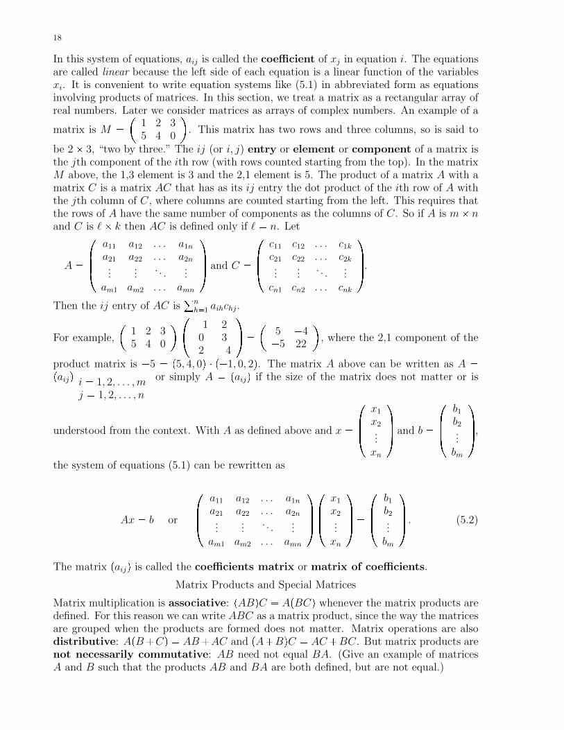
In this system of equations, aij is called the coefficient of xj in equation i. The equationsare called linear because the left side of each equation is a linear function of the variablesxi. It is convenient to write equation systems like (5.1) in abbreviated form as equationsinvolving products of matrices. In this section, we treat a matrix as a rectangular array ofreal numbers. Later we consider matrices as arrays of complex numbers. An example of a

matrix is M ��

1 2 35 4 0

. This matrix has two rows and three columns, so is said to

be 2� 3, “two by three.” The ij (or i, j) entry or element or component of a matrix isthe jth component of the ith row (with rows counted starting from the top). In the matrixM above, the 1,3 element is 3 and the 2,1 element is 5. The product of a matrix A with amatrix C is a matrix AC that has as its ij entry the dot product of the ith row of A withthe jth column of C, where columns are counted starting from the left. This requires thatthe rows of A have the same number of components as the columns of C. So if A is m� nand C is `� k then AC is defined only if ` � n. Let

A �

����

a11 a12 . . . a1n

a21 a22 . . . a2n...

.... . .

...am1 am2 . . . amn

��� and C �

����

c11 c12 . . . c1k

c21 c22 . . . c2k...

.... . .

...cn1 cn2 . . . cnk

��� .

Then the ij entry of AC is°nh�1 aihchj.

For example,

�1 2 35 4 0

�� �1 20 32 �4

� � � 5 �4

�5 22

, where the 2,1 component of the

product matrix is �5 � p5, 4, 0q � p�1, 0, 2q. The matrix A above can be written as A �paijq i � 1, 2, . . . ,m

j � 1, 2, . . . , n

or simply A � paijq if the size of the matrix does not matter or is

understood from the context. With A as defined above and x �

����

x1

x2...xn

��� and b �

����

b1

b2...bm

��� ,

the system of equations (5.1) can be rewritten as

Ax � b or

����

a11 a12 . . . a1n

a21 a22 . . . a2n...

.... . .

...am1 am2 . . . amn

��� ����

x1

x2...xn

��� �

����

b1

b2...bm

��� . (5.2)

The matrix paijq is called the coefficients matrix or matrix of coefficients.

Matrix Products and Special Matrices

Matrix multiplication is associative: pABqC � ApBCq whenever the matrix products aredefined. For this reason we can write ABC as a matrix product, since the way the matricesare grouped when the products are formed does not matter. Matrix operations are alsodistributive: ApB�Cq � AB�AC and pA�BqC � AC�BC. But matrix products arenot necessarily commutative: AB need not equal BA. (Give an example of matricesA and B such that the products AB and BA are both defined, but are not equal.)

19

An m� n matrix is square and of order n if m � n. The transpose of an m� n matrixA is the n � m matrix AT with ij element equal to the ji element of A. The columnsof A are the rows of AT . Note that pAT qT � A. A matrix is symmetric if it equals itstranspose. A symmetric matrix must be square.

Note that the h` element of AB equals the `h element of the matrix BTAT since Bj` isthe `j element of BT and Ahj is the jh element of AT . Therefore, pABqT � BTAT , andrepeating this formula, we obtain

8. pA1A2 � � �AkqT � ATkATk�1 � � �AT2AT1 whenever these matrix products are defined.

The (principal) diagonal of a matrix is the set of ii elements (in row i and columni for some i). These elements are called diagonal, and the other elements of the matrixare called off diagonal. A diagonal matrix is a matrix with every off diagonal elementequal to 0.

The identity matrix of order n, denoted In or simply I, is the n�n diagonal matrix withevery diagonal element equal to 1. For every order n matrix A, AIn � A � InA.

A matrix is upper triangular if every element below the diagonal (every ij element withi ¡ j) equals 0. A matrix is lower triangular if every element above the diagonal (everyij element with j ¡ i) equals 0. A matrix is triangular if it is upper or lower triangular.Usually these terms are restricted to square matrices, but in these notes, there is no reasonto do so.

Solving Linear Equation Systems

In general, the easiest way to find the solutions to a system of linear equations is bysuccessively eliminating variables by adding multiples of some equations to others. Thissection describes a systematic procedure, Gaussian elimination, for doing so.

Consider the equations (5.1), numbered 1 through m, and start with equation 1 andthe first unknown that appears in the equation system (that is, the smallest j such thatakj � 0 for some k). We can ensure that this unknown, xj, appears in the first equationby interchanging the first equation with an equation k in which xj appears. In the newsystem, the coefficient of xj in equation 1 (call it a1j � akj) is nonzero. Then by replacingeach equation i ¡ 1 with the sum of equation i and �aij{a1j times equation 1, we removexj from every equation i ¡ 1. Next we move to the next equation and next unknown thatappears in the system, and perform the same steps. By continuing in this way, we obtain asystem of equations such that whenever an unknown appears in an equation i, it does notappear in any lower equation k ¡ i. The process stops at the final equation. After eachstep, including the last, the set of unknowns satisfying the resulting equations is the sameas the set satisfying the original equations.

It is possible that the final system contains an equation in which 0 is set equal to someother number. In that case, the original equation system has no solution. Otherwise, foreach i, the last equation in which xi appears determines xi as a function of all the xj’s withj ¡ i. From this we can see whether all the xi’s are determined, and if not, how the xi’sthat satisfy all the equations are related to each other. See SB 7.1 for an example of theprocedure described above.

Gaussian elimination can be represented in a simple way by successive multiplication ofthe equations (5.2) by elementary matrices. These matrices are of three types, whichwe call interchanger, adder and multiplier. An interchanger, denoted Eij is a matrixobtained from an identity matrix by interchanging its rows i and j. An adder, denoted

20

Eijprq is a matrix obtained from an identity matrix by adding r times row i to row j (thatis, by replacing row j by the sum of row j and r times row i). A multiplier matrix,denoted Eiprq is obtained from an identity matrix by multiplying its ith row by r � 0.This terminology is justified by the following result.

9. For every n�m matrix A, EijA is the matrix obtained from A by interchanging its rowsi and j. EijprqA is the matrix obtained from A by replacing its row j by its row j plus rtimes its row i. EiprqA is obtained from A by multiplying its row i by r. (Prove this.)

Each step in Gaussian elimination corresponds to replacing the equation system Ax � bby EAx � Eb for some elementary matrix E. The set of solutions x to the first equationsystem is the same as the set of solutions to the second. (Prove this.) The equationsystem Ax � b can be represented a bit more compactly by the m� pn� 1q matrix pA bq,in which the first n columns are the columns of A and the last column is b. Gaussianelimination is then represented by replacing pA bq by an upper triangular matrix F pA bq,where F � FkFk�1 � � �F2F1 and each Fj is an elementary matrix. The matrix F pA bq iscalled a row echelon form of pA bq. To characterize it formally we need more terminology.

We call the first nonzero entry in a row of a matrix a pivot (of that row) and we call thezeros to the left of the pivot in that row leading zeros of that row. (In A, aij is a pivotin row i if it is nonzero and aik � 0 for all k   j. Then each aik with k   j is a leadingzero of row i.) In a row echelon form, each row after the first has more leading zeros thanthe row above it.

To solve the equation system Ax � b, it is convenient to simplify the row echelon formF pA bq � G � pgijq further. For each row i with a pivot gij, we premultiply by Eip1{gijq.In the resulting matrix, the row i pivot equals 1. Next we replace all the elements in thesame column as a pivot and above it by 0. If the pivot is in row i and column j, then thisis accomplished by premultiplying G by Eikp�gkjq for each k   i. The resulting matrix iscalled a reduced row echelon form of pA bq. In such a matrix, every pivot is equal to1, is on or above the diagonal, and is the only nonzero entry in its column. Row echelonforms provide the following characterization of the set of solutions to Ax � b:

10. If a reduced row echelon form of pA bq has a pivot in its last column, then the equationsystem Ax � b has no solution. If the reduced row echelon form has a pivot in each of itsfirst n columns and no pivot in its last column, then the equation system has exactly onesolution x equal to the first n rows of the last column of the reduced row echelon form. Ifthe reduced row echelon form has no pivot in its last column and no pivot in some othercolumn, then the equation system has infinitely many solutions. These are the only possiblecases.

In the last case, in the reduced row echelon form, each equation i with a pivot determinesxi in terms of variables xj with j ¡ i. If row i contains no pivot, then xi is completelyundetermined. It can take any value in R, so there are infinitely many solutions. Note thatin order for the system to have a unique solution, there must be at least as many equationsas unknowns. But this is not sufficient for the solution to be unique.

Result 10 shows that in order for the system to have a unique solution, the reduced rowechelon form of pA bq must have exactly n pivots. The number of pivots in a reduced rowechelon form is the same as the number of pivots in the row echelon form it was obtainedfrom. (Why?) And every row echelon form of a given matrix has the same number ofpivots. (This follows from (10) since the number of solutions of Ax � b depends only onpA bq, not on how it is reduced to row echelon form.) The number of pivots in a row echelonform is important in many contexts, so it has a name.

21

11. The rank of a matrix A, denoted rank A, is the number of pivots in a row echelonform of A.

VERY IMPORTANT: The rank of a matrix is NOT generally the number of pivots in thematrix itself! You have to reduce the matrix before counting the pivots. The discussionabove implies:

12. If A is m� n and E is elementary of order m, then rank EA � rank A ¤ mintm,nu.Result 10 can be restated in terms of the rank.

13. Ax � b has a unique solution if and only if A and pA bq both have rank n. Ax � bhas no solution if and only if rank pA bq is greater than rank A.

Span, Independence and Systems of Equations

Gaussian elimination is a way of solving a system of linear equations, but it does notprovide much intuition about why a solution does or does not exist. Some intuition canbe obtained by interpreting the system geometrically. Let Aj be column j of the matrixA in (5.2). Then Ax � °n

j�1 xjAj. This last expression is a linear combination of the

vectors Aj. The set of linear combinations of a set of vectors tAju is called their span,denoted span tAju. The span of a set of vectors is also called a vector space. A vectorspace is characterized by the property that all linear combinations of elements of the spaceare also in the space. (Prove this.) The span of a nonzero vector can be represented asthe line containing the vector based at the origin. The span of two vectors that are notcollinear is the plane containing those vectors based at the origin. A vector space that iscontained in another vector space V is called a (vector) subspace of V .

The term vector space applies to more general sets of abstract objects that are notnecessarily elements of Rn. A set V is a vector space over R if it contains an element 0and if for every u, v, w P V and s, t P R,a. u� v � v � u,b. pu� vq � w � u� pv � wq,c. v � 0 � v,d. there exists �v P V such that v � p�vq � 0,e. there is a unique element tv in V ; it equals v if t � 1;f. pstqv � sptvq,g. tpu� vq � tu� tv,h. ps� tqv � sv � tv.

The set R in the definition of a vector space is called the set of scalars for the vector space.More generally, the set of scalars could be the set of rationals or complex numbers insteadof R, or more generally any field (this term is defined in books on abstract algebra). Axiomsa. through h. imply that 0v � 0, and that �v is unique and equal to p�1qv. (Prove this.)

Important examples of vector spaces over R that are not subsets of Rn:The set of sequences txtu8t�1 with xt P Rn (each sequence is a vector);The set of functions f : R Ñ Rn (each function is a vector; tf � g is the function withptf � gqpxq � tfpxq � gpxq).

The definition of the span provides a simple necessary and sufficient condition for exis-tence of a solution to an equation system.

22

14. The system Ax � b has at least one solution if and only if b is in the span of thecolumns of A.

Thus the equation system has a solution if and only if b can be expressed as a sum of scalarmultiples of the columns of A. The scalar multiples are just the original column vectorsrescaled, with their directions possibly reversed.

When does the equation system have a unique solution? The discussion of Gaussian elimi-nation showed that there must be at least as many equations as unknowns, so let us assumethat m ¥ n. The existence of multiple solutions is related to a kind of redundancy in theequation system. Some equations do not add restrictions on x beyond those imposed bythe other equations. The characterization in terms of the span provides a geometric inter-pretation for this case too. If one column of A is in the span of the others, then b can bewritten in different ways as linear combinations of different sets of columns of A that havethe same span.

When one vector is in the span of a set of other vectors, we call the entire set of vectorsdependent. A bit more generally, we call a nonempty set of vectors tviuki�1 (linearly)

dependent if there exist scalars λi, not all 0, with°ki�1 λivi � 0. (This allows the set to

contain just one vector, 0.) If the set of vectors is not dependent it is called (linearly)

independent. Thus tviuki�1 is independent if and only if for scalars λi,°ki�1 λivi � 0 ñ

λi � 0, @i. In that case, we also say that the vectors vi themselves are independent. Notethat all the vectors in an independent set are nonzero. (Prove this.)

15. A set of two or more vectors is independent if and only if no one of them is in the spanof the others.

16. If m independent vectors are in the span of k vectors, then m ¤ k.

Proof: Suppose that vectors w1, . . . , wm are independent and in V � spantv1, v2, . . . , vku.Then w1 � 0 and w1 � °

i λivi, for k scalars λi, not all 0. By renumbering the vectorsvi we can assume that λ1 � 0. Therefore, v1 � p1{λ1qw1 �°i¡1pλi{λ1qvi. Any vector in

V can be represented as°ki�1 γivi � pγ1{λ1qw1 �°i¡1rγi � pγ1λi{λ1qsvi, so V is contained

in the span of tw1, v2, . . . , vku (the vectors vi with v1 replaced by w1). It follows thatw2 � θ1w1 �°i¡1 θivi, for some scalars θi, with θj � 0 for some j ¡ 1. (Otherwise w1 andw2 are dependent). Renumbering the vi vectors again, we can let this j be 2. Repeating thesame procedure, we see that V is contained in the span of tw1, w2, v3, . . . , vku, the set of vivectors with v1 and v2 replaced by w1 and w2. If m ¡ k, we continue this way and replaceall k vectors vi so that V is contained in the span of tw1, w2, . . . , wku after renumbering.Then wm is in the span of the other wi vectors, contradicting result 15. So m ¤ k. �

An independent set of vectors is called a basis for the vector space that it spans.

17. Every vector space in Rn other than t0u has a basis. (Prove this.)

18. Let ej P Rn pj � 1, 2, . . . , nq be the n-vector with jth component equal to 1 and everyother component equal to 0. The n vectors ej are independent and span Rn, so they forma basis for Rn. (Prove this.) This basis is called the standard basis for Rn.

19. All bases of a subspace V of Rn have the same cardinality. (Prove this using Result16.) This result extends to vector spaces with infinitely many independent vectors. Thecardinality of a basis of V is called the dimension of V , and is denoted dim V . Thedimension of the space t0u is defined to be 0.

23

20. dim Rn � n. This follows from Result 18.

21. The vectors ej are orthogonal to each other. A set of vectors tviu with this propertypvi � vj � 0, @i, j, i � jq is called orthogonal. If in addition all the vectors have length 1,the set is called orthonormal. The standard basis for Rn is orthonormal.

22. If tviuk�1i�1 is an independent set of vectors and vk � 0 is orthogonal to each vi, i   k,

then tviuki�1 is an independent set.

Proof: Suppose the hypothesis is true and°ki�1 λivi � 0. Then 0 � p°k

i�1 λiviq � vk �λkvk � vk, so λk � 0 and

°k�1i�1 λivi � 0. Since tviuk�1

i�1 is independent, λi � 0, @i   k, so theset tviuki�1 is independent. �

23. Every vector space in Rn other than t0u has an orthonormal basis. The proof showshow to construct one, starting from an arbitrary basis.

Proof: Let taiuki�1 be a basis for V � t0u, a subspace of Rn. We will use induction toconstruct an orthogonal basis tbiu following the Gram-Schmidt process. Let b1 � a1.Now for ` � 1, . . . , k�1, suppose we have an orthogonal basis tb1, b2, . . . , b`u for the span of

ta1, . . . , a`u. Define b`�1 � a`�1 �°`i�1rpa`�1 � biq{pbi � biqsbi. If b`�1 � 0, then a`�1 is in the

span of b1, . . . , b`, which is the span of a1, . . . , a`. But this contradicts the assumption thatthe ai vectors are independent, so b`�1 � 0. Also, b`�1�bj � 0, @j ¤ ` since bi�bj � 0, @i, j ¤ `

and°`i�1rpa`�1 � biq{pbi � biqsbi � bj � a`�1 � bj, @j ¤ `. Therefore tbiuki�1 is an orthogonal basis

of V , and tp1{}bi}qbiuki�1 is an orthonormal basis. �

24. If V is a vector space in Rn and y P Rn then there is a unique v P V such thatpy� vq � x � 0, @x P V . This v is called the (orthogonal) projection of y on V . It is theclosest element to y in V .

Proof: By 23, V has an orthonormal basis tbiuki�1. Define b � y �°ki�1rpy � biq{pbi � biqsbi.

As in the proof of result 23, b � b` � 0, @` ¤ k. By construction, v � y � b P V � span tbiu,and py � vq � x � b � x � 0, @x P V . To show that v is the closest vector to y in V , considerany x P V and let u � x � v. Then y � x � v � b � v � u � b � u and, since u P V , wehave b � u � 0 and py � xq � py � xq � pb� uq � pb� uq � b � b� u � u ¥ b � b, where the weakinequality holds with equality only if u � 0 and x � v. �

25. If the columns of a matrix A are independent, then the equation system Ax � b has atmost one solution x.

Proof: If x and z are distinct solutions, then Ax � Az � b and 0 � Ax�Az � Apx� zq �°λiAi, where λi is the ith component of x � z and Ai is the ith column of A. Not every

λi is 0, so the columns of A are dependent. �

26. An m� n matrix A is called nonsingular if Ax � b has a unique solution x for eachb P Rm. Otherwise the matrix is called singular.

27. A matrix is nonsingular if and only if it is square with all its columns independent.

ñ: If A is nonsingular then its n columns span Rm since every b P Rm is in their span.By Result 16, m ¤ n. Every linear combination of the columns of A can be written as Aλwith λ P Rn. If Aλ � 0 then λ � 0, since the equation Ax � 0 has a unique solution. Thisshows that the n columns of A are independent, so by Result 16, n ¤ m.ð: Under the hypothesis, suppose that there is a vector b P Rm outside the span of thecolumns of A. Then b along with the columns of A form an independent set of n�1 vectors

24

(by Result 15). This contradicts m � n, so there is no such b, and for every b P Rm, Ax � bhas a solution. By Result 25 the solution is unique. �

Square matrices are typically nonsingular. Singularity is the exceptional case. This can beseen from geometric intuition about independent vectors, but we will prove it later.

The discussion in the previous section, in particular, result 13, implies the following.

28. A matrix of order n is nonsingular if and only if its rank is n.

29. Define the column space of a matrix A, denoted ColpAq, to be the span of its columns.Its dimension is the column rank of A, denoted Rank A (with capital R), the maximumnumber of independent columns of A. Define the row space of A, denoted RowpAq, to bethe span of the rows of A. Its dimension is the row rank of A, the maximum number ofindependent rows of A.

30. For every matrix A, dim ColpAq � Rank A.

We will prove that the column and row ranks of any matrix both equal the rank of thematrix. This is useful because it might be easier to count the independent rows or columnsof a matrix than to find the rank by Gaussian elimination. The proof uses some otherdefinitions and results that are important themselves.

31. The kernel of a matrix A (denoted Ker A, and also called nullspace of A) is the setof vectors v with Av � 0. Note that the kernel is a vector space. (Prove this.)

32. Fundamental Theorem of Linear Algebra: If A is m�n, then dim Ker A� Rank A � n.

Proof: Let r � Rank A and k � dim Ker A. Define ej as in Result 18. Let J � t1, . . . , nube such that the set tAjujPJ consists of r independent columns of A. Then Aj � Aej,@j P J . Let tv1, . . . , vku be a basis for Ker A. Let B � tviuki�1 Y tejujPJ . We willshow that B is a basis for Rn, so k � r � n. To show that span B � Rn, considerany w P Rn. Aw is in the span of the columns of A, so there are scalars αj such thatAw � °jPJ αjAej � Ap°j αjejq. Therefore, Apw�°j αjejq � 0 and w�°jPJ αjej P KerA.

So there are scalars δi with w �°jPJ αjej �°i δivi, which implies that w is in the span

of the vectors in B. The vectors in B are independent, since if°ki�1 λivi �

°jPJ γjej � 0

then 0 � Ap°ki�1 λivi �

°jPJ γjejq �

°jPJ γjAj, which implies γj � 0, @j P J . Therefore°k

i�1 λivi � 0 and λi � 0, @i since the vi vectors are independent. �

33. Rank AT � Rank A. (The row and column ranks of A are equal.)

Proof: Let A be m � n with s the maximum number of independent rows. Let tAjujPJbe s independent rows of A. Every other row of A is in the span of these s rows. If therows tAju do not span Rn, then the procedure in the proof of Result 23 shows that thereis a basis for Rn consisting of the s rows tAju along with k additional vectors tv1, . . . , vkuorthogonal to each Aj. Note that s� k � n. Since every row of A is a linear combinationof the Aj vectors, each vi is orthogonal to every row of A. This implies that each vi isin Ker A. Also by construction, every element of Ker A is in the span of the vi vectors.Otherwise it would be possible to add another vi to the list. Therefore k � dim Ker A, sos � n� k � Rank A. �

34. A matrix A is invertible if there is a matrix B such that BA � AB � I, where I isan identity matrix. A matrix B with this property is unique. (Prove this.) It is called theinverse of A and is denoted A�1.

25

35. Every elementary matrix is invertible.

Proof: It is easy to verify that EjiEij � I, Eip1{rqEiprq � EiprqEip1{rq � I and Eijp�rqEijprq �EijprqEijp�rq � I. �

36. A matrix is nonsingular if and only if it is invertible.

Proof ñ: Let A be nonsingular of order n and let ej P Rn be the standard basis vectordefined in Result 18. Let B be the order n matrix with jth column xj, the unique vectorsuch that Axj � ej. The jth column of AB is Axj � ej, so AB � I. Multiplying bothsides by A yields pABqA � IA, so ApBAq � A. Therefore, ApBAqj � Aj, where pBAqjand Aj are the jth columns of BA and A respectively. But the unique solution to Ax � Ajis ej, so pBAqj � ej and BA � I. This shows that B is the inverse of A.Proof ð: Let A be invertible of order n. If Ax � b then A�1b � A�1Ax � x. If x � A�1b,then Ax � AA�1b � b. Therefore Ax � b has a unique solution for each b P Rn, and A isnonsingular. �

Now we prove that the column rank of a matrix equals the number of pivots in its reducedrow echelon form. As a consequence we have

37. For every matrix A, the row rank of A � column rank A � rank A.

Proof: Let G be a reduced row echelon form of A with k pivots and with ith row Gi. Thenrank A � k and the first k rows of G are independent. To see this, suppose that the ijentry of G is a pivot (equal to 1). It is the only nonzero element in column j of G, so if for

some scalars λi we have 0 � °ki�1 λiG

i, then jth component of this last vector is λj � 0.There cannot be more than k independent rows of G since the remaining rows are 0, whichis in the span of every vector. Therefore the row rank of G is k. By result 33, Rank G � k.

Note that for any elementary matrix E, Ax � 0 implies EAx � 0. Also EAx � 0 impliesAx � E�1EAx � E�10 � 0. Therefore, Ker A � Ker EA, and if F is an elementarymatrix, then Ker A � Ker FEA. Repeating this we obtain Ker A � Ker G since G is theproduct of elementary matrices times A. Combining the results above with results 32 and33 we see that the row rank of A equals Rank A � Rank G � k � rank A �

38. rank AB ¤ mintrank A, rank Bu.Proof: Let B be n � ` and let D � AB. Note that ColpDq � ColpAq since every linearcombination of the columns of D equals Dv � ApBvq for some v, and therefore is a linearcombination of the columns of A. So rank D � dim ColpDq ¤ dim ColpAq � rank A. IfBv � 0, then Dv � 0. So Ker B � Ker D and rank D � `� dim Ker D ¤ `� dim KerB � rank B by Result 32. �

39. Let A and B be square. If A and B are nonsingular or if AB is nonsingular thenpABq�1 � B�1A�1.

Proof: If A and B are nonsingular, then pABq�1 � B�1A�1 follows from pB�1A�1qAB �I � ABpB�1A�1q. If AB is nonsingular and A and B are of order n, then AB is of orderand rank n. By Result 38, A and B have rank n and are nonsingular, so, again, theconclusion holds. �

40. If A1A2 � � �Ak is nonsingular for square Ai’s, then pA1A2 � � �Akq�1 � A�1k A�1

k�1 � � �A�12 A�1

1 .

The result follows from repeated application of Result 39.

We sometimes want a single scalar measure of the “size” of a matrix, some sort of averageof the magnitudes of the entries. One possible measure is the Euclidean norm of the row

26

vector formed by listing the rows of the matrix, one after the other. In some contextsanother measure is more convenient:

41. The operator norm of a matrix A is }A} � supt}Ax} : }x} ¤ 1u.

Linear Functions

42. A function f : V Ñ W is called linear if V and W are vector spaces and fpx� tvq �fpxq � tfpvq for all x, v P V and t P R.

Repeated application of this definition proves the next result.

43. If f : V Ñ W is linear, then fp°i λiviq �°i λifpviq for every set of k scalars λi and

k vectors vi P V .

44. Let V � Rn and W � Rm be vector spaces. A function f : V Ñ W is linear if andonly if there is a matrix B such that fpvq � Bv, @v P V .

Proof: The “if” part is easy. (Prove it.) To prove the “only if” part, suppose that f : V ÑW is linear and consider a basis tv1, v2, . . . , vku for V . Each vi is in Rn, so k ¤ n. (Why?)We need to show that there is a matrix B with jth row Bj such that

Bjvi � pfpviqqj for i � 1, . . . , k and j � 1, . . . ,m, (5.3)

where fpviqj is the jth component of the column vector fpviq P Rm. We show that sucha matrix B exists by rewriting (5.3) as vTi B

Tj � fpviqj and in matrix form as ΛBT

j � Fj,

where Λ has vTi as its ith row, and where Fj is a k � 1 vector with ith component fpviqj.The k rows of Λ are independent, so Λ has k independent columns (by Result 33), andthese columns span Rk, by Result 20. Therefore each Fj is in their span, and Bj existssatisfying ΛBj � Fj, for j � 1, . . . ,m. By construction, (5.3) is satisfied, so fpviq � Bvifor i � 1, . . . , k. For each v P V , we have v � °

i λivi for some set of scalars λi, sofpvq � fp°λiviq � °i λifpviq �

°λiBvi � Bv. �

Finally, we use linear algebra to prove the main step in the proof of the first orderconditions necessary for a solution to constrained optimization problems.

Farkas’s Lemma: The system Ax � b, x ¥ 0 has no solution if and only if the systemATy ¥ 0, bTy   0 has a solution (Fang and Puthenpura 1993, p. 60).

45. Theorem of the Alternative: Consider vectors ai P Rn, i � 1, . . . , k, such that V � tv :v � ai   0, @iu is nonempty. If u � v ¤ 0, @v P V , then there are scalars λi ¥ 0 such that

u � °ki�1 λiai.

Partial Proof: We prove the theorem for the case in which the vectors ai are independent.(It can be shown that if they are not and the hypothesis is satisfied then it is also satisfiedfor an independent subset of the vectors, so the conclusion follows from the proof below.)Under the hypothesis, there exists w P V . Let S be the span of the vectors ai and letu � b � c where b is the orthogonal projection of u on S. Then c � ai � 0, @i. For everyε ¡ 0, pc � εwq � ai   0, hence 0 ¥ u � pc � εwq � c � c � εu � w, which implies c � c ¤ 0 and

c � 0. Therefore u � b � °ki�1 λiai for uniquely determined scalars λi.

To show λi ¥ 0, @i, pick an arbitrary aj, let bj be its projection on the span of the other aivectors, and let xj � bj�aj. Then xj �ai � 0, @i � j and xj �aj � xjpbj�xjq � �xj �xj   0.For all ε ¡ 0, pxj � εwq �ai   0, @i, hence 0 ¥ u � pxj � εwq � εu �w�λjaj �xj, which impliesλjaj � xj ¤ 0 and λj ¥ 0, and this is true for all j � 1, . . . , k. �

27

6. Determinants

Determinants can be used to solve systems of equations, compute inverses and test fordefiniteness of matrices; and they have many other uses. The determinant of a squarematrix is a real number, so the determinant can be viewed as function from the set ofsquare matrices to the set of reals. To motivate the definition of the determinant, consider

the equation system Ax � y, where A ��a bc d

. By Result 27 there is a unique solution

x for each vector y P R2 if and only if the columns of A are independent. The columnsof A are independent if and only if ad � bc � 0. (Prove this.) This justifies the term“nonsingular” for an order 2 matrix. The matrix is singular only in the exceptional casewhen ad� bc � 0. We will define the determinant of A above to be���� a b

c d

���� � ad� bc. (6.1)

We will show that a square matrix of any order is nonsingular if and only if its determinantis nonzero. The magnitude of the determinant of the matrix A above equals the area ofthe parallelogram determined by its rows, i.e., the parallelogram with vertices p0, 0q, pa, bq,pc, dq and pa, bq� pc, dq. (Note that it is only the magnitude of the determinant that equalsthe area of the parallelogram. The determinant itself could be negative.) As a special

case, the identity matrix

�1 00 1

has determinant 1, equal to the area of the rectangle

determined by the rows p1, 0q and p0, 1q (the rectangle with vertices p0, 0q, p1, 0q, p0, 1qand p1, 1q). These results also generalize, and the magnitude of the determinant of anorder n matrix is the volume of the parallelopiped determined by its rows. If the rows arev1, v2, . . . , vn, then this parallelopiped is the set of convex combinations of the rows and the0 vector, i.e., the set t°n

i�1 αivi : αi ¥ 0,°αi � 1u.

As the geometric interpretation suggests, if a single row of the matrix is multiplied by ascalar, the area of the corresponding parallelopiped is multiplied by that scalar, so the de-terminant should be multiplied by that scalar. (Check that this is true for the determinantof a 2� 2 matrix defined in (6.1).) More generally, for all a, b, c, d, α, β and t in R,���� a� tα b� tβ

c d

���� ����� a bc d

����� t���� α βc d

���� . (6.2)

(Show that this is correct.) By (6.2), the determinant of an order 2 matrix is a linearfunction of the first row of the matrix, holding the second row fixed. (The second row isthe same in all the matrices in (6.2)). It is easy to check that the determinant is also a linearfunction of the second row of the matrix (holding the first row fixed); so the determinantis a linear function of each row of the matrix separately. It is also a linear function ofeach column separately. This also holds for matrices of any order. The determinant of anidentity matrix is 1, and the determinant of a matrix is 0 if two rows of the matrix areequal. According to Result 60 below, the determinant is the unique function with all theseproperties.

In order to give a formula for the determinant of an arbitrary square matrix, we digressto consider permutations. An n-permutation (also called simply a permutation) is aone-to-one correspondence from a set of integers t1, 2, . . . , nu to itself. Each permutationπ can be denoted by its vector of values: pπp1q, πp2q, . . . , πpnqq. In this notation, there are

28

two 2-permutations, p1, 2q and p2, 1q, and six 3-permutations: p1, 2, 3q, p2, 1, 3q, p1, 3, 2q,p2, 3, 1q, p3, 1, 2q and p3, 2, 1q.X15. Use induction to prove that there are n! � n � pn� 1q � � � 2 � 1 n-permutations.

The identity n-permutation is p1, 2, . . . , nq. Given n-permutations π and µ, the com-position π � µ is also an n-permutation. Each permutation π has a unique inverse π�1

permutation such that π�1 � π is the identity permutation. We will show that every n-permutation can be expressed as a composition of basic permutations that interchange twonumbers and make no other changes. Given j, k P t1, . . . , nu, define the permutation τjkby τjkpjq � k, τjkpkq � j, and τjkpiq � i for i � 1, . . . , n, with i � j, i � k. If j � k,this permutation is called a transposition. τjk, j � k, is a permutation that interchangestwo numbers and makes no other changes: For example, p2, 3, 1q equals the compositionp1, 3, 2q � p2, 1, 3q. (First interchange the first two integers, then interchange the last two.)There are many compositions of transpositions that yield the same permutation: p2, 3, 1qalso equals p3, 2, 1q � p1, 3, 2q.To express an arbitrary permutation π as a composition of transpositions, start with thetransposition π1 � τ1πp1q, which puts πp1q in the first position. Next, in π1, treated asa vector of integers, move πp2q into the second position by applying the transpositionτ2k, where k is the position of πp2q in π1. This defines π2 � τ2k � π1. Now we applya transposition to π2 that interchanges 3 and πp3q, putting πp3q in the third position.Continuing in this way, at the `th stage, we have the permutation π`, a composition oftranspositions, satisfying π`pjq � πpjq for j � 1, . . . , `. Thus, π equals πn, which is acomposition of transpositions.

Every permutation π has a sign, defined as follows. Let αpπq to be the number of in-versions of π, i.e., the pairs pi, jq such that i   j and πpiq ¡ πpjq (the number of pairsof integers whose position gets reversed by π). The sign of π is sign π � p�1qαpπq, alsowritten signpπq. If αpπq is even, then π is called even and its sign is 1. Otherwise, π iscalled odd and its sign is �1.

46. The identity permutation is even. Every transposition is odd. If π is a permutationand τ is a transposition, then τ � π and π have different signs. (Prove these claims.)

It follows from induction that a permutation is even if and only if it is the compositionof an even number of transpositions. More generally,

47. For all n-permutations π and µ, signpπ � µq � psign πqpsign µq. (Why?)

48. Every permutation π has a unique inverse π�1 such that π �π�1 and π�1 �π both equalthe identity permutation. (Prove this.)

Now we can define the determinant of an arbitrary square matrix. Let Πn be the set ofn-permutations and let A � paijq be an order n matrix.

|A| � detA �¸πPΠn

psign πqa1πp1qa2πp2q � � � anπpnq (6.3)

(Check that this formula gives the same definition of the determinant of an order 2 matrixgiven above.) Note that detA is a continuous function of the components of A.

49. detA is a linear function of each row of A, holding the other rows fixed.

Proof: Fix k P t1, . . . , nu. Let B � pbijq satisfy bij � aij whenever i � k. Then B is thematrix obtained from A by replacing its kth row by pbk1, . . . , bknq. Let C � pcijq satisfy

29

cij � aij for i � k, and ckj � akj � tbkj. Then C is obtained from A by replacing the kthrow of A with the sum of that row and t times the kth row of B. The determinant of C is

|C| �¸πPΠn

psignπqrΠi�kaiπpiqspakπpkq � tbkπpkqq

�¸πPΠn

psignπqra1πp1qa2πp2q � � � anπpnq � tpb1πp1q � � � bnπpnqq � |A| � t|B|.�

50. Interchanging two rows of a matrix reverses the sign of the determinant without chang-ing its magnitude: |Ek`A| � �|A|.Proof: Let B � pbijq � Ek`A. Then bkj � a`j, b`j � akj and bij � aij for i, j � 1, . . . , n withi � k, i � `. Given any permutation π, let π � π � τk`. Then signπ � �signπ and bkπpkq �a`,πpkq � a`,πp`q, so b1πp1q � � � bnπpnq � a1πp1q � � � anπpnq and |B| � °πPΠn

psign πqb1πp1q � � � bnπpnq �°πPΠn

p�sign πqakπp2q � � � anπpnq � �|A|. �

51. If two rows of a matrix are equal, then the determinant of the matrix is 0.

Proof: Interchanging the equal rows reverses the sign of the determinant without changingthe matrix or its determinant. So the determinant equals 0. �

52. Adding a multiple of a row to another row of a matrix does not change the determinant:|A| � |Ek`prqA|.Proof: We can treat detA as a function of the rowsAi ofA and write detA � detpA1, . . . , Anq.Then detpA1, . . . , Ak�1, Ak � rA`, Ak�1, . . . , Anq � detA� r detB, where B is formed fromA by replacing the kth row by A`. Since B has two equal rows, its determinant is 0. �

53. |A| � |AT |.Proof: Let AT � pbijq. Then b1πp1q � � � bnπpnq � aπp1q1 � � � aπpnqn � a1π�1p1q � � � anπ�1pnq. Sinceeach permutation has a unique inverse of the same sign, |AT | � °πPΠn

psign πqb1πp1q � � � bnπpnq� °πPΠn

psign π�1qa1π�1p1q � � � anπ�1pnq � |A|. �

It follows that in all statements about determinants above, the terms “row” and “column”can be interchanged.

Next we consider some results that provide ways to compute determinants. The first wayis called “expansion by cofactors.” To define it, we need more notation. Consider an ordern ¥ 2 matrix A � paijq, and let K and L be proper subsets sets of t1, 2, . . . , nu. Define theK, L minor matrix of A to be the matrix ArK;Ls obtained from A by deleting its kthrow and `th column for every k P K and ` P L. For example, if

A �

����

4 3 2 1�1 2 �3 40 �5 6 �21 �4 3 0

��� , then Art2, 3u; t3us �

�4 3 11 �4 0

.

We use the simpler notation Ari, js to denote Artiu; tjus, the ij minor matrix of Aformed by removing the ith row and jth column from A. The determinant of a K,Lor ij minor matrix of A is called a K, L or ij minor of A. The ij cofactor of A isp�1qi�j|Ari, js|.54. Let cij be the ij cofactor of A. For each i � 1, . . . , n, |A| � °n

j�1 aijcij �°nj�1 ajicji.

30

Proof: For every pn � 1q-permutation π there is a unique n-permutation π with πpkq �πpkq, @k   n, and πpnq � n. Then sign π � sign π. If an order n matrix B � pbijq hasbnn as its only nonzero entry in the last row, then |B| � °πPΠn�1

psign πqb1πp1q � � � bnπpnq �bnn°πPΠn�1

psign πqb1πp1q � � � bn�1,πpn�1q � bnn|Brn, ns|. Now suppose that ak` is the onlynonzero entry in row k of A. We can move row k to the last row without changing the orderof the other rows by making n�k successive row interchanges. Then we move column ` of Ainto the last column by making n� ` interchanges. This yields an order n matrix B � pbijqwith Brn, ns � Ark, `s, bnn � ak`, and |A| � p�1q2n�k�`|B| � p�1qk�`bnn|Brn, ns| � ak`ck`,where ck` is the k` cofactor of A. For a general order n matrix A � paijq, |A| � °n

j�1 akjckjsince detA is a linear function of its kth row, and row k of A is

°nj�1 akjej, where ej is the

unit vector with 1 as its jth component. By result 53, |A| � °nj�1 ajkcjk. �

Result 54 allows us to compute the determinant of an order n matrix by reducing it to thesum of terms involving determinants of order n�1 matrices. By repeating the process, theoriginal determinant can be found. This procedure usually involves repeated calculation ofthe same products of matrix components, so it is typically not very efficient for matricesof order 4 or more unless many of the components are zero. A procedure that is typicallymore efficient is to reduce the matrix to row echelon form by multiplying by elementaryinterchangers and adders which do not change the magnitude of the determinant. Thedeterminant of the row echelon form can be evaluated using the following result.

55. The determinant of a triangular matrix is the product of its diagonal components.

Proof: The proposition is true for matrices of order 1. Assume that it is true for everyorder n � 1 matrix and let A � paijq be order n and upper triangular, so that aij � 0 fori ¡ j. By result 54, |A| � °n

j�1 anjcnj � ann|Arn, ns| � annΠn�1i�1 aii, so the proposition is

true for A. �

56. A square matrix is singular if and only if its determinant is zero.

Proof: We showed above that every matrix can be reduced to a triangular row echelonform by multiplying it by elementary interchangers and adders. These multiplications donot change the magnitude of the determinant. The matrix is singular if and only if its rowechelon form has a row with no pivot. By result 55, that is the only case in which thedeterminant of the row echelon form equals 0. �

57. The determinant of the product of two square matrices equals the product of theirdeterminants: |AB| � |A||B|.Proof: If A is singular, then AB is too, by result 38, so |AB| � |A||B| � 0. By results49, 50 and 52, |EB| � |E||B| if E is elementary. Repeated application of this result showsthat it is also true if E is a product of elementary matrices. If A is nonsingular, then itsreduced row echelon form is an identity matrix. In that case, I � EA and A � E�1, whereE and E�1 are products of elementary matrices, so |AB| � |E�1||B| � |A||B|. �

58. The adjoint matrix of A is adj A � CT , where C � pcijq is the matrix of cofactorsof A. If A is nonsingular, then the ij element of A�1 is cji{|A|, so A�1 � p1{|A|qadj A.(Prove this.)

59. Cramer’s Rule: If A is nonsingular and Ax � b, then the jth component of x isxj � |Bj|{|A|, where Bj is the matrix obtained from A by replacing the jth column by b.

31

Proof: Let Ai be the ith column A and let xj be the jth component of x. Let Aipvqbe the matrix obtained from A by replacing its ith column by the vector v. If Ax � b,then b � °n

i�1 xiAi and Ajpbq � pA1 A2 . . . Aj�1

°ni�1 xiAi Aj�1 . . . Anq. Since detA is a

linear function of Ai, |Ajpbq| � °ni�1 xi|AjpAiq|. For each i � j, |AjpAiq| � 0 since two

columns of AjpAiq are equal. So |Ajpbq| � xj|AjpAjq| � xj|A|. If A is nonsingular, thenxj � |Ajpbq|{|A|. �

60. The determinant is the unique function from the set of square matrices to R, with thefollowing properties:

(a) it is multilinear, i.e., linear as a function of each row, holding the other rows fixed,(b) it assigns the value 0 to matrices with two rows that are equal, and(c) it assigns the value 1 to each identity matrix.

Proof: Suppose that a function D has these properties. For any matrix A, DpEijprqAq �DpAq�DpBq � DpAq, whereB is obtained from A by replacing row j by r times row i. Also,DpEiprqAq � rDpAq by (a), andDpEijAq � �DpAq since Eij � Ejp�1qEijp�1qEjip1qEijp�1q.By (c), DpEijprqq � DpIq � 1, DpEiprqq � r and DpEijq � �1. Therefore, DpEq � detpEqand DpEAq � DpEqDpAq if E is elementary. Repeating this shows that these last equa-tions hold also if E is a product of elementary matrices. There is a product of elementarymatrices E such that EA is a reduced row echelon form of A. If EA has a pivot inevery row, then EA � I and DpEAq � detpEAq � 1. If a row of EA has no pivotthen every element of that row is 0 and (a) implies DpEAq � 0 � detpEAq. Therefore,DpAq � DpEAq{DpEq � detpEAq{ detpEq � detpAq. �

7. Basic Topology of Rn and Metric Spaces

The topics in this section are presented in a somewhat different way in SB Chs. 12 and29. The exercises below are based on the notation and terminology of these notes, notof SB. In this section we develop tools needed to formulate and prove the main theoremsof calculus of several variables. Among the tools are definitions of limits, continuity andderivatives, and sufficient conditions for a function to have a maximizer and minimizer.

A central component of many macroeconomic models is the consumption stream of aninfinitely lived “dynasty;” and many models of financial assets include consumption con-tingent on infinitely many possible “states of the world.” In these models, a consumption“vector” is an infinitely long list, or more precisely a function with domain N or Rn. Ana-lyzing the models often requires measuring how far apart the vectors are from each other.To do so we define a “metric space,” generalizing Euclidean space to possibly infinite di-mensions.

A metric space is a set X and a function d : X � X Ñ R� that assigns to each pair ofelements x and y in X a distance dpx, yq from x to y. The function d, called a metric,satisfies for all x, y, z P X,(a) dpx, xq � 0, (b) dpx, yq ¡ 0 if x � y, (c) dpx, yq � dpy, xq (Interpret this) and(d) dpx, zq ¤ dpx, yq � dpy, zq.Property (d) is called the triangle inequality. (Why?) The set X (alone) is often calleda metric space when it is understood what the metric is. Euclidean space is a metric spacewith metric dpx, yq � }x � y}. If X is a metric space with metric d, then every W � Xis a metric space with metric d, restricted to W . Throughout this section, X and Y arearbitrary metric spaces with metrics d and δ respectively, and S and U are subsets of X.

32

The (open) ball of radius r ¡ 0 at x in X is Bxprq � ty P X : dpx, yq   ru, and theclosed ball of radius r ¥ 0 at x in X is ty P X : dpx, yq ¤ ru. S � X is bounded ifit is contained in some ball in X. Otherwise, S is unbounded. We call x P X interiorin S (or an interior point of S) relative to X if it is in an open ball B contained inS. When x is interior in S relative to X, S is called a neighborhood of x relativeto X. (Try drawing pictures to see what these definitions mean.) When it is understoodwhat metric space X is considered, we omit the phrase “relative to X,” as we do in thefollowing definitions. S is open if all of its elements are interior in S. S is closed if itscomplement XzS � tx P X : x R Su is open. We call x a boundary point of S if everyneighborhood of x contains an element of S and an element of XzS. The set of boundarypoints of S is called the boundary of S, denoted BS. The closure of S is the union of Sand the boundary of S and is often denoted S. The definitions of “closed” and “closure”given here are different from the definitions in SB. Exercises below ask you to prove thatthey are equivalent to the definitions in SB.

The terms “open” and “closed” are not opposites. It is possible for a set to be both openand closed, as the following result shows.

61. The empty set H is both open and closed relative to X.

62. The union of any collection of open subsets of X is open. The intersection of finitelymany open subsets of X is open. (Explain why we need the term “finitely many” here.)The intersection of any collection of closed subsets of X is closed. The union of finitelymany closed subsets of X is closed.

Exercises: In problems below, use the definitions above, not those in SB.

X16. Prove result 61.X17. Prove that every open interval is open in R and every closed interval is closed in R.X18. Many sets in Euclidean space are neither open nor closed. Give an example of one.X19. Prove that a set is closed if and only if it contains its boundary.X20. Prove that every closed set that contains S contains the closure of S.X21. Give an example of a collection of closed sets the union of which is not closed.

A sequence in X is a function f : NÑ X, usually denoted txnu8n�1 or txnu, where xn �fpnq. A subsequence of txnu8n�1 is a sequence txkpnqu8n�1, where k is a strictly increasingfunction from N to N. The sequence txnu8n�1 has a limit x if for every neighborhood U of xthere is a number k such that n ¡ k implies xn P U . In that case, we write limnÑ8 xn � x.A sequence cannot have more than one limit. (Prove this.) If x is the limit of txnu8n�1,we say that txnu is convergent or converges and that xn approaches or converges tox as nÑ 8 (n goes to 8). A sequence that does not converge is said to be divergent orto diverge. We call x a cluster point of a set S if every neighborhood of x contains anelement of S other than x. Note the difference between a limit and a cluster point. Theimage of a sequence might have a cluster point even though the sequence has no limit (forexample, xn � p�1qn � p1{nq for n P N). Also, a sequence might have a limit though itsimage has no cluster point (for example xn � x, @n P N).

X22. Explain carefully why each of these examples shows what is claimed.X23. Prove that a set is closed if and only if it contains all of its cluster points.

A cluster point is often called a limit point. But then students sometimes confuse limitsand limit points. A cluster point is also called an accumulation point, as on p. 270 of

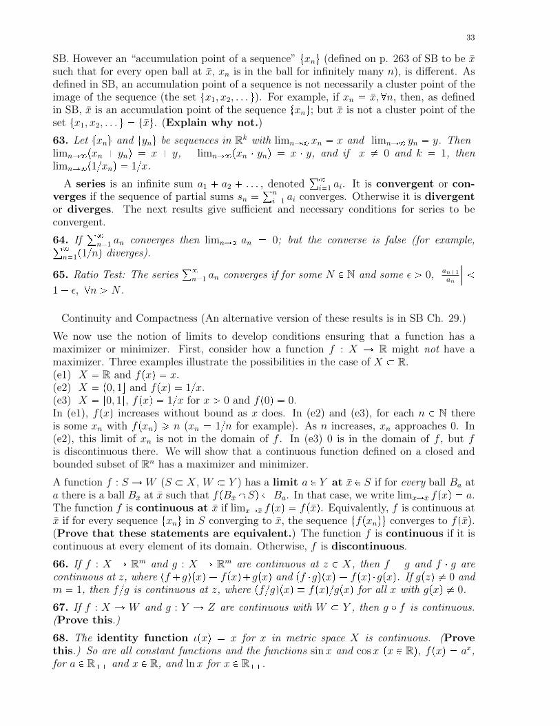
33

SB. However an “accumulation point of a sequence” txnu (defined on p. 263 of SB to be xsuch that for every open ball at x, xn is in the ball for infinitely many n), is different. Asdefined in SB, an accumulation point of a sequence is not necessarily a cluster point of theimage of the sequence (the set tx1, x2, . . . u). For example, if xn � x, @n, then, as definedin SB, x is an accumulation point of the sequence txnu; but x is not a cluster point of theset tx1, x2, . . . u � txu. (Explain why not.)

63. Let txnu and tynu be sequences in Rk with limnÑ8 xn � x and limnÑ8 yn � y. ThenlimnÑ8pxn � ynq � x � y, limnÑ8pxn � ynq � x � y, and if x � 0 and k � 1, thenlimnÑ8p1{xnq � 1{x.

A series is an infinite sum a1 � a2 � . . . , denoted°8i�1 ai. It is convergent or con-

verges if the sequence of partial sums sn � °ni�1 ai converges. Otherwise it is divergent

or diverges. The next results give sufficient and necessary conditions for series to beconvergent.

64. If°8n�1 an converges then limnÑ8 an � 0; but the converse is false (for example,°8

n�1p1{nq diverges).

65. Ratio Test: The series°8n�1 an converges if for some N P N and some ε ¡ 0,

���an�1

an

���  1� ε, @n ¡ N .

Continuity and Compactness (An alternative version of these results is in SB Ch. 29.)

We now use the notion of limits to develop conditions ensuring that a function has amaximizer or minimizer. First, consider how a function f : X Ñ R might not have amaximizer. Three examples illustrate the possibilities in the case of X � R.(e1) X � R and fpxq � x.(e2) X � p0, 1s and fpxq � 1{x.(e3) X � r0, 1s, fpxq � 1{x for x ¡ 0 and fp0q � 0.In (e1), fpxq increases without bound as x does. In (e2) and (e3), for each n P N thereis some xn with fpxnq ¥ n (xn � 1{n for example). As n increases, xn approaches 0. In(e2), this limit of xn is not in the domain of f . In (e3) 0 is in the domain of f , but fis discontinuous there. We will show that a continuous function defined on a closed andbounded subset of Rn has a maximizer and minimizer.

A function f : S Ñ W (S � X, W � Y ) has a limit a P Y at x P S if for every ball Ba ata there is a ball Bx at x such that fpBxXSq � Ba. In that case, we write limxÑx fpxq � a.The function f is continuous at x if limxÑx fpxq � fpxq. Equivalently, f is continuous atx if for every sequence txnu in S converging to x, the sequence tfpxnqu converges to fpxq.(Prove that these statements are equivalent.) The function f is continuous if it iscontinuous at every element of its domain. Otherwise, f is discontinuous.

66. If f : X Ñ Rm and g : X Ñ Rm are continuous at z P X, then f � g and f � g arecontinuous at z, where pf�gqpxq � fpxq�gpxq and pf �gqpxq � fpxq �gpxq. If gpzq � 0 andm � 1, then f{g is continuous at z, where pf{gqpxq � fpxq{gpxq for all x with gpxq � 0.

67. If f : X Ñ W and g : Y Ñ Z are continuous with W � Y , then g � f is continuous.(Prove this.)

68. The identity function ιpxq � x for x in metric space X is continuous. (Provethis.) So are all constant functions and the functions sinx and cosx px P Rq, fpxq � ax,for a P R�� and x P R, and lnx for x P R��.

34

The results above imply that compositions of sums and products of the functions instatement 68 are also continuous. In particular, polynomials are continuous.

Exercises:

X24. Prove that f : X Ñ Y is continuous if and only if for every U � Y open relative toY , the preimage f�1pUq � tx P X : fpxq P Uu is open relative to X.

X25. Define f : R Ñ R with fpxq � 0 for x ¤ 0 and fpxq � x � 2 for x ¡ 0. Is f iscontinuous? Prove that your answer is correct.

A function can be discontinuous even though its graph has no breaks in it. (How?) Also,a function can be continuous even though its graph has breaks in it, as the next exerciseshows. We will discuss this more below.

X26. Prove that g : r0, 1s Y r2, 3s Ñ R is continuous, where gpxq � 0 for 0 ¤ x ¤ 1 andgpxq � x for 2 ¤ x ¤ 3.

X27. Let hp0q � 0 and hpxq � sinp1{xq for x P p0, 1s. Prove that h is discontinuous.

X28. Prove that f : X Ñ Y is continuous if and only if f�1pCq is closed relative to X forevery C � Y closed relative to Y .

In examples (e1) and (e2) above, the function f is continuous but does not have a maxi-mizer. The problem is with the domains. In each case, there is a sequence of elements ofthe domain that does not converge to an element of the domain. This suggests the followingdefinition.

A set X is (limit) compact if every infinite subset of the set has a cluster point in X.We will use this as a definition of a compact set, though “compact” is usually defineddifferently (using open covers). The usual definition is equivalent to the definition givenhere for subsets of metric spaces.

Note that every finite subset of a metric space is compact. (Why?) The set R is notcompact. (Prove this.) Also p0, 1s is not compact. (Prove this.)

69. Every cluster point of a set is the limit of a monotonic sequence in the set and everyneighborhood of the cluster point contains infinitely many elements of the set.

Proof: Let x be a cluster point of S and let B1 be a ball of radius 1 at x. Then B1

contains x1 P S with x1 � x. There is a ball B2 at x with radius }x1 � x}{2   1{2, whichdoes not contain x1, but contains x2 P S with 0   }x2 � x}   1{2. The same way, givenxk�1, we obtain xk P S with 0   }xk � x}   }xk�1 � x}{2   2�k. Then xk convergesto x monotonically and every neighborhood of x contains infinitely many elements of thesequence. �

70. Every sequence in a compact set has a convergent subsequence.

Proof: Let txnu be a sequence in a compact set X. If the set S of points xn is finite,then one of them, say x � xj is repeated infinitely often, so there is an increasing functionm : N Ñ N with xmpnq � x, and the subsequence xmpnq converges to x. If S is infinite,then it has a cluster point x P X. As in the proof of result 69, the ball B1 of radius 1 atx contains some xmp1q and for each k ¡ 1 the ball of radius }xmpk�1q � x}{2 contains somexmpkq � x. Then txmpkqu is a subsequence of txnu that converges to x. �

71. Every bounded closed interval in R is compact.

35

Proof: Let S be an infinite subset of an interval I � ra, bs. We must show that S has acluster point c in I. There will have to be infinitely many elements of S on one side of cand a sequence of points of S converging to c. To find such a c, the idea is to take thehighest number in I with infinitely many larger elements of S. To do this, let W be the setof w P I such that infinitely many elements of S are greater than w. Then a P W and b isan upper bound of W , so W has a least upper bound c P ra, bs. We want to show that c isa cluster point of S. If c   x ¤ b, then x R W , so infinitely many elements of S are belowx. If a ¤ z   c, then z P W , so infinitely many elements of S are above z. This shows thatevery interval pz, xq containing c contains infinitely many elements of S, hence an elementdifferent from c. Thus, c is a cluster point of S. �

72. In a metric space, every finite product of compact sets is compact.

Proof: Let A and B be compact sets in metric space pX, dq. We will prove that A � B iscompact. Then the general case follows by induction. Consider an infinite set S of elementspai, biq of A�B. There must be infinitely many ai’s or infinitely many bi’s. Suppose thereare infinitely many ai’s. (Otherwise interchange the labels a and b.) Then there is asubsequence akpiq converging monotonically to some a P A. If there are infinitely manybkpiq’s, then a subsequence bmpiq of the subsequence bkpiq converges to some b P B. If thereare only finitely many bkpiq’s, then a subsequence of them is constant and equal to someb P B. In either case, pa, bq P A�B is a cluster point of S, so A�B is compact. �

73. paq Every compact subset of a metric space is closed and bounded.pbq If a subset of Euclidean space is closed and bounded, then it is compact.

Proof: (a) Let C be a compact subset of X, a metric space with metric d. If c is a clusterpoint of C, then there is monotonic sequence in C converging to c. This sequence is infiniteand c is its only cluster point, so c is in C since C is compact. This shows that C containseach of its cluster points, so C is closed in X.

Suppose C � X is not bounded. Pick some x0 P X. There exists x1 P C with dpx0, x1q ¡1 and there exists x2 P C with dpx0, x2q ¡ dpx0, x1q � 1 ¡ 2. Continuing in this way, weconstruct an infinite subset S � txnu of C with dpxk, xmq ¡ 1, @k,m P N. The infinite setS has no cluster point. If it had a cluster point x, a ball of radius 1 at x would contain atmost one element of S, but it must contain infinitely many points of S by result 69. Thiscontradiction shows that a compact set C must be bounded.

(b) If C � Rn is bounded, then it is a subset of a product of closed intervals I � I � � � � � Iwith I � R. This product is compact, by results 71 and 72. If C is also closed, then it is aclosed subset of a compact set, hence is compact. �

Some metric spaces contain closed and bounded sets that are not compact. For ex-ample, let X be the set of continuous functions from r0, 1s to r0, 1s and let dpf, gq �maxt|fpxq � gpxq| : 0 ¤ x ¤ 1u. (For a function f P X, fpxq might represent the amountof output produced at date x.)

X29. Prove that this d is a metric for X and that, with this metric, X is bounded andclosed relative to X.

Let S be the set of functions tfnu8n�1 with fnpxq � nx for 0 ¤ x   1{n and fnpxq � 1 for1{n ¤ x ¤ 1.

X30. Prove that X is not compact by proving that S has no cluster point in X.

74. The intersection of a compact set and a closed set is compact. pProve this.q

36

75. Every closed ball in Rn is compact.

Proof: The function fpzq � pz�xq�pz�xq defined on Rn is a sum of products of componentsof z multiplied by constants, therefore is continuous. A closed ball B � tz P Rn : }z�x} ¤ru � f�1pr0, r2sq is the preimage of a closed set, so it is closed. It is bounded by definition,so it is compact. �

76. If f : X Ñ Y is continuous and X is compact, then fpXq is compact.

Proof: Let f be continuous and let X be compact. Suppose that there is an infinite subsetW of fpXq. We need to show that W has a cluster point in fpXq. The idea is to constructan infinite subset S of X in the preimage of W . The subset has a cluster point x in X sinceX is compact, and we show that fpxq is a cluster point of W . But to do this, we need tomake sure that fpSq is infinite.

Consider a sequence of distinct points wn P W . Each wn equals fpxnq for some xn P Xand these xn’s are distinct since f is a function. Since the set of wn’s is infinite, the setof xn’s is infinite and has a cluster point x P X. Let U be any ball at fpxq. Since f iscontinuous, f�1pUq � X is a ball containing x and infinitely many xn’s. For each of thesexn’s, wn � fpxnq P U , and these wn’s are distinct. This proves that fpxq is a cluster pointof W . �

77. If f : X Ñ R is continuous and X compact, then f has a maximizer and a minimizer.

Proof: By Results 73 and 76, fpXq is closed and bounded in R. Therefore it has a supremumy with fpxq ¤ y for all x P X. Every neighborhood of y contains a point y   y, hencecontains fpxq ¡ y for some x P X since y is the least upper bound of fpXq. Therefore y isnot in the complement of fpXq, which is open. So y � fpxq for some x P X, and this x isa maximizer of f . The proof that f has a minimizer is similar. �

A function can have a maximizer even if it is discontinuous and its domain is not compact.

X31. Show that a continuous function f : X Ñ R has a maximizer if and only if there isa compact set S � X and some x P S such that fpxq ¥ fpxq, @x P XzS.

Let tAnu8n�1 be a sequence of subsets of a metric space. The sequence is called nested ifAn�1 � An, @n P N.

78. If tAnu8n�1 is a nested sequence of compact, nonempty sets, then X8n�1An � H.

Connectedness

Next, we formalize the notion of connected sets, which can be used to characterize contin-uous functions and prove the intermediate value theorem. A set S is called disconnectedif it is contained in the union of two disjoint open sets, each having at least one element ofS. Otherwise, S is called connected. Roughly speaking, a disconnected set has separatepieces whereas a connected set does not.

79. If f : X Ñ Y is continuous and S is connected in X, then fpSq is connected in Y .

Proof: Suppose fpSq is disconnected. Then fpSq is contained in the union of two disjointopen sets W and V , each containing at least one element of fpSq. Since f is continuous,f�1pW q and f�1pV q are open sets in X, and each set contains an element of S. AlsoS � f�1pW q Y f�1pV q. And f�1pW q X f�1pV q � H (if not, then there is some x withfpxq P W and fpxq P V , contradicting W X V � H). So S is disconnected if fpSq is. �

Cauchy Sequences, Completeness and the Contraction Fixed Point Theorem

37

We have seen that there are sequences of rationals that converge in the set of reals, buthave no rational limit. We want to be able to say for a metric space whether sequences that“appear to converge” have limits in the space. The sequences are called Cauchy sequences.If they have limits, then the space is called complete.

A sequence txnu in a metric space with metric d is called a Cauchy sequence if for everyε ¡ 0 there exists N P N (depending on ε) such that dpxn, xmq   ε if n ¥ N and m ¥ N .If we follow a Cauchy sequence far enough out, the points of the sequence are all close toeach other. The metric space is complete if every Cauchy sequence in it converges (i.e.,has a limit in the space). An example of a Cauchy sequence in R is txn � 1{nu. (Provethis.) The set S � Rzt0u is a metric space with the metric of the reals dpx, yq � }x � y};but S is not complete since the Cauchy sequence t1{nu does not converge in S. (Its clusterpoint is not in S.)

Exercises:X32. Prove that every convergent sequence in a metric space is a Cauchy sequence.X33. Prove that every Cauchy sequence in a metric space is bounded.X34. Prove that every subsequence of a Cauchy sequence is a Cauchy sequence.X35. Prove that if a subsequence of a Cauchy sequence has a limit then the Cauchysequence has the same limit.X36. Prove that every compact metric space is complete.

80. Every Euclidean space is complete.

This result can be proved using axiom a5 about the set of real numbers (every nonemptyset of reals with an upper bound has a least upper bound).

A function ϕ : X Ñ X is a contraction map (or contraction) of metric space X if thereexists c   1 such that dpϕpxq, ϕpyqq ¤ cdpx, yq, @x, y P X. A contraction of X maps pairsof points in X to pairs of points that are closer together.

X37. Prove that every contraction of a metric space is continuous.

The following fixed point theorem can be used to prove existence of solutions to infinitehorizon optimization problems and to prove the Bellman equation of dynamic programming.We will use it later to prove the Inverse Function Theorem.

81. Contraction Fixed Point Theorem: Every contraction of a complete metric space has aunique fixed point.

Proof: Let X be a complete metric space with metric d, and φ a contraction of X. Pickx0 P X and let xn � φpxn�1q, @n P N. For some c   1, dpxn�1, xnq ¤ cdpxn, xn�1q, @n PN and dpxn�1, xnq ¤ cndpx1, x0q. (Prove by induction.) By the triangle inequality, ifm ¡ n P N, then dpxn, xmq ¤ °m

i�n�1 dpxi, xi�1q ¤ pcn � cn�1 � � � � � cm�1qdpx1, x0q ¤rcn{p1 � cqsdpx1, x0q. This last expression is less than ε ¡ 0 if m ¡ n ¥ N for sufficientlylargeN , since cn Ñ 0 as nÑ 8. Therefore txnu is a Cauchy sequence and converges to somex P X. Since φ is continuous, φpxq � φplimnÑ8 xnq � limnÑ8 φpxnq � limnÑ8 xn�1 � x. Ifx0 is a fixed point of φ, then xn � x0, @n P N, and xn Ñ x implies x0 � x. Since x0 can beany point in X, this proves that x is the unique fixed point of φ. �

8. Functions of Several Variables

Economics considers relations among many variables, so it is important to extend theresults of calculus for functions of a single variable to functions of several variables like

38

F : S Ñ Rm, with S an open subset of Rn. Such a function can be viewed as a list offunctions F � pF iqmi�1 with F i : S Ñ R. The effect of a slight change in the jth argumentof F on the value of F i (per unit change in the argument) is measured by the partialderivative of F i with respect to its jth argument, BF ipxq{Bxj, also denoted BjF ipxqor BxjF ipxq or F i

j pxq. It is the derivative of F ipxq treated as a function of xj with its ith

argument fixed at xi for every i � j. The matrix BF pxq with F ij pxq as its ij element is

called the Jacobian of F at x. A real-valued function of a single variable is differentiableat a point in its domain if it can be well approximated by an affine function near that point.This can be extended in a natural way to a function of several variables.

A function G : Rn Ñ Rm is affine if G�Gp0q is linear, i.e. if there is a matrix A such thatGpxq � Gp0q �Ax, @x P Rn. Then F is differentiable at x P S if it is well approximated byan affine function near x. Formally, F is differentiable at x if there is an affine functionG such that rF pxq �Gpxqs{}x� x} approaches 0 as xÑ x. In that case, for x near x, theapproximation error F pxq �Gpxq is small relative to the distance from x to x. Since thatdistance approaches 0, }F pxq � Gpxq} must too, so F pxq � Gpxq � Gp0q � Ax for somematrix A. Letting v � x � x, it follows that F is differentiable at x if and only if thereis a matrix A such that

limvÑ0

}F px� vq � F pxq � Av}{}v} � 0. (8.1)

(Why?) From this, we see that if F is differentiable at x, then it is continuous at x (Why?)But the converse is false: differentiability is stronger than continuity. Letting xi vary nearxi with xj � xj, @j � i, we can see that the matrix A in (8.1) must be the Jacobianof F at x. (Prove this.) So if F is differentiable at x, then all partial derivatives ofeach F i exist at x. Also, for small v, F px � vq is approximately F pxq � BF pxqv, with anapproximation error that is small relative to the length of v. Existence of the Jacobianmatrix of partial derivatives is not sufficient for F to be differentiable x. The reason isthat the affine approximation to F pxq must be good when two or more components of xvary simultaneously, not just one at a time. For example, the function F : R2 Ñ R, withF pxq � 1 when x " 0 and F px1, x2q � 0 when x1 ¤ 0 or x2 ¤ 0, has the Jacobian matrixBF p0, 0q � p0 0q, but is not continuous at p0, 0q, hence is not differentiable there. It cannotbe approximated by an affine function on the line tpx1, x2q : x1 � x2u. A function F iscalled differentiable if it is differentiable at every element of its domain.

If a real valued function f : S � Rn Ñ R has a (first order) partial derivative functionfipxq � Bfpxq{Bxi that is differentiable, then the second order partial derivatives fijpxq �Bfipxq{Bxj exist for j � 1, . . . , n. If these functions are differentiable, then there are thirdorder partial derivatives fijkpxq � Bfijpxq{Bxk. Similarly, if kth order partial derivativesare differentiable, then their partial derivatives are pk � 1qth order partial derivatives.A function is called C0 if it is continuous, and C0 also denotes the set of continuousfunctions. A function is called Ck or k times continuously differentiable if all of itskth order partial derivatives exist and are continuous. A C1 function is called continuouslydifferentiable. If a function is Ck then it is also C` for each ` � 0, 1, . . . , k. A functionis called C8 if it is Ck for every k P N. The matrix of all second order partial derivativespfijpxqq is called the Hessian matrix of f at x.

82. If a function is continuously differentiable pC1q, then it is differentiable.

The easiest proof of this result uses the mean value theorem proved below. The converseof result 82 is false. There are differentiable functions that are not C1. But most functionsthat appear in economic models are at least piecewise C1. A function f is piecewise

39

C1 if there is a finite partition of its domain tD1, D2, . . . , Dku such that f restricted tothe interior of each Di is C1. Some authors also require a piecewise C1 function to becontinuous.

83. pYoung’s Theoremq If the second order partial derivative fij exists and is continuouson an open ball at x, then the second order partial fji exists and equals fij on that ball. Iff is C2 on a neighborhood of x, then the Hessian matrix of f at x is symmetric.

Affine functions are C8. More complicated C8 functions can be constructed by addingor multiplying such functions together, or by composing such functions.

84. If F and G are Ck functions with the same domain and range, then F �G and F �Gare Ck. If G is scalar valued and nonzero, then F {G is Ck.

85. pChain Ruleq If F : S � Rn Ñ Rm and G : W � Rm Ñ Rk are differentiablerrespectively, C1s with Image F � W , then H � G � F is differentiable rrespectively C1swith Jacobian BHpxq � BGpF pxqqBF pxq at each x P S.

Proof: Let y � F pxq, A � BF pxq , B � BGpF pxqq, φpxq � F pxq � F pxq � Apx � xq,γpyq � Gpyq � Gpyq � Bpy � yq and ψpxq � Hpxq � Hpxq � BApx � xq. We must provethat }ψpxq}{}x� x} Ñ 0 as xÑ x. Note that

ψpxq � GpF pxqq �Gpyq �BApx� xq � γpF pxqq �Bφpxq. (8.2)

Differentiability of F and G at x and y, respectively, implies that for any ε ¡ 0, there existδ ¡ 0 and η ¡ 0 such that }γpyq} ¤ ε}y � y} if }y � y}   η; and }F pxq � F pxq} ¤ η and}φpxq} ¤ ε}x� x} if }x� x}   δ. So }γpF pxqq} ¤ ε}F pxq � F pxq} � ε}φpxq � Apx� xq} ¤ε2}x � x} � ε}Apx � xq} and }Bφpxq} ¤ ε}B}}x � x}. Combining these with (8.2), we seethat }ψpxq} ¤ }γpF pxqq}� }Bφpxq} ¤ ε2}x� x}� ε}A}}px� xq}� ε}B}}x� x}. This showsthat for any ε ¡ 0 there exists δ ¡ 0 such that }ψpxq}{}x � x} ¤ κε if }x � x}   δ, whereκ � ε� }A} � }B}, so }ψpxq}{}x� x} Ñ 0 as xÑ x. �

See SB ch. 14 for examples showing how these theorems are used. Other importantresults concerning functions of several variables can be developed from results on functionsof a single variable.

86. Generalized Mean Value Theorem: If f and g are continuous real valued functions onra, bs that are differentiable on pa, bq, with a   b, then there is some x P pa, bq such thatrfpbq � fpaqsg1pxq � rgpbq � gpaqsf 1pxq.Proof: hptq � rfpbq � fpaqsgptq � rgpbq � gpaqsfptq is differentiable on pa, bq and satisfieshpaq � hpbq. If h is constant on ra, bs then h1pxq � 0 for each x P pa, bq. If h is not constanton ra, bs, then it has a maximizer or a minimizer x in pa, bq at which h1pxq � 0. In eithercase, the equation to be proved holds. �

X38. Prove the Mean Value Theorem: If f : ra, bs Ñ R is a continuous function thatis differentiable on pa, bq, with a   b P R, then there exists x P pa, bq with f 1pxq �rfpbq � fpaqs{pb� aq.87. L’Hopital’s Rule: Let f and g be real valued differentiable functions on pa, bq, with�8 ¤ a   b ¤ 8 and gpxq � 0, @x P pa, bq. Suppose that f 1pxq{g1pxq has a limit as xÑ a.If gpxq Ñ 8 or gpxq Ñ �8 as x Ñ a, or if gpxq Ñ 0 and fpxq Ñ 0 as x Ñ a, thenfpxq{gpxq has the same limit as f 1pxq{g1pxq as xÑ a. The same conclusions hold if xÑ ais replaced by xÑ b.

40

Proof: Let M be an open neighborhood of the limit of f 1pxq{g1pxq as xÑ a. By definition ofthe limit, there is a neighborhood N of a such that for every x, y P N , rfpxq�fpyqs{rgpxq�gpyqs P M since rfpxq � fpyqs{rgpxq � gpyqs � f 1ptq{g1ptq for some t between x and y (byResult 86). If fpyq and gpyq approach 0 as y Ñ a then fpxq{gpxq P M . If gpxq Ñ 8 asxÑ a, then rgpxq� gpyqs{gpxq can be made arbitrarily close to 1 by choosing x sufficientlyclose to a. Holding y fixed and multiplying rfpxq�fpyqs{rgpxq�gpyqs by rgpxq�gpyqs{gpxqwe find that rfpxq � fpyqs{gpxq P M for x sufficiently close to a. But since fpyq{gpxq Ñ 0as xÑ a, fpxq{gpxq PM for x sufficiently close to a. The proof is similar if gpxq Ñ �8 asxÑ a and if xÑ a is replaced by xÑ b. �

Continuous functions with compact domains can be approximated arbitrarily closely bypolynomials. For differentiable functions, a simple approximation is given by Taylor’stheorem. To state the theorem we need more notation. If f : ra, bs Ñ R is differentiable,its derivative f 1 is denoted f p1q. If f 1 is differentiable, its derivative is f2 � f p2q, the second(order) derivative of f . Continuing in this way, the kth (order) derivative of f (if itexists) is f pkq, the derivative of f pk�1q. For n P N, n factorial is n! � npn� 1q � � � 2 � 1 and0 factorial is 0! � 1.

88. Taylor’s Theorem: Let f be a real valued function on ra, bs with f pm�1q continuous onra, bs and f pmq defined on pa, bq for some m P N. If α and x are distinct points of ra, bs,then for some t strictly between α and x,

fpxq � f pmqptqm!

px� αqm �m�1

k�0

f pkqpαqk!

px� αqk (8.3)

Proof: Let pptq � °m�1k�0

f pkqpαqk!

pt�αqk and define µ by fpxq � µpx�αqm�ppxq for the fixed

x in the theorem. Let gptq � fptq � pptq � µpt� αqm for a ¤ t ¤ b. Note that ppmqptq � 0,so gpmqptq � f pmqptq �m!µ. If we show that gpmqptq � 0 for some t between α and x thenf pmqptq � m!µ and (8.3) is proved. Note that gpxq � 0 and that ppjqpαq � f pjqpαq forj � 0, 1, . . . ,m � 1, so gpjqpαq � 0 for j � 0, 1, . . . ,m � 1. By the mean value theorem,g1px1q � 0 for some x1 between α and x, and g2px2q � 0 for some x2 between α and x1.Continuing in this way, we see that gpmqpxmq � 0 for some xm between α and xm�1. �

The polynomial°m�1k�0

f pkqpαqk!

px � αqk is the Taylor series approximation to fpxq at α.According to (8.3), the quality of approximation is better when x is closer to α and whenm is higher, if the derivatives f pmq are bounded on rα, xs.Functions of several variables can be approximated in a similar way. For a real valuedfunction that is Cm in an open subset of Rn, let fi1,i2,...,iq denote the qth order partialderivative of f with respect to its i1, i2, . . . , iqth arguments, with ij P t1, 2, . . . , nu. Theformula below is obtained by applying (8.3) and the chain rule to φptq � fpα � tpx� αqq.89. Multivariable Taylor’s Theorem: Let f be a real valued Cm function on an open setX � Rn. Given α, x P X, let h � phiq � x� α. Then for some t P p0, 1q,

fpxq � fpαq �n

i�1

fipαqhi � 1

2!

n

i,j

fijpαqhihj � � � � � 1

pm� 1q!n

i1,...,im�1

fi1���im�1pαqhi1 � � �him�1

� 1

m!

n

i1,...,im

fi1���impα � thqhi1 � � �him . (8.4)

41

The following result on directional derivatives is an easy application of Taylor’s theorem.A sequence txiu in Rn approaches x from direction v (with }v} � 1) if xi Ñ x andpxi � xq{}xi � x} Ñ v as iÑ 8.

90. If f : X � Rn Ñ R is C1 at x and txiu approaches x from direction v, thenlimiÑ8rfpxiq � fpxqs{}xi � x} � Bfpxqv.

Proof. Under the assumptions, Taylor’s theorem implies fpxiq � fpxq � Bfpxiqpxi � xq foreach i, where xi is an element of the segment joining xi and x. Therefore xi Ñ x andrfpxiq � fpxqs{}xi � x} Ñ Bfpxqv if pxi � xq{}xi � x} Ñ v. �

The Inverse Function Theorem and the Implicit Function Theorem

We have seen that if A is a nonsingular order n matrix then the linear map Apxq �Ax on Rn has a unique inverse. We now show that this result generalizes to nonlinearfunctions, at least locally. The nonlinear generalization of an invertible linear map is calleda diffeomorphism. A one-to-one correspondence from an open set X � Rn to an open setY � Rn is a diffeomorphism if it and its inverse are both C1.

The proof of the Inverse Function Theorem is somewhat difficult and involves the contrac-tion fixed point theorem. We start out with a more limited version of the theorem thatcan be proved more easily.

91. Partial Inverse Function Theorem: If F : X � Rn Ñ Rn is C1 on a neighborhood ofx, with BF pxq nonsingular, then F is one-to-one on a neighborhood of x.

Proof: The determinant |A| is a continuous function of the elements of A, so under thehypotheses of the theorem, there is a neighborhood U of x on which |BF pxq| is continuousand nonzero. Suppose that for every n P N the intersection of U with the ball of radius 1{ncentered at x contains xn and zn (zn � xn) with F pxnq � F pznq. By Taylor’s Theorem,for each n P N there exists wn in the segment joining xn and zn such that F pznq �F pxnq�BF pwnqpzn�xnq, hence BF pwnqpzn�xnq � 0. Let vn � p1{|zn�xn|qpzn�xnq. Thesequence tvnu is contained in the compact sphere of radius 1, therefore has a subsequencetvni

u converging to some v � 0. Since 0 � BF pwniqvni

, @i and wniÑ x and vni

Ñ v,we have BF pxqv � 0, which contradicts |BF pxq| � 0. It follows that some open ball at xcontains no distinct x and z with F pxq � F pzq. So F is one-to-one on this ball at x. �

92. Inverse Function Theorem: If F : X Ñ Rn is C1 with a nonsingular Jacobian matrixBF pxq at x � x, then F restricted to some neighborhood U of x is a diffeomorphism, withinverse G satisfying BGpF pxqq � rBF pxqs�1, @x P U .

The proof will use the result in the following exercise.

X39. Prove that if φ : X Ñ Rn satisfies }Bφpxq} ¤ c, @x P X then }φpxq � φpzq} ¤c}x� z}, @x, z P X.

Proof of Result 92: Let A � BF pxq. Fix y P F pXq. We need to show first that if y issufficiently close to F pxq then there is a unique x with F pxq � y. For this we use a fixedpoint argument. Define φy on X by φypxq � x � A�1py � F pxqq. Note that F pxq � y ifand only if x is a fixed point of φy. Also, Bφypxq � I � A�1BF pxq � A�1pA � BF pxqq and}Bφypxq} ¤ }A�1} � }A � BF pxq}. Since F is C1, the right side of this last equation canbe made arbitrarily small by letting x be sufficiently close to x. Let U be an open ballcentered at x and contained in X, small enough so that the right side of the last inequalityis less than 1/2 and det BF pxq � 0 whenever x P U . By exercise 31,

|φypxq � φypzq| ¤ p1{2q|x� z| for all x, z P U. (8.5)

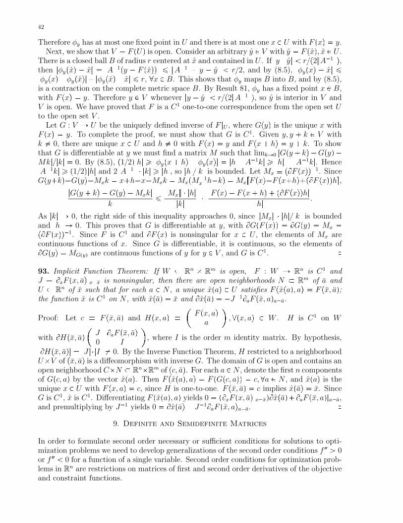
42

Therefore φy has at most one fixed point in U and there is at most one x P U with F pxq � y.Next, we show that V � F pUq is open. Consider an arbitrary y P V with y � F pxq, x P U .

There is a closed ball B of radius r centered at x and contained in U . If |y�y|   r{p2}A�1}q,then |φypxq � x| � |A�1py � F pxqq| ¤ }A�1} � |y � y|   r{2, and by (8.5), |φypxq � x| ¤|φypxq�φypxq|� |φypxq� x| ¤ r, @x P B. This shows that φy maps B into B, and by (8.5),is a contraction on the complete metric space B. By Result 81, φy has a fixed point x P B,with F pxq � y. Therefore y P V whenever |y � y|   r{p2}A�1}q, so y is interior in V andV is open. We have proved that F is a C1 one-to-one correspondence from the open set Uto the open set V .

Let G : V Ñ U be the uniquely defined inverse of F |U , where Gpyq is the unique x withF pxq � y. To complete the proof, we must show that G is C1. Given y, y � k P V withk � 0, there are unique x P U and h � 0 with F pxq � y and F px � hq � y � k. To showthat G is differentiable at y we must find a matrix M such that limkÑ0 |Gpy� kq �Gpyq �Mk|{|k| � 0. By (8.5), p1{2q|h| ¥ |φypx� hq � φypxq| � |h� A�1k| ¥ |h| � |A�1k|. Hence|A�1k| ¥ p1{2q|h| and 2}A�1} � |k| ¥ |h|, so |h|{|k| is bounded. Let Mx � pBF pxqq�1. SinceGpy�kq�Gpyq�Mxk � x�h�x�Mxk �MxpM�1

x h�kq �MxrF pxq�F px�hq�pBF pxqqhs,|Gpy � kq �Gpyq �Mxk|

|k| ¤ }Mx} � |h||k| � |F pxq � F px� hq � pBF pxqqh||h| .

As |k| Ñ 0, the right side of this inequality approaches 0, since }Mx} � |h|{|k| is boundedand |h| Ñ 0. This proves that G is differentiable at y, with BGpF pxqq � BGpyq � Mx �pBF pxqq�1. Since F is C1 and BF pxq is nonsingular for x P U , the elements of Mx arecontinuous functions of x. Since G is differentiable, it is continuous, so the elements ofBGpyq �MGpyq are continuous functions of y for y P V , and G is C1. �

93. Implicit Function Theorem: If W � Rn � Rm is open, F : W Ñ Rn is C1 andJ � BxF px, aq|x�x is nonsingular, then there are open neighborhoods N � Rm of a andU � Rn of x such that for each a P N , a unique xpaq P U satisfies F pxpaq, aq � F px, aq;the function x is C1 on N , with xpaq � x and Bxpaq � �J�1BaF px, aqa�a.

Proof: Let c � F px, aq and Hpx, aq ��F px, aqa

, @px, aq P W . H is C1 on W

with BHpx, aq�J BaF px, aq0 I

, where I is the order m identity matrix. By hypothesis,

|BHpx, aq| � |J | � |I| � 0. By the Inverse Function Theorem, H restricted to a neighborhoodU�V of px, aq is a diffeomorphism with inverse G. The domain of G is open and contains anopen neighborhood C�N � Rn�Rm of pc, aq. For each a P N , denote the first n componentsof Gpc, aq by the vector xpaq. Then F pxpaq, aq � F pGpc, aqq � c, @a P N , and xpaq is theunique x P U with F px, aq � c, since H is one-to-one. F px, aq � c implies xpaq � x. SinceG is C1, x is C1. Differentiating F pxpaq, aq yields 0 � pBxF px, aq|x�xqBxpaq�BaF px, aq|a�a,and premultiplying by J�1 yields 0 � Bxpaq � J�1BaF px, aqa�a. �

9. Definite and Semidefinite Matrices

In order to formulate second order necessary or sufficient conditions for solutions to opti-mization problems we need to develop generalizations of the second order conditions f2 ¡ 0or f2   0 for a function of a single variable. Second order conditions for optimization prob-lems in Rn are restrictions on matrices of first and second order derivatives of the objectiveand constraint functions.

43

Let A � pAijq and B � pBijq be m�n matrices. Then A � B if and only if Aij � Bij fori � 1, . . .m and j � 1, . . . , n. We say that A is at least as great as B and write A ¥ B andB ¤ A if every element of A � B is nonnegative. We say that A is strictly greater than Band write A " B and B ! A if every element of A�B is strictly positive. We say that A issemistrictly greater than B and write A ¡ B and B   A if A ¥ B and A � B. B is callednonnegative [resp. nonpositive] if B ¥ 0 [resp. B ¤ 0]. B is strictly [resp. semistrictly]positive if B " rresp. ¡s0. B is strictly [resp. semistrictly] negative if B ! rresp.  s0.

Let M be a square matrix of order n.

94. M is positive semidefinite [resp. negative semidefinite] on a vector space V � Rn

if xTMx ¥ rresp. ¤s0 for every x P V . M is indefinite on V if it is neither positive nornegative semidefinite on V . We omit reference to V when it is Rn.

95. M is positive definite [resp. negative definite] on V if xTMx ¡ rresp.  s0 forevery nonzero vector x P V . Again we omit reference to V if it is Rn.

Note: Positive definiteness does NOT mean that all the elements of the matrix of thematrix are positive. Similarly, negative definiteness does not mean that all the elementsof the matrix are negative. In math literature, definite and semidefinite matrices are oftenassumed to be symmetric. We will not require definite or semidefinite matrices to besymmetric. The reason is that negative semidefiniteness without symmetry sometimes hasan economic interpretation. For example, the Slutsky matrix of a smooth demand functionis negative semidefinite if and only if the demand function satisfies a weak version of theweak axiom of revealed preference.

To check for definiteness of a matrix M we can study the function QM defined byQMpxq � xTMx. QM is called the quadratic form of M . If M is positive definite thenQMpxq ¡ 0 for each x � 0. If M is symmetric, its definiteness can be checked by examiningthe determinants of certain of its minor matrices. If M is not symmetric, we can studyminor matrices of its symmetric part.

96. The symmetric part of a square matrix M is the matrix �M � p1{2qpM �MT q.97. A square matrix is positive [resp. negative] semidefinite if and only if its symmetricpart is positive [resp. negative] semidefinite. A square matrix is positive [resp. negative]definite if and only if its symmetric part is positive [resp. negative] definite.

98. A principal minor matrix of M is a matrix obtained by deleting a set of rows andthe corresponding columns of M . If the rows with some set of indices are removed then thecolumns with the same indices are removed. The set of indices may be empty, so that norows and columns are removed.

99. A principal minor matrix of M is leading if it is obtained by deleting the last k rowsand columns of M for some k ¥ 0. A principal minor of M is the determinant of aprincipal minor matrix. The principal minor is of order r if the corresponding principalminor matrix is of order r. The principal minor is leading if the corresponding principalminor matrix is leading.

100. For a square matrix M the following three conditions are equivalent:a) M is positive definite.b) Every principal minor of the symmetric part of M is strictly positive.c) Every leading principal minor of the symmetric part of M is strictly positive.

44

Note: The determinant tests b) and c) do not apply to M itself unless M is symmetric.(SYMMETRIZE FIRST, THEN APPLY THE DETERMINANT TEST.) Ac-cording to Result 100, to check if M is positive definite, we do not need to check all theprincipal minors of the symmetric part of M . It is enough to check the leading ones.

101. For an order n matrix M , the following three conditions are equivalent:a) M is negative definite.

b) For r � 1, . . . , n, every order r principal minor of the symmetric part �M has sign p�1qr.c) For r � 1, . . . , n, the order r leading principal minor of �M has sign p�1qr.Again, the DETERMINANT TESTS b) and c) APPLY ONLY TO THE SYMMETRICPART of M . According to Result 101 c), the leading principal minors alternate in sign.The odd order ones are negative and even order ones are positive.

102. A square matrix is positive semidefinite if and only if every principal minor of itssymmetric part is nonnegative.

103. An n�n matrix M is negative semidefinite if and only if for each r ¤ n, every orderr principal minor of the symmetric part of M has sign p�1qr or 0.Thus when M is negative semidefinite, its symmetric part has nonnegative even orderprincipal minors and nonpositive odd order principal minors.

In testing for semidefiniteness, CHECK EVERY PRINCIPAL MINOR, NOT JUST THELEADING ONES. As usual, the determinant tests apply only to the symmetric part of thematrix.

Another test of definiteness or semidefiniteness of a matrix is based on the signs of theeigenvalues of the symmetric part of the matrix. In the next section, we examine eigenvaluesand eigenvectors, which are useful tools for studying linear functions.

Definiteness and Semidefiniteness on Subspaces

Let M be of order n and let A be k � n p1 ¤ k   n). We call B ��

0k A

AT �M

the

symmetric part of M bordered by A. (We write 0k to emphasize that it is an order kmatrix with all elements equal to 0.) A principal minor matrix of B is bordered if itis formed from B by removing rows (and corresponding columns) from among the last n.Given J � t1, 2, . . . , nu, a bordered principal minor matrix of B formed by removing therows and columns with indices in k� J � tk� j : j P Ju is full if ArJ, Js has rank k. Thismeans that after the rows and columns are removed to form the bordered principal minor,the upper border, consisting of k rows has rank k, the highest possible.

As in the case of positive and negative definite matrices, it is not necessary to considerall the principal minors of the relevant matrix. Consider a sequence of principal minormatrices formed from a matrix by starting with the matrix itself, then removing a singlerow and column at a time. The corresponding sequence of principal minors (determinantsof the minor matrices) arranged in order of increasing size of the minor matrices is calleda nested sequence. Formally, a nested minor sequence of a square matrix N startingwith order m is the sequence of principal minors corresponding to the minor matricesNm, Nm�1, . . . , N`, where N` � N and Nj is an order j principal minor matrix of Nj�1 forj � m,m� 1, . . . , `� 1.

104. If M is an order n matrix and A is k � n of rank k, then the following conditionsare equivalent:

45

(a) M is positive definite on Ker A.

(b) Every full bordered principal minor of B (i.e., of �M bordered by A) has sign p�1qk.(c) There is a nested sequence of full bordered principal minors of B starting with order2k � 1, each of sign p�1qk.

105. If M is an order n matrix and A is k � n of rank k, then the following conditionsare equivalent:(a) M is negative definite on Ker A.(b) Every order k �m full bordered principal minor of B has sign p�1qm for

m � k � 1, k � 2, . . . , n.(c) There is a nested sequence of full bordered principal minors of B with order k�m minor

of sign p�1qm, m � k � 1, k � 2, . . . , n.

Thus for M to be negative definite on Ker A, the full bordered principal minors mustalternate in sign depending on the size of the corresponding principal minor matrices. Thesign is 1 or �1 depending on whether an even or odd number of columns of M remain inthe minor matrix. To check for negative or positive definiteness on Ker A it is enough toconsider a single nested sequence of principal minors of the bordered matrix B.

106. M is positive semidefinite on Ker A ô every bordered principal minor of B has signp�1qk or 0.

107. M is negative semidefinite on Ker A ô every bordered principal minor of B of orderk �m has sign p�1qm or 0, m � k � 1, k � 2, . . . , n.

NOTE: ALL CONDITIONS FOR DEFINITENESS AND SEMIDEFINITENESS APPLYTO THE BORDERED MATRIX FORMED WITH THE SYMMETRIC PART OF M .

Hyperplanes, Projections and Convex Sets

A set S � Rn is convex if tx�p1� tqy P S for every x and y in S and every t P r0, 1s. Thismeans that for every pair of points in S, the segment joining them is in S. S is strictlyconvex if for every x and y p� xq in S and every t P p0, 1q, tx� p1� tqy is in the interiorof S. Strictly convex sets are convex sets with curved boundaries.

An important example of a convex set is an affine set (also called a linear manifold). Aset in Rn is affine if it equals x � V � tx � v : v P V u for some x P Rn and subspace V .The vector space V is uniquely determined. (Prove this.) The dimension of the affineset x� V is the dimension of V . A line in R3 is an affine set of dimension 1 and a plane isan affine set of dimension 2. A hyperplane in Rn is a set H � tx P Rn : a � x � bu, where0 � a P Rn and b P R. If x P H, then H � x � V , where V is the vector space orthogonalto a. The hyperplane H is an affine set of dimension n� 1. (Prove these last two claims.)

108. Every affine set is closed and convex. (Prove this.)

109. For every x P Rn and every nonempty set S � Rn with closure S, some y P Sminimizes |x� y| with respect to y P S. Such a y is a closest point in S to x, and |x� y|is called the distance from x to S. In general there may be many closest points in S tox, but there is only one if S is convex.

Proof. Consider arbitrary points x P Rn and z P S. The ball B � tw P Rn : |x�w| ¤ |x�z|uis compact, by Result 75, so B X S is compact. The continuous function fpyq � �px� yq �

46

px�yq restricted to BXS has a maximizer y, which minimizes |x�y| over the same domain.Suppose that S is convex and z is a maximizer of f over B X S. Note that S is convex.Let v � z � y. Then y � tv P B X S for each t P r0, 1s, so φptq � fpy � tvq is maximizedover r0, 1s at 0 and 1. Therefore φ1p0q ¤ 0 and φ1p1q ¥ 0. Since Bfpyq � 2px� yq, we haveφ1ptq � Bfpy� tvq � v � 2px� y� tvq � v, hence, px� yq � v ¤ 0 and px� y� vq � v ¥ 0. Thus,0 ¥ px� yq � v ¥ v � v � |v|2. So v � 0 and y � z, and y is the unique minimizer of |x� y|over B X S. �

Example: Least Squares. Given y P Rn and X, an n � m real matrix, a column vectorXb with b P Rm can be treated as an approximation to y. A least squares approximationis a vector Xb, where b minimizes py � Xbq � py � Xbq with respect to b P Rm. The setof vectors Xb with b P Rm is the vector space V equal to the span of the columns of X.V is closed in Rm. To see this, pick k independent columns of X, where k � rank X,and form a basis for Rm from these columns and additional vectors vi, i � 1, 2, . . . ,m � korthogonal to the k columns of X. This can be done as in the proof of Result 23. ThenV � tx P Rm : vi � x � 0, @i � 1, . . . ,m� ku is the intersection of closed hyperplanes, henceis closed. It follows from Result 109 that a least squares approximation exists. Since V isconvex (prove this) the least squares approximation is unique.

The least squares b maximizes �py �XbqT py �Xbq with respect to b. The necessary first

order condition is 0 � �2py�XbqT BBbpy�Xbq|b�b � 2py�XbqTX � 0, which is equivalent

to XTy � XTXb. The least squares approximation Xb is unique, but this does not meanthat b is unique. If the columns of X are dependent, then infinitely many vectors b yieldthe same least squares approximation Xb. This is called the case of multicollinearity inlinear regression analysis. Alternatively, if the columns of X are independent, then XTXis nonsingular. (If XTXv � 0 for some v � 0 then vTXTXv � pXvq � pXvq � 0, so Xv � 0

and v � 0.) In that case, b is uniquely determined: b � pXTXq�1XTy.

110. For every nonempty set S � Rn the distance function ρpxq from x to S is continuous.

Proof. Let fpz, yq � pz � yq � pz � yq for z, y P Rn, and consider the problem to maximize�fpz, yq subject to pz, yq P Cpxq � txu � S, where S is the closure of S. Since f and thecorrespondence C are continuous, ρpxq, the value function is continuous, by the Theoremof the Maximum (Result 139). �

111. Sets S and Y are said to be separated if there exist p � 0 and c P R such thatps ¥ c ¥ py, @s P S, y P Y .

112. If S � Rn is convex and x P Rn is not in Int S, then txu and S are separated.

Proof. Let S be the closure of S. Suppose that x R S. Let w be the unique closest pointto x in S and let p � x � w � 0. Given an arbitrary z P S, let v � z � w. Then w � tvis in S, @t P r0, 1s, and φptq � px � w � tvq � px � w � tvq is nondecreasing in t, @t P r0, 1s.Therefore, 0 ¤ φ1p0q � �2v � px� wq, so p � v ¤ 0 and p � w ¥ p � z.

If instead x P S, then since x is not an interior point of S, there is a sequence txiu in thecomplement of S converging to x. For each xi there is a unique wi P S that is closest to xiin S. Define pi � p1{|xi � wi|qpxi � wiq. As in the paragraph above, pi � wi ¥ pi � z,@z P S.Since |pi| � 1, @i and since ts P Rn : |s| � 1u is closed and bounded, the sequence tpiu has asubsequence pkn converging to some p � 0, by Result 70. The subsequence twknu convergesto x. (Proof: Given an open ball B of radius r centered at x, there is some m such thatxkn is in the ball of radius r{3 centered at x. Since wkn is the closest point in S to xkn , it

47

cannot be farther from xkn than x is. So wkn P B.) For each z P S, pkn � pwkn � zq ¥ 0converges to p � px� zq, so the limit is nonnegative and p � x ¥ p � z. �

Given S � Rn, the affine hull of S is the set of finite sums°i λixi with xi P S, λi P R, @i

and°i λi � 1. It is denoted ApSq and equals the intersection of all the affine sets containing

S. (Prove this.) The relative interior of S relative to ApSq, denoted ri S, is the setof x P S such that there is an open ball B at x with B XApSq � S. When S is convex, wecall ri S the relative interior of S without referring to the affine hull ApSq.113. If S � Rn is nonempty and convex, then ri S is nonempty and convex, with ri S � S.

Proof. Let S � Rn be nonempty and convex. Its affine hull is ApSq � x0 � V , where Vis a subspace with basis tx1 � x0, . . . , xk � x0u for vectors x0, x1, . . . , xk in S. To show

that ri S is nonempty, consider z � °ki�0 λixi with λi ¡ 0, @i and

°λi � 1. Then z P S

since S is convex, so z � x0 � u for some u P V , and every w P ApSq can be written as

x0� v � z� pv� uq for some v P V . Since v� u P V , it can be written as°ki�1 γipxi� x0q,

so w � z � pv � uq � pλ0 �° γiqx0 �°ki�1pλi � γiqxi. If v � u is in a small enough ball,°

γi   λ0 and γi ¡ �λi, @i ¥ 1, so w is in the convex hull of the vectors xi and in S. Thisshows that there is a ball B at z with B XApSq � S, so z P ri S.

To show that ri S is convex, consider distinct points x P S and z P ri S and anyy � tx � p1 � tqz with t P p0, 1q. There is a ball B at z with B X ApSq � S. Note thatz � r1{p1�tqspy�txq. Replacing y by w near y, we see that fpwq � r1{p1�tqspw�txq is nearz since f is continuous. Thus there is there is a ball B1 at y such that fpwq P B, @w P B1.If w P ApSq, then w � x � v for some v P V , and fpwq � x � r1{p1 � tqsv P ApSq, sofpwq P BXApSq � S. Then, since S is convex, w � tx�p1� tqfpwq P S. This shows thatB1 XApSq � S, so y P ri S and ri S is convex.

To prove ri S � S, note that for each x P S there is a sequence txiu in S converging to x.Since ri S contains some z, the argument in the previous paragraph implies that for eachi, the segment yi P rxi, zs contains yi P ri S with }yi � xi}   1{i. Then yi converges to x,so x P ri S, and the conclusion follows. �

114. Nonempty convex sets S and Y in Rn are separated if and only if (a) or (b) holds:(a) they are contained in the same hyperplane; (b) ri SX ri Y � H.

Proof. ð: Suppose (b) holds. Since 0 R ri S� ri Y , Result 112 implies that some p � 0satisfies 0 ¥ pps � yq, @s P ri S, y P ri Y , hence for all s P S and y P Y . So S and Y areseparated. If (a) holds, then the hyperplane containing S and Y separates them.ñ: Suppose that for some p � 0, ps ¥ py, @s P S, y P Y . If (b) does not hold, then some x isin ri SX ri Y and ps ¥ px ¥ py, @s P S, y P Y . For some ball B at x, z P BXApSq ñ z P S.If some s P S satisfies ps ¡ px, then the segment rs, xs is contained in ApSq, and somez � x in the segment is in B. Then z P ri S and pz ¡ px. Also z1 � x � pz � xq is inB XApSq and satisfies px ¡ pz1. But this contradicts ps ¥ px, @s P S, so no s P S satisfiesps ¡ px. The same argument with the signs reversed rules out ps   px for s P S, sops � px, @s P S. Replacing S by Y in this argument shows that S and Y are contained inthe hyperplane tz : pz � pxu, so (a) holds. �

10. Optimization: Generalization and Proofs

We will consider optimization problems such as a profit seeking firm’s choice of inputs tomaximize w0qpx1, . . . , xnq �°n

i�1wixi, where xi ¥ 0 is the amount of input of good i used,qpx1, . . . , xnq ¥ 0 is the quantity of output produced, and wi ¡ 0 is the price of good

48

i. (Good 0 is the output.) More generally, we consider maximization and minimizationproblems of the form maxxPCpαq fpx, αq or minxPCpαq fpx, αq for f : X � A Ñ R whereCpαq is a nonempty subset of X � Rn for every α P A � Rm. Here, fp�, αq is called theobjective function at α. Its arguments are called control or choice variables, and Cpαqis the constraint set. We are interested not only in the set of maximizing solutions x,but also in the way the set changes in response to changes in the objective function andconstraint set (induced by changes in α).

X40. Show that the profit maximization problem for a firm with a production function fora single output is a special case of the general problem above. What are the variables αand x, the function f and correspondence C?

The solution set for the problem maxxPCpαq fpx, αq is the set of x P Cpαq such thatfpx, αq ¥ fpz, αq, @z P Cpαq. The solution set for minxPCpαq fpx, αq is defined similarly. Anelement of the solution set is called optimal for fp�, αq is in the constraint set. We call x alocal maximizer or a local solution to the maximization problem above if there is aneighborhood N of x relative to X such that x is in the solution set of maxxPCpαqXN fpx, αq.A local minimizer is defined similarly. We restrict attention to problems in which X is anopen subset of Rn and Cpαq is determined by a set of inequality and equality constraints.

It will be convenient to focus on the minimization problem

(P4) min g0px, aq s.t. gipx, aq ¤ bi, i � 1, . . . , k, and hipx, aq � ci, i � 1, . . . ,m,

with gi : X Ñ R and hi : X Ñ R for each i, where X � Rn is open. When g0 � �f ,α � pa, pbiq, pciqq and Cpαq � tx P X : gipx, aq ¤ bi, h

ipx, aq � ci, @iu, problem (P4) isequivalent to the maximization problem above, in the sense that the two problems havethe same solution sets and the same magnitude of the objective function at each solution.

The following theorem gives first order conditions necessary for a solution to (P4) wheneach gi and hi is differentiable on a neighborhood of the solution. The proof uses theseparation theorem in Result 114.

115. Let x be a local solution to (P4). If each hi and each binding gi at x is differentiableat x, then there exist λ � pλ0, λ1, . . . , λkq ¥ 0 and µ � pµ1, . . . , µmq such that the Lagrange

function Lpxq � °ki�0 λig

ipx, aq �°mi�1 µih

ipx, aq satisfies

BLpxq � 0 and λirgipx, aq � bis � 0 for i � 1, . . . , k. (10.1)

We prove the theorem for the case without equality constraints. Each equality constrainthi � ci can then be added by including the inequality constraints hi ¤ ci and �hi ¤ �ci.Proof. Define G � pgiqki�0, W � tpy0, y1, . . . , ykq P Rk�1 : y0   g0pxq, yi ¤ bi, @i � 1, . . . , kuand ψpxq � Gpxq � BGpxqpx � xq. Let B � X be an open ball at x. Then W and ψpBqare convex (prove this) and separated. To show that they are separated, suppose, onthe contrary, that ψpx�q P int W for some x� P B. Then pg0pxq, b1, . . . , bkqT " Gpxq �BGpxqpx� � xq. Define xptq � x � tpx� � xq for t P R. For t near 0, xptq P B andBtGpxptqq|t�0 � BGpxqpx��xq ! pg0pxq, b1, . . . , bkqT�Gpxq � p0, b1�g1pxq, . . . , bk�gkpxqqT .If bj ¡ gjpxq, then the continuity of x and gj imply that gjpxptqq   bj for all t in someball at 0. If bi � gipxq or if i � 0, then Btgipxptqq|t�0   0, so gipxptqq   bi for i ¡ 0 andg0pxptqq   g0pxq when t ¡ 0 is sufficiently near 0. This contradicts the assumption that xsolves (P4). Therefore there is no such x�, and ψpBqX int W � H. Since W has nonemptyinterior, Result 114 implies that W and ψpBq are separated.

49

It follows that some λ � pλiqki�0 � 0 satisfies

λw ¤ λrGpxq � BGpxqpx� xqs, @x P B,w P W. (10.2)

This inequality is violated at x � x if λj   0 and the jth component of w is sufficientlynegative. Therefore λ ¥ 0. Letting x � x and letting w approach pg0pxq, b1, . . . , bkqT in

(10.2) yields λpg0pxq, b1, . . . , bkq ¤ λGpxq, hence°ki�1 λirgipxq� bis ¥ 0 and λirgipxq� bis �

0, i � 1, . . . , k. Then letting w approach the same limit in (10.2) yields λrBGpxqpx� xqs ¥λrpg0pxq, b1, . . . , bkqT � Gpxqs � 0, @x P B. Therefore B°k

i�0 λigipxq|x�x � λTBGpxq � 0

(Prove this last equation), so the first order conditions hold. �

It is possible that λ0 � 0 in (10.1). In that case, the gradient vectors tBgipxquiPI YtBh1pxqumi�1 are dependent, where I the set of binding inequality constraints at x. Thusindependence of those gradient vectors is a constraint qualification, ensuring that the La-grange multiplier λ0 is nonzero.

To see why a constraint qualification is needed to rule out λ0 � 0, consider the problem

max fpx1, x2q � x1 s.t. x2 ¥ 0, and x2 ¤ p1� x1q3,for x1, x2 P R. The constraints imply that p1�x1q3 ¥ 0, so x1 ¤ 1. But x � px1, x2q � p1, 0qis in the constraint set, so it is a solution. The constraints can be written as gi ¤ 0,i � 1, 2, where g1px1, x2q � x2 � p1 � x1q3 and g2px1, x2q � �x2. The gradients of theconstraint functions at x are Bg1pxq � p0, 1q and Bg2pxq � p0,�1q, which are linearlydependent. There are no nonnegative scalars λi satisfying first order condition in Result4: Bfpxq � °λiBgipxq. (Check this.) In the next section, we will consider other constraintqualifications that are often easier to check.

Envelope Theorem

Consider the problem max fpx, aq subject to gipx, aq ¤ bi, i � 1, . . . , k, where f andthe gi functions are C1 on an open set. Let v be the value function for the problem:vpaq � suptfpx, aq : gipx, aq ¤ bi, @iu.When the parameter a, typically the optimal values of the choice variables vary too. Butthe effect on the value function (the optimal value of the objective function) can be found bysimply considering partial derivatives of the objective function f and constraint functionsgi, holding the choice vector fixed at the optimum, x.

116. Suppose that x is a solution to the above problem at a � a, satisfying the necessary firstorder conditions with Lagrange multipliers λi. If v is differentiable at a, and L � f�°i λig

i

is the Lagrange function, then

Bvpaq � BaLpx, aq � Bafpx, aq �¸i

λiBagipx, aq.

In particular, if the binding constraint functions do not vary with a, then Bvpaq � Bafpx, aq.Proof. Consider the auxiliary problem max fpx, aq � vpaq subject to gipx, aq ¤ bi, i �1, . . . , k. Then px, aq is a solution. (Why?) The first order conditions holding a fixed at aare the same as for the original optimization problem. Let λi be the Lagrange multipliers.The first order conditions resulting from differentiation with respect to a are Bafpx, aq �Bvpaq �°i λiBagipx, aq � 0. �

Second Order Conditions

50

Conditions (10.1) are only necessary for a solution to the maximization problem (P4).They may not be sufficient. If more than one element of the constraint set satisfies them,how do we find a solution? It is important to note that some optimization problems do nothave any solution even though they may have points satisfying the first order conditions.If there is a solution to the problem it can be found in many cases by comparing the valueof the objective function at all the points satisfying the necessary first order conditions.But this may be difficult or impossible if we don’t know the parameters, such as p and win the Sample Problem.

We next consider second order conditions necessary for a solution to (P4) and also secondorder conditions which, along with the first order conditions above, are sufficient for a localsolution. We start with necessary conditions for an unconstrained optimum.

117. If x minimizes rresp. maximizess a C2 function f : X Ñ R, where X is open in Rn,then the Hessian matrix B2fpxq is positive semidefinite rresp. negative semidefinites.Proof. Fix v P Rn and let φptq � fpx � tvq. If x minimizes f , then 0 minimizes φ overan open interval. For every t in that interval, Taylor’s theorem implies φp0q ¤ φptq �φp0q � φ1p0qt � p1{2qφ2puqt2 and 0 ¤ φ2puqt2 for some u with |u|   |t|. Continuity of φ2

and the chain rule imply 0 ¤ φ2p0q � v � B2fpxqv. Since this holds for every v P Rn, B2fpxqis positive semidefinite. If x maximizes f , then it minimizes �f , so �B2fpxq is positivesemidefinite and B2fpxq is negative semidefinite. �

For constrained optimization, there is a necessary second order condition only in certaindirections—directions tangent to the boundary of the constraint set or pointing into thatset. The Hessian matrix of the Lagrange function at a solution to (P4) is positive semidefi-nite on the space of vectors orthogonal to the gradients of the equality constraint functionsand the inequality constraint functions with positive Lagrange multipliers.

118. Let x be a local solution to the minimization problem (P4) for given a, b and c.Suppose that each gi and hj is C2 at x and that pλiq, pµiq satisfy the first order conditionsp10.1q with Lpxq � °λig

ipx, aq�°i µihipx, aq and λ0 ¡ 0. Let I � ti ¥ 1 : λi ¡ 0u and let

A be the matrix with rows Bhjpx, aq, j � 1, . . . ,m, and Bgipx, aq for i P I. If the ` � m�#Irows of A are independent (rank A � `), then v � B2Lpxqv ¥ 0 for every v P Ker A withBgipx, aqv ¤ 0 for all binding i. If the vectors Bgipx, aq with gipx, aq � 0 and λi � 0 are

collinear then all the bordered principal minors of

�0 AAT B2Lpxq

have sign p�1q` or 0.

Let B be the p�n matrix with the rows Bhjpx, aq, j � 1, . . . ,m, and Bgipx, aq for all binding

i. If rank B � p, then the bordered principal minors of

�0 BBT B2Lpxq

have sign p�1qp

or 0.

Proof. Fix a and omit it as an argument of each gi and hj. For v P Ker A with v �Bgipxq   0for each binding i R I, consider the equation system gipxq � bi, @i P I, hjpxq � cj, j �1, . . . ,m, and xj � xj � tvj for j � ` � 1, ` � 2, . . . , n, where ` � m � #I. (Assumingthat the rows of A are independent, ` ¤ n.) By the implicit function theorem 93, theequation system has a unique solution xptq for t in a neighborhood of 0, with xp0q � x andBxp0q � v. Since dgipxptqq{dt|t�0 � BgipxqBxp0q   0 for binding i R I, it follows that xptqis in the constraint set for t ¥ 0 near 0. Therefore g0pxptqq ¥ g0pxq. The complementaryslackness conditions imply φptq � Lpxptqq � λ0g

0pxptqq ¥ λ0g0pxq for t ¥ 0 near 0. Since

φ1p0q � 0, we have 0 ¤ φ2p0q � v � B2Lpxqv. The quadratic form on the right side of this

51

last equation is continuous in v, so v � B2Lpxqv ¥ 0, @v P Ker A with Bgipxqv ¤ 0 for eachbinding i. The proof for a local maximizer is the same with g0 replaced by �g0.

By Result 106, the bordered principal minors of

�0 BBT B2Lpxq

have sign 0 or p�1qp if

rank B � p. The same bordered Hessian restriction holds with the vectors Bgipxq removedfrom the border B for all binding i with λi � 0 as long as these vectors are collinear. Thisis because if Bgipxqv ¡ 0 for such i, then replacing v by �v we have Bgipxqv ¤ 0 for allbinding i, so v � B2Lpxqv ¥ 0, @v P Ker A. �

The next result gives a sufficient condition for x to be a strict local minimizer.

119. Let x, λi, i � 0, 1, . . . , k, and µj, j � 1, . . . ,m, satisfy the f.o.c. in Result 115, with

Lpxq � °ki�0 λig

ipx, aq�°mi�1 µjh

jpx, aq, where each gi and hj is C2 at x. If v �B2Lpxqv ¡ 0for every v � 0 with Bgipx, aqv ¤ 0 for all binding i and Bhjpx, aqv � 0, j � 1, . . . ,m,then x is a strict local solution to (P4). This means that there is a ball at x such thatg0px, aq   g0px, aq for every x � x in the ball and the constraint set.

Proof. Fix a and omit it as an argument of each gi and hj. If the conclusion is false,then there is a sequence of vectors v` � 0 converging to 0 as ` Ñ 8 such that for all`, hjpx � v`q � cj, j � 1, . . . ,m, and gipx � v`q ¤ bi, i � 0, 1, . . . , k, where b0 � g0pxq.(Why?) It follows that 0 ¥ Lpx � v`q � Lpxq. By Taylor’s theorem, the right side of thislast inequality equals v` � BLpx`q�p1{2qv` � B2Lpx`qv` for some x` � x� t`v`, with 0   t`   1.Dividing by }v`}2, letting v` � v`{}v`}, we obtain

0 ¥ t`v` � rBLpx`q{pt`}v`}q � p1{2qv` � B2Lpx`qv`. (10.3)

The sequence tt`u is contained in r0, 1s, and tv`u is contained in the closed ball of radius 1,so there is a subsequence `m along which they converge to t and v respectively. Then t`mv`mapproaches 0 from direction v. Since Lpxq � 0, Result 90 implies BLpx`mq{pt`m}v`m}q ÑB2Lpxqv, so by (10.3), 0 ¥ tv � B2Lpxqv � p1{2qv � B2Lpxqv. For each constraint i binding atx, gipx`mq ¤ gipxq, so Result 90 implies Bgipxqv ¤ 0. Similarly Bhjpxqv ¤ 0, @j. This showsthat if x is not a strict local minimizer, then there is some v violating the assumption. �

Convex, Concave, Quasiconvex and Quasiconcave Functions

A function f : Rn Ñ Rm is called nondecreasing [resp. nonincreasing] if for each xand z in Rn, x ¥ z implies fpxq ¥ rresp. ¤sfpzq. (JR use the term increasing for whatwe have called nondecreasing. Their terminology is not standard.) A nondecreasing [resp.nonincreasing] function f � pf 1, . . . , fmq : Rn Ñ Rm is strictly increasing [resp. strictlydecreasing] if for each x and z in Rn and each i � 1, . . . ,m, x " z implies f ipxq ¡ r sf ipzq.The function f is strongly increasing [resp. strongly decreasing] if for each x and zin Rn and each i � 1, . . . ,m, x ¡ z implies f ipxq ¡ r sf ipzq.120. A differentiable function f : S � Rn Ñ R with convex, open domain is nondecreasing[resp. nonincreasing] if and only if Bf ¥ r¤s0. If Bfpxq " rresp. !s0 then f is stronglyincreasing [resp. strongly decreasing].

A function f : S Ñ R defined on a convex set S � Rn is concave [resp. convex] iffor every x and y in S and t P p0, 1q, fptx � p1 � tqyq ¥ r¤stfpxq � p1 � tqfpyq. Thefunction f is strictly concave [resp. strictly convex] if for every x and y p� xq in Sand t P p0, 1q, fptx � p1 � tqyq ¡ r stfpxq � p1 � tqfpyq. The function f is stronglyconcave [resp. strongly convex] if it is C2 and has a negative [resp. positive] definite

52

Hessian matrix B2fpxq for each x P S. The function f : S Ñ R is quasiconcave [resp.strictly quasiconcave] if fptx � p1 � tqyq ¥ r¡smintfpxq, fpyqu for each x and y in Spy � xq and each t P p0, 1q. Note that f is quasiconcave if and only if for each scalar κ theupper contour tx P S : fpxq ¥ κu is convex. JR call the upper contour the superiorset for level κ. The function f : S Ñ R is quasiconvex [resp. strictly quasiconvex] iffptx � p1 � tqyq ¤ r smaxtfpxq, fpyqu for each x and y in S py � xq and each t P p0, 1q.The function f is quasiconvex [resp. strictly quasiconvex] if p�fq is quasiconcave [resp.strictly quasiconcave]. (Prove this.) We check for quasiconvexity or quasiconcavity of afunction by looking at the level sets or upper contours of the function. These are sets in thedomain of the function. To check for convexity or concavity of a function we must look atthe whole graph of the function, which lies in a space of higher dimension than the domain.

NOTE: The terms “concave” and also “quasiconvex” and “quasiconcave” apply only tofunctions, NOT to sets.

Exercises:X41. Prove that if a real valued function f is concave and g : R Ñ R is nondecreasing,then g � f is quasiconcave.X42. Prove that if f : Rn Ñ R is continuous and strictly quasiconcave then for every κ P Rthe set tx : fpxq ¥ κu is strictly convex.X43. Prove: f : S Ñ R is concave ðñ tpx, yq : y ¤ fpxqu is convex.

121. Let S be convex and open in Rn. A C2 function f : S Ñ R is concave [resp. convex]if and only if its Hessian matrix B2fpxq is negative [positive] semidefinite for each x P S.If f is strictly concave [resp. strictly convex] then its Hessian matrix is negative [positive]definite except at “rare points.” The set of rare points has empty interior and contains nosegments. If f is strongly concave [resp. strongly convex] then it is strictly concave [resp.strictly convex] (but the converse is false).

122. (Arrow, Enthoven, Econometrica 1961) Consider problem (P4) without equality con-straints. If each gi, i � 0, 1, . . . , k, is C1 and quasiconvex, then x is a solution if it satisfiesthe constraints and the necessary first order conditions and if one of the following condi-tions holds:(a) Bg0pxq � 0 and g0 is C2 in a neighborhood of x, or(b) g0 is convex.

X44. Prove that problem (P4) has at most one solution if g0 is strictly quasiconvex andthe constraint set is convex.

X45. For each of the following functions, defined on R2�, find the set of points at which the

Hessian matrix exists; compute the Hessian where it exists; then determine whether thefunction is nondecreasing, increasing, strictly increasing, concave, convex, strictly concaveor strictly convex, quasiconcave or quasiconvex, strictly quasiconcave or strictly quasicon-vex. In separate graphs, draw the level set of level 1 for each of the functions in parts b),c) and d).

a) fpx1, x2q � x1{31 xα2 , where α ¡ 0 is a fixed scalar. b) the quadratic form of

�1 04 3

.

c) gpx1, x2q � 3� px1 � 2q2 � px2 � 3q2. d) φpx1, x2q � mintx1, x2{2u.

X46. Show that the intersection of any collection of convex sets is convex.X47. The convex hull of S is the intersection of all the convex sets that contain S.

53

a. Show that a set is convex if and only if it equals its convex hull.b. Show that the convex hull of S equals the set of convex combinations of points in S(i.e., the set of points of the form

°iPI λixi, where I is finite,

°iPI λi � 1 and for each i P I,

λi ¥ 0 and xi P S.)

11. Eigenvalues, Eigenvectors, Diagonalization and Difference Equations

Two matrices A and B are called similar if there is an invertible matrix X such thatX�1AX � B. The matrix A is diagonalizable if it is similar to a diagonal matrix Λ. Inthat case, there is a matrixX such thatX�1AX � Λ, and therefore AX � XX�1AX � XΛand A � XΛX�1.

One reason for wanting to diagonalize a matrix is to simplify the analysis of dynamicmodels. To see why, consider a model in which a firm adjusts its capital stock yt at date ttoward a desired level y� according to the “difference equation” yt � yt�1 � αpy� � yt�1q,t � 1, 2, . . . , with y0 given. The adjustment might not be immediate because it takestime to incorporate new equipment into the production process. The difference equationis called first order since yt depends only on its immediate predecessor yt�1. If yt�1 � y�,then yτ � y� for every τ ¥ t, so y� can be called a steady state or equilibrium value ofthe stock. To analyze the sequence of values yt it is convenient to work instead with theirdeviations zt � yt � y� from the steady state y�. The difference equation can be rewrittenas zt � �y� � yt�1 � αpy� � yt�1q � p1 � αqpyt�1 � y�q or zt � λzt�1, where λ � 1 � α.Starting from any initial value z0, we obtain z1 � λz0, z2 � λz1 � λ2z0 and zt � λtz0. Thestock converges to y� if and only if zt converges to 0 as tÑ 8, and zt converges to 0 if andonly if |λ|   1 (i.e., 0   α   2) or z0 � 0. If z0 � 0 and 0 ¤ λ   1 then yt is closer to y�

than yt�1 is. If λ   0 then there is “overshooting”: zt and zt�1 have opposite signs and thestock yt crosses from one side of y� to the other when t increases.

The above model can be generalized to allow for the simultaneous evolution of severalvariables according to the difference equation

zt � Azt�1, t � 1, 2, . . . ,8, with zt P Rn, z0 given, and A an n� n matrix. (11.1)

The generalization makes it possible to analyze second or higher order difference equations(in which zt depends on zτ , where τ takes more than one value less than t). For example, thedifference equation xt � αxt�1� βxt�2 can be rewritten as (11.1) with zt � pxt, xt�1qT and

A ��α β1 0

. In (11.1), zi,t, the ith component of zt, may depend on a jth component

of zt�1, j � i. But if A is a diagonal matrix with λi as its ii component, then zi,t � λizi,t�1,and the evolution of each component zi,t can be analyzed as in the single variable caseabove.

If A is not diagonal but is diagonalizable, then it is still possible to simplify the analysis.If A � XΛX�1, where Λ is diagonal, then we define Zt � X�1zt and note that Zt �X�1Azt�1 � ΛX�1zt�1 � ΛZt�1. The evolution of each component of Zt can be analyzedseparately as above, and the evolution of zt is determined by zt � XZt. zt converges to 0if Zt converges to 0 as t goes to 8. The stability of the system depends on the magnitudesof the diagonal elements of Λ � X�1AX. The diagonal elements of Λ are eigenvalues of A,and the columns of X are eigenvectors.

Eigenvalues and Eigenvectors, Complex or Real

54

In order to simplify some proofs and allow the largest possible class of matrices to bediagonalizable, in this section, we consider matrices with complex elements. Let C be the setof complex numbers. A complex number has the form x�iy, where x and y are real numbersand i2 � �1. The number x is called the real part of x� iy and the real number y is calledthe imaginary part. The complex number x � iy is real if y � 0, so the set of complexnumbers contains the set of reals. Addition and multiplication of complex numbers can bedefined so that the associative, commutative and distributive rules hold. The product ofa� bi and x� iy is apx� iyq � bipx� iyq � ax� pay � bxqi� byi2 � ax� by � pay � bxqi.The (complex) conjugate of x� iy is x� iy � x� iy. The product of a complex numberz and its conjugate z is a nonnegative real number. (Check this.) We define the norm ormodulus of a complex number z to be |z| � ?zz. Note that |z| � 0 ô z � 0.

123. q � r � q � r and qr � q r. The conjugate of the sum [resp. product] of complexnumbers is the sum [product] of their conjugates.

A complex matrix is a rectangular array of complex numbers. (Note that a special caseof a complex matrix is a real matrix, with every element a real number.) Addition andmultiplication of complex matrices and multiplication by scalars that are complex numberscan be derived from addition and multiplication of the components of the matrices, in thesame way as for real matrices. In this section, all matrices, vectors and scalars are assumedto be complex.

124. An eigenvector (or characteristic vector) of a square matrix A is a vector x � 0satisfying Ax � λx for some complex number λ. The number λ is called an eigenvalue(or characteristic value) of A.

NOTE: We do not call the 0 vector an eigenvector. (Why not?) However, an eigenvaluecan be 0. If x is an eigenvector of A then tx is also an eigenvector for each scalar t � 0.

The next result can be used to compute eigenvalues and eigenvectors.

125. The eigenvalues of an order n matrix A are the values of λ such that |λI � A| � 0.(Prove this.)

The function ppλq � |λI�A| is an n degree polynomial function of λ, called the charac-teristic polynomial of A. It satisfies ppλq � Πn

i�1pλ� λiq, where the λi’s are eigenvaluesof A. (Why?) In this product, the number of terms pλ � λiq with λi � λj for a particularj is called the multiplicity of the eigenvalue λj. The sum of the multiplicities of theeigenvalues of the order n matrix A is n (why?), and the matrix has at most n distincteigenvalues. The characteristic equation of A is |λI � A| � 0.

�

126. The product of the eigenvalues of a square matrix equals the determinant of the matrix.

127. The trace of a square matrix is the sum of its diagonal elements. The trace of amatrix equals the sum of its eigenvalues.

X48. Let A, B, and C be order n real matrices. Prove that trpABCq � trpBCAq. Canthis result be extended to matrices that are not square of the same order?X49. Use 11 to prove 127 for a diagonalizable matrix.

55

Proofs of results 126 and 127: The characteristic polynomial of A � paijq is ppλq � λn �p°i λiqλn�1 � � � � � p�1qnΠiλi � |λI � A|. Substituting λ � 0 in the last equation showsthat p�1qnΠiλi � | � A| � p�1qn|A|. The determinant |λI � A| is a sum of products ofthe entries of λI � A. Among these products are the terms �aiiλn�1, i � 1, . . . , n, andthese are the only terms that include λn�1. (Why?) Thus the coefficient of λn�1 in thepolynomial ppλq is �°i λi and also �°i aii. �

Not every matrix is diagonalizable, but matrices that are not are “rare” in the followingsense. If a matrix is not diagonalizable, then it is the limit of a sequence of diagonalizablematrices, thus it can be approximated arbitrarily closely by a diagonalizable matrix. Theremaining results provide information about which matrices are diagonalizable.

128. Let A be of order n. The following conditions (a), (b) and (c) are equivalent.(a) A is diagonalizable,(b) A has n linearly independent eigenvectors,(c) A � XΛX�1, where Λ is diagonal and the ith column of X is an eigenvector of Acorresponding to eigenvalue Λii, the ii element of Λ, i � 1, . . . , n.

Proof: A is diagonalizable ô A � XΛX�1 ô AX � XΛ for some diagonal matrix Λand some nonsingular matrix X. If the last equation holds, then Axi � Λiixi, where xiis the ith column of X and Λii is the ii element of Λ. In that case, A has n independenteigenvectors xi since X is nonsingular. Conversely, if A has n independent eigenvectorsxi and corresponding eigenvalues Λii, then AX � XΛ where X has ith column xi andΛ � pΛijq is diagonal. �

129. Eigenvectors associated with distinct eigenvalues of a matrix are independent.

Proof: We will use induction on the number k of eigenvectors. The conclusion is true bydefinition for k � 1. Suppose it is true for k � 1 ¥ 1. We need to prove that it is truefor k. Let x1, . . . , xk be eigenvectors of A associated with distinct eigenvalues λ1, . . . , λk.If°ki�1 aixi � 0 for some scalars ai, then multiplying by A yields

°ki�1 aiλixi � 0, and

subtracting λk times the previous equation yields°k�1i�1 aipλi � λkqxi � 0. By hypothesis,

the vectors x1, . . . , xk�1 are independent, so aipλi� λkq � 0 and ai � 0 for i � 1, . . . , k� 1.

Then°ki�1 aixi � 0 implies ak � 0, so the vectors x1, . . . , xk are independent. �

This result along with result 128 implies

130. If the eigenvalues of a square matrix are all distinct, then the matrix is diagonalizable.

131. Eigenvectors associated with distinct eigenvalues of a symmetric matrix are orthogonalto each other.

Proof: Suppose that A is symmetric and Ax � λx and Az � γz. Since λzTx � zTAx �xTAz � γxT z � γzTx, λ � γ implies zTx � 0. �

We will show that symmetric real matrices are diagonalizable, but first we prove a prelim-inary result.

132. If a real matrix has eigenvector x with eigenvalue λ, then it has the conjugate eigen-vector x with eigenvalue λ.

Proof: If A is a real matrix with Ax � λx and x � 0, then Ax � Ax � Ax � λx, so x isan eigenvector of A corresponding to eigenvalue λ. �

133. Every eigenvalue of a symmetric real matrix is real.

56

Proof: Let A be a symmetric real matrix with Ax � λx and x � 0. By Result 132,Ax � λx, so λxT x � xT pλxq � xTAx � pxTAxqT � xTATx � xTAx � xT pλxq � λxTx.Since xTx � xT x � 0, λ � λ, so λ is real. �

A symmetric real order n matrix can have eigenvectors that are not real. However it also hasn independent real eigenvectors that are orthogonal to each other. Define an orthonormalbasis to be an orthogonal basis consisting of vectors of unit length.

134. If A is a symmetric real matrix of order n then A � XΛXT , where the columns of Xare real eigenvectors of A forming an orthonormal basis for Rn, and where Λ is a diagonalmatrix with the eigenvalues of A on its diagonal.

Proof for the case of distinct eigenvalues and sketch of proof for the general case: Let Abe real and symmetric of order n, with Ax � λx and x � v � iw, where v and w are realvectors, not both 0. Then Av� iAw � λv� iλw and Av�λv� ipAw�λwq � 0. By Result133, λ is real, so Av � λv and Aw � λw. Therefore v or w is a real eigenvector associatedwith λ.

Suppose that A has distinct eigenvalues λ1, . . . , λn and corresponding real eigenvectorsx1, . . . , xn orthogonal to each other and nonzero. The eigenvectors are independent, andreplacing each xi by p1{|xi|qxi we obtain an orthonormal basis for Rn consisting of eigen-vectors of A. Let X be the order n matrix with xi as its ith column. Then XTxj � ej, soXTX � I. Since Axi � λixi, AX � XΛ, where Λ is the diagonal matrix with λi as its iicomponent. Therefore, A � XΛXT .

If A does not have distinct eigenvalues, then it is the limit of a sequence of matricestAtu with distinct eigenvalues. Each At equals XT

t ΛtXt with Λt and Xt defined the way Λand X are defined for A above. The matrices Xt and Λt have limit matrices X and Λ as tapproaches 8 and by continuity of matrix multiplication, A � XTΛX. �

A square matrix might not be diagonalizable, but it is similar to a matrix that is nearlydiagonal in the following sense.

135. Every square matrix is similar to a Jordan matrix of the form

J �

������

J1 0 0 . . . 0 00 J2 0 . . . 0 0...

......

. . ....

...0 0 0 . . . Jk�1 00 0 0 . . . 0 Jk

����� , where Ji �

��������

λi 1 0 . . . 0 00 λi 1 . . . 0 00 0 λi . . . 0 0...

......

. . ....

...0 0 0 . . . λi 10 0 0 . . . 0 λi

������� . (11.2)

The diagonal elements of a given submatrix Ji are all equal, and the elements immediatelyabove the diagonal are all ones. The remaining elements are zeros. The numbers λ1, . . . , λkare the distinct eigenvalues of A.

The results on diagonalization above imply the following characterizations of definite andsemidefinite real matrices.

136. A square real matrix is positive rresp. negatives definite if and only if every eigenvalueof its symmetric part is strictly positive rresp. negatives.137. A square real matrix is positive rresp. negatives semidefinite if and only if everyeigenvalue of its symmetric part is nonnegative rresp. nonpositives.

57

Remember to check the eigenvalues of the symmetric part of the matrix (not the eigenvaluesof the matrix itself if the matrix is asymmetric).

More on Difference Equations

The results in the last section make it possible to give a qualitative description of theevolution of solutions to the linear difference equation

yt � Ayt�1 � b, t � 1, 2, . . . , where A is of order n. (11.3)

A steady state of (11.3) is a vector y such that yt�1 � y implies yt � y. There is a uniquesteady state if and only if I � A is nonsingular. (Prove this.) In that case, the steadystate is y � pI�Aq�1b. The stable manifold is the set of y0 such that a solution to (11.3)satisfies limtÑ8 yt � y. If A is diagonalizable, then (11.3) can be solved following the samesteps discussed above. But even if A is not diagonalizable, information about the stabilityof (11.3) can be obtained from the Jordan matrix of A. Let J t be the t-fold product of amatrix J with itself: J t � JJ � � � J (t times).

138. Let A � XJX�1, where J is a Jordan matrix of the form p11.2q with |λi|   1 fori � 1, . . . ,m, and |λi| ¥ 1 for i � m � 1, . . . , n. If y � pI � Aq�1b, then the solution top11.3q is

yt � y �XJ tX�1py0 � yq, t � 1, 2, . . . , and

the stable manifold is the set of vectors y � Xw such that the last n � m components ofw P Rn are 0.

Vectors in the stable manifold are sums of the steady state vector and linear combinationsof eigenvectors corresponding to stable eigenvalues (eigenvalues with modulus less than 1).The steady state y is globally stable if the stable manifold is Rn, in which case everyeigenvalue of A has modulus less than 1. When A has a “unit root,” i.e., an eigenvalue ofmodulus 1, then there are initial values y0 from which solutions to (11.3) do not convergeto the steady state.

We can find explicit solutions to difference equations of the form (11.3) when the vectoryt consists of lagged values of a single real variable. Suppose

xt � a1xt�1 � a2xt�2 � � � � � an�1xt�n�1 � anxt�n � b (11.4)

for xt, aj P R for nonnegative integers t and real aj. The characteristic equation of thecorresponding A matrix is

λn � a1λn�1 � � � � � an�1λ� an � 0. (11.5)

The solutions xt to (11.4) for t ¥ 1 depend on the initial values of xt: x0, x�1, . . . , x1�n. For(11.4) to have a steady state, it is necessary that b � 0 or else that 1�°n

j�1 aj � 0. (Prove

this.) Suppose that the last inequality holds. For each real root λ of (11.5) of multiplicitym, equation (11.4) with b � 0 has solutions λt, tλt, t2λt, . . . , tm�1λt. (Prove this.) Foreach pair of complex roots α � βi of (11.5) of multiplicity m, equation (11.4) with b � 0has solutions rt cospθt � cq, trt cospθt � cq, t2rt cospθt � cq, . . . , tm�1rt cospθt � cq, where

r � |α � βi| � aα2 � β2 and θ P r0, πs. All solutions to (11.4) are linear combinations ofthese solutions and the steady state solution xt � b{p1 �°n

j�1 ajq, @t, where θ and c aredetermined by the initial values of xt.

It is also possible to find explicit solutions to difference equations with varying coeffi-cients. In the first order case,

xt � atxt�1 � bt for t P N, (11.6)

58

we have x1 � a1x0 � b1 and x2 � a2pa1x0 � b1q � b2 � a1a2x0 � a2b1 � b2. Following thispattern, we obtain

xt � x0

t¹j�1

aj ��t�1

j�1

bj

t¹k�j�1

ak

� bt, for t P N, (11.7)

which can be proved by induction.

12. Miscellaneous

Comparative Statics

We wish to consider optimization problems in which the constraint set varies depending oncertain parameters. We will state conditions (weaker than those appearing in the implicitfunction theorem) under which the optimal choice variables and/or the optimal value ofthe objective function vary continuously as functions of the parameters.

A correspondence from S to Y is a map that assigns to each element of S a subset ofY . The correspondence C from S to Y is upper hemicontinuous if its graph tps, yq :y P Cpsqu is closed and the image CpBq � YsPBCpsq of each nonempty compact set B � Sis nonempty and compact. C is lower hemicontinuous if for each s P S, each y P Cpsqand each sequence tsiu converging to s, there is a sequence yi P Cpsiq converging to y. Cis continuous if it is upper hemicontinuous and lower hemicontinuous.

139. Theorem of the Maximum: If C is a continuous correspondence from S to Y andf : Y Ñ R is continuous, then the solution correspondence ξ (where ξpsq is the set ofmaximizers of f over Cpsq), is upper hemicontinuous and the value function v (where vpsqis the maximum value of f over Cpsq) is continuous.

Proof: Consider a sequence tpsi, yiqu in S � Y converging to ps, yq. If yi P ξpsiq, @i, theny P Cpsq since the graph of C is closed. It follows that vpsiq � fpyiq, @i and that vpsq ¥ fpyq.Also, fpyq � limiÑ8 vpsiq since f is continuous. If fpyq ¡ fpyq for some y P Cpsq then sinceC is lower hemicontinuous, there is a sequence zi converging to y with zi P Cpsiq, @i. Sincef is continuous, fpziq converges to fpyq, which contradicts fpziq ¤ vpsiq, @i. Thereforefpyq ¤ fpyq, @y P Cpsq and y P ξpsq, so the graph of ξ is closed. Also vpsiq Ñ vpsq, so v iscontinuous.

To complete the proof that ξ is upper hemicontinuous, consider a nonempty compactsubset B of S. Let W be an infinite subset of ξpBq. Since W � CpBq and C is upperhemicontinuous, W has a cluster point w in CpBq. There is a sequence twiu inW convergingto w and the proof in the paragraph above, with yi replaced by wi shows that w P ξpsq forsome s P S. Therefore ξpBq is compact and nonempty, and ξ is upper hemicontinuous. �

Three Fixed Point Theorems

A fixed point of a function f : X Ñ X is a point x P X with fpxq � x.

140. Brouwer Theorem: f : X Ñ X has a fixed point if it is continuous and X is nonempty,compact and convex.

141. Kakutani Theorem: Let X � Rn be compact and convex. If C is an upper hemicon-tinuous correspondence assigning to each element of X a nonempty convex subset of X,then there exists x with x P Cpxq.

59

142. Tarsky Theorem: Given a ¤ b P R, if f : ra, bsn Ñ ra, bsn is nondecreasing, then ithas a fixed point.

Exponential and Logarithmic Functions

We now use the results from the previous sections to define the functions lnx and bx forb ¡ 0, and prove that they are the functions we are already familiar with. In particular,they are differentiable and satisfy dplnxq{dx � 1{x and dpbxq{dx � bxpln bq. We also definethe number e and prove e � limnÑ8p1� p1{nqqn, ln e � 1 and dpexq{dx � ex.

We start by defining the function Epxq � °8n�0 x

n{n! for x P R. Then E is well definedsince 0! � 1, and the series in the definition converges (by the ratio test). Note thatEp0q � 1 since 00 � 1.

143. Epx� yq � EpxqEpyq, @x, y P R.

Proof.

EpxqEpyq �8

n�0

xn{n!8

m�0

ym{m! �8

n�0

n

k�0

xkyn�k{rk!pn� kq!s

�8

n�0

p1{n!qn

k�0

�n

k

xkyn�k �

8

n�0

px� yqn{n! � Epx� yq.

�

144. E is differentiable, with E 1 � E.

It is tempting to try to prove this by noting that dpxn{n!q{dx � xn�1{pn � 1q! for eachn ¥ 1 and that

°8n�1 x

n�1{pn� 1q! � Epxq. But this is not a proof. (Why not?)

Proof. For h P Rzt0u,

rEphq � 1s{h � p1{hq8

n�1

hn{n! �8

n�1

hn�1{n! � 1�8

k�1

hk{pk � 1q!

and limhÑ0rEphq � 1s{h � 1. So

E 1pxq � limhÑ0rEpx� hq � Epxqs{h � lim

hÑ0EpxqrEphq � 1s{h � Epxq.

�

145. E ¡ 0.

Proof. By definition, Epxq ¡ 0 for x ¡ 0. If Epxq ¤ 0 for some x, then a � suptx :Epxq ¤ 0u is finite, and continuity of E implies Epaq � 0 � EpaqEp�aq � Ep0q � 1, acontradiction. So Epxq ¡ 0, @x. �

146. If F : R Ñ R satisfies F 1 � F , then for some c, F pxq � cEpxq, @x. E is the uniquefunction with E 1 � E and Ep0q � 1.

Proof. Define fpxq � F pxq{Epxq. Then fpxqEpxq � F pxq � F 1pxq � f 1pxqEpxq �fpxqE 1pxq � pf 1pxq � fpxqqEpxq, so f 1 � 0 and f � c for some c P R. If F p0q � 1,then c � 1. �

147. E has an inverse function defined on R�� and denoted ln, satisfying lnpxyq � lnx�ln y and dplnxq{dx � 1{x, @x ¡ 0.

60

Proof. By definition, Epxq ¡ x for x � 0, so the image of E is unbounded above. Since1{Epxq � Ep�xq, E is not bounded above 0. Therefore every a ¡ 0 satisfies a � Epxq forsome x, denoted ln a. Given a, b P R��, with a � Epxq and b � Epyq, we have ln ab �lnEpx � yq � x � y � ln a � ln b. Let gpxq � lnx for x ¡ 0. Since Epgpxqq � x, @x ¡ 0,E 1pgpxqqg1pxq � 1 and g1pxq � 1{E 1pgpxqq � 1{Epgpxqq � 1{x. �

148. We define e � Ep1q � °8n�0 1{n! and bx � Eppln bqxq for b ¡ 0, x P R.

X50. Prove that fpxq � bx and its inverse function logb x have properties E1 through E4and L1 through L4 in section 2.

149. e � limnÑ8p1� 1nqn

Proof: For n ¡ 0, lnp1 � p1{nqqn � n lnp1 � p1{nqq � p1{xq lnp1 � xq, where x � 1{n.Therefore, using L’Hopital’s Rule, limnÑ8rlnp1 � p1{nqqns � limxÑ0p1{xq lnp1 � xq �limxÑ0r1{p1 � xqs � 1. Since ey is continuous in y, e � e1 � elimnÑ8rlnp1�p1{nqqns �limnÑ8 e

lnp1�p1{nqqn � limnÑ8p1� p1{nqqn. �

150. Limits of CES Functions: Given xi ¡ 0, αi ¡ 0, i � 1, 2, with α1 � α2 � 1,

limρÑ0pα1x

ρ1 � α2x

ρ2q1{ρ � xα1

1 xα22 , and lim

ρÑ�8pα1x

ρ1 � α2x

ρ2q1{ρ � mintx1, x2u.

Proof: Let φpρq � lnrpα1xρ1 � α2x

ρ2q1{ρs � p1{ρq lnpα1x

ρ1 � α2x

ρ2q. By L’Hopital’s Rule,

limρÑ0 φpρq equals

limρÑ0

dpα1xρ1 � α2x

ρ2q{dρ

α1xρ1 � α2x

ρ2

� limρÑ0

α1xρ1plnx1q � α2x

ρ2plnx2q

α1 � α2

� α1plnx1q � α2plnx2q.So limρÑ0 exptlnrpα1x

ρ1 � α2x

ρ2q1{ρsu � exprlimρÑ0 φpρqs � exprα1plnx1q � α2plnx2qs �

xα11 x

α22 . Also,

limρÑ�8

φpρq � limρÑ�8

α1xρ1plnx1q � α2x

ρ2plnx2q

α1xρ1 � α2x

ρ2

� limρÑ�8

α1plnx1qpx1{x2qρ � α2 lnx2

α1px1{x2qρ � α2

.

This limit equals ln x1 if x1 ¤ x2, and equals lnx2 if x1 ¡ x2. So limρÑ�8 exprφpρqs �exprlimρÑ�8 φpρqs equals x1 if x1 ¤ x2 and equals x2 otherwise. �