ece team report - field robotics centerfrc.ri.cmu.edu/~dk683/dongki/research/data/final ece...
TRANSCRIPT

Michael Grisanti • Alicia Violeta Juarez Crow Andrew Doberstein • Prathika Gopalkrishna • Randeep Grewal
Abdurrahman Husnein • Rahul Jain • Anusha (Tess) Jain • Dong Ki Kim Syed Tahmid Mahbub • Jin Sha • Tejaswini Srinivasa • Will (Shunyao) Pan
Richard Quan • Richard Speranza • Tyler Walker • Shela Wang Andrew Chien • Justin Kerber • Kevin Lin • Crystal Lu
ECE TEAM REPORT | CORNELL CUP USA PRESENTED BY INTEL | ACADEMIC ADVISOR: DR. DAVID SCHNEIDER
ECE Team Report CORNELL CUP USA PRESENTED BY INTEL
2013-2014

ECE Team Report 05/18/2014
CORNELL CUP USA PRESENTED BY INTEL Page 2 of 182 2013-2014
Table of Contents Table of Figures ............................................................................................................................................. 6
Table of Tables .............................................................................................................................................. 9
1 Project Overview ................................................................................................................................. 10
General Overview ....................................................................................................................... 10
Division of Labor ......................................................................................................................... 10
1.2.1 Mechanical Engineering Team ............................................................................................ 11
1.2.2 Computer Science Team ..................................................................................................... 11
1.2.3 Electrical and Computer Engineering Team ........................................................................ 11
System Design ............................................................................................................................. 12
1.3.1 Context Diagram ................................................................................................................. 12
1.3.2 Timeline ............................................................................................................................... 14
2 FPGA Development Board Design ....................................................................................................... 14
Introduction ................................................................................................................................ 14
2.1.1 Selected FPGA Development Board .................................................................................... 15
2.1.2 Additional DE2i-150 Documentation and Resources .......................................................... 16
Setting up the FPGA Board.......................................................................................................... 16
2.2.1 Install Required Development Software ............................................................................. 16
2.2.2 Power On and Connect the FPGA ....................................................................................... 19
2.2.3 Programming the FPGA ....................................................................................................... 19
2.2.4 Installing Windows 7 ........................................................................................................... 20
2.2.5 Starting New Project ........................................................................................................... 22
2.2.6 Editing Code ........................................................................................................................ 22
2.2.7 Example Program ................................................................................................................ 22
Pulse Width Modulation ............................................................................................................. 23
2.3.1 PWM Input .......................................................................................................................... 23
2.3.2 PWM Output ....................................................................................................................... 26
2.3.3 Creating the Verilog Program ............................................................................................. 28
Matrix Multiplication using FPGA ............................................................................................... 28
2.4.1 Design .................................................................................................................................. 28
2.4.2 Testing Strategy .................................................................................................................. 29
Intel Atom Communication ......................................................................................................... 30
2.5.1 PCI Communication Setup .................................................................................................. 30
2.5.2 Coding the PCIe Communications ....................................................................................... 31
Store Programs on FPGA using Active Serial Mode Quartus II ................................................... 35
FPGA GPIO Pin Connections ........................................................................................................ 41
Final Ultrasonic Sensor Implementation using FPGA ................................................................. 43
Inventory System ........................................................................................................................ 44

ECE Team Report 05/18/2014
CORNELL CUP USA PRESENTED BY INTEL Page 3 of 182 2013-2014
Interaction between Sensor Input, Inventory and PCI express .................................................. 45
3 Sensor Design and Implementation .................................................................................................... 48
Sensor Overview ......................................................................................................................... 48
3.1.1 Sensor Subsystem Requirements........................................................................................ 49
Obstacle Detection ...................................................................................................................... 50
3.2.1 Requirements ...................................................................................................................... 50
3.2.2 Design .................................................................................................................................. 51
3.2.3 Prototyping ......................................................................................................................... 52
3.2.4 Testing Results and Sensor Selection .................................................................................. 56
3.2.5 Ultrasonic Sensor Implementation ..................................................................................... 58
Localization ................................................................................................................................. 60
3.3.1 Requirements ...................................................................................................................... 60
3.3.2 Design .................................................................................................................................. 61
3.3.3 Implementation .................................................................................................................. 62
Inventory ..................................................................................................................................... 64
3.4.1 Requirements ...................................................................................................................... 64
3.4.2 Design .................................................................................................................................. 64
3.4.3 Prototyping ......................................................................................................................... 66
3.4.4 Implementation .................................................................................................................. 70
Sensor Precedence ...................................................................................................................... 73
3.5.1 Use Case Scenarios that do not involve people .................................................................. 73
3.5.2 Use case Scenarios that involve people .............................................................................. 73
Sensor Selection .......................................................................................................................... 73
3.6.1 RFID USB Reader ................................................................................................................. 74
3.6.2 RFID Reader ID-20LA (125 kHz) ........................................................................................... 75
3.6.3 RFID Tag (125kHz) ............................................................................................................... 76
3.6.4 Logitech HD Pro Webcam C920 .......................................................................................... 77
3.6.5 Ultrasonic Range Finder - Maxbotix HRLV-EZ1 ................................................................... 77
3.6.6 New Neato Xv-11 LiDAR Laser Distance Sensor .................................................................. 78
3.6.7 9 Degrees of Freedom - Sensor Stick (IMU) ........................................................................ 79
3.6.8 Sensor Summary Chart........................................................................................................ 79
3.6.9 Other Sensors Considered: ................................................................................................. 82
Interfacing ................................................................................................................................... 85
3.7.1 Mechanical Engineering Team ............................................................................................ 85
3.7.2 FPGA Sub-team ................................................................................................................... 85
3.7.3 Computer Science Team ..................................................................................................... 86
Addendum of Ideas for R2-I2 and I-3P0. ..................................................................................... 86
3.8.1 Typical Use Cases ................................................................................................................ 86
3.8.2 Rejected Implementations .................................................................................................. 87
4 Power Systems .................................................................................................................................... 87

ECE Team Report 05/18/2014
CORNELL CUP USA PRESENTED BY INTEL Page 4 of 182 2013-2014
Introduction to v-i transients in electrical circuits ...................................................................... 87
4.1.1 Introduction ........................................................................................................................ 87
4.1.2 Handling Inrush Currents .................................................................................................... 87
4.1.3 Handling Direction Switching Transients ............................................................................ 88
Power Board................................................................................................................................ 91
4.2.1 Power Board Population ..................................................................................................... 91
4.2.2 Testing ................................................................................................................................. 93
Power Monitoring ....................................................................................................................... 95
4.3.1 Notes on Current and Voltage Sensing ............................................................................... 98
New Battery Selection................................................................................................................. 99
4.4.1 The New Battery ................................................................................................................. 99
4.4.2 The New Cell ....................................................................................................................... 99
4.4.3 Battery Testing Procedure ................................................................................................ 100
I-3P0 Power Supply ................................................................................................................... 101
4.5.1 System Requirements ....................................................................................................... 101
4.5.2 Purchasing ......................................................................................................................... 102
4.5.3 Installation ........................................................................................................................ 102
5 Microcontroller Selection ................................................................................................................. 106
Galileo ....................................................................................................................................... 106
5.1.1 Getting Started + Setting Up Galileo WiFi ......................................................................... 106
5.1.2 Arduino.............................................................................................................................. 106
5.1.3 C/C++ ................................................................................................................................. 107
5.1.4 Moving files to the Galileo ................................................................................................ 107
5.1.5 Programming GPIO from Linux ......................................................................................... 107
5.1.6 Python ............................................................................................................................... 107
5.1.7 Main Issues with Galileo Board ......................................................................................... 108
6 Motor Control ................................................................................................................................... 108
Sabertooth 2x25 Motor Controller ........................................................................................... 108
6.1.1 Introduction ...................................................................................................................... 108
6.1.2 Materials ........................................................................................................................... 109
6.1.3 Controlling the Sabertooth 2x25 ....................................................................................... 109
6.1.4 Kangaroo Motion Controller ............................................................................................. 113
RoboClaw 2x15 Motor Controller ............................................................................................. 115
6.2.1 Introduction ...................................................................................................................... 115
6.2.2 Materials ........................................................................................................................... 115
6.2.3 Controlling the RoboClaw 2x15 ........................................................................................ 116
Using the Sabertooth and Kangaroo ......................................................................................... 118
6.3.1 Selection of the Sabertooth and Kangaroo ....................................................................... 118
6.3.2 Diagrams and Complete Connections to power and CPU/Arduino .................................. 119
Setting up the Sabertooth and Kangaroo via Describe ............................................................. 121

ECE Team Report 05/18/2014
CORNELL CUP USA PRESENTED BY INTEL Page 5 of 182 2013-2014
6.4.1 Connecting Sabertooth and Kangaroo to DeScribe .......................................................... 121
6.4.2 Optimization of Settings for Sabertooth and Kangaroo via DeScribe ............................... 124
Manually Tuning a Motor with a Kangaroo .............................................................................. 125
Tuning a Specific Motor with a Kangaroo via DeScribe ............................................................ 128
6.6.1 Tuning Environment .......................................................................................................... 130
Configuration of Motor after tuning (Manually or DesCribe) ................................................... 131
6.7.1 All Inputs ........................................................................................................................... 131
6.7.2 Analog and RC and Serial (Explanation about Design Specs) ............................................ 132
6.7.3 Control .............................................................................................................................. 132
6.7.4 Flipping the logical forward and backward directions ...................................................... 132
6.7.5 Positioning ......................................................................................................................... 133
Sending Simple Serial Commands to Kangaroo via PuTTy ........................................................ 134
Instruction set of the Kangaroo ................................................................................................ 135
6.9.1 Motor Command Explanation ........................................................................................... 135
6.9.2 Motor Command Examples .............................................................................................. 137
Calculations of ticks and distances setting up Units ................................................................. 138
6.10.1 Setting up Units in DesCribe ............................................................................................. 139
Error Messages and their fixes. ................................................................................................. 139
I-3P0 Walking Control ............................................................................................................... 141
6.12.1 Torso Motor Motion ......................................................................................................... 142
6.12.2 Calculations ....................................................................................................................... 142
6.12.3 Timer Settings ................................................................................................................... 143
6.12.4 Serial Port Communication ............................................................................................... 143
6.12.5 Buzzer ................................................................................................................................ 144
6.12.6 Motor Break ...................................................................................................................... 144
6.12.7 Final Walking Sequence .................................................................................................... 147
7 Servo Motors ..................................................................................................................................... 147
Servo Power Supply .................................................................................................................. 147
7.1.1 Voltage .............................................................................................................................. 147
7.1.2 Current .............................................................................................................................. 148
7.1.3 Power Spikes and Noise .................................................................................................... 148
Servo Control Signal .................................................................................................................. 149
7.2.1 Signal Buffer ...................................................................................................................... 149
Servo Calibration ....................................................................................................................... 150
Commercial Servo Controller .................................................................................................... 150
7.4.1 Setup ................................................................................................................................. 151
7.4.2 Serial Control ..................................................................................................................... 153
I-3P0 Servo Systems .................................................................................................................. 154
7.5.1 Channel Configurations ..................................................................................................... 154

ECE Team Report 05/18/2014
CORNELL CUP USA PRESENTED BY INTEL Page 6 of 182 2013-2014
7.5.2 Pololu Controller Noise ..................................................................................................... 155
8 Conclusion ......................................................................................................................................... 156
Appendix A – Acronym List ....................................................................................................................... 158
Appendix B: I-3P0 walking code ................................................................................................................ 158
Table of Figures Figure 1-1: Division of Labor ...................................................................................................................... 11
Figure 1-2: ECE Robot System Overview .................................................................................................... 12
Figure 1-3: R2-I2 Context Diagram ............................................................................................................. 13
Figure 1-4: I-3P0 Context Diagram ............................................................................................................. 13
Figure 2-1: DE2i-150 FPGA Development Board ........................................................................................ 15
Figure 2-2: Block Diagram of the DE2i-150 ................................................................................................ 16
Figure 2-3: Altera Quartus II Web Edition Installation ............................................................................... 17
Figure 2-4: Cyclone IV Device Support Component Install ........................................................................ 18
Figure 2-5: ModelSim-Altera Edition Installation....................................................................................... 18
Figure 2-6: PCIE Driver Install File .............................................................................................................. 21
Figure 2-7: PCIe Driver Installation ............................................................................................................ 22
Figure 2-8: Circuit for LED-Switch Sample Program ................................................................................... 23
Figure 2-9: Block Diagram for PWM Input ................................................................................................. 24
Figure 2-10: PWM Input Design ................................................................................................................. 25
Figure 2-11: Block Diagram for PWM Output ............................................................................................ 26
Figure 2-12: Block Diagram for Matrix Multiplication Output ................................................................... 29
Figure 2-13: PCIe Driver Installer ............................................................................................................... 31
Figure 2-14: Device Manager ..................................................................................................................... 31
Figure 2-15: Select Device from Quartus II ................................................................................................. 35
Figure 2-16: Device Settings Window ......................................................................................................... 36
Figure 2-17: Device and Pin Options Window ............................................................................................ 37
Figure 2-18: Specifying the Configuration Device ....................................................................................... 38
Figure 2-19: Compile the Program .............................................................................................................. 39
Figure 2-20: Select Programmer Window ................................................................................................... 39
Figure 2-21: Programmer Window ............................................................................................................. 40
Figure 2-22: Device Manager Window ....................................................................................................... 40
Figure 2-23: PCI Driver Install Window ....................................................................................................... 41
Figure 2-24: Device Manager Window ....................................................................................................... 41
Figure 2-25: Ultrasonic Sensor Layout on R2-I2 .......................................................................................... 42
Figure 2-26: Inventory System Hardware ................................................................................................... 44
Figure 2-27: Inventory System State Diagram ............................................................................................ 44
Figure 2-28: Datapath Diagram ................................................................................................................... 45
Figure 2-29: Write32 dwData Table ............................................................................................................ 47
Figure 2-30: Read32 dwData Table ............................................................................................................. 48
Figure 3-1: Multiple Sensor Operation ...................................................................................................... 53
Figure 3-2: Arduino Mega with Rangefinder.............................................................................................. 54

ECE Team Report 05/18/2014
CORNELL CUP USA PRESENTED BY INTEL Page 7 of 182 2013-2014
Figure 3-3: Range Finder Code ................................................................................................................... 55
Figure 3-4: Sensor Selection Matrix ............................................................................................................ 57
Figure 3-5: Placement of Ultrasonic Sensors .............................................................................................. 58
Figure 3-6: Continuous Daisy-Chain Diagram By MaxBotix ........................................................................ 59
Figure 3-7: Ultrasonic Sensor Pinout .......................................................................................................... 59
Figure 3-8: Continuous Daisy Chain As Implemented ................................................................................. 60
Figure 3-9: IMU Setup ................................................................................................................................. 63
Figure 3-10: COMXX Properties ................................................................................................................. 68
Figure 3-11: Inventory System Block Diagram ............................................................................................ 69
Figure 3-12: Inventory System Circuit Diagram .......................................................................................... 71
Figure 3-13: Inventory System PCB ............................................................................................................. 72
Figure 3-14: Switch Wiring .......................................................................................................................... 72
Figure 3-15: SEN-09963 .............................................................................................................................. 74
Figure 3-16: SEN-11828 .............................................................................................................................. 75
Figure 3-17: COM-08310 ............................................................................................................................ 76
Figure 3-18: Logitech HD Pro Webcam C920 ............................................................................................. 77
Figure 3-19: SEN-11308 .............................................................................................................................. 77
Figure 3-20: Neato XV11 ............................................................................................................................ 78
Figure 3-21: SEN-10724 .............................................................................................................................. 79
Figure 3-22: SEN- 09417 ............................................................................................................................. 82
Figure 3-23: Radar Demonstration Kit ....................................................................................................... 83
Figure 3-24: Devantech SRF05 ................................................................................................................... 84
Figure 4-1: Inrush Current Example ........................................................................................................... 88
Figure 4-2: Current Flow for Diode/Capacitor Protection Circuit .............................................................. 90
Figure 4-3: Side A ....................................................................................................................................... 92
Figure 4-4: Side B ....................................................................................................................................... 92
Figure 4-5: Battery Discharge Curve ........................................................................................................ 100
Figure 4-6: Battery Voltage vs Elapsed Time .............................................................................................. 96
Figure 4-7: Inverted Axes ............................................................................................................................ 96
Figure 4-8: Calculate Battery Percentage Data ........................................................................................... 97
Figure 4-9: Graph Battery Percentage Data ................................................................................................ 97
Figure 4-10: HRP-75-5 Power Supply Figure 4-11: RSP-1500-24 Power Supply .................................... 102
Figure 4-12: Custom Power Supply Case .................................................................................................. 102
Figure 4-13: Wire Gauge Current Limits ................................................................................................... 103
Figure 4-14: Wiring Schematic .................................................................................................................. 104
Figure 4-15: North American 120V Outlet ................................................................................................ 104
Figure 4-16: Top View of Power Supply .................................................................................................... 105
Figure 4-17: Remote On/Off Wiring Diagram ........................................................................................... 106
Figure 6-1: Sabertooth 2x25 Motor Controller ......................................................................................... 109
Figure 6-2: Switch Positions for Analog Mode .......................................................................................... 110
Figure 6-3: Switch Positions for Simple Serial Mode ................................................................................ 111
Figure 6-4: Pinout for USB to TTL Converter Cable ................................................................................... 112
Figure 6-5: Pololu Serial Transmitter Utility Interface .............................................................................. 112
Figure 6-6: Kangaroo Dip Switches ........................................................................................................... 114

ECE Team Report 05/18/2014
CORNELL CUP USA PRESENTED BY INTEL Page 8 of 182 2013-2014
Figure 6-7: Roboclaw 2x15 Motor Controller ........................................................................................... 115
Figure 6-8: Pinout for USB to TTL Converter Cabl ..................................................................................... 116
Figure 6-9: Pololu Serial Transmitter Utility Interface .............................................................................. 117
Figure 6-10: Connecting the Kangaroo to the Sabertooth........................................................................ 119
Figure 6-11: Connecting the Kangaroo and Sabertooth to Power ............................................................ 119
Figure 6-12: Connecting Sabertooth and Kangaroo to Power and Motor ................................................ 120
Figure 6-13: Motor Encoder to Kangaroo Connections ............................................................................ 120
Figure 6-14: Connecting the Kangaroo to the TTL Logic Adapter ............................................................. 121
Figure 6-15: DeScribe Starting Page .......................................................................................................... 122
Figure 6-16: Choosing and Setting the Sabertooth and Kangaroo ........................................................... 122
Figure 6-17: Downloading Settings for the First Time (Necessary if you want to communicate between
Describe software and the hardware) ...................................................................................................... 123
Figure 6-18: DeScribe Communication Glitch ........................................................................................... 123
Figure 6-19: Wrong Address or Baud ........................................................................................................ 124
Figure 6-20: Optimizing Sabertooth and Kangaroo Communication ........................................................ 124
Figure 6-21: Location of Tune Button on the Kangaroo ........................................................................... 125
Figure 6-22: Clicking the Tune Button....................................................................................................... 125
Figure 6-23: Status Light ........................................................................................................................... 126
Figure 6-24: Rotating the Motor Clockwise .............................................................................................. 126
Figure 6-25: Rotating the Motor Counterclockwise ................................................................................. 127
Figure 6-26: Rotating the Motor Back to Home Position ......................................................................... 127
Figure 6-27: Live Test and Tune Options .................................................................................................. 128
Figure 6-28: Setting Up for Tuning ............................................................................................................ 128
Figure 6-29: Going in One Direction with the Motor ................................................................................ 129
Figure 6-30: Going in the Other Direction ................................................................................................ 129
Figure 6-31: Going Back to Base Position ................................................................................................. 130
Figure 6-32: Continue Tuning. Motor Tuning should take place .............................................................. 130
Figure 6-33: All Inputs Section of Motor Tuning ....................................................................................... 131
Figure 6-34: Control Section of Motor Tuning .......................................................................................... 132
Figure 6-35: Positioning Section of Motor Tuning .................................................................................... 133
Figure 6-36: Making Sure "Local Echo" and "Local Line Editing" are both "Force On" ............................ 134
Figure 6-37: Setting Up Kangaroo for Serial Communication via PuTTy ................................................... 135
Figure 6-38: Setting Up Units in DeScribe ................................................................................................. 139
Figure 6-39: Error Table and Examples of Errors ...................................................................................... 140
Figure 6-40: PCB for Motor Brake System ................................................................................................ 145
Figure 6-41: Schematic for Motor Break System ...................................................................................... 146
Figure 7-1: Power Supply Circuit .............................................................................................................. 148
Figure 7-2: Example Servo Control Signal ................................................................................................ 149
Figure 7-3: Pololu 12 Channel Servo Controller ....................................................................................... 151
Figure 7-4: Status Tab .............................................................................................................................. 152
Figure 7-5: Channel Settings Tab ............................................................................................................. 152
Figure 7-6: Serial Settings Tab .................................................................................................................. 153
Figure 7-7: Pololu Serial Transmitter Tool ............................................................................................... 154

ECE Team Report 05/18/2014
CORNELL CUP USA PRESENTED BY INTEL Page 9 of 182 2013-2014
Table of Tables Table 1-1: Timeline Excerpt ........................................................................................................................ 14
Table 2-1: PWM Signal Conditions ............................................................................................................. 25
Table 2-2: PWM Test Expected Results ...................................................................................................... 28
Table 2-3: Matrix Multiplication Expected Results .................................................................................... 30
Table 2-4: Inventory I/O Pins ...................................................................................................................... 42
Table 2-5: Ultrasonic Sensor I/O Pins.......................................................................................................... 42
Table 3-1: Typical Use Cases ...................................................................................................................... 51
Table 3-2: Localization Use Cases .............................................................................................................. 62
Table 3-3: Inventory Use Cases .................................................................................................................. 65
Table 3-5: Sensor Summary Chart.............................................................................................................. 81
Table 3-4: Command Receipt Use Cases .................................................................................................... 87
Table 4-1: Components List ....................................................................................................................... 93

ECE Team Report 05/18/2014
CORNELL CUP USA PRESENTED BY INTEL Page 10 of 182 2013-2014
1 Project Overview General Overview
For this year’s Cornell Cup USA presented by Intel, Cornell University’s team has developed and built first
generation versions of two famous robots that starred in the Star Wars series: R2-I2 and I-3P0. While the
robots themselves are modeled after the Star Wars series’ robots, the Cornell versions each have a special
more realistic, competition centric functions that differentiates them from the original robots. Each robot
will serve their own distinctive purpose with R2-I2 acting as an autonomous roaming tool chest and I-3P0
performing as a partially human controlled greeter to welcome other participating teams to the
competition at Walt Disney World.
Using components from sponsors across the nation, R2-I2 is an autonomous, battery operated robot that
helps users by bringing tools around the lab to or from its users. Specifically, R2-I2 has the ability to bring
tools for lab users within the workspace while avoiding obstacles or walls in its path. In addition, R2-I2
keeps track of an updated inventory of the tools within its drawer at any given moment so that users can
check to see what tools are in stock when R2-I2 visits. R2-I2 relies on embedded systems and sensors to
provide a useful system that incorporates all its data into avoiding obstacles and updating itself.
I-3P0 is semi-autonomous, but requires a human operator sitting at a separate computer to monitor and
control its actions. I-3P0 has the ability to walk and move its arms and head. The main functionality for I-
3P0 is be to interact with human guests by providing welcoming gestures and greetings, signing
autographs, and transmitting visual input to the Oculus Rift, which in turn gives the user wearing it the
ability to control the movement of i-3P0’s head. I-3P0 is not be battery operated but hardwired to a power
source, limiting its motion.
Throughout this document, examples from these two robots will be used in order to better give you an
idea as to how different tasks could be accomplished. Although these approaches focus on a specific sets
of requirements for R2-I2 and I-3P0, they can be thought of as merely an example system that you can
base work for your own system on. Rather than discuss the FPGA subsystem in a purely generic format,
discussion centered on the Cornell Cup droids will help to provide more relatable insights and highlight
best practices that can be transferred to your own system. Likewise, if you are hoping to develop an FPGA
system for a similar droid directly, this document can be followed step by step.
Division of Labor The Cornell University Cornell Cup USA team was composed of three sub teams this year: Mechanical
Engineering, Electrical and Computer Engineering, and Computer Science. These three teams operated
independently from each other, for the most part. Lines of communication between the teams were
established in order to communicate interface requirements between them, as well as maintain a
combined timeline. Weekly meetings among the team leads were held to communicate progress, report
status, and address any roadblocks.

ECE Team Report 05/18/2014
CORNELL CUP USA PRESENTED BY INTEL Page 11 of 182 2013-2014
1.2.1 Mechanical Engineering Team The Mechanical Engineering (Mech-E) Team’s responsibilities include designing all of the mechanical
equipment for the robots. This includes selecting mechanical components such as motors, determining
the weight and size budgets, designing, and manufacturing and assembling the robots’ chassis and
stability systems. All moving components and sensors must be strategically placed so that they don’t
interfere with other parts of the robot, and all of the electronics and power systems must fit snugly inside.
1.2.2 Computer Science Team The Computer Science (CS) Team owns all things software, including the communications systems,
graphical user interface, vision system, and sensor interpretation. In addition, the CS team must develop
algorithms for the robots, including obstacle avoidance, path planning, and any user interactions.
1.2.3 Electrical and Computer Engineering Team The Electrical and Computer Engineering (ECE) Team is responsible for selecting and developing the
hardware on which the software will run, the power subsystem, and the lower level communications and
controls. Additionally, the ECE team must develop all of the interfaces to peripherals such as motors,
sensors, and power system components. The components for these systems must be carefully selected
so that they meet both the requirements of both the Mechanical Engineering team (e.g. size, weight,
positioning, etc.) and the Computer Science team (e.g. data types, amount, feedback information, etc.).
The ECE team is responsible for providing the link between the physical environment and the software,
so it was very important for the ECE team to interface with both the Mech-E and CS teams on a regular
basis to ensure that any potential issues that might arise when the robots are finally assembled and
integrated were addressed and tracked. An example of this intermediate link is the need to pre-process
some of the raw sensor data at a hardware level prior to passing the information to the software.
The ECE team itself is also composed of four subsystem teams, the FPGA Subsystem Team, the Sensors
Subsystem Team, the Power Subsystem Team, and the Motor Controller Subsystem Teams. While the
team was subdivided to facilitate the distribution of responsibilities, team members were encouraged to
FIGURE 1-1: DIVISION OF LABOR

ECE Team Report 05/18/2014
CORNELL CUP USA PRESENTED BY INTEL Page 12 of 182 2013-2014
work together and collaborate as much as possible to take full advantage of everyone’s talents and
abilities.
System Design The diagram below shows a high level overview of the relationship between different key subsystems
within the Electrical and Computer Engineering purview and how they interact. A notation is included to
show that the software developed by the Computer Science team runs on the Intel Atom portion of the
DE2i-150. Both robots, R2-I2 and I-3P0, utilize the same design as from a high level approach as the
systems perform similar actions.
FIGURE 1-2: ECE ROBOT SYSTEM OVERVIEW
Not shown in the above diagram are other features such as wireless communication and power
management and monitoring. While these features are important to the end result of the robots, the
intent of the above diagram is to outline the major system components and how they interact, the
intricacies of the design will be discussed at length later in this documentation.
1.3.1 Context Diagram In order to understand what type of interactions would occur with the robots, external agents were
identified and a context diagram was created for the robots. The systems themselves, or the robots, are
contained within the dashed box. The subsystems within the robot are of no concern at this level, as we
were only interested in external interactions with the designed systems. The goal of this process was to
identify all of the possible agents that could interact with the robots and to further identify technical
requirements that were not specifically called out by the requirements presented to the team.
ECE Team Report 05/18/2014
CORNELL CUP USA PRESENTED BY INTEL Page 13 of 182 2013-2014
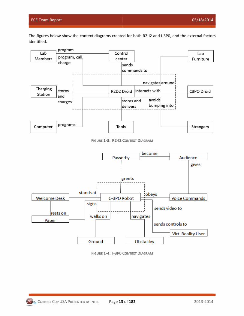
The figures below show the context diagrams created for both R2-I2 and I-3P0, and the external factors
identified.
FIGURE 1-3: R2-I2 CONTEXT DIAGRAM
FIGURE 1-4: I-3P0 CONTEXT DIAGRAM

ECE Team Report 05/18/2014
CORNELL CUP USA PRESENTED BY INTEL Page 14 of 182 2013-2014
1.3.2 Timeline The timeline is a widely used tool to manage projects, it allows the team to see what needs to be
accomplished and what everyone is working on. An excerpt of the Cornell Team’s timeline is shown below.
Start Date Completed Date
Team Member T
ime A
ctu
al
(hrs
) T
ime R
eq
(h
rs)
Eff
ort
(1-5
)
Dep
en
den
t O
n
ID
Su
b I
D#s
Milestone Task Deliverables
PD Project Definition
9/16/2013 9/16/2013 All 1 2 1 * 1 Define goals of each of the projects
All team members know what the final product is supposed to do
9/16/2013 9/16/2013 Team Leads
0.5 2 1 2 Determine Use Cases Context diagram. Use case Matrix
9/16/2013 9/16/2013 Team Leads
1 6 3 3 Determine Requirements Originating Requirements
9/16/2013 9/16/2013 Team Leads
0.5 2 1 4 Determine Subsystems List of main subsystems
9/16/2013 9/16/2013 All 2 8 4 5 List initial feasibility issues
List of potential feasibility issues and concern level in terms of at least uncertainty, time, and resource usage; Potential start of a FMEA matrix
9/16/2013 9/16/2013 All 3 2 1 6 Brainstorm solutions List of possible approaches, ranked by difficulty
9/16/2013 9/16/2013 Team Leads
2 4 2 7 Functional Flow Diagram Functional flow diagram
9/16/2013 9/16/2013 All 4 2 1 8 Determine equipment needed
List of equipment needed
9/16/2013 9/16/2013 All 5 2 1 9 Check for equipment availability
List of equipment not available in lab
TABLE 1-1: TIMELINE EXCERPT
Given the amount of work needed to develop not one, but two working robots within the span of two
semesters, having clear deliverables makes it easier to have tangible progress. Having well-defined
deliverables increases team morale because team members can see the team’s progress as the project
moves forward. Additionally, the timeline can help keep track of when important pieces of information
have to be relayed to other teams, for example the interface requirements for communication between
the robot software and the FPGA. Keeping track of start and end dates and actual time spent on each
activity informs future team leaders about what to expect regarding each of the tasks and will help them
plan accordingly.
2 FPGA Development Board Design Introduction
Following from the development work of the previous year’s ModBot, the Cornell team’s design approach
involves an embedded system. This means that we are using a computational system that monitors and
controls physical processes, such as monitoring the battery’s voltage, motor controls and feedback, and a
number of different sensors and sensing equipment, among other aspects of the robot.

ECE Team Report 05/18/2014
CORNELL CUP USA PRESENTED BY INTEL Page 15 of 182 2013-2014
In order to accomplish this, the Cornell team is utilizing a development board that includes a Field
Programmable Gate Array (FPGA). FPGAs are Integrated Circuits consisting of several logic blocks, which
can be configured for a particular functionality by the customer after the manufacturing process has been
completed. The several logic blocks that make up the FPGA can be wired together in hardware using
hardware description languages, such as Verilog or VHDL. In our designs, we have used Verilog.
By using the FPGA, we were able to develop embedded hardware that is capable of accomplishing much
of the low-level processing required to run the robot. This is beneficial for a couple of reasons. First off,
some computations can be performed quicker when handled directly by hardware specifically designed
to accomplish them versus an approach of software computation. It was our goal to use this to our
advantage to preprocess data prior to relaying it to the robot’s software. By doing this, we also free up
processor and memory resources at the software level. The end result was that we were able to utilize
the FPGA as an interface between the robot software and the robot peripherals.
Another benefit to using a FPGA is that it is easily reconfigurable, as it can be reprogrammed in seconds.
This allowed the Cornell team to rapidly prototype and test the hardware design throughout
development. The FPGA circuitry itself is developed as software code, where the inputs and outputs from
the circuitry are defined, as well as the internal computations. This was extremely useful as large changes
to the design could be implemented quickly in the code, and the FPGA could then be reprogrammed,
taking on a brand new functionality set.
2.1.1 Selected FPGA Development Board Due to the similar needs of the two robots (such as power regulation, motor control, and sensor
management) and the limited development time and resources, the decision was made to utilize the same
development board, the Terasic DE2i-150, for both robots. This particular board includes, among other
features, the Altera Cyclone IV 4CX150 FPGA, and the Intel Atom N2600, which includes an embedded
computer that we used to run the robots’ software.
Available to the Cyclone IV are 4 push buttons, 18 slide switches, 27 LED indicators, a serial connection, a
16x2 LCD module and a 40-pin expansion header. These features provided both human and peripheral
input and output and were at our disposal to use however we chose by accessing them with the FPGA.
FIGURE 2-1: DE2I-150 FPGA DEVELOPMENT BOARD

ECE Team Report 05/18/2014
CORNELL CUP USA PRESENTED BY INTEL Page 16 of 182 2013-2014
The FPGA itself connects to the Intel Atom portion of the DE2i-150 through a PCIe connection. Figure 2-2
below shows a block diagram of how the DE2i-150 is arranged.
FIGURE 2-2: BLOCK DIAGRAM OF THE DE2I-150
The Intel Atom portion of the DE2i-150 is used to run the robots’ code and communicate with the FPGA.
This portion acts as an embedded computer on the robot, running Windows 7. The interfaces between
the FPGA and the software code were developed in conjunction with the Computer Science Cornell Cup
team.
2.1.2 Additional DE2i-150 Documentation and Resources Additional information for the DE2i-150 development board can be found on Terasic’s website. Terasic is
the exclusive provider of Altera University Program FPGA development kits and provided Cornell’s team
with the Altera DE2i-150 development board.
Documentation and resources specific to the DE2i-150 can be found at the following URL: http://www.terasic.com.tw/cgi-bin/page/archive.pl?Language=English&CategoryNo=165&No=529&PartNo=5
Setting up the FPGA Board As previously mentioned, the Terasic DE2i-150 FPGA board, containing the Altera Cyclone IV GX FPGA,
was selected for use with both R2-I2 and I-3P0. This section provides an overview of how to connect and
configure the FPGA for development.
2.2.1 Install Required Development Software The Altera Complete Design Suite provides the necessary tools used for developing hardware and
software solutions for Altera FPGAs. The Quartus II software is the primary FPGA development tool used
to create reference designs, along with the Nios II Soft-Core Embedded Processor Integrated Development
Environment, which are both included in the package DVDs.

ECE Team Report 05/18/2014
CORNELL CUP USA PRESENTED BY INTEL Page 17 of 182 2013-2014
If you do not have access to the DVDs, the latest version of the software can be obtained from Altera’s
website: http://www.altera.com/download
The Web Edition of Quartus II supports developing and programming the Cyclone IV GX device on the
DE2i-150. If you choose to install the Subscription Edition, please note that a purchased license will be
required. For more information on the Subscription Edition, please go to the following link:
http://www.altera.com/products/software/quartus-ii/subscription-edition/qts-se-index.html
Once the software has been obtained, follow the steps in the following sections to install the Altera
Complete Design Suite.
Note: If all of the install files for Quartus II, the Cyclone IV FPGA support file, and ModelSim-Altera Edition
are in the same directory, running the Quartus II install will identify the files and allow for all three to be
installed within a single install session.
2.2.1.1 Quartus II Web Edition The following steps outline how to install the Quartus II Web Edition software. In order to complete the
Quartus II installation, the device support for the Cyclone IV FPGA must be installed. This can also be
obtained from either the DVD or the Altera website.
1. Download or retrieve from the DVD the Quartus II executable QuartusSetupWeb-X.X.X.X.exe. (The
latest version compatible with the DE2i-150 is recommended.)
2. Download or retrieve from the DVD the device support file for the Cyclone IV FPGA cyclone_web-
X.X.X.X.qdz and place it in the same directory as the executable from step 1
3. Run the executable QuartusSetupWeb-X.X.X.X.exe.
FIGURE 2-3: ALTERA QUARTUS II WEB EDITION INSTALLATION
4. Click Next.
5. Accept the agreement and click Next.
6. Select the desired install directory and click Next.

ECE Team Report 05/18/2014
CORNELL CUP USA PRESENTED BY INTEL Page 18 of 182 2013-2014
7. Ensure that the device support for the Cyclone IV is included in the list of components to install and
click Next.
FIGURE 2-4: CYCLONE IV DEVICE SUPPORT COMPONENT INSTALL
8. Click Next.
9. Once the install completes, click Finish.
2.2.1.2 ModelSim-Altera Edition The following steps outline how to install the ModelSim-Altera Edition software.
1. Download or retrieve from the DVD and run the executable, ModelSimSetup-X.X.X.X.exe. (The latest
version compatible with the DE2i-150 and Cyclone IV is recommended.)
FIGURE 2-5: MODELSIM-ALTERA EDITION INSTALLATION
2. Click Next.

ECE Team Report 05/18/2014
CORNELL CUP USA PRESENTED BY INTEL Page 19 of 182 2013-2014
3. Select ModelSim-Altera Starter Edition, unless you have a license for the full edition, and click Next.
4. Accept the agreement and click Next.
5. Select the desired install directory and click Next.
6. Click Next.
7. Once the install completes, click Finish.
2.2.1.3 Example Code In order to run the example code that is provided with the DE2i-150, it is recommended that it is copied
from the DVD (or downloaded zip file) to a local directory on the host computer. To do so, simply copy
the Demonstrations folder from the source (zip file or DVD) to the computer. These examples can be
loaded to the FPGA for testing purposes and to help understand how code runs on the FPGA.
2.2.2 Power On and Connect the FPGA Once the development software is installed, the FPGA can be powered on and connected. Follow these
steps to do so:
1. Connect 12V power supply to the DE2i-150 board’s power connector (J1) and plug it in. If the power
source is active and the power supply is working, the 12V LED (D33) will light up.
2. Press the POWER_ON/OFF button (PB1) to turn on the FPGA.
3. Once the FPGA is powered up, you should see the LEDs flashing, the 7-segment displays cycling
through the hexadecimal numbers, and the LCD outputting “Welcome to the DE2i-150”
4. Plug USB cable from the board’s USB connector (J9) into to your computer.
5. If the Altera USB-Blaster driver has not previously been installed, perform the following steps:
a) Navigate to Device Manager Other Devices USB-Blaster on the host computer.
b) Double-click on USB-Blaster.
c) In the Properties window, click on Update Driver.
d) Browse to the path where the driver is located and select it
(e.g. C:\<Quartus II install directory>\drivers\usb-blaster).
2.2.3 Programming the FPGA This is a quick guide to programming the FPGA board using the Quartus II programmer. This section tells
how to install a compiled .sof file, for the purposes of testing, any of the example projects can be
programmed to the FPGA.
For more detailed steps, please refer to Chapter 5 in the DE2i-150_Getting_Started_Guide.pdf found on
the board’s documentation page at the following URL
http://www.terasic.com.tw/cgi-bin/page/archive.pl?Language=English&CategoryNo=139&No=529&PartNo=5
1. Connect power supply and USB cable as described in the previous section.
2. Switch SW19 on the DE2i-150 to the RUN position.
3. Launch the Quartus II application.
4. Navigate to Tools Programmer.
5. In the Programmer window that appears, click Hardware Setup.
6. Ensure that USB-Blaster [USB-0] is selected in the Currently Selected Hardware menu and then close
the window.

ECE Team Report 05/18/2014
CORNELL CUP USA PRESENTED BY INTEL Page 20 of 182 2013-2014
7. Back in the Programmer window, click Add File and select the desired .sof file
a) For example, navigate to the Demonstrations folder that was downloaded from the CD, traverse
to \Demonstrations\FPGA\My_First_FPGA, and select my_first_fpga.sof
8. Check the Program/Configure box only for the desired .sof file
9. Click Start and the file will begin to download onto the board.
10. Once it has downloaded, your code will be running on the FPGA board.
a) The My_First_FPGA example should flash the four LEDs (LEDG0 to LEDG3) at different
frequencies. If you see this, congrats! You have loaded your first program onto the DE2i-150
board! :)
2.2.4 Installing Windows 7 In order to run the Intel Atom portion of the DE2i-150 development board, an operating system needs to
be installed. Terasic recommends Yocto Linux be installed, and if that is your preference, there is no reason
not to. It comes pre-loaded on the DE2i-150, so no operating system install is required if Linux is the
desired operating system. The Cornell Team installed Windows 7 in order to reuse code from the previous
years that was already coded in a Windows environment using Visual Studio. To limit the amount of
rework, and to accommodate the CS team, the decision was made to use Windows early on in the lifecycle
of the project.
Initially, the Cornell Team installed Windows 7 Embedded, but we were unable to get it to configure
correctly and establish the PCIe communications. A standard install of Windows 7 was tried after nothing
seemed to work to correct the problem in Windows 7 Embedded, and the problem was not present. From
that point on, Windows 7 was used.
The communication between the Intel Atom portion of the DE2i-150 board and the Cyclone IV FPGA uses
a PCIe connection. Terasic provided driver files for both Linux and Windows, both with extremely similar
function calls, so the impact to the ECE team was anticipated to be minimal. Unfortunately, the Windows
drivers and code were not well documented and caused a few issues establishing communications. These
issues are covered more in depth later in this document.
In order to install Windows 7 Embedded, perform the following steps:
1. Download Windows 7 Embedded from Microsoft, or from DreamSpark if you have an account.
http://www.microsoft.com/windowsembedded/en-us/windows-embedded-standard-7.aspx
a) The download should be done on a PC (not on the Intel Atom board)
2. Create a bootable USB using the download tool found at the following url:
http://www.microsoftstore.com/store/msusa/html/pbPage.Help_Win7_usbdvd_dwnTool
3. While the Intel Atom board is off, plug in the USB pen drive
a) Also connect a keyboard, mouse, and VGA monitor (into “VGA CPU” port, not the “VGA FPGA” or
“RS-232” port) so you can proceed with the installation.
4. Turn on the Intel Atom board and boot from the USB drive
a) After a loud beep, the Intel Atom will start the BIOS
5. Press the F10 key on the keyboard immediately to enter Boot Settings.
6. Select the USB drive as the bootable media in order to boot into the Windows Installation.
7. Follow the steps for Windows Installation:

ECE Team Report 05/18/2014
CORNELL CUP USA PRESENTED BY INTEL Page 21 of 182 2013-2014
a) Since Yocto is already installed on the Intel Atom Board, you may want to delete the existing
installation to install Windows.
b) When choosing where to install Windows, delete the partition with Yocto. Important: Note the
size of the partition, as you will be recreating it in the next step.
c) Create a new partition of the same size as the partition deleted in the last step.
d) Choose this partition for Windows Installation.
e) If prompted to choose between a Default Installation or a Basic installation, chose the Default
Installation.
8. Once Windows is finished installing, reboot the Intel Atom board.
a) The Intel Atom board should automatically start up Windows.
9. Install the provided drivers as mentioned in the Windows 7 installation Guide, which can be found at
the following url: http://www.intel.com/content/dam/www/public/us/en/documents/guides/installing-windows-7-os-de2i-150-board-guide.pdf
10. Download the Ethernet driver on a separate PC from Intel’s website:
http://downloadmirror.intel.com/18713/eng/PROWin32.exe
11. Transfer the driver to the Intel Atom board using a USB drive and run the application.
12. Download the WiFi driver from Intel’s website:
http://downloadmirror.intel.com/22547/eng/Wireless_15.6.1_Ds32.exe
13. Transfer the driver to the Intel Atom board using a USB drive and run the application.
14. Copy the PCIe-FPGA driver from the System CD to the Intel Atom board using a USB drive. The driver
files are located in the following directory: /Demonstrations/PCIe_SW_KIT/Windows/.
15. Once transferred to the Intel Atom board, navigate to the PCIe_DriverInstall folder and run the
PCIe_DriverInstall.exe application. Note, the files can also be found online at the following URL:
http://www.terasic.com.tw/cgi-bin/page/archive.pl?Language=English&CategoryNo=11&No=529
FIGURE 2-6: PCIE DRIVER INSTALL FILE
a) Click Install and then OK.

ECE Team Report 05/18/2014
CORNELL CUP USA PRESENTED BY INTEL Page 22 of 182 2013-2014
FIGURE 2-7: PCIE DRIVER INSTALLATION
16. At this point, the installation of Windows is complete and the necessary drivers should be configured.
2.2.5 Starting New Project 1. Launch the Quartus II software
2. Click Create a New Project.
3. At the splash screen that appears, click Next.
4. Enter the project name and working directory and click Next.
5. Add desired files, if any, and click Next.
6. You should now be at the Family and Device Settings screen. Make sure to choose Cyclone IV GX for
Device Family and EP4CGX150DF31C7 for the Device Name.
7. Click Finish.
8. Start coding!
9. Refer to the Setting up Pins section of this document after writing code, but before compiling.
2.2.6 Editing Code 1. Open the desired .qpf project file.
a) Navigate to the Demonstrations folder that was downloaded from the CD or the website.
b) Navigate to \Demonstrations\FPGA\My_First_FPGA.
c) Double-click on my_first_fpga.qpf to launch the project in Quartus II.
i) Alternatively, launch Quartus II and click Open Existing Project
ii) Or, launch Quartus II and open the .qpf file from within Quartus by navigating to File Open
Project.
2. Edit the desired files and save the project.
3. If the pins have not been set up yet, please refer to the Setting up Pins section of this document
4. Compile the code by selecting Processing Start Compilation.
5. Follow steps in the Programming the FPGA section of this document.
2.2.7 Example Program A simple program was implemented to get an understanding of the FPGA Expansion header, the Quartus
II environment and the DE2i-150 board. The example program was aimed at receiving an input from a
switch, via PIN G_16 and switching on/switching off the LED, connected to PIN F_17. PIN G_16 was
configured as an input, while F_17 was configured as an output. The simple circuitry used for this program
is illustrated below.

ECE Team Report 05/18/2014
CORNELL CUP USA PRESENTED BY INTEL Page 23 of 182 2013-2014
FIGURE 2-8: CIRCUIT FOR LED-SWITCH SAMPLE PROGRAM
When the switch was pressed, the LED would glow. This program helped us understand the usage of GPIO
ports for external input and output circuitry.
Pulse Width Modulation Pulse Width Modulation (PWM) is a simple digital to analog conversion technique that does not require
an ADC. PWM signals are used as inputs from the sensors to the FPGA. They are also used as outputs from
the FPGA to drive the servos. Therefore, it was decided to implement PWM Input and Output modules in
the FPGA. The 35 GPIO (General Purpose Input/Output) Expansion header of the DE2i-150 is used for the
PWM modules. Since, the project uses a large number of sensors, a decision was made to utilize the 35
GPIO ports of the DE2i-150, to overcome the restriction due to limited I/O Port supported by the Intel
Atom processor. Though FPGA is used, most of the design implementation will be carried out on the Intel
Atom processor. This requires effective communication between Intel Atom and FPGA. This is achieved
with the help of the PCIe protocol. Refer the PCI Communication Setup section later in this document for
a more detailed explanation.
2.3.1 PWM Input A PWM capture module has been implemented for the FPGA. The Hardware Description Language (HDL)
used for this implementation is Verilog. The module is capable of receiving a PWM signal as an input and
computing the duty cycle as an output parameter.
2.3.1.1 Design
The design consists of a the master module, which receives the input data, in the form of a PWM signal,
from an external source and computes the Duty Cycle, or the time duration of the high part of the signal
in terms as percentage of the total period of the signal. A simple block diagram of the module is provided
in the following figure:

ECE Team Report 05/18/2014
CORNELL CUP USA PRESENTED BY INTEL Page 24 of 182 2013-2014
FIGURE 2-9: BLOCK DIAGRAM FOR PWM INPUT
As evidenced in the block diagram, the master module Sensor consists of two input ports and two output
ports. The Input port, clk is connected to the output port of a Phase-Locked Loop (PLL) Megafunction
module, the input to which is one of the 50MHz crystal oscillators used in the DE2i-150 boards. The signal
properties of the PLL module (frequency, pre-scaling value, etc.) can be selected by clicking on the
Megafunction plugin. For more information refer to Altera’s documentation, My First FPGA Design
Tutorial, specifically the Add a PLL Megafuntion section. This file can be found on Altera’s site at the
following URL: http://www.altera.com/literature/tt/tt_my_first_fpga.pdf
The properties for the PLL module used in our design are stated below:
inclk0 Frequency = 50MHz
Clock = c0
Operation mode = Normal
Duty Cycle = 50%
Prescaler = 1
The Output of the PLL module, c0 is connected to the input port clk of the module Sensor. The other input
port of the module Sensor, Signal, is mapped to PIN G_16 (GPIO[0]) of the expansion header. The PWM
signal from an external source is fed into the module via this pin.
Upon receiving the input signal at PIN G_16, the signal is delayed for two clock cycles before analysis in
order to weed out phase difference between the internal clock and the clock signal of the source. Figure
2-10 below describes the clock synchronization concept adapted for the module.
ECE Team Report 05/18/2014
CORNELL CUP USA PRESENTED BY INTEL Page 25 of 182 2013-2014
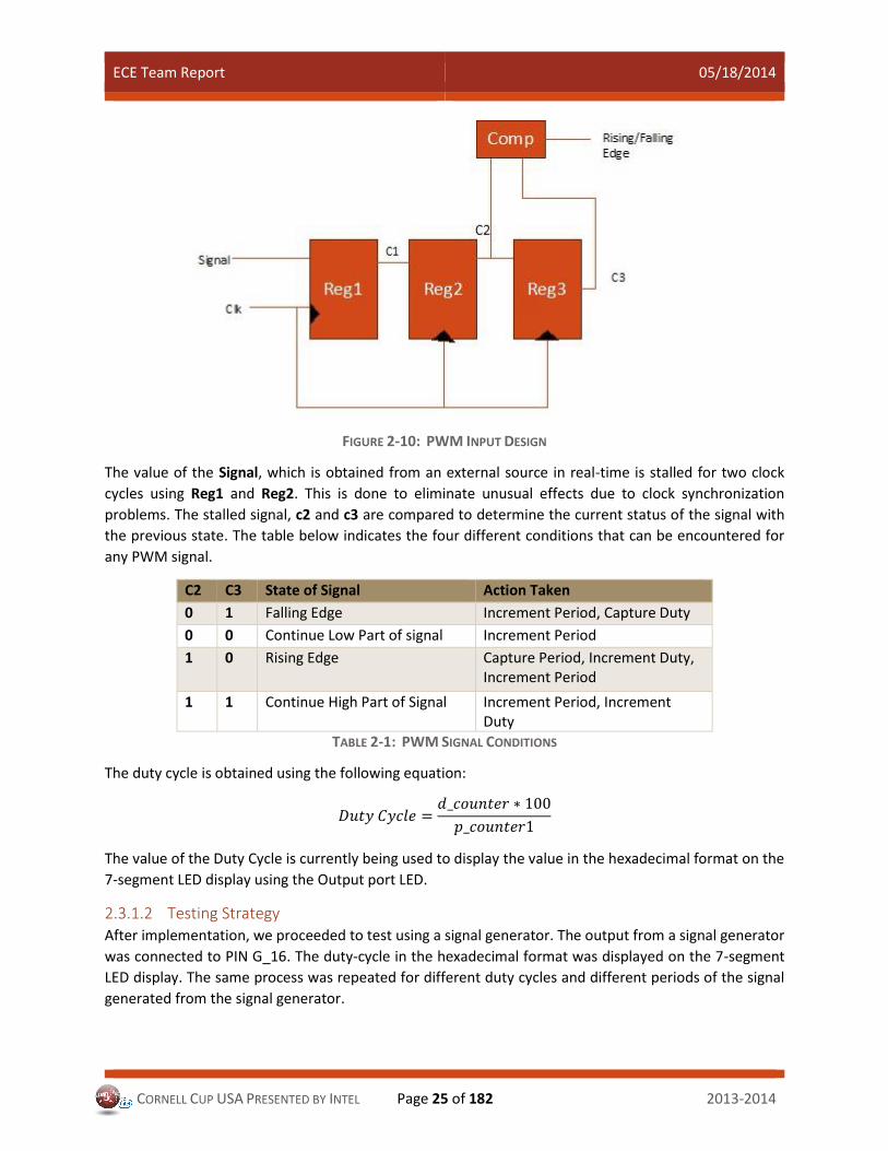
FIGURE 2-10: PWM INPUT DESIGN
The value of the Signal, which is obtained from an external source in real-time is stalled for two clock
cycles using Reg1 and Reg2. This is done to eliminate unusual effects due to clock synchronization
problems. The stalled signal, c2 and c3 are compared to determine the current status of the signal with
the previous state. The table below indicates the four different conditions that can be encountered for
any PWM signal.
C2 C3 State of Signal Action Taken
0 1 Falling Edge Increment Period, Capture Duty
0 0 Continue Low Part of signal Increment Period
1 0 Rising Edge Capture Period, Increment Duty, Increment Period
1 1 Continue High Part of Signal Increment Period, Increment Duty
TABLE 2-1: PWM SIGNAL CONDITIONS
The duty cycle is obtained using the following equation:
𝐷𝑢𝑡𝑦 𝐶𝑦𝑐𝑙𝑒 =𝑑_𝑐𝑜𝑢𝑛𝑡𝑒𝑟 ∗ 100
𝑝_𝑐𝑜𝑢𝑛𝑡𝑒𝑟1
The value of the Duty Cycle is currently being used to display the value in the hexadecimal format on the
7-segment LED display using the Output port LED.
2.3.1.2 Testing Strategy After implementation, we proceeded to test using a signal generator. The output from a signal generator
was connected to PIN G_16. The duty-cycle in the hexadecimal format was displayed on the 7-segment
LED display. The same process was repeated for different duty cycles and different periods of the signal
generated from the signal generator.

ECE Team Report 05/18/2014
CORNELL CUP USA PRESENTED BY INTEL Page 26 of 182 2013-2014
Further testing is necessary once the PCIe is complete and working to ensure that the implementation is
correct. An analysis of the data dump can be obtained from the hyperterminal once PCIe is implemented.
2.3.1.3 Issues Faced A major issued that was faced was the difference in phase of the clocks of the PWM Input module and the
source signal. As previously mentioned, this was overcome by delaying the processing by two clock cycles.
The other major issue faced was that the design was erratic for 𝑝𝑒𝑟𝑖𝑜𝑑 < 200 𝐾ℎ𝑧. This was overcome
by increasing the range of d_counter0 and p_counter1 registers from [15:0] to [31:0]. In the future, this
may be further increased if necessary.
2.3.2 PWM Output PWM stands for Pulse Width Modulation. This means that we can generate a pulse of specified width (i.e.
duration). PWM Output, having a periodic rectangular signal, can be used to control a device by changing
the duty cycle (the percentage of time that the output pin is high). The PWM input can be of any width,
such as 8-bits or 16-bits, but the PWM output is just one-bit wide.
2.3.2.1 Design The design consists of a Verilog module, which receives the input data, in the form of 8 switches to control
the PWM output. By changing input from switches, we can see the PWM output changing on the
oscilloscope. A simple block diagram of the module is provided in the figure below.
FIGURE 2-11: BLOCK DIAGRAM FOR PWM OUTPUT
The main module PWM_verilog consists of two input ports and one output port. The Input port, clk is
connected to the output port of a Phase-Locked Loop Mega function module, the input to which is one of
the 50MHz crystal oscillators used in the DE2i-150 boards. The signal properties of the PLL module (namely
frequency, pre-scaling value, etc.) can be selected by clicking on the Megafunction plugin. For more
information refer to http://www.altera.com/literature/tt/tt_my_first_fpga.pdf, section Add a PLL
Megafuntion. The properties for the PLL module used in our design are the following:

ECE Team Report 05/18/2014
CORNELL CUP USA PRESENTED BY INTEL Page 27 of 182 2013-2014
inclk0 Frequency = 50MHz
Clock = c0
Operation mode = Normal
Duty Cycle = 50%
Prescaler = 1
The Output of the PLL module, c0 is connected to the input port clk of the module PWM_verilog. The
other input port of the module PWM_verilog, switches, is mapped to 8 switches (pin details are shown
above in Figure 2-11).
Initially, we have to specify the frequency at the signal will be refreshed, which in this case is 𝑡 = 1 𝑚𝑠𝑒𝑐.
Next, the wave Period, P, can be calculated. The period is the number of clock steps after which the signal
will refresh. This is done using the following equation:
𝑃𝑒𝑟𝑖𝑜𝑑 = 𝑡 ∗ 𝐹𝑃𝐺𝐴 𝑐𝑙𝑜𝑐𝑘 𝑠𝑝𝑒𝑒𝑑 = 0.001 ∗ 50000000 = 50000
This means that the signal refreshes every 50000 clock steps. This value determines the counter for our
module which is used as our duty cycle. Since the maximum steps a clock can take are 50000, the counter
only needs to go up to 5000. The number of bits needed for the counter can be calculated using 𝑙𝑜𝑔2(𝑃).
𝑙𝑜𝑔2(𝑃) = 𝑙𝑜𝑔2(50000) = 15.6
Rounding up to the nearest integer (i.e. 16 bits), works nicely for computer code. 8 switches are available,
which means that we can count from 0 to 255, since the step count is 28 = 256.
The next step is to calculate step delay. This is done with the following equation:
𝑆𝑡𝑒𝑝 𝐷𝑒𝑙𝑎𝑦 =𝑃𝑒𝑟𝑖𝑜𝑑
𝑆𝑡𝑒𝑝 𝑐𝑜𝑢𝑛𝑡
=50000
256= 195
For example, let’s say the output voltage is 5V. If the signal is halved, which can be calculated as 27 =
128, then only the lower are 7 bits on, resulting in a signal of 2.5V.
2.3.2.2 Testing Strategy After implementation, testing was done using an oscilloscope. The input from the switches was changed
for values ranging from 0 to 256. We were able to see the different outputs corresponding to individual
inputs because the PWM stays high based on the input switches. The tested input switches and
corresponding number of steps for which PWM stays high is shown in Table 2-2: PWM Test Expected
Results.
Switches Count of switches PWM stays HIGH (steps)
11111111 255 49725
10000000 128 24960
01000000 64 12480

ECE Team Report 05/18/2014
CORNELL CUP USA PRESENTED BY INTEL Page 28 of 182 2013-2014
00100000 32 6240
00010000 16 3120
00000010 2 390
00000001 1 195
00000000 0 0
TABLE 2-2: PWM TEST EXPECTED RESULTS
Further testing is necessary once the PCIe is complete and working to ensure that the implementation is
correct. An analysis of the data dump can be obtained from the hyperterminal once PCIe is implemented.
2.3.3 Creating the Verilog Program Follow the below steps to make the same program in Verilog on Quartus II.
1. Launch the Quartus II software.
2. Select File New Project Wizard.
3. When the Introduction page opens, click Next.
4. Enter the following information about your project:
a) What is the working directory for this project? Enter a directory in which you will store your
Quartus II project files for this design.
i) For example, E:\My_design\PWM.
ii) File names, project names, and directories in the Quartus II software cannot contain spaces.
b) What is the name of this project? Type my_first_fpga.
c) What is the name of the top-level design entity for this project? Type my_first_fpga.
Matrix Multiplication using FPGA Matrix Multiplication is a basic operation that can be used in many applications. FPGA are able to
accelerate the matrix multiplication computation using parallelism. This leads to high performance
improvements in any intensive data processing problems. Implementing matrix multiplication
demonstrates the performance of the FPGA in solving computationally intensive problems.
2.4.1 Design The design consists of a Verilog module, which receives the input data from 8 switches and displays the
results using LED0. A simple block diagram of the module is shown in Figure 2-12: Block Diagram for
Matrix Multiplication Output.

ECE Team Report 05/18/2014
CORNELL CUP USA PRESENTED BY INTEL Page 29 of 182 2013-2014
FIGURE 2-12: BLOCK DIAGRAM FOR MATRIX MULTIPLICATION OUTPUT
The main module Matrix_verilog consists of two input ports and one output port. The Input port, clk is
connected to the output port of a Phase-Locked Loop Megafunction module, the input to which is one of
the 50MHz crystal oscillators used in the DE2i-150 boards. The signal properties of the PLL module, namely
frequency, pre-scaling value etc. can be selected by clicking on the Mega function plugin. For more
information refer to http://www.altera.com/literature/tt/tt_my_first_fpga.pdf, section Add a PLL
Megafuntion. The properties for the PLL module used in our design are stated below:
inclk0 Frequency = 50MHz
Clock = c0
Operation mode = Normal
Duty Cycle = 50%
Prescaler = 1
The output of the PLL module, c0 is connected to the input port clk of the module Matrix_verilog. The
other input port of the module Matrix_verilog, switches, is mapped to 8 switches (pin details are shown
above in Figure 2-12).
Input is taken from switches 1-4 in Matrix 1 and from switches 5-8 in Matrix 2. Then, each time the inputs
are changed, we are resetting the result using reset function of FPGA board and calculating the
multiplication again. The result is displayed in LED0 using its seven segments.
2.4.2 Testing Strategy After implementation, the module was tested by changing various input combinations using switches.
The input from the switches can be either 0 or 1. Using this approach, the maximum value reached by the

ECE Team Report 05/18/2014
CORNELL CUP USA PRESENTED BY INTEL Page 30 of 182 2013-2014
matrix multiplication result is 4. The tested input switches and the respective output is shown in table
Table 2-3: Matrix Multiplication Expected Results.
Result LED Seven Segments Input 1 Input 2
0 1000000 0000 0001
1 1111001 0001 1111
2 0100100 0011 0111
3 0110000 1110 1110
4 0011001 1111 1111
TABLE 2-3: MATRIX MULTIPLICATION EXPECTED RESULTS
Further work on this function is required to accommodate all the data requests from sensors and servos.
Enhancement of this matrix multiplication function can be used for Image processing applications on FPGA
using Sobel filters.
Intel Atom Communication In order to communicate between the FPGA to the Intel Atom, the PCIe communications bridge must be
utilized. The following subsections detail how to set up the initial communication as well as how to code
using the PCIe libraries.
2.5.1 PCI Communication Setup 2.5.1.1 Requirements 1. PCI Drivers (located on the CD or downloaded from the Terasic website)
2. Visual Studio 2012 (must be 2012 version in order to run code provided by Intel)
3. PCI Header and C files
4. Intel Code for Intel Atom (app.c)
5. PCIE_Fundamental code for FPGA (from the CD)
2.5.1.2 Steps 1. Ensure Windows 7 (the full version, not Embedded) is installed on the Intel Atom.
2. Power on the DE2i-150 and boot Windows.
3. On a separate computer, load the /FPGA/de2i_150_qsys_pcie.sof file onto the FPGA. This can be
done two ways:
a) Go to PCIE_Fundamental/demo_batch, and run the “sof_download” batch file. Make sure that
the FPGA’s switch19 is in the RUN position.
b) Alternatively, one can follow the steps in 2.2.3 (Programming the FPGA) to use Quartus to load
the .sof onto the FPGA.
4. Once the .sof is loaded, navigate to the following directory on the Intel Atom board:
De2i-150_PCIe_Win/PCIE_SW_KIT/Windows/PCIe_DriverInstall
5. On the Intel Atom board, right-click on the PCIe_DriverInstall.exe executable and Run as
Administrator. Note that the .sof might need to be loaded on the board for the driver install to work.
6. Click Install.

ECE Team Report 05/18/2014
CORNELL CUP USA PRESENTED BY INTEL Page 31 of 182 2013-2014
FIGURE 2-13: PCIE DRIVER INSTALLER
7. Once done, navigate to Control Panel Device Manager
8. Expand Jungo.
9. Ensure that under Jungo, both the TERASIC PCIe FPGA Board and WinDriver devices show up.
FIGURE 2-14: DEVICE MANAGER
a) The TERASIC PCIe FPGA Board entry may have a yellow triangle in the icon; this is OK. If it does
not appear, follow these steps:
i) In device manager, Select Action Scan for hardware changes. If it still doesn’t show up, try
step ii.
ii) Rerun the driver installer again (multiple tries may be needed). If it still doesn’t work, restart
the Intel Atom board (shut down through Start menu) and try again.
10. Restart Windows through the Start menu (Do not hard reset the board!)
11. Navigate to the following directory and run the executable app.exe.
11-23-13/De2i-150_PCIe_Win/windows_app_vc2012/Release
12. The app.exe has four functions:
a) Zero controls the LEDs 0-3. For example, typing a 3 for the “mask” will light up LED’s 0 and 1.
b) One reads the status of the FPGA’s button inputs. For example, if button 1 is pressed down.
2.5.2 Coding the PCIe Communications The following procedures detail how to use the PCIe communications SDK files in a C/C++ project using
Visual Studio. The initial drivers received from Terasic did not work as expected, but through
communications with the company directly, we were able to obtain updated drivers and sample
applications. It is recommended that you obtain these either directly from Terasic (if they haven’t included
them in a subsequent release) or from the Cornell team.

ECE Team Report 05/18/2014
CORNELL CUP USA PRESENTED BY INTEL Page 32 of 182 2013-2014
1. Launch Visual Studio.
2. Create a new C/C++ project.
3. Ensure that the De2i-150_PCIe_Win directory containing the updated Terasic drivers and sample
projects are copied to your computer.
4. Copy the following files into your Visual Studio project directory:
• TERASIC_PCIE.h
• TERASIC_PCIE_QSYS.dll (Note: Use TERASIC_PCIE_QSYSx64.dll for 64 bit systems)
o This file will be required by the executable generated by compiling your project.
5. Include TERASIC_PCIE.h in the 32-bits C/C++ project.
6. Copy the TERASIC_PCIE_QSYS.dll library into the Build directory (if it exists, if not, copy it there after
the first time the program is compiled).
Prior to coding your own interfaces, it is recommended that you use the demo applications provided by
Terasic in order to first test the PCIe interface, as these are known to work properly.
2.5.2.1 PCIe Application Coding The application shows how to call the TERASIC_PCIE.DLL (TERAISC_PCIEx64.DLL under 64-bits Windows)
exported API. To enumerate all PCIe cards in system call, the software design defines some constant based
on FPGA design shown below:
#define PCIE_VID 0x1172 #define PCIE_DID 0xE001
#define DEMO_PCIE_USER_BAR PCIE_BAR1
#define DEMO_PCIE_IO_ADDR 0x04
#define DEMO_PCIE_FIFO_ID 0x00
The vendor ID is defined as 0x1172 and the device ID is defined as 0xE001. The BUTTON/LED register
address is 0x04 based on PCIE_BAR1.
A C++ class PCIE is designed to encapsulate the DLL dynamic loading for TERASIC_PCIE.DLL (loading
TERAISC_PCIEx64.DLL under 64-bits Windows). A PCIE instance is created with the name m_hPCIE. To
enumerate all PCIe cards in system, call the function
m_hPCIE.ScanCard(wVendorID, wDeviceID, &dwDeviceNum, mszPcieInfo);
where wVendorID and wDeviceID are zeros. The return value dwDeviceNum represents the number of
PCIe cards found in the system. The m_szPcieInfo array contains the detail information for each PCIe card.
To connect the selected PCIe card, the following functions are called:
int nSel = ComboBoxBoard->ItemIndex;
WORD VID = m_szPcieInfo9nSel].VendorID;
WORD DID = m_szPcieInfo(nSel].DeviceID; bSuccess = m_hPCIE.Open(VID,DID,0); //0: first matched board
where nSel is selected index in the ‘Selected FPGA Board’ pull-down menu. Based on the return
m_szPcieInfo, we can find the associated PID and DID which can be used to specify the target PCIe card.

ECE Team Report 05/18/2014
CORNELL CUP USA PRESENTED BY INTEL Page 33 of 182 2013-2014
To read the BUTTON status, the following function is called:
m_hPCIE.Read32(DEMO_PCIE_USER_BAR, DEMO_PCIE_IO_ADDR, &dwData);
To set LED status, the following function is called:
m_hPCIE.Write32(DEMO_PCIE_USER_BAR, DEMO_PCIE_IO_ADDR, &dwData);
To write and read memory-mapped memory, call the functions:
// write bSuccess = m_hPCIE.DmaWrite(LocalAddr, pWrite, nTestSize);
if (bSuccess) {
// read
bSuccess = m_hPCIE.DmaRead(LocalAddr, pWrite, nTestSize); }
To write and read FIFO memory, call the following functions:
bSuccess = m_hPCIE.DmaFifoWrite(FifoID, pWrite, nTestSize); if (bSuccess) {
// read
bSuccess = m_hPCIE.DmaFifoRead(FifoID, pWrite, nTestSize);
}
2.5.2.2 TERASIC_PCIE.h The following is a quick overview of the function calls included in TERASIC_PCIE.h
//===========================================================================
// function prototype used for "static load DLL"
#if 0
BOOL PCIE_API PCIE_ScanCard(WORD wVendorID, WORD wDeviceID, DWORD
*pdwDeviceNum, PCIE_CONFIG szConfigList[]); // PciVID/PciPID=0/0--> scan all
pci card
PCIE_HANDLE PCIE_API PCIE_Open(WORD wVendorID, WORD wDeviceID, WORD
wCardNum);
void PCIE_API PCIE_Close(PCIE_HANDLE hFPGA);
BOOL PCIE_API PCIE_Read32 (PCIE_HANDLE hFPGA, PCIE_BAR PciBar, PCIE_ADDRESS
PciAddress, DWORD *pdwData);
BOOL PCIE_API PCIE_Write32 (PCIE_HANDLE hFPGA, PCIE_BAR PciBar, PCIE_ADDRESS
PciAddress, DWORD dwData);
BOOL PCIE_API PCIE_DmaRead (PCIE_HANDLE hFPGA, PCIE_LOCAL_ADDRESS
LocalAddress, void *pBuffer, DWORD dwBufSize);

ECE Team Report 05/18/2014
CORNELL CUP USA PRESENTED BY INTEL Page 34 of 182 2013-2014
BOOL PCIE_API PCIE_DmaWrite (PCIE_HANDLE hFPGA, PCIE_LOCAL_ADDRESS LocalAddress, void *pData, DWORD dwDataSize);
BOOL PCIE_API PCIE_DmaFifoRead (PCIE_HANDLE hFPGA, PCIE_LOCAL_FIFO_ID LocalFifoId, void *pBuffer, DWORD dwBufSize);
BOOL PCIE_API PCIE_DmaFifoWrite (PCIE_HANDLE hFPGA, PCIE_LOCAL_FIFO_ID
LocalFifoId, void *pData, DWORD dwDataSize);
// interrupt
BOOL PCIE_API PCIE_IntIsEnabled (PCIE_HANDLE hFPGA);
BOOL PCIE_API PCIE_IntEnable (PCIE_HANDLE hFPGA, TERASIC_INT_HANDLER
funcIntHandler);
void PCIE_API PCIE_IntDisable (PCIE_HANDLE hFPGA);
#endif
//===========================================================================
// function prototype used for "dynamic load DLL"
typedef BOOL (PCIE_API *LPPCIE_ScanCard)(WORD wVendorID, WORD wDeviceID, DWORD *pdwDeviceNum, PCIE_CONFIG szConfigList[]);
typedef PCIE_HANDLE (PCIE_API *LPPCIE_Open)(WORD wVendorID, WORD wDeviceID,
WORD wCardNum);
typedef void (PCIE_API *LPPCIE_Close)(PCIE_HANDLE hFPGA);
typedef BOOL (PCIE_API *LPPCIE_Read32)(PCIE_HANDLE hFPGA, PCIE_BAR PciBar, PCIE_ADDRESS PciAddress, DWORD *pdwData);
typedef BOOL (PCIE_API *LPPCIE_Write32)(PCIE_HANDLE hFPGA, PCIE_BAR PciBar,
PCIE_ADDRESS PciAddress, DWORD dwData);
typedef BOOL (PCIE_API *LPPCIE_DmaRead) (PCIE_HANDLE hFPGA,
PCIE_LOCAL_ADDRESS LocalAddress, void *pBuffer, DWORD dwBufSize);
typedef BOOL (PCIE_API *LPPCIE_DmaWrite) (PCIE_HANDLE hFPGA,
PCIE_LOCAL_ADDRESS LocalAddress, void *pData, DWORD dwDataSize);
typedef BOOL (PCIE_API *LPPCIE_DmaFifoRead) (PCIE_HANDLE hFPGA,
PCIE_LOCAL_FIFO_ID LocalFifoId, void *pBuffer, DWORD dwBufSize);
typedef BOOL (PCIE_API *LPPCIE_DmaFifoWrite) (PCIE_HANDLE hFPGA,
PCIE_LOCAL_FIFO_ID LocalFifoId, void *pData, DWORD dwDataSize);
// interrupt
typedef BOOL (PCIE_API *LPPCIE_IntIsEnabled) (PCIE_HANDLE hFPGA);

ECE Team Report 05/18/2014
CORNELL CUP USA PRESENTED BY INTEL Page 35 of 182 2013-2014
typedef BOOL (PCIE_API *LPPCIE_IntEnable) (PCIE_HANDLE hFPGA, TERASIC_INT_HANDLER funcIntHandler);
typedef void (PCIE_API *LPPCIE_IntDisable) (PCIE_HANDLE hFPGA);
Store Programs on FPGA using Active Serial Mode Quartus II The general procedure to run Verilog programs on FPGA does not store the program on the device for
later use. We need to recompile the program each time after turning the power ON. But for Cornell Cup
project, we wanted to enable the device to store the programs and reconfigure automatically each time
the board is turned ON.
Altera’s DE-series board allows the configuration to be done in two different ways, known as JTAG and AS
modes. The configuration data is transferred from the host computer (which runs the Quartus II software)
to the board by means of a cable that connects a USB port on the host computer to the leftmost USB
connector on the board. In the JTAG mode, the configuration data is loaded directly into the FPGA device.
The acronym JTAG stands for Joint Test Action Group. If the FPGA is configured in this manner, it will retain
its configuration as long as the power remains turned on. The configuration information is lost when the
power is turned off. The second possibility is to use the Active Serial (AS) mode. In this case, a
configuration device that includes some flash memory is used to store the configuration data. Quartus II
software places the configuration data into the configuration device on the DE-series board. Then, this
data is loaded into the FPGA upon power-up or reconfiguration.
Perform the following steps to make the FPGA Device work in Active Serial Mode:
1. Connect power supply and USB cable to the Terasic DE2i-150 board.
2. Switch SW19 on the DE2i-150 to the RUN position.
3. Launch the Quartus II application. 4. Navigate to Tools Programmer.
5. In the Programmer window that appears, click Hardware Setup.
6. Ensure that USB-Blaster [USB-0] is selected in the Currently Selected Hardware menu and then close
the window.
7. Back in the Programmer window, click Add File and select the desired .sof file
a) For example, navigate to the Demonstrations folder that was downloaded from the CD, traverse
to \Demonstrations\FPGA\My_First_FPGA, and select my_first_fpga.sof
8. Click Assignments Device as shown in Figure 2-15.
FIGURE 2-15: SELECT DEVICE FROM QUARTUS II
9. Then you will see the Device window as in Figure 2-16.
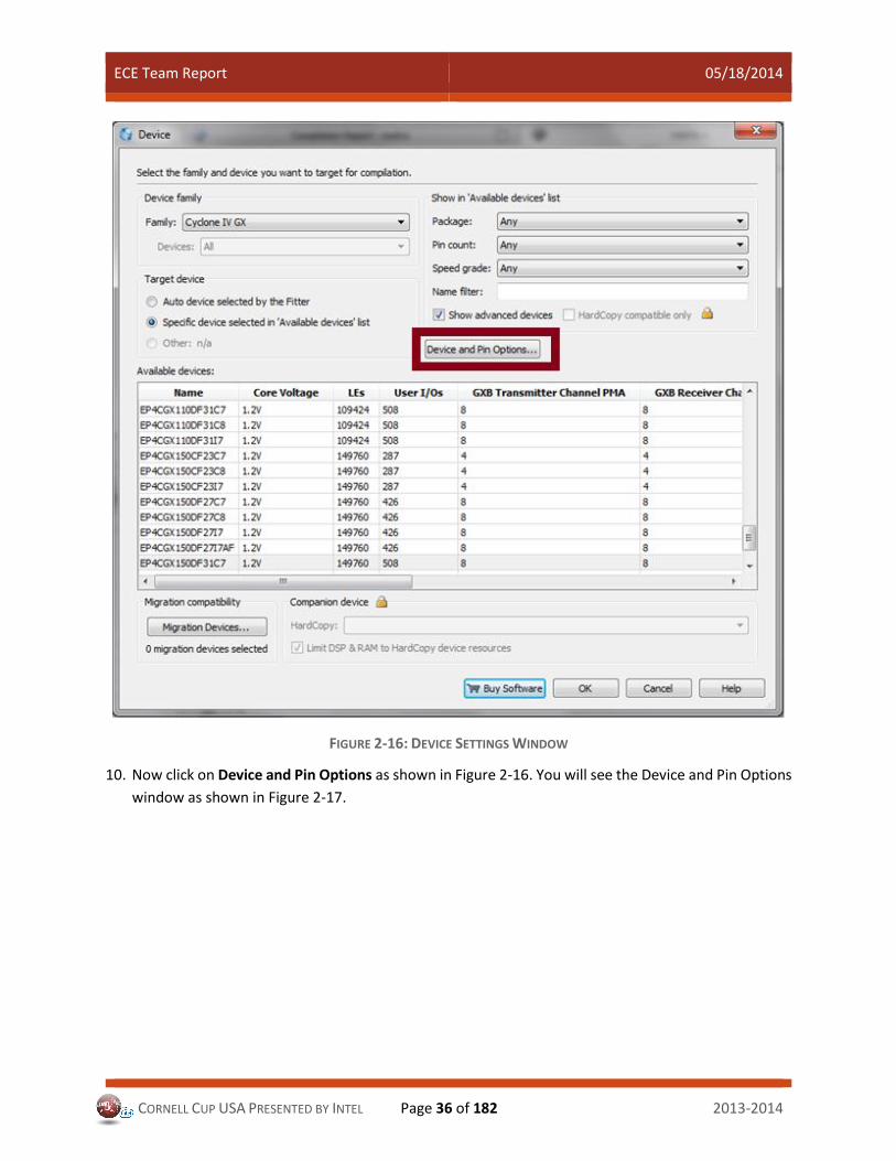
ECE Team Report 05/18/2014
CORNELL CUP USA PRESENTED BY INTEL Page 36 of 182 2013-2014
FIGURE 2-16: DEVICE SETTINGS WINDOW
10. Now click on Device and Pin Options as shown in Figure 2-16. You will see the Device and Pin Options
window as shown in Figure 2-17.

ECE Team Report 05/18/2014
CORNELL CUP USA PRESENTED BY INTEL Page 37 of 182 2013-2014
FIGURE 2-17: DEVICE AND PIN OPTIONS WINDOW
11. Click on the Configuration option from the left hand side as shown in Figure 2-17. Choose
Configuration Scheme as “Active Serial (can use Configuration Device)”.
12. Check “Use Configuration Device” and select the configuration for your respective board. For Terasic
DE2i-150 board, it is EPCS-64 (Figure 2-18).

ECE Team Report 05/18/2014
CORNELL CUP USA PRESENTED BY INTEL Page 38 of 182 2013-2014
FIGURE 2-18: SPECIFYING THE CONFIGURATION DEVICE
13. Click OK on Device and Pin Options Window and Device Window. This will get you back to the main
Quartus Window.
FOLLOW STEP 14 ONLY IF YOU DO NOT SEE THE ABOVE DEVICE SETTINGS. OTHERWISE THERE IS NO NEED
TO RECOMPILE.
14. Recompile the program by clicking Processing Start Compilation as shown in Figure 2-19.
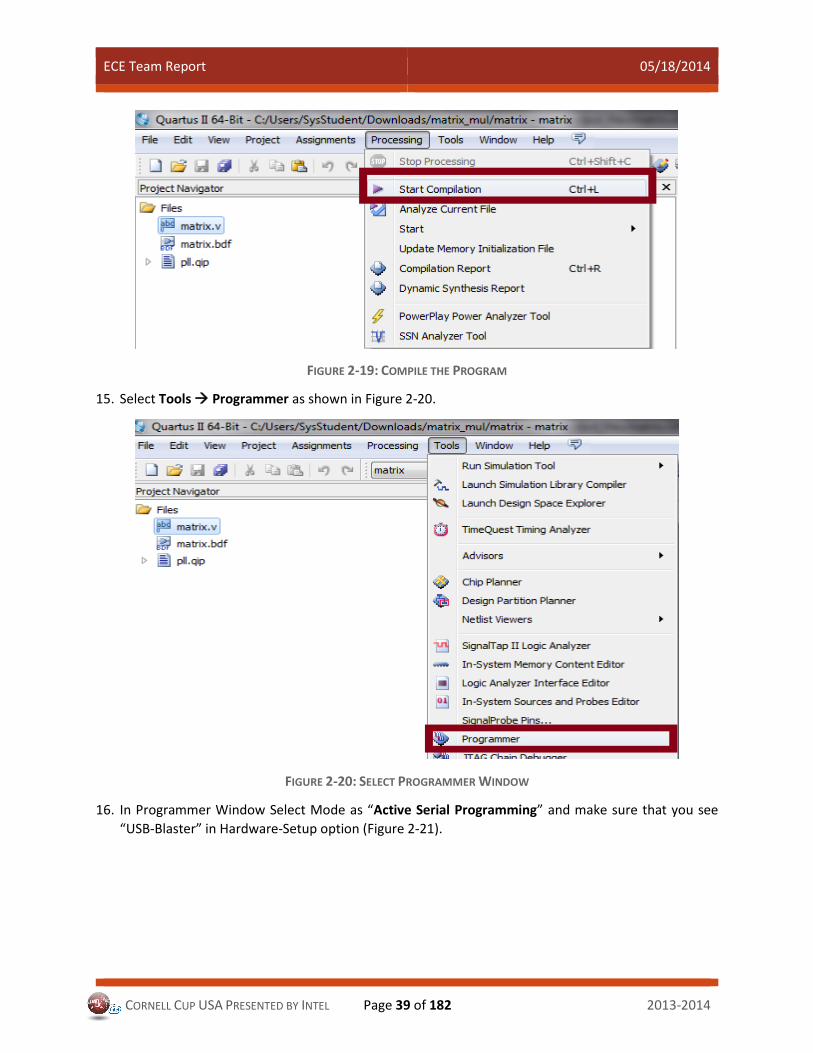
ECE Team Report 05/18/2014
CORNELL CUP USA PRESENTED BY INTEL Page 39 of 182 2013-2014
FIGURE 2-19: COMPILE THE PROGRAM
15. Select Tools Programmer as shown in Figure 2-20.
FIGURE 2-20: SELECT PROGRAMMER WINDOW
16. In Programmer Window Select Mode as “Active Serial Programming” and make sure that you see
“USB-Blaster” in Hardware-Setup option (Figure 2-21).

ECE Team Report 05/18/2014
CORNELL CUP USA PRESENTED BY INTEL Page 40 of 182 2013-2014
FIGURE 2-21: PROGRAMMER WINDOW
17. Flip the RUN/PROG switch on the DE-series board to the PROG position. Click Start and the file will
begin to download onto the board.
18. Once it has downloaded, your code will be running on the FPGA board.
19. When you are testing the design make sure the RUN/PROG switch on the DE-series board is at the
PROG position.
20. On the board, you should be able to see the PCI Driver in Device Manager under Jungo.
FIGURE 2-22: DEVICE MANAGER WINDOW
21. But if you do not see the driver here, you should install the driver from the folder on the FPGA desktop as shown below:
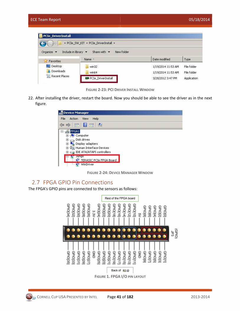
ECE Team Report 05/18/2014
CORNELL CUP USA PRESENTED BY INTEL Page 41 of 182 2013-2014
FIGURE 2-23: PCI DRIVER INSTALL WINDOW
22. After installing the driver, restart the board. Now you should be able to see the driver as in the next
figure.
FIGURE 2-24: DEVICE MANAGER WINDOW
FPGA GPIO Pin Connections The FPGA's GPIO pins are connected to the sensors as follows:
FIGURE 1. FPGA I/O PIN LAYOUT

ECE Team Report 05/18/2014
CORNELL CUP USA PRESENTED BY INTEL Page 42 of 182 2013-2014
Inventory
GPIO Pin Number Purpose
10 Inventory output - OUT
11 Inventory select bit 0 - S0 (least significant bit)
12 Inventory select bit 1 - S1
13 Inventory select bit 2 - S2
14 Inventory select bit 3 - S3
15 Inventory select bit 4 - S4 (most significant bit)
TABLE 2-4: INVENTORY I/O PINS
Ultrasonic Sensors
Pin Number Purpose
1 Right leg low ultrasonic sensor
2 Right leg middle ultrasonic sensor
3 Right leg high ultrasonic sensor
4 Left leg low ultrasonic sensor
5 Left leg middle ultrasonic sensor
6 Left leg high ultrasonic sensor
7 Center low ultrasonic sensor
8 Center middle ultrasonic sensor
9 Center high ultrasonic sensor
TABLE 2-5: ULTRASONIC SENSOR I/O PINS
Note: "Left" and "right" above refer to R2-I2's left and right.
R2-I2 ultrasonic sensor layout is shown in the figure below. Sensor labels in Figure 2-25 correspond to
FPGA I/O pins from Table 2-5.
FIGURE 2-25: ULTRASONIC SENSOR LAYOUT ON R2-I2

ECE Team Report 05/18/2014
CORNELL CUP USA PRESENTED BY INTEL Page 43 of 182 2013-2014
Final Ultrasonic Sensor Implementation using FPGA With reference to the PWM input discussed in Section 2.3.1, we have implemented 9 ultrasonic sensors
using FPGA. These 9 ultrasonic sensors are grouped into 3 sets of 3 sensors each. A single set consists of
3 sensors which are implemented in a daisy chain to avoid prevent interference between the sensors.
Daisy chaining means that the 3 sensors are looped as a ring, wherein the first ultrasonic sensor finds the
range and triggers the next one and so on. In Section 2.3.1 we checked the PWM input for 1 of these
sensors. Now we just have to loop it for 3 sensors and pass it on to Atom via PCIe.
In section 2.3.1 we mentioned that the duty cycle is actually a percentage value. In PWM mode, the sensor
output pin outputs a pulse width representation of the distance with a scale factor of 1us per mm. The
period of the PWM signal is about 100ms. Since the maximum range is 5m, the maximum duty cycle is
5000μ s
0.1s= 5%
The distance equation for the sensor is shown below:
𝐷𝑖𝑠𝑡𝑎𝑛𝑐𝑒 =𝐷𝑢𝑡𝑦 𝐶𝑦𝑐𝑙𝑒
5∗ 5m
The ultrasonic sensors are range finder, so we have a range of values in percentage (duty cycle) not 0 and
1. Hence, to improve obstacle detection we need high accuracy in the readings. In section 2.3.1, we used
below equation to calculate the duty cycle.
𝐷𝑢𝑡𝑦 𝐶𝑦𝑐𝑙𝑒 =𝑑𝑐𝑜𝑢𝑛𝑡𝑒𝑟∗100
𝑝𝑐𝑜𝑢𝑛𝑡𝑒𝑟1
In consideration of implementation complexity and hardware resources, we didn’t add point calculation
unit to our hardware, which will constrain the accuracy of the result value. Thus we made some changes
to equation the Duty Cycle equation, resulting in the equation below.
𝐷𝑢𝑡𝑦 𝐶𝑦𝑐𝑙𝑒(100 𝑡𝑖𝑚𝑒𝑠) =𝑑𝑐𝑜𝑢𝑛𝑡𝑒𝑟 ∗ 10000
𝑝𝑐𝑜𝑢𝑛𝑡𝑒𝑟1
Since the period of the PWM signal is about 100ms for the ultrasonic sensor we used, the maximum high
level voltage signal length is 100𝑚𝑠 ∗ 5% = 5𝑚𝑠. And due to the fact that we used a 50MHz clock to
trigger 𝑑𝑐𝑜𝑢𝑛𝑡𝑒𝑟, the maximum value of 𝑑𝑐𝑜𝑢𝑛𝑡𝑒𝑟 is 5𝑚𝑠
(1/50𝑀𝐻𝑧)= 250000. Therefore, the maximum value
of 𝑑𝑐𝑜𝑢𝑛𝑡𝑒𝑟 ∗ 10000 is 2500000000. By using a 32 bit binary number, the maximum value we can denote
is 232 − 1 = 4294967296 > 2500000000, which means that the way we used to calculate will not cause
any overflow.
Finally, we can use a C++ program on ATOM side to calculate the real distance.
𝐷𝑖𝑠𝑡𝑎𝑛𝑐𝑒 =𝐷𝑢𝑡𝑦 𝐶𝑦𝑐𝑙𝑒(100 𝑡𝑖𝑚𝑒𝑠)
500∗ 5m
The final distance value is later used to perform further calculations. The accuracy is 5𝑚 ∗0.01%
5%= 1𝑐𝑚,
which satisfies the requirements from CS team.
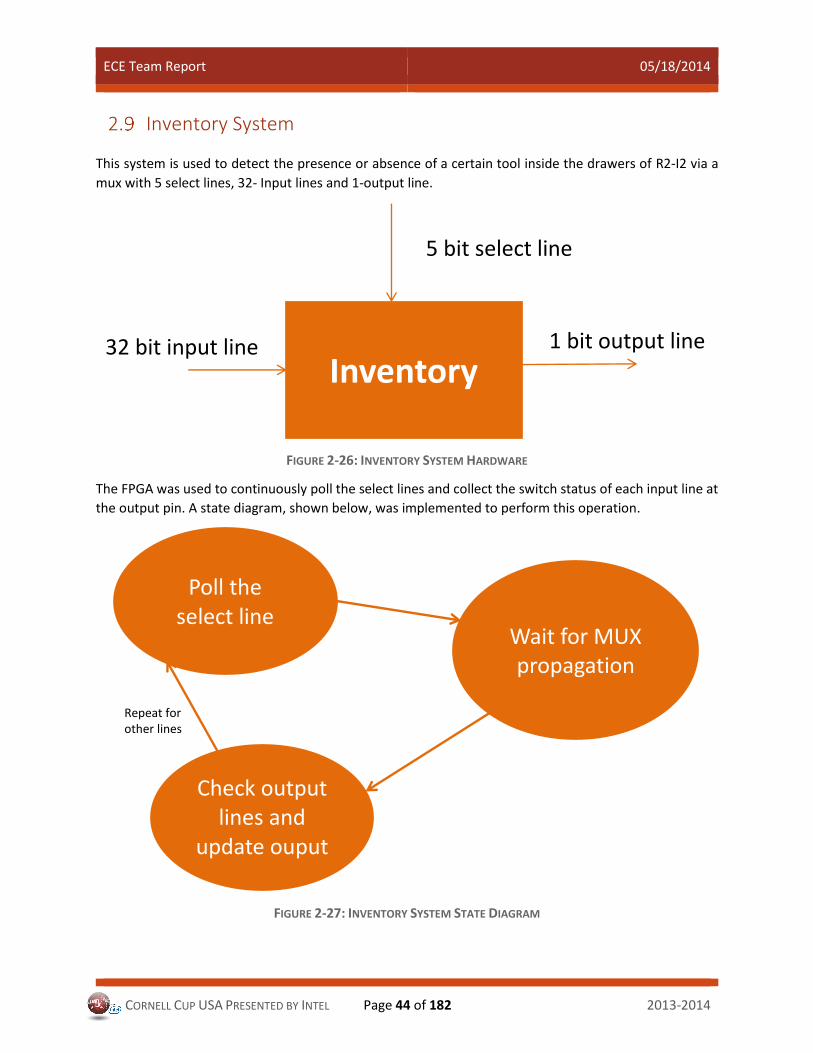
ECE Team Report 05/18/2014
CORNELL CUP USA PRESENTED BY INTEL Page 44 of 182 2013-2014
Inventory System This system is used to detect the presence or absence of a certain tool inside the drawers of R2-I2 via a
mux with 5 select lines, 32- Input lines and 1-output line.
FIGURE 2-26: INVENTORY SYSTEM HARDWARE
The FPGA was used to continuously poll the select lines and collect the switch status of each input line at
the output pin. A state diagram, shown below, was implemented to perform this operation.
FIGURE 2-27: INVENTORY SYSTEM STATE DIAGRAM
Inventory
5 bit select line
32 bit input line 1 bit output line
Poll the select line
Wait for MUX propagation
Check output lines and
update ouput register
Repeat for other lines
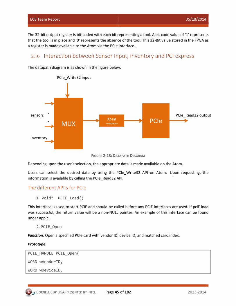
ECE Team Report 05/18/2014
CORNELL CUP USA PRESENTED BY INTEL Page 45 of 182 2013-2014
The 32-bit output register is bit-coded with each bit representing a tool. A bit code value of ‘1’ represents
that the tool is in place and ‘0’ represents the absence of the tool. This 32-Bit value stored in the FPGA as
a register is made available to the Atom via the PCIe interface.
Interaction between Sensor Input, Inventory and PCI express
The datapath diagram is as shown in the figure below.
FIGURE 2-28: DATAPATH DIAGRAM
Depending upon the user’s selection, the appropriate data is made available on the Atom.
Users can select the desired data by using the PCIe_Write32 API on Atom. Upon requesting, the
information is available by calling the PCIe_Read32 API.
The different API’s for PCIe
1. void* PCIE_Load()
This interface is used to start PCIE and should be called before any PCIE interfaces are used. If pciE load
was successful, the return value will be a non-NULL pointer. An example of this interface can be found
under app.c.
2. PCIE_Open
Function: Open a specified PCIe card with vendor ID, device ID, and matched card index.
Prototype:
PCIE_HANDLE PCIE_Open(
WORD wVendorID,
WORD wDeviceID,
MUX
.
. 32-bit register PCIe
PCIe_Read32 output sensors
Inventory
PCIe_Write32 input

ECE Team Report 05/18/2014
CORNELL CUP USA PRESENTED BY INTEL Page 46 of 182 2013-2014
WORD wCardIndex);
Parameters:
wVendorID: Specify the desired vendor ID. A zero value means to ignore the vendor ID.
wDeviceID: Specify the desired device ID. A zero value means to ignore the device ID.
wCardIndex: Note, these three parameters are ignored in Linux edition..
Return Value:
Return a handle to presents specified PCIe card. A positive value is return if the PCIe card is opened
successfully. A value zero means failed to connect the target PCIe card.
Here our wVendorID = DEFAULT_PCIE_VID = 0x1172,
wDeviceID = DEFAULT_PCIE_DID = 0xE001,
wCardIndex = 0
3. PCIE_Write32: The information can be requested from the FPGA using the Write32 interface.
Function: Write a 32-bits data to the FPGA Board.
Prototype:
bool PCIE_Write32(
PCIE_HANDLE hPCIE,
PCIE_BAR PcieBar,
PCIE_ADDRESS PcieAddress,
DWORD dwData);
Parameters:
hPCIE: A PCIe handle return by PCIE_Open function, in our code hPCIe
PcieBar:Specify the target BAR.= DEMO_PCIE_USER_BAR = 0
PcieAddress: Specify the target address in FPGA = 0x00
dwData: Specify a 32-bits data which will be written to FPGA board. This should be the information that
is requested from the FPGA. A table is shown below.
Value of dwData Selection made
1 Sensor - 1
2 Sensor - 2
3 Sensor - 3
4 Sensor - 4
5 Sensor - 5

ECE Team Report 05/18/2014
CORNELL CUP USA PRESENTED BY INTEL Page 47 of 182 2013-2014
6 Sensor - 6
7 Sensor - 7
8 Sensor - 8
9 Sensor - 9
10 Inventory data
FIGURE 2-29: WRITE32 DWDATA TABLE
Return Value: Return TRUE if write data is successful; otherwise FALSE is returned.
4. PCIE_Read32: The information after requesting data from the FPGA can be read by using
Read32 interfaces.
Function: Read a 32-bits data from the FPGA board.
Prototype:
bool PCIE_Read32(
PCIE_HANDLE hPCIE,
PCIE_BAR PcieBar,
PCIE_ADDRESS PcieAddress,
DWORD * pdwData);
Parameters:
hPCIE: A PCIe handle return by PCIE_Open function. = hPCIE
PcieBar: Specify the target BAR.= 0
PcieAddress: Specify the target address in FPGA. = 0x20
pdwData: A buffer to retrieve the 32-bits data. Information where the data is available.
Value of dwData Selection made
1 Sensor - 1 : Duty Cycle of PWM * 100 :Divide the value by 100 to get the Duty cycle in the range of 0 to 100 %
2 Sensor - 2 : Duty Cycle of PWM * 100 : Divide the value by 100 to get the Duty cycle in the range of 0 to 100 %
3 Sensor - 3 :Duty Cycle of PWM * 100 : Divide the value by 100 to get the Duty cycle in the range of 0 to 100 %
4 Sensor - 4 :Duty Cycle of PWM * 100 : Divide the value by 100 to get the Duty cycle in the range of 0 to 100 %
5 Sensor - 5 :Duty Cycle of PWM * 100 : Divide the value by 100 to get the Duty cycle in the range of 0 to 100 %
6 Sensor - 6 :Duty Cycle of PWM * 100: Divide the value by 100 to get the Duty cycle in the range of 0 to 100 %
7 Sensor - 7 :Duty Cycle of PWM * 100: Divide the value by 100 to get the Duty cycle in the range of 0 to 100 %

ECE Team Report 05/18/2014
CORNELL CUP USA PRESENTED BY INTEL Page 48 of 182 2013-2014
8 Sensor - 8 :Duty Cycle of PWM * 100 : Divide the value by 100 to get the Duty cycle in the range of 0 to 100 %
9 Sensor - 9 : Duty Cycle of PWM * 100: Divide the value by 100 to get the Duty cycle in the range of 0 to 100 %
10 Inventory data: 32- Bit inventory system which gives 32-bit coded data.
FIGURE 2-30: READ32 DWDATA TABLE
Return Value: Return TRUE if read data is successful; otherwise FALSE is returned.
5. After all the PCIe communication is completed for ever, close the PCIE handler using
PCIE_Close(hPCIE);
PCIE_Unload(lib_handle); // lib_handle is the address returned by PCIE_Load
3 Sensor Design and Implementation Sensors are used in robots and other autonomous systems to obtain data from external stimuli, which
makes them important if the robots are to interact with the environment. Because sensors play an
important role in gathering external data, their placement is important.
In our design for R2-I2 we needed to determine the functions we wanted it to perform. Knowing these
functions was important because they would determine what sensors we would have to use. For example,
we wanted R2-I2 to be able to avoid bumping objects, therefore we would have to use some sort of sensor
to fulfill the role of detecting objects. The team wrote out all the possible use case scenarios and functions,
and then researched different types of sensors that could get the job done. We then reviewed the list
with the other teams and eliminated some options while finalizing others.
There are three main functionality groups for R2-I2's sensor subsystem: Obstacle Detection, Localization,
and Inventory. These functionality groups then helped us search for specific sensors that would be used
in each case. For each functionality group, we further divided the group into smaller tasks that individual
sensors might be well-suited for. For example, Obstacle Detection was split into smaller tasks like
Detecting Walls and Detecting Edges/Cliffs. Some sensors, like LIDAR, are well-suited for wall detection,
but not the best option for detecting cliffs. From these small tasks, we were able to research and rate
many different sensors according to their usefulness, price, and engineering challenge. These results of
those ratings for the sensors we chose to implement are available in the sensor summary chart in section
3.6.8.
This document also covers our design steps for each functionality group, and the prototyping methods we
used to prepare for implementation. The actual sensors we selected are presented along with sources
and a summary of their specifications. Finally, we discuss the ongoing process of communicating
effectively with other teams and concepts for future features.
Sensor Overview The main objective for R2-I2 is to be an autonomous roving tool chest. This means that it should be able
to move itself around our somewhat cluttered lab without bumping into anything, as well as allow lab

ECE Team Report 05/18/2014
CORNELL CUP USA PRESENTED BY INTEL Page 49 of 182 2013-2014
members to access a set of tools contained within. We also want R2-I2 to track and display which tools
it's currently holding, and keep track of which users were the last to check out any tools that are missing.
This section provides a general overview of the different sensor systems R2-I2 uses, the process used to
select them, and the roles that they fill in achieving our goals.
3.1.1 Sensor Subsystem Requirements The first step in tackling the sensor subsystem problem is developing an understanding of the
requirements the subsystem is expected to fulfill. In comparison to other subsystems within the electrical
engineering team, such as power supply, the sensor requirements are largely self-defined and do not
depend quite so heavily on the needs of other subsystems, aside from the navigation computer science
team. After developing a good understanding of the overall design goals, and receiving the go ahead from
the navigation team, we were in good shape to begin brainstorming the essential demands on our
subsystem. For this early step in the project, we did not commit to one particular sensor or approach, but
instead focused on the overall needs our subsystem has to fulfill. From our discussions, we settled on the
following needs:
3.1.1.1 Obstacle Detection To navigate effectively, R2-I2will need to detect and avoid a wide range of obstacles, including walls,
tables, chairs, humans, wires, bags, trash cans, cliff/stair/stage edges, and more. To avoid obstacles, we
need sensors that can detect objects of varying heights and sizes both in front of and to the sides of R2-
I2. The outputs of these sensors must be something that is readable by either an FPGA board or an Atom
board (see Section Error! Reference source not found., written by our FPGA subteam, for more
information on these) so that these boards can use the data to compute R2-I2's actions. Overall, obstacle
detection is a critical priority for R2-I2, and responsibility for it falls primarily with the sensor subsystem.
3.1.1.2 Localization R2-I2 should have some way of taking in information that allows it to compute where in the area it is. The
information received through these sensors should be readable by an interface board and should contain
enough information to find the robot's location and to create a map of its surroundings. This is a distinct
need from obstacle detection. Determining north/south orientation, for example, is purely a localization
problem. Localization can sometimes be approached with creative solutions, such as detecting the
strength of Wi-Fi signals emanating from known locations, or visually detecting unique patterns placed in
known locations of the lab, or using sensors to build a comprehensive map of the area. Localization is key
to large-scale navigation, such as recognizing a valid destination and planning a path, while obstacle
detection focuses on temporary or smaller obstacles. Of course, many sensors can play a role in both
obstacle detection and localization and mapping, and our localization approach incorporates information
obtained by a wide variety of our sensors. For a more detailed explanation of localization methods, review
documentation by the CS team on their approaches to the problem.
3.1.1.3 Inventory In order to fulfill its tool chest role, R2-I2 should be able to house a set of tools, while keeping track of
which tools are checked out and by whom, as well as which tools are present in the tool chest. The goal
of this inventory check-out system is to maximize access to tools around the lab while minimizing the
number of tools that are lost from the tool chest.

ECE Team Report 05/18/2014
CORNELL CUP USA PRESENTED BY INTEL Page 50 of 182 2013-2014
Obstacle Detection Obstacle detection is a critical feature for R2-I2 because successful navigation is highly dependent on
avoiding obstacles along the path. The goal of obstacle avoidance is first to ensure that R2-I2 does not
get trapped or lose its direction because of an obstacle, and preferably, does not bump into any objects
or walls as it's moving from one location in the lab to another. Obstacle avoidance, meaning the process
the robot follows to determine an alternate route around an obstacle, is relegated to the CS team. But
avoidance is not possible without reliable obstacle detection. Some design aspects we had to consider
were the location of the sensors on R2-I2 and tricky situations R2-I2 might face. For obstacle avoidance
some sensors we decided to investigate were Ultrasonic Rangefinders, a Webcam, an Xbox Kinect,
Thermal Sensors, and LIDAR. These sensors will be discussed in detail below.
3.2.1 Requirements Like when brainstorming the overall requirements of our sensor subsystem, we brainstormed the specific
requirements associated with obstacle detection. This helped us evaluate the usefulness of each sensor.
The following needs were identified:
3.2.1.1 Wall Detection Detecting and avoiding any object that can stop the robot is important, but wall detection is one of the
main concerns. Even in an environment with no other obstacles, R2-I2 will still need to recognize and
avoid driving into a wall. Because walls are wide, flat surfaces, they are fairly easy to detect, and so there
are many sensors that are more or less capable of detecting walls. One of the key measures of good
performance in this area is finding an approach that will allow the robot to tell the difference between a
wall and another form of obstacle.
3.2.1.2 Small Object Detection (under 12' high) Small object detection is both very important and very difficult. Small objects are capable of severely
interfering with R2-I2's movement, potentially causing damage to the system, or getting crushed or
damaged by R2-I2 itself. All of these outcomes are obviously undesirable. But small objects can also be
very difficult to detect, and the difference between dangerous small objects (feet, rocks) and irrelevant
small objects (dropped pieces of paper, pencils, dust bunnies, etc.) can be very for sensors to evaluate.
With high stakes and high difficulty, we are very interested in finding a reliable solution to this problem.
3.2.1.3 Large Object Detection (over 12' high) Large objection detection poses unique challenges compared to small object and wall detection. Unlike
walls, large objects have a large variety of shapes. Most sensors relying on some form of reflection, like
LIDAR or ultrasonic sensors, might fail to detect the legs of a chair, for instance. Other objects, like tables,
can prevent R2-I2's movements but can be completely undetectable to a sensor at the wrong height. To
ensure reliability in large object detection, the sensors must be able to handle a huge variety of object
shapes.
3.2.1.4 Human Recognition Being able to recognize humans is useful for making R2-I2 entertaining to interact with. For example, if
R2-I2 detects that the object nearby is a human rather than a chair, the robot could interact or "talk" to

ECE Team Report 05/18/2014
CORNELL CUP USA PRESENTED BY INTEL Page 51 of 182 2013-2014
the person. In addition, this part is useful for localization and mapping, because while we want to map
furniture, we do not want to map humans, since they rarely stay in the same place.
3.2.1.5 Cliff Detection The ability to detect cliffs as R2-I2 is moving is important because we want to protect the robot from
accidentally driving off a stair or an edge, which would damage the robot and possibly hurt anything or
anyone who was at the bottom of the edge. For this part, we need to ensure that R2-I2 can reliably detect
when the ground in front of one or more of its sensors has gotten farther away than it normally is. False
positives (falsely assuming that there is a cliff even when there is not) are preferable to false negatives
(wrongly assuming that there is no cliff when there is). The output of this segment must be such that it
can be interpreted fast enough so that a signal to stop can be sent to R2-I2's motion systems.
3.2.2 Design 3.2.2.1 Typical Use Cases Looking at a large variety of possible use cases helps us to anticipate possible weaknesses of proposed
designs, and helps to create more effective designs.
Use Case Desired Response Requirement
R2-I2 approaches cliff or edge in desired path
Immediately stop all locomotion motors
Shall detect all cliffs or edges in direction of motion within maximum stopping distance
R2-I2 approaches a wall in desired path
Turn or stop to avoid hitting wall
Shall detect all walls in direction of motion within maximum stopping distance
R2-I2 approaches a standing human in desired path
Turn or stop to avoid hitting human
Shall detect large (>12' high) soft objects in direction of motion within maximum stopping distance
R2-I2 approaches table in desired path
Turn or stop to avoid hitting table
Shall detect horizontal objects at any height below maximum height of R2-I2
R2-I2 approaches power cable on ground in desired path
Run over cable Shall evaluate height of potential obstacles
Moving human steps in front of moving R2-I2
Minimize impact by stopping all motors
Shall detect large (>12' high) soft objects within range smaller than maximum stopping distance
R2-I2 approaches cardboard box on ground in desired path
Turn or stop to avoid hitting box
Shall detect small (<12' high) hard objects in direction of motion within maximum stopping distance
Idle R2-I2 is approached by human
Issue greeting Shall detect and identify approaching object as human
TABLE 3-1: TYPICAL USE CASES
3.2.2.2 Rejected Implementations We considered using a radar system (see section 3.6.9: Other Sensors Considered) to sense distances to
surrounding objects. However, this system was deemed to be too expensive, and we can get similarly
useful and accurate data from the ultrasonic rangefinders that we chose.

ECE Team Report 05/18/2014
CORNELL CUP USA PRESENTED BY INTEL Page 52 of 182 2013-2014
Another possible method for detecting obstacles would be to use a regular video camera. However, this
set-up would actually only give us a 2-dimensional representation of what is around R2-I2, so we would
not get any useful information about the distances to those objects.
3.2.2.3 Final Design The sensors we decided to use for the scenarios mentioned above are the ultrasonic range finder, LIDAR,
webcam and Kinect. Each sensor has a specific task and will fulfill the requirements that are needed by
the design. Of course the scenarios mentioned in 3.1.1 are much harder to implement than they may
seem. We realize that to properly get a working scenario we have to think of the many possibilities that
could happen in each scenario. The coding of the logic will be handled by the CS team.
Each sensor has a part in the scenarios described in 3.1.1. The roles of these sensors are described below.
The ultrasonic sensor is used to detect objects within a range and to then trigger next logical responses.
The robot’s response depends on which ultrasonic sensor is triggered. For example, if the ultrasonic sensor
that is responsible for edge detection is triggered, the command to stop the robot is sent out. However,
if it is the ultrasonic sensor for object detection, a command to check whether the object is human or not
is sent out.
The LIDAR sensor is one that maps out a room and can help with localization (see section 3.3: Localization)
but also detection of objects as R2-I2 moves around in the lab. It works like a radar and helps detect
objects. One of the many uses of LIDAR is mapping out the structure of objects. For example, the LIDAR
has the ability to map out a chair or table with its legs. This can help us identify objects as R2-I2 moves
around in the lab. Implementation of the LIDAR has been left to the CS team because it is a plug and play
device and thus the information goes straight to a computer or base station.
The Webcam and Kinect are also plug and play devices and their programming has been left to the CS
team. However, we had to plan the use case scenarios and therefore we recognized their use in object
detection. The Kinect will be used to detect humans while the webcam will be used to detect objects for
localization (see section 3.3: Localization) and object detection. The Kinect will be used for gestures and
is very handy because of the amount of work done on it by Microsoft and other vendors (it is suggested
to find and read about the use of Kinect in the CS documentation).
3.2.3 Prototyping In this section we discuss testing the ultrasonic sensor using the Arduino Mega microcontroller. The
purpose was to test logic and fulfil proof of concepts outlined in earlier sections of this document. To
connect to the ultrasonic rangefinder, connect to the pins as follows.
Pins Used:
PIN 2 - Pulse Width Representation of Analog Output
Frequency: 10Hz, Period: 100ms
HIGH: Vdd, LOW: 0
Width: 1 microsecond per 1 mm of range
PIN 4 - Turnoff Input

ECE Team Report 05/18/2014
CORNELL CUP USA PRESENTED BY INTEL Page 53 of 182 2013-2014
Apply HIGH (Vdd) voltage to this pin to turn off sensor and output will be constant 0.
PIN 6 - Vdd
Operates between 2.5V and 5.5V
Try to run at around 5V for best results; you’ll get a larger range.
PIN 7 - GND
FIGURE 3-1: MULTIPLE SENSOR OPERATION
3.2.3.1 Arduino Set-up Rangefinder Connected to the Arduino Mega along with the IMU:

ECE Team Report 05/18/2014
CORNELL CUP USA PRESENTED BY INTEL Page 54 of 182 2013-2014
FIGURE 3-2: ARDUINO MEGA WITH RANGEFINDER
When reading from the rangefinder using an Arduino, there are a few things to consider when choosing
which data pin to reference, such as how the rangefinder will ultimately interface with your robot, and
the accuracy of the data type.
We decided to use the PWM data pin of the rangefinder (pin 2) to connect to the Arduino because we
ultimately planned to interface the rangefinder with the DE2 FPGA board, and on the DE2 board it is
simpler to work with PWM signals than Analog signals because it does not require ADC. Also, PWM signals
are used to drive servos, which we also control from the FPGA, so it was the natural choice here (See
section 2.3 about PWM on the FPGA board).
When programming the Arduino Mega to read the Rangefinder PWM data line, there are a few things to
keep in mind (reference the figure below to see our source code as you read along):
Be sure to define your output baud rate and any constants you want (i.e. #define
CONSTANT_NAME constant).
Be sure to declare and assign each pin used on the microcontroller and internal variables.
Any function or loop or setup you define needs to be declared with a return type and wrapped in
{} brackets.
Always use void setup() {stuff} to initialize everything that you don't need to update
constantly. It will run before anything else regardless of its position in the code. This is where you
define what pins are outputs and what pins are inputs. This is also where you define any initial
output values or volatile variables.
Always use a void loop() {function}, which runs directly after the setup() to run a function
that defines the value at your output pins.

ECE Team Report 05/18/2014
CORNELL CUP USA PRESENTED BY INTEL Page 55 of 182 2013-2014
FIGURE 3-3: RANGE FINDER CODE

ECE Team Report 05/18/2014
CORNELL CUP USA PRESENTED BY INTEL Page 56 of 182 2013-2014
3.2.4 Testing Results and Sensor Selection There are a wide variety of small, relatively inexpensive ultrasonic sensors available. After finishing our
prototype with one ultrasonic sensor and an Arduino, it became much easier to test a variety of sensors
to find the best ones for our purposes.
We tested ultrasonic sensors from Maxbotix’s LV-ProxSonar®-EZ™ and HRLV-ProxSonar®-EZ™ sensor line.
These sensors cost between $20 and $40 each and are easily available by ordering from the Maxbotix
website. These sensors were designed to be used in protected, indoor environments, but outdoor
ultrasonic sensors are also available. Each line offers individual products with detection zones on a scale
from 0 to 4. The 0 sensors have the widest detection zone, while the 4’s have the most narrowly focused.
We were interested in testing a variety in order to determine which is most appropriate for our purposes.
To test, we slightly modified the prototype design seen above to have much longer wires. This allowed us
to arrange the sensor with a great deal of freedom. We then taped the sensor to a position on R2-I2’s
frame that we were considering for use. From there, we watched its output as we placed various objects
in and just outside of its field of view. These objects, as described above, included walls, small objects,
large objects, and people. We then taped the floor to note the edge of the ultrasonic’s detection zone.
We repeated this process for each sensor from 0 to 4 and for each mounting position we were considering
for use.
From our tests, we found the HRLV-EZ2 and the HRLV-EZ4 to be the most promising. The HRLV line differs
from the LV line in that the HRLV is a much higher level of resolution, with 1 mm resolution instead of 1
inch resolution. The HRLV also offers superior noise rejection. We were able to see this in our testing.
Unfortunately neither the HRLV nor the LV offered perfectly stable readings. Even in a stable position with
unmoving objects, the readings from both types fluctuated from one reading to another. Still, the HR line
was found to have less fluctuation than the LV line, another reason why it was chosen. As for the HRLV-
EZ2 specifically, we found it had a detection zone about 2 feet across, while the other sensors had
detection zones slightly wider or narrower. Because R2-I2 is two feet wide, this made the HRLV-EZ2 the
perfect fit for forward-facing sensors to detect all possible obstacles with a minimal chance of interference
from objects R2-I2 is not on a path to collide with. The HRLV-EZ4 has a much narrower detection zone,
the narrowest offered by Maxbotix. This made it ideal for sensors mounted on the left or right edge of R2-
I2, in order to minimize false positives.
3.2.4.1 Detailed Use Cases for Position Decision After testing each ultrasonic sensor, we made decisions regarding the positioning of the sensors on R2-I2
in order to fulfill the system requirements discussed earlier. To do this, we created a detailed list of use
cases for likely objects that R2-I2 will need to respond to. We also created a list of possible sensor
locations. Together, this formed a matrix describing which sensor position is capable of serving us for each
use case. This also helped us to determine which sensors would be needed, and how many of each. Finally,
this document serves to aid the CS team in interpreting ultrasonic sensor data, as each sensor’s purpose
is well defined through this matrix.

ECE Team Report 05/18/2014
CORNELL CUP USA PRESENTED BY INTEL Page 57 of 182 2013-2014
FIGURE 3-4: SENSOR SELECTION MATRIX
To aid in interpreting this document, an X indicates the sensor is capable of detecting the use case,
whether that means a larger or smaller reading than usual. A ‘ – ‘ indicates that the sensor might be able
to detect the use case sometimes, but not reliably. The columns with red text indicate sensor positions
that, through this analysis, were deemed unnecessary and were no longer evaluated beyond this point.
Rows with red highlighted backgrounds indicate use cases that functionality is desired in, but which our
design cannot handle. ‘Unambiguous Reading’ determines if the readings from the ultrasonic sensors
allow R2-I2 to unambiguously identify which use case is occurring. The goal of this matrix is to find an
unambiguous reading for each unique expected reaction, so R2-I2’s reaction is always appropriate for the
use case, while using a bare minimum of ultrasonic sensors. The reference numbers in blue correspond
with this diagram of the layout of sensors (sensor 9’s location is approximate, as it had not been installed
when this photo was taken):
Sensor Locations >
Cen
ter, L
ow
, No
inclin
e
Sid
e 1
, Lo
w, N
o in
clin
e
Sid
e 2
, Lo
w, N
o in
clin
e
Cen
ter, L
ow
, Inclin
ed
Up
Sid
e 1
, Lo
w, In
clin
ed
Up
Sid
e 2
, Lo
w, In
clin
ed
Up
Cen
ter, H
igh
, Inclin
ed
Do
wn
Sid
e 1
, Hig
h, In
clin
ed
Ste
ep
ly D
ow
n
Sid
e 2
, Hig
h, In
clin
ed
Ste
ep
ly D
ow
n
Cen
ter, C
en
ter, N
o
inclin
e
Sid
e 1
, Hig
h, In
clin
ed
Do
wn
, An
gle
d S
ligh
tly
Ou
t
Sid
e 2
, Hig
h, In
clin
ed
Do
wn
, An
gle
d S
ligh
tly
Ou
t
Exp
ecte
d R
eactio
n
Un
am
big
uo
us R
ead
ing
?
Ideal Sensor Type HRLV-EZ 2 HRLV-EZ 2 HRLV-EZ 4 HRLV-EZ 4 HRLV-EZ 2 HRLV-EZ 4 HRLV-EZ 4 HRLV-EZ 4 HRLV-EZ 4
Reference Number 7 8 1 4 9 3 6 2 5
Table
round table head on (Front) X -- -- X Stop, find alternate path Yes
rectangular table head on
(Front) X X X X X Stop, find alternate path Yes
table on one side "1" of robot -- X -- Stop, find alternate path Yes
table on one side "2" of robot -- X -- Stop, find alternate path Yes
Wall
wall, head on X X X X X X X X X X X X Stop, find alternate path Yes
wall, headed into corner X X X X X X X X X X X X Stop, find alternate path Yes
doorway/corner, going to clip - - X X X X Adjust Course Maybe
doorway/corner, not going to
clip X X - - X X Continue Course Maybe
Obstacles with varying widths
Chair, head on X X -- -- -- X X Stop, find alternate path Yes
Profile Chair, head on - - - X X X X - Stop, find alternate path Yes
Small Obstacles (ex. Book, Brick)
Head on (Front) X
X(d>6
ft)
X(d>6
ft) X - Stop, find alternate path Yes
Right side X(d > 6 ft) X X Stop, find alternate path Maybe
Left Side X(d > 6 ft) X X Stop, find alternate path Maybe
Turning right towards small,
close object X Stop, find alternate path Yes
Turning leftt towards small,
close object X Stop, find alternate path Yes
Right side, will not clip X - Continue Course Maybe
Left side, will not clip X - Continue Course Maybe
Moving Obstacles
Foot steps into path of side 1
wheel X X - - Stop, find alternate path Yes
Foot steps into path of side 2
wheel X X - - Stop, find alternate path Yes
Cliff
Cliff, head on X X X Stop, find alternate path Yes
U-shaped cliff X X X Stop, find alternate path Yes
Skinny gap, head on Stop, find alternate path NO
Skinny gap, at angle Stop, find alternate path NO
Driving parallel to cliff - - X X Stop, find alternate path Yes

ECE Team Report 05/18/2014
CORNELL CUP USA PRESENTED BY INTEL Page 58 of 182 2013-2014
FIGURE 3-5: PLACEMENT OF ULTRASONIC SENSORS
3.2.5 Ultrasonic Sensor Implementation Once the type and positioning of each sensor was determined, it became time to actually install the
sensors. To minimize interference, the 9 sensors were daisy-chained in 3-chain segments. This means that
all sensors on the left leg fire in sequence, which prevents their readings from interfering with each other.
This is also true for the right leg, and all three sensors in the center. Daisy-chaining is desirable because it
can eliminate interference from other ultrasonics. We decided to use three separate daisy chains both to
provide resiliency if one sensor fails to function or is missing, and to reduce the excessive amount of wire
that would be required to chain 9 sensors to one location. Instructions for wiring an ultrasonic sensor
daisy chain were provided by Maxbotix and are available in the prototyping section of this document. We
chose to implement the constantly looping method:

ECE Team Report 05/18/2014
CORNELL CUP USA PRESENTED BY INTEL Page 59 of 182 2013-2014
FIGURE 3-6: CONTINUOUS DAISY-CHAIN DIAGRAM BY MAXBOTIX
The 9 sensors are controlled by the FPGA. The loop can be initially triggered by Pin 4, which activates the
first sensor. The loop will then continue indefinitely. Because we chose to use three separate daisy chains
of 3 sensors each, the FPGA needs to trigger three different sensors to begin all three loops.
FIGURE 3-7: ULTRASONIC SENSOR PINOUT
We utilized pins 2 and 4 for this setup. Pin 2 outputs a PWM (pulse width modification) signal which can
be read to determine the sensor’s reading. PWM is a way of sending data where the pin is set to high for
a portion of a set cycle time. In the case of these sensors, every 𝜇S the pin is high corresponds to an
additional mm of distance, up to a maximum of 5000 mm (about 16 feet). These sensors can also be read
using analog or serial outputs, using pins 3 and 5 respectively. The PWM is actually 0.5% less accurate
than the other methods of receiving the data, and in cases where accuracy is extremely important, it
should be avoided in favor of analog or serial. For our purposes, high levels of accuracy weren’t critical
and our FPGA team preferred using PWM.
Pin 4 triggers the sensor to take a reading. When held continuously high, the sensor will continuously take
readings. When low, the sensor will not take readings. Cleverly, Maxbotix recommends using PWM output
(which is low for long periods of time, then is high for a short duration immediately after a reading) as a
trigger for the next sensor in the daisy-chain. The data can be read, but it can also be used as a way of
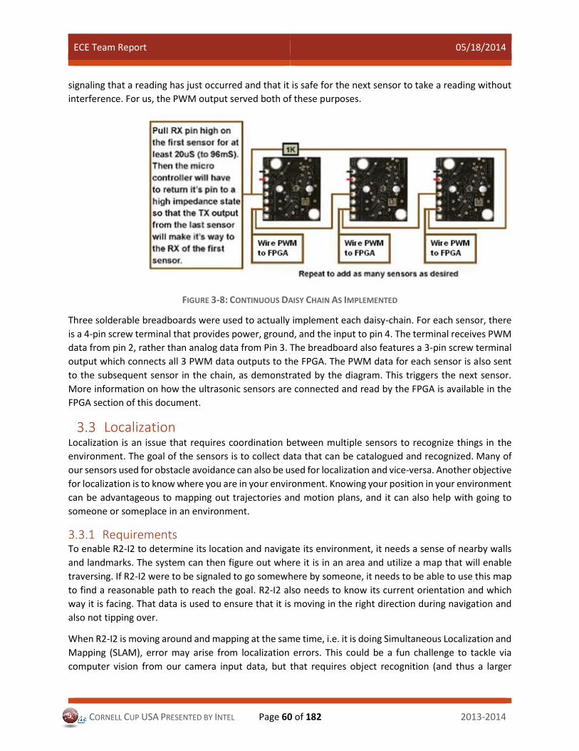
ECE Team Report 05/18/2014
CORNELL CUP USA PRESENTED BY INTEL Page 60 of 182 2013-2014
signaling that a reading has just occurred and that it is safe for the next sensor to take a reading without
interference. For us, the PWM output served both of these purposes.
FIGURE 3-8: CONTINUOUS DAISY CHAIN AS IMPLEMENTED
Three solderable breadboards were used to actually implement each daisy-chain. For each sensor, there
is a 4-pin screw terminal that provides power, ground, and the input to pin 4. The terminal receives PWM
data from pin 2, rather than analog data from Pin 3. The breadboard also features a 3-pin screw terminal
output which connects all 3 PWM data outputs to the FPGA. The PWM data for each sensor is also sent
to the subsequent sensor in the chain, as demonstrated by the diagram. This triggers the next sensor.
More information on how the ultrasonic sensors are connected and read by the FPGA is available in the
FPGA section of this document.
Localization Localization is an issue that requires coordination between multiple sensors to recognize things in the
environment. The goal of the sensors is to collect data that can be catalogued and recognized. Many of
our sensors used for obstacle avoidance can also be used for localization and vice-versa. Another objective
for localization is to know where you are in your environment. Knowing your position in your environment
can be advantageous to mapping out trajectories and motion plans, and it can also help with going to
someone or someplace in an environment.
3.3.1 Requirements To enable R2-I2 to determine its location and navigate its environment, it needs a sense of nearby walls
and landmarks. The system can then figure out where it is in an area and utilize a map that will enable
traversing. If R2-I2 were to be signaled to go somewhere by someone, it needs to be able to use this map
to find a reasonable path to reach the goal. R2-I2 also needs to know its current orientation and which
way it is facing. That data is used to ensure that it is moving in the right direction during navigation and
also not tipping over.
When R2-I2 is moving around and mapping at the same time, i.e. it is doing Simultaneous Localization and
Mapping (SLAM), error may arise from localization errors. This could be a fun challenge to tackle via
computer vision from our camera input data, but that requires object recognition (and thus a larger

ECE Team Report 05/18/2014
CORNELL CUP USA PRESENTED BY INTEL Page 61 of 182 2013-2014
database to reference), kinematics calculations, and accurate mapping—so it is worthwhile to implement
simpler localization methods. For example, GPS localization is a commonly used technique for outdoor
robotic systems. However, for our purposes, a 9 axis IMU will do the trick—which basically gives yaw,
pitch, roll, and directional acceleration measurements (for more, see section 3.6: Sensor Selection).
3.3.1.1 Orientation R2-I2 needs to be able to reference itself in some axes of orientation. This data can come from sensors
that act as idiothetic sources for R2-I2. Idiothetic sources give information about the absolute position of
the system, e.g. the direction of a compass's needle would tell us where the robot is pointing. Something
to take note of is that idiothetic sensors are prone to cumulative error over time because of a myriad of
reasons, such as random vibrations from the system and output data rounding, so several idiothetic
sensors must be used to keep each other in check and accurately measure orientation.
For orientation, the system needs to be able to gather sensor data for the most commonly referenced XYZ
axes. This is used as odometry data i.e. the velocity and position of the system while it is moving or staying
still. The sensors have to output data quick and accurate enough to perform dead reckoning methods
where its current position is calculated by using a previously determined position, and advancing that
position based upon estimated speed and direction over elapsed time.
Yaw, pitch, and roll are also useful axes to gather data about to reference the system's complete 3-
dimensional orientation in space. This data ensures R2-I2 is correctly localized in the map and also works
as a fail-safe for cautions like tipping over.
3.3.1.2 Mapping R2-I2 also needs to have an idea of where its system is in an environment. Thus it needs to be able to
sense and detect nearby walls and obstacles because these landmarks can be used as references in a map.
Once our system knows where it is in a known map or floor plan, it can calculate the shortest path,
avoiding obstacles, from its current position to any endpoint. We would only need one allothetic source,
i.e. a sensor that takes in information about the surrounding environment, which is fast and accurate
enough to sense and recognize the obstacles and walls around it. Other sensors could be used in
simultaneously for obstacle detection and map learning, such as a thermal sensor which would
differentiate between a human and an inanimate object.
3.3.2 Design 3.3.2.1 Typical Use Cases Brainstorming a list of use cases helps us to determine which sensor implementations will effectively
meet the requirements of the project.
Use Case Desired Response Requirement
R2-I2 sent to identified location on known map
R2-I2 plans path between current location to destination
Shall determine current location and orientation in known environment
R2-I2 sent to identified location in unfamiliar area
R2-I2 explores and maps possible paths to destination
Shall generate map of major obstacles along path between two locations in unknown environment

ECE Team Report 05/18/2014
CORNELL CUP USA PRESENTED BY INTEL Page 62 of 182 2013-2014
R2-I2 detects unmapped obstacle
Determines if object should be mapped as permanent obstacle
Shall determine if object appears permanent or not
TABLE 3-2: LOCALIZATION USE CASES
3.3.2.2 Rejected Implementations We considered using a GPS system for finding R2-I2's location. However, GPS does not work well indoors
because of the signal interference that comes from going through walls and ceilings. In addition, the level
of accuracy that we would require for GPS would be very expensive. The GPS would need to stay very still,
as little vibrations can throw off the readings. We also left the thermal sensor for future iterations, in favor
of focusing our efforts on more important functions.
3.3.3 Implementation 3.3.3.1 Idiothetic Sensors for Absolute Position Many robotic systems use an inertial measurement unit (IMU) as its main localization sensor. An IMU can
report its own position and velocity using a combination of sensors consisting of an accelerometer, a
gyroscope, and a magnetometer. These sensors report back real-time data about the sensor's position in
a six axes plane. Previously calculated position data can be used in conjunction with current data to
calculate velocity and acceleration data, in a technique called dead reckoning. Unfortunately, despite the
relatively high accuracy of the IMU data for calculating current position, any error from each
measurement, no matter how small, accumulates into drift over time. This error grows exponentially and
has to be accounted for.
Originally, we had considered putting our IMU velocity data through a closed-loop filter that would take
in previous IMU data outputs as feedback to minimize the drift. However, the high complexity of
implementing these filtering techniques and their relative ineffectiveness in accounting for drift forced us
to seek an alternative solution. We decided to add more idiothetic sensors along with the IMU to
collaboratively calculate R2-I2's position and keep each other's drift in check.
These other sensors do not have to be as accurate as the main IMU to help out with R2-I2's absolute
position calculation. Optical sensors and rotary encoders were two sensors we looked at that used a
similar dead reckoning technique for calculating velocity based on previously calculated position data.
Optical sensors localize the system the same way our optical computer mice figure out where our cursor
is - velocity is calculated based on where the laser was last shot out of and later detected. Rotary encoders,
which conveniently come with the motors ordered, localize the system by looking at which ways the
motors have moved and how quickly they moved.
The IMU model selected for this project was the “9 Degrees of Freedom – Sensor Stick (IMU)”. See section
3.8.7 for more information. This model was selected simply because of its low cost and small size. Its
sensor output was accurate and sensitive to orientation changing, so it served our purposes well.
3.3.3.1.1 HOOKING IT UP
To use this IMU sensor on our robotic system, we connected it to a microcontroller on an Arduino MEGA
board. The microcontroller processes and reads orientation data from the IMU through an I2C
connection. The microcontroller and IMU are bolted onto the robot, so they move along with the
robot. Thus, we get accurate orientation data from the robot.

ECE Team Report 05/18/2014
CORNELL CUP USA PRESENTED BY INTEL Page 63 of 182 2013-2014
FIGURE 3-9: IMU SETUP
The electrical connection of the sensor requires 4 connections: a 5V power line which we connected
straight to the 5V line on the microcontroller powered by the USB power hub, a ground line which we
arbitrarily connected to any of the grounds on the system, and the two SDA/SCL connection pins which
we hooked up to the corresponding pins on the microcontroller board so that there could be a connection
between the two systems. The sensor output is conveniently sent through serial communication, and can
be read through a serial monitor like Putty.exe (see Inventory section for setup instructions).
3.3.3.1.2 ARDUINO CODE
The code that we used was an open source example code found on GitHub. We modified the code so that
instead of constantly outputting the data through the serial line, the system would create a buffer of data
that contains all of the required yaw, pitch, and roll data in a specific format that can be parsed on the
Atom board. The code can be found here: https://github.com/ptrbrtz/razor-9dof-ahrs and in the Google
Drive.
3.3.3.1.3 MAGNETIC FIELD CONCERNS
For the IMU to output accurate data, specifically from the magnetometer, the magnetic field needs to be
constant or else the data will be corrupted. We tested out different scenarios with different magnetic
fields such as those from smartphones, computers, and high power motors to find out the proximity of
the changing magnetic field before it starts affecting the sensor. This range is taken into account when we
decided the placement of the sensor in the whole system, as we placed the IMU at the bottom center of
R2-I2 near the FPGA, away from all the motors which, when accelerating, modify the surrounding
magnetic field.
3.3.3.2 Allothetic Sensor for Territory Exploration A common technique used by robotic systems to detect and analyze their nearby surroundings is Light
Detection And Ranging (LiDAR). LiDAR is an allothetic sensor that shoots and receives a laser to calculate
distance from the obstacles that the laser bounces off of. We found a low-cost LiDAR sensor that scans a

ECE Team Report 05/18/2014
CORNELL CUP USA PRESENTED BY INTEL Page 64 of 182 2013-2014
360 degree view quick enough, even when R2-I2 is moving, and robustly maps out walls and obstacles.
We make use of its detection abilities to reference nearby objects to known maps and localize R2-I2 in
familiar surroundings. Additionally, in an unknown environment, the LiDAR sensor can work with other
object detection sensors to create a map for R2-I2 while it is exploring the area.
The LiDAR sensor uses a simple plug-and-play interface through USB and the data is readily available when
the system is powered. After applying it to our use case scenarios, we handed the sensor over to the CS
Team.
Inventory The purpose of R2-I2's tool chest is to increase accessibility to tools in the lab. This goal is achieved by
keeping all of the frequently used tools in one easy-to-find location (R2-I2's chest) and by minimizing the
number of tools that are lost from the chest.
3.4.1 Requirements To minimize the number of lost tools, we decided to use a check-out system. Such a system would
discourage users from losing or leaving tools out of the R2-I2's tool chest. This system would require two
steps: 1) identifying users who want to check out tools, and 2) sensing which tools are present and which
are absent from the tool chest.
3.4.1.1 User Identification This step requires uniquely identifying users who want to check out a tool from R2-I2's chest so that we
can keep track of who has checked out which tools. User identification could also be used to ensure that
only authorized users can open the tool chest.
The user identification system must be simple and quick to use, so as not to interrupt the flow of work of
whoever is using it.
A sensor in this step would need to output a unique identifier or signal for each different user. The output
signal must also be readable by a board or computer so that the information can be stored.
3.4.1.2 Inventory The inventory system must be able to relay the state of the tool chest to an interface board or computer.
To accomplish this, there must be some mechanism for sensing which tools are present in the chest and
which are absent.
This system should be robust and not prone to errors. It also should not rely heavily on users removing or
replacing tools in a "just right" way. We want usage of the inventory system to be as seamless as possible.
The sensors in this step should output a signal that accurately conveys the state of the tool chest. The
signal has to have enough information to tell us whether each tool is present or absent, and the signal has
to be readable by some interface board so that it can be interpreted there.
3.4.2 Design 3.4.2.1 Typical Use Cases Table 1-1 shows a list of the inventory system’s typical use cases and the behavior that we aimed to
achieve.

ECE Team Report 05/18/2014
CORNELL CUP USA PRESENTED BY INTEL Page 65 of 182 2013-2014
Use Case Desired Response Requirement
A user wants to know the location of a tool
R2-I2 visually indicates tool location
Shall know location of carried tools
A user removes a tool R2-I2 tracks that tool is missing
Shall detect when tool is present or missing
A user attempts to return tool to incorrect location
R2-I2 refuses to accept improperly placed tool
Shall determine or prevent incorrect tool placement
A user identifies him/herself to check out tool(s)
R2-I2 associates user with removed tools
Shall identify users uniquely and track tool removal
A user attempts to remove tool without identification
R2-I2 indicates unauthorized access
Shall detect and record unauthorized access
A user identifies self to return tool(s)
R2-I2 identifies tools returned with user
Shall identify users uniquely and track tool return
R2-I2 is commanded to move while drawer is open
R2-I2 refuses to move Shall detect when drawer is open and prevent locomotion
TABLE 3-3: INVENTORY USE CASES
3.4.2.2 Rejected Implementations User Identification:
Each user is assigned a unique number which they can enter into a keypad on the robot as
identification. This method was rejected because users might forget their identification numbers
and waste time trying to remember the numbers or just give up trying to use R2-I2's tool chest at
all.
Inventory:
Each tool has a small RFID (radio-frequency identification) tag mounted on it, and an RFID reader
would tell the robot's computer which tools are present based on which RFID tags are present.
This method of inventory was rejected because most RFID readers can only read one RFID tag at
a time. If more than one tag is within reading range of the reader, then either only one or neither
of the tags will be read.
For each tool, one small button is wired into the bottom of the tool chest. In order to ensure that
tools get placed on the buttons and with enough downward force on the buttons, a clasp is
mounted around the button with the proper width of the tool. This method was rejected because
it requires assembling extra parts with a certain amount of precision and because it would require
extra effort from the user.
3.4.2.3 Final Design User Identification:
Our system uses an RFID reader to identify users. Each person who has access to the tool chest
will receive an RFID card that holds a unique binary number. When a user wants to access the
tool chest, he or she taps the RFID card against an RFID reader that is attached to the robot.
This method is advantageous because it requires little extra effort from the user. A possible
drawback is losing ID cards, but this is easily avoided if ID cards are properly kept.

ECE Team Report 05/18/2014
CORNELL CUP USA PRESENTED BY INTEL Page 66 of 182 2013-2014
Inventory:
To keep track of inventory, we use snap-action switches mounted at the bottom of each tool
drawer. Snap-action switches are small and require little force to activate (between 25 and 150
grams). However, this means that we cannot use this system to track tools under 25 grams.
In order to ensure that tools get returned to their proper switches, a foam cut-out of each tool is
be placed over that tool's respective switch. Having cut-outs of each tool also makes it harder for
the user to miss the switch when returning a tool, yet it requires little effort from the user to do
so.
3.4.2.4 Future Designs The following designs are being considered for future iterations of the inventory system:
Lock the drawers on R2-I2 until a user scans his or her identification card. Once the card is
scanned, an electrical system would unlock the desired tool chest. This feature was considered
for future designs because at the moment it seems unnecessary and cumbersome, since most
users in the lab can be trusted to identify themselves before opening the tool chest. Such a
system would also involve wiring extra electrical systems, requiring additional time and creating
additional failure.
Disallow R2-I2 from moving while the tool chest is open. Such a feature would detect if any of
the three tool drawers are open and send a signal to an interface board if so. This would help
ensure the safety of those around the robot, as having R2-I2 move while its drawers are open
could cause tools to fall out. It would also encourage users to fully close each drawer when they
are done checking tools in and out.
3.4.3 Prototyping 3.4.3.1 Part Selection Please refer to section 3.63.6 for details and links to the parts used for the RFID system. We decided to
use an RFID system that came pre-assembled from Sparkfun, because we know little about the ins-and-
outs of how RFID works, so buying a system that was ready to use out of the box saved us time and
heartache. Buying from Sparkfun was also advantageous because their website contains a tutorial for
setting up and using the RFID reader. (See section 3.4.3.2 below for the tutorial.) In addition, the RFID
reader that we selected connects to a computer via USB and outputs information using RS232 serial. This
kind of output is perfect for reading through any serial console on a computer, which means that we can
bypass the FPGA and transmit data straight to the Atom board on the robot.
For the inventory switches, we decided to use an array of snap-action switches. Our prototype uses
switches from Omron’s D2F series (datasheet). The termination style on these switches makes them useful
for prototyping. We considered two types of switches: low-force and standard force. Low-force snap-
action switches require only 25 grams to activate (press down), while standard force switches require 80
grams to activate. For prototyping and testing, we ordered both of these types of switches.
In addition to the array of inventory switches, we had a set of multiplexers so that we could limit the
number of input and output pins needed on the FPGA. Without these multiplexers, each tool in the tool
chest would require its own input pin on the FPGA. By using multiplexers, we avoid having many wires

ECE Team Report 05/18/2014
CORNELL CUP USA PRESENTED BY INTEL Page 67 of 182 2013-2014
going into the FPGA, which is messy and hard to keep track of. The size of the multiplexers that we choose
will also help determine how many tools we will allow in the tool chest. The downside of this setup,
however, is that we need to assemble the multiplexers, and these additional connections become
additional points of possible failure. For the prototype, we chose to use three 8:1 multiplexers (datasheet)
fed into a 4:1 multiplexer (datasheet). Both of these parts are manufactured by Texas Instruments.
3.4.3.2 Setup of RFID System Setting up and using the RFID reader: A tutorial for using the RFID reader can be found on Sparkfun’s
website (for Windows XP). The tutorial also describes some of the hardware of the RFID reader.
Other parts needed:
RFID Reader from Sparkfun (the lab currently has the RFID Reader ID-20LA, but other readers with
shorter range are also available).
RFID tags that use EM4001 RFID protocol (three types are available on Sparkfun).
Mini-USB type-B cable (we have several in the Cornell Cup Lab).
Windows computer with a USB port.
The schematic for the reader is located here: RFID USB Reader schematic. Note that there are pins that
can be used for reading serial data, if USB-serial connection is not wanted.
If using Windows XP, drivers can be downloaded at this link: FTDI virtual COM port drivers.
For Windows 7, follow the instructions of the Sparkfun tutorial with the following changes:
1. No need to download drivers, as instructed in the tutorial -- drivers will be automatically
installed.
2. Download PuTTY as your serial console (no installation required).
3. In the Device Manager, under Ports (COM & LTP), note at which COM port the reader (called
"USB Serial Port") is.
4. Open PuTTY by running putty.exe.
a. Under Connection type, select Serial.
b. In the left sidebar, select Connection → Serial.
c. Under "Select a serial line", enter COMxx, where xx is the number of the COM port
found in step 3.
d. Check that the remaining fields match the fields in the tutorial (shown below).

ECE Team Report 05/18/2014
CORNELL CUP USA PRESENTED BY INTEL Page 68 of 182 2013-2014
FIGURE 3-10: COMXX PROPERTIES
e. If desired, save the session settings in PuTTY.
f. Click Open. If the COM port is connected and correct, a new PuTTY session should open.
5. No need to click any buttons to start the session (as described in the Sparkfun tutorial). Just place
an RFID tag near the reader.
6. Once an RFID tag is placed within three or four inches of the reader, the tag's unique 32-bit ID will
be read and printed in hexadecimal notation on the serial console.
3.4.3.3 Block Diagram of Inventory System Figure 3.11 shows a block diagram of how the various components of the inventory system interact.
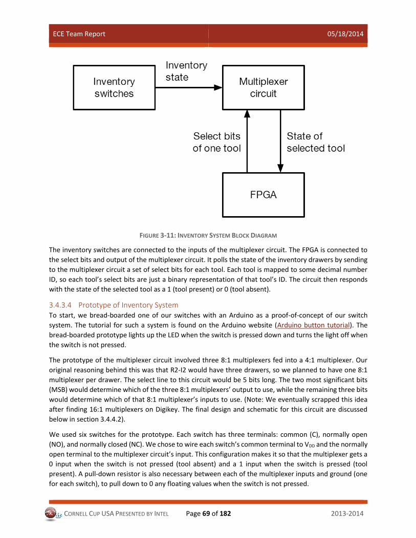
ECE Team Report 05/18/2014
CORNELL CUP USA PRESENTED BY INTEL Page 69 of 182 2013-2014
FIGURE 3-11: INVENTORY SYSTEM BLOCK DIAGRAM
The inventory switches are connected to the inputs of the multiplexer circuit. The FPGA is connected to
the select bits and output of the multiplexer circuit. It polls the state of the inventory drawers by sending
to the multiplexer circuit a set of select bits for each tool. Each tool is mapped to some decimal number
ID, so each tool’s select bits are just a binary representation of that tool’s ID. The circuit then responds
with the state of the selected tool as a 1 (tool present) or 0 (tool absent).
3.4.3.4 Prototype of Inventory System To start, we bread-boarded one of our switches with an Arduino as a proof-of-concept of our switch
system. The tutorial for such a system is found on the Arduino website (Arduino button tutorial). The
bread-boarded prototype lights up the LED when the switch is pressed down and turns the light off when
the switch is not pressed.
The prototype of the multiplexer circuit involved three 8:1 multiplexers fed into a 4:1 multiplexer. Our
original reasoning behind this was that R2-I2 would have three drawers, so we planned to have one 8:1
multiplexer per drawer. The select line to this circuit would be 5 bits long. The two most significant bits
(MSB) would determine which of the three 8:1 multiplexers’ output to use, while the remaining three bits
would determine which of that 8:1 multiplexer’s inputs to use. (Note: We eventually scrapped this idea
after finding 16:1 multiplexers on Digikey. The final design and schematic for this circuit are discussed
below in section 3.4.4.2).
We used six switches for the prototype. Each switch has three terminals: common (C), normally open
(NO), and normally closed (NC). We chose to wire each switch’s common terminal to VDD and the normally
open terminal to the multiplexer circuit’s input. This configuration makes it so that the multiplexer gets a
0 input when the switch is not pressed (tool absent) and a 1 input when the switch is pressed (tool
present). A pull-down resistor is also necessary between each of the multiplexer inputs and ground (one
for each switch), to pull down to 0 any floating values when the switch is not pressed.

ECE Team Report 05/18/2014
CORNELL CUP USA PRESENTED BY INTEL Page 70 of 182 2013-2014
3.4.4 Implementation 3.4.4.1 Final Part Selection The final implementation of the RFID reader, as far as sensors go, is detailed above in the Prototyping
section (section 3.4.3). Instructions for setting up serial communication between the reader and a
computer are also described in that section.
For the final implementation, we decided to use snap-action switches manufactured by Omron (part
number: SS-01GL-E– datasheet). We chose these switches because they have a low (8 g) operating force
(i.e., pressing force required before the switch clicks into place) and because the solder lug terminals make
it easy to wire up the switches to the robot.
The multiplexers that we decided on for the final circuit are 16:1 multiplexers from Texas Instruments
(part number: CD74HC4067E – datasheet). We used two 16:1 multiplexers because we hoped for the tool
chest to be able to hold around 30 tools. This means 32 inputs and thus 5 select bits (S0 to S4).
Since there are only two multiplexers, we use the ICs’ enable bits plus an inverter to choose between the
two. We feed the select bits’ MSB (S4) directly to the multiplexer governed by switches 0 to 15 (mux 1),
and feed the MSB inverted (~S4) to the multiplexer governed by switches 16 to 31 (mux 2). Since the
enable bit is active low, mux 1’s output will be used when S4 is 0, and mux 2’s output will be used when
S4 is 1.
Each input to the multiplexers needs to be connected to a pull-down resistor to zero out any floating
values when the switches are open. To avoid needing 32 separate resistors, we used five resistor
networks, each with 8 resistors (part number: 4116R-1-RC – datasheet).
Lastly, to aid in connecting the switches’ wires to the board, we used five 8-pin screw terminals,
manufactured by Molex (part number: 39357-0008 – datasheet).
The multiplexers, inverter, resistor networks, and screw terminals make up R2-I2’s inventory board.
3.4.4.2 Circuit Diagram of Inventory Board The final schematic of the inventory system is shown below. U1 and U2 are the 16:1 multiplexers, and U7
is the inverter that aids in selecting between the two multiplexers. U3 through U6 are resistor networks
Note that each input (S0 through S4 and SW0 through SW31) is connected to a pull-down resistor. These
inputs, as well as the VDD rail on the right of the schematic, are connected as screw terminals.

ECE Team Report 05/18/2014
CORNELL CUP USA PRESENTED BY INTEL Page 71 of 182 2013-2014
FIGURE 3-12: INVENTORY SYSTEM CIRCUIT DIAGRAM

ECE Team Report 05/18/2014
CORNELL CUP USA PRESENTED BY INTEL Page 72 of 182 2013-2014
3.4.4.3 PCB Design An illustration of the inventory board is shown below. The labels on each part correspond to the labels in
the schematic above.
FIGURE 3-13: INVENTORY SYSTEM PCB
3.4.4.4 Connecting the Inventory Switches Each switch has two wires coming out of it: one wire is connected to VDD and the other to its respective
connector (one of SW0 through SW31 in Figure 3-13 above). The switches are wired as shown below. We
soldered each wire to the switch terminals and then covered the terminals and exposed wire with heat
shrink.
FIGURE 3-14: SWITCH WIRING

ECE Team Report 05/18/2014
CORNELL CUP USA PRESENTED BY INTEL Page 73 of 182 2013-2014
Sensor Precedence This section will be devoted to discuss scenarios that require interaction between sensor subsystems and
require more thought and planning as well as those scenarios that do not have any obvious programming
logic. Below is a list of such scenarios brainstormed that require a sensor-based solution. Each of these
problems was considered during both the determination of sensors to use, and the placement of the
sensors on the bot. Furthermore, we must focus on implementing solutions that give proper priority to
the correct subsystem. Many of these solutions may be implemented through other teams, such as the
CS team, but it is our responsibility to anticipate possible conflicts our subsystem might be involved in
ahead of time, to better coordinate the system's response among competing subsystems.
3.5.1 Use Case Scenarios that do not involve people The scenarios considered are listed below:
R2-I2 is in a corner, leading to conflicting responses from different wall sensors.
R2-I2 runs into something it cannot roll over or something that is should not roll over, leading to
a lack of movement but no obvious object detection.
R2-I2 is in a situation that causes tilt, threatening damage without object detection.
R2-I2 cannot turn or move because the wheels are stuck, leading to lack of movement but no clear
object detection.
R2-I2 is given a destination which is impossible to reach without passing through a detected
object, leading to conflict between navigation goals and object detection and avoidance goals.
R2-I2 is surrounded by many obstacles, and must reverse.
3.5.2 Use case Scenarios that involve people In this section we will discuss scenarios that R2-I2 might encounter that involve people.
The scenarios are listed below:
R2-I2 is being called on by a lab member and on his way is interrupted by another lab member
who wants a tool, leading to conflict between navigation goals and the inventory subsystem.
R2-I2 is set to follow or approach a certain team member or person, leading to conflict between
navigation goals and obstacle detection and avoidance goals of avoiding people.
Sensor Selection When selecting sensors, it is important to consider their specs and determine if they meet your
requirements. Depending on the application, the best sensor may or may not be obvious. After compiling
a list of requirements and the use case scenarios for those requirements, we have a comprehensive idea
of the tasks our sensors need to accomplish. We can then rate each possible sensor according to how well
it accomplishes our needs.
List of Sensors Cornell Cup USA presented by Intel Decided to use:

ECE Team Report 05/18/2014
CORNELL CUP USA PRESENTED BY INTEL Page 74 of 182 2013-2014
3.6.1 RFID USB Reader
Cost: $24.95
Model: SEN-09963
images are CC BY-NC-SA 3.0
FIGURE 3-15: SEN-09963
Description: The RFID USB Reader is a simple to use, USB to serial base unit for the ID-3LA, ID-12LA, and
ID-20LA readers. Simply plug a reader into the headers and attach a mini-USB cable. Open a terminal
program of your choice at 9600bps 8N1, then scan your 125kHz ID tag and the unique 32-bit ID will be
shown on the screen. The unit is based on a FTDI chip and comes with a read LED and buzzer.
This new revision uses SMD headers for the RFID module, and has a solder jumper which allows you to
disable or enable the buzzer.
Note: This product does not come with the RFID reader. Check below for compatible readers.
Dimensions: 1.4x1.2x0.57"
Documents:
Schematic
Eagle Files
Tutorial
USB FTDI Drivers for Linux, MAC, and PC

ECE Team Report 05/18/2014
CORNELL CUP USA PRESENTED BY INTEL Page 75 of 182 2013-2014
3.6.2 RFID Reader ID-20LA (125 kHz)
Cost: $34.95
Model: SEN-11828
images are CC BY-NC-SA 3.0
FIGURE 3-16: SEN-11828
Description: RFID (radio-frequency identification) is the wireless non-contact use of radio-frequency
electromagnetic fields, for the purposes of identifying and tracking tags attached to objects. This is the ID-
20LA, a very simple to use RFID reader module from ID Innovations. With a built in antenna, the only
holdup is the 2mm pin spacing (breakout board available below). Power the module, hold up a 125kHz
card, and get a serial string output containing the unique ID of the card.
The new ID-20LA is essentially the same as the older ID-20, but has a lower input voltage.
Features:
2.8 - 5V supply
125kHz read frequency
EM4001 64-bit RFID tag compatible
9600bps TTL and RS232 output
Magnetic stripe emulation output
Read range of 180mm
Dimensions: 38x40x7mm
Documents:
Datasheet
Bildr Tutorial

ECE Team Report 05/18/2014
CORNELL CUP USA PRESENTED BY INTEL Page 76 of 182 2013-2014
3.6.3 RFID Tag (125kHz)
Cost: $1.95
Model: COM-08310
images are CC BY-NC-SA 3.0
FIGURE 3-17: COM-08310
Description: RFID is useful for sensing and identifying tagged people and objects for access control,
automation, and a whole range of different applications. This basic RFID tag works in the 125kHz RF range
and comes with a unique 32-bit ID. It is not re-programmable. This blank, smooth, and mildly flexible RFID
tag is ready for your logo (or hand-drawn scribble).
Dimensions: 2.13 x 3.35 x 0.03" (54 x 85.5 x 0.8mm)
Features:
EM4001 ISO based RFID IC
125kHz Carrier
2kbps ASK
Manchester encoding
32-bit unique ID
64-bit data stream [Header+ID+Data+Parity]
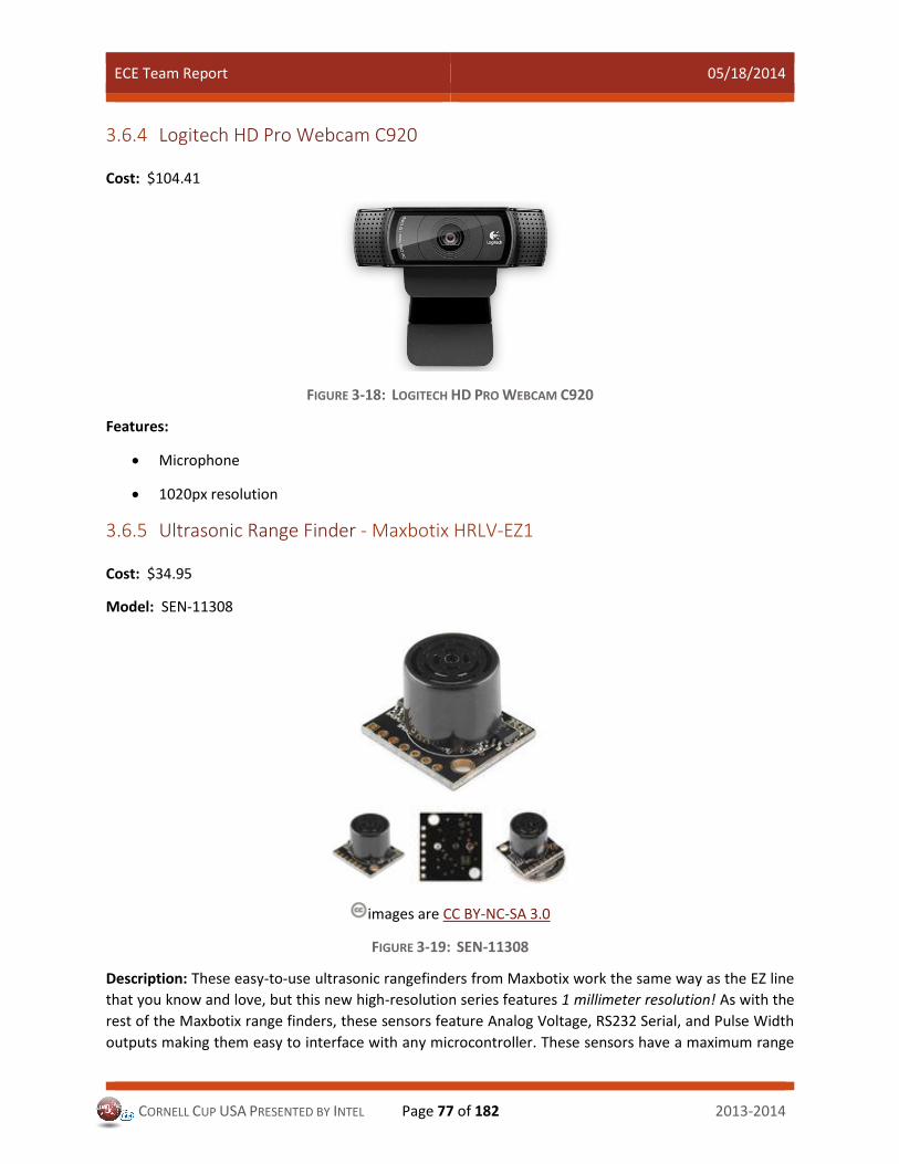
ECE Team Report 05/18/2014
CORNELL CUP USA PRESENTED BY INTEL Page 77 of 182 2013-2014
3.6.4 Logitech HD Pro Webcam C920
Cost: $104.41
FIGURE 3-18: LOGITECH HD PRO WEBCAM C920
Features:
Microphone
1020px resolution
3.6.5 Ultrasonic Range Finder - Maxbotix HRLV-EZ1
Cost: $34.95
Model: SEN-11308
images are CC BY-NC-SA 3.0
FIGURE 3-19: SEN-11308
Description: These easy-to-use ultrasonic rangefinders from Maxbotix work the same way as the EZ line
that you know and love, but this new high-resolution series features 1 millimeter resolution! As with the
rest of the Maxbotix range finders, these sensors feature Analog Voltage, RS232 Serial, and Pulse Width
outputs making them easy to interface with any microcontroller. These sensors have a maximum range

ECE Team Report 05/18/2014
CORNELL CUP USA PRESENTED BY INTEL Page 78 of 182 2013-2014
of 5000 mm (195 inches) with virtually no dead zone (although objects closer than 30 cm will typically
range as 30 cm).
We're offering the EZ0, EZ1, and EZ4 with progressively narrower beam angles allowing the sensor to
match the application. Please see beam width explanation below.
Control up to 10 sensors with only two pins! Checkout the Maxbotix FAQ listed below.
Features:
42kHz Ultrasonic sensor
Operates from 2.5-5.5V
Low 3.1mA average current requirement
10Hz reading rate
Analog Voltage, RS232 or TTL Serial, and Pulse Width
Small, lightweight module
Documents:
Datasheet
Beam Width Explanation
Maxbotix FAQ
3.6.6 New Neato Xv-11 LiDAR Laser Distance Sensor
Cost: $100
FIGURE 3-20: NEATO XV11
Documents:
Description
Demo
Specs

ECE Team Report 05/18/2014
CORNELL CUP USA PRESENTED BY INTEL Page 79 of 182 2013-2014
HowTo
Github
3.6.7 9 Degrees of Freedom - Sensor Stick (IMU)
Cost: $99.95
Model: SEN-10724
images are CC BY-NC-SA 3.0
FIGURE 3-21: SEN-10724
Description: The 9DOF Sensor stick is a very small sensor board with 9 degrees of freedom. It includes
the ADXL345 accelerometer, the HMC5883L magnetometer, and the ITG-3200 MEMS gyro. The 'stick'
has a simple I2C interface and a mounting hole for attaching it to your project. Also, the board is a mere
0.036" thick (0.093" overall), allowing it to be easily mounted in just about any application.
Having a hard time picking an IMU? Our Accelerometer, Gyro, and IMU Buying Guide might help!
Dimensions: 1.37x0.42"
Documents:
Schematic
Eagle Files
Datasheet (ADXL345)
Datasheet (HMC5883L)
Datasheet (ITG-3200)
AHRS/Head-tracker Tutorial
3.6.8 Sensor Summary Chart

FUNCTION SUBFUNCTION
RFI
D
Feat
her
Swit
ches
Ult
raso
nic
Ran
gefi
nd
er
Kin
ect
LID
AR
Cam
/Mic
Bu
mp
Sen
sor
IMU
Ther
mal
IR
Arr
ay
Tab
let
Wif
i Re
ceiv
ers`
Object Detection
Wall Detection 2 3 3 1 2
Small Object Detection(under 12'
high)
2 2 1 1 2
Large Object Detection(over 12'
high)
2 3 1 1 2
Human Recognition 1 3 1 1 3
Cliff Detection 3 1
Localization
Orientation 1 1 2 2 3 2
Mapping 1 3 3 1 1 1
Object Inventory
Identifying Users 3
Inventory 2 3
Receiving Commands
Verbal Commands 2 2
Gesture Commands 3 1
Digital Signal 3 3
Price 1 1 2 1 1 1 0 1 1 3 0
Engineering Difficulty 0 1 2 2 3 3 1 0 2 0 1

ECE Team Report 05/18/2014
CORNELL CUP USA PRESENTED BY INTEL Page 81 of 182 2013-2014
Score Subsystem Rating Price Rating Engineering Difficulty Rating
0 or blank Not Useful Total implementation under $50 Extremely easy to implement complete
solution; plug and play
1 Supplemental usefulness;
Inappropriate as only
solution
Total implementation under $100 Some learning or physical effort required;
may require some soldering, or has a user
interface that must be learned
2 Occasionally useful but in a
limited way
Total implementation under $500 Significant effort required, but the
necessary steps for successful
implementation are understood and
expected to succeed
3 Comprehensively solves the
problem with minor support
Total implementation over $500 Unique solution must be designed,
implemented, and tested, and success is
not guaranteed
TABLE 3-4: SENSOR SUMMARY CHART

ECE Team Report 05/18/2014
CORNELL CUP USA PRESENTED BY INTEL Page 82 of 182 FALL 2013
3.6.9 Other Sensors Considered: 3.6.9.1 RFID Button - 16mm (125kHz)
Cost: $35.60
Model: SEN-09417
images are CC BY-NC-SA 3.0
FIGURE 3-22: SEN- 09417
Description: This is a simple, thumbnail-size RFID tag. These tags are great for sensing presence,
identification, etc., and they're small, so they can be easily sewn into clothing or inserted into enclosures.
Each tag comes with a unique 32-bit ID code and is not reprogrammable. The carrier frequency of this tag
is 125kHz, so it works great with our ID-2, ID-12 and ID-20 RFID readers.
We tested this RFID tag with one of our ID-12 readers and measured a maximum read distance of about
32mm.
Features:
32-bit unique ID - non-reprogrammable
125kHz read frequency
EM4001 ISO based RFID IC
Manchester encoding
Dimensions:
Diameter: 16mm
Thickness: 1.85mm

ECE Team Report 05/18/2014
CORNELL CUP USA PRESENTED BY INTEL Page 83 of 182 FALL 2013
We had originally planned on using these RFID buttons because we thought that we could attach them to
tools and use the RFID reader to keep track of inventory. (See section 3.4.2.2: Rejected Implementations.)
However, the RFID reader cannot read more than one RFID tag at a time, and asking users to tap their
tools in front of an RFID reader before checking in and out tools is unreliable, since it is easy for users to
forget to do this.
3.6.9.2 Radar Demonstration Kit
Cost: $599.99
FIGURE 3-23: RADAR DEMONSTRATION KIT
Key Features
Operates in the International 2.4 GHz ISM Band
Output Frequency Range: 2.4 GHz to 2.5 GHz
Control though USB or Bluetooth
o Android application available now!
Available Radar Modes
o CW
o FMCW
o Doppler
Available Output Waveforms
o Single Tone
o Frequency Ramp

ECE Team Report 05/18/2014
CORNELL CUP USA PRESENTED BY INTEL Page 84 of 182 FALL 2013
o Sawtooth
USB Powered from your computer or optional USB Battery Pack
Mounting platform with Tripod mount available
On-board speaker to listen to the received waveform (after downconversion)
Signal strength meter
Use preset filtering or add your own in the filter prototyping area
We decided not to use this sensor despite its user-friendly interface because the sensor from Sparkfun
(mentioned earlier in this section) gives data that is just as good and has the advantage of daisy chaining
capabilities without interference! In other words, the Sparkfun sensor can be chained to other like
rangefinders so one sensor does not interfere with the others. Another reason we rejected this sensor is
that it is expensive, and we could get just as accurate information from the ultrasonic sensors that we
selected.
3.6.9.3 Devantech SRF05 Ultrasonic Range Finder
Cost: $27.95
FIGURE 3-24: DEVANTECH SRF05
Features:
• Ranges from 1cm to 4m
• Returns a positive TTL level signal, width proportional to range
• 3-4cm Resolution
• Dimensions: 43mm x 20mm x 17mm
The Devantech Ultrasonic Range Finder SRF05 allows you to determine the exact distance of an obstacle
in the sonar field of view. The cleverness of your robot will depend on a sensitive sensor similar to the one

ECE Team Report 05/18/2014
CORNELL CUP USA PRESENTED BY INTEL Page 85 of 182 FALL 2013
bats use to know their position and track prey. With advanced programming, you can design
compensators in order to perfectly control your motors according to the obstacle's distance.
We decided to use the MaxBotix rangefinder instead of this model because it had a higher maximum
range for around the same cost. Additionally, this rangefinder model uses both a sonar output and a sonar
input while the MaxBotix rangefinder uses one sonar for both input and output. Using separate sonar
input and output is more computationally intensive because it requires a pin to switch between input and
output and the switch would be triggered by an interrupt, which requires more code.
Interfacing In this section we will talk about how we collaborated with other teams, what teams we collaborated
with, and what our roles were in the respective teams.
3.7.1 Mechanical Engineering Team We needed to collaborate with the mechanical engineering team because we needed to know the
dimensions of R2-I2, as well as general information on weight, estimated stopping distance and top speed.
Specifically, many of the object detection requirements depend on these mechanical facts. By knowing
these values, we can figure out where to place the sensors so that they will have the best effect. Knowing
R2-I2's size and weight also helped us to estimate the robot's stopping distance so that we could select
the most effective rangefinders. Furthermore, since the Mech-E team will be the primary users of the
tools that are part of the inventory system, we needed to know their requirements for designing a useful
and useable system.
Sensors affected:
Ultrasonic rangefinders
Inventory switches
Xbox Kinect
Webcam
IMU
3.7.2 FPGA Sub-team Among the Electrical Engineering sub-teams that we worked with, the FPGA team was the one with which
we had to collaborate the most, because a lot of sensor data is sent to the CS team via the FPGA or Atom
board. We therefore had to make sure that the outputs of our sensors are in formats that the FPGA team
can use and interpret. We discussed the sensors we wanted before purchasing to ensure that the sensor
output would be usable by the FPGA team, and this was an important guiding factor in some of our
purchasing decisions.
Sensors affected:
Ultrasonic sensor
Inventory switches

ECE Team Report 05/18/2014
CORNELL CUP USA PRESENTED BY INTEL Page 86 of 182 FALL 2013
3.7.3 Computer Science Team Computer Science is a department that needs to get data from the sensors to code higher-level logic and
decisions made from sensory inputs. They are also responsible for ensuring communication between
sensors and their base station. Our involvement with CS is to ensure they understand what type of data
they are getting and to ensure they get correct and usable data. We also had to understand what types
of sensory data the CS team needed so that we could obtain and set up systems that could take in such
data.
Sensors affected:
Ultrasonic sensor from the FPGA
Inventory system (via FPGA)
RFID read from the Atom
IMU read from the Atom
Kinect
Webcam
Addendum of Ideas for R2-I2 and I-3P0. R2-I2 should be able to communicate with I-3P0 in the event that someone wants to call R2-I2
from I-3P0.
R2-I2 should be aware of whether its drawer is open, and will not move if it is for safety reasons.
I-3P0 could have microphones in each 'ear', and a pair of headphones could be combined with the
Oculus Rift for greater immersion.
R2-I2 should be able to take in verbal commands and forward that information to an interface
board so that it can be interpreted by voice recognition software (created by the CS team).
R2-I2 should be able to take in video inputs of humans making gestures so that those images can
be forwarded to an interface board and interpreted. The videos that are forwarded have to be of
a good enough quality that the objects in them can be analyzed and identified.
A possible method of summoning R2-I2 would be to make it receive a wireless signal from certain
stations situated around the lab. An advantage of this method would be that we would be able to
pinpoint where the request is coming from based on which station summoned R2-I2. The outputs
have to be readable by some interface board so that they can be interpreted.
3.8.1 Typical Use Cases In this section we will list the ideas that we had of commanding R2-I2 and what sensors would be required
to capture each command.
Commands and their different ways to be relayed to R2-I2 as well as the sensors needed to read the
commands are listed below:
Use Case Desired Response Requirement

ECE Team Report 05/18/2014
CORNELL CUP USA PRESENTED BY INTEL Page 87 of 182 FALL 2013
User issues known voice command
R2-I2 obeys command Shall correctly interpret known voice commands
User issues known physical command
R2-I2 obeys command Shall correctly interpret known physical commands
User summons R2-I2 to base station
R2-I2 obeys summon Shall correctly receive and interpret digital commands at a distance
User commands immediate shutdown
R2-I2 disconnects power to all motors
Shall correctly receive and interpret 'kill switch' command with high reliability
TABLE 3-5: COMMAND RECEIPT USE CASES
These are some ideas that we have that we think are implementable on R2-I2 and are also a basis for
further ideas and work for commanding and controlling R2-I2.
3.8.2 Rejected Implementations We considered the possibility of having an array of microphones mounted around R2-I2, with the idea
that these microphones could help us locate from which direction a command or request was coming. We
rejected this design because it would be difficult to detect where a sound is coming from if there is
significant echo in a room.
4 Power Systems Introduction to v-i transients in electrical circuits
4.1.1 Introduction Voltage and current transients are real problems that need to be considered when designing electrical
circuits. A transient is a temporary spike that occurs in a circuit under a given situation. If left alone,
transients can damage components and break a circuit. In general, transients are generated in many
different situations, but this document will focus on how to deal with ones that may occur on the start-
up condition, and when switching the direction of a motor.
4.1.2 Handling Inrush Currents An inrush current is an instantaneous current that is drawn by a circuit when power is first turned on. An
inrush current is a large spike that can be up to one-hundred times larger in magnitude than the steady-
state current. There is no single reason why inrush currents occur; many different devices contribute to
total inrush current. Capacitors are one of these contributors. When first turning on an electrical circuit,
capacitors are normally discharged. In order to properly charge capacitors to steady-state, a current is
needed. Another key contributor to inrush currents are filaments. When filaments are cold, they have a
low resistance, causing a large current to flow. As time passes and these filaments warm up, their
resistance increases, which causes steady-state current to drop. Figure 4-1: Inrush Current Example,
shows a visualization of inrush current1:
1 http://www.murata.com/products/emicon_fun/2012/10/emc_en29.html
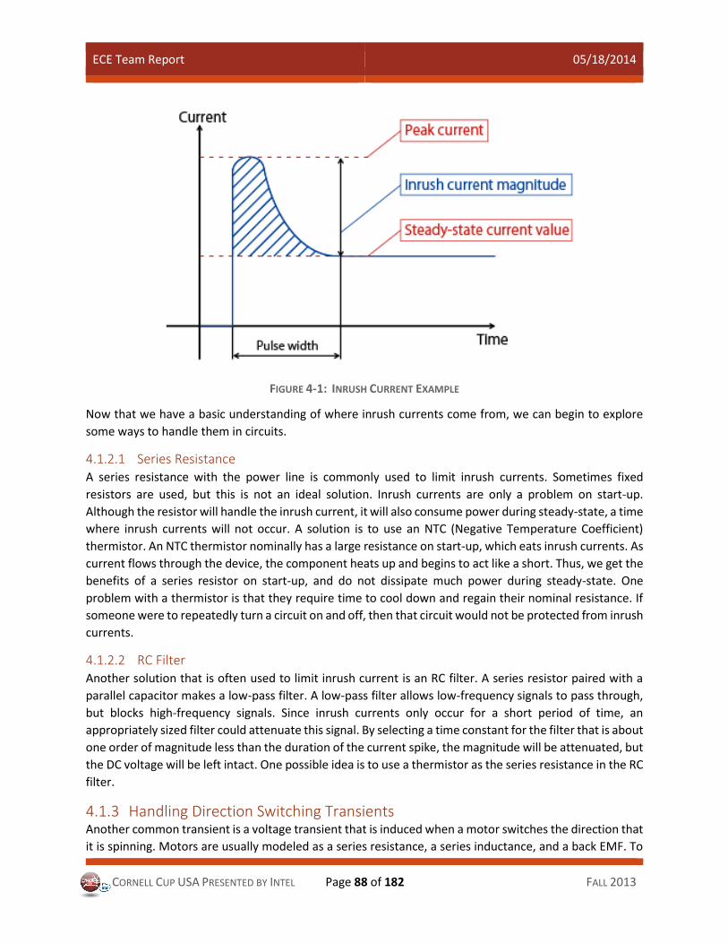
ECE Team Report 05/18/2014
CORNELL CUP USA PRESENTED BY INTEL Page 88 of 182 FALL 2013
FIGURE 4-1: INRUSH CURRENT EXAMPLE
Now that we have a basic understanding of where inrush currents come from, we can begin to explore
some ways to handle them in circuits.
4.1.2.1 Series Resistance A series resistance with the power line is commonly used to limit inrush currents. Sometimes fixed
resistors are used, but this is not an ideal solution. Inrush currents are only a problem on start-up.
Although the resistor will handle the inrush current, it will also consume power during steady-state, a time
where inrush currents will not occur. A solution is to use an NTC (Negative Temperature Coefficient)
thermistor. An NTC thermistor nominally has a large resistance on start-up, which eats inrush currents. As
current flows through the device, the component heats up and begins to act like a short. Thus, we get the
benefits of a series resistor on start-up, and do not dissipate much power during steady-state. One
problem with a thermistor is that they require time to cool down and regain their nominal resistance. If
someone were to repeatedly turn a circuit on and off, then that circuit would not be protected from inrush
currents.
4.1.2.2 RC Filter Another solution that is often used to limit inrush current is an RC filter. A series resistor paired with a
parallel capacitor makes a low-pass filter. A low-pass filter allows low-frequency signals to pass through,
but blocks high-frequency signals. Since inrush currents only occur for a short period of time, an
appropriately sized filter could attenuate this signal. By selecting a time constant for the filter that is about
one order of magnitude less than the duration of the current spike, the magnitude will be attenuated, but
the DC voltage will be left intact. One possible idea is to use a thermistor as the series resistance in the RC
filter.
4.1.3 Handling Direction Switching Transients Another common transient is a voltage transient that is induced when a motor switches the direction that
it is spinning. Motors are usually modeled as a series resistance, a series inductance, and a back EMF. To

ECE Team Report 05/18/2014
CORNELL CUP USA PRESENTED BY INTEL Page 89 of 182 FALL 2013
spin a motor in the forward direction, we apply particular positive voltage to the motor. After a given
duration of time, the motor reaches a steady-state. When a negative voltage is applied across the motor
to switch directions, a voltage transient is induced. This is because of the inductor inside of the motor. In
introductory circuit classes, we learn that the voltage across an inductor is modeled by:
𝑉𝐿 =𝐿𝑑𝐼
𝑑𝑡
When we take away the voltage that is driving the motor to stop the robot, or apply a negative voltage to
make the robot go in reverse, we generate a large change in current in the inductor. This large “𝑑𝐼” over
a short “𝑑𝑡” induces a large voltage transient. If left alone, this large transient can cause some serious
damage to our circuits. We will now present some hardware and software solutions to deal with inductive
kickback generated by motors.
4.1.3.1 Overspec Components One possible solution to handle motor voltage transients is to just deal with it and select beefy
components. For example, we could just select large MOSFETs for the H-bridge that is most likely driving
the motor, such that the components are able to tolerate the large spikes. While this solution works, it is
in no way an optimal solution. The heftier components will cost more, will take up more area, and most
likely consume more power, which will lead to more heat in our circuit. A similar idea is to simply add
heat-sinks to the components that are stressed by the transients. This will allow the MOSFETs, for
example, to absorb more punishment. While we do not recommend this as an only course of action, this
solution could be a good idea to use along with other ideas presented here.
4.1.3.2 Metal-Oxide Varistor (MOV) An MOV is a special device that is often used in power electronics to squash voltage transients. In order
to use an MOV, place it in parallel with the source of the voltage transients. Under normal operation, an
MOV acts like a large resistor. This large resistance will consume little power and will do little to interfere
with the circuit. When a large voltage is present that is above the breakdown voltage of the MOV, then
the device will trigger. The device shunts current, which due to Ohm’s Law, reduces the voltage present.
4.1.3.3 Diode and Capacitor Protection Another hardware method of protecting against voltage transients is by using a diode and capacitor
circuit. This is assuming that an H-bridge is being used to drive the motor and that we are attempting to
protect the H-bridge MOSFETS from the voltage transient.
The idea is to place a diode pointing from the source to the drain of each MOSFET in the H-bridge. This
technique is so common that this kind of diode has a name. This configuration is called a “flyback-diode.”
The flyback diode gives a permanent path for inductive current to flow. We can then place a capacitor
across the line to absorb the voltage transients that would occur. This is shown in the figure below.
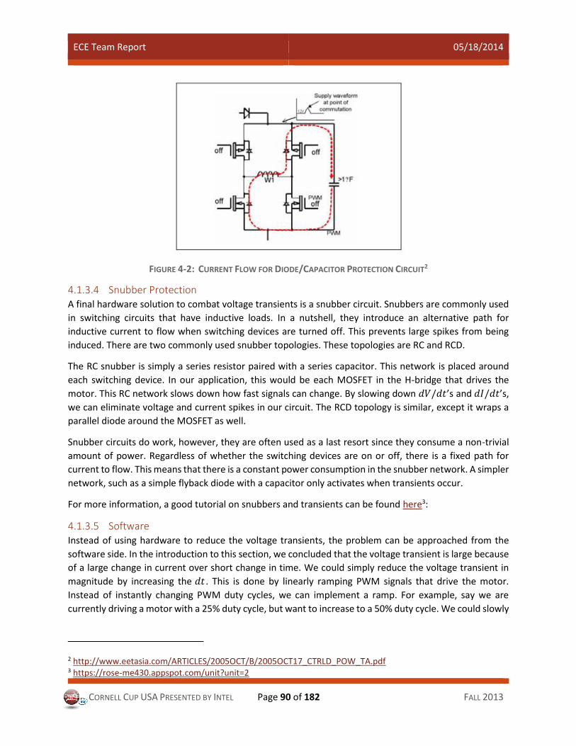
ECE Team Report 05/18/2014
CORNELL CUP USA PRESENTED BY INTEL Page 90 of 182 FALL 2013
FIGURE 4-2: CURRENT FLOW FOR DIODE/CAPACITOR PROTECTION CIRCUIT2
4.1.3.4 Snubber Protection A final hardware solution to combat voltage transients is a snubber circuit. Snubbers are commonly used
in switching circuits that have inductive loads. In a nutshell, they introduce an alternative path for
inductive current to flow when switching devices are turned off. This prevents large spikes from being
induced. There are two commonly used snubber topologies. These topologies are RC and RCD.
The RC snubber is simply a series resistor paired with a series capacitor. This network is placed around
each switching device. In our application, this would be each MOSFET in the H-bridge that drives the
motor. This RC network slows down how fast signals can change. By slowing down 𝑑𝑉/𝑑𝑡’s and 𝑑𝐼/𝑑𝑡’s,
we can eliminate voltage and current spikes in our circuit. The RCD topology is similar, except it wraps a
parallel diode around the MOSFET as well.
Snubber circuits do work, however, they are often used as a last resort since they consume a non-trivial
amount of power. Regardless of whether the switching devices are on or off, there is a fixed path for
current to flow. This means that there is a constant power consumption in the snubber network. A simpler
network, such as a simple flyback diode with a capacitor only activates when transients occur.
For more information, a good tutorial on snubbers and transients can be found here3:
4.1.3.5 Software Instead of using hardware to reduce the voltage transients, the problem can be approached from the
software side. In the introduction to this section, we concluded that the voltage transient is large because
of a large change in current over short change in time. We could simply reduce the voltage transient in
magnitude by increasing the 𝑑𝑡 . This is done by linearly ramping PWM signals that drive the motor.
Instead of instantly changing PWM duty cycles, we can implement a ramp. For example, say we are
currently driving a motor with a 25% duty cycle, but want to increase to a 50% duty cycle. We could slowly
2 http://www.eetasia.com/ARTICLES/2005OCT/B/2005OCT17_CTRLD_POW_TA.pdf 3 https://rose-me430.appspot.com/unit?unit=2

ECE Team Report 05/18/2014
CORNELL CUP USA PRESENTED BY INTEL Page 91 of 182 FALL 2013
ramp towards that 50% duty cycle instead of instantly commanding the PWM to change to 50%. This will
increase the 𝑑𝑡, therefore decreasing the magnitude of the voltage spike.
The benefit of a software solution is that it is versatile and does not add on any cost to the system. Once
hardware is soldered together, it is permanent, or at least more difficult to change. The disadvantage for
our application is that we are trying to use FPGA’s as often as possible. Implementing the control with an
FPGA might be more difficult than simple C code running on an Arduino. Another problem is that a
software solution is not permanent. In the future, for example, someone may comment out the code if
they do not understand what its purpose is. Also, motor deadzones may limit the effectiveness of a
software solution.
Power Board The power board is the main interface between the power source and the powered electronic devices.
Here, it will receive power from the 24 V battery and then regulate that power down to different voltages
levels which are 5 V, 12 V, and also have the option of 24 V (unregulated battery voltage). In addition to
providing different voltages to power a number of components, it also protects these components and
the whole system from overloading or any other unwanted power conditions that could occur
unintentionally. Situations where this could occur are over or under current, voltage, and reverse polarity,
and reverse voltage and current, along with transient voltage and current spikes and noise. A well-
designed power system will lead to optimal scenarios where there will be high efficiency.
4.2.1 Power Board Population As introduced, the power board is the main interface between the power source and the powered
electronic devices. Hence it is crucial for both soldering and multiple checking. Basically, power board
receives the voltage of 24 Volts and transform into the output of 2 different voltages, 0-5 Volts and 0-12
Volts respectively. Additionally, the protection of power board components from overloading or any other
unwanted power conditions are also needed. It may be time-consuming, but from the efficiency
perspective, it is highly recommended to place emphasis on the power board. It will benefit the whole
system in further process.
4.2.1.1 Power Board Schematics The schematics of the power board are shown below:

ECE Team Report 05/18/2014
CORNELL CUP USA PRESENTED BY INTEL Page 92 of 182 FALL 2013
FIGURE 4-3: PCB LAYOUT
FIGURE 4-4: PCB DESIGN
Figure 4-3 shows all the basic components needed and to populate the board. Refer to the components
list for more information. Figure 4-4 shows the full layout and connections between different components.
4.2.1.2 Component list The component list is shown in the figure below:

ECE Team Report 05/18/2014
CORNELL CUP USA PRESENTED BY INTEL Page 93 of 182 FALL 2013
TABLE 4-1: COMPONENTS LIST
4.2.2 Testing One of the major goals after populating the boards this semester was to test the power board to ensure
that it was safely distributing power and the much needed voltages and/or currents. These tests are
imperative to avoid any potential dangers in our circuit such as overcurrent, overvoltage, undervoltage,
spikes in noise or power, reverse voltage, and reverse polarity.
The equipment needed in order to do this testing in addition to the populated power board were the
digital multi-meter (Tektronix DMM 4020 also known as DMM), a power supply (Tektronix PWS 4602),
and alligator clips.
4.2.2.1 Verifying Voltage One of the first things to do for the populated board is to ensure that the correct voltage is coming out.
Initial steps taken to verify the electronic output (5 V and 12 V) were first to turn the power supply on and
set the power supply to 24V to imitate the battery’s voltage and the current limit to 100 mA. Connect the
alligator clips from Vcc and Gnd on the power supply. Once the power supply is set up, now the power
board should be connected in the following order:
1. Connect the power input and output to the battery terminal on the board. Be sure to match the
polarities. This will power the board.
2. Monitor the current delivered by the power supply and verify that the full 100 mA is not being
reached. If it is, immediately stop testing.

ECE Team Report 05/18/2014
CORNELL CUP USA PRESENTED BY INTEL Page 94 of 182 FALL 2013
3. Using the digital multi-meter, measure the 5 V and 12 V bus to ensure that the right voltages are
appearing at these terminals. If the readings are negative of the expected such as -5 V or -12 V, check
the polarities. If the problem still persists, check the components.
4. In addition to verifying that the voltmeter is reading the correct voltage, confirm that the green LEDs
for the 5 V and 12 V are also lit up.
5. Turn off the power supply and disconnect the power board. This ends the electronic output
verification test.
Another test to follow is to verify the motor output with unloaded testing. Initial set up should repeat the
power supply at 24 V set up where the current is still limited to 100 mA. To verify the motor output this
means taking the motor output at 24 V and confirming that nothing is connected to the board externally
at the beginning. Short the two terminals on the breaker block labeled “24 V Breaker” on the board and
before connecting the supply to the board, confirm that the power supply is still set at 24 V. If not, reset
these by turning the knobs on the power supply. Once this is complete, connect the alligator clips from
the Vcc and Gnd for the power supply to the board’s battery.
1. Turn power supply on and look at the board to be aware of any smoking or overheating of
components. If there is, immediately turn the power supply off. The board may be hot if that occurs
so be sure to first turn the power supply off to cut off its power source.
2. Make sure the first LED to light up is the blue LED and only the blue LED at this time.
3. Re-measure the 24 V line to confirm that the line is at 24 V by measuring it with the DMM.
4. Turn the power supply off. Look at the board and notice that the blue LED is still lit up and is again the
only LED that is lit up. This is not an error as the capacitor is discharging. Gradually over a few minutes,
the LED’s light diminishes. Over time the LED will no longer be lit up as the capacitor becomes fully
discharged.
5. Disconnect from the power supply.
A final test to do now is to test the power board and do what is nicknamed a “backwards test.” This
essentially reverses connections and polarities to see if isolation occurs. As per usual, the initial set up
includes the power supply being set at 24 V. Reconfirm that the power supply is at 24 V, once this is done,
do not prematurely connect the alligator clips as this set up will be different from previous tests.
1. Reverse the connections so that the positive voltage is connected to the negative. This test will
determine the safety of the board and power isolation.
2. Monitor the current on the DMM to ensure there is no output. If there is, disconnect the power from
the board immediately. If there is no output, the board is functioning as anticipated.
3. Additionally, verify that the board has no output when the polarities are reversed due to the diode.
The voltage testing on this power board is now complete. These tests ensure that there is no under-
voltage, over-voltage, and reverse polarity.

ECE Team Report 05/18/2014
CORNELL CUP USA PRESENTED BY INTEL Page 95 of 182 FALL 2013
Power Monitoring With any embedded system it is important to know the state of regulated and unregulated currents, and
the present voltage of your battery. This data allows you to know whether something is potentially wrong
with your power board or one of your peripheral attachments, and it provides insight to the state of your
motors so you can safely cut the power supply if they are drawing too much current. There are many
other potential applications of power monitoring as well, so we highly recommend implementing this in
your embedded system!
A few things to consider before starting
1. Before using a microcontroller like an Arduino to analyze power data, it is important to scale voltage
values to a range of between 0V and 5V to avoid destroying your microcontroller. This involves voltage
division with chosen resistances.
2. Think about an appropriate way to display data. It might be useful to display discharge rate or an
estimate of the time remaining in your battery’s charge, for example. We found that displaying the
battery level as a percentage was most advantageous for our purposes.
Items Needed
Measured Load Analysis Data (Voltage vs. Time) - Make sure to connect a load in series with the
battery to draw a constant current.
If you have a Tektronix Digital Multimeter, Labview by Tektronix is great software for this
application.
Graphing software --we suggest:
o LoggerPro Graphing Software (or Graphical Analysis if you have a Mac)
o Excel
o Matlab
The following tutorial involves the use of Logger Pro:
1. Graph the measured data. Graph the measured battery voltage vs. elapsed time from the load analysis on the battery (the data can easily be copied and pasted from an excel spreadsheet). This is your measured battery curve.
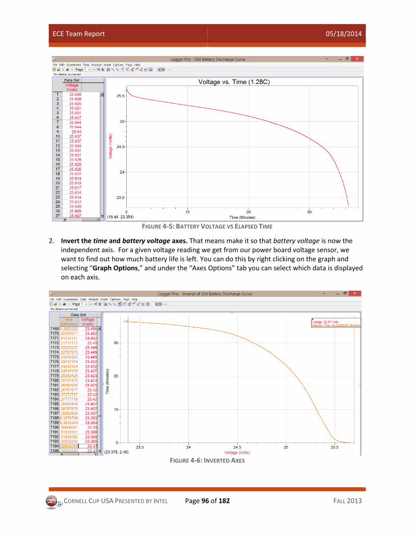
ECE Team Report 05/18/2014
CORNELL CUP USA PRESENTED BY INTEL Page 96 of 182 FALL 2013
FIGURE 4-5: BATTERY VOLTAGE VS ELAPSED TIME
2. Invert the time and battery voltage axes. That means make it so that battery voltage is now the independent axis. For a given voltage reading we get from our power board voltage sensor, we want to find out how much battery life is left. You can do this by right clicking on the graph and selecting “Graph Options,” and under the “Axes Options” tab you can select which data is displayed on each axis.
FIGURE 4-6: INVERTED AXES

ECE Team Report 05/18/2014
CORNELL CUP USA PRESENTED BY INTEL Page 97 of 182 FALL 2013
3. Calculate and graph the battery percentage data. Using the elapsed time data, create a new data set battery percentage, which is the percentage of the battery’s time left. The formula is shown below. Graph these values on the dependent axis instead of the elapsed time data.
% =𝑚𝑎𝑥 𝑒𝑙𝑎𝑝𝑠𝑒𝑑 𝑡𝑖𝑚𝑒 − 𝑒𝑙𝑎𝑝𝑠𝑒𝑑 𝑡𝑖𝑚𝑒
𝑚𝑎𝑥 𝑒𝑙𝑎𝑝𝑠𝑒𝑑 𝑡𝑖𝑚𝑒
FIGURE 4-7: CALCULATE BATTERY PERCENTAGE DATA
FIGURE 4-8: GRAPH BATTERY PERCENTAGE DATA

ECE Team Report 05/18/2014
CORNELL CUP USA PRESENTED BY INTEL Page 98 of 182 FALL 2013
4. Find a relationship that best fits the majority of the data. DO NOT use the Curve Fit option in Logger Pro, it fudges the data and gives values with significant error to allow for a good looking fit to be graphed. For the part of the data beyond the initial battery discharge (less than about 90% battery life), we found that an equation of the following form fit our data well:
In this equation, V is input voltage, is the low battery voltage (where the model curves up into its linear
region), and a affects the slope of the linear part of the model. Constants will need to be calibrated to
best fit the data. For example, we use a 24V battery, and we found that 𝜆 = 23 and 𝑎 = 1.339 fit our
data very well. We suggest using a for() loop in Matlab to iterate through different constants in
your models to more quickly find an equation that fits your data.
6. Find a relationship that best fits the rest of the data. For the initial discharge (battery percentage greater than 90% or so), you may find a linear fit to work better, as this part of the battery discharge does not follow the trend that the rest of that data does, so the model suggested previously will not fit it. You may also want your battery to read as full if you are above this threshold. We also found that our model diverges a little bit towards low percentages (ie < 2%), so it is advisable to set a minimum percent to display (or an automatic shutdown if a critical battery level is reached).
7. You now have a piecewise model of the discharge curve! For a given voltage value, you can now predict the battery percentage. This can be easily implemented using a microcontroller with a voltage sensor.
4.3.1 Notes on Current and Voltage Sensing The current and voltage sensors necessary for power monitoring are part of the power board itself. The
current sensor is a high-side current sensing resistor based op-amp amplifier - the resistor is used as the
current to voltage conversion element whereas the op-amp is used to amplify the small voltage to a larger
one that can easily be detected by the microcontroller/Arduino ADC.
While this sounds simple in functionality, it took a while to get the current sensing part working. It seemed
to be working for low currents but giving no output at higher currents. This seemed unreasonable due to
the simplicity of the circuit which did not seem to have any reason to behave like it did, at least on paper.
Initially, we speculated that the problem could have been due to noise on the op-amp output and thus a
low pass filter was placed on the op-amp output. This made the situation better (increased the range over
which the circuit worked) but did not solve it completely since the current sensing was not working
correctly over the entire required current range (it still had the same problem at higher currents).
The solution to this problem was placing decoupling/bypass capacitors on the op-amp power supply lines.
The 5V supply that was supplying the power to the op-amps seemed to be noisy and this hampered the
op-amp's operation, especially at higher op-amp input voltages (higher currents through the resistor).
Placing two 0.1𝜇𝐹 capacitors near the op-amp supply lines (one for each of the sensing op-amps), along
with a 15𝜇𝐹 capacitor (all in parallel across the 5V line) seemed to fix the noise issue. The low-pass filter
at the op-amp output was not required and was then thus removed. The current sensing part worked as
desired just with the additional capacitors on the power lines.

ECE Team Report 05/18/2014
CORNELL CUP USA PRESENTED BY INTEL Page 99 of 182 FALL 2013
The changes to the circuit (addition of capacitors) were done on the already populated PCBs as the
addition could be simply done by scraping the soldermask off and soldering the capacitors on the top side
of the board instead of having to redesign and repopulate the entire PCB.
New Battery Selection The current battery packs that are used in our ModBot and most recent iteration, the Dunebot, contain
eight 3.2 volt cells configured in series resulting in a total of 25.6 volts. The capacity of the pack is 2500mAh
which came as a standard specification of the LiFePO4 cell we chose. However, R2-I2 has higher power
demands.
4.4.1 The New Battery Two tentative options are possible:
(1) One option is to simply put two battery backs in parallel. However, due to cell balancing, complexities
arise with such a situation.
(2) The other option is to order a new battery pack with twice the number of cells and having pairs of
cells in parallel. In addition, we’d be using new larger capacity cells.
4.4.2 The New Cell Along with our search for a new battery, we found a new LiFePO4 cell with a larger capacity being sold by
the supplier. It was the same size and voltage rating but had a capacity of 3300mAh. Therefore we’d get
more capacity without sacrificing space. However, the maximum continuous current it supported was
9.9A. Much less than what we need for R2-I2. Then in the case of using this cell for the battery pack,
doubling the number of cells is necessary anyways so as to double the supported continuous current.
4.4.2.1 New Cell Load Analysis To confirm that the new cell would live up to its specifications, we tested the cell. We loaded the cell with
a 1.1Ω high-power resistor, discharging the cell at 2.9A. We estimated that it would last approximately 70
minutes using the following formula:
𝑅𝑢𝑛 𝑇𝑖𝑚𝑒 (𝑚𝑖𝑛𝑢𝑡𝑒𝑠) =𝑏𝑎𝑡𝑡𝑒𝑟𝑦 𝑐𝑎𝑝𝑎𝑐𝑖𝑡𝑦 (𝐴ℎ)
𝑎𝑣𝑒𝑟𝑎𝑔𝑒 𝑐𝑢𝑟𝑟𝑒𝑛𝑡 𝑑𝑟𝑎𝑤 (𝐴𝑚𝑝𝑠)×
60 𝑚𝑖𝑛𝑢𝑡𝑒𝑠
1 ℎ𝑜𝑢𝑟
The results of the load analysis confirmed the capacity of the cell and can be found in the figure below.
Refer to section 4.4.3 for more details on the procedure.

ECE Team Report 05/18/2014
CORNELL CUP USA PRESENTED BY INTEL Page 100 of 182 FALL 2013
FIGURE 4-9: BATTERY DISCHARGE CURVE
4.4.3 Battery Testing Procedure This can also be found in prior documentation done by Mike. The only difference is one additional
subsection.
4.4.3.1 Using a Computer with Tektronix DMM 4020 Before we can record voltages at multiple time intervals using our digital multimeter we need to ensure
the appropriate software is installed correctly.
What You Need:
NI LabVIEW SignalExpress Tektronix Edition installation CD
LabVIEW SignalExpress Step for DMM4020 v1.0 Download (Creation of account necessary).
Tektronix DMM 4020 Digital Multimeter
R232 Serial Cable
The Process:
1. Insert NI LabVIEW SignalExpress Tektronix Edition Installation CD into your computer and begin the
installation. When it asks you whether you would like to install the Tektronix Edition or the LE version,
choose the LE version, unless you have the product key for the Tektronix edition. However, the extra
features of the Tektronix edition are not needed for our purposes. Continue the installation as normal.
2. Now we must install the LabVIEW SignalExpress Step for DMM4020 v1.0. If you haven’t already, get
it from the download link in section 0. Once you have the file, run it. Once it’s done installing, you
have the necessary software installed to use your DMM4020 with the computer!
3. Connect your DMM4020 to your computer using an R232 serial cable. If you instead have a USB-to-
R232 cable, that will work as well but you must be sure to have the drivers installed correctly. Go to
0.0
1.0
2.0
3.0
4.0
0 10 20 30 40 50 60 70 80
Vo
ltag
e
Time (min)
LiFePO4 26650 Cell Discharge Curve at 2.9A/.87C
New 3.3Ah Cell 2.75V Cutoff

ECE Team Report 05/18/2014
CORNELL CUP USA PRESENTED BY INTEL Page 101 of 182 FALL 2013
your Device Manager and make note of which Serial COM port your DMM4020 is connected to. You’ll
need that later.
4. Run LabView SignalExpress. You’ll be greeted with a dialogue box asking you what type of project you
want to begin with, choose Start with an Empty Project.
5. At the top of the window go to Add Step → Tektronix → Acquire Signals → Tek DMM4020.
6. A new Step will show up on the window work area. Under Resource Name, choose the COM port
designated to your DMM4020 that you looked up earlier.
7. You’re ready to acquire signals!
I-3P0 Power Supply Because of the low mobility of the I-3P0 robot and its very high power demand, it was quickly decided
that it would be a tethered system utilizing an external AC-DC power supply. Since these types of supplies
are very difficult to design and build, they can be very expensive, and most importantly they can be very
dangerous to work with because of their 120V operating voltage. It is highly recommended that these
power supplies be purchased from a reputable power supply manufacturer. The rest of this section will
explain how to correctly pick out the right power supply, and how we wired up our power supply for I-
3P0.
4.5.1 System Requirements 4.5.1.1 Voltage The very first thing to consider is what voltages the system requires. The most common voltages used are
24V, 12V, 5V, and 3.3V. On I-3P0 there are systems running 24V, 12v, and 5V. However, since the 12V rail
is only used to power the onboard Intel motherboard, our team decided to only implement a 24V rail and
5V rail using external power supplies. These would power the very large motors and all the servos on the
robot. The 12V power rail would be provided by our onboard power board, in order to run the Intel
motherboard and some of the small auxiliary chips. The power board steps down 24V to 5V and 12V for
lower current applications.
4.5.1.2 Current Once we have selected our 2 required voltages (2V4 and 5V), the next step is to determine how much
current each of these rails will require. The amount of current that a power supply can provide is directly
correlated to its cost, size, and power output. For the 5V supply, we were running at least 10 servos, with
an expected current draw of at most 1A each. To give us some overhead, we selected a power supply at
150% of our expected draw, resulting in a 15A desired current.
For the 24V power supply, we were powering much more. First we needed to power our power board and
Intel motherboard, which should draw a max of 1A. Next we had to power several auxiliary motors, which
were rated at roughly 4A each. We expected there to be about 4 of these motors. Finally we had to power
the enormous walking motor and torso motor, which were rated at 40A and 10A respectively. Totaling
this expected power draw sums to about 65A of power. Knowing that this is an extremely high estimation
to be cautious, and also realizing that 65A at 24V is over 1500 watts of power, we did not add any
additional overhead to this estimation and targeted a 65A power supply.

ECE Team Report 05/18/2014
CORNELL CUP USA PRESENTED BY INTEL Page 102 of 182 FALL 2013
4.5.2 Purchasing At this point we researched for the two power supplies desired for this system and settled on Mean Well
as the power supply manufacturer of our choice. They build excellent power supplies which have many
safety features built in. Look for power supplies with thermal and overcurrent protection, as well as
current limiting and remote on/off features. The HRP-75-5 satisfied our requirements for a 5V supply, and
the RSP-1500-24 satisfied our requirements for the 24V supply. We would recommend purchasing from
www.trcelectronics.com as a reputable power supply distributer.
FIGURE 4-10: HRP-75-5 POWER SUPPLY FIGURE 4-11: RSP-1500-24 POWER SUPPLY
4.5.3 Installation 4.5.3.1 External Case If you purchase an “enclosed type” power supplies like the ones we selected above, the connections
completely exposed on the front. These power supplies need to be housed in a very safe case. TRC
Electronics provides two different power supply cases that will fit almost all standard power supplies sold
on their website. Any case that you use must allow you to very securely mount the power supply inside,
it must be completely insulated OR properly grounded if it’s metal, it must provide proper ventilation and
cooling, and it should securely close fully to prevent anything or anyone from accidently coming in contact
with the live connectors. Because our system required an enormous 1500W power supply, we were
unable to purchase a standard power supply case and needed to fabricate one ourselves to meet all the
above requirements.
FIGURE 4-12: CUSTOM POWER SUPPLY CASE

ECE Team Report 05/18/2014
CORNELL CUP USA PRESENTED BY INTEL Page 103 of 182 FALL 2013
We built a large acrylic case to hold the power supplies, and made all the walls out of plastic or clear acrylic
to ensure that the case was non-conducting. There are two fans opposite each other on the two furthest
walls, both blowing in the same direction to keep air flowing through the case. This in important to keep
the power supplies cool. Finally, the top of the case was where we mounted all the master switches,
lockouts, indicator lights, and circuit breakers. The two sides of the case had holes cut in them to allow
the final output wires and input power plug to stick out of the case safely. A voltage danger sticker was
also applied to the case to warn others of the potential shock hazard.
4.5.3.2 Wire Gauge For all the power supply wiring, it is extremely important to use the correct gauge wire for the expected
currents. Undersized wire can add resistance, heat up, and even melt or start fires. We used 18 gauge
wire or higher for the high voltage 120V lines, 12 gauge wire or higher for all the low voltage 5V outputs,
and DOUBLE runs of 12 gauge wire for the 24 volt output because of its extremely high current capability.
It is always better to use a thicker wire when possible, especially when using long runs of transmission
cables like we are to connect I-3P0 to the power supplies. Even though both power supplies together are
capable of about 1600 watts and over 60 amps on the outputs, there is only a maximum of 1600W/120V
= 13.3A of current running through the high voltage 120V wires, which is why they can be run with smaller
wire.
FIGURE 4-13: WIRE GAUGE CURRENT LIMITS

ECE Team Report 05/18/2014
CORNELL CUP USA PRESENTED BY INTEL Page 104 of 182 FALL 2013
4.5.3.3 Wiring Schematic
FIGURE 4-14: WIRING SCHEMATIC
Both power supplies were directly connected to the Neutral and Ground wires of the external AC power
plug. However, the Hot wire was first connected to a 12A thermal circuit breaker which will limit the
overall power draw from the wall outlet to 1440A. Most home electrical outlets will trip their circuit
breakers at 1800 watts, which ensures that this power supply will not trip a home electrical circuit breaker
by itself. Be sure to check which wire is the Hot wire by looking at the diagram of a standard North
American power outlet below.
FIGURE 4-15: NORTH AMERICAN 120V OUTLET
After the circuit breaker, the Hot 120V line divides between 2 main power switches, which stick out of the
top of the power supply. These switches are on the high voltage side so they cannot withstand higher the
15A of current, and this design also allows them to completely remove power from the power supplies
themselves, not just the robot. Next, each switch is wired into the Hot input of the power supplies, and
the power supply outputs are each wired to an indicator LED and an extremely large electrolytic capacitor
(100,000𝜇𝐹) to help prevent large power demand spikes from disrupting the AC power supplies. Because
AC power supplies operate primarily through a transformer, they are very poor at working under rapid
current changes. They cannot change their current output rapidly like a battery or a capacitor can, so
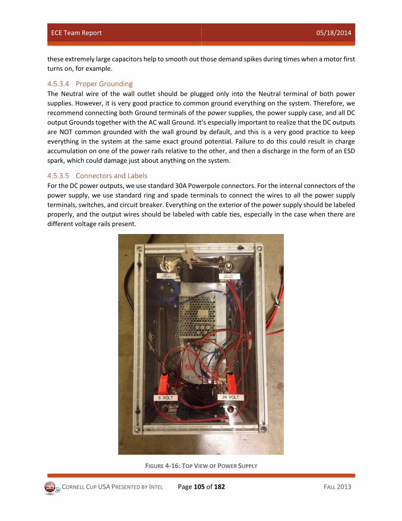
ECE Team Report 05/18/2014
CORNELL CUP USA PRESENTED BY INTEL Page 105 of 182 FALL 2013
these extremely large capacitors help to smooth out those demand spikes during times when a motor first
turns on, for example.
4.5.3.4 Proper Grounding The Neutral wire of the wall outlet should be plugged only into the Neutral terminal of both power
supplies. However, it is very good practice to common ground everything on the system. Therefore, we
recommend connecting both Ground terminals of the power supplies, the power supply case, and all DC
output Grounds together with the AC wall Ground. It’s especially important to realize that the DC outputs
are NOT common grounded with the wall ground by default, and this is a very good practice to keep
everything in the system at the same exact ground potential. Failure to do this could result in charge
accumulation on one of the power rails relative to the other, and then a discharge in the form of an ESD
spark, which could damage just about anything on the system.
4.5.3.5 Connectors and Labels For the DC power outputs, we use standard 30A Powerpole connectors. For the internal connectors of the
power supply, we use standard ring and spade terminals to connect the wires to all the power supply
terminals, switches, and circuit breaker. Everything on the exterior of the power supply should be labeled
properly, and the output wires should be labeled with cable ties, especially in the case when there are
different voltage rails present.
FIGURE 4-16: TOP VIEW OF POWER SUPPLY

ECE Team Report 05/18/2014
CORNELL CUP USA PRESENTED BY INTEL Page 106 of 182 FALL 2013
4.5.3.6 24V Key Lockout A special feature of this power supply is the 24V key lockout switch. This is feature is made possible by
the remote on/off and 12V auxiliary output of the large 24V power supply. Using a standard electronic
key switch, we followed the datasheet for the power supply to enable a remote on/off, and setup the key
switch so that when the key was turned, the switch was closed and the power supply turned on. If the key
is removed, the switch is opened and the power supply will turn off, even when external AC power is still
supplied. This is a great safety feature for the 1500W power supply to ensure only authorized operators
can turn on the power supply, even when it is plugged in and the smaller 5V supply is on.
FIGURE 4-17: REMOTE ON/OFF WIRING DIAGRAM
5 Microcontroller Selection Galileo
5.1.1 Getting Started + Setting Up Galileo WiFi Before using the Galileo at all, you must make sure the system is up to date. Intel has conveniently
provided a Getting Started Document at https://communities.intel.com/docs/DOC-21838 which is where
you should go first. Within the document, it will tell you what to do enable WiFi on the Galileo if you wish
to. When asked for, extra software can be found here: https://communities.intel.com/docs/DOC-22226.
For WiFi: Once the Galileo is prepped, finding a supported WiFi card and confirming the correct drivers
are installed is next. A guide to do that is at http://www.malinov.com/Home/sergey-s-blog/intelgalileo-
addingwifi.
5.1.2 Arduino One of the hallmarks of the Galileo is that it can be programmed with Arduino. As of now, it only requires
a custom Arduino IDE provided at Intel’s website and can be found at
https://communities.intel.com/docs/DOC-22226 for your respective OS. Be warned that some important
functions found in the Arduino library are not yet supported. These are documented and can be found in
the Galileo Release Notes at https://communities.intel.com/docs/DOC-21837.

ECE Team Report 05/18/2014
CORNELL CUP USA PRESENTED BY INTEL Page 107 of 182 FALL 2013
5.1.3 C/C++ It is possible to write and compile raw C++ code for the Galileo. While it is true that Arduino code is actually
C code, sometimes you want more flexibility than the Arduino environment allows.
The Galileo itself does not come with a C++ compiler. Therefore, code needs to be compiled on a separate
computer, then the executable transferred over to the Galileo. The Galileo requires a specialized compiler,
which happens to come with the Arduino software at https://communities.intel.com/docs/DOC-22226.
To run this specialized compiler, use the Makefile at https://github.com/tokoro10g/galileo-makefile,
following the provided directions. If you are still unable to compile after following the directions, it may
be necessary to execute the following commands:
$ cd /where/you/extracted/the/archive/arduino-1.5.3
$ cd hardware/tools/sysroots
$ sudo mkdir -p /opt/clanton-tiny/1.4.2
$ sudo mv . /opt/clanton-tiny/1.4.2
On Ubuntu Linux 12.04, this solved an issue where the system couldn’t find the libraries necessary to run
the Galileo C++ compiler.
5.1.4 Moving files to the Galileo Say you have a file on your local machine, “/path/to/file.txt”, and you would like to move this to the
Galileo. The simplest way to do this is using the Linux SCP utility. If you’re using windows, it can also be
acquired using Cygwin (with the “openssh” package): http://www.cygwin.com/.
The syntax for SCP is:
$ scp /path/to/file.txt [email protected]:/where/to/copy
where “192.168.1.114” is the IP of the Galileo, and “/where/to/copy” is the directory you’d like to copy
the file to.
5.1.5 Programming GPIO from Linux It is possible to control pins on the Galileo board using linux filesystem I/O. This is useful because it allows
all programming languages with file I/O capabilities to do GPIO. The interface is described at
http://www.malinov.com/Home/sergey-s-blog/intelgalileo-programminggpiofromlinux. For an example,
see the Python section below.
5.1.6 Python Python is built into the default Galileo OS. Using the linux GPIO interface, Python is able to do I/O through
the GPIO pins. The following program blinks the built-in LED every second for 10 seconds.
import os, time
os.system("echo -n '1' > /sys/class/gpio/gpio55/value")
os.system("echo -n 'out' > /sys/class/gpio/gpio39/direction")
echo -n "strong" > /sys/class/gpio/gpio27/drive

ECE Team Report 05/18/2014
CORNELL CUP USA PRESENTED BY INTEL Page 108 of 182 FALL 2013
for i in range(10): os.system("echo -n '%d' > /sys/class/gpio/gpio39/value" % (i % 2))
time.sleep(1)
For more information on the system commands, see the above “Programming GPIO from Linux” section.
5.1.7 Main Issues with Galileo Board We were originally planning on putting both the power monitoring system and the IMU on the Galileo
board, but after trying out the Galileo board, we ran into unresolvable issues and thus had to go back to
the Arduino board we were used to using.
One problem was that not all functions and libraries are supported on the Galileo, e.g. the pulseIn function
used to read pulse widths of input PWM signals was not available. Another problem was that the Galileo
could only run Arduino code at around 74 Hz because it was using Linux to simulate an Arduino. This is
much slower than an Arduino’s computing rate of 700 kHz, and can only be fixed by writing C code for the
Galileo instead of Arduino code. Unfortunately, this means we would have to write in low level C
code. And a final inconvenience is that there is no internal memory on the Galileo, which means we need
a microSD card to upload code.
There were some specific problems with using the Galileo board for power monitoring too. For one thing,
we could not use the external voltage reference (AREF) on the board for the analog-to-digital conversion
(ADC), so if our main power voltage drifted, all of our values would be inaccurate. Additionally, to use the
Galileo’s internal ADC, our system must pass signals through a port expander, which has a 2ms latency
that lags the system and also creates a slight voltage drop before the actual output pin, further removing
accuracy of our system. Practically, the Galileo’s ADC has a much lower impedance tolerance than the
Arduino’s ADC so if the voltage readings from the power board was not buffered correctly, we would get
more bad readings. Finally, physical touching of components near the circuit on the Galileo board caused
the Linux kernel to crash, forcing us to manually reset the board or even re-upload code to continue
operations. All in all, the Arduino board had less disadvantages than the Galileo board, so we went with
it.
6 Motor Control We want very precise digital control so we ignore analog, RC and open loop commands. We use simple
serial commands to ensure that our high level systems handle all the intelligent calculations, so motor
controller just controls. We recommend using Sabertooth 2 X12 and 2 X 25, because we had jittering
problems with the Syren 25.
Sabertooth 2x25 Motor Controller 6.1.1 Introduction The Sabertooth 2x25 motor fits our application well. It has a wide range of acceptable inputs, spanning
from 6V up to 30V. It also has plenty of output current to drive the motors that the mechanical engineering
team selected. The Sabertooth can source up to 25A of continuous current from each channel, and can
temporarily source up to 50A per channel for a few seconds. An additional important feature is that

ECE Team Report 05/18/2014
CORNELL CUP USA PRESENTED BY INTEL Page 109 of 182 FALL 2013
Sabertooth has overcurrent and thermal protection, which will be invaluable in enforcing safety and
circuit reliability.
FIGURE 6-1: SABERTOOTH 2X25 MOTOR CONTROLLER
The purpose of this section is to inform the reader on how to setup and operate the Sabertooth 2x25 in
either analog or serial modes.
6.1.2 Materials Sabertooth 2x25 Motor Controller
Desktop PC running Windows 7
Tektronix PWS4602 Programmable DC Power Supply
2x Anaheim Automation DC Motors BDS-28-38-24
USB to TTL Converter Cable
2x Potentiometers
6.1.3 Controlling the Sabertooth 2x25 As previously mentioned, the Sabertooth has a variety of modes of operation. These include analog, radio,
serial, and packetized serial. In R2-I2 the mode used was simple serial. Before connecting the controller
to a computer to send it serial commands, however, the analog mode is be used to verify the controller.
6.1.3.1 Analog Mode Analog mode allows us to independently control the speed and direction of two DC motors with a voltage
between 0V to 5V. The following steps set us up for operation in this mode.
1. Setting the Switch Panel. The Sabertooth has a total of six switches that can either be in the up or
down position. For analog mode, we want the switch positions to be as follows:

ECE Team Report 05/18/2014
CORNELL CUP USA PRESENTED BY INTEL Page 110 of 182 FALL 2013
FIGURE 6-2: SWITCH POSITIONS FOR ANALOG MODE
This sets the motor controller for lithium, analog input, independent motor control, and linear control.
2. Connecting the B Leads. With the switch panel correctly configured, the next step is to start making
connections to the motor controller. With the power supply off, connect the negative lead of the
power supply to the B- port of the motor controller. Next, connect the positive lead of the power
supply to the motor controller B+ port.
3. Connecting the First DC Motor. With the power connections made to the motor controller, we can
now attach the two DC motors. There will be two leads coming off of the motor. Connect one of them
to the M1A port of the motor controller and connect the other to the M1B port. The order is arbitrary
for the purposes of this setup. Connecting the leads in an opposite orientation will simply make the
motor spin in the other direction.
4. Connecting the Second DC Motor. Repeat the steps above, but this time attach the second DC motor
to the M2A and M2B ports of the motor controller.
5. Connecting the Potentiometers. Now that we have made the connections to the DC motors, the final
step is to setup the signal lines. On the other side of the motor controller, there are green screw-
terminals. The potentiometers will have three outputs. There should be a red, a black, and a yellow
wire coming off of the potentiometer. If this is not true, then please solder a red jumper wire to pin 1
of the potentiometers, a yellow wire to pin two of the potentiometers, and a black wire to pin 3 of
the potentiometers. Screw in the red jumper wire of both potentiometers into the port labeled “5V.”
Next, screw in the black jumper wires into the port labeled “0V.” Connect the yellow wire of the first
potentiometer into the S1 port, and finally, connect the yellow wire of the second potentiometer into
the S2 port.
6. Turning On Power. Now the system is ready to go. You may turn on the power supply, but do not turn
on the output just yet. First set the voltage output to about 12VDC. Limit the current to about 1.5A.
Before turning on the output, verify that the wiring is correct. You may want to make sure that both
potentiometers are set to approximately the middle before turning the output on, that way both
motors are off, or spin slowly. You may now turn on the output.
7. Controlling the Motors with Analog Voltages. In analog mode, a signal from 0V to 5V on the S1 and
S2 ports independently controls motor 1 and 2, respectively. A 0V signal will tell the motor to go in
full reverse. A 5V signal, will similarly tell the motor to go full forward. A 2.5V signal will halt the motor.
As you may have guessed, sweeping the signal from 2.5V to 5V will linearly increase the speed of the
motor in the forward direction. Sweeping from 2.5V down to 0V will similarly increase the speed in

ECE Team Report 05/18/2014
CORNELL CUP USA PRESENTED BY INTEL Page 111 of 182 FALL 2013
the reverse direction. You should now have full control over both DC motors with the two
potentiometers. Have Fun!
6.1.3.2 Simple Serial Mode Simple serial mode allows us to independently control the speed and direction of two DC motors with an
8-bit packet. These 8-bits can be sent from a microcontroller, or PC.
1. Setting the Switch Panel. The Sabertooth has a total of six switches that can either be in the up or
down position. For simple serial mode, we want the switch positions to be as follows:
FIGURE 6-3: SWITCH POSITIONS FOR SIMPLE SERIAL MODE
This sets the motor up for simple serial mode. A one byte packet is sent to control a motor. If you have
already wired and set up the motor controller for analog mode, you may skip to step 5.
2. Connecting the B Leads. With the switch panel correctly configured, the next step is to start making
connections to the motor controller. With the power supply off, connect the negative lead of the
power supply to the B- port of the motor controller. Next, connect the positive lead of the power
supply to the motor controller B+ port.
3. Connecting the First DC Motor. With the power connections made to the motor controller, we can
now attach the two DC motors. There will be two leads coming off of the motor. Connect one of them
to the M1A port of the motor controller and connect the other to the M1B port. The order is arbitrary
for the purposes of this setup. Connecting the leads in an opposite orientation will simply make the
motor spin in the other direction.
4. Connecting the Second DC Motor. Repeat the step above, but this time attach the second DC motor
to the M2A and M2B ports of the motor controller.
5. Connecting to the PC. Now that we have made the necessary power connections to the motors and
DC power supply, we can make the signal connections. Using the USB to TTL converter cable, connect
the TXD pin to the S1 port of the motor controller you also need to connect the RXD pin to the S2 port
of the motor controller. The TXD pin is the orange cable on the USB while the RXD pin is the yellow

ECE Team Report 05/18/2014
CORNELL CUP USA PRESENTED BY INTEL Page 112 of 182 FALL 2013
cable on the USB. You also need to connect the 0V pin of the Sabertooth to ground of the USB to TTL
converter cable, which in this case is the black pin of the cable.
FIGURE 6-4: PINOUT FOR USB TO TTL CONVERTER CABLE
6. Downloading the Pololu Serial Transmitter Utility. If the Pololu Serial Transmitter Utility hasn’t been
installed on your computer yet, please install it from this link: http://www.pololu.com/docs/0J23.
Once installed, please open the program. You should see the following window:
FIGURE 6-5: POLOLU SERIAL TRANSMITTER UTILITY INTERFACE
7. Setting Up the Pololu Serial Transmitter Utility. Under the COM Port listbox, select the COM port
that the Sabertooth is connected to. If you do not know what COM port the motor controller is
connected to, then press the windows key and type “device manager.” Press the enter key. On the
menu that pops up, scroll down to “Ports (COM and LPT).” Locate the device listed as USB Serial Port,
then locate the COM port next to it. Verify that the Baud Rate textbox is set to “9600 bps.”
8. Turning On Power. Now the system is ready to go. You may turn on the power supply, but do not turn
on the output just yet. First set the voltage output to about 12VDC. Limit the current to about 1.5A.

ECE Team Report 05/18/2014
CORNELL CUP USA PRESENTED BY INTEL Page 113 of 182 FALL 2013
Before turning on the output, verify that the wiring is correct. You may now turn on the output. One
blue LED should now be continuously on.
9. Controlling the Motors with Serial Commands. We are now ready to send commands from the Pololu
Serial Transmitter. To enter a command, place text in the single byte box, then press the “send single
byte” button. The commands are:
[0]: Command motors 1 and 2 to stop
[1]: Command motor 1 to go full reverse
[64]: Command motor 1 to stop
[127]: Command motor 1 to full forward
[128]: Command motor 2 to go full reverse
[192]: Command motor 2 to stop
[255]: Command motor 2 to go full forward
Notes:
You may enter commands in decimal form, or hexadecimal with a 0x in front.
If you do not want the motor to spin at full speed (forward or reverse), you may enter a value in
between. For example. If 1 is full reverse and 64 is stop. Then sending a command of 32 will
make motor 1 spin at approximately half speed.
6.1.4 Kangaroo Motion Controller The Kangaroo is a motion control device that helps record values of motion control and other useful values
such as maximum motor speed, motor limit positions, and PID values after tuning. The other benefit of
using the Sabertooth and Kangaroo is the communication between them with their software, DesCribe.
DesCribe software can be used to program the Kangaroo or Sabertooth to what is required.
In order to use the Kangaroo with the Sabertooth you must connect the Kangaroo to the Sabertooth (See
Section 6.3).
The DIP switches on the Kangaroo have two states which include “on” and “off.” The state of a switch can
be changed by sliding the switch to the opposite state with either a pen or small screwdriver. Please note
that you should only change DIP switches when the Kangaroo is powered off. The figure below
summarizes the Kangaroo DIP switches.

ECE Team Report 05/18/2014
CORNELL CUP USA PRESENTED BY INTEL Page 114 of 182 FALL 2013
FIGURE 6-6: KANGAROO DIP SWITCHES
Switch 1
Switch 1 toggles the Kangaroo between analog input and digital input modes. In most cases, you will most
likely want the Kangaroo set to Digital Input mode. In digital input mode, the Kangaroo accepts TTL serial
commands, which are convenient when using an Arduino or PC. Analog mode allows the Kangaroo to
accept 0-5V analog signals.
Switch 2
Switch 2 toggles the Kangaroo between analog feedback and quadrature feedback modes. In most motor
control situations, you will want Switch 2 on for quadrature feedback mode. When in this mode, the
Kangaroo accepts input from an encoder connected to the Feedback inputs A and B. Analog feedback
relies on physical DC voltage levels for feedback.
Switch 3
Switch 3 toggles the Kangaroo between velocity and position control. The position of this switch is not
critical, as it is overridden when TTL serial commands are sent to the Kangaroo. We had the switch set to
on, since the other three switches are also kept on.
Switch 4
The final switch, Switch 4, toggles the Kangaroo between mixed and independent modes. We found
independent mode to be the more versatile mode in our application, therefore we have the fourth switch
set to “on”. Independent mode allows you to send a motor channel (1 or 2), followed by a command to
the Kangaroo. If using mixed mode, the commands control both channels are the same time. For example,
a D command (drive), spins both wheels in the same direction. A T command (turn), spins one wheel
forward and the other backward. This mode is convenient for tank-style robots, but takes away some
control from the programmer.

ECE Team Report 05/18/2014
CORNELL CUP USA PRESENTED BY INTEL Page 115 of 182 FALL 2013
Note: Changing DIP switches may require you to redo tuning. Switches 1 and 3 can be changed without
having to tune again, but changing switches 2 or 4 will cause the Kangaroo to not operate. In order to get
the Kangaroo working again, you will need to perform tuning again or put switches 2 and 4 back to the
state that they were in when the motor was tuned.
In our design we left all the switches on. This was because we wanted to use simple serial commands to
control the motor controller and run the motors in independent mode.
RoboClaw 2x15 Motor Controller 6.2.1 Introduction The RoboClaw 2x15 motor controller was another candidate that we considered using to drive R2-I2’s
motors. Like the Sabertooth 2x25, the RoboClaw fit our application well. It accepts a wide range of inputs,
spanning from 6V up to 34V. It also has plenty of output current to drive the motors that the mechanical
engineering team selected. The RoboClaw can source up to 15A of continuous current from each channel,
and can temporarily source 30A per channel for a few seconds. Like the Sabertooth, the RoboClaw also
has overcurrent and thermal protection.
FIGURE 6-7: ROBOCLAW 2X15 MOTOR CONTROLLER
The purpose of this section is to inform the reader on how to setup and operate the RoboClaw 2x15 in
either analog or serial modes.
6.2.2 Materials RoboClaw 2x15 Motor Controller
Desktop PC running Windows 7
Tektronix PWS4602 Programmable DC Power Supply
2x Anaheim Automation DC Motors BDS-28-38-24
USB to TTL Converter Cable
2x Potentiometers

ECE Team Report 05/18/2014
CORNELL CUP USA PRESENTED BY INTEL Page 116 of 182 FALL 2013
Female to Female Jumper Wires
6.2.3 Controlling the RoboClaw 2x15 As previously mentioned, the RoboClaw has a variety of modes of operation. These include analog, radio,
serial, and packetized serial. If this motor controller had been the final one selected for R2-I2 the mode
that be used would have been simple serial. Before connecting the controller to a computer to send it
serial commands, however, the analog mode is used to verify the controller.
6.2.3.1 Simple Serial Mode 1. Connecting the + and – Leads. The first step is to start making connections to the motor controller.
With the power supply off, connect the negative lead of the power supply to the (-) port of the
motor controller. Next, connect the positive lead of the power supply to the motor controller (+)
port.
2. Connecting the First DC Motor. With the power connections made to the motor controller, we
can now attach the two DC motors. There will be two leads coming off of the motor. Connect one
of them to the M1A port of the motor controller and connect the other to the M1B port. The
order is arbitrary for the purposes of this setup. Connecting the leads in an opposite orientation
will simply make the motor spin in the other direction.
3. Connecting the Second DC Motor. Repeat the step above, but this time attach the second DC
motor to the M2A and M2B ports of the motor controller.
4. Connecting to the PC. Use a female to female jumper wire to make a connection from the USB
TXD pin to the S1 port of the motor controller. Please note that there are three pins in the S1 row.
The pin closest to the “S1” on the board is the pin that you should make the connection to.
Next use another female to female jumper wire to make a connection from the USB GND pin to
the S1 port of the motor controller. This time, connect to the back pin of the S1 header.
FIGURE 6-8: PINOUT FOR USB TO TTL CONVERTER CABL
5. Downloading the Pololu Serial Transmitter Utility. If the Pololu Serial Transmitter Utility hasn’t
been installed on your computer yet, please install it from this link:
http://www.pololu.com/docs/0J23. Once installed, please open the program. You should see the
following window:

ECE Team Report 05/18/2014
CORNELL CUP USA PRESENTED BY INTEL Page 117 of 182 FALL 2013
FIGURE 6-9: POLOLU SERIAL TRANSMITTER UTILITY INTERFACE
6. Setting Up the Pololu Serial Transmitter Utility. Under the COM Port listbox, select the COM port
that the RoboClaw is connected to. If you do not know what COM port the motor controller is
connected to, then press the windows key and type “device manager.” Press the enter key. On
the menu that pops up, scroll down to “Ports (COM and LPT).” Locate the device listed as USB
Serial Port, then locate the COM port next to it. Verify that the Baud Rate textbox is set to “9600
bps.”
7. Turning On Power. The next step is to turn on the power supply, but do not turn on the output
just yet. First set the voltage output to 12VDC. Limit the current to about 1.5A. Verify that the
wiring is correct, then turn on the output.
Verify that there is a jumper in place across the LB-MB pins. Shorting these pins allows the motor
controller to power its logic from the battery (DC power supply in our experiment), instead of an
external 5V source.
8. Configuring the Roboclaw for Simple Serial Mode. Before we can have fun with motors, we first
need to set the mode on the RoboClaw. On the logic side of the RoboClaw, there are three small
push-buttons labeled “MODE”, “SET,” and “LIPO.”
Hold down the MODE button for approximately one second, then release it. The first LED will blink
a certain number of times. This blinking tells you what mode you are in. For simple serial, we want
the light to blink 5 times. Use the MODE and SET buttons to increase/decrease the blinks, until 5
is reached. Hold down the LIPO button to confirm and save the new setting.
9. Controlling the Motors with Serial Commands. From the Pololu Serial Transmitter, begin sending
single byte commands. The possible commands are:
[0]: This command shuts down channels 1 and 2

ECE Team Report 05/18/2014
CORNELL CUP USA PRESENTED BY INTEL Page 118 of 182 FALL 2013
[1]: This commands the motor on channel 1 to go full reverse
[64]: This commands motor 1 to stop
[127]: This commands motor 1 to go full forward
[128]: This commands motor 2 to go full reverse
[192]: This commands motor 2 to stop
[255]: This commands motor 2 to go full forward
Note:
If you do not want to command the motor for full speed, you can enter a value in between the
stop and full speed. For example, if you want motor 1 to go forward at approximately half speed,
you could enter a command like “95.”
We haven’t been able to confirm that the [0] command works as advertised. It seems that when
a 0 is entered, the motors actually go full speed in arbitrary directions. Follow-up work needs to
be done to investigate this problem.
Using the Sabertooth and Kangaroo 6.3.1 Selection of the Sabertooth and Kangaroo We selected the Sabertooth over the Roboclaw controllers because while investigating the motor
controllers we found that the Sabertooth was much more reliable than the Roboclaw during our
preliminary testing. During one of the Roboclaw tests, we found that a stop command that should have
stopped both motors actually broke control of the system. We found that both motors would begin to
spin out of control at full speed, and the only way to stop it was to cut the power. We found that this was
a repeatable test case, and this was a good enough reason for us to eliminate the Roboclaw from
contention.
The other benefit of choosing the Sabertooth over the Roboclaw was the inclusion of the Kangaroo. The
Kangaroo is a motion control device that helps record values of motion control and other useful values
such as maximum motor speed, motor limit positions, and PID values after tuning. The other benefit of
using the Sabertooth and Kangaroo is the communication between them with their software, DesCribe.
DesCribe software can be used to program the Kangaroo and Sabertooth to what is required.
A third benefit was the total cost of the Sabertooth and Kangaroo vs the cost of the other motor
controllers. Another choice we had were Maxon motor controllers, but we found that they did not have
any additional features from the Sabertooth, and we found that they typically cost much more than the
standard Sabertooth and Kangaroo combined.
The Sabertooh is manufactured by Dimension Engineering. They have several other products, but we
recommend using their Sabertooth line as it is the most robust motor controller in their product list.

ECE Team Report 05/18/2014
CORNELL CUP USA PRESENTED BY INTEL Page 119 of 182 FALL 2013
6.3.2 Diagrams and Complete Connections to power and CPU/Arduino In this section we will have diagrams that show how to connect a Sabertooth to the Kangaroo, how to
connect both of them to power, how to connect a motor to the Sabertooth that is connected to a
Kangaroo.
FIGURE 6-10: CONNECTING THE KANGAROO TO THE SABERTOOTH
To connect the Kangaroo to the Sabertooth, first loosen the screw terminals on the Sabertooth's green
block. Next, slide the Kangaroo face-up into the Sabertooth. Once the Kangaroo is in, firmly tighten down
the screw terminals, locking the Kangaroo into place.
FIGURE 6-11: CONNECTING THE KANGAROO AND SABERTOOTH TO POWER
With the Kangaroo connected, the next step is to power the Sabertooth. Connect the red (+) lead to the
B+ terminal of the Sabertooth, as seen above. Loosen the screw terminal, slide the stripped wire into the
Sabertooth, then firmly tighten down the terminal. Repeat this procedure for the black (-) wire and
connect it to B-. Please note that the 24V can come from either a battery or a DC power supply.
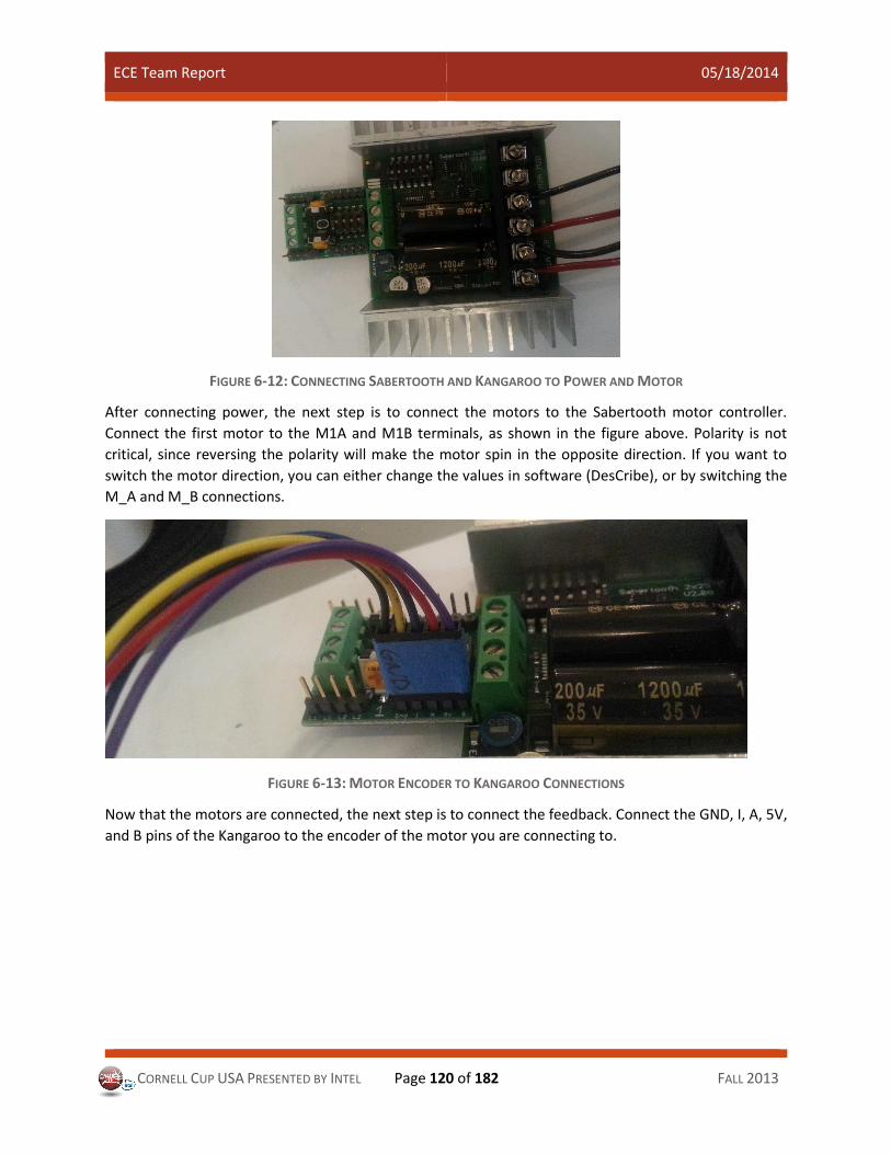
ECE Team Report 05/18/2014
CORNELL CUP USA PRESENTED BY INTEL Page 120 of 182 FALL 2013
FIGURE 6-12: CONNECTING SABERTOOTH AND KANGAROO TO POWER AND MOTOR
After connecting power, the next step is to connect the motors to the Sabertooth motor controller.
Connect the first motor to the M1A and M1B terminals, as shown in the figure above. Polarity is not
critical, since reversing the polarity will make the motor spin in the opposite direction. If you want to
switch the motor direction, you can either change the values in software (DesCribe), or by switching the
M_A and M_B connections.
FIGURE 6-13: MOTOR ENCODER TO KANGAROO CONNECTIONS
Now that the motors are connected, the next step is to connect the feedback. Connect the GND, I, A, 5V,
and B pins of the Kangaroo to the encoder of the motor you are connecting to.
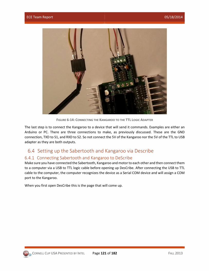
ECE Team Report 05/18/2014
CORNELL CUP USA PRESENTED BY INTEL Page 121 of 182 FALL 2013
FIGURE 6-14: CONNECTING THE KANGAROO TO THE TTL LOGIC ADAPTER
The last step is to connect the Kangaroo to a device that will send it commands. Examples are either an
Arduino or PC. There are three connections to make, as previously discussed. These are the GND
connection, TXD to S1, and RXD to S2. So not connect the 5V of the Kangaroo nor the 5V of the TTL to USB
adapter as they are both outputs.
Setting up the Sabertooth and Kangaroo via Describe 6.4.1 Connecting Sabertooth and Kangaroo to DeScribe Make sure you have connected the Sabertooth, Kangaroo and motor to each other and then connect them
to a computer via a USB to TTL logic cable before opening up DesCribe. After connecting the USB to TTL
cable to the computer, the computer recognizes the device as a Serial COM device and will assign a COM
port to the Kangaroo.
When you first open DesCribe this is the page that will come up.

ECE Team Report 05/18/2014
CORNELL CUP USA PRESENTED BY INTEL Page 122 of 182 FALL 2013
FIGURE 6-15: DESCRIBE STARTING PAGE
Click Connect and Download Settings. Then next page that will come up is shown below.
FIGURE 6-16: CHOOSING AND SETTING THE SABERTOOTH AND KANGAROO
In the figure above we see that there are three options in the Connect window. Serial Port, Baud Rate and
Address. In this case the serial port assigned to the kangaroo was COM 6. The default baud rate is 9600
and the default address is 128. Leave these alone for now and click ‘Ok’. When the download works the
window that comes up is shown below.

ECE Team Report 05/18/2014
CORNELL CUP USA PRESENTED BY INTEL Page 123 of 182 FALL 2013
FIGURE 6-17: DOWNLOADING SETTINGS FOR THE FIRST TIME (NECESSARY IF YOU WANT TO COMMUNICATE BETWEEN
DESCRIBE SOFTWARE AND THE HARDWARE)
Note: Sometimes when you click OK or Connect and Download Settings, the window that will show up is
the one below, where the error message is “Failed to open serial port.” Don’t panic. Just click OK and click
the Connect and Download Settings button that is located on the top left hand corner of the screen under
“File”. Sometimes this message comes up repeatedly. Just continue clicking Connect and Download
Settings.
FIGURE 6-18: DESCRIBE COMMUNICATION GLITCH

ECE Team Report 05/18/2014
CORNELL CUP USA PRESENTED BY INTEL Page 124 of 182 FALL 2013
The other message you could (but should not) get is shown below:
FIGURE 6-19: WRONG ADDRESS OR BAUD
If you get the message above, it means that somewhere in the initial settings there is an error and you
have either the wrong baud rate or the wrong address.
6.4.2 Optimization of Settings for Sabertooth and Kangaroo via DeScribe
FIGURE 6-20: OPTIMIZING SABERTOOTH AND KANGAROO COMMUNICATION
In order to get optimal performance with your Kangaroo, after you have followed Section 6.4.1
("Connecting Sabertooth and Kangaroo to Describe") click on the serial tab as shown above and change
the Baud Rate by clicking that dropdown menu and clicking on 115200. Do the same thing for the
Sabertooth Baud Rate by clicking on the dropdown menu and clicking on 19200. This makes sure that the
Kangaroo and the Sabertooth are communicating with each other and other devices on their fastest
setting. After doing so click on 'Upload Settings on Device' which is located beside the 'Connect and
Download Settings' option. Turn off and turn on the Sabertooth to ensure the settings have taken effect.
Change to 115200
Change to 19200
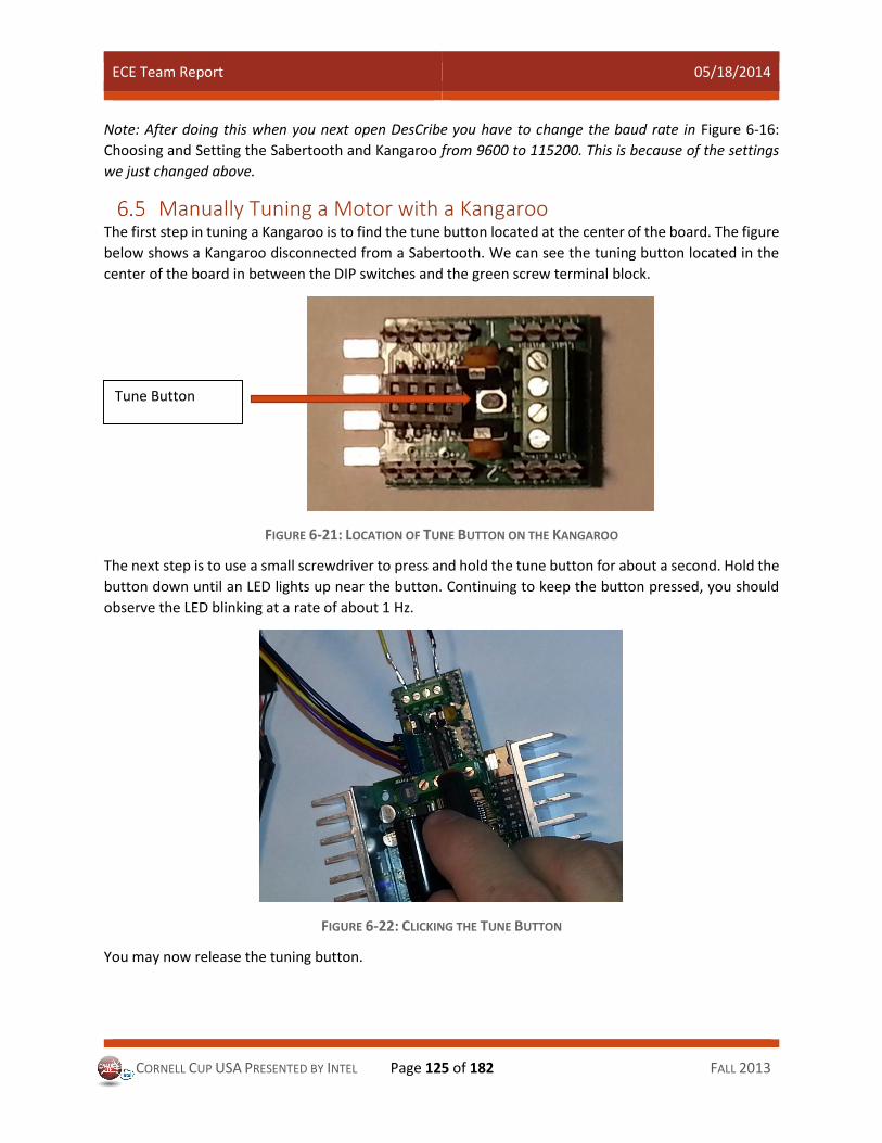
ECE Team Report 05/18/2014
CORNELL CUP USA PRESENTED BY INTEL Page 125 of 182 FALL 2013
Note: After doing this when you next open DesCribe you have to change the baud rate in Figure 6-16:
Choosing and Setting the Sabertooth and Kangaroo from 9600 to 115200. This is because of the settings
we just changed above.
Manually Tuning a Motor with a Kangaroo The first step in tuning a Kangaroo is to find the tune button located at the center of the board. The figure
below shows a Kangaroo disconnected from a Sabertooth. We can see the tuning button located in the
center of the board in between the DIP switches and the green screw terminal block.
FIGURE 6-21: LOCATION OF TUNE BUTTON ON THE KANGAROO
The next step is to use a small screwdriver to press and hold the tune button for about a second. Hold the
button down until an LED lights up near the button. Continuing to keep the button pressed, you should
observe the LED blinking at a rate of about 1 Hz.
FIGURE 6-22: CLICKING THE TUNE BUTTON
You may now release the tuning button.
Tune Button

ECE Team Report 05/18/2014
CORNELL CUP USA PRESENTED BY INTEL Page 126 of 182 FALL 2013
FIGURE 6-23: STATUS LIGHT
As you can see in the picture above there is a light blinking. This is the status light. After holding down the
tune button the status light will periodically blink once. You can continue to cycle through the frequency
of these blinks by tapping the tune button shown at the beginning of this section. So tapping the button
again would make the light blink twice, tapping it again would make the light blink thrice, and tapping it
again would take you back to one blink. For our case we want the status light to only blink once. Once you
have it blinking periodically once, tap and hold the tune button until you see rapid blinks you are now
ready to tune the motor connected to the kangaroo.
To tune the motor, first turn the motor clockwise 180 degrees by hand. While you are rotating the motor,
the orange light on the Kangaroo near the tune button should be solid orange. Once you reach 180
degrees, stop.
FIGURE 6-24: ROTATING THE MOTOR CLOCKWISE
Status Light

ECE Team Report 05/18/2014
CORNELL CUP USA PRESENTED BY INTEL Page 127 of 182 FALL 2013
Now we want to turn the motor 360 degrees in the opposite (counter-clockwise) direction. Using your
hand again, spin the motor in the counter-clockwise direction 180 degrees back to the start, then an
addition 180 degrees past the start. Once you have rotated the motor a total of 360 degrees, stop.
FIGURE 6-25: ROTATING THE MOTOR COUNTERCLOCKWISE
The final step is to turn the motor back to the start. To do this, rotate the motor 180 degrees in the
clockwise direction. Once you have rotated the 180 degrees, back away from the motor, and click the
tune button on the Kangaroo. The motor will spin on its own to find tuning parameters. Once it is
finished, power cycle the Sabertooth/Kangaroo. The motor is now tuned and ready for simple serial
commands.
FIGURE 6-26: ROTATING THE MOTOR BACK TO HOME POSITION
Note: In this documentation we have shown how to manually turn the motor by hand to tune the motor. In
real-life, you should ideally be turning the motor in the actual system. For example, when tuning R2-I2, we

ECE Team Report 05/18/2014
CORNELL CUP USA PRESENTED BY INTEL Page 128 of 182 FALL 2013
rolled him forward, then backward, then forward again. This provides optimal tuning, since the motor has a
realistic load.
Tuning a Specific Motor with a Kangaroo via DeScribe In this section we shall describe how to tune motors that cannot be tuned manually because of their high
torque. There is a way to tune motors using DesCribe, whichcan be used for all motors and is preferred to
manual tuning. First click on the ‘Live Test’ option which is under the “Upload Settings to Device.”
FIGURE 6-27: LIVE TEST AND TUNE OPTIONS
Once you are in the ‘Live Test’ option click Tune, a window will pop up as shown below. On that window
click ‘Begin’. Highlight and click Teach Distance as shown below.
FIGURE 6-28: SETTING UP FOR TUNING
Once you have highlighted and clicked Teach Distance the greyed out Slide Bar for Channel 1 and Channel
2 will become available as shown in Figure 6-29.

ECE Team Report 05/18/2014
CORNELL CUP USA PRESENTED BY INTEL Page 129 of 182 FALL 2013
FIGURE 6-29: GOING IN ONE DIRECTION WITH THE MOTOR
Once you have access to the slidebars, you can move them to either the right or the left. Doing so will
move the motor either clockwise or counterclockwise, respectively. Once you have clicked and dragged
the slider to the right you have to hold it there until the motor has moved for 180 degrees. This is just like
manual tuning except that you don’t have to physically move the motor.
FIGURE 6-30: GOING IN THE OTHER DIRECTION
Once you have moved the motor for 180 one way let go of the mouse and then click and drag the mouse
to the other direction until you have gone 360 degrees. This is just like manual tuning. You can do this for
both Channel 1 and Channel 2 if you have two motors connected to the Kangaroo and Sabertooth. After
you have gone the distance, you want to come back to home and therefore must go back 180 to the base
position, as shown in Figure 6-31.

ECE Team Report 05/18/2014
CORNELL CUP USA PRESENTED BY INTEL Page 130 of 182 FALL 2013
FIGURE 6-31: GOING BACK TO BASE POSITION
Once you have set the boundaries for the motors hit ‘Continue’ option on the screen. All the options will
be greyed out and the motor should start tuning.
FIGURE 6-32: CONTINUE TUNING. MOTOR TUNING SHOULD TAKE PLACE
If for some reason the tune stops midway and you see the error message, “Limit Switches Reached”, redo
the tune and this time instead of going 180 degrees, go 360 degrees in one direction, 720 degrees for
going the second way (360 back and 360 the other way) and then 360 the first direction to come back to
the starting point.
After the motor(s) has tuned you need to power cycle and then download settings from device. This gives
you all the settings from the tuned motors and allows you to save and ensure that the device has tuned.
6.6.1 Tuning Environment Upon starting an automatic tuning with either the tune button on the Kangaroo or through DesCribe, the
motor will begin to aggressively shake and spin at fast speeds. This is normal, and is how the motor
controller determines which parameters to use. This brings up an important tradeoff to consider when
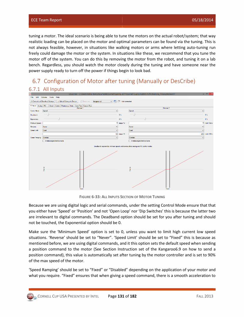
ECE Team Report 05/18/2014
CORNELL CUP USA PRESENTED BY INTEL Page 131 of 182 FALL 2013
tuning a motor. The ideal scenario is being able to tune the motors on the actual robot/system; that way
realistic loading can be placed on the motor and optimal parameters can be found via the tuning. This is
not always feasible, however, in situations like walking motors or arms where letting auto-tuning run
freely could damage the motor or the system. In situations like these, we recommend that you tune the
motor off of the system. You can do this by removing the motor from the robot, and tuning it on a lab
bench. Regardless, you should watch the motor closely during the tuning and have someone near the
power supply ready to turn off the power if things begin to look bad.
Configuration of Motor after tuning (Manually or DesCribe) 6.7.1 All Inputs
FIGURE 6-33: ALL INPUTS SECTION OF MOTOR TUNING
Because we are using digital logic and serial commands, under the setting Control Mode ensure that that
you either have ‘Speed’ or ‘Position’ and not ‘Open Loop’ nor ‘Dip Switches’ this is because the latter two
are irrelevant to digital commands. The Deadband option should be set for you after tuning and should
not be touched, the Exponential option should be 0.
Make sure the ‘Minimum Speed’ option is set to 0, unless you want to limit high current low speed
situations. ‘Reverse’ should be set to “Never”. ‘Speed Limit’ should be set to “Fixed” this is because as
mentioned before, we are using digital commands, and it this option sets the default speed when sending
a position command to the motor (See Section Instruction set of the Kangaroo6.9 on how to send a
position command), this value is automatically set after tuning by the motor controller and is set to 90%
of the max speed of the motor.
‘Speed Ramping’ should be set to “Fixed” or “Disabled” depending on the application of your motor and
what you require. “Fixed” ensures that when giving a speed command, there is a smooth acceleration to

ECE Team Report 05/18/2014
CORNELL CUP USA PRESENTED BY INTEL Page 132 of 182 FALL 2013
the maximum acceleration limit, while “Disabled” does not have a ramping when giving a speed
command. Note that this option is only applied to the speed command and not to the position command.
‘Single Direction’ option should be checked if you only want your motor to spin in one set direction.
6.7.2 Analog and RC and Serial (Explanation about Design Specs) We do not use Analog Settings nor do we use RC settings in our design. This is because our overall design
is simple control at the low level using serial commands. We then implemented all high level logic at the
CS level. Thus we were able to do digital control at the low level and ensure that it could be controlled by
higher level logic. Serial settings have been described in Section 6.4.2.
6.7.3 Control
FIGURE 6-34: CONTROL SECTION OF MOTOR TUNING
The settings ‘Position Deadband’ and ‘Speed Deadband’ should be set automatically after motor tuning.
The option ‘Cut power when stopped’ will send a Powerdown command (see Section 1.8 when you send
a speed command to 0. The option ‘Hold position once stopped’ will ensure that the motor controller will
very precisely hold its current position when a speed command to 0 is sent, otherwise it will loosely hold
the position and will not lock the motor. The position is always held precisely after a position command is
executed regardless of whether the option is checked or not.
The advanced section is set up automatically after tuning. Do not mess with it unless you want to flip the
logical forward and backward directions, which is described in the next section.
6.7.4 Flipping the logical forward and backward directions If you would like to flip the logic forward and backward you must do two things together and they must
be done very carefully:

ECE Team Report 05/18/2014
CORNELL CUP USA PRESENTED BY INTEL Page 133 of 182 FALL 2013
1. Turn off all power to the system, Flip the motor power lines (the physical wires shown in Figure
6-12: Connecting Sabertooth and Kangaroo to Power and MotorFigure 6-12)
2. Turn on the power, but do not send the start command. Go to DesCribe, under Control in
subsection Advanced, change the state of the inverted setting under the right channel. After you
have done so click ‘Upload settings do device’ to upload the settings to the kangaroo.
If you do not do these two steps properly, and you send a command to the motor, the motor will have
reversed feedback and take off at full speed if you send a command which could potentially damage the
motor or the whole system.
6.7.5 Positioning
FIGURE 6-35: POSITIONING SECTION OF MOTOR TUNING
When you first send a ‘Home’ command (See Section 6.9) everything is set to 0. Some motors have an
index pulse, and in order to use these index pulses, you must change the setting from ‘Use home position’
to ‘Use first encountered index pulse/home switch (Normally Closed)’. The option homing has to say home
until interrupted.
“Machine Zero” has sets the offset of the user defined 0 after homing. This is used if in case you want to
offset the homing position of the index pulse.
“Homing speed” is to set the speed the motor goes to home at.
“Homing time out” is to set the time the motor should maximum take to reach home from the limit switch.

ECE Team Report 05/18/2014
CORNELL CUP USA PRESENTED BY INTEL Page 134 of 182 FALL 2013
To use limit switches, under the section “Origin” the option ‘Use home position’ should be clicked. Under
the section “Homing” make sure ‘Use limit switches’ is selected. The section at the very bottom “Limit
Switches (Normally Closed)” should have ‘Use limit switches’ selected and if you are using one limit switch
only select the option to do so which is under the ‘Use limit switches’. Above that are two options “Use
Hard Limit Switch” and “Use Soft Limit Switch”.
Hard limits are limits that cut power to the motor when you have reached a certain distance and require
a Start and Home Command (see Section 6.8) to restart. Using hard limits is not recommended.
Soft limits control the speed of the motor and ensure that the motor stops at the exact distance. This is
much more precise and does not require a Start or home command.
The section “Nominal Travel” is not relevant for digital control and is not used in this case.
Sending Simple Serial Commands to Kangaroo via PuTTy After following Sections 6.3 to 6.7 you are now ready to send simple commands to move your motor via
PuTTy. If you know your COM port (can be found under devices in the Control Panel), and you know the
baud rate of the Kangaroo (Section 6.4.2) you can use PuTTy to send serial commands that can control
your motor.
Before sending commands with PuTTy, we need to configure some options within PuTTy. On the left side
of PuTTy, click “Terminal.” When the screen seen below appears, verify that “Force on” is selected for
both “Local echo” and “Local line editing.” This will enable us to see what we are typing in the PuTTy
terminal.
FIGURE 6-36: MAKING SURE "LOCAL ECHO" AND "LOCAL LINE EDITING" ARE BOTH "FORCE ON"
Now that we have configured the options in PuTTy, we need to next configure the session options. Under
“Connection type,” select the “Serial” option. Under “Serial line,” the word COM should appear with a
number. Verify that this is the correct COM port by going to device manager in Windows. Once the correct
COM port has been entered, next set the connection speed. If you want, you can save this session for later

ECE Team Report 05/18/2014
CORNELL CUP USA PRESENTED BY INTEL Page 135 of 182 FALL 2013
by typing a name into the “Saved Sessions” box, then clicking the “Save” button to the right of the window.
When opening PuTTy in the future, you can select a saved session and click the “Load” button to load your
session. Hit the “Open” button on the bottom of the PuTTy window to open the session.
FIGURE 6-37: SETTING UP KANGAROO FOR SERIAL COMMUNICATION VIA PUTTY
Instruction set of the Kangaroo For more information, please view pages 12-15 from the Kangaroo datasheet
(https://www.dimensionengineering.com/datasheets/KangarooManual.pdf )
In our case the motors are run in independent drive, which means that motor 1 is independent from motor
2. This is done to achieve more precise movement. All commands are sent as ASCII characters via PuTTy
(Section 6.8) and no spaces are necessary. To complete any command, you must send a carriage return
and new line: ‘\r\n’. The robot will read and execute only the last command sent to it. So if you send a
position command and then immediately send a speed command, the position command will be ignored
and the motor will just hold the speed command indefinitely. Verification commands do not interrupt
anything; they can be sent at any time.
6.9.1 Motor Command Explanation Upon setting up a connection to the Kangaroo, a list of commands need to be sent before sending velocity
or position commands. The first thing that needs to be sent is a start command, which looks like this:
1, start
The first command to be sent to the Kangaroo must be a start command, since all commands sent to a
channel are ignored before a start command. Looking at the Kangaroo, you can see that there are two
sides. One is labeled “1,” and the other is labeled “2.” If you are using one motor, make sure you send
commands to the right channel. If using both channels, then be sure to start channel 2 as well.
After starting the channel, the next task is to declare units. The format of the command is:

ECE Team Report 05/18/2014
CORNELL CUP USA PRESENTED BY INTEL Page 136 of 182 FALL 2013
1, units 1000 thousandths = 1024 lines
The units command is used to change the input from volts/encoder lines to a user defined unit. You must
use whole numbers in your command.
After declaring units, you next want to home the motors using the home command. Sometimes you do
not want to use units and can just skip to the next command for testing purposes.
1, home
This command moves the motor back to its home position.
Now that the motor is homed, it is good practice to verify that the motor is at position 0. This can be
checked by using a getp command.
1, getp
After sending these commands, the motor is ready for speed and position commands
Sending speed and position commands
To send a speed command to a motor, the format is
1, sXXX (e.g. 1, s100)
Be careful when sending speed commands, as the motor will continue to spin at this speed until you
command it to stop. Start from small speeds and work your way up. Sending a fast speed can cause
damage to your robot and motors.
To send a position command to a motor, the format is:
1, pXXX (e.g. 1, p100)
When sending a position command by itself, you should take caution since if you do not change any
maximum speed settings through describe software, then the motor will spin to the commanded position
at the maximum speed.
In order to spin the motor to a particular position at a particular speed, a mixed command can be used.
An example of a mixed command is:
1, p0 s5000
This command will make the motor travel to position 0 at a speed of 5000.
Finally, another useful command is the power down command. The powerdown command turns off the
motor and control system. You are still able to read position and speed after powering down. This can be
used to save power or allow the motor to free-spin.
1, powerdown

ECE Team Report 05/18/2014
CORNELL CUP USA PRESENTED BY INTEL Page 137 of 182 FALL 2013
Note: All commands can be used with either Channel 1 or Channel 2, to control motor 2 substitute the 1
that prefaces all commands with at 2. For example we have “1, getp…” we can change that to “2,
getp”; this is true for all commands that have been listed above and in the reference documentation listed.
6.9.2 Motor Command Examples Initialization commands
The sequence of commands used when first turning on the robot:
Initialize motor 1 ............................................................................ 1, start
Initialize motor 2 ............................................................................ 2, start
Zero the absolute position of motor 1 ........................................... 1,home
Zero the absolute position of motor 2 ........................................... 2,home
Verify position of motor 1 .............................................................. 1,getp (receive P1,0)
Verify position of motor 2 .............................................................. 2,getp (receive P2,0)
Verify speed of motor 1 ................................................................. 1,gets (receive S1,0)
Verify speed of motor 2 ................................................................. 2,gets(receive S2,0)
Position commands and speed commands
X & Y represents the value for position or speed. It can be positive or negative.
These commands can also be sent to motor 2. Change the first number to a 2 in every command.
Move to absolute position X (using default speed) ....................... 1,pX
Move to absolute position X at speed Y ........................................ 1,pXsY
Move at absolute speed X.............................................................. 1,sX
Move forward/backward distance X .............................................. 1,piX
Move forward/backward distance X at speed Y ............................ 1,piXsY
Increase/decrease speed by X ....................................................... 1,siX
*Shutdown motor & cut power immediately ................................ 1,powerdown
More Verification Commands
These commands can also be sent to motor 2. Change the first number to a 2 in every command.
Verify distance moved since last command .................................. 1,getpi (receive P1,X)
Verify speed change since last command ...................................... 1,getsi (receive P2,X)
NOTE: All verification commands will return a string using uppercase ‘P’ or ‘S’ when the motor has
completed its speed or position command, and a lowercase ‘p’ or ‘s’ when the motor is STILL in the process
of getting to that speed or position. There is a difference in case.
Example code. Received commands are italicized and indented.
//INITAILIZE THE ROBOT
1, start
2, start

ECE Team Report 05/18/2014
CORNELL CUP USA PRESENTED BY INTEL Page 138 of 182 FALL 2013
1, home
2, home 1, getP
2, getP
Pause()……..
P1,0
P2,0
//MOVE FORWARD 100 units
1, p100
2, p100
//VERIFY
1, getp 2, getp
P1,100
P2, 100
//MOVE BACKWARDS 50units at 30units/s
1, p-50s30
2, p-50s30
Pause()…..
//SPIN A DISTANCE OF 50units
1, p50 2, p-50
Pause()…..
//RAMP UP SPEED
1, s1 or 1,pi1000s1 or 1,si1
1, s2 or 1,pi1000s2 or 1,si1 1, s3 or 1,pi1000s3 or 1,si1
1, s5 or 1,pi1000s5 or 1,si2
1, s10 or 1,pi1000s10 or 1,si5
etc etc etc etc
Calculations of ticks and distances setting up Units One of the commands that we mentioned above and will discuss in this section is ‘units’. Each motor has
a different number of ticks per rotation and this can be figured out from the documentation of the motor.
The specification heading you want to look for are “Counts per turn” and “Reduction”. Once you get both
you multiply them together to get an accurate units per rotation. This can be set up as follows. Suppose
you have 3883 ticks per turn; to set up so that when you type 1, p1 and get one rotation from this
command, you have to type after the startup command and home command: 1, units 1 = 3883. If we want
to divide this rotation into 100 even divisions we set the command: 1, units 100 = 3883.

ECE Team Report 05/18/2014
CORNELL CUP USA PRESENTED BY INTEL Page 139 of 182 FALL 2013
6.10.1 Setting up Units in DesCribe Instead of always setting up units command in the PuTTy screen during operation you can set the units in
DesCribe software and they will be permanent for that setting. After setting up all configurations and units
you can upload this to the Kangaroo, run PuTTy and do not have to worry about setting up units. As you
can see in the figure below, there is the left hand side of the equation and the right hand side. The left
hand side of the equation is how many divisions you would like to divide the number of ticks per rotation.
The right hand of the equation is how many ticks per unit you have. This can be calculated and set by the
user.
FIGURE 6-38: SETTING UP UNITS IN DESCRIBE
We refer to Figure 6-38 to explain how to calculate distances and get units in ticks per distance. Here we
have 1850 ticks per rotation, and our wheel has a circumference of 4.71(2*radius of wheel* π) inches.
So to get total lines/ticks per inch we divide the ticks per rotation by the circumference of the wheel to
the total of 392.78 ticks per rotation, however we round up because the command only takes in whole
number values.
Error Messages and their fixes. Kangaroo Error Codes
When communicating with a Kangaroo over PuTTy, the Kangaroo may print error codes to your terminal
session. The listing of error codes is shown in the figure below:

ECE Team Report 05/18/2014
CORNELL CUP USA PRESENTED BY INTEL Page 140 of 182 FALL 2013
FIGURE 6-39: ERROR TABLE AND EXAMPLES OF ERRORS
E1
Receiving an E1 code means that you have tried sending commands to the Kangaroo before sending a
start command. To resolve this error, start the motor channels you are using. This can be done with
1, start
E2
Receiving an E2 error code means that you have started the channel, but have not homed the motor. If
you do not home the motor, then absolute position commands are meaningless. In order to home a
motor, use the home command
1, home
e2

ECE Team Report 05/18/2014
CORNELL CUP USA PRESENTED BY INTEL Page 141 of 182 FALL 2013
In addition to the E2 error, there is also an e2 error. If you see this error, then you have tried sending a
command while the homing is in progress. In order to resolve this error, simply wait until the motor is
homed before sending additional commands.
E3
This is an error you will receive a lot. E3 occurs when the feedback is broken, or when a tune did not go
through properly. In order to resolve E3, first verify that the wiring is setup correctly between the motor’s
encoder and the Kangaroo. After verifying proper electrical connections, the next step is to redo the tune
if the error still persists. After finishing the tune, don’t forget to powercycle the Kangaroo. Failing to turn
off power after the tune, then turning power back on will cause an E3 to appear.
E4
The E4 error appears when you have tuned a motor, but then moved either the 2nd or 4th DIP switch. In
order to resolve this error, you must either put the 2nd and 4th DIP switches back to the state that they
were in during the tuning, or redo the tuning.
E5
The E5 error appears when you enter an invalid command that is not recognized by the Kangaroo. Double-
check your commands for typos, or refer to the Kangaroo manual to verify that your command is valid
and has the correct syntax.
E6
This is the final error that the Kangaroo will print to the PuTTy terminal. E6 appears when the Kangaroo
loses communication with the PC or microcontroller since the last command. To resolve this error, confirm
that wires have not come lose or shorted with other wires.
Note: Refer to section 4.1 for information on how to deal with potential current spikes from the
motor starting up and switching directions, without relying upon motor controllers.
I-3P0 Walking Control The I-3P0 walking mechanism was controlled by the ATmega 2560 microcontroller on the Arduino Mega
2560 board. The purpose of the circuit was to control the weight shifting by controlling the torso motor
so as to enable the robot to walk stably, along with sending the correct walking command to the motor
controller at the right time. To increase reliability, control was done at a completely low level by direct
low-level register access of the Arduino Mega microcontroller: the ATmega 2560.
The ATmega peripherals/modules used for the weight shifting control are:
The 16-bit Timer 3 controls the main timing for the weight shifting.
The 16-bit Timer 1 is used as the time base for the PWM channel used to drive the piezoelectric
speaker (buzzer).
The Compare module associated with the 16-bit Timer 1 – as the PWM module.
The UART0 module for communicating with the computer. This was used extensively during
design and testing, especially for debugging.

ECE Team Report 05/18/2014
CORNELL CUP USA PRESENTED BY INTEL Page 142 of 182 FALL 2013
The UART2 module to communicate with the Kangaroo motor controller for control of the torso
motor for weight shifting.
The IO module for motor braking control.
6.12.1 Torso Motor Motion The requirement for control is that the torso motor starts at the left (corresponding to a position -550 for
the motor controller), accelerates constantly to the middle (corresponding to a position 0 for the motor
controller) and then decelerates constantly to the right (corresponding to a position 550 for the motor
controller), then accelerates constantly to the middle before decelerating to the left and so on. During
this time, when the motor is at the center (and moving at maximum speed), a walk step is initiated – i.e.
a foot is lifted off the ground. The foot lands onto the ground when the motor is again at the center. This
is when the other leg is raised off of the ground to initiate another walk sequence (if required). Before
initiating a walk sequence, the motor brakes are released and the brakes are engaged after the walk
sequence is completed. A buzzer starts beeping before the walk sequence is initiated.
The weights that are shifted from side to side to provide the counterbalance for the robot while walking
are attached to the torso motor that moves from side to side. The control is done by the microcontroller
via timing (using the internal 16-bit timer 3). Therefore, the walk sequence consists of both the torso
motor motion providing the counterbalance as well as the main walking motor.
The task of the microcontroller here in terms of motor control was to set up the parameters for the motor
controller: the speed and position control. In other words, motor control was done by the motor
controllers themselves – the microcontroller was used to control what speed setting and position setting
to use and the motor controller used that setting to control the motor.
6.12.2 Calculations It was determined that the average walking speed was to be around 1.5 steps per second. Speed control
was to be done in 32 steps. The timer 3 was set to interrupt every 20.624ms. Every timer interrupt, the
speed was incremented. This was done by precalculating a speed table (with 32 entries) that
approximated a triangular waveform (first 15 linearly ramp up, 2 constant at the peak value, and then the
final 15 linearly ramp down) to obtain constant acceleration followed by constant deceleration. Thus the
total time for a single step was:
32 ∗ 20.624 ∗ 10−3𝑠𝑒𝑐𝑜𝑛𝑑𝑠 = 0.66 𝑠𝑒𝑐𝑜𝑛𝑑𝑠
This gave:
1 𝑠𝑡𝑒𝑝𝑠
0.66 𝑠𝑒𝑐𝑜𝑛𝑑𝑠= 1.51 𝑠𝑡𝑒𝑝𝑠/𝑠𝑒𝑐𝑜𝑛𝑑
Every timer interrupt, the speed was updated by incrementing the value of the table pointer to the speed
array/table and then sending this information over to the motor controller. After all updates, the pointer
was reset to start over.
The speed array was calculated as follows. The nth entry in the table (Tn) for 0 ≤ n ≤ 15 was calculated as:
𝑇𝑛 =(𝑛 + 1) ∗ 𝑆𝑝𝑒𝑒𝑑𝑚𝑎𝑥
16, 0 ≤ n ≤ 15

ECE Team Report 05/18/2014
CORNELL CUP USA PRESENTED BY INTEL Page 143 of 182 FALL 2013
The first 16 entries were “mirrored” to obtain the last 16 entries. T17 was given the value of T16, T18 was
given the value of T15, T19 was given the value of T14 and so on …. T31 was given the value of T0.
To calculate Speedmax :
𝐷𝑖𝑠𝑡𝑎𝑛𝑐𝑒 𝑓𝑟𝑜𝑚 𝑙𝑒𝑓𝑡 𝑡𝑜 𝑟𝑖𝑔ℎ𝑡 = 11 𝑖𝑛𝑐ℎ𝑒𝑠
𝑑𝑖𝑠𝑡𝑎𝑛𝑐𝑒 = 0.5 ∗ 𝑆𝑝𝑒𝑒𝑑𝑚𝑎𝑥 ∗ 𝑡𝑖𝑚𝑒
With a required time of 0.66 seconds for the torso motor/weight to move from left to right (or from right
to left) [= time for one step] and a distance of 11 inches, this gave a maximum speed of 33.33 inches per
second. This corresponded to the value 3333 for the motor controller and this is the value used in the
code.
6.12.3 Timer Settings The specific timer settings were:
Timer 3 was set to operate in fast PWM mode (Mode 15). This allowed the use of a configurable
period.
The period register was selected as OCR3AH:OCR3AL and was given the value 0x0508, which
along with the prescale value of 1:256 gave a timer interrupt period of 20.624 ms.
Interrupt upon compare match was enabled for required interrupt (every 20.624 ms).
6.12.4 Serial Port Communication The communication between the Arduino and the motor controller was done over the serial port using
the Simple Serial scheme where data was transferred as strings – series of ASCII characters transmitted
over the serial port (UART module of the ATmega 2560).
To send a byte over the serial port, the Serial.write Arduino function was used. However, this is a
low-level function that was configured to only send one byte of data. By managing separate user buffers,
there was maximum low-level control over the system (which was the aim initially and was why the
Arduino Serial.print and Serial.println functions were avoided).
A 10-element character array was used as the buffer. A function was written to send position command
over serial port to the motor controller. Another function was written to send speed command to the
motor controller.
An example position command to the motor controller is “1,p100”. The position command sending
function accepted as its parameters the channel and desired position setting. So, for the example
command the channel is 1, and the position setting is 100. The function took the position setting numerical
value and calculated the individual digits of the numerical value. Then the individual digits were converted
from the numerical value (1, 0 and 0 for 100) to ASCII (‘1’, ‘0’, and ‘0’ for “100”) by adding 48 (=0x30) to
each of the numerical values – 48 is the offset between the actual digits and their ASCII equivalents: ‘0’ =
48, ‘1’ = 49 …. ‘9’ = 57. Then, these individual ASCII characters were sent one after the other (after sending
‘1’, ‘,’ and ‘p’). The command was completed by sending the new line command. The new line command
was sent by sending a carriage return (=13) followed by a line feed (=10). The speed sending function
worked similarly, accepting a desired speed setting (instead of a position setting) as one of the

ECE Team Report 05/18/2014
CORNELL CUP USA PRESENTED BY INTEL Page 144 of 182 FALL 2013
parameters; and sending a channel comma ‘s’ followed by the speed over the serial port followed by a
new line command.
A second buffer was maintained for sending commands to the walking motor. This was used to send a
position and speed command and worked similarly to the above described functions, the difference being
that both a position setting and a speed setting was sent.
The other portion of serial communication was to receive data. To receive data from the serial port, the
function Serial.read was used. This read one byte of data received from the serial port. (Similar to the
Serial.write function, this function is used as a low-level function.) The received bytes were inspected
and stored in an array only if the current byte received corresponded to a comma, a numerical digit or an
alphabetic letter. The array was then “inspected” to receive just the numerical portion of the received
data and then convert that to a numerical equivalent. So, for example, the string “123” (comprised of the
ASCII characters ‘1’, ‘2’ and ‘3’) is converted to the numerical equivalent 123 (a number). This was done
by converting the ASCII characters to numerical digits (by subtracting 48 as explained above) and then
multiplying and accumulating: 1*100 + 2*10 + 3*1 = 123.
A function for getting speed and another for getting position sent commands to the motor controller
asking for current speed or position (as required) and then inspected the received information, processing
it as mentioned above to retrieve the required speed or position information.
6.12.5 Buzzer The piezoelectric buzzer selected has a resonant frequency of about 2500 Hz. Timer 1 is used as the time
base for the PWM. The TOP (set by ICR1AH:ICR1AL) is set to 0x031F (=80010) with a prescaler 1:8. The
duty cycle register (set by OCR1AH:OCRA1L) is set to 0x0190 (=40010). This sets the required frequency
for the buzzer. The output is sent on to pin 11 on the Arduino board. Turning the timer on makes the
buzzer beep and turning the timer off stops the buzzer from beeping. Before starting a walk sequence,
the buzzer is made to beep four times – buzzer stays on for 200ms and stays off for 200ms. This is to alert
anyone near the robot that the robot is about to start walking.
6.12.6 Motor Break The motors had a motor brake winding. When voltage is applied to the brake winding, the brake is
released. Otherwise, by default, the brakes are engaged. In order to do this, a motor brake control system
was designed. In order to ensure sufficient current handling at a high efficiency and simple drive, MOSFETs
were chosen as the switches to control the brake winding. To ensure proper drive of the MOSFET gates,
dedicated low-side MOSFET drivers were used. The system thus essentially consists of MOSFET drivers
(whose inputs are driven by the Arduino or any other input) driving MOSFETs that drive the loads (brake
windings in our circuit). Since the motor winding is of inductive nature, to prevent inductive kickback when
the MOSFET turns off, a flyback diode is employed for each channel. The entire motor brake system
consists of four of these identical channels. While only two channels are used in I-3P0, having two other
channels is good as spare channels.
The MOSFET drivers are powered off of a 12V supply while the motor brake windings (the “load”s) each
have their own drive voltage connection – allowing them to be driven at a desired voltage that is also
within the acceptable VDS(max) voltage range (with headroom) for the MOSFETs (in our robot, it was 24V
and this was more than safe enough for the chosen MOSFETs). The four inputs to the driver circuit are all

ECE Team Report 05/18/2014
CORNELL CUP USA PRESENTED BY INTEL Page 145 of 182 FALL 2013
active high and 5V logic compatible – they were driven directly from the Arduino IO in our robot. In our
circuit, driving an input high released the brake and driving the input low engaged the brake.
MOSFETs were chosen such that they had a relatively high VDS(max) rating to allow the use of higher
voltages. The other crucial parameter was the RDS(on). Having a low RDS(on) meant higher efficiency due
to lower power dissipation; this also meant that no heatsink was required for relatively low currents as in
our circuit.
The schematic and PCB were designed using PCB Artist software supplied by Advanced Circuits. The PCB
was fabricated by Advanced Circuits. The PCB design was done so as to minimize physical size. The
schematic and PCB for the motor brake system are shown below.
FIGURE 6-40: PCB FOR MOTOR BRAKE SYSTEM

ECE Team Report 05/18/2014
CORNELL CUP USA PRESENTED BY INTEL Page 146 of 182 FALL 2013
FIGURE 6-41: SCHEMATIC FOR MOTOR BREAK SYSTEM

ECE Team Report 05/18/2014
CORNELL CUP USA PRESENTED BY INTEL Page 147 of 182 FALL 2013
6.12.7 Final Walking Sequence Turn on buzzer. Beep 4 times with 0.2s on and off times. Then turn off buzzer.
Initialize the torso motor (responsible for weight shifting).
Initialize the walking motor.
Have a 7 second delay to allow the torso motor to come back to its initial leftmost ‘home’ position.
Let go of the brakes. This means sending logic high to the brake control system.
Send a position command to the torso motor controller to send the motor to the position -550.
This is 5.5 inches to the left of the center of the torso (and is a bit to the right of the leftmost
‘home’ position which is at a position of about -570).
Wait a second. This ensures that the motor reaches position -550.
Start the walking control.
o This means that the weight shifting control starts to shift the weight from left to right to left
and so on.
o Whenever the weight is at the center, a new walk step is taken. The number of steps required
is sent to the motor controller as (100 * number_of_steps). The motor controller for the
walking control is calibrated such that 1 step corresponds to a position of 100. This command
is only sent the first time and not after that.
o The weight shifting happens as many times as required: (number_of_steps + 1) and the
weights always end up at the left.
Wait two seconds.
Engage the brakes by sending logic low to the brake board.
All the code use for testing and executing walking can be found in Appendix B: I-3P0 walking code.
7 Servo Motors A servo motor is a device which combines an electric motor and a motor driver into a single device. The
motor is the physical magnets and bearings which spin a shaft, and the motor driver uses a low-level input
signal to control the power to the motor, controlling its speed and direction. Every servo has 3 wires:
power, ground, and signal. There are two main types of servo motors: Continuous Servos, and 180° Servos.
Continuous servo motors spin freely and they use the input control signal to set the speed and direction
of the motor. They are a very low power substitute for a stand-alone motor and dedicated external motor
controller, which would be used in higher power applications. 180° Servos, however, have a
potentiometer built into them, which serves as a position feedback device. This changes the function of
the servo motor into an absolute position controller. It holds a specific position between 0° and 180°,
designated by the control signal, and it does not rotate continuously. These types of servo motors are the
most common and most useful type, and they are the only type used in our project.
Servo Power Supply 7.1.1 Voltage All servo motors are designed to operate with a voltage between 4.8V and 6.0V. A supply voltage of 4.8V
will give the servo a lower torque/power capability than a supply voltage of 6.0V. However, most

ECE Team Report 05/18/2014
CORNELL CUP USA PRESENTED BY INTEL Page 148 of 182 FALL 2013
commercial dedicated power supplies are not available in 6.0V outputs, so it is very common to operate
servos at a standard value of 5.0V.
7.1.2 Current The amount of power drawn by a servo is directly proportional to the load or stress on its arm as it moves.
If it is moving a heavy weight, it will draw more current. The max amount of current a servo can draw is
dependent on the physical size of the servo motor, but it is generally below 1A. Roughly 0.5A is a good
starting approximation for each servo. Therefore when choosing a power supply, it should have a current
output rating equal to at least (0.5 X Number of Servos). Multiple servos can all be powered in parallel as
long as the power supply can output enough current for all of them combined.
7.1.3 Power Spikes and Noise The most important thing to account for when powering a servo motor is its power spikes. The section
below outlines the servo control signal, which has a period of 20ms. When a servo is holding a specific
position, it sends power to the motor every 20ms as well, corresponding directly to the control signal. This
results in large current spikes every 20ms drawn from the power supply. AC/DC power supplies plugged
into a wall outlet are capable of very high current outputs, but they are terrible at enduring current spikes.
If you plug several servos directly into a single AC/DC power supply, they will most likely fail to respond at
all. Fortunately there is a very elegant, simple solution to fix this problem. The power line for all servos
should be connected to a large electrolytic capacitor and a flyback diode between power and ground. If
many servos are connected to a single power supply, they can all share the capacitor and flyback diode.
See section 4.1 for more information on this topic.
FIGURE 7-1: POWER SUPPLY CIRCUIT
The flyback diode is used to dissipate any reverse current spikes that might be emitted from the servo
motors. Any motor is represented as an inductive load, which means it is capable of reverse current spikes,
and so a flyback diode is very standard protection circuitry. A Schottky diode rated for 1A and 40V is very
standard in this application.
The electrolytic capacitor isolates the power supply from the current spikes of the servo motors. It is a
very simple and effective solution that is essential to proper function of a servo. This capacitor should be
“large enough” to isolate all current spikes from the servos. Since the current spike is roughly 1A per servo,
and it lasts roughly 1ms, using the equation 𝐼 ∗ 𝑡 = 𝐶 we can see that the capacitor should be 1000𝜇𝐹
per servo motor, and rated at 2 x operating voltage which would be 2x5V= 10V.

ECE Team Report 05/18/2014
CORNELL CUP USA PRESENTED BY INTEL Page 149 of 182 FALL 2013
Servo Control Signal It is very important to note that there is absolutely no standard specification for a servo control signal.
Each and every servo motor must be tested and calibrated to be used properly as a precise position
controller. However, every control signal is generally a 5V square wave with a 1.5ms duration and a 20ms
period. The full range of the pulse signal is generally 1ms to 2ms, which corresponds to the servo positions
between 0° and 180°. It is not uncommon, however, to use servos with a pulse duration range of 0.5ms
to 2.5ms. By sending a signal with pulse widths within its range, the signal can specify a position between
0° and 180°. The signal corresponds linearly to position degrees, which makes it easy to divide the range
into 180 pulse widths each corresponding to one degree. A microcontroller or a dedicated servo controller
like the Pololu Servo Controller is capable of sending these precise control signals to the servo. The only
way to truly determine the exact range of the servo is to manually calibrate it and test its range.
If a pulse duration outside of its range is sent to the servo, it will attempt to move outside its physical
range of 0° to 180° and lock up at one extreme. This will cause the servo to short circuit, and it will draw
very high currents in excess of 1A. This could damage the power supply used to power them, overheat
the servo motor, or destroy it altogether. Whenever controlling a servo motor, make sure to never send
a control signal outside the servo’s maximum range to avoid locking the servo in an extreme. When
testing, it is important to only allow the servo to lock up in an extreme position for 1 or 2 seconds max.
FIGURE 7-2: EXAMPLE SERVO CONTROL SIGNAL
7.2.1 Signal Buffer The servo motors generate a large amount of electrical noise, which propagates back through the signal
line. If the servo motors are connected to a dedicated servo controller, no other electronics are using
those data lines so there generally is no need to buffer the signal lines. However, when using a custom
programmed microcontroller to control the servo signals, you may find that the signal lines become filled
with electrical noise. The best way to combat this is to use a simple active OpAmp buffer in series with
each signal line between the microcontroller and the servo control line. A Schmitt Trigger buffer is an even
better option, because it will only allow a digital output of 0V or 5V, thereby improving the rise and fall

ECE Team Report 05/18/2014
CORNELL CUP USA PRESENTED BY INTEL Page 150 of 182 FALL 2013
time of the signal. This will help to keep the electrical noise from the servo out of the microcontroller data
signals, including those used for things other than servo control.
Servo Calibration The first thing to do when using a new servo motor is to calibrate it. Each servo operates between different
signal ranges, even if they are the same make and model, so each needs to be calibrated separately. Follow
the steps below to calibrate any servo motor.
1. Plug the servo motor into power and ground, following the guidelines from the Servo Power section
above.
2. Plug the servo signal line into a signal generator of your choice, whether it is a custom coded
microcontroller or a commercial servo controller.
3. Start with a pulse width of exactly 1.5ms. Then physically place your desired servo arm, gear etc. onto
the servo shaft in the position you would like to roughly define as “90° Center.” The arm might not be
perfectly centered at this point, because of the discrete teeth on the servo shaft.
4. Adjust the pulse width in extremely small increments (0.001ms if possible), until the arm is precisely
centered at 90° Center (by visual inspection). Record the exact pulse width corresponding to 90°.
5. Find the pulse width that 0° and 180° are offset from the 90° position. First, add or subtract 0.5ms
from the calibrated 90° pulse width, which should move the servo to roughly 0° and 180°, respectively.
Adjust the offset value until the servo moves to precisely 0° and 180°. You must select only one offset
value to reach both 0° and 180°. For example, the offset must be ±0.520ms, not + 0.520ms and -
0.510ms. This means that the servo might move to 1° and 181° with the final offset value. Record this
offset value.
Now you have an exact pulse width value for 90° (call it X for now), a value for 0° (X - offset) and a value
for 180° (X + offset). The value for 0° is known as the neutral position, and the value of the offset is known
as the range of the servo. We are using this specific calibration procedure because the neutral value and
range value are the two variables that need to be set in the Pololu Servo Controller for each servo to set
its calibration.
Commercial Servo Controller An example of a robust commercial servo controller is the Pololu Servo Controller. They are available in a
range of 6, 12, 18 and 24 servo channels and they all operate with the same protocols and software. They
can also be plugged into a computer using a USB cable, which makes them very easy to interface with and
calibrate servos using their Control Center software.

ECE Team Report 05/18/2014
CORNELL CUP USA PRESENTED BY INTEL Page 151 of 182 FALL 2013
FIGURE 7-3: POLOLU 12 CHANNEL SERVO CONTROLLER4
7.4.1 Setup The servo controllers have a single set of pins for connecting external servo Power and Ground, and then
the remaining rows of pins are used to connect all the servos. The single row on the opposite side is used
to connect low level serial communication pins, used for communication instead of the onboard USB port.
In order to setup a Servo controller for use, first download and install the Maestro Control Center software
and drivers. Then connect the servo controller via USB, and run the Maestro control center. Enable all the
servo channels on the Status tab. Next, move to the Channel Settings Tab to name all the servos and input
their individual calibration values. The values of Min, Max, Neutral, and Range should all be set
appropriately in the units of 𝜇𝑠. Speed and Acceleration limits can also be set, if desired. Finally move to
the Serial Settings tab and select USB Dual Port if it will be connected via USB, or Select UART if it will be
connected via external serial pins.
4 Product Page: http://www.pololu.com/product/1352
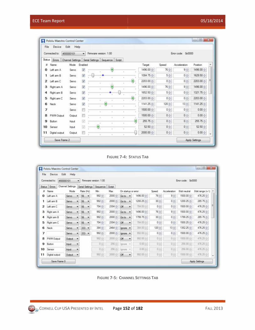
ECE Team Report 05/18/2014
CORNELL CUP USA PRESENTED BY INTEL Page 152 of 182 FALL 2013
FIGURE 7-4: STATUS TAB
FIGURE 7-5: CHANNEL SETTINGS TAB
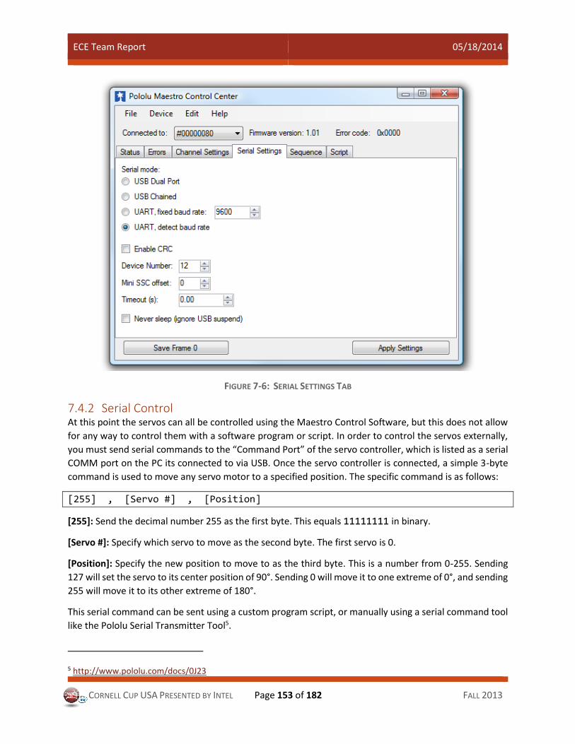
ECE Team Report 05/18/2014
CORNELL CUP USA PRESENTED BY INTEL Page 153 of 182 FALL 2013
FIGURE 7-6: SERIAL SETTINGS TAB
7.4.2 Serial Control At this point the servos can all be controlled using the Maestro Control Software, but this does not allow
for any way to control them with a software program or script. In order to control the servos externally,
you must send serial commands to the “Command Port” of the servo controller, which is listed as a serial
COMM port on the PC its connected to via USB. Once the servo controller is connected, a simple 3-byte
command is used to move any servo motor to a specified position. The specific command is as follows:
[255] , [Servo #] , [Position]
[255]: Send the decimal number 255 as the first byte. This equals 11111111 in binary.
[Servo #]: Specify which servo to move as the second byte. The first servo is 0.
[Position]: Specify the new position to move to as the third byte. This is a number from 0-255. Sending
127 will set the servo to its center position of 90°. Sending 0 will move it to one extreme of 0°, and sending
255 will move it to its other extreme of 180°.
This serial command can be sent using a custom program script, or manually using a serial command tool
like the Pololu Serial Transmitter Tool5.
5 http://www.pololu.com/docs/0J23
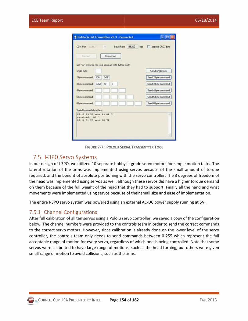
ECE Team Report 05/18/2014
CORNELL CUP USA PRESENTED BY INTEL Page 154 of 182 FALL 2013
FIGURE 7-7: POLOLU SERIAL TRANSMITTER TOOL
I-3P0 Servo Systems In our design of I-3PO, we utilized 10 separate hobbyist grade servo motors for simple motion tasks. The
lateral rotation of the arms was implemented using servos because of the small amount of torque
required, and the benefit of absolute positioning with the servo controller. The 3 degrees of freedom of
the head was implemented using servos as well, although these servos did have a higher torque demand
on them because of the full weight of the head that they had to support. Finally all the hand and wrist
movements were implemented using servos because of their small size and ease of implementation.
The entire I-3PO servo system was powered using an external AC-DC power supply running at 5V.
7.5.1 Channel Configurations After full calibration of all ten servos using a Pololu servo controller, we saved a copy of the configuration
below. The channel numbers were provided to the controls team in order to send the correct commands
to the correct servo motors. However, since calibration is already done on the lower level of the servo
controller, the controls team only needs to send commands between 0-255 which represent the full
acceptable range of motion for every servo, regardless of which one is being controlled. Note that some
servos were calibrated to have large range of motions, such as the head turning, but others were given
small range of motion to avoid collisions, such as the arms.

ECE Team Report 05/18/2014
CORNELL CUP USA PRESENTED BY INTEL Page 155 of 182 FALL 2013
FIGURE 8: I-3P0 SERVO CONFIGURATION
7.5.2 Pololu Controller Noise The only problem we encountered when using the Pololu servo controller was a reset scenario which
occurred when electrical noise spikes entered the system. This usually was due to plugging in the motor
controller bank, or running a higher power motor. Any large power draws like that caused the servo
controller to reset and lose connection with our controls team. To counter this situation, we found several
practices which we recommend using with the Pololu servo controllers.
1. Set every servo to return to its center (or default) position when powered on or after an error. This
can be done under the “Channel Settings” tab in the Maestro Control Center. It ensures that the servos
are always being sent a control signal when they are powered on, and it avoids the situation when
they are first powered on but receiving no control signal, leaving them completely susceptible to any
electrical noise on their signal lines. This noise can be interpreted as a control signal if the line is left
floating, and the servo could start moving completely out of its own range of motion, possibly breaking
itself or the system.
2. Do not power the Pololu servo controller using USB on the final system configuration. Instead, connect
the controller to a computer or microcontroller using the TTL logic ports. Connect TX, RX, and GND. A
USB-TTL adapter can be used to interface with a computer directly. Then power the controller with
the external 5V power supply which is running the servos, by putting on the supplied header jumper
as documented in the Pololu manual.
3. Add a 0.1𝜇𝐹 ceramic capacitor and a reasonably large electrolytic capacitor (100𝜇𝐹 or more) in
parallel with the 5V power inputs of the servo controller. This helps to dampen the noise on the power
lines as the servos pulse to move and hold their target positions.
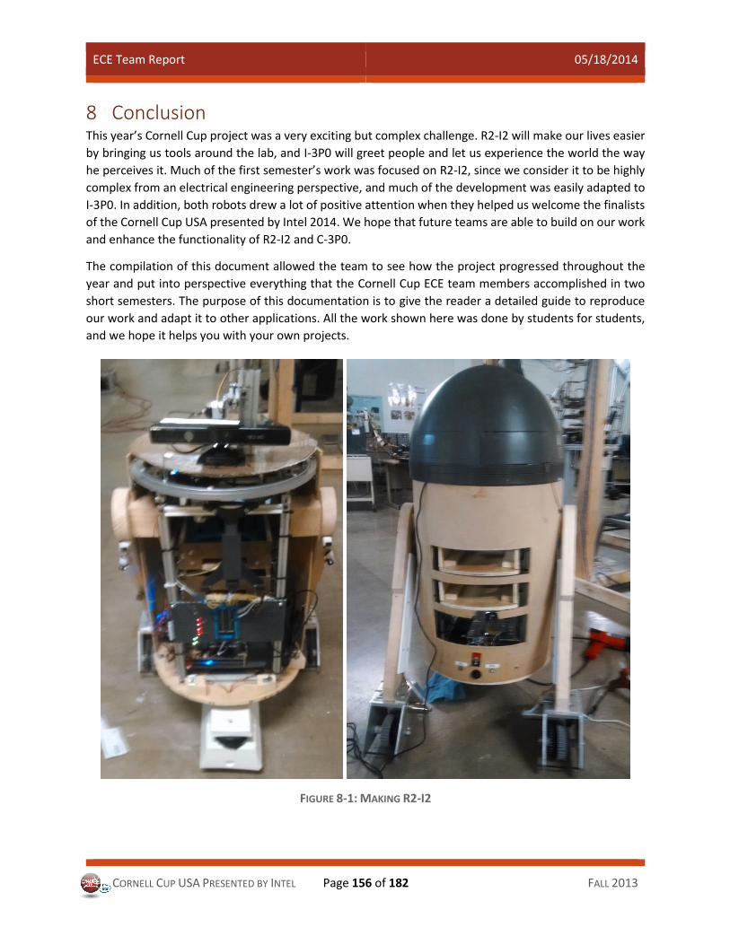
ECE Team Report 05/18/2014
CORNELL CUP USA PRESENTED BY INTEL Page 156 of 182 FALL 2013
8 Conclusion This year’s Cornell Cup project was a very exciting but complex challenge. R2-I2 will make our lives easier
by bringing us tools around the lab, and I-3P0 will greet people and let us experience the world the way
he perceives it. Much of the first semester’s work was focused on R2-I2, since we consider it to be highly
complex from an electrical engineering perspective, and much of the development was easily adapted to
I-3P0. In addition, both robots drew a lot of positive attention when they helped us welcome the finalists
of the Cornell Cup USA presented by Intel 2014. We hope that future teams are able to build on our work
and enhance the functionality of R2-I2 and C-3P0.
The compilation of this document allowed the team to see how the project progressed throughout the
year and put into perspective everything that the Cornell Cup ECE team members accomplished in two
short semesters. The purpose of this documentation is to give the reader a detailed guide to reproduce
our work and adapt it to other applications. All the work shown here was done by students for students,
and we hope it helps you with your own projects.
FIGURE 8-1: MAKING R2-I2
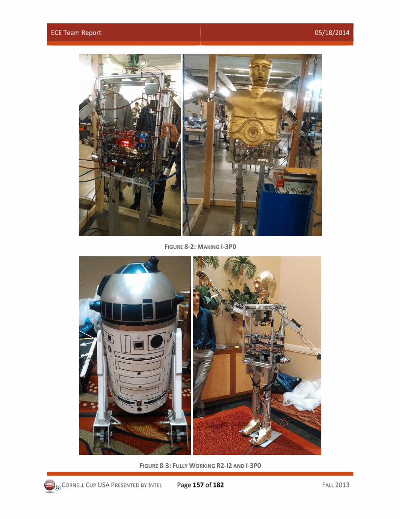
ECE Team Report 05/18/2014
CORNELL CUP USA PRESENTED BY INTEL Page 157 of 182 FALL 2013
FIGURE 8-2: MAKING I-3P0
FIGURE 8-3: FULLY WORKING R2-I2 AND I-3P0

ECE Team Report 05/18/2014
CORNELL CUP USA PRESENTED BY INTEL Page 158 of 182 FALL 2013
Appendix A – Acronym List Acronym Definition
AC Alternating Current
CD Compact Disc
CS Computer Science
DC Direct Current
DMM Digital Multi-Meter
DVD Digital Video Disc
ECE Electrical and Computer Engineering
EMF Electromagnetic Field
FPGA Field Programmable Gate Array
GPIO General Purpose Input/Output
GPS Global Positioning System
HDL Hardware Description Language
I/O Input/Output
IMU Inertial Measurement Unit
ISM Industrial, Scientific and Medical (radio bands)
ISO International Organization for Standardization
LCD Liquid Crystal Display
LED Light Emitting Diode
LIDAR Light Detection and Ranging (Portmanteau of Light and RADAR)
MOV Metal-Oxide Varistor
MOSFET Metal Oxide Semiconductor Field-Effect Transistor
NTC Negative Temperature Coefficient
PC Personal Computer
PCI Peripheral Component Interconnect
PCIe Peripheral Component Interconnect Express
PLL Phase-Locked Loop
PWM Pulse Width Modulation
RC Resistor Capacitor
RCD Resistor Capacitor Diode
RFID Radio Frequency Identification
SLAM Simultaneous Localization and Mapping
TTL Transistor-Transistor Logic
URL Uniform Resource Locator
USB Universal Serial Bus
TABLE A-1: ACRONYM LIST
Appendix B: I-3P0 walking code This section contains complete code listing including all functions used for testing (not necessarily used in
execution but required for testing and debugging). Multiple versions of the “main” code/function are
attached at the end.

ECE Team Report 05/18/2014
CORNELL CUP USA PRESENTED BY INTEL Page 159 of 182 FALL 2013
Buzzer.ino:
void InitBuzzer(){
TCCR1A = 0x82;
/* COM1A[1:0] = 10
- Clear on compare match
* COM1B = 0, COM1C = 0
- Normal port operation
* WGM1[1:0] = 10
- For fast PWM
*/
TCCR1B = 0x18;
/* WGM1[3:2] = 11
- For fast PWM
*/
TCCR1C = 0;
// Not using force outputs
ICR1H = 0x03; ICR1L = 0x1F;
OCR1AH = 0x01; OCR1AL = 0x90;
/* Configured for mode: fast PWM
* TOP = 800 = 0x031F;
* Want prescaler = 1:8
* That will give 2500Hz frequency (resonant freq of buzzer)
* Duty cycle = 50%
* Thus, period register = 400 = 0x0190
*
*
* I am using Timer 1 channel A
* That pin is RB5 which is 11 on the Mega 2560 board
*/
pinMode(11, OUTPUT);
}
void BuzzerOn(){
TCCR1B = 0x1A;
// Prescaler 1:8 to output 2509Hz for buzzer
}
void BuzzerOff(){
TCCR1B = 0x18;
// Clock off for Timer 1 - so buzzer off
}
void Beep(void){
unsigned char buzzerCount;
for (buzzerCount = 0; buzzerCount < 4; buzzerCount++){
BuzzerOn();
delay(200);
BuzzerOff();
delay(200);
}
}

ECE Team Report 05/18/2014
CORNELL CUP USA PRESENTED BY INTEL Page 160 of 182 FALL 2013
Generate_tables.ino:
//#define MaxSpeed 2200 // 1 second
//#define MaxSpeed 4901 // 0.67 seconds
//#define MaxSpeed 3000 // 0.856 seconds
#define MaxSpeed 3333 //0.66 seconds
//#define MaxSpeed 2774 //0.793 seconds
void GenerateSpeedTable(void){
unsigned char speedTableCounter;
unsigned char speedTableCountDown;
unsigned long neededSpeed;
for (speedTableCounter = 0; speedTableCounter < 16; speedTableCounter++){
neededSpeed = ((unsigned long)(speedTableCounter + 1) * MaxSpeed) >> 4;
if (neededSpeed < 7) neededSpeed = 7;
SpeedArray[speedTableCounter] = neededSpeed;
}
/*
SpeedArray[0] = SpeedArray[3];
SpeedArray[1] = SpeedArray[3];
SpeedArray[2] = SpeedArray[3];
*/
speedTableCountDown = 15;
for (speedTableCounter = 16; speedTableCounter < 32; speedTableCounter++){
neededSpeed = SpeedArray[speedTableCountDown];
if (neededSpeed < 7) neededSpeed = 7;
SpeedArray[speedTableCounter] = neededSpeed;
speedTableCountDown--;
}
/*
SpeedArray[0] = (SpeedArray[0] + SpeedArray[1]) >> 1;
SpeedArray[31] = SpeedArray[0];
SpeedArray[1] = (SpeedArray[1] + SpeedArray[2]) >> 1;
SpeedArray[30] = SpeedArray[1];
SpeedArray[2] = (SpeedArray[2] + SpeedArray[3]) >> 1;
SpeedArray[29] = SpeedArray[2];
*/
}

ECE Team Report 05/18/2014
CORNELL CUP USA PRESENTED BY INTEL Page 161 of 182 FALL 2013
Timer3.ino:
void configureTimer3(void){
// Need fast PWM, TOP = OCR3A
// Mode = 15: WGM[3:0] = 1111
// Timer 3 setup:
TCCR3A = 3;
Timer3_OFF;
TCCR3C = 0;
OCR3AH = 0x05; OCR3AL = 0x08; // 20.624ms
//OCR3AH = 0x05; OCR3AL = 0x1C; // 20.944ms
//OCR3AH = 0x06; OCR3AL = 0x87; // 26.75 ms
//OCR3AH = 0x06; OCR3AL = 0x0B; // 24.77 ms
//OCR3AH = 0x07; OCR3AL = 0xA0; // 31.25ms period
//OCR3AH = 0x0F; OCR3AL = 42; // 62.5ms period
//OCR3AH= 0x18; OCR3AL = 0x69; // 100ms period
//OCR3AH = 0x49; OCR3AL = 0x3D; // 300ms period
TIMSK3 = 2; // Turn on Timer 3 compare match A interrupt
sei(); // Turn on interrupts
}
ISR(TIMER3_COMPA_vect){
if (flgUpdate){
timeInterval++;
if (timeInterval == 32){
timeInterval = 0;
Timer3_OFF;
flgUpdate = 0;
}
}
}

ECE Team Report 05/18/2014
CORNELL CUP USA PRESENTED BY INTEL Page 162 of 182 FALL 2013
getCommand.ino:
char getCommand(void){
unsigned char stepCount;
if (Serial.available()){
byte1 = Serial.read(); // Get unlock code
if (byte1 == UNLOCK_CODE){
byte2 = Serial.read(); // Get tens of no. of steps
if (byte2 == '1'){ // 2 digit number
byte3 = Serial.read(); // Get ones of no. of steps
}
else{
byte3 = Serial.read();
if ((byte3 == 13) || (byte3 == 10)){
byte3 = byte2; // One digit only
byte2 = '0';
}
}
}
if ((byte2 >= '0') && (byte2 <= '9') && (byte3 >= '0') && (byte3 <= '9')){
byte2 = byte2 - '0'; byte3 = byte3 - '0';
stepCount = byte2 * 10 + byte3;
if(stepCount <= MAX_STEPS){
if (((stepCount >> 1) << 1) == stepCount){ // Even number
return stepCount;
}
else return (-1); // odd number
}
else return (-2); // out of bounds
}
else return (-4); // invalid input
}
else return (-5); // no connection
}

ECE Team Report 05/18/2014
CORNELL CUP USA PRESENTED BY INTEL Page 163 of 182 FALL 2013
getP:
int getPosition(unsigned char channel){
unsigned char signReceived; // 1 = negative, 0 = positive
long currentPosition;
signReceived = 0;
index = 0;
unsigned char positions;
char index2 = 0;
if (channel == 1){
BUFFER[0] = '1';
}
else{
BUFFER[0] = '2';
}
BUFFER[1] = ',';
BUFFER[2] = 'g';
BUFFER[3] = 'e';
BUFFER[4] = 't';
BUFFER[5] = 'p';
sendKangaroo(6); NEWLINE_KANGAROO;
delay(120);
while (Kangaroo.available()){
positions = Kangaroo.read();
#define LFp (positions == 10)
#define CRp (positions == 13)
#define COMMAp (positions == ',')
#define RANGE1p ((positions >= '0') && (positions <= '9'))
#define RANGE2p ((positions >= 'a') && (positions <= 'z'))
#define RANGE3p ((positions >= 'A') && (positions <= 'Z'))
if (RANGE1p | RANGE2p | RANGE3p | COMMAp)
{
pArray[index] = positions;
index++;
//Serial.print(positions);
}
if (positions == '-') signReceived = 1; // negative
}
unsigned char i;
//Serial.println(index);
// index now holds index value of new line, ie the length of received data
in pArray
// Received data should be in format "1,Pxxxx" where x is position and is
not of fixed length

ECE Team Report 05/18/2014
CORNELL CUP USA PRESENTED BY INTEL Page 164 of 182 FALL 2013
switch (index){
case 4: // 1 digit
dig1 = pArray[3];
currentPosition = dig1 - 48; //atoi(dig1);
break;
case 5: // 2 digit
dig2[0] = pArray[3];
dig2[1] = pArray[4];
currentPosition = (dig2[0] - 48) * 10 + (dig2[1] - 48);
//currentPosition = atoi(dig2);
break;
case 6: // 3 digit
dig3[0] = pArray[3];
dig3[1] = pArray[4];
dig3[2] = pArray[5];
currentPosition = (dig3[0] - 48) * 100 + (dig3[1] - 48) * 10 +
(dig3[2] - 48);
//currentPosition = atoi(dig3);
break;
case 7: // 4 digit
dig4[0] = pArray[3];
dig4[1] = pArray[4];
dig4[2] = pArray[5];
dig4[3] = pArray[6];
currentPosition = (dig4[0] - 48) * 1000 + (dig4[1] - 48) * 100 +
(dig4[2] - 48) * 10 + (dig4[3] - 48);
//currentPosition = atoi(dig4);
break;
case 8: // 5 digit
dig5[0] = pArray[3];
dig5[1] = pArray[4];
dig5[2] = pArray[5];
dig5[3] = pArray[6];
dig5[4] = pArray[7];
currentPosition = (dig5[0] - 48) * 10000 + (dig5[1] - 48) * 1000 +
(dig5[2] - 48) * 100 + (dig5[3] - 48) * 10 + (dig5[4] - 48);
//currentPosition = atoi(dig5);
break;
}
if (index > 8){
currentPosition = 0;
}
if (signReceived == 1) currentPosition = currentPosition * (-1);
return currentPosition;
}
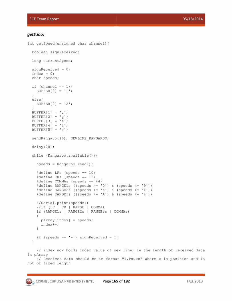
ECE Team Report 05/18/2014
CORNELL CUP USA PRESENTED BY INTEL Page 165 of 182 FALL 2013
getS.ino:
int getSpeed(unsigned char channel){
boolean signReceived;
long currentSpeed;
signReceived = 0;
index = 0;
char speeds;
if (channel == 1){
BUFFER[0] = '1';
}
else{
BUFFER[0] = '2';
}
BUFFER[1] = ',';
BUFFER[2] = 'g';
BUFFER[3] = 'e';
BUFFER[4] = 't';
BUFFER[5] = 's';
sendKangaroo(6); NEWLINE_KANGAROO;
delay(20);
while (Kangaroo.available()){
speeds = Kangaroo.read();
#define LFs (speeds == 10)
#define CRs (speeds == 13)
#define COMMAs (speeds == 44)
#define RANGE1s ((speeds >= '0') & (speeds <= '9'))
#define RANGE2s ((speeds >= 'a') & (speeds <= 'z'))
#define RANGE3s ((speeds >= 'A') & (speeds <= 'Z'))
//Serial.print(speeds);
//if (LF | CR | RANGE | COMMA)
if (RANGE1s | RANGE2s | RANGE3s | COMMAs)
{
pArray[index] = speeds;
index++;
}
if (speeds == '-') signReceived = 1;
}
// index now holds index value of new line, ie the length of received data
in pArray
// Received data should be in format "1,Pxxxx" where x is position and is
not of fixed length

ECE Team Report 05/18/2014
CORNELL CUP USA PRESENTED BY INTEL Page 166 of 182 FALL 2013
switch (index){
case 4: // 1 digit
dig1 = pArray[3];
currentSpeed = dig1 - 48; //atoi(dig1);
break;
case 5: // 2 digit
dig2[0] = pArray[3];
dig2[1] = pArray[4];
currentSpeed = (dig2[0] - 48) * 10 + (dig2[1] - 48);
//currentPosition = atoi(dig2);
break;
case 6: // 3 digit
dig3[0] = pArray[3];
dig3[1] = pArray[4];
dig3[2] = pArray[5];
currentSpeed = (dig3[0] - 48) * 100 + (dig3[1] - 48) * 10 + (dig3[2]
- 48);
//currentPosition = atoi(dig3);
break;
case 7: // 4 digit
dig4[0] = pArray[3];
dig4[1] = pArray[4];
dig4[2] = pArray[5];
dig4[3] = pArray[6];
currentSpeed = (dig4[0] - 48) * 1000 + (dig4[1] - 48) * 100 +
(dig4[2] - 48) * 10 + (dig4[3] - 48);
//currentPosition = atoi(dig4);
break;
case 8: // 5 digit
dig5[0] = pArray[3];
dig5[1] = pArray[4];
dig5[2] = pArray[5];
dig5[3] = pArray[6];
dig5[4] = pArray[7];
currentSpeed = (dig5[0] - 48) * 10000 + (dig5[1] - 48) * 1000 +
(dig5[2] - 48) * 100 + (dig5[3] - 48) * 10 + (dig5[4] - 48);
//currentPosition = atoi(dig5);
break;
}
//Serial.println(currentPosition);
if (index > 8){
currentSpeed = 0;
}
if (signReceived == 1) currentSpeed = currentSpeed * (-1);
return currentSpeed;
}

ECE Team Report 05/18/2014
CORNELL CUP USA PRESENTED BY INTEL Page 167 of 182 FALL 2013
rampTimed.ino: // directions = 1 --> move in positive direction
// directions = 0 --> move in negative direction
void rampTimed(unsigned char channel, boolean directions){
if (channel == 1) channel = 1; else channel = 2;
TCNT3H = 0; TCNT3L = 0;
flgUpdate = 1; Timer3_ON;
while (flgUpdate == 1){
if (directions) sendSpeed(channel, SpeedArray[timeInterval]);
else sendSpeed(channel, (-1) * SpeedArray[timeInterval]);
}
sendSpeed(channel,0);
}
void rampTimed_n(unsigned char channel, boolean directions, unsigned char num){
unsigned char rampCounter;
unsigned char oldSpeed;
unsigned char maxSpeed;
/*if (num > 1){
oldSpeed = SpeedArray[0];
maxSpeed = SpeedArray[15];
}*/
if (channel == 1) channel = 1; else channel = 2;
TCNT3H = 0; TCNT3L = 0;
flgUpdate = 1; Timer3_ON;
for (rampCounter = 0; rampCounter < num; rampCounter++){
flgUpdate = 1; Timer3_ON;
while (flgUpdate == 1){
if (directions) sendSpeed(channel, SpeedArray[timeInterval]);
else sendSpeed(channel, (-1) * SpeedArray[timeInterval]);
}
// SpeedArray[0] = maxSpeed;
directions = !directions;
}
// SpeedArray[0] = oldSpeed;
sendSpeed(channel, 0); // Stop motor
// Timer3_OFF;
}

ECE Team Report 05/18/2014
CORNELL CUP USA PRESENTED BY INTEL Page 168 of 182 FALL 2013
sendP.ino:
void sendPosition(unsigned char channel, int positions){
unsigned char len;
if (channel == 1) channel = 1;
else channel = 2;
BUFFER[0] = channel + '0';
BUFFER[1] = ',';
BUFFER[2] = 'p';
if (positions < 0) BUFFER[3] = '-'; else BUFFER[3] = ' ';
positions = abs(positions);
if (positions < 10){
len = 5;
BUFFER[4] = positions + '0';
}
else if (positions < 100){
len = 6;
BUFFER[4] = positions/10 + '0';
BUFFER[5] = positions % 10 + '0';
}
else if (positions < 1000){
len = 7;
BUFFER[4] = positions/100 + '0';
BUFFER[5] = ((positions/10) % 10) + '0';
BUFFER[6] = (positions % 10) + '0';
}
else{
len = 8;
BUFFER[4] = positions/1000 + '0';
BUFFER[5] = ((positions/100) % 10) + '0';
BUFFER[6] = ((positions/10) % 10) + '0';
BUFFER[7] = (positions % 10) + '0';
}
sendKangaroo(len); NEWLINE_KANGAROO;
}

ECE Team Report 05/18/2014
CORNELL CUP USA PRESENTED BY INTEL Page 169 of 182 FALL 2013
sendSpeed.ino:
void sendSpeed(unsigned char channel, int speeds){
unsigned char len;
if (channel == 1) channel = 1;
else channel = 2;
BUFFER[0] = channel + '0';
BUFFER[1] = ',';
BUFFER[2] = 's';
if (speeds < 0) BUFFER[3] = '-'; else BUFFER[3] = ' ';
speeds = abs(speeds);
if (speeds < 10){
len = 5;
BUFFER[4] = speeds + '0';
}
else if (speeds < 100){
len = 6;
BUFFER[4] = speeds/10 + '0';
BUFFER[5] = speeds % 10 + '0';
}
else if (speeds < 1000){
len = 7;
BUFFER[4] = speeds/100 + '0';
BUFFER[5] = ((speeds/10) % 10) + '0';
BUFFER[6] = (speeds % 10) + '0';
}
else{
len = 8;
BUFFER[4] = speeds/1000 + '0';
BUFFER[5] = ((speeds/100) % 10) + '0';
BUFFER[6] = ((speeds/10) % 10) + '0';
BUFFER[7] = (speeds % 10) + '0';
}
sendKangaroo(len); NEWLINE_KANGAROO;
}

ECE Team Report 05/18/2014
CORNELL CUP USA PRESENTED BY INTEL Page 170 of 182 FALL 2013
walkSequence.ino:
void walkSequence(unsigned char steps){
Beep();
InitMC(TORSO);
InitMC(LEG);
delay(7000);
UNBRAKE;
sendPosition(TORSO, -550);
delay(500);
walk(steps);
delay(2000);
BRAKE;
}
ECE Team Report 05/18/2014
CORNELL CUP USA PRESENTED BY INTEL Page 171 of 182 FALL 2013
walkTest.ino:
void walk_left(unsigned int steps){
unsigned int walkCounter;
boolean directions;
unsigned int steps_buffer;
unsigned int sbuffer;
unsigned int oldTime;
boolean flgSent;
unsigned char bufferCounter;
unsigned int Pcurrent;
BUFFER_WALK[0] = '1';
BUFFER_WALK[1] = ',';
BUFFER_WALK[2] = 'p';
BUFFER_WALK[3] = ' ';
BUFFER_WALK[4] = ' ';
BUFFER_WALK[5] = ' ';
BUFFER_WALK[6] = ' ';
BUFFER_WALK[7] = ' ';
BUFFER_WALK[8] = ' ';
BUFFER_WALK[9] = 's';
BUFFER_WALK[10] = ' ';
BUFFER_WALK[11] = '1';
BUFFER_WALK[12] = '5';
BUFFER_WALK[13] = '1';
//Beep();
InitMC(TORSO);
InitMC(LEG);
delay(7000);
//sendPosition(TORSO, 550);
Kangaroo.println("2, p550 s550");
delay(3000);
steps_buffer = steps * 100;
sbuffer = (steps_buffer/1000) + '0';
if (steps >= 10) BUFFER_WALK[4] = sbuffer;
sbuffer = ((steps_buffer/100) % 10) + '0';
BUFFER_WALK[5] = sbuffer;
sbuffer = ((steps_buffer/10) % 10) + '0';
BUFFER_WALK[6] = sbuffer;
sbuffer = (steps_buffer % 10) + '0';
BUFFER_WALK[7] = sbuffer;
TCNT3H = 0; TCNT3L = 0; flgUpdate = 1; Timer3_ON;
oldTime = 0;
flgSent = 0;
directions = 0;
ECE Team Report 05/18/2014
CORNELL CUP USA PRESENTED BY INTEL Page 172 of 182 FALL 2013
for (walkCounter = 0; walkCounter < (steps + 1); walkCounter++){
flgUpdate = 1; Timer3_ON;
while (flgUpdate == 1){
if ((timeInterval == 15) && (flgSent == 0)){ // Send walking command if
not already sent
for (bufferCounter = 0; bufferCounter < 14; bufferCounter++){
SENDKANGAROO(BUFFER_WALK[bufferCounter]);
}
NEWLINE_KANGAROO;
flgSent = 1;
}
if (directions) sendSpeed(TORSO, SpeedArray[timeInterval]);
else sendSpeed(TORSO, (-1) * SpeedArray[timeInterval]);
}
directions = !directions;
}
sendSpeed(TORSO, 0);
}
void walk_right(unsigned int steps){
unsigned int walkCounter;
boolean directions;
unsigned int steps_buffer;
unsigned int sbuffer;
unsigned int oldTime;
boolean flgSent;
unsigned char bufferCounter;
unsigned int Pcurrent;
BUFFER_WALK[0] = '1';
BUFFER_WALK[1] = ',';
BUFFER_WALK[2] = 'p';
BUFFER_WALK[3] = ' ';
BUFFER_WALK[4] = ' ';
BUFFER_WALK[5] = ' ';
BUFFER_WALK[6] = ' ';
BUFFER_WALK[7] = ' ';
BUFFER_WALK[8] = ' ';
BUFFER_WALK[9] = 's';
BUFFER_WALK[10] = ' ';
BUFFER_WALK[11] = '1';
BUFFER_WALK[12] = '5';
BUFFER_WALK[13] = '1';
//Beep();
InitMC(TORSO); InitMC(LEG);
delay(7000);
/*
Pcurrent = getPosition(TORSO);
while (Pcurrent > -560){
Pcurrent = getPosition(TORSO);
}
*/
sendPosition(TORSO, -550);

ECE Team Report 05/18/2014
CORNELL CUP USA PRESENTED BY INTEL Page 173 of 182 FALL 2013
delay(2000);
steps_buffer = steps * 100;
sbuffer = (steps_buffer/1000) + '0';
if (steps >= 10) BUFFER_WALK[4] = sbuffer;
sbuffer = ((steps_buffer/100) % 10) + '0';
BUFFER_WALK[5] = sbuffer;
sbuffer = ((steps_buffer/10) % 10) + '0';
BUFFER_WALK[6] = sbuffer;
sbuffer = (steps_buffer % 10) + '0';
BUFFER_WALK[7] = sbuffer;
TCNT3H = 0; TCNT3L = 0; flgUpdate = 1; Timer3_ON;
oldTime = 0;
flgSent = 0;
directions = 1;
for (walkCounter = 0; walkCounter < (steps + 1); walkCounter++){
flgUpdate = 1; Timer3_ON;
while (flgUpdate == 1){
if ((timeInterval == 15) && (flgSent == 0)){ // Send walking command if
not already sent
for (bufferCounter = 0; bufferCounter < 14; bufferCounter++){
SENDKANGAROO(BUFFER_WALK[bufferCounter]);
}
NEWLINE_KANGAROO;
flgSent = 1;
}
if (directions) sendSpeed(TORSO, SpeedArray[timeInterval]);
else sendSpeed(TORSO, (-1) * SpeedArray[timeInterval]);
}
directions = !directions;
}
sendSpeed(TORSO, 0);
}
void walk(unsigned int steps){
unsigned int walkCounter;
boolean directions;
unsigned int steps_buffer;
unsigned int sbuffer;
unsigned int oldTime;
boolean flgSent;
unsigned char bufferCounter;
BUFFER_WALK[0] = '1';
BUFFER_WALK[1] = ',';
BUFFER_WALK[2] = 'p';
BUFFER_WALK[3] = ' ';
ECE Team Report 05/18/2014
CORNELL CUP USA PRESENTED BY INTEL Page 174 of 182 FALL 2013
BUFFER_WALK[4] = ' ';
BUFFER_WALK[5] = ' ';
BUFFER_WALK[6] = ' ';
BUFFER_WALK[7] = ' ';
BUFFER_WALK[8] = ' ';
BUFFER_WALK[9] = 's';
BUFFER_WALK[10] = ' ';
BUFFER_WALK[11] = '1';
BUFFER_WALK[12] = '5';
BUFFER_WALK[13] = '1';
//Beep();
steps_buffer = steps * 100;
sbuffer = (steps_buffer/1000) + '0';
if (steps >= 10) BUFFER_WALK[4] = sbuffer;
sbuffer = ((steps_buffer/100) % 10) + '0';
BUFFER_WALK[5] = sbuffer;
sbuffer = ((steps_buffer/10) % 10) + '0';
BUFFER_WALK[6] = sbuffer;
sbuffer = (steps_buffer % 10) + '0';
BUFFER_WALK[7] = sbuffer;
TCNT3H = 0; TCNT3L = 0; flgUpdate = 1; Timer3_ON;
oldTime = 0;
flgSent = 0;
directions = 1;
for (walkCounter = 0; walkCounter < (steps+1); walkCounter++){
flgUpdate = 1; Timer3_ON;
while (flgUpdate == 1){
if ((timeInterval == 15) && (flgSent == 0)){ // Send walking command if
not already sent
for (bufferCounter = 0; bufferCounter < 14; bufferCounter++){
SENDKANGAROO(BUFFER_WALK[bufferCounter]);
}
NEWLINE_KANGAROO;
flgSent = 1;
}
if (directions) sendSpeed(TORSO, SpeedArray[timeInterval]);
else sendSpeed(TORSO, (-1) * SpeedArray[timeInterval]);
}
directions = !directions;
}
sendSpeed(TORSO, 0);
}
void walk_one(void){
Beep();
walk_right(1);

ECE Team Report 05/18/2014
CORNELL CUP USA PRESENTED BY INTEL Page 175 of 182 FALL 2013
//delay(1000);
Beep();
walk_left(1);
sendSpeed(LEG, 0);
delay(1000);
//Kangaroo.println("2, p-550 s550");
}
ECE Team Report 05/18/2014
CORNELL CUP USA PRESENTED BY INTEL Page 176 of 182 FALL 2013
Main versions:
arduinomotcon.ino: (taking steps in 2’s) #define Kangaroo Serial2
#define TORSO 2
#define LEG 1
#define Timer3_ON {TCCR3B = 0x1C;} // Prescaler: 1/256
#define Timer3_OFF {TCCR3B = 0x18;} // Timer off
#define BrakePin 7
#define UNBRAKE {digitalWrite(BrakePin, HIGH);}
#define BRAKE {digitalWrite(BrakePin, LOW);}
#define UNLOCK_CODE 'j'
#define MAX_STEPS 12
char retVal;
unsigned int dummyINT;
volatile unsigned int timeInterval;
volatile boolean flgUpdate;
volatile char BUFFER[10];
char pArray[16];
unsigned char byte1; // First byte obtained from computer command -> unlock
code
unsigned char byte2; // Second byte obtained from computer command -> tens of
no. of steps
unsigned char byte3; // Third byte obtained from computer command -> units of
no. of steps
unsigned char index;
unsigned char errorCode;
boolean flgError;
unsigned char numberOfSteps;
unsigned int SpeedArray[32];
char BUFFER_WALK[14];
char dig1; // Buffer to store 1 digit value of position
char dig2[2]; // Buffer to store 2 digit value of position
char dig3[3]; // Buffer to store 3 digit value of position
char dig4[4]; // Buffer to store 4 digit value of position
char dig5[5]; // Buffer to store 5 digit value of position
char dig6[6]; // Buffer to store 6 digit value of position
ECE Team Report 05/18/2014
CORNELL CUP USA PRESENTED BY INTEL Page 177 of 182 FALL 2013
unsigned long cPosition[16];
unsigned int sRamp[16];
#define SEND Serial.write
#define SENDKANGAROO Kangaroo.write
#define NEWLINE {SEND(13); SEND(10);}
#define NEWLINE_KANGAROO {SENDKANGAROO(13); SENDKANGAROO(10);}
void sendSerial(unsigned char n){
unsigned char serialCounter;
for (serialCounter=0; serialCounter < n; serialCounter++){
SEND(BUFFER[serialCounter]);
}
}
void sendKangaroo(unsigned char n){
unsigned char serialCounter;
for (serialCounter=0; serialCounter < n; serialCounter++){
SENDKANGAROO(BUFFER[serialCounter]);
//Serial.print(BUFFER[serialCounter]);
}
//NEWLINE;
}
void del(void){
delay(1000);
}
void InitMC(unsigned char channel){
if (channel == 1) channel = 1;
else channel = 2;
BUFFER[0] = channel + '0';
BUFFER[1] = ',';
BUFFER[2] = 's';
BUFFER[3] = 't';
BUFFER[4] = 'a';
BUFFER[5] = 'r';
BUFFER[6] = 't';
sendKangaroo(7); NEWLINE_KANGAROO;
BUFFER[2] = 'h';
BUFFER[3] = 'o';
BUFFER[4] = 'm';
BUFFER[5] = 'e';
sendKangaroo(6); NEWLINE_KANGAROO;
delay(100);
}
void sendHome(unsigned char channel){

ECE Team Report 05/18/2014
CORNELL CUP USA PRESENTED BY INTEL Page 178 of 182 FALL 2013
if (channel == 1) channel = 1;
else channel = 2;
BUFFER[0] = channel + '0';
BUFFER[1] = ',';
BUFFER[2] = 'h';
BUFFER[3] = 'o';
BUFFER[4] = 'm';
BUFFER[5] = 'e';
sendKangaroo(6); NEWLINE_KANGAROO;
delay(20);
}
void setup() {
pinMode(BrakePin, OUTPUT);
Serial.begin(9600);
Kangaroo.begin(115200);
//InitMC(TORSO);
//InitMC(LEG);
configureTimer3();
InitBuzzer();
BuzzerOff();
GenerateSpeedTable();
}
void dummyReads(){
unsigned int dummyVar;
dummyVar = getPosition(2); delay(100);
dummyVar = getSpeed(2); delay(100);
}
void loop() {
//Beep();
while (1){
retVal = getCommand();
if (retVal > 0){
numberOfSteps = retVal;
walkSequence(numberOfSteps);
}
else{
delay(500);
}
}
}
ECE Team Report 05/18/2014
CORNELL CUP USA PRESENTED BY INTEL Page 179 of 182 FALL 2013
arduinomotcon_disney.ino
#define Kangaroo Serial2
#define TORSO 2
#define LEG 1
#define Timer3_ON {TCCR3B = 0x1C;} // Prescaler: 1/256
#define Timer3_OFF {TCCR3B = 0x18;} // Timer off
#define BrakePin 7
#define UNBRAKE {digitalWrite(BrakePin, HIGH);}
#define BRAKE {digitalWrite(BrakePin, LOW);}
#define UNLOCK_CODE 'j'
#define MAX_STEPS 12
#define PC_IN_TWOS 0 // the original - controlled from Putty - take commands in
steps of 2
#define TEST_1_PLUS_1 1 // the test one - right leg pause left leg and that's
it
#define n_1_PLUS_1 2 // right leg pause left leg - repeat n times
#define Right_only 3 // only right leg - once
#define Left_only 4 // only left leg - once
#define MODE TEST_1_PLUS_1
unsigned char n_steps;
unsigned char n_counter;
char retVal;
unsigned int dummyINT;
volatile unsigned int timeInterval;
volatile boolean flgUpdate;
volatile char BUFFER[10];
char pArray[16];
unsigned char byte1; // First byte obtained from computer command -> unlock
code
unsigned char byte2; // Second byte obtained from computer command -> tens of
no. of steps
unsigned char byte3; // Third byte obtained from computer command -> units of
no. of steps
unsigned char index;
unsigned char errorCode;
boolean flgError;
unsigned char numberOfSteps;
unsigned int SpeedArray[32];

ECE Team Report 05/18/2014
CORNELL CUP USA PRESENTED BY INTEL Page 180 of 182 FALL 2013
char BUFFER_WALK[14];
char dig1; // Buffer to store 1 digit value of position
char dig2[2]; // Buffer to store 2 digit value of position
char dig3[3]; // Buffer to store 3 digit value of position
char dig4[4]; // Buffer to store 4 digit value of position
char dig5[5]; // Buffer to store 5 digit value of position
char dig6[6]; // Buffer to store 6 digit value of position
unsigned long cPosition[16];
unsigned int sRamp[16];
#define SEND Serial.write
#define SENDKANGAROO Kangaroo.write
#define NEWLINE {SEND(13); SEND(10);}
#define NEWLINE_KANGAROO {SENDKANGAROO(13); SENDKANGAROO(10);}
void sendSerial(unsigned char n){
unsigned char serialCounter;
for (serialCounter=0; serialCounter < n; serialCounter++){
SEND(BUFFER[serialCounter]);
}
}
void sendKangaroo(unsigned char n){
unsigned char serialCounter;
for (serialCounter=0; serialCounter < n; serialCounter++){
SENDKANGAROO(BUFFER[serialCounter]);
//Serial.print(BUFFER[serialCounter]);
}
//NEWLINE;
}
void del(void){
delay(1000);
}
void InitMC(unsigned char channel){
if (channel == 1) channel = 1;
else channel = 2;
BUFFER[0] = channel + '0';
BUFFER[1] = ',';
BUFFER[2] = 's';
BUFFER[3] = 't';
BUFFER[4] = 'a';
BUFFER[5] = 'r';
BUFFER[6] = 't';
sendKangaroo(7); NEWLINE_KANGAROO;
BUFFER[2] = 'h';
BUFFER[3] = 'o';

ECE Team Report 05/18/2014
CORNELL CUP USA PRESENTED BY INTEL Page 181 of 182 FALL 2013
BUFFER[4] = 'm';
BUFFER[5] = 'e';
sendKangaroo(6); NEWLINE_KANGAROO;
delay(100);
}
void sendHome(unsigned char channel){
if (channel == 1) channel = 1;
else channel = 2;
BUFFER[0] = channel + '0';
BUFFER[1] = ',';
BUFFER[2] = 'h';
BUFFER[3] = 'o';
BUFFER[4] = 'm';
BUFFER[5] = 'e';
sendKangaroo(6); NEWLINE_KANGAROO;
delay(20);
}
void setup() {
pinMode(BrakePin, OUTPUT);
BRAKE;
Serial.begin(9600);
Kangaroo.begin(115200);
//InitMC(TORSO);
//InitMC(LEG);
configureTimer3();
InitBuzzer();
BuzzerOff();
GenerateSpeedTable();
}
void dummyReads(){
unsigned int dummyVar;
dummyVar = getPosition(2); delay(100);
dummyVar = getSpeed(2); delay(100);
}
void loop() {
UNBRAKE;
walk_one();
//walk_one();
BRAKE;
while(1);

ECE Team Report 05/18/2014
CORNELL CUP USA PRESENTED BY INTEL Page 182 of 182 FALL 2013
n_steps = 2;
/*
InitMC(TORSO);
delay(5000);
sendPosition(TORSO, -550);
while(1);
*/
//while (1){
switch (MODE){
case PC_IN_TWOS: {
retVal = getCommand();
if (retVal > 0){
numberOfSteps = retVal;
walkSequence(numberOfSteps);
}
else{
delay(500);
}
break;
};
case TEST_1_PLUS_1: {
UNBRAKE;
//Beep();
walk_one();
BRAKE;
break;
};
case n_1_PLUS_1: {
UNBRAKE;
Beep();
for (n_counter = 0; n_counter < n_steps; n_counter++){
walk_one();
}
BRAKE;
break;
};
case Right_only: {
UNBRAKE;
Beep();
walk_right(1);
delay(2000);
BRAKE;
break;
};
case Left_only: {
UNBRAKE;
Beep();
walk_left(1);
delay(2000);
BRAKE;
break;
};
}
//}
while (1);
}