ece-311pages.cs.wisc.edu/~kzhao32/projects/ece311communication...ece 311 communication engineering...
TRANSCRIPT

ECE-311Experiment #1
Getting To Know the Laboratory’s Equipment
Objective:
In this exercise you will become familiar with the communication laboratory’s equipment, which will beused in the hardware experiments during this semester. The three main pieces of equipment are thefunction generator, the oscilloscope, and the spectrum analyzer. The other piece of equipment that you willuse is a power supply. The function generator and spectrum analyzer will be the main focus of yourinvestigations since it is assumed you are all expert oscilloscope users and power supply adjusters.
In addition, you will review and use your knowledge and skills in measuring and calculating the power of asignal.
Introduction:
Your laboratory teaching assistant will give you a brief lecture and demonstration on the use of the functiongenerator and spectrum analyzer.
Pre-Lab:
Calculate the theoretically expected average and RMS values for the waveforms of Part One in the “Task”section.
Calculate the theoretically expected powers for the sinusoids of Part Two in the “Task” section. Express
Task:
Part One:
Use the function generator to produce the following periodic waveforms:
Waveform FundamentalFrequency
Peak-to-PeakAmplitude
d.c. Offset
Square wave(Rectangular Wave with50% duty cycle)
1 MHz 3 volts 0 volts
Rectangular Wave with20% duty cycle
5 MHz 5 volts *
Triangular Wave 100 KHz 2 volts *Sawtooth Wave 100 KHz 3 volts 0 volts
*Adjust the d.c. offset so the “baseline “ of the signal is zero volts.
a) Display each waveform on the oscilloscope. First, show one period and then ten periods.b) Use the oscilloscope’s “soft” keys to measure the signal’s frequency, average value, and RMS
value. Record these values.c) Draw a sketch of each waveform. Label all critical points. (One period will be adequate.)

Part Two
1. Produce a 1 MHz sine wave with an amplitude of one (1) volt (2 volts peak-to-peak) and anaverage value of zero. Use the oscilloscope to verify the signal’s parameters.
2. Next, use the spectrum analyzer to measure the signal’s amplitude in dBmV and volts and itspower in dBm. Record these measurements
3. Repeat the previous two steps for sinusoids of amplitudes of two (2) and three (3) volts.4. Repeat the previous three steps for a sinusoid of 5 MHz.
Note that you will have taken data for six different sinusoids.
If you are having difficulty doing any of these measurements, ask for help from yourlaboratory teaching assistant.
Data Analysis:
For Part Two’s data, is there any relationship between the theoretically calculated and measured amplitudesand powers? There may not be any obvious correlation between the two because of either an unforeseensystematic error in taking the data or a mistake in the circuit model used to do the theoretical calculation.However, if you choose one signal as a reference signal (say the unit amplitude sinusoid) and take the ratioof the other signals’ amplitudes (or powers) to it. The expected and measured values of these ratios shouldbe very close. This illustrates a very important fact in communication systems; it is the relative signallevels that are important not absolute levels.
Report:
In your report for Part One include the sketches of the periodic waveforms you studied and a comparisonof the calculated and measured average and RMS values.
In your report for Part Two include a table (see below) comparing the expected and measured values forthe amplitudes and powers of the various sinusoids along with the ratios you calculated in the “dataanalysis” section.
Freq.(Hz)
ExpectedAmplitude(dBmV)
MeasuredAmplitude(dBmV)
CalculatedPower(dBm)
CalculatedRelative*Power (dB)
MeasuredPower(dBm)
MeasuredRelative*Power (dB)
*Use the unit amplitude sinusoid as the reference.
Prelative (dB) = P (dBm) – Preference (dBm)

============================================================================USEFUL INFORMATION
Decibel Formulae:
Amplitude (in dBm) = mW
P
1log10 Amplitude (in dBmV) =
mV
V
1log20
P is in Watts V is in Volts
Duty Cycle Defined:
Rectangular Pulse TrainPulse Width = tau
0
0.5
1
1.5
time
Period = To
! " #$ % "&'(o) X 100
Average Value and Power for a Periodic Signal:
Suppose, in the following, f(t) is a real, periodic signal with a fundamental period of T0. Then, the averagevalue of f(t) is
∫+
=⟩⟨0
)(1
)(0
Tt
t
x
x
dttfT
tf Volts (or Amps).
Next, the average power of f(t) is
∫+
=⟩⟨=0
)(1
)( 2
0
2Tt
t
ave
x
x
dttfT
tfP Watts.
In the above, tx is arbitrary indicating that the integrations are over the total period, but may “start”anywhere.
Finally, the RMS (root mean square) value of f(t) is just the square root of Pave. Note, that some times Pave
is referred to as the mean square value of f(t).
The average power formula given above assumes the signal is developed across a one-ohm resistor. Forother resistance values a modification must be made to the number calculated above. If f(t) is a voltage(current) the Pave must be divided (multiplied) by the actual resistance value to get the actual power in thesignal.

ECE 311 Communication Engineering
Lab Assignment #2
The Spectra of a Periodic Signal
Objective:
The purpose of this experiment is to calculate the exponential Fourier series coefficients of aperiodic signal and to use MATLAB to plot the results of this Fourier analysis. In the labora-tory, you will generate this waveform and investigate its spectral properties using a spectrumanalyzer.
Introduction:
Please read sections 2.8 and 2.9 of the text for a review of the exponential Fourier series. Ifyou are unfamiliar with MATLAB you should consult the MATLAB manual. In the AppendixA, there is a MATLAB example showing the plotting of Fourier series coefficients and thecorresponding continuous functions, both approximate and “real”.
Pre-lab:
Consider the periodic signal, f(t), shown in the next figure. Where applicable, in the followingtasks, use MATLAB to do the numerical calculations and plots.
1.5
1
0.5
0
−0.5
−1
Volts
0 1 2 3
π
−1−2−3−1.5πsec/uint
f(t) (T = 2 )0
1) Find an expression for its exponential Fourier series coefficients, Dn.
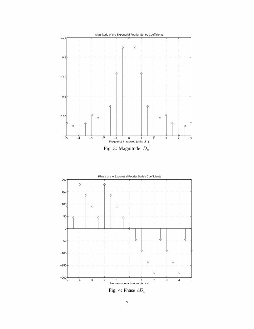
2) Plot the magnitude, |Dn| (in volts) and phase, Dn (in degrees) of the first thirteen coef-ficients (n = −6,−5, · · · , 6) versus frequency, ω (in rad/sec).
3) Using Parseval’s Theorem, find the (average) power in the signal’s first thirteen coeffi-cients. Express your answers in Watts and dBm.
1

Some warnings and comments: First, to find an expression for the Dn’s of g(t) you do NOThave to do an integration. Note, that g(t) is just a time shifted (delayed) symmetric trianglewave. The Dn’s for the symmetrical triangle wave are given in Appendix B. Next, the powerscalculated using Parseval’s Theorem assume a terminating resistance of 1 Ω (ohm). When youcompare these powers to the measured powers from the laboratory, you must adjust them (thecalculated Dn’s) because the spectrum analyzer assumes a 50 Ω termination.
Task:
Use the function generator to produce a triangular wave with unit amplitude (peak-to-peak 2volts) and a frequency of 1 MHz (or the maximum frequency allowed by the function generatorfor this type of signal). Verify that you have the correct waveform by displaying it on the oscil-loscope. Then, use the spectrum analyzer to examine the magnitude of this signal’s frequencyspectra. Measure and record the power (in dBm) of the fundamental (n = 1) and the next five(n = 2, 3, 4, 5, 6) harmonic components.
Data Analysis:
At each frequency component calculate the relative power (in dB) using the power at the fun-damental frequency (n = 1) as the reference. With powers measured in dBm the calculation ofthe relative power is quite straightforward as follows:
10 log∣∣∣∣ P
Pref
∣∣∣∣ = 10 log∣∣∣∣ P
1mW
∣∣∣∣ − 10 log∣∣∣∣ Pref
1mW
∣∣∣∣ ,
or in words,
Relative power (in dB) = Power of the component of interest (in dBm) − Power of the reference(in dBm).
2

Report:
For the pre-lab portion of your report, you should submit the following:
1) The “derivation” of the expression for Dn .
2) Plots (for n = −6,−1, · · · , 6) of
(a) |Dn| vs. ω.
(b) Dn vs. ω.
3) Two plots of the average power using Parseval’s Theorem for the first thirteen (n =−6,−1, · · · , 6) one in Watts and dBm.
For the laboratory portion of your report, produce a table for the data gleaned from measure-ments and those you calculated in the pre-lab. The table should have the following columns:
n Calculated*Power in dBm
Calculated* Powerrelative to n = 1 (in dB)
MeasuredPower in dBm
Measured Powerrelative to n = 1 (in dB)
......
......
...
* Including the adjustment for 50 Ω termination.
In your report, answer the following questions:
1) How close are the relative power columns – calculated and measured?
2) Does the power spectrum depend on the fundamental frequency? Explain!
3) What is the meaning of “n?” Why are there negative “n’s?”
4) Verify that the amplitude of the Fourier components for this waveform vary as (1/n2).
3

Appendix A to Lab #2
Calculating and Plotting Exponential Fourier Series Coefficients
Consider the periodic signal, g(t), shown below. The following tasks are performed usingMATLAB to do the numerical calculations and plots.
−2 −1 0 1 2 3 4 5 6 7 sec−0.5
0
0.5
1
1.5 Voltsg(t)
1) We want to evaluate the Fourier series coefficients using
Dn =1
4e−jn π
4 sinc(n
π
4
).
Plot the magnitude, |Dn| (in volts) and phase, Dn (in degrees) of the first twenty-onecoefficients ( n = −10,−9, · · · , 10) versus frequency (in rad/sec).
2) Plot two periods of g(t), directly–i.e., by creating a vector of samples of g(t) and plottingthat vector.
3) Plot an approximation to g(t) using these first twenty-one terms of the exponential Fourierseries.
An annotated copy of the MATLAB code used to generate the attached plots in Figures 3 and 4.
n = [-10:10]; % Sets up the vector of integer indices. The semicolon suppressed output to thescreen.
help exp
EXP Exponential.
EXP(X) is the exponential of the elements of X, e to the X.
For complex Z=X+i*Y, EXP(Z) = EXP(X)*(COS(Y)+i*SIN(Y)).
See also LOG, LOG10, EXPM, EXPINT.
z = n*(pi/4);
Dn = 0.25*exp(-i*z) .* sinc1(z); % The symbol “ .* ” means element-by-element multiply
4

magDn = abs(Dn); % Finds the magnitude of Fourier series coefficients
argDn = angle(Dn)*(180/pi); % Finds the phase (in degrees) of FS Coefficients
w=0.5*n;
stem(w,magDn),xlabel(’Frequency in rad/sec (units of pi)’),grid
title(’Magnitude of the Exponential Fourier Series Coefficients’)
stem(w,argDn),xlabel(’frequency in radians/sec (units of pi)’),grid
ylabel(’degrees’)
title(’Phase of the Exponential Fourier Series Coefficients’)The following code is used to find the sum given by
g(t) ∼=n=+10∑n=−10
Dnejnωt.
See Fig. 5. Note that explicit sum need not be calculated because we can use the properties ofmatrix multiplication to achieve the same result.
n = [-10:10];
nwo = n*(pi/2); % Defines the eleven frequencies of the sum
t = [0:0.01:8]; % Defines the time sampling points
BIG = nwo’ * t; % Creates a “big” matrix so we can use matrix multiplication to do the sum
g = Dn * exp(i*BIG); % Here’s where the sum is done
plot(t,real(g)),grid,xlabel(’Seconds’)
title(’Approximation to g(t) using the first ten components of the Fourier series’)The following code is used to generate two periods of the “real” function g(t). See Fig. 6.
It uses a unit step function, u(t), which is created in a homemade MATLAB function file. Acopy is shown below. The ability to use the unit step function to write piecewise functionsproves extremely efficacious when programming in MATLAB! Learn how to use it if you havenot done so in the past.
gt=(u(t) - u(t-1)) + (u(t-4) - u(t-5)) + u(t-8);
plot(t,gt)
grid,xlabel(’seconds’)
title(’The ”real” g(t)’)
axis([0 8 -0.2 1.2]);
% This changes the plot y-axis so it is the same as the previous plot of approximation to g(t).
5

Operations on the vector magDn can give power in Watts or dBm. However, care must be takenin interpreting the result of taking the logarithm since the magDn contains zeros. (Note, here aone-ohm termination has been assumed.)
Pave = magDn . 2 % Squares the elements of the vector of F.S. coefficient magnitudes
PdBm = 10*log10(Pave/1e-3)
The above powers have not been plotted here.
help log10
LOG10 Common (base 10) logarithm.
LOG10(X) is the base 10 logarithm of the elements of X.
Complex results are produced if X is not positive.
See also LOG, LOG2, EXP, LOGM.The following MATLAB code generates a unit step function and must be place in a file “u.m”.
function y=u(x)
y = 0.5 + 0.5*sign(x);The following MATLAB code generates a sinc function and must be place in a file “sinc1.m”.
function y=sinc1(x)
k=length(x);
for i=1:k
if x(i) == 0
y(i) = 1;
else
y(i) = sin(x(i))/x(i);
end
end
6
−5 −4 −3 −2 −1 0 1 2 3 4 50
0.05
0.1
0.15
0.2
0.25
Frequency in rad/sec (units of π)
Magnitude of the Exponetial Fourier Series Coefficients
Fig. 3: Magnitude |Dn|
−5 −4 −3 −2 −1 0 1 2 3 4 5−200
−150
−100
−50
0
50
100
150
200
Frequency in rad/sec (units of π)
Phase of the Exponetial Fourier Series Coefficients
Fig. 4: Phase Dn
7

0 1 2 3 4 5 6 7 8−0.2
0
0.2
0.4
0.6
0.8
1
1.2
seconds
Approximation to g(t) using the first ten components of the Fourier series
Fig. 5: Approximation of g(t)
0 1 2 3 4 5 6 7 8−0.2
0
0.2
0.4
0.6
0.8
1
Seconds
The "real" g(t)
Fig. 6: Real “g(t)”
8

Appendix B to Lab #2
Coefficients of Exponential Fourier Series for Some Often-Seen Periodic Signals
time
1.5Symmetric Triangle Wave
10.5
0−0.5−1−1.5
Period = T0
Dn =
sinc2(nπ/2), n = 00, n = 0
time
Period = T0
1.5
1
0.5
0
Pulse Width = τRectangular Pulse Train
Dn =τ
T0
sinc(nπ
τ
T0
)
9

time
1.510.5
0−0.5−1−1.5
Period = T0
Symmetric Sawtooth
Dn =
j (−1)n
nπ, n = 0
0, n = 0
Due date: Next lab session to your TA.
10

ECE 311 Communication Engineering
Lab Assignment #3
Fourier Series Coefficients using the FFT
Objective:
The purpose of this exercise is to introduce you to the FFT (Fast Fourier Transform) as a methodof finding the (exponential) Fourier series coefficients of a periodic function. You will useMATLAB to calculate the coefficients using both the FFT algorithm and the theoretical formula.In the lab, you will generate the waveform and use the oscilloscope’s FFT module to look at thesignal’s spectra.
You will learn the following:
1) How to interpret the output of the FFT, the spacing, the range, and the location of thepositive and negative parts of the frequency components; and
2) The effects of the sampling rate and number of samples on the output.
Introduction:
Read textbook Sections 2.10 and 3.9 (especially Computer Examples C3.1 and C3.2). A usefulreview of FFT theory as it relates to the Agilent (Hewlett-Packard) oscilloscope module you willuse in the lab can be found at http://www.educatorscorner.com/experiments/pdfs/exp53a.pdf.
Pre-Lab:
Use MATLAB’s FFT and FFTSHIFT functions to find the (exponential) Fourier series for thesignal given below. Use two periods of the signal with a total of 128 sample points.
time
1.510.5
0−0.5−1−1.5
g(t)
T = 1 sec0
Dn =
j (−1)n
nπ, n = 0
0, n = 0
1

Plot the magnitude (in volts) of Fourier series coefficients vs. frequency (in Hertz) using thefollowing guidelines.
a) Arrange the plot such that the DC component (n = 0) is at the center. (This involvesusing the MATLAB function FFTSHIFT.)
b) Plot the terms for n = −5,−1, · · · , 5 only.
c) The plot should be vs. frequency in Hertz. (See the comment that follows.)
d) Calculate the magnitude (in volts) of the theoretically calculated (referred to in the follow-ing as “actual”) coefficients given by the formula. Do this for the terms n = −5,−4, · · · , 5.Plot these magnitudes using the same axis as Part (c).
e) In addition to the plots, record the FFT and “actual” amplitudes (in volts) at the frequencycomponents for n = 1, 2, 3, 4, 5 . Tabulate your data as shown the report requirement.
Comment on the Frequency Axis for the Plots:
This is the most confusing vectors to create because of how the FFT “scrambles” its output.But, without proof, it can be shown by a hard working student, that the frequency vector againstwhich the shifted FFT, created by FFTSHIFT, should be plotted, is given as follows:
f = ∆fn − 1 − N
2
f = vector of frequencies
∆f = the frequency increment
n = a vector of integers from 1 to N
N = the number of samples in the vector used for the FFT.
Thus, the MATLAB code to generate the initial plot of Fourier series coefficient magnitudes vs.frequency is
plot(f , abs(FX))where FX is the output vector from the FFTSHIFT MATLAB function.
This plot will look a little “cramped” and you will want to “zoom-in” on the middle elementsof the vector. For help on doing this see the MATLAB manual and try typing “help axis.”
Task:
In the lab, generate the periodic waveform shown above except make the fundamental frequency100 kHz. Display it on channel 1 of the oscilloscope using a 50 Ω termination. Use the FFTmodule on the oscilloscope to view and measure the amplitude spectra of the periodic wave-form. Measure the amplitudes and frequencies for n = 1, 2, 3, 4, 5 components. Record thisdata.
2

The FFT function appears in a soft key menu under the ± (math) button. There are two mathfunction choices under this button, F1 and F2. The FFT is available with the F2 choice. (Turnit ON, press MENU, and choose FFT under OPERATION.) Once FFT is chosen, to get a betterlooking frequency plot, turn OFF the channel one, time-domain display by pressing the “1”button a couple of times.
The FFT menu has a number of soft keys. Use the default settings for most of the options, butmake sure you use the FLATTOP choice in the WINDOWS soft key for amplitude measure-ments and the HANNING choice for frequency measurements.
The frequency axis span is adjusted using the time/division knob. Since only amplitudes arebeing displayed and you only have to measure the positive frequency components, you can setDC (0 Hz) to the left of the screen.
The amplitude axis is logarithmic with units in dBV with 1 volt RMS as the reference. Pressingthe cursor button activates the cursors with amplitudes displayed in dBV. Pressing the FINDPEAKS soft key automatically puts the cursors at the two largest spectral lines on the screen.Cursors can be selected using the soft keys and manually moved using the cursor knob.
Data Analysis:
Convert the lab data from dBV to volts. First, convert the data to RMS voltages (VRMS) byinverting the definition of dBV, i.e., dBV = 20 log (VRMS). Second, adjust the RMS voltage topeak voltages (VP ) by multiplying by 1.414 (why?). Finally, this peak value must be dividedby a factor of two. This factor of two is necessary because, when the oscilloscope FFT modulepresents the data at a given frequency, it sums the magnitude of the coefficients at both negativeand positive frequencies. The number resulting from this procedure will be referred to as the“measured” value for the coefficient.
Next, using the “actual” amplitude as the reference, find the percentage error for each compo-nent’s amplitude “computed” using MATLAB’s FFT and “measured” using the oscilloscope’sFFT module. Put your results in the appropriate row and column in the table below. Recall that
Percentage error = 100 × |(test value – reference value)/reference value)|.Report:
For your report, submit the two graphs from your pre-lab and your analyzed data tabulated asshown below. As always, your report should start with a cover sheet and end with a copy of theraw data you took in the laboratory.
n “Actual”Amplitudes(Volts)
“Computed” FFTAmplitudes(Volts)
PercentageError forMATLAB
“Measured” FFTAmplitudes(Volts)
PercentageError forMeasured
......
......
......
Due date: Next lab session to your TA.
3

ECE 311 Communication Engineering
Lab Assignment #4
Investigation of a Simple Filter
Objective:
The purpose of this experiment is to investigate the frequency response of a simple linear system(a filter) and to use it to predict the system’s output for a periodic input signal. We note thatin this experiment a deterministic, periodic signal is used to do this investigation in order tofacilitate the use of laboratory equipment to make measurements. In communication systemsthe information that is filtered is random and non-deterministic.
You should calculate a theoretically expected frequency response for the circuit given for thisexperiment. Using this result, you can then predict the effect this filter has on the spectrum ofthe input. A computer simulation should verify the results of this prediction.
In the laboratory, you should build and test the circuit. In particular, you want to verify theresults of the calculation and simulation, by looking at the ratio of the output Fourier seriescoefficients to the input Fourier series coefficients.
Introduction:
The block diagram for a single-input, single-output linear system is shown below. If the systemis asymptotically stable and we are interested in the operation of the system in the steady-state, the system’s frequency response, H(ω), shows how the system modifies the input signal’sspectrum. In this case, we call the system a filter. For this experiment, review the appropriatematerial on linear systems and frequency response from your linear system’s course (ECE 310).
g(t)h(t), H(s), H (ω)
y(t)
(ω)Y(s), YG(s), G (ω)
A block diagram
For linear systems, we have
H(s) =Y (s)
G(s), H( ω ) = H(s)|s=jω .
Note, that in this experiment the frequency response will be evaluated at the discrete frequenciesof the input signal’s spectrum. For a linear system with a periodic input, the input and outputset of frequencies are the same. The only thing that a linear system “does” is to change themagnitude and phase of the spectra at those frequencies.
In appendix A, a simple filter is analyzed. H(ω) is calculate, the MATLAB code used to generateplots of H(ω) is given, and the issue of scaling is discussed. In appendix B, the filter of appendixA is simulated using PSpice and its frequency response is found.
1

Pre-Lab:
Theoretical Calculation
Find an expression for H(ω), the circuit’s (shown in the figure) frequency response. Use MAT-LAB to plot its magnitude |H(ω)| (in dB) and phase angle H(ω) (in degrees) for the funda-mental frequency (f0) and the first seven harmonics (f = nf0; n = 1, 2, · · · , 8). Remember that“f” is in Hertz (cycles/second) and “ω” is in radians/second and that ω = 2πf .
A circuit
Simulation
Simulate the circuit for this experiment using Pspice. You can use Pspice to find the circuit’sfrequency response, and therefore check the results of your theoretical calculation. This is doneby using the “AC Sweep” option under the “Analysis” menu.
Tasks:
Build the circuit, excite the circuit with the input signal shown below and do the followingmeasurements.
Use the spectrum analyzer to measure the magnitude (in dBm) of the Fourier series coefficientsof the signal without the filter inserted in the circuit. Make this measurement for the fundamen-tal frequency and the first seven harmonics (f = nf0; n = 1, 2, · · · , 8). Next, insert the filterinto the circuit and repeat the measurements for the same frequencies used without the filter.Record your measurements.
2

The rectangular pulse train input signal:
DC offset = 0 voltsPulse Amplitude = 5 volts (peak-to-peak)Duty Cycle = 20%Period = 1 microsecond
Period = T
0
0.5
1
1.5
time
pulse width = τGeneric rectangular pulse train
Analyzing the Data:
Next, for the pair of data points at each frequency subtract measurement taken with the filterin the circuit from that taken without the filter. This gives you the magnitude of the circuit’sfrequency response, its attenuation, at that frequency (the fundamental and integer multiplesof it). This should be compared with those attenuations obtained from the calculations andsimulation.
Tabulate your data as follows:
Measured Calculated Simulatedn frequency
(nω0)input(dBm)
output(dBm)
|H(nω0)|(dBm)
|H(nω0)|(dB)
|H(nω0)|(dB)
12345678
3

Report:
First, each group should submit the work they did on the theoretical calculations and simula-tions. For the theoretical calculations this should include (i) your calculation of H(ω), and (ii)your MATLAB plots of |H(ω)| and H(ω). For the simulation, include plots of |H(ω)| and H(ω) found using the “AC sweep” analysis. The frequency axes for all plots should be inHertz.
Then, each group should submit the measurements they took in the laboratory. This shouldinclude the table shown above and a few words commenting on “how close were your calcula-tions.” Is there a systematic difference between the measured results and those obtained fromMATLAB and PSpice? Explain.
4

ECE-311
Appendix A to Experiment #4
Frequency Response of a Simple RC Filter
Suppose we want to find the frequency response of the filter shown in Figure 1.
Fig. 1: Schematic diagram of a simple lowpass filter
The system’s (circuit’s) s-domain transfer function, H(s), can be found by doing nodal analysis,assuming Vin(s) is known, solving for Vout(s) in terms of Vin(s), and taking their ratio to getH(s). The transfer function is
H(s) =1/R1R2C1C2
s2 +(
1R2C2
+ 1R1C1
+ 1R2C1
)s + 1
R1R2C1C2
Volts/Volt.
Upon substituting the given capacitor and resistor values and letting s = jω, circuit’s frequencyresponse is found (after collecting numerator and denominator into real and imaginary parts) tobe
H (ω) =0.1 × 10¹²
[0.1 × 10¹² − ω2] + j [1.2 × 10⁶ω]Volts/Volt.
Now, suppose we want to plot the magnitude |H(ω)| and phase H(ω) of the frequency re-sponse from DC to 1 MHz (2π Megaradians/second.) You could do this as it stands, but tosimplify the calculation and diminish errors in the numerical computation, you should scalethis function by 106 radians/second. In essence, we are making a change to a new variable,ωx, which has a unit measure of 1 Megaradians/second. This means that ω = 106ωx, i.e., oneunit of ωx is 106 units of ω. Making this change of variable and simplifying gives a scaled thefrequency response
H (ω) =0.1
[0.1 − ω2] + j [1.2 ω]Volts/Volt.
5

It is this function that is used in the following MATLAB code to generate the plots of Figures 2through 4.
w = 0:0.05:2*pi; %Sets up a vector of frequencies.
NUM = 0.1; %Here’s the numerator function.
DEN = (0.1 - w . 2) + j*1.2*w; %Here’s the denominator.
Hw =NUM ./ DEN; %These are complex numbers.
plot(w,abs(Hw)),grid %Produces Figure 2
title(’Magnitude of Frequency Response’),xlabel(’megaradians/sec’)
ylabel(’Volts/Volt’)
magdB = 20*log10(abs(Hw)); %Converts to decibels
plot(w,magdB),grid %Produces Figure 3
title(’Magnitude of Frequency Response’),xlabel(’megaradians/sec’)
ylabel(’decibel’)
phase = angle(Hw)*180/pi; %Changes radians to degrees
plot(w,phase),grid %Produces Figure 4
title(’Phase of Frequency Response’),xlabel(’megaradians/sec’)
ylabel(’degrees’)
6

0 1 2 3 4 5 6 70
0.1
0.2
0.3
0.4
0.5
0.6
0.7
0.8
0.9
1Magnitude of Frequency Response
megaradians/sec
Vol
ts/V
olt
Fig. 2: Magnitude of the filter’s frequency response (in Volts/Volt)
0 1 2 3 4 5 6 7−60
−50
−40
−30
−20
−10
0Magnitude of Frequency Response
megaradians/sec
deci
bel
Figure 3: Magnitude of the filter’s frequency response (in dB)
7

0 1 2 3 4 5 6 7−180
−160
−140
−120
−100
−80
−60
−40
−20
0Phase of Frequency Response
megaradians/sec
degr
ees
Figure 4: Phase of the filter’s frequency response
8

ECE-311
Appendix B to Experiment #4
Information on Doing PSpice Simulations
Installing and Running PSpice on the ACCC Machines:
Version 8 of PSpice is available on the ACCC PC’s, but it usually has to be installed on the serveryou are using. (Sometimes someone else on the same server has already installed PSpice, butthis is NOT common. If it is installed, the installing program will tell you.)
To install PSpice use the following menu path to get to the installing program: Start → Programs→ ACCC Software Installer → ACCC Network Installer. Click on ACCC Network Installer“menu item.” Find PSpice 8 and highlight it. Click on the “install” button.
To run PSpice use the following menu path to get the schematic capture front-end of PSpice:Start → Programs → Class Apps → PSpice → Schematics. Click on the “Schematics” menuitem.
Simulation of the Simple Filter of Appendix A to Obtain Its Frequency Response:
It is assumed that you have had some exposure to PSpice. For those who need a review, a goodintroduction and reference from which to learn is the book Schematic Capture Using MicroSimPSpice for Windows 95/98/NT by Marc E. Herniter (Prentice-Hall).
What follows are copies of various PSpice windows used to do the analysis for and generateplots of H(f) – |H(f)| and H(f), the magnitude and phase of the frequency response. PSpiceuses Hertz as the frequency variable; therefore, a certain amount of interpretation is neededwhen the output is viewed. The output is viewed using the PSpice’s graphical output, Probe.
The following circuit was “built” using PSpice’s schematic capture front-end, Schematics. Ifyou are not familiar with creating circuit diagrams using Schematics, seek the help of yourteaching assistant for some initial guidance or refer to the book referenced above.
9

The voltage marker at the output node tells Probe to automatically display this node voltageafter the simulation is finished. The analog ground (AGND) is needed for PSpice to do theanalysis.
In order to do a frequency response simulation, you must use “VAC” as the voltage source.Note, that if you set the amplitude of the voltage source equal to one and its phase equal to zero,the plot of a particular node voltage as a function of frequency will be the frequency response(in volts/volt vs. Hertz) of the circuit, considering the voltage source as the input and the nodeas the output. Next, you must enable the “AC Sweep” from the Analysis → Setup menu andchoose the frequency range and intervals.
The following dialog box is activated with “AC Sweep” button, above. You can choose the typeof sweep, the start frequency, the stop frequency, and the number of data points to be calculated.Frequencies are in Hertz. Usually, for a narrow band of frequencies, a linear sweep is used. Fora broad band of frequencies, a decade sweep is used. A certain amount of “playing around” isencouraged in order to make your output “look pretty.” If your output looks jagged, you havenot chosen enough points.
10

Once you have correctly “built” the circuit, with the proper AC input source and with the outputnode identified with a voltage marker, and once you have enabled the “AC Sweep” and chosena frequency range, you are ready to do the simulation. This is activated by clicking on the menupath: Analysis → Simulate.
The result of the simulation is plotted by Probe and is shown below. Because we chose theinput voltage amplitude to be one volt, this trace is the magnitude of the frequency response.
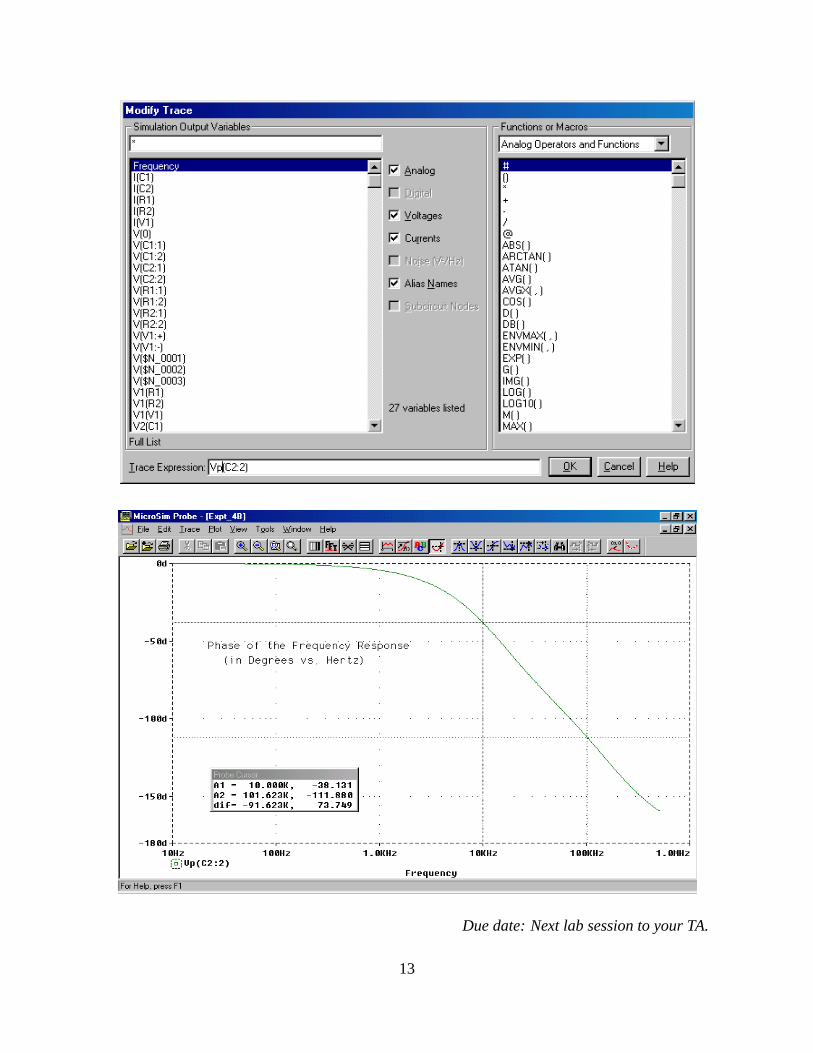
To get the plot in dB you double click on output voltage variable label, V(C2:2), located in thelower left-hand corner of the Probe window. When the “Modify Trace” window appears, inthe Trace Expression box change the label to Vdb(C2:2). This window and the resulting plotchange are shown on the next two figures.
To get the phase plot you double click on output voltage variable label, V(C2:2), located in thelower left-hand corner of the Probe window. When the “Modify Trace” window appears, inthe “Trace Expression” box change the label to Vp(C2:2). This window and the resulting plotchange are shown after next two figures.
The plots on the next two pages also show cursors, which can be used to identify the coordinatesof points on the trace. The cursors are activated by the “Cursor Toggle” button on the toolbar.The A1 cursor is controlled by the left mouse button and the A2 by the right.
11

12
Due date: Next lab session to your TA.
13

ECE 311 Communication Engineering
Lab Assignment #5
Examination of DSB-LC (Broadcast AM) Spectra
Objective:
In this project, you will investigate the broadcast form of amplitude modulation (AM), doublesideband large carrier (DSB-LC). To do this you will use MATLAB and Pspice, with their FFTcapabilities, to investigate the expected time-domain waveform and the expected frequency do-main spectra of single-tone modulated AM signals. In the laboratory, you will use the functiongenerator to produce these AM signals and to examine their time domain signals and its spectra.
Introduction:
Read Sections 4.1 through 4.3 in the text for the theory underlying DSB-LC (AM) modulation.The settings needed to produce these AM signals in the laboratory are discussed in the followingsections of the function generator’s User’s Guide: Chapter 2, pp. 41–43; Chapter 3, pp. 71–75;Chapter 7, pp. 283–288.
Review the material from experiment #3 on interpreting the FFT. An appendix is attached thatdiscusses the PSpice simulation of AM signals.
Pre-Lab:
Part I
Using MATLAB, plot the time domain representation and the magnitude of its Fourier trans-form, obtained using the FFT routine, for the two traditional AM signals (DSB-LC), shownbelow,
ϕam(t) = [1 + µ cos(8πt)]2 cos(64πt), µ = 0.2, 0.8.The horizontal scale for the FFT output should be in Hertz. Answer the following questions forboth signals.
a) Use the time-domain AM signal to find “µ,” its modulation index. Is it right?
b) Compare the FFT output to what is theoretically expected.
i) What were the frequencies of the carrier and sidebands?
ii) What is the total power in the signal (in dBm)?
iii) What is the power in the carrier and sidebands (dBm)?
iv) What are the relative powers of the sidebands with respect to the carrier (in dB)?
Note, that the spectra of these signals will be “delta functions”, your choice of N , Ts , and To
must be made carefully so as to avoid the “picket fence” effect associated with the DFT.
1

Part II
Using Pspice, simulate the DSB-LC signal, shown below,
ϕam(t) = [1 + µ cos(2πfmt)]2 cos(2πfct), µ = 0.2, 0.8
where fm = 20 kHz and fc = 1 MHz.
Plot the time domain output and its FFT-generated magnitude spectra.
a) Use the time-domain AM signal to find “µ,” its modulation index. Is it right?
i) Compare the FFT output to what is theoretically expected.
ii) What were the frequencies of the carrier and sidebands?
iii) What is the total power in the signal (in dBm)?
iv) What is the power in the carrier and sidebands (dBm)?
v) What are the relative powers of the sidebands with respect to the carrier (in dB)?
Task:
Use the function generator to generate two single-tone modulated AM waveforms with the spec-ifications given below. Use the “Front-Panel Operation” outlined in the User’s Guide referencedabove. For each AM signal, do the following.
a) Examine the output using the oscilloscope. Sketch the waveform and use this informationto find the index of modulation. Is it what you expected?
b) Next use the spectrum analyzer to find the power in the signal – the carrier and the side-bands. Compare these to the calculated values.
i) Are the frequencies what you expected?
ii) Are the powers what you expected?
iii) Are the relative values – sidebands with respect to the carrier what you expected?
Signal Specifications:
Carrier: Frequency = 1 MHz, Amplitude = 4 volts (p-p)Modulating Tone: Sinusoid at 20 kHzIndex (Depth) of Modulation: 20% and 80%
Data Analysis:
Determine the percentage error for the two indices of modulation you calculated from the timedomain AM signals that you displayed in each of the three methods you used – MATLAB,PSpice, and Function Generator – to generate the waveform.
2

Determine the efficiency, n, of the AM transmission for the two indices of modulation youused for this experiment. Calculate a theoretically expected efficiency and the actual efficiencyfrom the sideband and carrier power data you obtained in the lab or from the simulations. Theefficiency formulas are as follows:
ηactual =PS
PS + PC
100%, ηtheoretical =µ2
2 + µ2100%
where Pc = carrier power in Watts and Ps = total sideband power in Watts.
Report:
In your report, answer the questions concerning the comparison of the calculated and measuredvalues of indices of modulation, powers of the carrier and sidebands, and the frequencies of thecarrier and sidebands.
Summarize your analyzed data in following table:
Expected MATLAB PSpice Laboratory Measurements
µ = 0.2
Ps/Pc (in dB) *η
% error in µ
µ = 0.8
Ps/Pc (in dB)η
% error in µ
* Here Ps is the power in one sideband.
3

ECE-311
Appendix A to Experiment #5
Simulating Linear Modulation in PSpice
The above schematic can be “built” in PSpice. It uses a function block, MULT, which just doesthe time domain multiplication of two input signals. MULT can be found in the ABM libraryof PSpice. The voltage sources are VSIN with the attributes assigned as indicated above. Thecircuit needs a load resistor and an analog ground to work.
“Transient” simulation is done (with Print Step = 20m and Final Time = 2). This is foundunder the “Analysis Setup” menu. The output, taken across the 1 kΩ resistor, is automaticallydisplayed in Probe. Its FFT may be obtained by clicking on the “FFT Icon” on the Probetoolbar.
The mathematical expression for the output voltage is as follows:
Vout(t) = [1 + 0.5 sin(2πt)] sin(20πt)
Vout(t) = 1 sin(20πt) + 0.25 cos(18πt) + 0.25 sin(22πt).
4

Time-domain output is shown in the next figure.
The FFT of the above signal is shown next (Here we have “zoomed-in” on the important part ofthe spectra).
Compare the magnitude of the FFT coefficients and the last Vout(t) expression given above.Note that like the oscilloscope’s FFT module, the PSpice version calculates the magnitude ofthe compact trigonometric Fourier Series coefficients. No phase information is given.
Due date: Next lab session to your TA.
5

ECE-‐311 Experiment #7
The Detection of AM Signals Objective: The purpose of this experiment is to investigate the two major forms of AM demodulation, coherent (synchronous) detection and non-‐coherent detection. You will generate a single-‐tone modulated AM signal using the function generator and use these two methods to recover the modulating tone. These two methods use different circuits which you will be asked to design and build. The coherent detection method uses the balanced modulator circuit from the last laboratory experiment and a simple RC low-‐pass filter that you will design. The non-‐coherent detection method uses an envelope detector circuit, which you will design. Introduction: Read that part of section 4.3 in the text, which discusses AM demodulation. Focus your attention on the design of an envelope detector detailed in Example 4.6. Problem 4.3-‐1 shows the block diagram for a synchronous AM demodulator. If you have not, as of yet, done this problem, do it and compare your solution to the answer book’s. Pre-‐Lab: For this experiment, you must design a envelope detector for non-‐coherent detection method. Also, you must design the circuit for the low-‐pass filter block of the synchronous demodulator. Do this prior to lab. For this design you should find actual component values (numbers), not just the formulas for them. Note, that you are trying to detect an AM signal modulated (μ = 0.5) with a 2 KHz tone. Simulate both your designs using PSpice. Task: Part One (Synchronous Detection) Build and test the synchronous detection circuit shown below. There are two inputs for the balanced modulator, the AM signal and the local oscillator signal. Their specification is given below. Use one function generator to produce the AM signal and the other to produce the local oscillator signal. In order for synchronous detection to work properly these two generators must be synchronized! As shown in figure 2, this can be done via a connection on the back of the two function generators. Your teaching assistant will show you how to do this. Connect the output of the demodulator to the oscilloscope (AC coupling with high input impedance). Did you get the 2 kHz modulating sinusoid at the output?
AM signal: fC = 1 MHz, fm = 2 KHz (sinusoid) μ = 0.5 VRMS < 300 mV
Local Oscillator: fLO = 1 MHz VRMS < 60 mV

Figure 1 – Synchronous Detection

Part Two (Envelope Detector) Build and test the envelope detector shown in figure 3. In the pre-lab, you were to determine the values (i.e. numbers) for R and C. Here you don’t need the synchronized local oscillator. The only input needed is the AM signal. Use the same specifications as Part One, EXCEPT adjust the amplitude of the AM signal so that its “envelope valley voltage” is greater than the diode’s “cut-in” voltage ( 0.7 volts). Did you get the 2 kHz modulating sinusoid at the output?
Figure 3 – Envelope Detector 1N4148 (or equivalent*)
AM Signal To Oscilloscope C R (*Any small-signal diode may be used.) Both Parts For both parts, have your teaching assistant verify that your detectors “worked.” There may be a certain amount of “tweaking” (adjusting component values) needed to make the detectors operational. Data Analysis: Report: In your report, include the following:
• The design component values, from the pre-lab calculations, for both detectors, • The simulations used to “test” your designs, and • The actual design values you used.
Also, include a brief discussion of the advantages and disadvantages of both methods of detection.
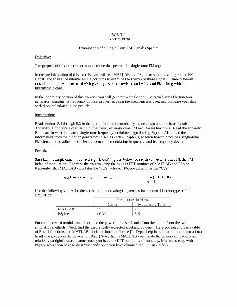
ECE-311Experiment #8
Examination of a Single-Tone FM Signal’s Spectra
Objective:
The purpose of this experiment is to examine the spectra of a single-tone FM signal.
In the pre-lab portion of this exercise you will use MATLAB and PSpice to simulate a single-tone FMsignals and to use the internal FFT algorithms to examine the spectra of these signals. Three different
intermediate case.
In the laboratory portion of this exercise you will generate a single-tone FM signal using the functiongenerator, examine its frequency domain properties using the spectrum analyzer, and compare your datawith those calculated in the pre-lab.
Introduction:
Read sections 5.1 through 5.3 in the text to find the theoretically expected spectra for these signals.Appendix A contains a discussion of the theory of single-tone FM and Bessel functions. Read the appendixB to learn how to simulate a single-tone frequency modulated signal using Pspice. Also, read theinformation from the function generator’s User’s Guide (Chapter 3) to learn how to produce a single-toneFM signal and to adjust its carrier frequency, its modulating frequency, and its frequency deviation.
Pre-lab:
FM
index of modulation. Examine the spectra using the built-in FFT routines of MATLAB and PSpice.Remember that MATLAB calculates the “Dn’s” whereas PSpice determines the “Cn’s.”
FM ! " #c $ #mt ] %&'( ( (&)
A = 1
Use the following values for the carrier and modulating frequencies for the two different types ofsimulations
Frequencies in HertzCarrier Modulating Tone
MATLAB 32 2PSpice 1.0 M 5 K
For each index of modulation, determine the power in the sidebands from the output from the twosimulation methods. Next, find the theoretically expected sideband powers. (Here you need to use a tableof Bessel functions and MATLAB’s built-in function “besselj”. Type “help besselj” for more information.)In all cases, express the powers in dBm. (Note, that in MATLAB you can do the power calculations in arelatively straightforward manner once you have the FFT output. Unfortunately, it is not so easy withPSpice where you have to do it “by hand” once you have obtained the FFT in Probe.)

Task:
Use the function generator to generate a single-tone modulated FM waveform with the specifications givenbelow. Use the spectrum analyzer to find the power in the signal — the carrier and the sidebands — (indBm).
Signal Specifications:Carrier: Frequency = 1 MHz Amplitude = 2 volts (p-p)Modulating Tone: Sinusoid at 5 kHzIndex of Modulation: %&'( ( (&)
(Note that the function generator does NOT have a direct adjustment to *'+ , *- ./ '+ '
Data Analysis:
Normalize your data using the total power available in an FM signal as a reference. Recall that the totalpower in an FM signal is constant ( = A2/2R). For the signals in the pre-lab, R = 1 and PTOTAL = 0.5 W (27dBm). Thus, for these pre-lab signals, the normalized power (in dB) is the calculated power (in dBm)minus 27. For the signals measured in the laboratory, R = 50 and PTOTAL = 10 mW (10 dBm). Thus, forthese laboratory signals, the normalized power (in dB) is the measured power (in dBm) minus 10.
Choose those sidebands with powers that are greater than or equal to 1% of the total power in the FMsignal. Use these sidebands to determine the signal’s bandwidth. Note, that those sidebands with relativepowers greater than –20 dB meet the 1% criteria for inclusion in the bandwidth calculation. (Verify thisstatement for yourself. It could be a good test question!!)
Report:
On a separate sheet of paper for each index of modulation, tabulate your above calculations using thefollowing template.
Relative Powers (in dB)n Frequency (Hz) Theory PSpice MATLAB Measured
BW =(Theory)
BW = (PSpice)
BW =(MATLAB)
BW = (Measured)
BW =(Carson’s Rule)
Here the bandwidth (BW) you state should be normalized to the modulating frequency – i.e.,BW = “real” bandwidth ÷ fm
Also, accompanying each sheet include another sheet with plots of the MATLAB and PSpice FFT outputs,zoomed-in as appropriate.

ECE-311Appendix A to Experiment #8
Bessel Functions and Single-Tone FM
A single-tone FM signal may expanded in a Fourier series as follows:
FM ! " #c $ #mt ]
( )[ ]∑+∞=
−∞=+=
n
nmcFM tnAt ωωϕ cos)(J)( n
where the Jn(x)’s are a discrete infinite set, indexed by the integer “n,” of real-valued functions of a realvariable. These are called the Bessel Functions of the First Kind. Bessel functions occur in a number ofapplications in mathematical physics. Formulas for evaluating the functions have been developed and canbe found in any standard mathematical handbook. A useful tabulation of a number of Bessel Functionvalues at various values of the argument is attached. This tabulation can be used for negative indices byusing the following property of the Bessel Functions:
Jn(x) = (–1)nJ–n(x) .
In reference to the single-tone FM signal, it has been represented as an infinite number of sinusoidscentered at the carrier frequency (fc), with a frequency spacing determined by the modulating frequency(fm). The index “n” determines the frequency of the sideband, fsideband = fc + nfm (n = 0 is the carrier). Theamplitude of the signal component at that frequency is determined by the nth order Bessel Function valuewhere the argument is the signal’s index of modulation ' 0 / 1!2n13 4n’s FM(t).
As an example, suppose a unit amplitude 100 kHz (fc) sinusoid is frequency modulated with a 5 kHz (fm)tone and an index of modulation of 8. (Note, this signal is simulated using PSpice in Appendix B.) Whatis the power in the signal at 80 kHz?
Since fsideband = 80 kHz and fsideband = fc + nfm , then n = –4. The amplitude of the sinusoid at 80kHz is
|1•J–4(8)| = 0.110
This compares favorable with the spectra plot of Appendix B. To calculate the power associatedwith the signal at 80 kHz, we use A2/2 where is “A” is the amplitude of the sinusoidal componentof the signal at 80 kHz – i.e., 0.110. Thus, the power is 6.05 mW (7.82 dBm).

Bessel Functions of the First Kind, Jn(x)x= n = 0 1 2 3 4 5 6 7 8 9 100.0 1.00 0.00 0.00 0.00 0.00 0.00 0.00 0.00 0.00 0.00 0.000.2 0.99 0.10 0.00 0.00 0.00 0.00 0.00 0.00 0.00 0.00 0.000.4 0.96 0.20 0.02 0.00 0.00 0.00 0.00 0.00 0.00 0.00 0.000.6 0.91 0.29 0.04 0.00 0.00 0.00 0.00 0.00 0.00 0.00 0.000.8 0.85 0.37 0.08 0.01 0.00 0.00 0.00 0.00 0.00 0.00 0.001.0 0.77 0.44 0.11 0.02 0.00 0.00 0.00 0.00 0.00 0.00 0.001.2 0.67 0.50 0.16 0.03 0.01 0.00 0.00 0.00 0.00 0.00 0.001.4 0.57 0.54 0.21 0.05 0.01 0.00 0.00 0.00 0.00 0.00 0.001.6 0.46 0.57 0.26 0.07 0.01 0.00 0.00 0.00 0.00 0.00 0.001.8 0.34 0.58 0.31 0.10 0.02 0.00 0.00 0.00 0.00 0.00 0.002.0 0.22 0.58 0.35 0.13 0.03 0.01 0.00 0.00 0.00 0.00 0.002.2 0.11 0.56 0.40 0.16 0.05 0.01 0.00 0.00 0.00 0.00 0.002.4 0.00 0.52 0.43 0.20 0.06 0.02 0.00 0.00 0.00 0.00 0.002.6 -0.10 0.47 0.46 0.24 0.08 0.02 0.01 0.00 0.00 0.00 0.002.8 -0.19 0.41 0.48 0.27 0.11 0.03 0.01 0.00 0.00 0.00 0.003.0 -0.26 0.34 0.49 0.31 0.13 0.04 0.01 0.00 0.00 0.00 0.003.2 -0.32 0.26 0.48 0.34 0.16 0.06 0.02 0.00 0.00 0.00 0.003.4 -0.36 0.18 0.47 0.37 0.19 0.07 0.02 0.01 0.00 0.00 0.003.6 -0.39 0.10 0.44 0.40 0.22 0.09 0.03 0.01 0.00 0.00 0.003.8 -0.40 0.01 0.41 0.42 0.25 0.11 0.04 0.01 0.00 0.00 0.004.0 -0.40 -0.07 0.36 0.43 0.28 0.13 0.05 0.02 0.00 0.00 0.004.2 -0.38 -0.14 0.31 0.43 0.31 0.16 0.06 0.02 0.01 0.00 0.004.4 -0.34 -0.20 0.25 0.43 0.34 0.18 0.08 0.03 0.01 0.00 0.004.6 -0.30 -0.26 0.18 0.42 0.36 0.21 0.09 0.03 0.01 0.00 0.004.8 -0.24 -0.30 0.12 0.40 0.38 0.23 0.11 0.04 0.01 0.00 0.005.0 -0.18 -0.33 0.05 0.36 0.39 0.26 0.13 0.05 0.02 0.01 0.005.2 -0.11 -0.34 -0.02 0.33 0.40 0.29 0.15 0.07 0.02 0.01 0.005.4 -0.04 -0.35 -0.09 0.28 0.40 0.31 0.18 0.08 0.03 0.01 0.005.6 0.03 -0.33 -0.15 0.23 0.39 0.33 0.20 0.09 0.04 0.01 0.005.8 0.09 -0.31 -0.20 0.17 0.38 0.35 0.22 0.11 0.05 0.02 0.016.0 0.15 -0.28 -0.24 0.11 0.36 0.36 0.25 0.13 0.06 0.02 0.016.2 0.20 -0.23 -0.28 0.05 0.33 0.37 0.27 0.15 0.07 0.03 0.016.4 0.24 -0.18 -0.30 -0.01 0.29 0.37 0.29 0.17 0.08 0.03 0.016.6 0.27 -0.12 -0.31 -0.06 0.25 0.37 0.31 0.19 0.10 0.04 0.016.8 0.29 -0.07 -0.31 -0.12 0.21 0.36 0.33 0.21 0.11 0.05 0.027.0 0.30 -0.00 -0.30 -0.17 0.16 0.35 0.34 0.23 0.13 0.06 0.027.2 0.30 0.05 -0.28 -0.21 0.11 0.33 0.35 0.25 0.15 0.07 0.037.4 0.28 0.11 -0.25 -0.24 0.05 0.30 0.35 0.27 0.16 0.08 0.047.6 0.25 0.16 -0.21 -0.27 -0.00 0.27 0.35 0.29 0.18 0.10 0.047.8 0.22 0.20 -0.16 -0.29 -0.06 0.23 0.35 0.31 0.20 0.11 0.058.0 0.17 0.23 -0.11 -0.29 -0.11 0.19 0.34 0.32 0.22 0.13 0.068.2 0.12 0.26 -0.06 -0.29 -0.15 0.14 0.32 0.33 0.24 0.14 0.078.4 0.07 0.27 -0.00 -0.27 -0.19 0.09 0.30 0.34 0.26 0.16 0.088.6 0.01 0.27 0.05 -0.25 -0.22 0.04 0.27 0.34 0.28 0.18 0.108.8 -0.04 0.26 0.10 -0.22 -0.25 -0.01 0.24 0.34 0.29 0.20 0.119.0 -0.09 0.25 0.14 -0.18 -0.27 -0.06 0.20 0.33 0.31 0.21 0.129.2 -0.14 0.22 0.18 -0.14 -0.27 -0.10 0.16 0.31 0.31 0.23 0.149.4 -0.18 0.18 0.22 -0.09 -0.27 -0.14 0.12 0.30 0.32 0.25 0.169.6 -0.21 0.14 0.24 -0.04 -0.26 -0.18 0.08 0.27 0.32 0.27 0.179.8 -0.23 0.09 0.25 0.01 -0.25 -0.21 0.03 0.25 0.32 0.28 0.1910.0 -0.25 0.04 0.25 0.06 -0.22 -0.23 -0.01 0.22 0.32 0.29 0.21

ECE-311Appendix B to Experiment #8
Generating an FM signal in PSpice
The above circuit generates the signal given as follows:
v1(t) = Voff + Vamplc m t)) .
The plot of v1(t) is given below. Using the Probe FFT button (and zooming-in) gives the spectra plotshown. Some comments are in order.
First 5 amplitude is one (1). This means that the amplitude of the FM signal’scomponent at the carrier frequency (100 kHz) is given by
A J0 ( 20(8) = 0.17
where J0 is the zeroth order Bessel Function of the First Kind.
Check out the FFT output. Its RIGHT ON!!
Second, the bandwidth by Carson’s rule is
BW = 2 fm $ ( 6& -78'
A “rough” estimate from the FFT plot gives about 100 kHz. “Close enough for governmentwork.”

TIME DOMAIN PLOT
SPECTRA INFORMATION

ECE 311 Communication Engineering
Experiment #9
Generation of an FM Signal using a VCO
Objective:
In this laboratory exercise you will generate a single-tone modulated FM signal using thevoltage-controlled oscillator (VCO) in a phase-locked loop (PLL). You will examine the fre-quency domain properties of the signal using the spectrum analyzer and compare your resultswith those you expected to get.
In order to use the VCO as an FM generator it will be necessary to do some circuit assembly,testing, and characterization.
Introduction:
Read Section 5.3 in the textbook, especially that part on “Direct Generation.”
The micropower PLL CD4046BC will be used for this experiment and the next. A data sheetfor it can be downloaded at “http://www.fairchildsemi.com” from Fairchild Semiconductor andother URL’s.
Task:
Build the circuit shown next. This uses the VCO portion of the 4046 PLL.
VCOin
Inhibit
(V )ss
(PLL)
CD 4046 BC
V = +10 voltsDD
VCOout
C = 100 pF1
R = 100 K1 ΩVss
(not connected)
V = Groundss
9
164
6
7
11
128
5
Open Circuit
Figure 1: Basic VCO Circuit
1

First, investigate it using the “test input” circuit that is shown in Figure 2. Find the frequencyand sketch the waveform for the three VCO input voltages shown in the table below. From thatinformation, determine the FM constant, kf , for your modulator. See the data analysis sectionbelow for guidance in this calculation.
VDD
To VCO in
R
Ry
x
Vss
Figure 2: Test Input Circuit
VCOin Frequency2VDD/3VDD/2VDD/3Here it is assumed that Vss = ground.
Second, instead of the “test input” circuit, use, as the input, the function generator with thesinusoidal output listed as follows:
Frequency = 5 kHz (fm = modulating frequency)
Amplitude = 2 volts (p-p)
D.C. Offset = maximum allowed by function generator
Examine the time-domain signal at the VCO output. It should look similar to the plot of Figure3. Essentially, this is a rectangular waveform with a varying frequency, i.e., a frequency that ismodulated. The maximum and minimum frequencies, fmax and fmin, can be determined usingthe following formulas:
fmin =1
T1
, fmax =1
T2
.
Write an expression for the time domain output, assuming that the output waveform is sinusoidallike. What is the “β” for your signal? Examine the spectra using the spectrum analyzer. (Makethe connection to the spectrum analyzer using a high impedance scope probe.) Sketch the
2

spectra and measure the power in the significant sidebands (powers greater than one percent ofthe total transmitted power). Record this data in the table shown in the “Report” section.
T
T
1
2
Figure 3: VCO Time-Domain Output
Data Analysis:
The FM constant, kf , can be determined by plotting the VCO’s output frequency vs. the VCO’sinput voltage. This should give (approximately) a straight line, its slope is kf in hertz-per-volt.You will want to convert it to radians/second-per-volt in order to write the expression for theFM signal you generate. To find β, use β = [peak modulating tone amplitude/modulating tonefrequency (in Hz)] ·kf . An alternative method is given by
β =fmax − fmin
fm
.
Report:
What are the two values of β that you have found? Using an average of these two β’s asan estimate for the output signal’s β, find the expected power spectral density (PSD), i.e., thepower in the output signal at each sideband frequency, of the FM signal at the VCO output.This is the same calculation you did in lab #8. Enter your calculated power in (dBm) for eachsideband frequency in the table below.
Sideband Expected Power Relative Expected Measured Power Relative MeasuredFrequencies (dBm) Power (dB)* (dBm) Power (dBm)†
......
......
...
* Use the expected power at the carrier frequency as the reference.
† Use the measured power at the carrier frequency as the reference.
Due date: Next lab session to your TA.
3

ECE-311Experiment #11
Analog Sampling
Objective:
In this laboratory exercise you will build and test a “crude,” but effective, analog sampling circuit. Thiscircuit uses a CMOS (Complimentary Metal-Oxide-Semiconductor) analog switch to produce a pulseamplitude modulated (PAM) signal. You will use a single-tone sinusoid as the input signal and will sampleit at five times the Nyquist rate. You will then examine the output signal on the oscilloscope and itsspectrum on a spectrum analyzer.
Introduction:
Read section 6.1 of the text, especially the part entitled “practical sampling.” A somewhat expandeddiscussion can be found in section 5.1 of Signal Processing and Linear Systems by B. P. Lathi, the ECE-310 text. In this lab you will be investigating a particular kind of “practical sampling” called “naturalsampling.”
The CD4016B CMOS quad bilateral switch will be used for this experiment. A data sheet for it can bedownloaded at “http://www.fairchildsemi.com” from Fairchild Semiconductor and from other URL’s. Thisis essentially a voltage-controlled switch. When the control voltage is HIGH the input and output terminalsare connected together—i.e., a short circuit, and when the control voltage is LOW the input and outputterminals are disconnected—i.e., an open circuit.
Pre-Lab:
Determine the theoretically expected spectrum by determining the Fourier Transform for the output, y(t), inthe problem given below. Make sketches of the time domain output signal and its Fourier Transform.
y(t) = f(t) • g(t)
xt), frequency = 10 kHzg(t) = 20% duty cycle rectangular wave, pulse height = 1, baseline = 0, frequency = 100 kHz
Task:
Construct the circuit (figure 1) and test set-up shown on the following pages. Perform the observations andmeasurements discussed below.
In order to view the natural sampling on the oscilloscope it is necessary to synchronize the input sinusoid,vIN(t), that you will be sampling, with the control signal, vCONTROL(t), that opens and closes the switch.First, using the proper triggering techniques (see figure 2), look at the output, vOUT(t), on the oscilloscope.Make a sketch of the waveform seen there.
Next use the spectrum analyzer to examine the output of the sampler. Since the output of the CMOSswitch wants to “see” a high impedance, you should use the oscilloscope probe to connect to the spectrumanalyzer. Measure the power (in dBm) of the components of the spectra at the sampling frequency and atinteger multiples of that frequency up to six times the fundamental. Record your data.
vIN(t) = 10 kHz sinusoid with one (1) volt peak-to-peak and a zero d.c. offset
vCONTROL(t) = 100 kHz, 20% duty cycle rectangular-wave with five (5) volts peak-to-peak voltageand a zero d.c. offset

Data Analysis:
Because you are using a high impedance connection to the spectrum analyzer, the absolute powermeasurements will be small and not compare favorably with those expected from the theory. To make acomparison you need to normalize the data to a measured (and calculated) reference power. I suggestchoosing the data measured (and calculated) at the sampling frequency for the reference.
Normalized Data (dB) = Raw Data (dBm) – Reference Raw Data (dBm)
(Here “raw data” refers to the measured or calculated power at the various frequencies. Whereasthe “reference raw data” refers to the measured or calculated power at the one referencefrequency.)
Report:
In your report, show the results of your theoretically expected calculation of the pre-lab. Carefully drawthe expected oscilloscope waveform. Make a plot of the theoretically calculated output spectrum.Determine the predicted powers (in dBm) of the components in this spectrum at the sampling frequencyand at integer multiples of that frequency up to six times the fundamental.
Tabulate, as shown below, the measured powers of the spectrum and the calculated powers of the spectrum.Compare their powers at the various frequencies. Remember, it is the relative values that are importantwhen doing this comparison not the absolute values. Thus, hopefully, the “normalized” columns should beclose.
Frequency(Hz)
Expected(dBm)
NormalizedExpected (dB)
Measured(dBm)
NormalizedMeasured (dB)
SamplingFrequencyTwiceSamplingThree timesSamplingFour timesSamplingFive timesSamplingSix timesSampling

Figure 1“Crude” PAM Circuit
VDD = +5 volts
14 vIN(t) vOUT(t)
1 2
CD 4016 B
5 6
vCONTROL(t) 13 12
7
VSS = – 5 volts
===========================================================================
Figure 2Block Diagram for Synchronization of Function Generators
Reference Out External Ref. In
Function Generator #1 Function Generator #2
Sync Out Out
VIN(t) VCONTROL(t)
Oscilloscope
External Trigger