easyjet airlines: small, lean, and with prices that...
TRANSCRIPT

easyJet Airlines: Small, Lean, and with Prices that Increase over Time
Oded Koenigsberg Columbia Business School
Columbia University, New York, NY 10027 [email protected]
Eitan Muller
Leon Recanati Graduate School of Business Administration Tel Aviv University, Tel Aviv, Israel 69978
Naufel J. Vilcassim London Business School
London, England NW1 4SA [email protected]
Centre for Marketing Working Paper No. 04-904
February 2004 Revised September 2004
We are grateful to Stellios Haji-Ioannou, and to John Stephenson, and Ben Meyer at easyJet for making the data available for analysis, and to Asim Ansari, Don Lehmann, Rajeev Tyagi, the editor and two reviewers for thoughtful comments and suggestions. The authors would also like to thank Hernan Bruno for his excellent research assistance. easyJet is a registered trademark.
London Business School, Regent's Park, London NW1 4SA, U.K. Tel: +44 (0)20 7262-5050 Fax: +44 (0)20 7724-1145
http://www.london.edu/Marketing Copyright © London Business School 2004
1
easyJetAirlines: Small, Lean, and with Prices that Increase over Time
Abstract
easyJet® Airlines, which has emerged as one of Europe’s most successful low-cost, short-haul airlines, has a simple pricing structure. For a given flight, all prices are quoted one-way, a single price prevails at any point, and in general, prices are low early on and increase as the departure date approaches. In this paper, we examine the optimality of this pricing scheme and analyze the factors that determine how the price should change over time by building a model of dynamic pricing that incorporates demand uncertainty.
We find that while a pricing strategy such as easyJet’s is indeed profit-maximizing, the magnitude of the increase in price from the first date of seat sales to the departure time is dependent upon the capacity of available seats between the given city pair, and varies inversely with it. We examine the issue of last-minute deals by assuming that while consumers have uncertainty with respect to the firm’s capacity and therefore the availability of last minute deals, the firm might not know a-priori if it offers such deals or else randomize its decision to offer such deals. We find that when the firm does not know a-priori if it will offer a last-minute deal, then it discounts both Period 1 and Period 2 prices below the non-constraint optimal price. When the firm knows it will offer a last-minute deal, then Period 1 price is above the non-constraint optimal price, and Period 3 price is below the non-constraint optimal price. However, the higher Period 1 price may act as a signal to consumers, who then wait for the last-minute deal. Thus in both cases, as compared with the two-period game, employing last-minute deals is not optimal for the firm. We empirically analyze the data for several easyJet flights and find empirical support for our main model assumption and the result of an inverse relationship between the magnitude of the price increase over time and the available seat capacity. An important strategic implication of our analysis for easyJet is that while its current pricing strategy is optimal given its size, it would not be optimal for the airline to offer such low initial prices were it to add substantial capacity to any given route. This would be a challenge for a firm that has built up expectations among customers as an airline with a great value proposition for those willing to buy early.
2
1. Introduction
easyJet Airlines has emerged as one of the most successful low-cost airlines in Europe
since its launch in 1995. One key aspect of its marketing strategy is a simple fare structure,
where all fares are quoted one-way and a single price is quoted for all seats on a given flight at
any point in time without any restrictions being stipulated (such as, requiring a Saturday night
stopover). However, the price charged for a seat on a given flight changes over the period
between the flight being made available for booking and the date of departure. All easyJet
sales are booked directly via either the Web or telephone. The company’s Web site
(www.easyJet.com) describes its pricing policy as being “based on supply and demand, and
prices usually increase as seats are sold on every flight. So, generally speaking, the earlier you
book the cheaper the fare will be.”
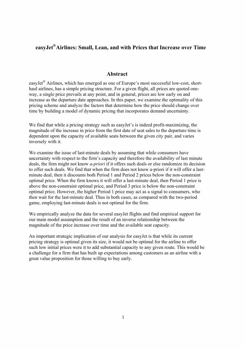
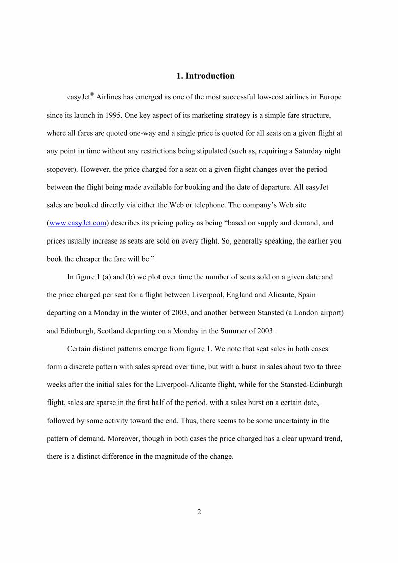
In figure 1 (a) and (b) we plot over time the number of seats sold on a given date and
the price charged per seat for a flight between Liverpool, England and Alicante, Spain
departing on a Monday in the winter of 2003, and another between Stansted (a London airport)
and Edinburgh, Scotland departing on a Monday in the Summer of 2003.
Certain distinct patterns emerge from figure 1. We note that seat sales in both cases
form a discrete pattern with sales spread over time, but with a burst in sales about two to three
weeks after the initial sales for the Liverpool-Alicante flight, while for the Stansted-Edinburgh
flight, sales are sparse in the first half of the period, with a sales burst on a certain date,
followed by some activity toward the end. Thus, there seems to be some uncertainty in the
pattern of demand. Moreover, though in both cases the price charged has a clear upward trend,
there is a distinct difference in the magnitude of the change.

3
Figure 1a: Seats sold and prices paid (in British pounds) of a one-way ticket from Liverpool to Alicante (flight date January 27, 2003)
0102030405060708090100
20/01/03
15/01/03
12/01/03
08/01/03
04/01/03
29/12/02
26/12/02
19/12/02
16/12/02
12/12/02
08/12/02
02/12/02
26/11/02
20/11/02
15/11/02
pric
e
0
20
40
60
80
100
120
140
160
seat
s
price seats
Figure 1b: Seats sold and prices paid (in British pounds) of one-way ticket from
Stansted to Edinburgh (flight date July 21, 2003)
0
10
20
30
40
50
60
70
80
90
100
21/07/03
18/07/03
14/07/03
11/07/03
08/07/03
04/07/03
01/07/03
26/06/03
17/06/03
12/06/03
03/06/03
03/05/03
22/04/03
27/03/03
21/02/03
pric
e
0
20
40
60
80
100
120
140
seat
s
price seats

4
For the Liverpool-Alicante flight, the price increases by about 2.5 times, from about £40 to
£100, whereas the price increase for the Stansted-Edinburgh flight is about 4.5 times, from
around £20 to a high of £90.
In this paper, we address the following issues relating to easyJet’s pricing strategy: How
should the airline price the seats over time? Is increasing price over time an optimal strategy?
How is the pricing strategy influenced by customer heterogeneity? What factors determine the
rate at which price increases over time? Does it pay to have last minute deals?
We develop a two-period analytical model of dynamic pricing and determine how
prices change over time, given i) the presence of two types of customers who value air travel
differently and ii) a level of airline seat capacity. A key factor in our model is the existence of
uncertainty in demand for one of the customer groups. We solve for the equilibrium two-
period prices in a game in which the airline maximizes profits and customers maximize utility.
We find that the equilibrium prices increase over time for all levels of capacity. In the
high-capacity case, the firm practices straightforward price discrimination between the two
segments. In the intermediate case, the firm adjusts the level of prices for both segments. That
is, it does not serve the business passenger first and use the tourists as a buffer in case it has
some excess capacity, but rather restricts the demand of both segments (by raising the
appropriate prices) so as to match capacity with expected demand. Only in the low-capacity
case does the firm forgo the tourist segment and serve the business segment exclusively.
We also find that when capacity is high, the prices in the two periods are independent of
the level of capacity, and thus the difference between the prices in the two periods is
independent of the level of capacity. When capacity is low or medium, the levels of prices do
5
depend on capacity. In addition, the difference between the two prices either remains constant
or decreases as capacity increases.
We examine the issue of last-minute deals by assuming that while consumers have
uncertainty with respect to the firm’s capacity and therefore the availability of last minute
deals, the firm might not know a-priori if it offers such deals or else randomize its decision to
offer such deals. We find that when the firm does not know a-priori whether it will offer a
last-minute deal, then it discounts both Period 1 and Period 2 prices below the non-constraint
(i.e. the results mentioned previously when last minute deals were not a consideration) optimal
price. When the firm knows it will offer a last-minute deal, then Period 1 price is above the
non-constraint optimal price, and Period 3 price is below the non-constraint optimal price.
However, the higher Period 1 price may act as a signal to consumers, who then wait for the
last-minute deal. Thus in both cases, as compared with the two-period game, employing last-
minute deals is not an equilibrium.
The empirical results support the main assumption in our model development that there
are heterogeneous groups of customers with differing price responses. The empirical results
also support the main results or predictions of our model that the seat price increases over
time, but the rate at which price increases declines as capacity increases, i.e., that there is an
inverse relationship between the rate at which price increases over time and the available seat
capacity. We further find that price at each point of time is a function of the remaining
capacity at that point of time.
The rest of this paper is organized as follows. In the next section, we relate our research
to the extant literature on airline pricing. In section 3, we lay out the structure of the model and
the underlying assumptions. This is followed by the derivation of our main analytical results in

6
section 4. We next consider in section 5 the special situation of last-minute deals. In section 6
we describe our empirical analysis to test the validity of the model’s main assumption and to
verify whether the prediction of the model of an inverse relationship between price increase
and seat capacity holds. In section 7, we conclude by summarizing our results and identifying
issues for future research.
2. Related Literature
Our work ties in to the research literature on airline pricing and to the yield
management literature. Yield management is a rich research area that has attracted the
interest of both operations management and economics researchers. McGill and van Ryzen
(1999) provide a detailed survey that reviews the work on yield (revenue) management.
They discuss four areas: forecasting, overbooking, seat inventory control, and pricing.
Traditionally, the operations literature on airline yield management concerns itself with
seat inventory and capacity planning problems (see, for example, Talluri and van Ryzen
2004; Lautenberg and Stidham 1999; and Belobaba 1987). However, there is also an
increasing body of research that considers pricing decisions, such as Talluri and van Ryzen
2004; You 1999; Feng and Gallego 1995; Gallego and van Ryzen 1997 and 1994; and
Watherford and Pfeifer 1992. In general, this branch of work focuses on dynamic pricing
decisions under a capacity constraint.
Feng and Gallego (1995) look at the optimal timing for changing prices, and show
that under mild conditions, it is optimal to decrease prices as flight time approaches.
Gallego and van Ryzen (1994) tie together the decisions of pricing and seat allocation and
show how price can be used as a tool to shift demand from one customer class to another.
7
In a recent book chapter, Talluri and van Ryzen (2004) write about the economics of
revenue management and focus on pricing decisions.
Our research also draws on the economics literature on airline pricing (see, for
examples, Dana 1998 and 1999; Kretsch 1995; Morrison and Winston 1990; Borenstein
and Rose 1994). Similar to our work, Dana (1999) looks at a market with two segments:
tourist and business. Dana assumes that tourist passengers are consumers with relatively
lower “waiting” costs, while business passengers are consumers with relatively higher
“waiting” costs, where the cost of waiting is a stochastic variable that defines the cost of
flying at the least desirable time. Dana assumes that there are two times to fly, that the
peak time can be either one with probability 0.5, and consumers’ preferences are perfectly
inversely correlated. Dana presents a stylized model that suggests that yield management
may be an efficient equilibrium response to uncertainty regarding the distribution of
consumers’ departure time preferences. Dana looks at both monopoly and competitive
equilibrium pricing and analyzes the firms’ optimal pricing decisions in each case. Dana
shows that under his model assumptions, an increase in the number of tourist passengers
actually serve to benefit business passengers. Tourists not only occupy a relative majority
of the low-priced seats; they also lower the prices for business passengers. Thus, Dana
shows that business passengers are better off with price discrimination.
Finally, our work relates to the marketing literature on pricing under conditions of
uncertainty in general and airline pricing in particular. Carpenter and Hanssens (1994) test
the optimality of an airline (UTA) pricing strategy and measure the impact of price on the
overall size of the market for air travel between Cote d’Ivoire and Paris. They find the
optimal prices under capacity constraint and forecast demand for these fares. Carpenter

8
and Hanssens provide a decision support system that finds the optimal prices, forecasts the
market response, and constructs a response model for total volume and fare class share.
Based on this analysis, they offer a forecasting model to estimate overall demand for each
fare class. Desiraju and Shugan (1999) find that yield management systems (like early
discounting, overbooking, and limiting early sales) for capacitated systems are optimal
when price-insensitive consumers choose to purchase later than price-sensitive consumers
do. Biyalogorsky et al. (1999) find that under some conditions, firms sell more units than
their capacity and then cancel (with appropriate compensation) sales made to consumers
who pay the list price. Biyalogorsky et al. show that this policy can actually improve both
profits and allocation efficiency. In another paper, Biyalogorsky et al. (2003) analyze
practices wherein consumers can choose from various service classes (e.g., airlines, hotels,
and rail transportation among others), each with limited capacity. They identify the
conditions under which the firms find it more profitable to upgrade services.
Another branch of work in marketing and economics that relates to our research is
that on advanced purchases (see, for examples, Shugan and Xie 2000; and Gale and
Holmes 1992, 1993). Shugan and Xie (2000) discuss the general role of advance pricing,
which is not necessarily unique to the airline industry. Under various conditions of
intermediary marginal costs, capacity constraint, seller credibility, and risk aversion, they
show that advanced selling is an optimal strategy if there is uncertainty on consumer-side
valuation. Xie and Shugan (2001), show that the additional profits come from the increase
in sales, but not from consumer surplus.

9
3. Model Development: Tourist and Business Segments
We consider a one-way airline route between two cities, with a monopoly service
provider. We assume there are two segments of customers (denoted T for tourists and B for
business) and two time-periods (denoted Periods 1 and 2). The tourists’ utility from the travel
is uniformly distributed over an interval of (0, α). This utility does not change over time and
thus in Period 2, their utility remains at exactly the same level as that of the previous period.
Business consumers arrive in both periods: A fraction γ of the business segment arrives
in period 1. Their utility from the travel is distributed uniformly over the interval of ),( αα . A
fraction (1- γ) of the business segment appears in Period 2. These consumers, however, have
uncertainty with respect to their utility. The business passenger learns during Period 2 that
with probability θ a business meeting that requires air travel is to be held at the destination
city. With probability (1 - θ), this business meeting is not held, and the utility of this executive
from the air travel thus equals zero. In order to create a clear-cut segmentation between
business and tourists, we assume that the upper bound of the valuation of the business
consumer is much higher that that of the tourist, i.e., 2/αα < .
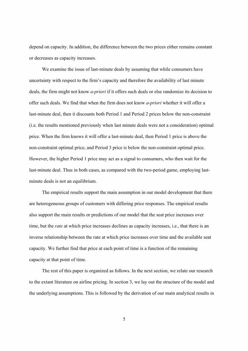
Assume there are two periods in which passengers can buy an air ticket. The sequence
of events is given in Figure 2 as follows:
Figure 2: Sequence of pre-flight events

10
There are two events in Period 1: first, the firm announces the price, and then consumers make
a decision whether to buy. There are three events in Period 2: first, the firm announces price.
Next, uncertainty about the state of the business passengers is resolved. Finally, consumers
make a decision whether to buy the ticket. Let f(x) be the density of consumer distribution. As
the tourist customers are distributed uniformly in the interval (0, α), the following
holds: ∫ =α
0
1)( dxxf . Thus f(x) = 1/α. If the price in Period 1 or 2 is p, then the tourists whose
utility is larger than the price will buy the tickets. Thus, the proportion of those who buys seats
in Period 1 at price p is represented by: ∫ −=α
ααp
pdxxf /)()( . Similarly, the proportion of
business passengers buying tickets at a price of p in Period 2 is represented by:
∫ −−=α
αααp
pdxxf )/()()(
If the number of tourist passengers is denoted by MT, and the number of business
passengers by MB, then their respective demands at a price of p are given by MT (α - p)/α,
and MB (_
α -p) / (_
α -α). In order to simplify notations, we normalize the market sizes as
follows: NT = MT /α and ΝΒ = MB / (_
α - α). We assume that MT > γNB and that NT > γ NB .
We shortly show (in section 4.3) that in the reverse case when γ NB >NT the problem is rather
trivial, as the firm would rather sell only to business consumers.
Customers will decide to purchase the ticket in period i (i = 1,2) if the utility in this
period will be positive and higher than the utility of purchasing in the other period. Therefore,
the following system represents demand in the two periods:

11
( ) ( )
>>−
<+−−=
αααγ
αγα
11
111 )(
1,1
pifpN
pifNpLNDperiod
B
BTT
( ) ( ) TTB LpNpNDperiod 222 )1(,2 −+−−= ααθγ
LT is an identity function that equals 1 if the tourist customer purchases the product in
Period 2, and zero if s/he purchases the product in Period 1. The condition LT = 1 is that the
Period 2 price is lower than the Period 1 price (we assume that there is no discounting factor
and that the consumer would rather buy today than wait if the prices in both periods are the
same). Thus LT are represented by:
<
=otherwise0
1 12 ppifLT
Without loss of generality, let the marginal cost of supplying the seat be zero. Let the
capacity (the number of airline seats) be fixed at C. Restrictions on capacity play a dominant
role in our analysis, as will be explained later on.
4. Derivation of Equilibrium Prices
From the assumptions specified in the previous section and from the demand system,
we can show that the firm should consider three cases. The first case is where capacity is so
low that the firm sells only to business consumers. The second case is where capacity is
binding but is high enough such that the firm can effectively discriminate, so that it sells to
both markets, while the third case is where capacity is high enough and is not effectively
binding. A concise summary and a graphical presentation of the pricing results are given in
Table 1 and Figure 3 at the end of this section. In order to set the boundary of these cases,
define β(C) to be:

12
CNNC BT −−+−+= 2/])1()([2/)( αθγααγαβ
We will shortly show (in section 4.3) that β(C) is the capacity shortage, i.e., the difference
between demand and capacity. Thus when β(C) > 0 indeed the firm faces capacity shortage
and when β(C) < 0, the firm has excess capacity.
4.1 Prices and profits with low capacity
When capacity is low, the firm is better off selling exclusively to business consumers,
who have higher valuation and thus will pay more. We will shortly show that this case could
be divided into two sub-sections: very low and low.
Consider the extreme case when the firm has only one seat available. Obviously, the
firm would rather sell it to a business consumer who has higher valuation. As we increase the
capacity, this policy is valid until capacity exceeds the optimal selling quantity to the business
segment 2/))1((1 θγθα −+= BNC . It is easy to show that the corresponding price is the
monopoly price, p = 2α . Equivalently, this case corresponds to a large capacity shortage,
i.e., 2/)()( BT NNC γαβ −> . Thus the following proposition holds for this low-capacity case
(for a proof see the appendix):
Proposition 1: With low capacity C < 1C optimal prices are given by:
))1((21 θγθα
−+−==
BNCpp . When 1C < C < 2C the firm charges 2/21 α== pp .
In order to find out the value of 2C , note that when the capacity equals 1C , the firm
charges the optimal monopoly price p = 2α and sells only to the business segment. When
the capacity increases further, the firm does not immediately decrease the price in the first

13
period order to capture more demand from the tourist segment and compensate by increasing
price in the second period to the business segment. The firm employs this policy only when
the additional revenues from the tourist segment compensates for the loss in revenues from the
business segment. Up to this capacity (defined as 2C ) the firm would keep the price constant at
p = 2α in both periods and serve only the business segment. We derive the value of 2C in
the appendix.
4.2 Prices and profits with intermediate capacity
One might have expected that when capacity increases further, the firm continues to
sell to the business consumers in the second period at price of p2 = 2α and starts to sell
to tourist consumers in the second period in a reduced price as fillers in order to increase
utilization. This however, is not the case. In this section we show that the optimal pricing
scheme is to increase the price over time so as to discriminate between the two segments
when the capacity is intermediate in value, 32 C CC << , where C3 is given by β(C3)=0.
Thus, this section deals with the case where there is capacity shortage, but it is not
exceedingly acute as in the previous case.
The overall optimization problem is represented by:
Period 2: ( )22 )1( pNpMax B −− αθγ
Subject to: ( ) ( ) ( ) 0)1( 21 >−−−−−−− pNNpNC BBT αγθααγα
Period 1: ( ) ( ) 211 ][ ∏+−+− ααγα BT NpNpMax
Subject to: ( ) ( ) ( ) 0)1( 21 >−−−−−−− pNNpNC BBT αγθααγα and α - p1 > 0

14
We define Lagrangian in Period 2 with coefficient λ, and in Period 1 with coefficients δ
and µ.
( ) ( ) ( ) ( )])1([)1( 21222 pNNpNCpNpL BBTB −−−−−−−+−−= αγθααγαλαθγ
( ) ( )( ) ( ) ( ) )(])1([
][
121
2111
ppNNpNCNpNpL
BBT
BT
−+−−−−−−−+∏+−+−=
αµαγθααγαδααγα
In order to find the sub-game perfect equilibrium, we solve the game backward
starting in Period 2, and find out the optimal prices as given in the following proposition:
Proposition 2: With intermediate capacity 2C < C < 3C , the optimal prices are represented by
BTT
B
NNC
NN
p)1(
)(2
)(21 γθ
βααγα−+
+−
+= and BT NN
Cp)1(
)(22 γθ
βα−+
+=
It is clear that the price in Period 2 in this case is also higher than the price of Period
1 since the inequality NT > γ NB holds. Thus, optimal prices are increasing over time. Note
that, because of the constraint on C, the term β is positive, and thus both prices are higher
than the monopoly unconstrained prices. In the next section we derive these latter prices.
4.3 Prices and profits with high capacity
Finally, we analyze the case where the capacity constraint is not binding. In this case we
follow the same route as the previous case, mutatis mutandis, to come up with:

15
Proposition 3: With excess capacity C > 3C , the optimal prices are represented by
T
B
NN
p2
)(21
ααγα −+= and p2 = 2α .
With these prices it is straightforward to compute the overall demand D to be:
2/])1()([2/ αθγααγα −+−+= BT NND . It is now clear that β(C) is indeed the
difference between demand and capacity (D-C), i.e. the capacity shortage.
It is also straightforward to see that p1 < p2 if (and only if) NT > γ NB. If this constraint
is not satisfied then the firm is better of charging p = 2α in both periods and serve only the
business segment. Since this latter case is almost trivial in its implications, we have assumed
throughout the paper that the tourist segment is larger that the business segment appearing in
the first period, i.e., NT > γ NB.
The optimal first- and second-period prices for each capacity scenario (low,
medium, and high) are summarized in Table 1 and Figure 3:
Table 1: (Perfect) equilibrium prices for varying levels of capacity
Capacity Period 1 price Period 2 price
Very low capacity (C < C1)
))1((1 θγθα
−+−=
B
vl
NCp
vlvl pp 12 =
Low capacity (C1 < C < C2)
21 α=lp
ll pp 12 =
Medium capacity (C2 < C < C3)
BT
hm
NNCpp
)1()(
11 γθβ
−++=
BT
hm
NNCpp
)1()(
22 γθβ
−++=
High capacity (C3 < C)
T
Bh
NN
p2
)(21
ααγα −+=
22 α=hp
Where β is the capacity shortage, i.e., ( ) CNNC BT −−+−+= 2/)1()(2/)( αθγααγαβ
16
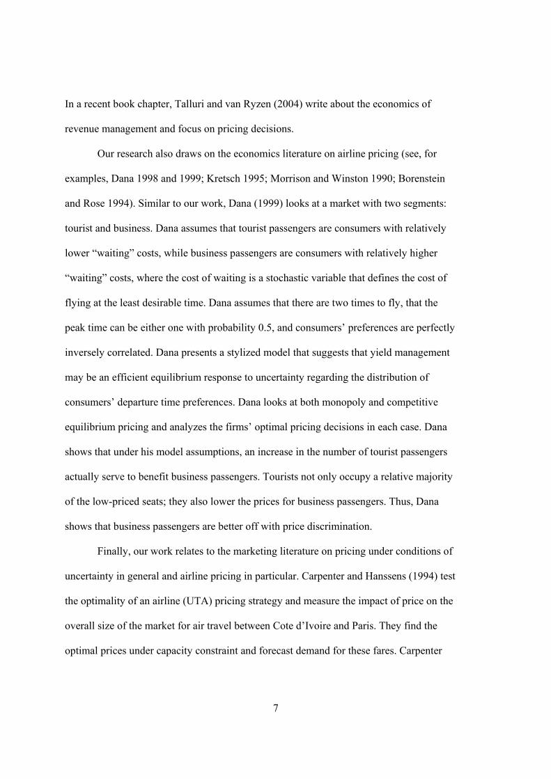
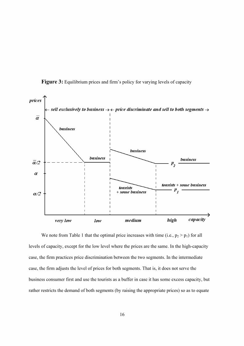
Figure 3: Equilibrium prices and firm’s policy for varying levels of capacity
We note from Table 1 that the optimal price increases with time (i.e., p2 > p1) for all
levels of capacity, except for the low level where the prices are the same. In the high-capacity
case, the firm practices price discrimination between the two segments. In the intermediate
case, the firm adjusts the level of prices for both segments. That is, it does not serve the
business consumer first and use the tourists as a buffer in case it has some excess capacity, but
rather restricts the demand of both segments (by raising the appropriate prices) so as to equate
17
capacity to expected demand. Only in the low-capacity case, does the firm forgo the tourist
segment and serve the business segment exclusively. We also note that when capacity is high,
the prices in the two periods are independent of the level of capacity, and thus the difference
between the prices in the two periods is independent of the level of capacity as well. When
capacity is low or medium, the levels of prices do depend on capacity.
If the capacity C is a strategic decision variable of the firm and it is costly, then the firm
would never choose levels of capacity such that 1C < C < 2C or C > 3C as in these capacity
regions, as capacity increases neither the price nor demand change and thus it pays more for
capacity while its revenues remain unchanged.
Further, in certain regions of the capacity, we confirm Dana’s result (1999) that the
tourist travelers subsidize the business consumers. Thus when 2C < C < 3C an increase in
capacity causes the number of tourists to increase and the price to the business consumers to
decrease. However, this is not the case when the capacity is at the point C2. At this point the
firm moves from selling only to the business consumers at a relatively low price of p = 2α to
price discriminating between the two segments by selling to the business at a much higher rate
and to tourist at a much lower rate. Thus at this capacity the business consumers suffer from
having the tourists join the flight as they pay a higher price.
5. Last-Minute Deals
In actual practice, we do observe last-minute deals that are often offered at a very low
price. If the firm decides to engage in such offers, either directly or via a reseller, then it can
set a new price so as to attract the lower end of the tourist segment that did not purchase the
18
tickets in the first period. What we show in this section is that either this policy is not optimal,
or it involves a time inconsistency problem on the part of consumers. In addition, if the time
inconsistency problem is solved, for example by introducing information asymmetry, then it is
clear that this policy is suitable for firms with high capacity. In other words, what we find is
that easyJet is behaving optimally in that it increases prices over time, and will continue to
behave optimally by increasing prices as long as it remains a small airline. Its policy might not
be optimal as soon as it stops being small and lean.
Last-minute deals are often made very close to the actual flight time. For example, in
some European airports, one can buy tickets at a greatly reduced price for same-day flights.
Thus in actual practice, as well as in our models, last-minute deals are rendered irrelevant for
the business segment. If the price in Period 3 (last-minute period) is low, then the firm has to
worry about consumers from the tourist segment waiting to buy tickets in Period 3 instead of
buying them in Period 1. Indeed, some of them will, but the question is how to fence the
higher utility consumers out of this segment. The reason that the high-utility consumers do not
wait for last-minute deals is their uncertainty with respect to the existence of such deals. They
know that if demand is high enough, the airline will not bother reducing the price. Moreover,
if capacity is low relative to demand, then by waiting, they take the risk of finding themselves
without a ticket.
First, in order to simplify our three stage model we assume that the business consumers
appear only in the second period and thus γ = 0. We model the uncertainty of the consumers
with respect to the capacity with the help of an additional parameter β. With probability β,
capacity is high and the airline offers last-minute deals, and if capacity is low, then with
probability (1-β) it does not. In what follows, we offer two possible options on the part of the
19
airline: It can either randomize with respect to last-minute deals, or it knows with certainty
whether it will engage in such practice. As we will see, the option chosen does have an effect
on the optimal prices, and consequently on the behavior of the consumers.
Let x be the tourist with the highest utility that will purchase the ticket in Period 3 at the
price of p3. What we do next is to find the values of x, p1, p2, and p3 that will constitute an
equilibrium to the new game. We begin at Period 3 where the profits are represented by:
απ /)( 333 ppxM T −=
Maximization with respect to the price yields that
p3 = x/2, and α
π4
2
3xM T= .
In Period 2, the expected profits depend on the business segment and the expected
Period 3 profits. We define δ as an indicator parameter that is equal to 1 if the firm decision
whether to introduce Period 3 prices is unknown to the firm prior to Period 3, and that δ is
equal to 1/β if the firm knows with certainty that it will provide a ‘’last-minute deal.’’ Thus,
Period 2 profits can be represented as:
322
2)(
δβπαααθ
π +−
−=
pMp B
First-order conditions imply that the price in Period 2 is represented by:
p2 = _
α /2, and the profits are represented by α
δβαααθ
π4)(4
22
2xMM TB +
−= .
In Period 1, profits are represented by:
αδβ
αααθ
αα
π4)(4
)( 221
1xMMxpM TBT +
−+
−= .

20
We now use the fact that x is the marginal consumer for whom the utility from purchasing the
ticket in Period 1 is exactly equal to the utility from waiting and buying the ticket in Period 3.
This fact yields the following equation for x:
x – p1 =β (x – p3 ).
Substituting p3 = x/2 and solving for x yield:
β−=
22 1px
Substitute this expression for x in the profit function π1 yield:
2
21
211
1 )2()(4)
22
(βα
δβαααθ
βα
απ
−+
−+
−−=
pMMppM TBT
When the firm does not know if it will introduce a last-minute deal (δ =1), the first-order
condition for optimality yields the following solution for p1: )34(2
)2( 2
1 ββα
−−
=ap and
)34(2)2(
3 ββα
−−
=ap . It is easy to see that ap1 >ap3 and that ap1 < 2
α as 03422
2
1 <−
−=−
βββααap .
When the firm knows that it will introduce a last-minute deal (δ =1/β), the first-order condition
for optimality yields the following solution for p1: )23(2)2( 2
1 ββα
−−
=bp and )23(2)2(
3 ββα
−−
=bp . It is
easy to see that bp1 >bp3 and that bp1 > 2
α , as 023
)1(22
2
1 >−−
=−β
βααbp .
Proposition 4: a. When the firm does not know whether it will offer a last-minute deal (δ =1), then it discounts both Period 1 and Period 3 prices below the non-constraint optimal price, i.e., α/2> ap1 >
ap3 . In this case, as compared with the two-period game, employing last-minute deals is not optimal for the firm. b) When the firm knows it will offer a last-minute deal (δ =1/β), then Period 1 price is above the non-constraint optimal price, and Period 3 price is below the non-constraint optimal price, that is: bp1 >α/2>
bp3 .
21
With incomplete but symmetric information (Proposition 4a), when the firm offers a
last-minute deal, it charges the tourist consumers two discrete prices, both of which are below
α/2. Note from Table 1 that with γ = 0, 2/1 α=hp and thus these two prices are lower than the
optimal price for the tourist segment. Therefore, the firm sells to more consumers in the tourist
segment and generates lower-than-optimal profits. The reason for this sub-optimal behavior is
the commitment to a price reduction in Period 3. When such a commitment is made, some
strategic consumers with marginal valuations above price would choose to wait to obtain the
ticket at a lower price, thereby forcing the firm to reduce prices further in Period 1.
With asymmetric information (Proposition 4b), the optimal policy is to offer last minute
deal. The reason that it is indeed optimal is that the firm succeeds in discriminating between
two classes within the tourist segment, based on their valuation. This discrimination, however,
is possible only under the existence of uncertainty of consumers. Those with high valuation
will not care to wait for the super last minute deal as they have uncertainty with respect to the
capacity of the firm. The low valuation tourist will indeed wait, knowing that the flight might
be sold out, and buy at the last minute if tickets are still available.
There are cases under which this uncertainty is resolved, and thus this policy break
down. We next discuss two such cases. In this paper, we model a single flight. In this case,
this policy of offering last minute deal is optimal. However, in case that the game is repeated
and the consumers update their expectation, the consecutive appearance of last minute deals
will resolve their uncertainty. In this case, when β=0, all tourist consumers will wait and
purchase tickets at the last minute. In addition, suppose that consumers can compare the last
minute deal policy to a two periods policy (with out a last minute deal). In this case the fact

22
that the first period price is above α/2, removes uncertainty and consumers will wait and
purchase tickets at the last minute.
One can ask the question whether the airline should price to sell all the remaining seats
in period 3. The answer clearly depends on the capacity. Proposition 4b was solved under the
assumption of unconstraint capacity. The demand of this case can be shown to be
.)23(2
)34(2 β
βαα−
−+= TB NND The firm will sell all the remaining seats if (and only if) the
capacity is lower than this demand, D.
We base our analysis on the assumption of two segments that differ in their valuations
over-time. We find that the firm’s optimal policy under these assumptions is to charge a
relatively low price in Period 1, and to increase the price in Period 2, and not to offer a period
3 price. If the firm decision regarding whether to offer the service in period 3 or not is
exogenous, then the firm decreases the price below the first period price. We further show that
this price change is a function of seating capacity.
At first glance our result appears to differ from some previous findings (for example
Xie and Shugan 2001). They find that under high (but not unlimited) capacity, advance (high)
pricing at a premium to the spot price is an optimal strategy, and that the firm generates more
revenues from the increased demand (consumers buy at a price that equals their expected
value and that may exceed their true value).
There are two major assumptions in the models that derive this difference. First, Shugan
and Xie assume that consumers in each of the two market segments have the same valuation
for the service. Our work, however, assumes that each segment has its own continuous
distribution function for the valuation of the product, which may change over time. Second,
we assume that the business segment has clearly higher future valuation and therefore, the firm

23
finds it optimal to charge non-decreasing prices. In the next section, we show empirically that
our assumption that there are two segments in the market is consistent with the easyJet market
and that prices are changed as a function of capacity.
6. Empirical Analysis
For our empirical analysis, we have data on 23 easyJet flights between six different
European city pairs during the year 20031. Some of these flights are in the winter and others in
the summer. The flights depart on two different days of the week – Monday and Sunday. For
each flight we have data from the first day on which the seats were available to the traveling
public up to the date of departure. The duration ranged from 63 days for a flight between
Liverpool, England and Alicante, Spain to a maximum of 211 days for a flight between East
Midlands, England and Barcelona, Spain. For each flight, we also have data on the number of
seats sold per day (if any) and the price at which each was sold. Additionally, we also have
data on the total available easyJet seat capacity between each city pair.
The first phase of analysis is to test the validity of the assumption that there exist two
segments (and possibly a third segment in the case of last-minute deals) of customers with
differing price responses. Since the data suggest that customers arrive at discrete points in time
(see figure 1), a latent class Poisson regression model would be an appropriate way to model
that, see Wedel et al. (1993).2
1 Data pertaining to one flight had to be deleted, resulting in 23 usable observations. 2 The Negative Binomial (NB) distribution has also been used in previous research to model the aggregate demand for airline seats as it overcomes some of the well-known limitations of a Poisson model. We note that an aggregate NB model for demand can be derived by assuming that demand is Poisson at the individual level and accounting for heterogeneity over individuals using a gamma distribution. In our analysis, we model demand at the individual level using a Poisson model, but account for heterogeneity using a latent class approach, which can be also interpreted as providing a finite approximation to any mixing distribution, such as the gamma. Therefore, the demand model we use is quite flexible.
24
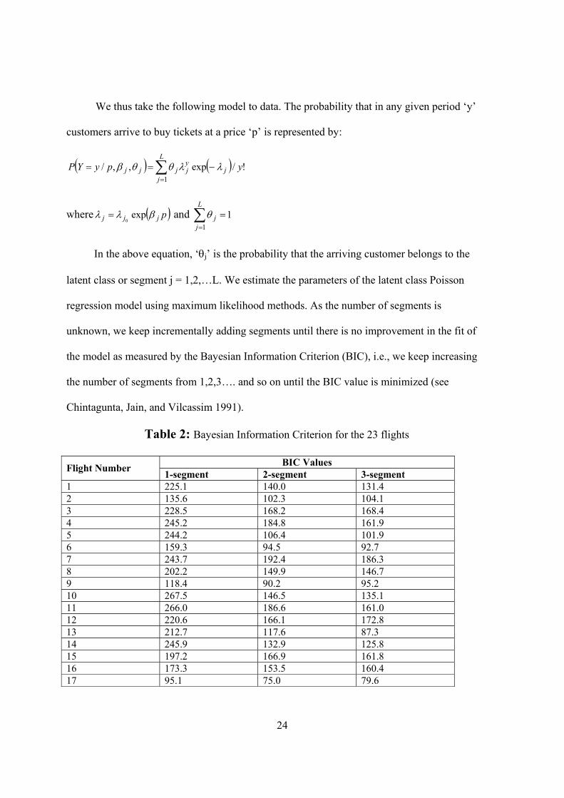
We thus take the following model to data. The probability that in any given period ‘y’
customers arrive to buy tickets at a price ‘p’ is represented by:
( ) ( ) !/exp,,/1
ypyYP jyj
L
jjjj λλθθβ −== ∑
=
where ( )pjjj βλλ exp0
= and ∑=
=L
jj
11θ
In the above equation, ‘θj’ is the probability that the arriving customer belongs to the
latent class or segment j = 1,2,…L. We estimate the parameters of the latent class Poisson
regression model using maximum likelihood methods. As the number of segments is
unknown, we keep incrementally adding segments until there is no improvement in the fit of
the model as measured by the Bayesian Information Criterion (BIC), i.e., we keep increasing
the number of segments from 1,2,3…. and so on until the BIC value is minimized (see
Chintagunta, Jain, and Vilcassim 1991).
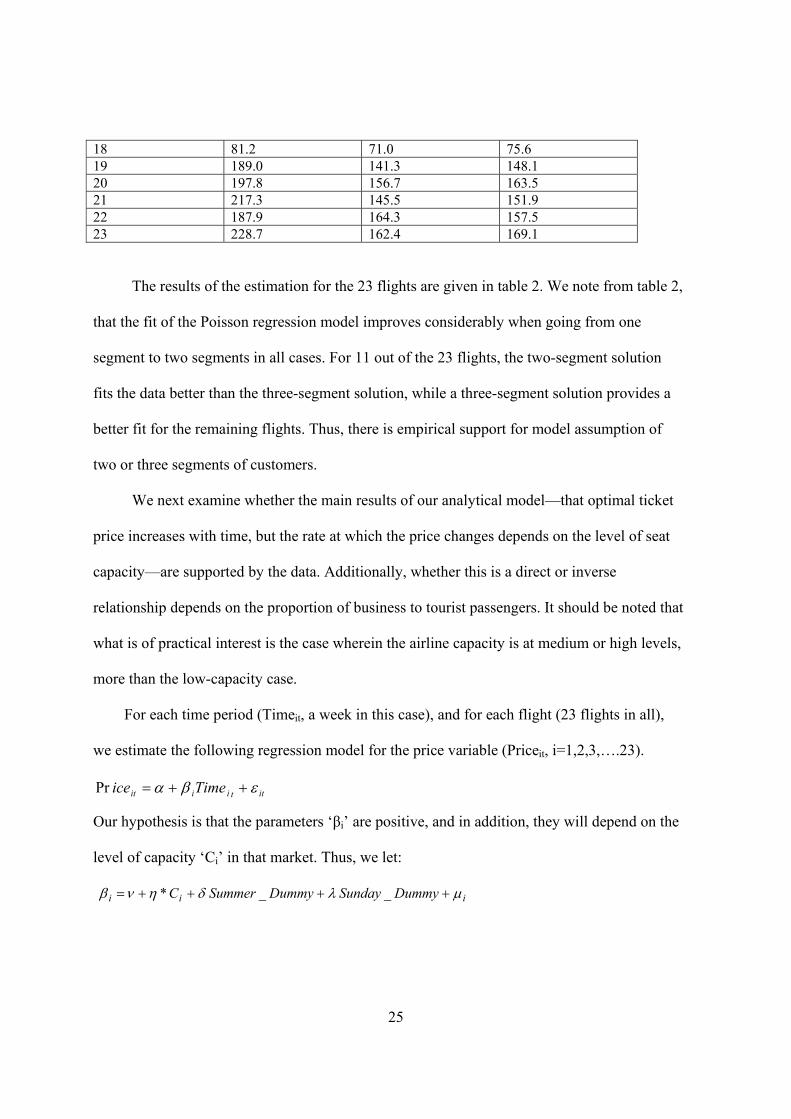
Table 2: Bayesian Information Criterion for the 23 flights
BIC Values Flight Number 1-segment 2-segment 3-segment 1 225.1 140.0 131.4 2 135.6 102.3 104.1 3 228.5 168.2 168.4 4 245.2 184.8 161.9 5 244.2 106.4 101.9 6 159.3 94.5 92.7 7 243.7 192.4 186.3 8 202.2 149.9 146.7 9 118.4 90.2 95.2 10 267.5 146.5 135.1 11 266.0 186.6 161.0 12 220.6 166.1 172.8 13 212.7 117.6 87.3 14 245.9 132.9 125.8 15 197.2 166.9 161.8 16 173.3 153.5 160.4 17 95.1 75.0 79.6
25
18 81.2 71.0 75.6 19 189.0 141.3 148.1 20 197.8 156.7 163.5 21 217.3 145.5 151.9 22 187.9 164.3 157.5 23 228.7 162.4 169.1
The results of the estimation for the 23 flights are given in table 2. We note from table 2,
that the fit of the Poisson regression model improves considerably when going from one
segment to two segments in all cases. For 11 out of the 23 flights, the two-segment solution
fits the data better than the three-segment solution, while a three-segment solution provides a
better fit for the remaining flights. Thus, there is empirical support for model assumption of
two or three segments of customers.
We next examine whether the main results of our analytical model—that optimal ticket
price increases with time, but the rate at which the price changes depends on the level of seat
capacity—are supported by the data. Additionally, whether this is a direct or inverse
relationship depends on the proportion of business to tourist passengers. It should be noted that
what is of practical interest is the case wherein the airline capacity is at medium or high levels,
more than the low-capacity case.
For each time period (Timeit, a week in this case), and for each flight (23 flights in all),
we estimate the following regression model for the price variable (Priceit, i=1,2,3,….23).
Our hypothesis is that the parameters ‘βi’ are positive, and in addition, they will depend on the
level of capacity ‘Ci’ in that market. Thus, we let:
iii DummySundayDummySummerC µλδηνβ ++++= __*
ittiiit Timeice εβα ++=Pr

26
where Summer_Dummy = {1 if the flight is in the summer, and 0 in the winter} and
Sunday_Dummy = {1 if the flight is on a Sunday and 0 on Monday}are two control variables
that we introduce because they could affect the rate at which price changes.
Table 3: Regression results - price vs. capacity
The results of the regression are given in table 3. We see from table 3 that in the
Price vs. Time regression, 20 out of the 23 slope coefficients (βi) are positive, and their
Regression Analysis Price-Time Regression Price Slope - Capacity Regression
Flight # Price Slope (β) Variable Estimate (standard error)
1 0.856 Intercept 6.597 2 0.485 (2.569) 3 1.799 4 1.382 Capacity -4.058 5 0.203 (1.967) 6 0.426 7 0.821 Summer_Dummy -1.148 8 0.492 (0.623) 9 0.780 10 -0.302 Sunday_Dummy 0.051 11 0.542 (0.617) 12 0.485 13 2.497 R-Square 25.8% 14 0.267 15 0.645 16 1.293 17 5.430 18 5.618 19 -1.031 20 -0.564 21 0.706 22 0.889 23 0.679
Mean Slope 1.061
27
overall mean is positive (1.061). This supports our result that the optimal prices increase
over time. We also note from table 3 that the coefficient of the capacity variable is
significantly different from zero, implying, as per our analytical model, that we are dealing
with the situation of intermediate capacity. This result is certainly reasonable for an airline
like easyJet, as opposed to say, British Airways, which can be considered to have high
capacity. When we examine the sign of the coefficient of the capacity variable, it is
negative, implying that as capacity increases, the rate at which price changes decreases.
Another way to look at the relationship between price and capacity is to regress price
against remaining capacity. Recall from the maximization problem for the intermediate
capacity case (section 4.2) that in Period 2, the firm maximizes profits subject to the
remaining capacity constraint and the main result was that the price is a declining function
of the remaining capacity (see Table 1). Therefore, for each time period (Timejt, a week in
this case), and for each pair of cities (six pairs), we estimate the following six regression
models for each city pair (four flights per city for five city pairs, and three flights per city
pair for a single flight for the remaining capacity variable (RemCapjt, j=1,2, ….J).
Our hypothesis is that the parameters ‘ jγ ’ are negative.
jtjtjjt DummySundayDummySummermCapice ξλδγα ++++= __RePr

28
Table 4: Regression results: price vs. remaining capacity
Route No. of flights
γ - Effect of remaining capacity
on price (standard error)
R Square
London (Stansted) – Edinburgh
4 -0.316 (0.026)
75.4%
East Midlands - Edinburgh
4 -0.155 (0.011)
74.6%
London (Stansted) - Rome (Ciampino)
4 -0.128 (0.023)
85.8%
East Midlands - Barcelona
4 -0.25 (0.029)
87.7%
Liverpool - Alicante
4 -0.137 (0.098)
65.2%
London (Luton) - Malaga
3 -0.145 (0.041)
49.6%
The results of the regression are given in table 4. We see from table 4 that in the
price vs. remaining capacity, all of the slope coefficients ( jγ ) are negative with an overall
mean of -0.189. This supports our result that the optimal prices decrease with the
remaining capacity.
Overall therefore, the empirical evidence is consistent with our main analytical
results on how optimal price varies with time, and how the change in price from one period
to another varies with the level of capacity.
7. Conclusions and Extensions
In this paper we have shown that the pricing strategy of easyJet that starts with a low
per-seat price and then increases it over time up to the time of departure is indeed an optimal
strategy. In addition, we showed analytically that the change in price depends on the airline’s
overall seat capacity between the given city pair.
29
We were able to support the findings of our analytical model with an empirical analysis
of several easyJet flight data. We showed empirically that the assumption of the existence of
two segments is consistent with the data, as is the main prediction that as capacity increases,
the change in price over time decreases. In other words, the greater capacity, the larger the pre-
ordering discount will be. We further find that price at each point of time is a function of the
remaining capacity at that point of time.
We also examined the phenomenon of last minute discounting by introducing a third
period into the analysis in which the firm finds itself with unsold seats. What we found is that,
as compared with the two-period game, employing last-minute deals is not optimal for the firm
due to time consistency issues and consumers’ rationality. However, in practice we observe
last minute deals. One explanation might be consumers’ difficulties in understanding the price
signals. An alternative explanation could be the myopic nature of the firm’s decisions makers.
A direct implication of our results is the following. We have shown that when the
airline prices (or permits resellers to price) last-minute deals, it should heavily discount pre-
orders, and this discounting should be heavier than the case in which the firm does not allow
for last-minute seat-clearing pricing. As shown in the examples and the empirical section,
easyJet’s pre-order discount is quite deep: A ticket that sells at less than £20 (about $30) two
months before the flight jumps to £130 (about $200) a couple of days before the flight.
However, large airlines that allow for last-minute clearing prices do not employ such
deep pre-order discounts (for example, one does not observe such deep discounting with an
airline like British Airways). Our results suggest that these “flat” pricing schemes, coupled
with last-minute deals, are not optimal. Thus, a key strategic issue for an airline like easyJet is
that were it to grow and add capacity to any route and become like a “large airline”, the firm

30
should avoid the temptation to offer last minute deals. easyJet has become successful precisely
by developing a strong value proposition among customers that translates into “I can get a
great deal by buying seats early on.” If changing that perception turns out to be a challenge,
then it may be prudent for easyJet to be extremely cautious about adding capacity on any
given route.
An interesting route to extend our study is the impact of competition on easyJet’s
dynamic pricing strategy. Some other airlines (for example, Ryanair3) also operate as low-cost,
short-haul carriers with similarly low prices offered early on to customers, while at the same
time long-haul flag carriers such as British Airways also have short-haul flights, but with
different pricing arrangements. Knowing whether the two-tiered pricing arrangements can be
sustained in such a competitive equilibrium is potentially an interesting research question with
important policy implications.
To summarize, our analysis has shed some interesting insights into the pricing strategy
of one Europe’s most successful low-cost, short-haul airlines. The pricing scheme used by
easyJet of starting with very low prices and then increasing them over time is indeed optimal,
and exploits heterogeneity in customer price sensitivity, given easyJet’s current size in the
European market. Were easyJet to grow and become larger, then its current strategy might no
longer be optimal. This poses an interesting challenge for the airline of whether to retain its
current size and strong value proposition, or become a larger airline with a new value
proposition that the market may not readily accept.
3 Recently Ryanair reported large losses which were attributed to its expansion that was much faster than easyJet’s cautious expansion (Done, 2004)

31
References
Belobaba, P. P. (1987), “Airline Yield Management: An Overview of Seat Inventory Control,” Transportation Science, (21), pp. 63-73.
Biyalogorsky, E., Carmon, Z., Fruchter, G. and Gerstner, E. (1999), “Overselling and Opportunistic Cancellations,” Marketing Science, (18), pp. 605-610.
Biyalogorsky, E., Gerstner, E., Weiss, D. and Xie, J. (2003), “The Economics of Service Upgrades,” working paper, University of California at Davis.
Borenstein, S. and Rose, L. R. (1994), “Competition and Price Dispersion in the US Airline Industry,” Journal Political Economy, (102), pp. 653-683.
Carpenter, G. S. and Hanssens, D. M. (1994), “Market Expansion, Cannibalization, and International Airline Pricing Strategy,” International Journal of Forecasting, (10), pp. 313-326.
Chintagunta, P.K, Dipak, C. Jain and Naufel, J. Vilcassim (1991), “Investigating Heterogeneity in Brand Preferences in Logit Models for Panel Data,” Journal of Marketing Research, 28, 99.417-428.
Dana, J.D. (1999), “Using Yield Management to Shift Demand When the Peak Time is Unknown,” Rand Journal of Economics, pp. 456-474.
Dana, J.D. (1998), “Advance-Purchase Discounts and Price Discrimination in Competitive Markets,” Journal of Political Economy, (106), pp. 395-422.
Desiraju, R. and Shugan, S. (1999), “Strategic Service Pricing and Yield Management,” Journal of Marketing, (63), pp. 44-56.
Done, K. (2004), “Ryanair’s dream run comes to an end,” Financial Times, January 29th.
Feng Y. and Gallego, G. (1995), “Optimal Starting Times for End-of-Season Sales and Optimal Stopping Times for Promotional Fares,” Management Science, (41), pp. 1371-1391.
Gale, I.L. and Holmes, T.J. (1992), “The Efficiency of Advance-Purchase Discounts in the Presences of Aggregate Demand Uncertainty,” International Journal of Industrial Engineering, (10), pp. 413-437.
Gale, I.L. and Holmes, T.J. (1993), “Advance-Purchase Discounts and Monopoly Allocation of Capacity,” American Economic Review, pp. 135-146.
Gallego, G. and van Ryzen, G. J. (1994), “Optimal Dynamic Pricing of Inventories with Stochastic Demand Over Finite Horizons,” Management Science, (40), pp. 999-1020.
Gallego, G. and van Ryzen, G. J. (1997), “A Multi-Product Dynamic Pricing Problem and its Applications to Network Yield Management,” Operations Research, (45), pp. 24-41.
Kretsch, S.S. (1995), “Airline Fare Management and Policy,” in The Handbook of Airline Economics, pp. 477-482.

32
Lautenberg, C.J. and Stidham, S.J. (1999), “The Underlying Markov Decision Process in a Single-Leg Airline Yield Management Problem,” Transportation Science, (33), pp. 136-146.
McGill, J. I. and van Ryzen, G. J. (1999), “Revenue Management: Research Overview and Prospects,” Transportation Science, (33), pp. 233-256.
Morrison, S.A. and Winston, C. (1990), “The Dynamics of Airline Pricing and Competition,” American Economic Review, (80), pp. 389-393.
Shugan, S. and Xie, J. (2000), “Advance Pricing of Services and Other Implications of Separating Purchase and Consumption,” Journal of Service Research, (2), pp. 227-239.
Talluri, K. and van Ryzen, G. J. (2004), The Theory and Practice of Revenue Management, Kluwer Academic Publishers, forthcoming.
Watherford, L.R. and Pfeifer, P.E. (1994), “The Economic Value of Using Advance Booking of Orders,” Omega, (22), pp. 105-111.
Wedel, M., Desabro, W.S., Bult, J.R. and Ramaswamy, V. (1993), “A Latent Class Poisson Regression Model For Heterogeneous Count Data,” Journal of Applied Econometrics, Vol. 8 397-411.
Xie, J. and Shugan, S. (2001), “Electronic Tickets, Smart Cards, and Online Prepayments: When and How to Advance Sell,” Marketing Science, (20), pp. 219-243.
You, P.S. (1999), “Dynamic Pricing in Airline Seat Management for Flights with Multiple Legs,” Transportation Science, (33), pp. 192-206.

33
Appendix: Proof of Propositions 1 and 2
The general optimization problem is represented by:
Period 2: ( )22 )1( pNpMax B −− αθγ
Subject to: ( ) ( ) ( ) 0)1( 21 >−−−−−−− pNNpNC BBT αγθααγα
Period 1: ( ) ( ) 211 ][ ∏+−+− ααγα BT NpNpMax
Subject to: ( ) ( ) ( ) 0)1( 21 >−−−−−−− pNNpNC BBT αγθααγα and α - p1 > 0
Thus we can define Lagrangian in Period 2 with coefficient λ, and in Period 1 with
coefficients δ and µ.
( ) ( ) ( ) ( )])1([)1( 21222 pNNpNCpNpL BBTB −−−−−−−+−−= αγθααγαλαθγ
( ) ( )( ) ( ) ( ) )(])1([
][
121
2111
ppNNpNCNpNpL
BBT
BT
−+−−−−−−−+∏+−+−=
αµαγθααγαδααγα
In order to find the sub-game perfect equilibrium, we solve the game backwards:
( ) 0)1(2)1( 222 =−+−−=∂∂ BB NpNpL θγλαθγ
Since in this intermediate case the constraint is binding, then 0>λ and thus
( ) ( ) ( ) 0)1( 21 =−−−−−−− pNNpNC BBT αγθααγα
Therefore the price is represented by:
( ))1(
)( 12 γθ
ααγαα−
−−+−+=
B
BT
NCNpNp
Substituting this price into the Lagrangian of Period 1 yields the following:
( )( ) ( ) )(
)1(])1()(][)([
)]([
111
111
pN
CNNpNCNpNNpNpL
B
BBTBT
BT
−+−
−−+−+−−−+−−−+−=
αµγθ
αθγααγαααγαααγα
Differentiating the Lagrangian with respect to p1 and equating to zero yields the optimal
solution for p1. It is straightforward to check that if ))1((2
θγθα−+> BNC , then α - p1 > 0,
thus µ = 0, and the optimal price in the first period is represented by:
BTT
B
NNC
NN
p)1(
)(2
)(21 γθ
βααγα−+
+−
+= ,
where β(C) is the capacity shortage, i.e., CNNC BT −−+−+= 2/])1()([2/)( αθγααγαβ .

34
Substituting this expression into the equation for p2 yields: BT NN
Cp)1(
)(22 γθ
βα−+
+= .
If, however, 2/))1(( αθγθ −+= BNC , then µ > 0, and the constraint is binding, i.e., α - p1 =
0. It follows that α≥1p . Substituting this expression into the expression for p2 yields the
following optimal second price period for the low capacity case: ))1((2 θγθ
α−+
−=BN
Cp .
Note that when 2/))1(( αθγθ −+= BNC , the firm sells to all the business consumers at
price 2/2 α=p . This generates the optimal unconstraint profits from the business segment.
However, when the capacity exceeds that threshold, the firm continues to charge the
competitive business price 2/2 α=p until capacity is large enough such that the benefit
revenues from the additional tourist consumers exceeds the loss from deviating from the
optimal price for the business consumers segment.
The loss in selling to the business consumers is given by:
.)()1()()]1([ 2211mm
Bm
BBl ppNpNNp −−−−−−+ αθγααγγθγ
The revenues from selling to the tourist segment are given by: ).( 11m
Tm pNp −α
Equating these two equation yields the threshold capacity level:
,2
)]]1(][)()[([])([ 22
2T
BTBTBTTBTT
NNNNNNNNNNN
Cγθααγαγγαγθθγαα −+−−−−−−++
=
such that for any 2])1([2
CCN B <<−+ θγθα , the firm charges 221α
== pp and for any
CC <2 the firm charges BTT
B
NNC
NN
p)1(
)(2
)(21 γθ
βααγα−+
+−
+= and
BT NNCp
)1()(
22 γθβα
−++= . Note, that 22/])1()([2/ CNN BT >−+−+ αθγααγα for
22 )( ααγα −≥ BT NN and that 2])1([2
CN B <−+ θγθα when
.02
)]]1(][)()[([ 222
>−+−−−+−
T
BTBTBTTTBT
NNNNNNNNNNN γθααγαγαγα If this condition is
not satisfied the firm moves directly from policy of low capacity to policy of intermediary
capacity.