eastern journal of european studies volume 10 issue 1 2019

EASTERN JOURNAL OF EUROPEAN STUDIES Volume 12, Issue 1, June 2021 5

DOI: 10.47743/ejes-2021-0101

Investigating the impact of GDP and distance

variables in the gravity model using sign and rank

tests

Berislav ŽMUK*, Hrvoje JOŠIĆ**

Abstract

The gravity model of trade has been a workhorse of international economics over

the last fifty years. The main variables incorporated in the standard gravity model

of trade are gross domestic product of trading countries and distance between them.

The previous investigation has been limited only to an econometric estimation and

evaluation of regression coefficients in the gravity model and their significance.

However, until now there has been no research on investigating the impact of GDP

and Distance variables in the gravity model by using sign and rank tests, which is

the objective of this paper. This paper adds to the existing literature by employing

non-parametric approach to estimating the impact of variables in the gravity model

by using sign and rank tests in the case of World countries. The results of the analysis

have shown that the GDP variable exhibits a higher distribution of positive signs

achieved in the sign test and presents less average errors in the rank test in

predicting bilateral trade imports with regards to the Distance variable.

Furthermore, the GDP variable also has a relatively higher impact in the gravity

model than the Distance variable.

Keywords: gravity model, World countries, sign and rank tests, RMSE, MAPE

Introduction

The gravity model has been firstly applied in the field of international trade in

1962 by Jan Tinbergen (Tinbergen, 1962) but the origins of the gravity model go

back to 1687 and the formulation of law of universal gravity developed by Isaac

Newton. The law of universal gravity states that the gravitational force between two

bodies is proportional to their masses and inversely proportional to the square of

distance between them. The gravity model in international economics puts this

*Berislav ŽMUK is Assistant Professor at the Faculty of Economics and Business in Zagreb,

Zagreb, Croatia; e-mail: [email protected]. **Hrvoje JOŠIĆ is Assistant Professor at the Faculty of Economics and Business in Zagreb,

Zagreb, Croatia; e-mail: [email protected].

6 | Berislav ŽMUK, Hrvoje JOŠIĆ

Eastern Journal of European Studies | 12(1) 2021 | 2068-651X (print) | 2068-633 (on-line) | CC BY | ejes.uaic.ro

relation into an economic context (Starck, 2012). The variable which usually

represents country’s economic size in the empirical literature is the gross domestic

product (GDP) while the distance between countries is most often approximated with

the aerial distance between countries’ capital cities. The gravity model is used to

correctly approximate bilateral trade flows and has long been one of the most

successful and stable empirical models in economics (Salvatici, 2013).

McCallum (1995) proved that national borders matter in the case of Canada's

intra-province trade being 23 times more intense than the trade between Canada and

the United States. Prior to the general acceptance of the gravity model, there have

been several criticisms related to its not having or lacking a strong theoretical basis,

Kareem and Kareem (2014). Nevertheless, the theoretical foundation of the gravity

model can be found in the work of Anderson (1979), Bergstrand (1985), Eaton and

Kortum (2002), Anderson and van Wincoop (2003), Helpman et al. (2008), etc.

The previous investigation of the gravity model has been limited only to

econometric specifications and the evaluation of regression coefficients in the

gravity model and its significance. However, until now there has been no research

related to the investigation of the variables’ impact in the gravity model, which is the

aim of this paper. The impact of GDP and Distance variables in the gravity model

will be evaluated by calculation and analysis of positive (correct) signs achieved in

the sign test and average errors between expected and actual ranks in the rank test.

Therefore, this paper adds to the existing economic literature in this field of research

by employing non-parametric approach to the estimation of the impact of GDP and

distance variables in the gravity model by employing the sign and rank tests. This is

a new idea using an old concept; the sign and rank tests are well known instruments

for testing the Heckscher-Ohlin theory (Ohlin, 1933) and the Heckscher-Ohlin-

Vanek theorem specifically (Vanek, 1968; Kohler, 1991).

The sign test displays the percentage of cases in which a certain variable has

been correct in predicting bilateral trade flows, in this paper imports, as the percent

of distribution of positive signs. The sign test for the GDP variable will be calculated

by comparing the difference between the actual GDP value of the import trade

partner country and the average GDP value (the arithmetic mean of values for all

import trade partner countries) with the difference between the actual imports value

and the average imports value. If, for example, the actual value of GDP of the import

trade partner country is higher than the average value, than the actual import value

should be higher than the average import value. In that case the positive sign will be

achieved in the sign test. The percentage of correct signs achieved in the sign test

should be higher than 50% in order in order for the results to make sense, otherwise

it becomes arbitrary and random. There are no defined certain thresholds in

economic theory for the sign test to be valid in verifying a hypothesis. However, a

higher percentage achieved in the sign test should support the hypothesis of the

paper. On the other hand, the rank test, using the root mean square error (RMSA)

Investigating the impact of GDP and distance variables in the gravity model | 7


and the mean absolute percentage error (MAPE), displays average errors between

expected and actual ranks.

Analysis will be conducted for all World countries for which data were

available. After that, the subsamples of countries will be analysed (CEE and EU

countries) as well as Croatia as an individual country from Central and Eastern

Europe having membership in the EU. It is expected that GDP and Distance variables

will be significant in the model, achieving a strong performance in the sign test by

having a very high distribution of positive signs. According to the stated objective

of the paper, the hypotheses are as follows:

H1: The GDP and Distance variables will display a high performance in predicting

bilateral trade imports in the gravity model.

H2: The GDP variable will have higher impact on bilateral trade imports than the

Distance variable.

It will be interesting to see which variable will have greater impact on bilateral

trade imports, since both variables have been considered as being part of a standard

gravity model. The research conducted in this paper can shed new light in explaining

the role of GDP and distance variables in the gravity model. Parametric tests can

show the variables’ significance but cannot precisely measure the performance and

impact of each variable in the gravity model. The authors are aware that the use of

non-parametric tests such as the sign and rank test can be considered statistically

weak but are trying to make a progress in this field of research and test this approach.

The economic implications of the results can be relevant for different actors and

scientific community in general. Therefore, it would be important to prove the

research hypotheses in this paper. This paper is structured in six chapters. After the introduction, in literature

review theoretical and empirical research on the gravity model of international trade

is displayed. Special attention was dedicated to the recent methodological advances

and specifications of the gravity model. The data and methodology section is

presented in chapter two while the results and discussion on investigating the impact

and precision of GDP and distance variables in the gravity model are shown in

chapter three. The final chapter sums up the main conclusions of the paper,

limitations of the study and gives guidelines for further investigations.

1. Literature review

In this chapter the theoretical foundation of the gravity model, recent

methodological advances and specifications of the gravity model will be presented

and discussed. The gravity model and its equation can be derived from different trade

frameworks or theories. Anderson (1979) made a theoretical explanation of the



gravity model based on the demand functions with constant elasticity of substitution.

Krugman (1980) and Bergstrand (1985) derived the essence of the gravity model

from the monopolistic competition, Deardorff (1998) derived it from the Heckscher-

Ohlin theory while Eaton and Kortum (2002) obtained the theoretical justification of

the gravity model from the Ricardo's theory of comparative advantages. The gravity

model has also been used to analyse the economic impact of trade, free trade

agreements, foreign direct investments, migrations, etc. While its theoretical

justification is no longer a concern, a proper empirical estimation raises more

questions.

De Benedictis and Taglioni (2011) recognised the issues in the empirical

gravity model linked to trade which deserved to be mentioned. Those are the zero

trade problem or the problem of missing trade, the choice of the proper estimator,

dynamics and interdependence in the gravity models. Trade datasets often contain

zeroes with the number of zeroes increasing with the higher level of data

disaggregation. In that case the log-log model could not be constructed since the log

of zero is undefined. Common estimation techniques to deal with trade zeroes and

logarithmic transformation are the models proposed by Tobin (1958), Heckman

(1979) and Helpman et al. (2008).

Almog et al. (2019) introduced an Enhanced Gravity Model (EGM) of trade,

which combined the gravity model with the network approach within a maximum-

entropy framework. It provided a new econometrical framework in which the trade

probabilities and trade volumes can be separately controlled. The role of economic

size and distance has been remarkably stable over time across different countries

using various econometric methods (Chaney, 2014). Based on the sample of 1,467

estimates of the distance regression coefficient in the gravity model equations in 103

papers, Disdier and Head (2008) came to the conclusion that the distance coefficient

has been stable, hovering around 1 over more than a century of data. The 90% of

estimates have been in the range between 0.28 and 1.55 with a slight increase in the

distance coefficient since 1950s. The gravity model has been used for assessing the

trade policy implications, particularly analysing the effects of Free Trade

Agreements (FTA) on trade (Konstantinos et al., 2010).

Kreinovich and Sriboonchitta (2017) provided a quantitative justification for

the gravity model. The authors derived a correspondent function of GDPs and

distance between two countries describing the natural properties of the function such

as additivity, scale-invariance and monotonicity. In structural gravity models,

multilateral resistance terms (MRT) are an important departure from the analogy of

the gravity model. According to MRT, the more the country is hesitant to trade with

another country it will trade more with other countries, (Poissonnier, 2016).

Ommitting MRT from estimated models induces bias errors, so Baldwin and

Taglioni (2007) named it the gold medal error.



2. Data and methodology

In this section, the data sources and methodology of the paper will be

presented and elaborated. In Equation 1, a standard equation for the gravity model is

displayed:

𝐹𝑖𝑗 = 𝛽0

𝐺𝐷𝑃𝑖𝛼𝐺𝐷𝑃𝑗

𝛽

𝐷𝑖𝑗𝛾 (1)

𝐹𝑖𝑗 are the bilateral trade flows (representing imports, exports or total trade), 𝛽0 is a

gravity constant, 𝐺𝐷𝑃𝑖 and 𝐺𝐷𝑃𝑗 are the gross domestic products of trading countries

𝑖 and 𝑗, 𝐷𝑖𝑗 is an aerial distance between two countries' capital cities while 𝛼, 𝛽 and

𝛾 are the regression coefficients. Equation 1 can be transformed into linear form by

employing natural logarithmic transformation Equation 2:

𝑙𝑛𝐹𝑖𝑗 = 𝑙𝑛𝛽0 + 𝛼𝑙𝑛𝐺𝐷𝑃𝑖 + 𝛽𝑙𝑛𝐺𝐷𝑃𝑗 + 𝛾𝑙𝑛𝐷𝑖𝑗 + 𝛿𝑙𝑛𝛾𝑖𝑗+휀𝑖𝑗 (2)

In the regression, 𝛾𝑖𝑗 represents all other variables that determine bilateral

trade flows such as adjacency, common language and colonial links, currency board,

regional trade agreements, remoteness, etc. In the original Tinbergen model

(Tinbergen, 1962) the size of trade flows between any pair of countries was

determined by the amount of exports a country 𝑖 is able to supply to country 𝑗, 𝑀𝑖,

depending on its economic size, the size of the importing market 𝑀𝑗, measured by

its gross national product and ∅𝑖𝑗, the geographical distance between the two

countries with the model expressed in log-log form (De Benedictis and Taglioni,

2011).

In this paper, the emphasis will be placed on investigating the performance of

the main variables in the standard gravity model; the economic size and distance,

measured by the gross domestic product (GDP) of trading countries and aerial

distance between theirs’ capital cities. The dependent variable in the specifications

will be bilateral trade imports. Other variables 𝛾𝑖𝑗 have not been included in the

analysis because the goal of the paper was to analyze the impact of GDP and

Distance variables in the gravity model using the sign and rank tests only. Also, the

same procedure could not be applied to other dummy variables. It will be interesting

to see which variable will be more precise in estimating the bilateral trade imports.

Data on imports of all products from the World by country are obtained from the

WITS homepage and expressed in thousands of US dollars1. Data on GDPs of trade

partner countries are provided from the World Bank homepage and expressed in

1 WITS (2019), Imports by country all products from World, in thousands of US$ (from

https://wits.worldbank.org/).



current US dollars2. Data on bilateral distances between capital cities are provided

from the CEEPI’s GeoDist database and Mayer and Zignago (2006). There are 174

countries included in the analysis in the period from 2000 to 2018. The analysis is

made for each of countries’ bilateral trade imports. There are 363,405 unique pieces

of data in the analysis for all observed countries. In the paper, the results are shown

for one individual country, Croatia, for the group of countries (CEE and EU

countries) and separately for the whole world. The analysis could be furthermore

aggregated according to income level, geographical location, etc.

In Equations 3 and 4, the sign tests are displayed for the GDP and Distance

variables. The GDP and Distance variables are paired with the Imports variable in

order to test the performance of each variable (GDP or Distance) independently in

the gravity model. The idea for the implementation of the sign test, as mentioned in

the introductory part of the paper, is “borrowed” from the testing of the Heckscher-

Ohlin-Vanek theorem. In the analysis we wanted to check whether bilateral trade

imports are related with the GDP and Distance variable:

𝑆𝑖𝑔𝑛 (𝐺𝐷𝑃𝑗 −∑ 𝐺𝐷𝑃𝑗

𝑛𝑗=1

𝑛) = 𝑆𝑖𝑔𝑛(𝑀𝑗 −

∑ 𝑀𝑗𝑛𝑗=1

𝑛) (3)

According to the sign test for the GDP variable, the sign of the difference

between the actual GDP value of a country 𝑗, which is an import trade partner of a

country 𝑖, 𝐺𝐷𝑃𝑗, and average GDP value of all 𝑛 import trade partner countries, ∑ 𝐺𝐷𝑃𝑗

𝑛𝑗=1

𝑛, should be matched with the sign of the difference between actual imports

value, 𝑀𝑗, and average imports value, ∑ 𝑀𝑗

𝑛𝑗=1

𝑛. That is, if the GDP of the trade partner

country 𝑗 is higher than the average GDP value of trade partner countries, than the

imports from that country should be higher than the average imports and vice versa.

In that case, the positive value will be achieved in the sign test. Therefore, the mean

value is the demarcation line between the actual value and the value predicted by the

sign test. The use of mean value as a demarcation value has a foothold in the gravity

model itself where increased value of imports is positively correlated with the GDP

of trade partner country. The efficiency of the model could be potentially further

improved by using the median or mode value instead of the mean value:

𝑆𝑖𝑔𝑛 (𝑑𝑖𝑗 −∑ 𝑑𝑖𝑗

𝑛𝑗=1

𝑛) = 𝑆𝑖𝑔𝑛(𝑀𝑗 −

∑ 𝑀𝑗𝑛𝑗=1

𝑛) (4)

2 World Bank (2019), GDP current US$ (retrieved from https://data.worldbank.

org/indicator/NY.GDP.MKTP.CD).



The same procedure can be applied for the Distance variable. However, in this

case shorter bilateral distances should be associated with the larger quantity of

imports and larger bilateral distances with the smaller quantity of imports.

After the sign testing, the rank test should also shed some light on the precision

of the GDP and Distance variables in the gravity model. In the process of ranking, a

trade partner country 𝑗 having the highest value of exports to a country 𝑖 (its imports)

will get the rank one, the second country will get the rank two, and so on. The same

approach will be then used for ranking import trade partner countries according to

the GDP variable. However, for the variable Distance, the import trade partner

country with the smallest distance from the capital city of a country 𝑖 will get rank

one. The rank test for the GDP and Distance variables are presented in Equations 5

and 6 separately.

𝑅𝑎𝑛𝑘(𝐺𝐷𝑃𝑗)~𝑅𝑎𝑛𝑘(𝑀)𝑗 (5)

𝑅𝑎𝑛𝑘(min (𝐷𝑖𝑠𝑡𝑎𝑛𝑐𝑒)𝑖𝑗)~𝑅𝑎𝑛𝑘(max (𝑀)𝑗) (6)

Differences between expected ranks according to the GDP and Distance

variables and average ranks according to the Imports variable will be calculated

separately and observed as errors but only two will be presented: the root mean

square error (RMSE) and the mean absolute percentage error (MAPE). The root

mean square error of ranks will be calculated using the following equation:

it

n

j

itn

RMSE

1

2

jitjit GDPRankImportRank

, (7)

where 𝑅𝑀𝑆𝐸𝑖𝑡 is the root mean square error related to the i-th import country in year

t, 𝐼𝑚𝑝𝑜𝑟𝑡𝑅𝑎𝑛𝑘𝑗𝑖𝑡 is the rank of j-th import trade partner country in the year t

according to the value of the Import variable, 𝐺𝐷𝑃𝑅𝑎𝑛𝑘𝑗𝑖𝑡 is the rank of j-th import

trade partner country in year t according to the value of the GDP variable and itn is

the number of import trade partner countries in year t. The mean absolute percentage

error is calculated as follows:

100ImportRank

GDPRankImportRank

1 jit

jitjit

it

n

j

itn

MAPE , (8)



where 𝑀𝐴𝑃𝐸𝑖𝑡 is the mean absolute percentage error related to the i-th import country

in year t, 𝐼𝑚𝑝𝑜𝑟𝑡𝑅𝑎𝑛𝑘𝑗𝑖𝑡 is the rank of j-th import trade partner country in the year t

according to the value of the Import variable, 𝐺𝐷𝑃𝑅𝑎𝑛𝑘𝑗𝑖𝑡 is the rank of the j-th import

trade partner country in the year t according to the value of the GDP variable, itn is

the number of import trade partner countries in year t. The root mean square error is

given in absolute measure units, here ranks, whereas the mean absolute percentage

error is given in percentages. The root mean square error is used to compare the size

of rank errors between country groups and years. On the other hand, the mean absolute

percentage error is used to determine whether the difference between ranks or errors

is large or not. The value of MAPE higher than 50 percent can be interpreted as an

inaccurate forecasting. The value of MAPE in the range of 20-50 percent can be

interpreted as reasonable forecasting while the value of MAPE in the range of 10-20

percent can be interpreted as good forecasting. Lastly, the value of MAPE lower than

10 percent can be interpreted as highly accurate forecasting, Lewis (1982).

In order to estimate which variable, GDP or Distance, has a higher impact on

the change of the Imports variable, standardized multiple linear regression models

were estimated. The standardized values of variables were calculated by using the

following equations:

niyy

y

ty

tit

it ,...,2,1,ˆ *

(9)

2,1,,...,2,1,*

jnixx

x

jtx

jtijt

ijt

(10)

where *ˆiy is the standardized value of imports related to the i-th import country in year

t, ity is the value of imports to a country i in year t, ty is the average imports in the

observed countries in year t, ty is the standard deviation of imports values in the

observed countries in year t, *

ijtx is the standardized value of GDP or Distance related

to i-th import country in year t, ijtx is the value of GDP or Distance to a country i in

year t, jtx is the average GDP or Distance in the observed countries in year t and jtx

is the standard deviation of GDP or Distance values in the observed countries in year

t. The resulting multiple linear regression model with standardized values in year t can

be written as:

,,...,2,1,ˆˆˆ *

2

*

2

*

1

*

1

* nixxy ittittit (11)



In regression models the Imports variable will be the dependent variable

whereas the GDP and Distance variables will be independent variables with all

variables being standardized beforehand. After that, the regression models will be

estimated and the absolute values of estimated coefficients of independent variables

will be compared. Lastly, the conclusion will be reached about which independent

variable has a higher relative impact on the change of the dependent variable.

3. Results and discussion

In this section, the most important results of the paper will be discussed and

elaborated. Firstly, the descriptive statistics of variables referring to imported values,

the number of import trade partner countries to Croatia, the average import value of

an import trade partner country and the distribution of import trade partner countries

to Croatia according to the distance between the capitals in the observed period will

be presented. After that, the results of the sign and ranks tests will be shown. Lastly,

the multiple linear regression models, using standardized variables, will show which

variable, GDP or distance, has a relatively higher impact on the Imports variable.

3.1. Descriptive statistics

According to Table 1, the total value of imports in Croatia in 2001 was 8,963

million US dollars and it increased to 26,929 million US Dollar in 2018, which is an

increase in total imports value of 200.45% in 2018 compared to 2001.

Table 1. Value of imports and the number of import trade partner countries of

Croatia in the period from 2001 to 2018

Year Imported value, in

millions of US

dollars

Number of import

trade partner

countries of Croatia

Average import value per

importing country, in millions

of US dollars

2001 8,963 157 57.1

2002 10,536 159 66.3

2003 13,877 166 83.6

2004 16,143 173 93.3

2005 17,993 167 107.7

2006 20,961 173 121.2

2007 25,148 170 147.9

2008 29,956 180 166.4

2009 20,598 174 118.4

2010 19,440 173 112.4

2011 22,000 171 128.7

2012 20,127 168 119.8

2013 21,176 144 147.1



2014 21,886 140 156.3

2015 19,619 136 144.3

2016 20,868 139 150.1

2017 23,356 127 183.9

2018 26,929 137 196.6

Source: Authors’ calculations

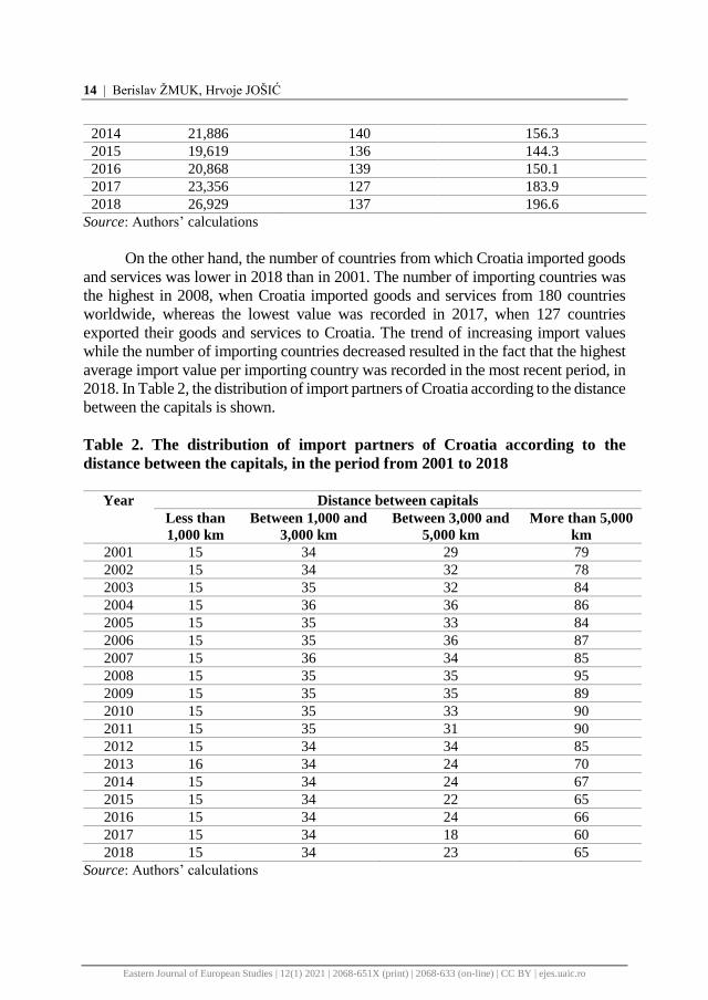
On the other hand, the number of countries from which Croatia imported goods

and services was lower in 2018 than in 2001. The number of importing countries was

the highest in 2008, when Croatia imported goods and services from 180 countries

worldwide, whereas the lowest value was recorded in 2017, when 127 countries

exported their goods and services to Croatia. The trend of increasing import values

while the number of importing countries decreased resulted in the fact that the highest

average import value per importing country was recorded in the most recent period, in

2018. In Table 2, the distribution of import partners of Croatia according to the distance

between the capitals is shown.

Table 2. The distribution of import partners of Croatia according to the

distance between the capitals, in the period from 2001 to 2018

Year Distance between capitals

Less than

1,000 km

Between 1,000 and

3,000 km

Between 3,000 and

5,000 km

More than 5,000

km

2001 15 34 29 79

2002 15 34 32 78

2003 15 35 32 84

2004 15 36 36 86

2005 15 35 33 84

2006 15 35 36 87

2007 15 36 34 85

2008 15 35 35 95

2009 15 35 35 89

2010 15 35 33 90

2011 15 35 31 90

2012 15 34 34 85

2013 16 34 24 70

2014 15 34 24 67

2015 15 34 22 65

2016 15 34 24 66

2017 15 34 18 60

2018 15 34 23 65




Distances between countries are divided into three categories: less than 1,000

km, between 1,000 and 3,000 km, between 3,000 and 5,000 km and more than 5,000

km. This division was made in order to capture the distance effect which is present in

smaller distances and analyse whether the precision of the Distance variable will

change across its distribution. The assumption is that the Distance variable should

perform better in case of smaller distances.

Data in Table 2 leads to the conclusion that the number of countries from

which Croatia imports goods and services is almost constant in case of smaller

distances (less than 1,000 km and between 1,000 and 3,000 km categories).

However, in the case of larger distances, in categories between 3,000 and 5,000 km

and more than 5,000 km, the number of importing countries differs greatly in the

observed period.

3.2. The sign test results

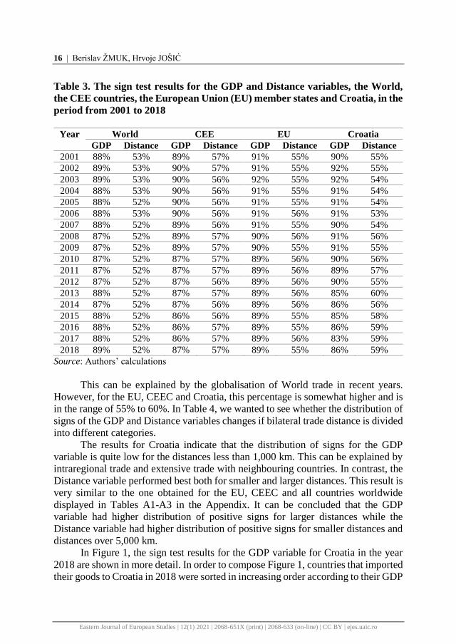
The results of conducted sign tests for the GDP and Distance variables are

displayed in Table 3. For comparison purposes, in addition to the sign test results

related to the World, in Table 3 the sign test results related to the Central and Eastern

European countries (CEEC), European Union (EU) and one individual country,

Croatia, are provided. It has to be emphasized that the category the World does not

include all countries in the World. The World category includes 174 countries

throughout the observed period. Due to the lack of available data, the World category

includes 153 countries per year on average, which is a great amount of bilateral trade

data in the observed period. For example, the dataset for the calculation of the sign

test for the World countries comprises of 363,405 entries on bilateral trade data for

the selected countries in the World. According to OECD, OECD (2019), the member

countries of Central and Eastern European countries (CEE) are Albania, Bulgaria,

Croatia, the Czech Republic, Estonia, Hungary, Latvia, Lithuania, Poland, Romania,

the Slovak Republic and Slovenia. Because of missing data for Romania, here the

CEE group of countries is not composed of 12 but of 11 countries. Similarly, because

there are no available data for Greece and Romania, the group of EU member states

here is composed of 26 instead of 28 countries.

The results of the sign test shown in Table 3 elicit the conclusion that there is

almost 90% of positive signs achieved for the GDP variable in the case of Croatia,

the EU countries, CEEC and all countries in the World which is a highly expected

result. It means that the GDP variable possesses a high predictive capability or

performance in the sign test. A country will import more from countries with GDP

higher than average World GDP and vice versa. On the other hand, the Distance

variable did not perform so well in the sign test. It correctly predicted bilateral trade

patterns in only 52% of cases for the World, which is only a little more than a coin

toss or random value.



Table 3. The sign test results for the GDP and Distance variables, the World,

the CEE countries, the European Union (EU) member states and Croatia, in the

period from 2001 to 2018

Year World CEE EU Croatia

GDP Distance GDP Distance GDP Distance GDP Distance

2001 88% 53% 89% 57% 91% 55% 90% 55%

2002 89% 53% 90% 57% 91% 55% 92% 55%

2003 89% 53% 90% 56% 92% 55% 92% 54%

2004 88% 53% 90% 56% 91% 55% 91% 54%

2005 88% 52% 90% 56% 91% 55% 91% 54%

2006 88% 53% 90% 56% 91% 56% 91% 53%

2007 88% 52% 89% 56% 91% 55% 90% 54%

2008 87% 52% 89% 57% 90% 56% 91% 56%

2009 87% 52% 89% 57% 90% 55% 91% 55%

2010 87% 52% 87% 57% 89% 56% 90% 56%

2011 87% 52% 87% 57% 89% 56% 89% 57%

2012 87% 52% 87% 56% 89% 56% 90% 55%

2013 88% 52% 87% 57% 89% 56% 85% 60%

2014 87% 52% 87% 56% 89% 56% 86% 56%

2015 88% 52% 86% 56% 89% 55% 85% 58%

2016 88% 52% 86% 57% 89% 55% 86% 59%

2017 88% 52% 86% 57% 89% 56% 83% 59%

2018 89% 52% 87% 57% 89% 55% 86% 59%


This can be explained by the globalisation of World trade in recent years.

However, for the EU, CEEC and Croatia, this percentage is somewhat higher and is

in the range of 55% to 60%. In Table 4, we wanted to see whether the distribution of

signs of the GDP and Distance variables changes if bilateral trade distance is divided

into different categories.

The results for Croatia indicate that the distribution of signs for the GDP

variable is quite low for the distances less than 1,000 km. This can be explained by

intraregional trade and extensive trade with neighbouring countries. In contrast, the

Distance variable performed best both for smaller and larger distances. This result is

very similar to the one obtained for the EU, CEEC and all countries worldwide

displayed in Tables A1-A3 in the Appendix. It can be concluded that the GDP

variable had higher distribution of positive signs for larger distances while the

Distance variable had higher distribution of positive signs for smaller distances and

distances over 5,000 km.

In Figure 1, the sign test results for the GDP variable for Croatia in the year

2018 are shown in more detail. In order to compose Figure 1, countries that imported

their goods to Croatia in 2018 were sorted in increasing order according to their GDP



values. Therefore, at the beginning of the list are countries with lower GDP values

and at the end of the list are countries with higher GDP values. In the next step, for

each country individually it was checked whether the resulting sign is equal or not

to the expected one. After that the cumulative function of correct signs was

calculated and shown in Figure 1 by the black line. The orange line represents the

perfect line. The cumulative function of correct signs and the orange line ought to be

one on top of one another if all signs are correct. The less correct the results of the

sign test are, as we move towards the right of the Figure 1, the difference between

those two lines is greater.

Table 4. The sign test results for the GDP and Distance variables for Croatia

according to distance between capitals, in the period from 2001 to 2018

Year

GDP Distance

Less

than

1,000

km

Between

1,000 and

3,000 km

Between

3,000 and

5,000 km

More

than

5,000

km

Less

than

1,000

km

Between

1,000 and

3,000 km

Between

3,000 and

5,000 km

More

than

5,000

km

2001 53% 91% 100% 94% 67% 29% 0% 84%

2002 53% 94% 100% 95% 73% 29% 0% 86%

2003 60% 91% 100% 94% 67% 29% 0% 83%

2004 60% 92% 97% 94% 73% 31% 0% 84%

2005 53% 94% 97% 94% 80% 26% 0% 83%

2006 53% 94% 97% 94% 80% 26% 0% 82%

2007 53% 92% 94% 94% 80% 28% 0% 82%

2008 53% 97% 94% 94% 80% 29% 0% 83%

2009 60% 91% 94% 94% 73% 29% 0% 84%

2010 60% 91% 94% 92% 73% 29% 0% 84%

2011 53% 91% 90% 93% 80% 29% 0% 84%

2012 60% 91% 91% 94% 67% 29% 0% 85%

2013 63% 88% 88% 87% 63% 32% 4% 93%

2014 60% 91% 92% 88% 67% 24% 0% 90%

2015 53% 91% 95% 86% 67% 26% 0% 92%

2016 47% 91% 96% 88% 73% 26% 0% 94%

2017 53% 88% 94% 85% 67% 29% 0% 92%

2018 47% 91% 96% 89% 73% 26% 0% 94%


The results from the Figure 1 indicate that the GDP variable had higher

distribution of positive signs in case of Croatian bilateral imports with countries

having the lowest gross domestic product (for the first 50 smallest trade partner

countries there was only one incorrect sign in the sign test). The elements for

construction of Figure 2 are calculated in the same way as for Figure 1, but now

using data for the Distance variable instead of the GDP variable. The Distance

variable had higher distribution of positive signs for small and larger distances, the

result already seen in Table 4.



Figure 1. The sign test results for the GDP variable for Croatia according to the

GDP value of exporter countries, in 2018

Source: Authors’ representation

Figure 2. The sign test results for the Distance variable for Croatia according

to the Distance value of exporter countries, in 2018

Source: Authors’ representation

0.0

0.2

0.4

0.6

0.8

1.0

0.0 0.2 0.4 0.6 0.8 1.0

Sh

are

of

corr

ect

sign

s

Share of countries

0.0

0.2

0.4

0.6

0.8

1.0

0.0 0.2 0.4 0.6 0.8 1.0

Sh

are

of

corr

ect

sign

s

Share of countries



In Figures A1 and A2, in the Appendix, the sign test results are observed in

more detail than in Figures 1 and 2. The importing countries were firstly split into

four groups according to their distance between capitals. The analysis was then

conducted similarly as in Figures 1 and 2, for each distance group separately. Again,

the results are very similar to the ones in Table 4; the GDP variable had higher

distribution of positive signs for distances higher than 1,000 km. Furthermore, the

Distance variable had higher distribution of positive signs for distances less than

1,000 km and distances more than 5,000 km.

3.3. The rank test results

In Tables 5 and 6 the average root mean square errors and average mean

absolute percentage errors for the GDP and Distance variables in the case of the

World, the CEE countries, the European Union (EU) member states and Croatia are

shown. It has to be emphasized that the average error values have been calculated by

summing up individual error values of importing countries from the same country

group and by dividing that sum with the number of importing countries.

Table 5. The rank test errors for the GDP variable, the World, the CEEC, the

European Union (EU) member states and Croatia, average by country, in the



RMSE MAPE RMSE MAPE RMSE MAPE RMSE MAPE

2001 27 70% 30 63% 29 48% 33 67%

2002 27 70% 29 61% 28 47% 30 63%

2003 27 70% 29 60% 28 46% 31 59%

2004 28 71% 31 62% 29 48% 30 56%

2005 28 73% 32 62% 30 49% 31 60%

2006 28 70% 32 61% 29 48% 33 60%

2007 28 69% 31 60% 29 48% 31 57%

2008 29 69% 31 61% 29 49% 32 56%

2009 29 68% 30 64% 29 51% 30 57%

2010 29 68% 31 69% 30 54% 30 63%

2011 29 69% 32 69% 30 55% 32 64%

2012 29 69% 32 72% 30 57% 32 67%

2013 30 69% 32 73% 30 58% 30 87%

2014 30 69% 32 78% 30 59% 30 86%

2015 29 67% 31 81% 30 61% 30 91%

2016 29 66% 31 78% 30 59% 31 88%

2017 29 66% 31 79% 30 61% 30 96%

2018 28 63% 29 74% 28 58% 29 88%




Obviously, there was no need to calculate average errors in the described way

in the case when only Croatia was observed. The results from Tables 5 and 6 indicate

that both the RMSE and MAPE are higher for the Distance variable than for the GDP

variable. It means that the GDP variable can better predict bilateral trade patterns in

the gravity model than the Distance variable.

The exception is the case of Croatia where the MAPE for the Distance variable

was lower than the MAPE for the GDP variable after the year 2013, meaning that

the Distance variable was more precise in that interval in explaining bilateral trade

imports than the GDP variable. However, overall forecasting or predicting accuracy

for both GDP and Distance variables can be interpreted as poor.

Table 6. Rank test errors for the Distance variable, World, the CEEC, the

European Union (EU) member states and Croatia, average by country, in



RMSE MAPE RMSE MAPE RMSE MAPE RMSE MAPE

2001 47 149% 47 98% 55 115% 51 93%

2002 48 148% 48 99% 55 111% 51 96%

2003 48 146% 48 99% 55 111% 53 93%

2004 49 146% 50 96% 56 109% 57 98%

2005 50 147% 51 99% 56 110% 55 98%

2006 51 150% 50 99% 56 110% 57 97%

2007 51 154% 51 102% 56 111% 56 102%

2008 51 155% 50 101% 56 110% 56 97%

2009 51 156% 50 103% 56 112% 57 102%

2010 51 157% 48 101% 55 113% 53 99%

2011 52 155% 49 100% 55 111% 53 99%

2012 51 156% 49 99% 55 110% 54 100%

2013 52 159% 48 98% 55 110% 43 80%

2014 52 159% 44 92% 53 108% 41 77%

2015 52 161% 44 94% 54 111% 40 79%

2016 52 163% 44 93% 53 111% 40 79%

2017 53 164% 44 92% 53 110% 37 78%

2018 52 157% 43 94% 51 109% 39 75%


3.4. Regression analysis

Due to a different number of countries included in the observed country group,

a different number of regression models was estimated. In the case of the World,

overall 2,760 standardized multiple linear regression models were estimated (with

approximately 153 regression models per year). Eleven Central and Eastern



European (CEE) countries were included with 198 standardized multiple linear

regression models estimated. Overall, 26 European Union (EU) member states were

included in the analysis with 468 standardized multiple linear regression models

estimated, while for Croatia there were 18 standardised multiple linear regression

models. In Table 7, the statistical significance of standardized GDP and Distance

variables as well as 2,760 multiple linear regression models at 1% and 5% of

significance for the all countries in the World are presented.

Table 7. The statistical significance of standardised variables and regression

models, World

Variable/regression

model, significance

Total Yes No % of

significant

cases

zGDP, significant at 5% 2,760 2,412 348 87.39%

zGDP, significant at 1% 2,760 2,273 487 82.36

zDistance, significant at

5%

2,760 2,004 756 72.61%

zDistance, significant at

1%

2760 1,484 1276 53.77%

Regression model,

significant at 5%

2,760 2,531 229 91.70%

Regression model,

significant at 1%

2,760 2,372 388 85.94%


It can be noticed that the standardized GDP variable is significant in 87.39%

of cases, the significance level being less 5% and in 82.36% of cases the significance

level being less than 1%. On the other hand, the standardized Distance variable is

significant in lower percentage of cases than the standardized GDP variable (the

significance level less than 5% in 72.61% of cases and the significance level less

than 1% in 53.77% of cases). This result further favours the GDP variable over the

Distance variable as the more significant variable in the standard gravity regression

model. A more detailed multiple linear regression analysis is shown in Table A4 for

Croatia only, although the analysis was made for all countries worldwide but due to

paper restrictions it was not possible to show it all. The detailed analysis includes

regression results for beta zGDP and beta zDistance variables with associated

standard errors, p-values and t-statistics. In addition, data for calculated regression p

and F-values, the degrees of freedom and the coefficient of determination are

presented in Table 4. In Table 8 the percentages of cases in which the GDP or

Distance variable had the higher impact on the Imports variable are shown.



Table 8. The impact of the GDP and Distance variables in the gravity regression

model, the World, the CEEC, EU member states and Croatia, in the period

from 2001 to 2018


GDP Distance GDP Distance GDP Distance GDP Distance

2001 79% 21% 64% 36% 88% 12% 100% 0%

2002 79% 21% 64% 36% 88% 12% 100% 0%

2003 77% 23% 73% 27% 88% 12% 100% 0%

2004 81% 19% 64% 36% 88% 12% 100% 0%

2005 81% 19% 64% 36% 88% 12% 100% 0%

2006 78% 22% 64% 36% 85% 15% 100% 0%

2007 81% 19% 64% 36% 88% 12% 100% 0%

2008 85% 15% 73% 27% 88% 12% 100% 0%

2009 83% 17% 73% 27% 88% 12% 100% 0%

2010 82% 18% 64% 36% 85% 15% 100% 0%

2011 83% 17% 64% 36% 81% 19% 100% 0%

2012 88% 12% 64% 36% 85% 15% 100% 0%

2013 85% 15% 55% 45% 73% 27% 0% 100%

2014 85% 15% 36% 64% 69% 31% 0% 100%

2015 85% 15% 36% 64% 65% 35% 0% 100%

2016 84% 16% 36% 64% 65% 35% 0% 100%

2017 85% 15% 36% 64% 65% 35% 0% 100%

2018 85% 15% 45% 55% 73% 27% 0% 100%


It can be noticed that the GDP variable had higher impact on the Imports

variable than the Distance variable in approximately 80% of cases for all countries

in the World (in 2018 this percentage was somewhat higher and amounted to 85%).

For other subsample of countries, the CEE, the EU, and Croatia individually the

results are similar; the GDP variable had higher impact in the majority of regression

models. This analysis has provided new insight into understanding the performance

of GDP and Distance variables in the standard gravity model. Both the GDP and

Distance variables have been considered as the main variables in the standard gravity

model of trade with numerous papers estimating their regression coefficients. But

regression analysis itself could not get into the core of understanding the

performance and impact of variables in the gravity model, which was the idea of this

paper. It seems that the economic size of a country, represented with the GDP value,

is more important factor than the distance between countries in making a decision

with which country to trade. This is the main finding of this paper offering an

important advantage over the parametric tests of the gravity model.



Conclusion

The aforementioned analysis offers the conclusion that the GDP variable had

positive distribution of signs for bilateral trade patterns (imports) for Croatia, the EU

countries, the CEEC and all countries worldwide in almost 90% of cases, which is a

very convincing and highly expected result. On the other hand, the Distance variable

had lower positive distribution of signs on the sign test, only 52% of cases for the

countries worldwide which is barely more than a coin toss. The low percentage of

correct signs achieved in the sign test for the Distance variable means that making

decisions about which country to trade with is not conditioned on bilateral distance

between countries. For the EU, the CEEC and Croatia, this percentage is somewhat

higher and is in the range of 55% to 60%. When bilateral distances were divided into

different categories, the GDP variable performed best for larger distances, while the

Distance variable was the most precise for smaller distances. Therefore, the first

hypothesis of the paper could be partially confirmed. The results of the rank test for

both the RMSE and MAPE metrics were both higher for the Distance variable than for

the GDP variable, meaning that GDP variable performs better in the gravity model

than the Distance variable. However, overall forecasting performance for both GDP

and Distance variables can be interpreted as poor. This result further favours the GDP

variable as the more significant variable in the standard gravity regression model.

Furthermore, the GDP variable had higher impact on the dependent variable in

approximately 80% of cases when multiple linear regression models with standardised

variables were estimated, indicating that second hypothesis of the paper could be

confirmed. This result further favours the GDP variable as the more important variable

in the gravity model, meaning that patterns of trade are more dependent on the

economic size of countries than their bilateral distance. The results of the sign and rank

tests for Croatia are in line with the results obtained for the CEE and the EU countries.

The GDP variable had higher distribution of positive signs than the Distance variable.

Furthermore, the GDP variable had higher distribution of positive signs for smaller

distances while the Distance variable had higher positive distribution of signs for

smaller and larger distances. In the regression analysis for Croatia the GDP variable

had also higher impact but only up to the year 2013, after which the Distance variable

had higher impact. In order to understand that result, a more detailed analysis should

be made. The reasons for this may be the Croatia’s accession to the EU in 2013, larger

intra-EU trade, yearly changes in countries’ GDP values, etc.

The limitations of the paper are the result of the missing data for some

countries in some years, so the sample of countries had to be selected. Therefore,

only 11 CEEC and 26 EU countries were included in the analysis. Also, due to paper

length restrictions, a detailed analysis for all World countries individually could not

be shown. Further investigations in this field should be made by analysing trade

flows other than imports, countries according to their income level, implementing

various distance indicators, etc. As far as the methodology used for calculating of



the sign test, an interesting possibility would be to use the mode or median value as

anchor value instead of using the mean value.

References

Almog, A., Bird, R. and Garlaschelli, D. (2019), Enhanced Gravity Model of Trade:

Reconciling Macroeconomic and Network Models, Frontiers in Physics, 7(55), pp. 1-

17. https://doi.org/10.3389/fphy.2019.00055

Anderson, J.E. (1979), A theoretical foundation for the gravity equation, American Economic

Review, 69(1), pp. io6-i6.

Anderson, J.E. and Van Wincoop, E. (2003), Gravity with gravitas: A solution to the border

puzzle, American Economic Review, 93(1), pp. 170–192.

https://doi.org/10.1257/000282803321455214

Baldwin, R. and Taglioni, D. (2007), Trade Effects of the Euro: a Comparison of Estimators,

Journal of Economic Integration, 22(4), pp. 780-818.

https://doi.org/10.11130/jei.2007.22.4.780

Bergstrand, J.H. (1985), The Gravity Equation in International Trade: Some Microeconomic

Foundations and Empirical Evidence, Review of Economics and Statistics, 67(3), pp.

474–81. https://doi.org/10.2307/1925976

Chaney, T. (2014), The Gravity Equation in International Trade: An Explanation (retrieved

from http://www8.gsb.columbia.edu/programs-admissions/sites/programs-admissions/

files/finance/Macro%20Workshop/spring%202014/Thomas%20Chaney.pdf).

De Benedictis, L. and Taglioni, D. (2011), The Gravity Model in International Trade, in: De

Benedictis, L. and Saltici, L. (ed.), The Trade Impact of European Union Preferencial

Policies, Springer.

Deardorff, A.V. (1998), Determinants of Bilateral Trade: Does Gravity Work in a

Neoclassical World? in: Frankel, J.A. (ed.), The Regionalization of the World

Economy, Chicago: University of Chicago Press.

Disdier, A.-C. and Head, K. (2008), The Puzzling Persistence of the Distance Effect on

Bilateral Trade, Review of Economics and Statistics, 90(1), pp. 37-48.

https://doi.org/10.1162/rest.90.1.37

Eaton, J. and Kortum, S. (2002), Technology, Geography, and Trade, Econometrica, 70(5),

pp. 1741–1779. https://doi.org/10.1111/1468-0262.00352

Heckman, J. (1979), Sample Selection Bias as a Specification Error, Econometrica, (47), pp.

153-161.

Helpman, E., Melitz, M.J. and Rubinstein, Y. (2008), Estimating Trade Flows: Trading

Partners and Trading Volumes, Quarterly Journal of Economics, 123(2), pp. 441-487.

http://dx.doi.org/10.1162/qjec.2008.123.2.441

Kareem, F.O. and Kareem, O.I. (2014), Specification and Estimation of Gravity Models: A

Review of the Issues in the Literature, EUI Working Paper RSCAS 2014/74 (retrieved

from https://ideas.repec.org/p/rsc/rsceui/2014-74.html).

https://doi.org/10.3389/fphy.2019.00055

https://doi.org/10.1257/000282803321455214

https://doi.org/10.11130/jei.2007.22.4.780

https://doi.org/10.2307/1925976

https://doi.org/10.1162/rest.90.1.37

https://doi.org/10.1111/1468-0262.00352

http://dx.doi.org/10.1162/qjec.2008.123.2.441

https://ideas.repec.org/p/rsc/rsceui/2014-74.html



Kohler, W.K. (1991), How Robust Are Sign and Rank Order Tests of the Heckscher-Ohlin-

Vanek Theorem?, Research seminar in international economics, Seminar Disscusion

paper No. 212 (retrieved from https://ideas.repec.org/p/mie/wpaper/212.html).

Konstantinos, K., Karlaftis, M.G. and Tsamboulas, D. (2010), The Gravity Model

Specification for Modeling International Trade Flows and Free Trade Agreement

Effects: A 10-Year Review of Empirical Studies, The Open Economics Journal, 3(1),

pp. 1-13. http://dx.doi.org/10.2174/1874919401003010001

Kreinovich, V. and Sriboonchitta, S. (2017), Quantitative Justification for the Gravity Model

in Economics, Departmental Technical Reports (CS). 1147 (retrieved from

http://digitalcommons.utep.edu/cs_techrep/1147).

Krugman, P. (1980), Scale Economies, Product Differentiation, and the Pattern of Trade,

American Economic Review, 70(5), pp. 950-959.

Lewis, C.D. (1982), Industrial and Business Forecasting Methods, Butterworths Publishing,

London, 40.

Mayer, T. and Zignago, S. (2006), Notes on CEPII’s Distances Measures, mimeo (retrieved

from http://www.cepii.fr/CEPII/en/publications/wp/abstract.asp?NoDoc=3877).

McCallum, J. (1995), National Borders Matter: Canada-U.S. Regional Trade Patterns,

American Economic Review, 85(3), pp. 615-623.

OECD (2019), Glossary of statistical terms. CEE countries (retrieved from

https://stats.oecd.org/glossary/detail.asp?ID=303).

Ohlin, B. (1933), Interregional and International Trade, Cambridge, Mass.: Harvard

University Press, 1966.

Poissonnier, A. (2016), Solving for Structural Gravity in Panels: Yes We Can, European

Commission, Discussion Paper 040, December 2016 (retrieved from

http://ec.europa.eu/economy_finance/publications).

Salvatici, L. (2013), The Gravity Model in International Trade, AGRODEP Technical Note

TN-04, April 2013 (retrieved from http://www.agrodep.org/sites/default/

files/Technical_notes/AGRODEP-TN-04-2_1.pdf).

Starck, S.C. (2012), The Theoretical Foundation of Gravity Modeling: What are the

developments that have brought gravity modeling into mainstream economics?,

Master Thesis, Copenhagen Business School, August 2012 (retrieved from

https://studenttheses.cbs.dk/bitstream/handle/10417/3335/sarah_catherine_starck.pdf

?sequence=1).

Tinbergen, J. (1962), Shaping the World Economy: Suggestions for an International

Economic Policy, New York: The Twentieth Century Funds.

Tobin, J. (1958), Estimation of Relationships for Limited Dependent Variables,

Econometrica, 26(1), pp. 24–36.

Vanek, J. (1968), The Factor Proportions Theory: The N-Factor Case, Kyklos, (21), pp. 749-

755.

https://ideas.repec.org/p/mie/wpaper/212.html

http://dx.doi.org/10.2174/1874919401003010001

http://digitalcommons.utep.edu/cs_techrep/1147

http://www.cepii.fr/CEPII/en/publications/wp/abstract.asp?NoDoc=3877

https://stats.oecd.org/glossary/detail.asp?ID=303

https://studenttheses.cbs.dk/bitstream/handle/10417/3335/sarah_catherine_starck.pdf?sequence=1

https://studenttheses.cbs.dk/bitstream/handle/10417/3335/sarah_catherine_starck.pdf?sequence=1



Appendix

Table A1. The sign test results for GDP and Distance variables for the European

Union (EU) member states according to the distance between capitals, in the


Year GDP Distance

Less

than

1,000

km

Betwee

n 1,000

and

3,000

km

Betwee

n 3,000

and

5,000

km

More

than

5,000

km

Less

than

1,000

km

Between

1,000 and

3,000 km

Between

3,000 and

5,000 km

More

than

5,000

km

2001 68% 90% 98% 92% 61% 28% 3% 79%

2002 69% 90% 98% 93% 61% 29% 3% 79%

2003 69% 91% 98% 93% 63% 29% 3% 79%

2004 71% 89% 98% 93% 63% 29% 2% 79%

2005 72% 90% 96% 93% 64% 29% 3% 79%

2006 71% 90% 96% 93% 65% 30% 4% 79%

2007 71% 89% 94% 93% 64% 29% 3% 79%

2008 71% 87% 92% 93% 66% 30% 4% 79%

2009 70% 89% 94% 92% 66% 29% 3% 79%

2010 68% 89% 92% 91% 65% 29% 4% 79%

2011 68% 90% 92% 92% 65% 28% 4% 80%

2012 68% 89% 91% 92% 64% 29% 5% 80%

2013 68% 89% 92% 92% 63% 29% 4% 80%

2014 67% 90% 92% 91% 63% 28% 4% 80%

2015 62% 89% 94% 91% 64% 28% 3% 80%

2016 61% 89% 94% 91% 65% 28% 3% 80%

2017 62% 89% 95% 91% 65% 29% 4% 79%

2018 61% 89% 96% 91% 66% 29% 3% 79%


Table A2. The sign test results for GDP and Distance variables for the CEE

countries according to the distance between capitals, in the period from 2001 to

2018

Year GDP Distance

Less

than

1,000

km

Between

1,000

and

3,000

km

Between

3,000 and

5,000 km

More

than

5,000

km

Less

than

1,000

km

Between

1,000 and

3,000 km

Betwee

n 3,000

and

5,000

km

More

than 5,000

km

2001 59% 91% 100% 91% 63% 26% 1% 85%

2002 60% 92% 100% 92% 64% 27% 1% 85%

2003 60% 94% 100% 92% 65% 26% 1% 84%

2004 62% 91% 97% 92% 66% 26% 1% 84%



2005 64% 92% 97% 92% 65% 26% 0% 83%

2006 64% 92% 97% 92% 66% 27% 0% 83%

2007 63% 90% 95% 92% 67% 27% 1% 83%

2008 64% 91% 93% 91% 67% 27% 1% 83%

2009 61% 91% 95% 91% 68% 27% 1% 83%

2010 59% 91% 92% 90% 68% 27% 1% 84%

2011 58% 90% 91% 90% 69% 27% 0% 84%

2012 60% 88% 91% 91% 63% 26% 1% 84%

2013 60% 89% 92% 90% 65% 27% 0% 85%

2014 58% 92% 91% 90% 65% 26% 1% 85%

2015 54% 91% 94% 89% 64% 26% 0% 86%

2016 52% 91% 95% 89% 65% 27% 0% 85%

2017 53% 90% 95% 89% 66% 27% 1% 85%

2018 52% 91% 95% 90% 67% 27% 1% 85%


Table A3. The sign test results for GDP and Distance variables for the World

according to the distance between capitals, in the period from 2001 to 2018

Year GDP Distance

Less

than

1,000

km

Between

1,000 and

3,000 km

Between

3,000 and

5,000 km

More

than

5,000

km

Less

than

1,000

km

Between

1,000 and

3,000 km

Between 3,000

and 5,000 km

More than

5,000 km

2001 64% 86% 93% 90% 51% 25% 15% 69%

2002 65% 86% 92% 90% 50% 26% 15% 69%

2003 66% 87% 92% 90% 50% 25% 15% 69%

2004 67% 86% 93% 89% 50% 25% 14% 69%

2005 68% 86% 92% 89% 50% 26% 14% 69%

2006 68% 86% 92% 89% 51% 26% 15% 68%

2007 67% 86% 91% 89% 51% 25% 14% 68%

2008 68% 86% 90% 88% 51% 25% 15% 68%

2009 66% 86% 91% 88% 53% 26% 15% 68%

2010 65% 86% 91% 88% 52% 26% 14% 68%

2011 65% 86% 91% 88% 52% 25% 15% 68%

2012 64% 86% 91% 88% 53% 25% 15% 67%

2013 64% 86% 91% 89% 53% 25% 14% 67%

2014 64% 87% 90% 88% 53% 25% 14% 67%

2015 63% 87% 92% 89% 52% 25% 14% 67%

2016 62% 87% 92% 89% 52% 25% 14% 66%

2017 63% 87% 92% 89% 53% 25% 14% 67%

2018 62% 86% 93% 90% 56% 27% 13% 67%




Figure A1. The sign test results for the GDP variable for Croatia according to

the GDP value of import trade partner of a country, according to the distance

between capitals, in 2018

Less than 1,000 km Between 1,000 and 3,000 km

Between 3,000 and 5,000 km More than 5,000 km




Figure A2. The sign test results for the Distance variable for Croatia according

to the Distance value of import trade partner of a country, according to the

distance between capitals, in 2018

Less than 1,000 km Between 1,000 and 3,000 km

Between 3,000 and 5,000 km More than 5,000 km


eastern journal of european studies volume 10 issue 1 2019

Documents