THE EFFECT OF QUANTITATIVE EASING ON THE VARIANCE AND

COVARIANCE OF THE UK AND US EQUITY MARKETS

ABSTRACT

We examine the impact on the variance-covariance structure of UK and US equity markets of

the Quantitative Easing (QE) operations implemented by the Bank of England (BoE) and the

Federal Reserve (Fed). While the theory of portfolio balance suggests that QE operations

could affect markets other than those in which the operations occur, prior analysis of these

other markets is scarce. We find that while QE operations in general reduced equity volatility,

day to day operations generated spikes in volatility in UK equities. We also find that BoE

operations increased the covariance between the UK and US equity markets.

1. Introduction

The financial crisis was characterized by increased instability across financial markets and

the contagion of its effects across markets and countries. The contagion of asset return

volatility across countries during times of stressed market conditions was first highlighted by

the experience of the world-wide downturn in equity prices in October 1987. For example,

King and Wadhwani (1990) found that the correlation between equity market movements in

different countries and general levels of volatility were positively related. Understanding the

evolution of the correlations between financial assets is central to establishing the limits of

diversification, to security pricing, and to successful asset allocation. Moreover, the

instability associated with contagion across countries may deter investors, may reduce

liquidity, may increase firms’ costs of raising finance, and ultimately stall economic growth.

This study aims to determine whether the actions of QE, by both the Bank of England and the

Federal Reserve improved stability in the US and UK equity markets, whether these benefits

crossed national boundaries, and how the correlation between these markets evolved during

and after the financial crisis.

The existing literature on the effects of QE, explored in more detail in the next

section, has either concentrated directly on the immediate impact on the bond market

especially on bond yields or more generally on the impact on the macroeconomic aggregates

of output (GDP) and CPI inflation. However, changes in the supply of one asset class – as

happens under QE asset purchase programmes - can influence the price of other assets, if the

assets are imperfect substitutes.1 This portfolio balance mechanism is one of the transmission

mechanisms through which QE can influence both asset prices more generally and potentially

beyond the boundaries of domestic financial markets. This opens up the possibility for

transnational effects of QE. Bernanke (2015) argues that QE can affect other countries if

1. See Tobin (1958, 1961, 1963) for the development of the portfolio balance model.

1

increased domestic demand brings forward a rise in overseas output to meet it, and also by

lowering the global risk free rate and global risk premia. By anchoring interest rate

expectations near the zero lower bound, QE was actively promoted as a means to reduce

economic uncertainty. Theoretical work by Veronesi (1999) and Ross (1989) shows how

uncertainty resolution can impact upon asset return volatility. Taken together these theoretical

frameworks motivate our study of the potential for there to exist trans-national effects of QE

on equity market volatility.

In this study, we use a multivariate GARCH modelling framework to examine the

variance and covariance structure of the UK and US equity markets, before, during and after

the recent financial crisis. In particular, a multivariate framework is employed that permits a

dynamic covariance structure between the two markets. Included in this dynamic structure

are indicator variables for the different phases of the financial crisis and QE, and variables

representing the intensity each QE action. In addition, we consider spill-over effects into the

volatility of the French, German and Japanese stock markets. Looking first at each market in

isolation, we find significant reductions of the equity market returns in the US on specific

days of US QE1 operations that is greater than the general rise in returns that is experienced

during the entire QE1 phase. We also find a positive return response to the resumption of QE

in Japan that by contrast to US and UK QE activity was much less anticipated. Otherwise, the

impacts of the phases of QE and specific days of QE actions appear to have been anticipated

in the returns. We also find that the variance of the US equity markets were also unaffected

by the US QE operations, but for the UK, we find that days of QE operations during both the

QE1 and QE2 phases generated a significant increase in the variance of the UK equity

market. This means that although volatility in these markets fell back in general after the

commencement of QE, on specific days of actual QE activity in the UK, the volatility of

equities increased in proportion to the amount of assets being purchased under the QE

2

programmes. We also find spikes on the specific days of QE activity, during UK and US

QE1, in the equity volatility in France and Germany, neither of which was experiencing QE

at that time. In addition, the French and Japanese markets saw positive spikes in volatility

during US QE3, with the latter being so after controlling for the contemporaneous resumption

of QE activity in Japan. The German market appeared to experience a general increase in

volatility during the US QE maturity extension programme, but this was reduced to below

pre-crisis levels on days following US QE operations. For the variance-covariance structure

of the US and UK equity market, our results reveal that the BoE but not the Fed QE daily

operations increased both the volatility of equity returns in both markets and also the

covariance between the two markets.

The remaining sections of the paper are as follows. Section 2 provides a brief

overview of related literatures on the covariation between equity markets, the effects of

macroeconomic policy on equity markets and the effects of quantitative easing on financial

markets. These establish context and identify the ways in which our paper contributes to the

literature. Section 3 describes the GARCH modelling framework that will be employed, and

highlights the particular innovations in our modelling that enable us to examine the effects of

QE. In Section 4, we describe the data used and provide some summary statistics. An analysis

of the estimated coefficients of the GARCH models is reported in Section 5. Section 6

contains a summary and offers some conclusions and policy implications.

2. Literature Review

2.1 Equity Market Covariation

Studies of the covariation between asset markets were greatly advanced by the

development of multivariate generalised autoregressive conditional heteroscedasticity (MV-

GARCH) time series models, as applied, for example, by Hamao et al. (1990), Koutmos and

3

Booth (1995), Bekaert and Harvey (1995) and Bekaert and Wu (2000). For example, Hamao

et al. (1990) discovered that shocks to the volatility of financial market returns in one country

could influence both the conditional volatility and the conditional mean of the returns in

another country. Berben and Jansen (2005) pioneered the use of time varying correlation

structures within the MV-GARCH model to study changes in the level of international

integration of equity markets, while Capiello et al (2006) used the dynamic conditional

correlation (DCC) model of Engle (2002) to explore the asymmetries in the dynamics of

global equity and bond markets.2 More recently, Johansson (2010) examined asset markets in

both the Asia-Pacific region and Europe, and found during the recent financial crisis, that

there were increases in correlation among stocks in both regions, but also there were

increases in markets that were relatively more insulated during these times, such as China.

Kasch and Caporin (2013) extend the model of Capiello et al (2006) to accommodate

threshold changes in correlation that depend on changes in variance. Our model has threshold

changes that depend on the transition through certain time periods corresponding to the crisis

and the phases of quantitative easing.

2.2 Macroeconomic news and equity market volatility

In an efficient financial market, macroeconomic news should be fully and instantaneously

reflected in market prices (and returns). Ross (1989) used a no-arbitrage martingale

theoretical asset pricing framework to establish that asset price volatility represents the rate of

information flow into an efficient market. Higher volatility implies a higher rate of flow of

information into prices and thus a more efficient market. The relationship between financial

market volatility and macroeconomic news, in particular, is developed in the theoretical work

of Veronesi (1999). In this model, if the uncertainty surrounding macroeconomic 2. Carrieri et al (2007) argue, however, that correlation is likely to be a conservative measure of international financial market integration. Diebold and Yilmaz (2009) have proposed an alternative method to the GARCH framework to capture spill-overs of volatility shocks from one country to another, using a VAR and aggregating volatility spill-overs from multiple other countries’ equity markets into a single index. A recent application to spill-lovers between currency and equity markets is Grobys (2015). In our study, we are concerned with “spill-over” effects of QE activity rather than spill-overs of volatility.

4

fundamentals is high, then news causes asset prices to move much more than when this

uncertainty is lower.

The empirical literature on the effects of macroeconomic news announcements on

stock prices has an extensive history, for example, Brealey (1970), Officer (1973), Rozeff

(1974), Goodhart and Smith (1985), Campbell (1987), Cutler et al (1989), Schwert (1989a,b)

and Wasserfallen (1989). More recent contributions to the literature relating conventional

monetary policy surprises and other macroeconomic news on returns in stock markets and

volatility in stock markets both within and across countries include, Becker (1995), Hamilton

and Lin (1996), Bomfim (2003), Ederington and Lee (1993), Steeley (2004), Graham et al.,

(2003), Kearney and Lombra (2004), Nikkinen and Sahlström (2001, 2004a, 2004b, 2006),

Brenner et al (2009) and Bekaert et al (2013).3 Our paper adds to this literature by examining

the impact of monetary policy actions during the recent crisis and QE phases on the volatility

of and cross correlations between the UK and US equity markets.

2.3 Quantitative Easing and Financial Markets

In March 2009, the BoE monetary policy committee (MPC) announced the start of its

asset purchase programme, financed by the electronic creation of money, at the same time as

it reduced Bank Rate to 0.5%, its effective lower bound. The QE program in the UK was in

three phases. The first phase, QE1 was between March 2009 and January 2010, when £200

billion was expended on purchase of assets, mostly gilts. The purchases of gilts were initially

restricted to conventional gilts with a residual maturity between 5 and 25 years but at the

August MPC meeting the maturity range of gilts to be purchased was brought forward to

three years and over. Other assets such as commercial paper and corporate bonds were also

purchased by the BoE but in significantly lesser quantities. In October 2011, the second

3. This is a very small selection from a vast literature that to review would encompass an entire paper in itself. There are also parallel literatures examining the effects of news on bond market returns and on volatility, for example, Jones et al (1998), Balduzzi et al., 2001, De Goeij and Marquering (2006), Brenner et al (2009), Nowak (2011) and Abad and Chulia (2013). Steeley and Matyushkin (2015) consider the effects of QE on bond market volatility.

5

phase of the quantitative easing (QE2) started and between October 2011 and May 2012 the

BoE purchased an additional £125 billion of gilts. In July 2012, the MPC announced a further

£50 billion of gilt purchases to run till November 2012 (QE3). Cumulatively, the £375 billion

of asset purchases accounts for around 35 per cent of total amount of gilts in issue

The decision by the Federal Reserve to make large scale asset purchase (LSAP) came

in two steps. The first, in November 2008, when the Fed announced purchases of housing

agency debt and agency mortgage-back securities (MBS) of $600 billion. The second came in

March 2009, when the Federal Open Market Committee (FOMC) decided to increase the

purchases of agency-related securities by additional $850 billion and to also purchase longer-

dated Treasury securities to the tune of $300 billion. In total, these purchases would comprise

22 per cent of the stock of longer-term agency debt, fixed-rate agency MBS, and Treasury

securities outstanding. The operations (LSAP1), which were extended to March 2010,

became known as QE1. However, as the financial crisis worsened, the Fed started a second

round of LSAP (QE2) in November 2010, which brought about additional purchases of $600

billion in longer-term Treasury bonds until the middle of 2011. The Fed on September 21

2011, announced a new maturity extension programme (MEP). Under the programme, the

Fed would buy an additional $400 billion in Treasury securities with remaining maturities of

6 to 30 years, while selling an equal amount of Treasuries with remaining maturities of 3

months to 3 years. The implementation of the Fed’s LSAPs was carried out by the Federal

Reserve Bank of New York under delegated authority from the FOMC.

Towards the end of our sample period, in April 2013, the Bank of Japan announced

the start of a programme of qualitative and quantitative easing (QQE). The operational target

of monetary policy was changed from the overnight call rate to the monetary base, with the

latter to increase at an annual pace of 60-70 trillion yen. Purchases of government bonds

would increase by 50 Trillion Yen annually. The qualitative aspect refers to an extension of

6

the maturities of government bonds purchased as well as the extension to other asset classes

including exchange traded funds and real estate investment trusts. 4

Existing research on the effects of the QE operations has mostly focussed on the

immediate impact in the bond market or on the impact on output (GDP) and CPI inflation.

Studies by Meier (2009), Joyce.et.al. (2011), Meaning and Zhu (2011) and Breedon et.al.

(2012), find significant reductions in bond yields in the UK resulting from asset purchases

during the first phase of QE. By contrast, Joyce et.al. (2012), Martin and Milas (2012) and

Goodhart and Ashworth (2012), which considered the QE2 and QE3 periods in the UK, and

Meaning and Warren (2015) suggest that these later QE operations did not reduce

government bond yields by as much or at all. For the US bond market, D’Amico and King

(2010), Gagnon et.al. (2011), Glick and Leduc (2012) and Hamilton and Wu (2012), Bauer

and Rudebusch (2014) and Neely (2015) found evidence of yield reductions of up to 100

basis points from the first phase of US QE. Like in the UK, later phases of QE have had more

modest effects, see for example, Swanson (2011, 2015). Studies and surveys of the wider

economic impacts of the QE operations in the US and UK include Baumeister and Benati

(2010), Lenza et.al. (2010), Kapetanios et.al. (2012), Chen et.al (2012), Bridges and Thomas

(2012), and Lyonnet and Werner (2012), Churm et al (2015), Bhattarai and Neely (2016),

Weale and Wieladek (2016) and Haldane et al (2016), with the latter two studies indicating

that the positive effects on GDP and CPI may be larger than reported in the earlier studies.

However, since the pioneering work by Tobin (1958, 1961, 1963), it has long been

understood that changes in the supply of one asset class can influence the price of other

assets, if the assets are imperfect substitutes. This portfolio balance mechanism is one of the

transmission mechanisms through which QE can influence both asset prices (generally) and

the wider economy, and provides theoretical grounding and motivation for our study of the

4. Timeline summaries of QE announcements and key events for the UK, the US and Japan can be found in Borio and Zabai (2016, Table 3).

7

effect of QE on equity market volatility and covariation.5 The direct upward pressure on bond

prices that may come from the central bank’s bond purchases can give rise to an additional

effect to increase the prices of other assets if the sellers of bonds do not regard the cash

received as a perfect substitute for the bonds sold, and use the cash proceeds to purchase

other assets, such as equity. This process may continue until all asset prices have been bid

upwards to rebalance asset portfolios to accommodate the increased cash balances. The

increase in asset prices, which leads to both wealth effects and lower costs of capital, in turn

boosts the economy through increased investment and consumption. A recent study by

Haldane et al (2016) suggests that the effects of QE on equity returns in the UK are mixed,

sometimes positive and sometimes negative and are small in magnitude. Evidence in

Villanueva (2015) draws a similar conclusion for the effects of QE on US stocks. By contrast,

Ballati et al (2016) suggest that the effects on equity prices are stronger and the pass-through

to the economy insignificant. Barbon and Gianinazzi (2017) report a significant increase in

Japanese equity prices in response to the purchase of ETFs by the Bank of Japan after 2013.

As a general policy tool, QE was designed to reduce uncertainty and improve

liquidity, and the models of Ross (1989) and Veronesi (1999) provide a theoretical channel

through which the trans-national effects of QE can influence asset return volatility. It is,

therefore, upon volatility rather than returns (where for example Haldane et al (2016) find a

limited response) that we focus our study.

Our study will add to a small number of studies that have examined the effects of QE

on equity market volatility, although these have all been confined to studying the effects

within a single country. Tan and Kohli (2011) examine the volatility of the US stock market

over the period 2008 to 2011, encompassing the US QE1 and QE2 phases. They examine

three models of volatility, an AR(1) process and a modified constant elasticity of variance

5. QE may also influence the economy through liquidity and expectations based transmission channels. These are described in, for example, Benford et al (2009).

8

model, both applied to the VIX measure of implied volatility for the S&P500 index, and the

conditional volatility from a GARCH(1,1) model applied to the returns to the S&P500 index.

They find that the onset of QE led to a significant drop in stock index volatility that then

reverted to previous levels following the ending of a phase of QE. Joyce et al (2011) examine

the behaviour of the option-implied volatility of the FTSE100 index between January 2009

and June 2010, a period encompassing the UK QE1 phase. They found that the twelve-month

implied volatility fell by around 40% during 2009. They also constructed an option-implied

probability distribution for the FTSE100 returns and found that it narrowed between February

2009 and February 2010, with the (lower) tail risk falling considerably. Examinations of the

tail risk of US stocks by Wang et al (2015) and Hattori et al (2016) also suggest that QE

dampened stock return volatility.

Joyce et al (2011) also consider the possibility of time variation in the correlation

structure between asset classes. They use a diagonal VECH form of the multivariate GARCH

and offer some preliminary evidence, using monthly data until the end of 2009, of increases

in the volatility of the correlation between UK equities and bonds around the commencement

of QE. However, the estimated conditional covariances appear to display some instability

with the onset of the crisis, and the lack of statistical significance of some of the coefficient

estimates, particularly in the unconditional variance-covariance matrix suggests that their

model may be poorly specified. Steeley (2015) develops this analysis further by including all

the phases of QE in the UK, isolating their separate effects, using daily data, measuring the

intensity of QE activity on a particular day and including additional macroeconomic controls.

The QE intensity measure captures the actual size of QE activity on a particular day, to

determine whether this has an effect beyond a general effect of the markets being within a

phase of QE. He is unable to reject the hypothesis that the correlations among UK asset

classes did not change during the period 2004 to 2014.

9

In this study, we will extend and refine this earlier work in a number of important

dimensions. First, we will broaden the analysis to more than a single country. This will

enable us to see if QE activity effects not only the equity market volatility of the country

within which the QE activity took place (the UK or the US) but also had an effect on

volatility in another country that was not experiencing QE, specifically France and Germany

and Japan. Japan actually resumed quantitative easing towards the end of our sample period,

and so we also examine whether this had any incremental impact. The existing research on

QE spill-over effects has focused on the effects of US QE on supporting asset prices (rather

than volatility) and the economy, for example Fratzscher et al (2013), Rogers et al (2014),

Neely (2015), Haldane et al (2016) and Chen et al (2017),6 and so our study provides an

insight into possible spill-overs into volatility.

Second, by combining the UK and US into a multivariate GARCH system, we

examine whether the volatility of equity returns in these two countries and the correlation

between them is affected by the QE operations of both countries, or whether one of them

appears to dominate. Given the closely related nature and timing of the QE operations by

both the Fed and the BoE, it is interesting to disentangle their effects on volatility within and

between the two countries. Third, we include the more recent maturity extension programme

of QE2 and the QE3 phase in the US, which have been much less studied than QE1 and QE2,

to see whether their effects were different to the prior QE2 phase. Fourth, we refine the

measure of QE intensity and calculate it for both countries. Overall, our paper offers

substantial contributions to specific several existing literatures, as well as adding to the

overall body of research that has examined the effects of QE.

3. Methodology

6. There are also emerging literatures examining the spill-overs from the very recent introduction of QE by the ECB into other European economies, which happened after the end of our sample period, for example, de Santis (2016), and for spill-overs into emerging economies, for example, Burns et al (2014).

10

The generalised autoregressive conditional heteroscedasticity (GARCH) family of statistical

processes (Engle, 1982 and Bollerslev, 1986) is used to model the variance processes of the

returns in the two markets.7 Specifically, the basic model is

Ri , t=αi ,0+αi ,1 Lehmani ,t +θi ,1 D1i , t+θi , 2D2i ,t+θi ,3 D3i ,t+θ i ,4 D4i , t

+ϕi , 1QE1i , t+ϕi , 2QE2i , t+ϕ i ,3 QE3 i ,t+ϕi , 4 MEPi ,t +d1 Ri , t−1+εi , t

(1)

where εi , t|Ωt−1 N (0 , hi ,t ), where

hi , t=ωi ,i+b i ,i εi ,t−12 +c i ,i hi ,t−1+α i ,3 Lehman i ,t+γ i ,i ,1 D1i , t+γ i ,i , 2D2i ,t+γi , i ,3 D3i ,t+γi , i, 4 D4i , t+φi , i ,1 QE1i ,t+φi ,i , 2QE2i , t+φ i ,i ,3 QE3i , t+φi , i ,4 MEPi , t(2)

where Ri , t is daily the return from market i in week t , i∈US,UK, France, Germany, Japan.

The information set, Ωt−1, includes all information known at time t−1, and ωi ,i>0, b i, i ,c i ,i>0,

b i, i+c i ,i+∑j=1

4

γ i ,i , j+∑j=1

4

φ i ,i , j<1. As first observed by Fisher (1966), index returns will be

characterized by autocorrelation where the component asset returns respond with different

speed to new information and so we include an autoregressive correction for those markets

for which it is required. The variable Lehmani , t is an indicator variable that takes the value

one during the period starting with the collapse of Lehman Brothers on September 15, 2008

and ending the day before the start of QE in each country, March 10, 2009 (UK) and March

24, 2009 (US).

The variablesD 1t, D 2t and D 3t are also indicator variables capturing the effects of

entire phases of QE activity. Thus, for the UK, the variables take the value of one during the

following periods, and are zero otherwise: D 1i ,t from 11th March 2009 to 26th January 2010,

D 2i ,t QE2 from 10th October 2011 to 2nd May 2012, and D 3i ,t QE3 from 9th July 2012 to 1st

November 2012. Similarly, the corresponding periods for which these variables take the

value of one for the US phases of QE are: D 1i ,t from 25th March 2009 to 29th October 2009,

D 2i ,t from 3rd November 2010 to 30th June 2011 and the D 3i ,t from 13th Sep. 2012 to 31st Oct.

7. See also the survey paper by Bollerslev et al. (1992). Pre-testing of the returns series strongly rejected the null hypothesis of no ARCH effects.

11

2014. The variable D 4 i ,t, which is only used in the US market equations, is an indicator

variable for the maturity extension programme conducted between 21st September 2011 and

30th Jun. 2012, prior to the US QE3 phase. For the Japanese market, we additionally add an

indicator variable that takes the value 1 from the resumption of QE by the Bank of Japan on

April 4th, 2013.

The intensity of QE activity on a particular day is measured by the variables QE1t ,

QE 2t ,QE 3t and MEPt (in the US QE equations only) and are similarly separated by the

phases of QE. 8 The value of this variable on day t is the quantity of purchases on that day

relative to the average daily quantity of purchases prior to that day. We examined a number

of alternative measures of QE intensity, including the quantity of purchases on a day relative

to the total (or average) across all QE periods and our key findings do not depend on the

precise definition of the measure. 9

The form of the variance equation in equation (2) is a standard GARCH(1,1)

specification, where the conditional variance is a function of its immediate past values and

past squared residuals only, with the addition of the same exogenous variables and indicators

as appear also in the returns equation. Using this model as the null hypothesis, likelihood

ratio tests could not reject this model in favour of more complex alternative specifications

involving asymmetries, variance-in-mean terms, or higher order ARCH terms. In the variance

equation, the coefficient b measures the tendency of the conditional variance to cluster, while

the coefficient c (in combination with b) measures the degree of persistence in the conditional

variance process.

8. As the Bank of Japan only publish QE activity data on an aggregated monthly basis, it is not possible to create a corresponding intensity variable, and so only a phase dummy variable is included to capture Japanese QE.9. We acknowledge a referee of this journal for prompting us to consider a variety of measures. The advantage of using a measure relative to an average, rather than relative to a total, is that it takes the same order of magnitude as the phase dummy variables, which makes the interpretation of the estimated coefficients much more obvious. Although the bounds of forthcoming QE purchase exercises were announced at the start of each phase, the actual out-turn of purchases was not known in advance. So, to ensure the most conservative of testing frameworks, we measure intensity relative to the average of prior daily purchases, rather than the full sample average.

12

In the first stage of the empirical analysis, each of the markets is modelled separately

using equations (1) and (2). In order to capture the evolution of the correlations between the

UK and US markets, and how this has been affected by their parallel QE activity in the post-

crisis period, it is necessary to estimate the two markets together and to explicitly model the

correlation processes. Within a multivariate setting it is possible, in principle, for each

conditional variance or covariance term to depend on all the lagged variance and covariance

terms, which quickly generates a large parameter space. We use the diagonal VECH

restricted version of the multivariate GARCH model proposed by Bollerslev et al (1988),

which reduces considerably the number of parameters to estimate.

Because the time periods of the phases of QE in the UK and the US sometimes

overlap in full or in part, it is not possible to include all the QE phase variables used in the

univariate specifications into the mean equations of the multivariate specification, due to the

strong collinearity that is generated. However, we can include a sub-set that spans all of the

separate phases. So, we include a single variable that encompasses the first QE phases for

both the US and the UK. For the second phase, the original QE phase dummies can be used

as they are unique time periods. For the third phase, like with the first, the variable covers the

period from the start of the US maturity extension programme to the end of its third phase of

QE, a period that encompasses the third phase of UK QE. A similar issue arises with the QE

intensity variables, and we solve this by combining the individual QE intensity variables, on a

per country basis, into a composite variable that captures daily QE intensity in that country

throughout the entire sample period. So, we create two new variables, QEUK ,t, and QEUS ,t as

QEi , t=QE1i ,t+QE2i ,t+QE3i , t+MEPi , t i∈UK ,US (3)

and include both of them in the multivariate specifications of the means and of the variances

and covariance.10

10. Since the UK and US trading days partially overlap rather than fully coincide, it is possible that the effects of US QE operations into the UK equity market may not be captured fully using a contemporaneous variable. So, we examine the model with the US QE intensity variable lagged by one day. Our conclusions are not changed whether using lagged or

13

In this case, the variance processes are similar but simplified versions of the processes

specified in equation (2), that is

hi , t=ωi ,i+b i ,i εi ,t−12 +c i ,i hi ,t−1+α i ,3 Lehman i ,t+ei , i ,UK QEUK ,t+ei ,i , US QEU S , t−1 (4)

while the companion covariance process is specified as

hi , m,t=ωi ,m+bi , m εi ,t−1 εm,t−1+ci , m hi ,m, t−1+αi , 3Lehmani , t+e i ,m, UK QEUK , t+e i ,m , USQEUS,t−1 (5)

As we find in the univariate model that of the dummy variables representing the Lehman

collapse and the QE phases, only the Lehman dummy variable is significant in the variance

specifications, we only include the former in the multivariate variance and covariance

specifications. This aids the estimation of the multivariate model by reducing the parameters

to be estimated and avoiding collinearity issues.

A potential pitfall with the diagonal VECH specification is that the matrices of

parameters, for example, the 2×2 matrix B that has general element b i, m, i=1,2 , and m=1,2 ,

might not be positive semi-definite. The solution that we adopt is to restrict the parameter

matrices to have full rank, which guarantees positive semi-definiteness. Parameters of all of

the models will be estimated by maximum likelihood using the Levenberg-Marquardt

algorithm, which combines the Gauss-Newton method with a gradient descent method,

Levenberg (1944) and Marquardt (1963).

4. Data and Summary Statistics

Daily closing observations, adjusted for dividends, of the FTSE100, S&P500, CAC40,

DAX30 and Nikkei225 price indices were taken from Datastream. These price indices (p) are

converted to returns (r) by the standard method of calculating the log-difference, rt= log (

pt / pt−1¿ .These observations start from 2004:01 and run to 2014:10. Although the QE

operations commenced in March 2009, the choice of the sample starting period, is to enable a

contemporaneous intensity variables. We make a similar substitution in the univariate models when examining the effects of US QE in Europe, and of both US and UK QE in Japan. We thank a participant at the 2016 INFINITI conference for suggesting this additional check.

14

comparison of the variance both before and during QE for the two equity markets being

examined.

The summary statistics for the returns series, in Table 1, show that the daily mean

returns for the equity markets for the sample period range from 0.005 (France) to 0.030

(Germany) percent per trading day or about 1.24 and 12.6 percent per year, respectively, with

the UK, Japan and the USA experiencing an annual returns of between 3.34 percent and 5.04

percent on average. While the US and UK markets both had negative skewness over the

sample period, the level of skewness is small. The Japanese market displays a greater

negative skewness, while the returns in the two European markets appear to have slight

positive skewness. All the return series are leptokurtic, reflecting the fat-tailed nature of

distributions of asset returns.

In addition to the summary statistics computed for the daily returns, we also computed

the correlation coefficient between the daily equity market returns for the US and UK,

dividing the sample to provide comparative statistics for periods before and during

quantitative easing. The significance of the correlation coefficients were verified by

regressing the UK equity market returns on the US equity market returns and using the p-

values of the F-statistic from the regression outputs, which were all highly significant. A

Chow test was also performed on the full sample estimation output with the March 11 th 2009

commencement date of the first phase of the BoE QE operations as the breakpoint, with a

null hypothesis of no break on the specified date. The null hypothesis was also strongly

rejected (p=0.0001). A similar result is also obtained using March 25 th 2009, the

commencement date of the Fed’s first purchases of Treasury bonds. The correlation between

the markets increased from 54 percent prior to the start of QE to 67 percent afterwards.

QE asset purchase data were obtained from the BoE and Fed websites respectively for

the UK and the US and were calculated such that the market value of bonds purchased on any

15

given day since the start of QE, on March 11th 2009 for the UK and 25th 2009 for the US, was

divided by the average daily market value of bond purchases through the QE activity across

all QE activity days prior to the given day, for the respective country. This is taken as the

measure of QE activity intensity on a given day. Figures 1 and 2 show frequency distributions

of the sizes of the daily asset purchase quantities (relative to the prior daily average) during

the individual phases of the QE operations, for both the UK and the US. It can be seen that

the activity during QE1 in the UK spans a much wider range of relative sizes than during the

latter two phases of QE. Moreover, only QE1 saw purchase activity that was regularly

consistently larger than it had been to that point. By contrast, during QE2, the size of QE

purchase activity was more moderate, concentrated around 85 percent of the prior average

daily value, while during QE3, the activity reduced to as little as 47 percent of the prior daily

average purchase values. For the USA, the distribution of relative sizes of QE purchase

activity covers a broader range, from as little as 3 percent of the prior average to more than

twice that average on two occasions. Moreover, there is less distinction between the phases

than for the UK, except for a slight tendency for relative larger scale activity during QE2 and

somewhat smaller scale activity during QE3, which itself saw the most actions with it being

the most long lasting phase.

5. Empirical Results

Tables 2 and 3 present the estimates of the parameters of the models in equations (1) and (2).

Table 2 contains the estimated parameters of the mean equation, equation (1), while Table 3

contains the estimated parameters for the variance equation, equation (2). Each table has an

upper and a lower panel. The upper panel relates to QE activity in the UK, while the lower

panel relates to QE activity in the US. Each panel features the country undertaking QE (the

UK or the US) and then the three other countries France, Germany and Japan.

16

Given that UK and US QE activity was heavily anticipated, our prior expectation is

that the impacts will be concentrated in the variance rather than in the mean. This is broadly

what we see in the mean equations, although there are some interesting exceptions. Although

not significant, the indicator variable capturing the impact of the Lehman Brothers collapse is

associated with a reduction in returns in all countries examined. The phases of UK QE have

no significant effect on equity returns, which is consistent with recent findings in Haldane et

al (2016), and the variables measuring the intensity of QE activity have only a spill-over

effect into the returns in the German equity market. During QE1, UK QE activity is

associated with a significant rise in the returns in German equities (p=0.09), while during

QE3, UK QE purchases appear to be reducing returns in German equities (p=0.05). During

QE1 in the US, the entire phase of QE is associated with a rise in US equity returns (p=0.06),

but this is more than offset by a reduction in returns on the days of actual QE activity

(p=0.04). The observations of negative reactions to QE activity are in conflict with the

portfolio rebalancing transmission channel of QE, in that investors that have sold bonds into

the QE process are then seeking alternatives to replenish their portfolios, which puts upward

(rather than downward) pressure on prices.11 Therefore, we considered the possibility that the

reaction on the day of QE purchases could be a correction to an overreaction the previous

day, in response to anticipatory purchases of equity. We added an indicator variable that took

the value one the day before a QE operation, but found no significant effect and also no

change to the negative and significant response on the day itself. However, this negative

reaction is consistent with findings for UK QE reported in Joyce, Liu and Tonks (2014) that

investors in gilts who were selling into the QE purchase programme were also selling off

equities, replacing both with corporate bonds. It is possible, therefore, that US investors were

replacing both government bonds and equity with corporate bonds during QE1. Later phases

1111. These results are robust to the alternative measures of QE activity that we examined and to other minor specification alterations for both the mean and variance equations and to alternative distributional assumptions and optimisation algorithms.

17

of US QE do not seem to influence US stock returns, which is consistent with findings in

Villanueva (2015). In the case of Japan, we find a positive and significant effect on returns of

the third phase of US QE, (p=0.03). However, as this phase fully encompasses the re-starting

of QE in Japan, it is most likely that this is a positive reaction to its own renewed QE activity

that, by contrast to the UK and US’s responses to the financial crisis, was much less

anticipated.12 This is consistent with the portfolio rebalancing channel of QE, and the recent

study by Barbon and Gianinazzi (2017).

Turning to the variance equations, in Table 3, the coefficients of the lag squared

return and the previous conditional variance terms are also highly significant and within the

expected range for all of the equity markets, with the bulk of the effect coming from the

previous conditional variance. Indicator variables for the Lehman Brothers collapse are

significant in all variance equations and, as expected, positive implying that this event period

was followed by an increase in volatility in these equity markets.

If the subsequent periods of the quantitative easing acted to reduce volatility back to

its pre-crisis levels, we should expect that the indicator variables for the phases of QE should

be not significantly different from zero. With the exception of the second UK phase of QE

where for the UK equity market the volatility was actually reduced significantly below pre-

crisis levels (p=0.03), volatility in all four countries retreated to pre-crisis levels during the

phases of UK QE. However, the QE intensity variables point to some disruption to the market

on days of QE activity. Specifically, for the UK equity market, both during QE1 (p=0.08) and

QE2 (p=0.03), there were significant increases in volatility in proportion to the size of the QE

purchases being undertaken. In addition, we find spill-over effects of these daily UK QE

purchases into the equity markets into both France (p=0.06) and Germany (p=0.03) during

1212. Although, we also include a variable to capture the precise sub-period of Japanese QE, which turns out to be negative, the net effect (including the US QE3 variable) is still positive.

18

QE1 that, as described earlier, saw the highest frequency of relatively large QE purchase

activity in the UK.

For the US phases of US QE, which in part overlap with those of the UK, we again

find, as expected, a return of volatility to pre-crisis levels, in both the US and the other three

countries. However, we find that the maturity extension programme in the US appears to

have been accompanied by an increase in the volatility of German equities (p=0.03), although

this is more than offset on days of actual QE purchases (p=0.08). We also see that days of US

QE activity also spilled –over into the German equity market (p=0.03), as was also the case

for days of UK QE activity. We also find that QE3 activity in the US spill-over to increasing

volatility in both the French (p=0.04) and Japanese markets (p<0.001), the latter even after

accounting for its own QE activity. By contrast to the experience of the UK, where QE

purchase days were accompanied by increased equity market volatility, the same is not

observed in the US, suggesting that the US equity market was more able to absorb QE related

trading.

Figure 3 plots the estimated conditional volatility for the UK and US equity market

returns over the sample period. Clearly the period depicted can be subdivided further into a

pre-crisis and QE period. The pre-crisis period starting from 2004 sees relatively low equity

market volatility in both the UK and US markets. Although there appeared to be a spike in

the UK equity market volatility in the last quarter of 2007 to the first quarter of 2008

following the run and subsequent state take-over of Northern Rock, no such spike was

observed for the US equity market at that time. It was not until September 2008, following

the bankruptcy of Lehman Brothers that both equity markets simultaneously witnessed a

surge in volatility, officially signalling the beginning of the financial crisis. The start of QE1

around the first quarter of 2009 coincided with a lowering of equity market volatility in both

markets. The termination of QE1 by both monetary authorities almost immediately saw a rise

19

in volatility in both equity markets. Susbequent QE operations (QE2) again appeared to have

calmed equity market volatility, although there were some noticeable spikes in the equity

markets’ volatility particularly for the US market around the last quarter of 2011. However

barring this, equity market volatility had largely returned to pre-crisis levels in both markets

by the end of our sample period. This is consistent with the significance levels of the QE

related coefficients in conditional variance equations, although this might not be wholly

attributable to the QE operations, given some of the other policy measures being

implemented by the two countries over this period.

We turn now to a joint analysis of the US and the UK equity market to see how each

market’s return volatility and the correlation between them was responding to each other’s

QE activity. Revisiting the mean equations first, in the upper panel of Table 4, we again find

that the first phase of US was associated with a boost to US equity returns (p=0.03), and that

the UK now also appears to be responding to this first phase of QE (p=0.05). For the US, this

significant rise in returns seems to continue beyond their first phase of QE into the period

when the UK was undertaking its second phase of QE, indicating some potential spill-over

effects, consistent with the portfolio rebalancing channel, from the UK to the US (p=0.02). In

the univariate models, a puzzling result was the observation of significant negative responses

of returns to daily QE1 activity in the US. Within the broader multivariate setting, the

evidence of this is much weaker, (p=0.34) although now we are using composite intensity

variables – which group the activity across all phases of QE.

The lower panel of Table 4, shows the estimation results of the variance-covariance

specification from the DVEC model. The coefficients on the own past shocks and own past

variance are significant and, for the conditional variances, consistent with the values obtained

in the univariate cases (p<0.0001). The dummy variable capturing the impact of the financial

crisis indicates that the crisis increased not only the conditional variances in the US and UK

20

equity markets, as we found in the univariate modelling, but also significantly increased the

covariance between the equity returns in the two countries (p=0.01). This is consistent with

our summary statistics that suggested that the post-crisis correlation between the two markets

was significantly increased. It is also consistent with the literature on financial market

contagion; in times of crises financial markets are more likely to move together.

For the effects of daily QE activity, we find results that augment the findings of the

univariate modelling in important ways. First, as with the univariate modelling, the daily QE

activity in the US had no impact on US equity volatility. We now can also see that it had no

effect on either the volatility of UK equities or the covariance between US and UK equities.

In the univariate case, we found that UK QE activity impacted UK equity volatility in both

the first and second phases of QE, and our composite variable picks this up again in the

multivariate setting (p=0.09). But, what we also find in the multivariate setting is that daily

QE activity in the UK is spilling over into both the volatility of US equities (p=0.09) and also

the covariance between the two markets (p=0.07), increasing them all. The conditional

correlation derived from the conditional variances and covariance from the multivariate

model is shown in Figure 4. The rise in the conditional correlation that follows the financial

crisis is clear, and consistent with the results for the unconditional correlation reported in

Section 4. We can also see that this rise begins to decay during the phases of QE that follow.

6. Conclusion

Our study has examined the effects of US and UK QE operations, both in general and

of the intensity of daily bond purchase activity by the monetary authorities, on the volatility

of their equity market returns. This has been done both within each market and, by using a

multivariate GARCH model, permitting QE effects to transfer from one market to another,

and to also influence the cross market correlation in returns. We also consider the potential

21

for QE effects to spill-over into other countries that were not experiencing QE activity as an

immediate response to the financial crisis.

Our empirical results suggest that QE operations have had some significant impact on

the equity markets examined. Consistent with recent studies that have examined the effects

of QE on equity returns, our results from the univariate analysis indicate that QE operations

mostly had relatively little impact on returns not only in the UK and US, but also in France

and Germany that were not undertaking QE or in Japan that only resumed QE activity very

recently. However, there was some indication that German equity returns were responding

positively to UK QE daily activity during QE1 and QE3, while Japanese equities seemed to

respond positively to the resumption of their own QQE programme in 2013.

Across all markets, the most dramatic result is the significant rise in the volatility of

equity returns following the collapse of Lehman Brothers, from which many have dated the

start of the financial crisis. Equally dramatic is the subsequent reversal of this rise once the

UK and the US commence their QE operations. In all countries, volatility returned to pre-

crisis levels during the phases of UK and US QE. For the UK, volatility actually decreased

significantly below these levels during QE2. This suggests that QE operations not only

calmed equity markets in the countries that were undertaking QE operations but also did so

more widely, in Europe and in Japan. The intensity of daily QE activity in the UK was also

found to cause increases (on those days) in the volatility of UK equity returns in the UK

during QE1 and QE2, and the daily activity during QE1 also spilled over into daily volatility

increases in France and Germany. This suggests that the additional financial market trading

caused by the QE operations in the UK (through a portfolio rebalancing channel) was causing

spikes in volatility in equity returns in these three countries, meaning that the success that QE

had in dampening down the increase in volatility experienced during the financial crisis was

22

intermittently disrupted by the effects of the QE operations themselves. US QE activity was

observed to have little effect on equity market volatility, including in the US itself.

Our multivariate analysis supports the conclusions of our univariate analysis but

allows us to consider the impacts of QE between the UK and US, who were both undertaking

their QE operations in response to the financial crisis. As foreshadowed by the univariate

analysis, we find effects coming from UK QE operations but not from US QE operations. In

particular, we find that UK QE operations not only affected UK equity volatility, but also

significantly increased US equity volatility and also the covariance between the two

countries’ equity returns. While these effects are for daily QE intensity, we also find that the

correlation between the two countries returns increased in the aftermath of the financial crisis

but that this correlation has fallen back somewhat over the course of QE.

We attribute the differences between the volatility responses to UK and US QE to the

subtle differences in programme design. As the UK was the first to start government bond

purchase operations, this may have had a disproportionate impact on financial markets

compared to subsequent QE activity in either the US or the UK. Second, the layout of QE

activity in the UK and the US were somewhat different. In the UK, the emphasis at the start

of each phase of QE was on the size of the total purchases to be undertaken, whereas in the

US, the announcements tended to mention monthly purchase targets rather than an overall

total. The latter emphasis implies a smoother purchase sequence which may have resulted in

less disruption to financial market volatility. The distribution of relative size of purchase

activity was also much more concentrated within any given phase for the UK than for the US,

again suggesting that US QE activity was being smoothed.

Our results have clear implications for portfolio selection and diversification in and

across these equity markets for investors, since the correlation between the two markets was

changing during the crisis and the subsequent phases of QE. This is also consistent with the

23

observation in Joyce et al (2014) in the UK that investors were switching from both

government bonds and equity into corporate bonds to access new diversification

opportunities. In addition, our results provide policy makers with a greater perspective on the

potential for day to day QE operations to temporarily affect other asset markets, both

domestic and overseas.

References

Ballati, M., Brooks, C., Clements, M., Kappouy, K., (2016). Did Quantitative Easing only inate stock prices? Macroeconomic evidence from the US and UK. Available at SSRN: http://ssrn.com/abstract=2838128.

Barbon, A., and Gianinazzi, V., (2017). Large-Scale ETF Purchases and the Cross-Section of Equity Prices: Evidence of the Portfolio-Balance Channel. Available at SSRN: https://ssrn.com/abstract=2925198.

Bauer, M D and Rudebusch, G D (2014): "The signaling channel for Federal Reserve bond purchases", International Journal of Central Banking, 10, 233-289.

Baumeister, C. and Benati, L. (2010). ‘Unconventional monetary policy and the great recession – Estimating the impact of a compression in the yield spread at the zero lower bound’, Working Paper Series No. 1258, European Central Bank.

Becker, G. Finnerty, J. and Friedman, J. (1995) Economic news and equity market linkages between the US and UK, Journal of Banking and Finance, 19, 1191-1210

Bekaert, G. and C. Harvey, 1995, Time varying world market integration, Journal of Finance 50, 403-444.

Bekaert, G. and G. Wu, 2000, Asymmetric volatility and risk in equity markets, Review of Financial Studies 13, 1-42.

Bekaert, G. Hoerova, M. and Lo Duca, M.(2013) Risk, uncertainty and monetary policy, Journal of Monetary Economics, Vol. 60, No. 7, 771-788

Benford, J., Berry, S., Nikolov, K. and Young, C.(2009) Quantitative easing. Bank of England Quarterly Bullentin 2009(2), 90-100.

Berben, R.P. and W.J. Jansen, 2005, Comovement in international equity markets: A sectoral view, Journal of International Money and Finance 24, 832-857.

Bhattaria, S., and Neely, C., (2016) A Survey of the Empirical Literature on U.S. Unconventional Monetary Policy. Federal Reserve Bank of St. Louis, Working Paper 2016-021A.

Bollerslev, T. (1986) Generalised autoregressive conditional heteroskedasticity, Journal of Econometrics, 31, 307-27.

24

Bollerslev, T. (1987) A conditionally heteroskedastic time series model for speculative prices and rates of return, Review of Economics and Statistics, 69, 542-547

Bollerslev, T., Engle, R.F. and Wooldridge, J.M., (1988). ‘A Capital-Asset Pricing Model with time-varying covariances, Journal of Political Economy 96(1), 116-131

Bollerslev, T., Chou, R.Y. and K.F. Kroner, 1992, ARCH Modeling in Finance: A Review of the Theory and Empirical Evidence, Journal of Econometrics 52, 5-59.

Bomfim, A. (2003). Pre-announcement effects, news effects, and volatility: monetary policy and the stock market. Journal of Banking and Finance, 27, 133-151

Borio, C. and Zabai, A. (2016), “Unconventional monetary policies: a re-appraisal”, BIS Working Papers No 570.

Brealey, R., 1970. The distribution and independence of successive rates of return from the British equity market, Journal of Business Finance 2, 29-40.

Breedon, F., Chadha, J. S., and Waters, A. (2012) ‘The Financial Market Impact of UK Quantitative Easing’, Oxford Review of Economic Policy, 28(4), 702–28.

Brenner, M., Pasquariello, P., and M. Subrahmanyam, 2009, On the volatility and comovement of US financial markets around macroeconomic news announcements, Journal of Financial and Quantitative Analysis 44, 1265-1289.

Bridges, J. and Thomas, R. (2012). ‘The Impact of QE on the UK Economy — Some Supportive Monetarist Arithmetic’, Bank of England Working Paper No. 442.

Brunner, K. and Meltzer, A. (1973). ‘Mr Hicks and the ‘‘monetarists’ ’Economica, vol. 40(157), 44–59.

Burns, A., Kida, M., Lim, J., Mohapatra, S., Stocker, M., (2014). Unconventional Monetary Policy Normalization in High-Income Countries : Implications for Emerging Market Capital Flows and Crisis Risks. Policy Research Working Paper;No. 6830. World Bank, Washington, DC.

Campbell, J.Y. (1987) Stock returns and the term structure. Journal of Financial Economics, 18, 373-399

Capiello, L., Engle, R., and K. Sheppard, 2006. Asymmetric dynamics in the correlations of global equity and bond markets, Journal of Financial Econometrics 4, 537-572.

Carriero, F., V. Errunza, and K. Hogan, 2007. Characterizing world market integration through time. Journal of Financial and Quantitative Analysis 42, 915-940.

Chen, H., Curdia, V., and Ferrero, A. (2012) ‘The Macroeconomic Effects of Large-Scale Asset Purchase Programmes’’, The Economic Journal vol. 122(564), F289–315.

Chen, Q., Lombardi M.J., Ross, A., and Zhu, F., (2017), Global impact of US and euro area unconventional monetary policies: a comparison. BIS Working Papers No 610.

Churm, R., Joyce, M., Kapetanios, G., and Theodoridis, K., (2015). Unconventional monetary policies and the macroeconomy: the impact of the United Kingdom’s QE2 and Funding for Lending Scheme. Bank of England Staff Working Paper No. 542.

25

Cutler, D., Poterba, J., and L. Summers, 1989, What moves stock prices? Journal of Portfolio Management 15, 4-12.

D’Amico, S. and King, T.B. (2010). ‘Flow and stock effects of large-scale treasury purchases’, Finance and Economics Discussion Series No. 2010-52.

De Santis, R., (2016) Impact of the asset purchase programme on Euro area government bond yields using market news. ECB working paper no.1939.

Diebold, F.-X., Yilmaz, K., 2009. Measuring financial asset return and volatility spillovers, with application to global equity markets. Economic Journal 119, 158–171.

Ederington, L., and Lee, J. (1993). How markets process information: News releases and volatility. Journal of Finance, 48, 1161-1191

Engle, R.F. (1982) Autoregressive conditional heteroskedasticity with estimates of the variance of UK inflation, Econometrica, 50, 987-1007.

Engle, R.F. (2002) Dynamic Conditional Correlation – A Simple Class of Multivariate GARCH models, Journal of Business and Economic Statistics 20, 339-350.

Fisher L., 1966, Some New Stock Market Indexes, Journal of Business, 39, 191-225.

Fratzscher, M., Lo Duca, M. and Straub, R. (2013). “On the spillovers of US quantitative easing”, Working Paper No. 1557, European Central Bank.

French, K., W. Schwert, and Stambaugh R. (1987) Expected stock returns and volatility, Journal of Financial Economics 19, 3-30.

Gagnon, J., Raskin, M., Remache, J. and Sack, B. (2011). ‘The financial market effects of the Federal Reserve’s large-scale asset purchases’, International Journal of Central Banking, vol. 7(10), 3–43.

Glick, R. and S. Leduc (2012). ‘Central Bank Announcements of Asset Purchases and the Impact on Global Financial and Commodity Markets,’ Federal Reserve Bank of San Francisco Working Paper Series, 2012-31, August.

Goodhart, C. and Ashworth, J (2012), ‘ QE: A Successful Start May be Running into Diminishing Returns’, Oxford Review of Economic Policy, 28(4), 640-70

Goodhart, C., and R. Smith, 1985, The impact of news on financial markets in the United Kingsom , Journal of Money Credit and Banking 17, 507-511.

Graham, M., Nikkinen, J., and Sahlstrom, P. (2003) Relative importance of scheduled macroeconomic news for stock market investors. Journal of Economics and Finance, 27, 153-165

Grobys, K., (2015) Are volatility spillovers between currency and equity market driven by economic states? Evidence from the US economy. Economics Letters 127, 72-75.

Haldane, A., Roberts-Sklar, M., Wieladek, T., and C. Young (2016) QE: The story so far. Bank of England Staff Working Paper No. 624, October 2016.

Hamilton, J. and Lin, G. (1996). Stock market volatility and the business cycle, Journal of Applied Econometrics, Vol. 11, 573-593

26

Hamilton, J. D. and Wu, J.C., (2012). The Effectiveness of Alternative Monetary Policy Tools in a Zero Lower Bound Environment, Journal of Money, Credit and Banking, 2012, 44, 3–46.

Hamao, Y., Masulis, R.W. and V.K. Ng, 1990, Correlations in Price Changes and Volatility across International Stock Markets, Review of Financial Studies 3, 281-307.

Hattori, Masazumi, Andreas Schrimpf, and Vladyslav Sushko. 2016. "The response of tail risk perceptions to unconventional monetary policy." American Economic Journal: Macroeconomics 8 (2): 111-136.

Johansson, A., 2010, Financial markets in East Asia and Europe during the global financial crisis, CERC working paper no.13. Stockholm School of Economics.

Joyce, M., Lasaosa, A., Stevens, I. and Tong, M. (2011). ‘The financial market impact of quantitative easing’, International Journal of Central Banking, vol. 7(3), 113–61

Joyce, M., Liu, Z. and Tonks, I. (2014). "Institutional investor portfolio allocation, quantitative easing and the global financial crisis," Bank of England working papers 510, Bank of England.

Joyce, M.A.S., McLaren, N., and Young, C. (2012). ‘‘Quantitative Easing in the United Kingdom: Evidence from Financial Markets on QE1 and QE2,’’ Oxford Review of Economic Policy, 28(4), 671-701

Kapetanios, G., Mumtaz, H., Stevens, I. and Theodoridis, K. (2012). ‘Assessing the economy-wide effects of quantitative easing’, Economic Journal, vol. 122(564), F316–47

Kasch, M., and M. Caporin, 2013. Volatility threshold dynamic conditional correlations: An international analysis. Journal of Financial Econometrics 11, 706-742.

Kearney, A., and Lombra, R. (2004). Stock market volatility, the news and monetary policy, Journal of Economics and Finance, 28, 252-259

King, M.A. and S. Wadhwani, 1990, Transmission of Volatility between Stock Markets, Review of Financial Studies 3, 5-33.

Koutmos, G. and G. Booth, 1995, Asymmetric volatility transmission in international stock markets, Journal of International Money and Finance 14, 747-62.

Lenza, M., Pill, H. and Reichlin, L. (2010). ‘Monetary policy in exceptional times’, Economic Policy, vol. 62, 295–339.

Levenberg, K., 1944, A Method for the Solution of Certain Non-Linear Problems in Least Square, Quarterly of Applied Mathematics 2, 164–168.

Lyonnet, V. and Werner, R., (2012). ‘Lessons from the Bank of England on Quantitative Easing and other Unconventional Monetary Policies’. International Review of Financial Analysis, 25, (2012), 94-105.

Marquardt, D., 1963, An Algorithm for Least-Squares Estimation of Nonlinear Parameters, SIAM Journal on Applied Mathematics 11, 431–441.

Martin, C., and Milas, C., (2012). ‘Quantitative easing: a sceptical survey’, Oxford Review of Economic Policy, vol. 28, No. 4, 750-764.

27

Meaning, J. and Warren, J. (2015), “The transmission of unconventional monetary policy in UK government debt markets”, National Institute Economic Review No. 234, November 2015

Meaning, J., and Zhu, F. (2011). ‘The impact of recent central bank asset purchase programmes’, Bank of International Settlements Quarterly Review, December, 73–83.

Meier, A. (2009). ‘Panacea, curse, or non-event: unconventional monetary policy in the United Kingdom’, IMF Working Paper No. 09 ⁄ 163.

Neely, C., (2015). "Unconventional monetary policy had large international effects" , Journal of Banking and Finance, 52(C), 101-111.

Nikkinen, J., Omran, M., Sahlstrom, P., and Aijo, J. (2006). Global stock market reactions to scheduled U.S. macroeconomic news announcements. Global Finance Journal, 17, 92-104.

Nikkinen, J., and Sahlstrom, P. (2001). Impact of scheduled U.S. macroeconomic news on stock market uncertainty: A multinational perspective. Multinational Finance Journal, 5, 129-139.

Nikkinen, J., and Sahlstrom, P. (2004a). Impact of the federal open market committee’s meetings and scheduled macroeconomic news on stock market uncertainty. International Review of Financial Analysis, 13, 1-12.

Nikkinen, J., and Sahlstrom, P. (2004b). Scheduled domestic and US macroeconomics news and stock valuation in Europe. Journal of Multinational Financial Management, 14, 201-215

Nikkinen, J., Omran, M., Sahlstrom, P., and Aijo, J., (2006). Global stock market reactions to scheduled U.S. macroeconomic news announcements, Global Finance Journal 17, 92–104.

Officer, R. (1973) The variability of the market factor of New York Stock Exchange, Journal of Business, 46, 434-453.

Poon, S., and Granger, C.W.J. (2003) Forecasting volatility in financial markets: a review, Journal of Economic Literature, 41, 478-539

Rogers, J., Scotti, C. and Wright, J. (2014). “Evaluating Asset-Market Effects of Unconventional Monetary Policy: A Cross-Country Comparison”. International Finance Discussion Papers No. 1101,Board of Governors of the Federal Reserve System

Ross, S., (1989). Information and Volatility: The No-Arbitrage Martingale Approach to Timing and Resolution Irrelevancy, The Journal of Finance 44, 1-17.

Rozeff, M. (1974) Money and stock prices, market efficiency, and the lag in the effect of monetary policy, Journal of Financial Economics 1, 245-302

Schwert, G. W. (1989a). Why does stock market volatility change over time? Journal of Finance, 54, 1115-51.

Schwert, G. W. (1989b) Business cycles, financial crises, and stock volatility, Carnegie-Rochester Conference Series on Public Policy, 31, 83-126

Shogbuyi, A.K, (2017) Quantitative Easing and Investing in Financial Asset Markets, PhD Thesis (Aston University, UK).

28

Steeley, J.M., (2004) Stock price distributions and news: Evidence from index options, Review of Quantitative Finance and Accounting, 23, 229-250.

Steeley, J.M., (2015) The effects of quantitative easing on the integration of UK capital markets", European Journal of Finance, in press.

Steeley, J.M. and Matyushkin, A. (2015). The effects of quantitative easing on the volatility of the gilt-edged market. International Review of Financial Analysis, 37, 113-128

Swanson, E., (2011): "Let's twist again: A high-frequency event-study analysis of operation twist and its implications for QE2", Brookings Papers on Economic Activity, 42, 151-207.

Swanson, E., (2015): "Measuring the effects of unconventional monetary policy on asset prices", NBER Working Papers, no 21816.

Tan, J. and Kohli, V. (2011). The Effect of Fed's Quantitative Easing on Stock Volatility, unpublished manuscript, University of California, Berkeley, available from SSRN.

Tobin, J. (1958) Liquidity preference as behaviour towards risk, The Review of Economic Studies, 25, 65-86

Tobin, J. (1961). ‘Money, capital and other stores of value’, American Economic Review, Papers and Proceedings, vol. 51(2), 26–37.

Tobin, J. (1963). A general equilibrium approach to monetary theory, Journal of Money Credit, and Banking, 142, 171-204.

Veronesi, P., (1999). Stock market overreaction to bad news in good times: a rational expectations equilibrium model, Review of Financial Studies 12, 975 – 1007.

Villanueva, M., (2015) Quantitative Easing and US Stock Prices. Available at SSRN: https://ssrn.com/abstract=2656329 or http://dx.doi.org/10.2139/ssrn.2656329

Wang, Y-C., Wang C-W., and C-H. Huang (2015) The impact of unconventional monetary policy on the tail risks of stock markets between U.S. and Japan, International Review of Financial Analysis 41, 41–51.

Wasserfallen, W., 1989, Macroeconomic news and the stock market: Evidence from Europe, Journal of Banking and Finance 13, 613-626.

Table 1: Summary statistics of the daily equity returns Jan 2nd 2004-Oct 9th 2014.

USA UK France Germany Japan

Mean% 0.020 0.013 0.005 0.030 0.013

Median% 0.070 0.024 0.042 0.090 0.000

Maximum% 10.957 9.384 10.595 10.798 13.235

Minimum% -9.470 -9.265 -9.472 -7.434 -12.111

Std. Deviation% 1.230 1.166 1.411 1.361 1.530

Skewness -0.313 -0.154 0.043 0.015 -0.649

Kurtosis 15.092 12.370 10.149 10.148 12.142

29

Jarque-Bera

(P-value)

15042

(<0.0001)

10477

(<0.0001)

5778

(<0.0001)

5775

(<0.0001)

9639

(<0.0001)

30

Table 2: Estimated Parameters of the Mean Equation for the univariate GARCH models

This table contains the estimated coefficients for the conditional mean equations from the model

Ri , t=αi ,0( j)+αi , 1( j)Lehman j ,t+θ i ,1( j)D 1 j ,t+θ i ,2( j)D2 j ,t+θ i , M DMt +θi ,3( j)D3 j , t +ϕ i ,1( j)QE1 j ,t+ϕi , 2( j)QE2 j ,t +ϕ i , M MEPt+ϕi , 3+αi , 2( j)BoJQEt+d1( j)R i ,t−1+ε i ,t

, where εi , t( j)|Ωt−1 N (0 , hi ,t ( j) j¿), and

hi , t( j)=ωi ,i( j)+bi ,i( j)εi , t−12 ( j)+c i ,i( j)hi ,t−1( j)+αi , 3( j)Lehman j ,t+γ i ,i ,1 ( j ) D1 j ,t+γi , i ,2(j) D2 j ,t+γi , i ,3 DM t+γi , i ,4( j)D3 j , t+φ i ,i ,1( j)QE1 j ,t+φi ,i ,2( j)QE2 j ,t+φi ,i , M MEPt+φi ,i , 3( j)QE3 j , t αi , 4( j)BoJQEt+μ i( j)Ri , t−1 ,

where Ri , t is daily the return from market i in week t , i∈US,UK,France,Germany,Japan. The information set, Ωt−1, includes all information known at time t−1, and ωi ,i>0, b i, i ,c i ,i>0,

b i, i+c i ,i+α i ,3+α i ,4+∑ γi , i ,k+∑ φi ,i , k+μi<1.The variablesD 1 j ,t , D 2 j , t D 3 j , t are QE phase’s dummy variables for the US and the UK. DM t is the dummy variable for the US MEP.

These dummy variables take the value of one during their respective periods and zero otherwise, j∈US,UK. The variables QE1 j ,t ,QE 2 j ,t and QE3 j , t represents the individual QE operations over

the entire QE period by the BoE or the Fed. The variable MEPt represent the QE operation twist in the US. The variable BoJQEt represents the period of quantitative and qualitative easing by the Bank of Japan. Below the estimated coefficients in parentheses are t-statistics.

Conditional Means (all estimated coefficients, except d1, are ×102)UK Quantitative Easing

Const. Crisis QE Phases QE Operations BoJ QE AR(1)α 0 α 1 θ1 θ2 θ3 θm ϕ1 ϕ2 ϕ3 ϕm α 2 d1

UK 0.0485 -0.2170 0.0780 0.1046 -0.0750 0.0424 -0.1959 -0.1353(3.220) (-1.240) (0.774) (0.706) (-0.815) (0.216) (-0.800) (-0.634) (-2.206)

France -0.0173 -0.2506 0.0041 -0.0185 0.1717 0.2547 0.1987 -0.3664(-0.868) (-1.127) (0.035) (-0.107) (1.252) (1.121) (0.555) (-1.261) (-2.915)

Germany 0.0177 -0.2130 -0.0575 0.2453 0.2222 0.4670 -0.2162 -0.6161(0.836) (-0.934) (-0.465) (1.306) (1.372) (1.683) (-0.643) (-1.955)

Japan 0.0226 -0.4830 0.0648 0.1006 -0.0868 -0.0820 0.0064 -0.0900 -0.0209(0.842) (-1.850) (0.508) (0.747) (-0.715) (-0.359) (0.028) (-0.319) (-0.295)

US Quantitative EasingUS 0.0372 -0.3575 0.2460 0.0385 0.0796 0.1180 -0.4407 0.0179 -0.1073 -0.1376 -0.0661

(1.874) (-1.579) (1.881) (0.399) (1.549) (1.352) (-2.061) (0.186) (-1.456) (-1.010) (-2.941)France -0.0171 -0.2910 0.0571 0.0122 -0.0296 0.1001 0.3865 -0.0008 0.0757 -0.2965 -0.0661

(-0.752) (-1.386) (0.446) (0.126) (-0.437) (0.617) (1.155) (-0.009) (0.700) (-1.20)4 (-2.972)Germany 0.0229 -0.3066 0.0168 0.0762 -0.0186 -0.1387 0.3454 -0.0672 0.0325 0.2255

(0.904) (-1.396) (0.112) (0.955) (-0.255) (-0.888) (1.281) (-0.900) (0.339) (0.995)Japan -0.0004 -0.2919 0.0271 -0.0182 0.2919 0.0086 0.0358 0.0199 -0.2337 0.1213 -0.2194

(-0.015) (-1.166) (0.181) (-0.140) (2.236) (0.093) (0.142) (0.206) (-1.623) (0.853) (-1.790)

Table 3: Estimated Parameters of the Conditional Variance Equation for the univariate GARCH models

This table contains the estimated coefficients for the conditional variance equations from the model

Ri , t=αi ,0( j)+αi , 1( j)Lehman j ,t+θ i ,1( j)D 1 j ,t+θ i ,2( j)D2 j ,t+θ i , M DMt +θi ,3( j)D3 j , t +ϕ i ,1( j)QE1 j ,t+ϕi , 2( j)QE2 j ,t +ϕ i , M MEPt+ϕi , 3+αi , 2( j)BoJQEt+d1( j)R i ,t−1+ε i ,t

, where εi , t( j)|Ωt−1 N (0 , hi ,t ( j) j¿), and

hi , t( j)=ωi ,i( j)+bi ,i( j)εi , t−12 ( j)+c i ,i( j)hi ,t−1( j)+αi , 3( j)Lehman j ,t+γ i ,i ,1 ( j ) D1 j ,t+γi , i ,2(j) D2 j ,t+γi , i ,3 DM t+γi , i ,4( j)D3 j , t+φ i ,i ,1( j)QE1 j ,t+φi ,i ,2( j)QE2 j ,t+φi ,i , M MEPt+φi ,i , 3( j)QE3 j , t αi , 4( j)BoJQEt+μ i( j)Ri , t−1 ,

where Ri , t is daily the return from market i in week t , i∈US,UK,France,Germany,Japan. The information set, Ωt−1, includes all information known at time t−1, and ωi ,i>0,

b i, i ,c i ,i>0, b i, i+c i ,i+α i ,3+α i ,4+∑ γi , i ,k+∑ φi ,i , k+μi<1.The variablesD 1 j ,t , D 2 j , t D 3 j , t are QE phase’s dummy variables for the US and the UK. DM t is the dummy

variable for the US MEP. These dummy variables take the value of one during their respective periods and zero otherwise, j∈US,UK. The variables QE1 j ,t , QE 2 j ,t and QE3 j , t represents the

individual QE operations over the entire QE period by the BoE or the Fed. The variable MEPt represent the QE operation twist in the US. The variable BoJQEt represents the period of quantitative and qualitative easing by the Bank of Japan. Below the estimated coefficients in parentheses are t-statistics.

Conditional Variance (all estimated coefficients, except b, c and μ are ×103)Const. GARCH(1,1) Crisis QE Phases QE Operations BoJ QE Ri , t−1

ω b c α 3 γ1 γ2 γm γ3 φ1 φ2 φm φ3 α 4 μUK Quantitative Easing

UK 0.0018 0.0977 0.8811 0.0259 -0.0067 -0.0081 0.0009 0.0290 0.0224 -0.0003(4.975) (9.896) (75.597) (2.617) (-1.463) (-2.229) (0.124) (1.755) (2.206) (-0.013)

France 0.0067 0.0407 0.9059 0.0329 -0.0020 0.0008 0.0206 0.0293 0.0176 -0.0420 -0.0025(10.343) (5.428) (84.308) (3.599) (-0.412) (0.037) (1.201) (1.952) (0.371) (-0.838) (-18.131)

Germany 0.0079 0.0487 0.8854 0.0373 0.0000 -0.0115 0.0118 0.0323 0.0512 -0.0236 -0.0019(9.543) (5.787) (70.529) (3.349) (-0.005) (-0.693) (1.012) (2.215) (1.225) (-0.731) (-14.456)

Japan 0.0088 0.0967 0.8524 0.0362 -0.0018 -0.0047 -0.0033 0.0247 0.0114 0.0043 0.0046 -0.0016(7.498) (9.518) (62.782) (2.137) (-0.287) (-0.663) (-0.336) (1.144) (0.581) (0.143) (2.793) (-10.074)

US Quantitative EasingUS 0.0025 0.0879 0.8795 0.0465 0.0045 -0.0003 0.0013 -0.0010 -0.0044 0.0007 -0.0029 0.0011

(6.384) (10.132) (72.430) (2.788) (0.933) (-0.173) (0.212) (-1.219) (-0.323) (0.374) (-0.225) (0.627)France 0.0067 0.0428 0.9032 0.0309 0.0048 0.0016 0.0168 -0.0019 0.0176 -0.0015 -0.0201 0.0056 -0.0026

(10.624) (5.886) (87.474) (3.542) (1.098) (0.735) (1.139) (-1.443) (1.159) (-0.663) (-0.624) (2.064) (-16.287)Germany 0.0087 0.0472 0.8807 0.0395 0.0015 -0.0016 0.0418 0.0006 0.0417 0.0009 -0.0659 -0.0012 -0.0020

31

(9.492) (5.504) (66.460) (3.509) (0.265) (-0.659) (2.223) (0.354) (2.218) (0.322) (-1.758) (-0.338) (-13.455)Japan 0.0116 0.0967 0.8524 0.0511 0.0005 0.0094 0.0015 -0.0147 0.0241 -0.0115 -0.0016 0.0444 -0.0016 -0.0022

(9.164) (9.036) (70.507) (2.831) (0.058) (1.389) (0.193) (-3.180) (1.037) (-1.700) (-0.249) (5.859) (0.857) (-11.416)

Table 4: Estimated parameters for the multivariate DVECH GARCH model of the UK and US equity markets

This table contains the estimated coefficients from the model

Ri , t=αi ,0+αi ,1 Lehmani , t+θi , 1 D 1t+θi , 2 ,UK D2UK ,t+θi ,2 ,US D2US ,t +θi ,3( j)D3t+ϕi , 1QEUK ,t+ϕ i ,2 QEUS ,t +d i ,1 Ri , t−1+εi , t, where

εi , t|Ωt−1 N (0 , hi ,t ), and hi , t=ωi ,i+b i ,i εi ,t−12 +c i ,i hi ,t−1+δ i ,i Lehmani , t+e i ,i ,UK QEUK ,t+ei , i ,US QEUS , t and

hi , m ,t=ωi ,m+bi , m εi ,t−1 εm,t−1+ci , m hi ,m , t−1+δ i ,m Lehmani ,t +e i ,m,UK QEUK ,t +e i ,m ,US QEUS ,t. The variables QEUK ,t and QEUS ,t are composites of the QE

operations variables across all QE phases for that country, while D 1t and D3t are composites of the first and third QE periods, respectively, across both countries. All other variables are as defined in tables 2 and 3.

Conditional Means (all estimated coefficients, except d1, are ×102)Const. Crisis QE Phases QE Operations Ri , t−1

α 0 α 1 θ1 θ2 , UK θ2 , US θ3 ϕUK ϕUS d1

US 0.0237 -0.2315 0.1658 0.2190 0.1058 0.0781 -0.1704 -0.0376 -0.2400(1.439) (-1.314) (2.309) (2.373) (1.835) (2.155) (-1.669) (-0.951) (-12.681)

UK 0.0353 -0.1859 0.1594 0.1268 0.0223 0.0075 -0.1790 0.0001 -0.0929(1.922) (-1.184) (1.961) (1.157) (0.346) (0.194) (-1.577) (0.003) (-5.120)

Conditional Variances and Covariance (all estimated coefficients, except b i, j and c i , j, are ×103)Const. Multivariate GARCH(1,1) Crisis UK QE Operations US QE Operations

ω1,1 ω2 ,i b1,1 b2, i c1,1 c2 ,i δ 1,1 δ 2 ,i e1,1 ,UK e2 ,i ,UK e1,1 ,US e2 ,i ,US

US 0.0023 0.0015 0.0819 0.0755 0.8885 0.8860 0.0444 0.0295 0.0031 0.0034 0.0004 0.0006

32

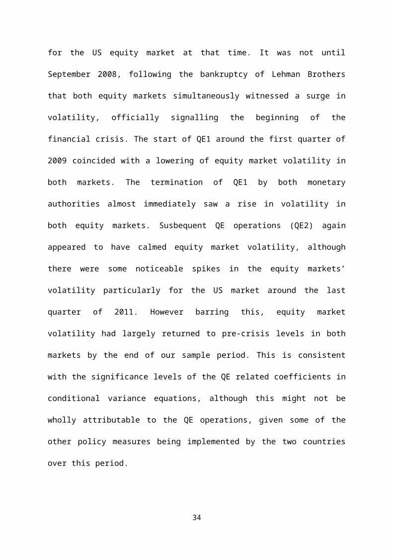
(6.814) (5.772) (10.862) (9.417) (89.403) (74.044) (2.915) (2.632) (1.656) (1.838) (0.824) (1.232)UK 0.0021 0.0864 0.8851 0.0284 0.0037 0.0009

(5.557) (10.062) (80.326) (3.034) (1.688) (1.375)

33

Figure 1: Cross-Section Distribution of QE Purchase Activity: UK

Figure 2: Cross-Section Distribution of QE Purchase Activity: US

Fig 3: Estimated Conditional Volatility for UK and US Equity Returns Jan.04-Oct.14

Fig 4: Conditional Correlation for UK and US Equity Returns Jan.04-Oct.14

35