Early Evaluation of IBM BlueGene/P

S. Alam, R. Barrett, M. Bast, M.R. Fahey, J. Kuehn, C. McCurdy, J. Rogers, P. Roth, R. Sankaran, J.S. Vetter, P. Worley, W. Yu

Oak Ridge National Laboratory

Oak Ridge, TN, USA 37831

{alamsr,rbarrett,bastm,faheymr,kuehn,cmccurdy,jrogers,rothpc,sankaranr,vetter,worleyph,wyu}@ornl.gov 

ABSTRACT. BlueGene/P (BG/P) is the second generation

BlueGene architecture from IBM, succeeding BlueGene/L (BG/L). BG/P is a system-on-a-chip (SoC) design that uses four PowerPC 450 cores operating at 850 MHz with a double precision, dual pipe floating point unit per core. These chips are connected with multiple interconnection networks including a 3-D torus, a global collective network, and a global barrier network. The design is intended to provide a highly scalable, physically dense system with relatively low power requirements per flop. In this paper, we report on our examination of BG/P, presented in the context of a set of important scientific applications, and as compared to other major large scale supercomputers in use today. Our investigation confirms that BG/P has good scalability with an expected lower performance per processor when compared to the Cray XT4’s Opteron. We also find that BG/P uses very low power per floating point operation for certain kernels, yet it has less of a power advantage when considering science-driven metrics for mission applications.

I. INTRODUCTION BlueGene/P (BG/P) [15, 16] is the second generation of

BlueGene solutions from IBM, succeeding BlueGene/L [1] (BG/L). IBM designed these systems as completely customized architectures for high performance computing that balances performance with the requirements for low power, scalability, and high density. In early 2008, BG/L systems lead the TOP500 list, holding 21 slots, with BG/P holding five slots. Ten of the top 50 systems on the list were from the BlueGene family. Perhaps more impressive is the fact that BG/P and BG/L own the top 26 spots on the Green500 list, which ranks systems by their power efficiency.

We have performed an initial evaluation of BG/P on multiple benchmarks and important scientific applications. Our experiments were performed on a two rack BG/P system located at Oak Ridge National Laboratory, and a 40 rack system located at Argonne National Laboratory. Our results compare the new BG/P architecture to DOE’s other existing large-scale supercomputer: the Cray XT [2, 3, 20].

A. BlueGene/P System Description The entire BG/P design is centered on a system-on-a-chip

(SoC) building block that has multiple networks connecting these SoCs. The SoC has four PowerPC 450 cores operating at 850 MHz. These chips are connected with multiple interconnection networks including a 3-D torus, a global collective network, and a global barrier network. The SoC has a very low power per flop ratio of 1.8 watts per GFlop/s, which contributes to the system’s ability to be packaged densely at 4096 cores per rack without the need for exotic cooling technologies (e.g., liquid cooling). In fact, other architectures have dramatically fewer cores per rack: the dual core Cray XT3 has 192 cores per rack; the quad core Cray XT4 has 384 cores per rack. A BG/P system with 72 racks (73,728 compute

nodes, or 294,912 cores) would have a peak performance of 1 PFlop/s. Although the system is a customized design, it uses standard IBM software including XL compilers, the ESSL math library, the LoadLeveler job manager, and the General Parallel File System (GPFS). Table 1 provides a configuration summary for the systems being tested.

The compute nodes contain four PowerPC 450 processor cores with 2 GB of shared RAM. Each core is a 32 bit microprocessor with a clock speed of 850 MHz. Also, each core is augmented with a double precision, dual pipe, floating point unit (a.k.a Double Hummer) that provides two fused multiply adds (FMA) per cycle, which, in turn, delivers four floating point operations per cycle for a total of 3.4 GFlop/s per core, or 13.6 GFlop/s per compute node. As a SoC, each compute node also contains hardware functionality for the memory system, the interconnection networks, and system control and debugging features. The memory system is private to each compute node; memory for other compute nodes must be accessed explicitly through the network. Within a compute node, each core has a private L1 cache of 32KB and a private L2 stream prefetching engine. All cores on a compute node share the on-chip 8 MB L3 cache, which is built from embedded DRAM. The cores also share DDR-2 memory controllers that access 2 GB of DDR-2 memory, which is off-chip. More interestingly, to improve reliability, the DDR-2 memory has been soldered onto the board, rather than using the typical DIMM slots. In contrast to BG/L, the L1 cache of BG/P is coherent, making the BG/P node a traditional cache-coherent, shared memory multiprocessor.

All five BG/P networks are connected directly to the SoC; the SoC contains all the logic and protocols to implement in each network. The five networks are a 3-D torus, a global collective tree, a global interrupt network, a 10 Gigabit Ethernet, and a JTAG control network. The 3-D torus network is the main application network on BG/P and it is used for general-purpose, point-to-point message passing and multicast operations. The torus is constructed with point-to-point, serial links between routers that are embedded within the SoC, resulting in six nearest-neighbor connections. The peak hardware bandwidth for each torus link is 425 MB/s in each direction for a total of 5.1 GB/s bidirectional bandwidth per node. This bandwidth is shared among the node’s four cores.

The global collective network has its own distinct hardware, which is separate from the torus network. Its topology is a tree; this is a one-to-all, high-bandwidth network for global collective operations, such as broadcast and reductions, and for moving data between the Compute and I/O nodes. Each Compute and I/O node has three links to the global collective network at 850 MB/s per direction for a total of 5.1 GB/s bidirectional bandwidth per node. As with the torus, the cores on a node share this network.

The 10 Gigabit Ethernet (optical) network consists of all I/O Nodes and discrete nodes that are connected to a standard 10 Gigabit Ethernet switch. The Compute Nodes are not directly

Published in SC08: International Conference High Performance Computing, Networking, Storage, and Analysis. Austin: ACM/IEEE, 2008

connected to this network. All I/O traffic is passed from the Compute Nodes, over the global collective network, to the I/O Nodes, and then, onto the 10 Gigabit Ethernet network.

Typically, applications will use the Compute Nodes in one of three modes: Symmetric Multiprocessor Mode, Dual Node Mode, or Virtual Node Mode.

Symmetric Multiprocessor mode (SMP) is the default mode of BG/P. In this mode, the Compute Node executes a single MPI task per node with a maximum of four threads within the task. Both Pthreads and OpenMP are supported, and although any thread can run on any of the four cores, each thread will be pinned to a specific core during execution.

Dual Node mode (DUAL) is a new mode in the BG/P system. In this mode, each Compute Node executes two MPI tasks per node with a maximum of four threads on the Compute Node (two per MPI task). Memory and cores are split evenly between the two tasks.

Virtual Node mode (VN) allows four MPI tasks with one thread each to run on the Compute Node. In this mode, the four cores of a Compute Node appear as different tasks (or MPI ranks). All tasks share resources on the Compute Node including memory and the networks. Optimizations in the system software allow peer tasks on a Compute Node to communicate via shared memory.

For SMP and DUAL modes, OpenMP [7] parallelism can be used to generate threads of execution for the unused cores. By default, processes are mapped to compute nodes in XYZT ordering, i.e., assigning one process to each node in the X direction of the torus, then the Y, then the Z, then returning to the first node and assigning a second process, etc. In contrast, when using VN mode the TXYZ ordering assigns processes 0-3 to the first node, 4-7 to the second node (in the X direction), etc. For DUAL mode, processes 0-1 are assigned to the first node, 2-3 to the second node, etc. In SMP mode, the XYZT and TXYZ orderings are identical. Other predefined mappings are XZYT, YXZT, YZXT, ZXYT, and ZYXT, as well as analogous orderings beginning with 'T'.

B. ORNL BlueGene/P Configuration The ORNL Blue Gene, named Eugene, is two racks (2048

compute nodes) of the standard BlueGene/P configuration. Each node has a single quad core processor, for a total of 8192 compute cores. Eugene uses the standard IBM software stack. Each rack has 16 IO nodes; each IO node serves the I/O requests from 64 compute nodes. The IO nodes are connected to each other and to disk over a 10 Gigabit Ethernet network, provided by a 256 port Myricom switch. The system uses two GPFS filesystems, one for scratch space (~ 70 TB) and a second for longer term code storage (~ 18 TB). The GPFS system includes 8 file servers and 2 metadata servers. Data is stored in 24 LUNs, each of which is approximately

3.6 TB in size. Individual LUNs are an 8+2 array of DDN disks, which communicate through dual DDN SA29500s using Infiniband.

C. ANL BlueGene/P Configuration The BG/P at Argonne National Laboratory is named Intrepid.

Its configuration is very similar to ORNL’s system, but it is much larger: 40 racks with a 64-to-1 ratio of compute nodes to I/O nodes. Also, Intrepid uses the standard IBM software, which we used for our testing; however, it can be, and often is, configured to use other system software.

D. ORNL XT Configurations Performance of the BG/P is compared to that of the Cray XT

system sited at ORNL. This Cray system, named Jaguar, has undergone rapid evolution since first installed in 2005: moving from single to dual to quad-core processors; moving from 2.4 to 2.6 to 2.1 GHz core clock speed; moving from SeaStar to SeaStar2 network interface card; moving from the Catamount compute node operating system to Compute Node Linux (CNL). The compute nodes of Jaguar have two partitions of memory modules: 667 MHz DDR2 and 800 MHz DDR2. With the current configuration of the Cray system coming online in March, 2008 and being put into production usage almost immediately, it has not been possible to collect comparable data for all of the benchmarks described in this paper. Instead, we also use data collected on earlier system configurations, as described in Table 1. For the dual-core XT4 configuration, some data were collected using the Catamount operating system, while other data were collected using CNL. The dual-core and quad-core XT systems also have execution modes analogous to those on the BG/P. In particular, for the dual-core systems, SN mode refers to assigning only one MPI process to a node, analogous to SMP mode on the BG/P. As on the BG/P, VN mode refers to assigning an MPI process to each core in a compute node. 

II. MICRO-BENCHMARKS AND KERNEL PERFORMANCE To better understand the overall performance characteristics of

a system, we employ micro-benchmarks and kernels to measure the performance of individual system components in isolation. Later, we use these measurements to understand the reasons for the observed performance of our full-scale applications.

A. HPC Challenge As part of the DARPA HPCS program [8], the design goal for

the High Performance Computing Challenge (HPCC) benchmark suite [18] was to augment the traditional LINPACK benchmark with additional tests to enable a more complete understanding of the performance characteristics of HPC platforms. HPCC tests a broad

Table 1: System Configuration Summary.

Feature BlueGene/L BlueGene/P Cray XT3 Cray XT4/DC Cray XT4/QC Node

Cores per node 2 4 2 2 4 Core Clock Speed (MHz) 700 850 2600 2600 2100 Cache Coherence Software Hardware Hardware Hardware Hardware L1 Cache / Private per core 32K 32K 64K 64K 64K L2 Cache / Private per core 14 stream

prefetching 14 stream

prefetching 1M 1M 512K

L3 Cache / Shared 4 MB Shared 8 MB Shared n/a n/a 2 MB Shared Memory per Node (GB) 0.5 - 1 2 4 4 8 Main Memory Bandwidth (GB/s) 5.6 13.6 6.4 10.6 12.8/10.6 Peak Performance (GFlop/s per node) 5.6 13.6 10.4 10.4 16.8

Interconnects Torus Injection Bandwidth (GB/s) 2.1 5.1 6.4 6.4 6.4 Tree Bandwidth (MB/s) 700 1700 n/a n/a n/a

set of node, network, and whole-system attributes that impact the performance of real-world applications. Because reference locality is often a dominating factor in application performance on modern HPC architectures, HPCC includes tests to examine how systems perform when presented with varying degrees of spatial and temporal locality. Collectively, the tests provide performance indicators for computation and communication. The HPCC suite contains 23 tests including application kernels that reflect real-world memory access patterns and interprocess communication. Several of the tests are run in three modes: single process, embarrassingly parallel, and parallel (using MPI for communication).

We ran HPCC on the Intrepid BG/P system at Argonne National Laboratory (ANL) and on its smaller cousin at ORNL, though for clarity we present BG/P results from the ANL system only. For comparison, we also ran HPCC on the quad-core Cray XT system deployed at ORNL. When setting the HPCC problem size (HPCC input parameter N) we followed guidance given by the HPCC developers and used approximately 80% of memory. Because the ORNL XT system has four times as much memory per node as the ANL BG/P system (8GB versus 2GB), each XT HPCC experiment used a problem size approximately four times larger than that used by the BG/P HPCC run with the same number of processes. We determined the blocking factor (HPCC input parameter NB) empirically; we used 144 and 168 on the BG/P and XT, respectively. For each system, we used compiler optimizations intended to leverage the architectural features of each system, such as the BG/P processors’ “double hummer” floating point unit and the Opteron’s SSE SIMD units. We used each system’s optimized math library (ESSL and ACML) but used the Fast Fourier Transform (FFT) implementation included with the stock HPCC distribution. We present only virtual node mode results here; HPCC benchmarking using SMP mode is ongoing. During the time period

we collected HPCC results, batch queue throughput was better on ANL BG/P system than the ORNL XT, allowing us to collect results for a wider range of process counts on the BG/P than the XT.

Table 2: HPCC performance comparison of BG/P with XT4/QC (VN mode, CNL) for 4096 processes.

1) Single Process and Embarrassingly Parallel Tests Table 2 shows the results of HPCC tests that are largely

independent of process count, including the single processor and embarrassingly parallel tests. The measurements in the table were taken using 4096 processes, the largest number of processes for

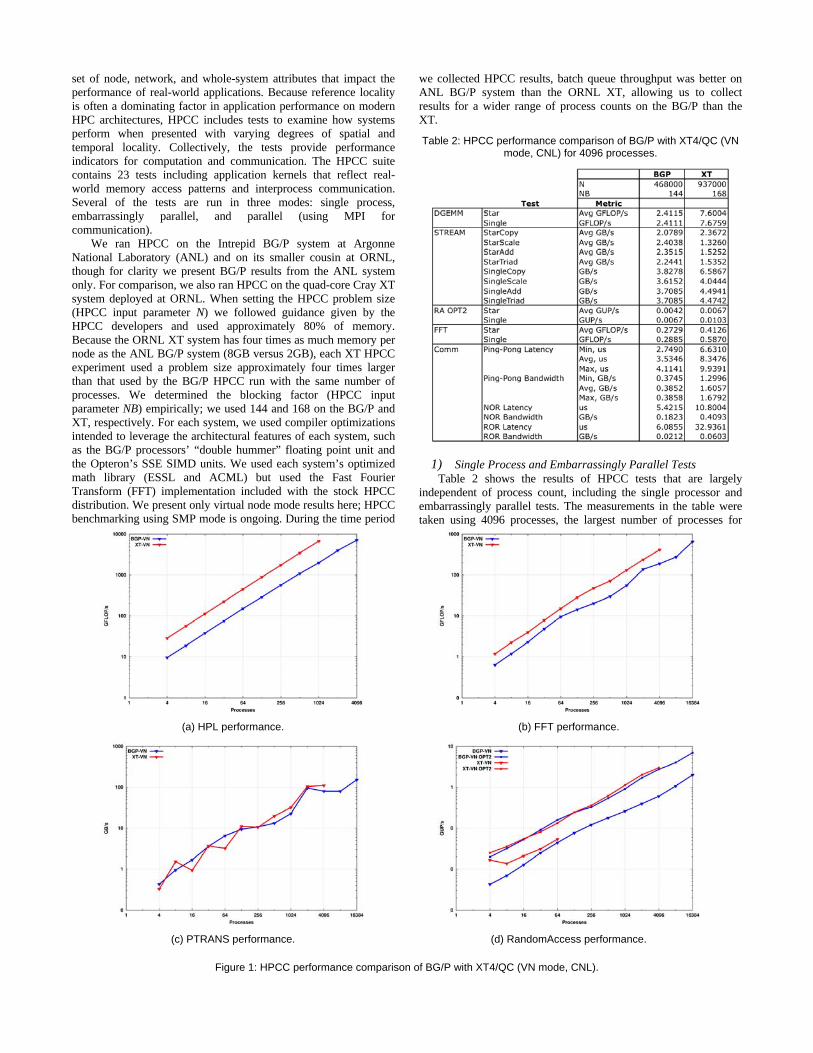
(a) HPL performance. (b) FFT performance.

(c) PTRANS performance. (d) RandomAccess performance.

Figure 1: HPCC performance comparison of BG/P with XT4/QC (VN mode, CNL).

which we obtained HPCC results on both the ANL BG/P and ORNL quad-core XT. Both the BG/P and quad-core XT can produce four floating point results per cycle, so the BG/P’s lower clock rate and smaller problem size are the likely reason for its smaller processing rate on the DGEMM and, to a lesser degree, FFT tests. The STREAM benchmark results are notable in that the BG/P exhibited higher absolute bandwidth and less of a performance decline between the single process and embarrassingly parallel cases than the XT.

2) Communication Tests In addition to single process and embarrassingly parallel

microbenchmark results, Table 2 also includes results for HPCC low-level communication tests. In general, these results match our expectations based on experience with previous BlueGene and XT generations, suggesting the BG/P network’s strength is low-latency communication whereas the XT’s strength is high-bandwidth communication.

3) Parallel Tests Figure 1 shows the result of a scaling study using the MPI

parallel HPCC tests Parallel Transpose (PTRANS), High Performance Linpack (HPL), RandomAccess (RA), and Fast Fourier Transform (FFT). HPL stresses the processor’s floating point capabilities more heavily than the other tests, and can be viewed as a demonstration of the theoretical scaling of a system. The BG/P exhibited a smaller processing rate than the XT at least in part due to its smaller clock rate and that it was solving a smaller system of linear equations, but both systems scaled well. The HPCC FFT test exhibits high temporal locality and stresses a system’s memory hierarchy and network more than HPL. Again, the XT’s larger problem size and comparable memory bandwidth account at least partially for the difference in performance between the two systems. The PTRANS benchmark exhibits high spatial locality and stresses a system’s network bisection bandwidth. Both systems exhibited similar absolute performance and scaling trends, though with a higher degree of variability on the XT. Differences in job placement strategies between the XT and BG/P resource allocator likely account for this variability; the resource allocation approach on the XT is more susceptible to fragmentation (and hence contention for the network with other applications running at the same time). Finally, the RA test is very sensitive to network latency. We measured performance using both the stock HPCC RA implementation and the “RA_SANDIA_OPT2” implementation optimized for process counts that are powers of two. The two systems showed very similar performance and scalability trends, but because RA performance tends to be better for smaller problems due to memory caching, and because of the BG/P’s smaller network latency, the observed RA performance parity was unexpected.

B. Communication To better understand the communication capabilities of BG/P,

we enlist several MPI microbenchmarks. First, we use Wallcraft HALO benchmark [26] to understand the performance impact of different strategies for mapping logical MPI tasks to BG/P cores. Second, we use the Intel MPI Benchmark suite [10], version 2.3

(IMB) to measure the performance of several popular MPI collective operations.

1) HALO Benchmark The HALO benchmark [26] simulates the nearest neighbor

exchange of a 1-2 row/column ‘halo’ from a two-dimensional (2D) array. In particular, if there are ‘N’ words on each row/column of the halo, the benchmark begins by exchanging ‘N’ words with the logically north process and ‘2N’ words with the logically south process. Once these have arrived, it then exchanges ‘N’ words with the logically west process and ‘2N’ words with the logically east process. This is a common operation when using domain decomposition to parallelize, for example, a finite difference ocean model. There are no actual 2D arrays used, but instead the copying of data from an array to a local buffer is simulated and this buffer is transferred between nodes. HALO is actually a suite of benchmarks, implementing the basic halo exchange operator utilizing a number of different messaging layers, and a number of different implementations for each layer.

We use HALO to examine three aspects of communication performance on the BG/P. The first is a comparison of different communication protocols. Figure 2(a) is a graph of performance for the indicated MPI-1 protocols on 8192 cores (VN mode) treated as a 128 by 64 virtual processor grid and using the TXYZ process mapping. Here, the x-axis indicates the number of 32-bit words in each row/column of the halo. Figure 2(b) is the same experiment on 2048 cores (SMP mode) treated as a 64 by 32 virtual processor grid and using the XYZ process mapping. Performance is graphed as a function of the amount of halo data exchanged. As can be seen, performance is relatively insensitive to the choice of protocol, though MPI_SENDRECV is slower than the other options for certain halo sizes.

The second experiment compares performance sensitivity for different process/processor mappings. Figure 2(c) and (d) compare performance between the predefined mappings TXYZ, TYXZ, TZXY, TZYX, XYZT, YXZT, ZXYT, and ZYXT for 4096 and 8192 cores, all VN mode, when using the MPI_ISEND/MPI_IRECV communication protocol. The 4096 core experiment used a 64 by 64 virtual processor grid. As can be seen, the choice of mapping is unimportant for small halo volumes. In contrast, it is important for larger volumes for these large processor grids. From these data, optimizing with respect to process/processor mapping is likely unimportant when communication is latency dominated, but may be important when communication is bandwidth limited. Results from SMP-mode experiments, not shown here, are qualitatively similar

The third experiment compares the cost of the halo exchange as a function of the virtual processor grid. Figure 2(e) and (f) compare the performance for the best mapping for each processor grid size (from among the predefined mappings) for VN and SMP modes, respectively. While there is some difference between the different processor grids, especially for halos of size between 200 and 20000 words for the VN-mode experiments, the cost does not appear to be increasing as a function of the processor grid size. This implies good scalability for the halo operator.

.

2) MPI Collective Performance Figure 3(a) and Figure 3(b) show the results of the IMB

Allreduce test that measures the latency of the MPI_Allreduce operation. In this IMB test, the Allreduce reduces a vector of float values with the MPI_SUM operator. Figure 3(a) shows Allreduce latency with 8192 processes across a range of message sizes, and Figure 3(b) shows latency with 32KB messages across a range of process counts. We measured Allreduce performance with both the stock IMB Allreduce test and a custom version that uses double precision Allreduce operands, observing a substantial performance benefit to using double precision over single precision on the BG/P but not the Cray XT. Both systems showed good scalability in terms

of message sizes and process counts, but the BG/P’s double precision Allreduce scalability was exceptional across the tested range of process counts.

Figure 3(c) and Figure 3(d) show the results of the IMB Bcast test that measures the latency of the MPI_Bcast operation. Figure 3(c) shows Bcast latency with 8192 processes across a range of message sizes, and Figure 3(d) shows the latency with 32KB messages across a range of process counts. Unlike the Allreduce test, numerical precision had no substantive impact on Bcast latency. BG/P performance scaled very well, but unlike Allreduce, the BG/P dramatically outperforms the Cray XT for all message sizes showing the benefit of the special-purpose tree network of the BG/P.

(a) (b)

(c) (d)

(e) (f)

Figure 2: BG/P HALO Performance.

C. TOP500 HPL Finally, we measured the TOP500 Linpack HPL benchmark on

BG/P. Note that the software and guidelines for the TOP500 HPL benchmark are different from those for the HPCC HPL. It was run on the ORNL BG/P using the following parameters: one problem of size 614399, block size 96, process grid size 64x128. This problem size filled approximately seventy percent of the system node memory. The result of the run was a performance score of 2.140x10e4 gigaflops, which ranked it as number 74 on the June 2008 TOP500 list. Power consumption was monitored during the run and a score of 310.93 MFLOPS/watt was calculated, which ranks this system fifth overall on the Green500 List.

III. APPLICATION PERFORMANCE In this section, we present the results for a number of important

DOE applications. The applications presented below were selected due to their importance to the mission of the Office of Science, and the completeness and understanding of results. Due to space limitations, we cannot include all results from our technical report [1].

A. Climate - Parallel Ocean Program (POP) The Parallel Ocean Program (POP) [11, 25] is a global ocean

circulation model developed and maintained at Los Alamos National Laboratory. It is used for high resolution studies and as the ocean component in the Community Climate System Model (CCSM). The code is based on a finite-difference formulation of the 3D flow equations on a shifted polar grid. POP performance is

characterized by the performance of a baroclinic phase and a barotropic phase. The 3D baroclinic phase typically scales well on all platforms due to its limited nearest-neighbor communication. In contrast, the barotropic phase is dominated by the solution of a 2D, implicit system whose performance is sensitive to network latency and typically scales poorly on all platforms. For our evaluation we used version 1.4.3 of POP with a few additional parallel algorithm tuning options (due to Yoshida [30] and to Worley). The current production version of POP is version 2.0.1. While version 1.4.3 and version 2.0.1 have similar performance characteristics, these data should not be used to imply anything about the performance of production runs of POP on the BG/P architecture. Our intent here is simply to use version 1.4.3 to identify and evaluate system performance characteristics.

We measured results for a tenth degree fixed size benchmark problem [28]. This benchmark problem uses a displaced-pole longitude-latitude horizontal grid with the pole of the grid shifted into Greenland to avoid computations near the singular points. The grid spacing is 0.1 degree in longitude (10km) around the equator, utilizing a 3600 × 2400 horizontal grid and 40 vertical levels. This resolution resolves eddies for effective heat transport and is used for ocean-only or ocean and sea ice experiments.

Figure 4 describes the POP performance when using the TXYZ ordering. The difference in performance between using the TXYZ ordering and the best observed among the other predefined mappings was less than 1.4% for VN mode and less than 1% for SMP mode. Data on fewer than 2048 nodes were collected on the ORNL BG/P system. Data on more than 2048 nodes were collected on the BG/P system in the Argonne Leadership Class Facility.

(a) IMB Allreduce operation latency versus message payload size. (b) IMB Allreduce operation latency versus process count.

(c) IMB Bcast operation latency versus message payload size. (d) IMB Bcast operation latency versus process count.

Figure 3: MPI Collective performance comparison of BG/P with XT4/QC (VN Mode).

(Performance for 8000 tasks in VN mode was compared between the two systems and found to be essentially the same.) Figure 4(a) compares POP performance for VN and SMP modes, and with and without the Chronopoulos-Gear (C-G) variant [5] of the linear solver. For this large problem, scaling is linear out to 8000 processes, and is still scaling well out to 40,000. Performance is relatively insensitive to the execution modes and to the linear system solver variant.

Figure 4(b) compares the performance of the Barotropic and Baroclinic phases in seconds per simulated day for the SMP and VN modes, both using the C-G-based solver. The Baroclinic timings are for process 0 only. There is some load imbalance in the Baroclinic phase that would normally be mistakenly attributed to the Barotropic phase (whose timings are also reported only for process 0). To disambiguate the timings, the experiments were rerun with a timing barrier placed just before the start of the Barotropic phase. The process-0 time spent in the barrier is also plotted. (This additional barrier decreases overall POP performance very little.) Baroclinic performance is not sensitive to execution mode. The C-G solver variant is a little slower than the standard formulation of the conjugate gradient solver for smaller process counts for this problem size and a little faster for larger process counts, but the Baroclinic phase is the dominant contributer to total execution time and the performance difference between the two solver algorithms has little practical impact. In particular, the Baroclinic load imbalance, as measured by the process-0 timing barrier, is as large as the cost of the Barotropic phase for 8000 to 20000 processes.

Figure 4(c) compares performance on the quad-core BG/P system with performance on the dual-core XT4 system when using Catamount. The XT4 shows more sensitivity to the execution mode than the BG/P, but using both of the cores in a compute node is still preferable to using only one. The XT4 performance is approximately 3.6 times that of the BG/P for 8000 processes, and 2.5 times for 22500 processes.

Figure 4(d) compares BG/P and XT4 performance for the Barotropic and Baroclinic phases. In this figure, a timing barrier was not used to remove load imbalances from the XT4 Barotropic phase timings. Load imbalances may be the source of the somewhat erratic behavior in the Barotropic phase performance on the XT4. The Baroclinic phase runs much faster on the XT4 than on the BG/P, and it appears to scale somewhat better on the XT4 as well. Performance of the Barotropic phase on the BG/P continues to improve out to 40000 processes, and is less than half the cost of the Baroclinic phase for 40000 processes. In contrast, XT4 Barotropic performance has stopped improving beyond 8000 processes, and is the dominant phase when using more than 10000 processes. Contamination of the XT4 Barotropic timer by Baroclinic load imbalance makes it difficult to compare BG/P and XT4 Barotropic performance, but indications are that Barotropic performance is superior on the BG/P for 22500 processes (and higher). It appears that performance should scale to even larger process counts on the BG/P. Experiments with more than 40000 processes failed due to lack of memory for the large number of MPI derived data types that the POP code generates. As of the time of publication, we have not yet determined a workaround for this problem.

(a) (b)

(c) (d)

Figure 4: POP Tenth Degree Benchmark Performance.

In summary, the POP tenth degree benchmark scales well on the BG/P architecture. Performance is less than on the XT4 when running on the same number of processes. However, when communication cost dominates on the XT4, performance on the BG/P becomes competitive.

B. Climate - Community Atmospheric Model (CAM) The Community Atmosphere Model (CAM) is a global

atmosphere circulation model developed at the National Science Foundation’s National Center for Atmospheric Research with contributions from researchers funded by the Department of Energy and by the National Aeronautics and Space Administration [6]. CAM is used in both weather and climate research. In particular, CAM serves as the atmosphere component of the CCSM.

CAM is a mixed-mode parallel application code, using both MPI and OpenMP protocols [7]. CAM’s performance is characterized by two phases: ‘dynamics’ and ‘physics’. The dynamics phase advances the evolution equations for the atmospheric flow. The physics phase approximates subgrid phenomena, including precipitation processes, clouds, long- and short-wave radiation, and turbulent mixing [6]. Control moves between the dynamics and the physics at least once during each model simulation timestep. The number and order of these transitions depend on the numerical algorithms used in the dynamics.

CAM includes three dynamical cores (dycores), one of which is selected at compile-time: a spectral Eulerian solver [14], a spectral semi-Lagrangian solver [27], and a finite volume semi-Lagrangian

solver [17]. The following experiments describe results for both the spectral Eulerian and the finite volume dycores.

In our previous performance evaluations, (c.f. [2]), we used CAM versions 3.0 and 3.1, both official releases of the code. Porting these older versions to the BG/P proved impractical in the time frame of this study. We instead used version 3.5.27, a recent (Dec. 2007) unreleased version of CAM that was known to work on the IBM BG/L system. Porting to the BG/P was straightforward using this version, though a compiler bug was identified that required a (simple) source code workaround. The CAM scaling experiments [28] also exposed an algorithmic scaling bottleneck in CAM and a system I/O performance issue on the BG/P, both of which were eliminated before collecting the data described below.

CAM has numerous compile-time and runtime optimization options [19, 29]. Some of these, such as the amount of work to assign to the inner loops in the physics, were determined in experiments on a small number of nodes. Others, such as the use of load balancing and the use of pure MPI or hybrid MPI/OpenMP parallelism, were exercised as part of the scaling experiments.

Figure 5 compares the performance when using pure MPI and VN mode and when using 4 OpenMP threads per MPI process (and SMP mode), so assigning only one MPI process per compute node. In these experiments we used the TXYZ process mapping and the best observed performance for the other optimization options. Results are presented in terms of simulation years per day.

Figure 5(a) shows the performance for two problem sizes when using the spectral Eulerian dycore: T42L26 (64 x 128 horizontal grid, 26 vertical levels) and T85L26 (128 x 256 horizontal grid, 26 vertical levels). Figure 5(b) shows the performance for two problem

(a) (b)

(c) (d)

Figure 5: CAM Performance. 

sizes when using the finite volume dycore: FV 1.9x2.5 L26 (96 x 144 horizontal grid, 26 vertical levels) and FV 0.47x0.63 L26 (384 x 576 horizontal grid, 26 vertical levels). Note that the axes differ in Figure 5(a) and (b). As yet undiagnosed runtime (memory) problems are preventing the pure MPI runs for the FV 0.47x0.63 L26 benchmark from completing successfully. From these data, performance when using OpenMP parallelism in CAM is comparable to that when using pure MPI parallelism for smaller processor counts, and provides additional scalability for large processor counts.

Figure 5 (c) and (d) compares CAM performance on the BG/P with the same benchmarks running on a Cray XT3. Performance data from a Cray XT4 with 2.1 GHz quad-core processors is presented for the T42, T85, and FV 1.9x2.5 benchmarks also. Experiments on both the XT3 and XT4 systems used Compute Node Linux, and thus were also able to use OpenMP parallelism within their multi-core nodes.

For these graphs, the best observed performance over the optimization options is used for each system and for each problems size and processor count. We did not have time to run larger processor counts on the XT3 or XT4 for this report, but indications are that the performance does not increase significantly for larger processor count than those used here. From these data, the BG/P is never less than a factor of 2.1 slower than the XT3 and 3.1 slower than the XT4 for the spectral Eulerian benchmark problems. The comparison is somewhat better for the finite volume dycore, where the XT4 advantage is between a factor of 2 and 2.5 and XT3 advantage is less than a factor of 2.

With the exception of the FV 0.47x0.63 L26 benchmark, these problems are quite small, though typical for current climate simulations. As such, they are not good candidates for the BG/P system. However, it is clear that OpenMP parallelism does enhance performance and scalability, and is an important enhancement for the BG/P over the BG/L predecessor. Despite being larger, the FV 0.47x0.63 L26 benchmark does not perform or scale particularly well on the BG/P (or the XT3). Some of the limitations are intrinsic to CAM, and are the focus of current CAM development.

C. Combustion - S3D S3D is a massively parallel DNS solver for the full

compressible Navier-Stokes, total energy, species and mass continuity equations coupled with detailed chemistry [9, 13]. It is based on a high-order accurate, non-dissipative numerical scheme. The governing equations are solved on a conventional three-dimensional structured Cartesian mesh. Spatial differentiation is achieved through eighth-order finite differences along with tenth-order filters to damp any spurious oscillations in the solution. The differentiation and filtering require nine and eleven point centered stencils, respectively. Time advancement is achieved through a six-stage, fourth-order explicit Runge-Kutta (R-K) method1. Navier Stokes characteristic boundary condition (NSCBC) treatment is used on the boundaries.

Fully coupled mass conservation equations for the different chemical species are solved as part of the simulation to obtain the chemical state of the system. Detailed chemical kinetics and molecular transport models are used. An optimized and fine-tuned library has been developed to compute the chemical reaction and species diffusion rates based on Sandia’s Chemkin package. While Chemkin-standard chemistry and transport models are readily usable with S3D, special attention is paid to the efficiency and performance of the chemical models. Reduced chemical and transport models that are fine -tuned to the target problem are developed as a pre-processing step.

S3D is written entirely in FORTRAN. It is parallelized using a three-dimensional domain decomposition and MPI communication. Each MPI process is responsible for a piece of the three-dimensional domain. All MPI processes have the same number of grid points and the same computational load. Inter-processor communication is only between nearest neighbors in a logical three-dimensional topology. A ghost-zone is constructed at the processor boundaries by non-blocking MPI sends and receives among the nearest neighbors in the three-dimensional processor topology. Global communications are only required for monitoring and synchronization ahead of I/O.

Figure 6: S3D Performance.

In Figure 6, we present the performance and scaling of S3D by simulating a pressure wave problem, where the propagation of a small amplitude pressure wave through the domain is computed for a short period of time. The test is conducted with detailed CO-H2 chemistry consisting of 11 chemical species and mixture-averaged molecular transport model. The simulation's initial condition consists of a Gaussian temperature profile centered in the domain with periodic boundary conditions. When integrated in time, the initial temperature non-uniformity gives rise to pressure waves and spreading of the temperature profile. The problem size is kept at 503 grid points per MPI-thread. This size is representative of the number of grid points per MPI-thread in production simulations.

The code performance is measured by the computational cost (in core-hours) per grid point per time step and is shown in Figure 6 for several platforms. S3D exhibits excellent parallel performance on several architectures and can scale efficiently to a large fraction of the processors available on several of the Office of Science leadership computing platforms [9, 10]. The structured Cartesian mesh approach along with explicit time marching used in S3D ensures efficient performance on modern massively parallel processing (MPP) architectures.

D. Fusion - GYRO GYRO [4] is a code for the numerical simulation of tokamak

microturbulence, solving time-dependent, nonlinear gyrokinetic-Maxwell equations with gyrokinetic ions and electrons capable of treating finite electromagnetic microturbulence. GYRO uses a five-dimensional grid and propagates the system forward in time using a fourth-order, explicit, Eulerian algorithm. GYRO has been ported to a variety of modern HPC platforms including a number of commodity clusters. Since code portability and flexibility are considered crucial, only a single source is maintained. Ports to new architectures often involve nothing more than the creation of a new makefile, which was true for BG/P.

For our evaluation, we ran GYRO for two problems: B1-std and B3-gtc. The two problems differ in size, and computational and communication requirements per node. The B1-std problem is smaller but requires more work per grid point than the B3-gtc problem. GYRO tends to scale better for the B1-std problem than the B3-gtc problem. The B3-gtc problem can use an FFT-based approach or a non-FFT approach; for our tests, we use the FFT-based approach and use the vendor’s optimized FFT library (ESSL for BG/P). The primary communication costs result from calls to MPI_ALLTOALL to transpose distributed arrays.

The B1-std problem is a 16 toroidal-mode electrostatic (electrons and ions, 1 field) case on a 16x140x8x8x20 grid. This test runs on multiples of 16 processes and is run for 500 timesteps with kinetic electrons and electron collisions, but no electromagnetic effects. Figure 7(a) demonstrates the strong scaling of GYRO for the B1-std problem; it is clear that the XT4 quickly runs out of work per process as the process count increases, while the BG/P system continues to scale. This is a direct consequence of

the difference in processor speed between the XT4 and BG/P systems.

The B3-gtc problem is a 64 toroidal-mode adiabatic (ions only, 1 field) case on a 64x400x8x8x20 grid. This test runs on multiples of 64 processes and is run for 100 timesteps representing 3 simulation seconds. The 400-point radial domain with 64 torodial modes gives high spatial resolution, but electron physics are ignored allowing simple field solves and large timesteps. Figure 7(b) shows the strong scaling of GYRO for the B3-gtc problem. For this case, both the XT4 and BG/P scaled up to 2048 processes without any significant drop in efficiency as Figure 7(b) illustrates. However, note that on BG/P the code had to be run in "DUAL" mode due to memory requirements.

Figure 7(c) shows the weak scaling characteristics of GYRO for a "modified B3-gtc" problem for a range of HPC platforms. The problem was modified to fit the memory of a BG/P. The code is weakly scaled by keeping the "ENERGY GRID" size constant as the number of processes increases. In this figure, XT refers to the XT3/XT4 machine at ORNL where a job could have run across differing numbers of XT3 and XT4 nodes. Since the number of each type of XT node was not tracked for these tests, the lines are generically labeled XT and could be XT3-only, XT4-only, or a combination and this would explain otherwise anomalous-looking characteristics. The other noteworthy trait seen in the plot is that the BG/P and BG/L numbers are almost the same, except for in the range of 128-1024 cores where the BG/P numbers are worse. This may be due to the lack of use of optimized collectives when doing the BG/P experiments.

E. Computation Biology using Molecular Dynamics (MD) Molecular dynamics (MD) simulations enable the study of

complex, dynamic processes that occur in biological systems. The types of biological activity that have been investigated using MD simulations include protein folding, enzyme catalysation, and molecular recognition of proteins, DNA, and biological membrane complexes. Biological molecules exhibit a wide range of time and length scales over which specific processes occur, hence the computational complexity of an MD simulation depends greatly on the time and length scales considered.

A number of established MD frameworks are widely used in the research community [12, 21, 22, 24]. Of these, the Particle Mesh Ewald Molecular Dynamics (PMEMD) module in AMBER [21], LAMMPS [24], and NAMD [23] have been reported to scale from a few hundred to tens of thousands of processors. Our target system is RuBisCO enzyme; this model consists of 290,220 atoms with explicit treatment of solvent. The dimensions of the simulation box are 150 x 150 x 135 Å approximately and inner and outer cut-offs of 10 and 11 Å were used. The system was equilibrated before benchmarking runs and the time-step is 1 femto-seconds (10-15 seconds) for the benchmarking runs. PMEMD experiments are setup with a relatively higher output frequency as compared to LAMMPS experiments.

In Figure 8, we compare performance and scaling of the RUB system using LAMMPS and AMBER/PMEMD on our target MPP systems, BG/P and Cray XT series platforms. Here, we note that subsequent generations of the systems, XT series and Blue Gene series, result in performance improvements for applications particularly on large number of MPI tasks mainly due to improvements in network and memory bandwidth. Our investigation revealed that scaling and runtime for our target test case is highly sensitive to MPI_Allreduce latencies and exchange operations in FFT computation using non-blocking sends and receives and MPI_Sendrecv operations. The collective network of the BG/P results in relatively higher parallel efficiencies. On both platforms, PMEMD scaling is limited due to higher rate of increase

(a)

(b)

(c)

Figure 7: GYRO Performance.

in communication volume per MPI task as we scale to large number of MPI tasks and higher output frequencies.

IV. POWER Clearly, one of the critical concerns for the procuring and

operating supercomputers is their increasing appetite for electrical power. One important design goal of the BlueGene family is its focus on low power and high density. To investigate and compare the effective power of these systems, we have measured the energy consumed by each supercomputer while it was running TOP500 HPL, and other scientific applications. Our measurements and derived ratios include power consumed by processors, memory, interconnects, and storage as well as the peripheral devices necessary for the system.

Table 3: Power Comparison.

BG/P XT/QC Cores 8192 30976 Measured Aggregate Power / HPL (kW) 63 1580 Per core (W) 7.7 51.0 Measured Aggregate Power / Normal (kW) 60 1500 Per core (W) 7.3 48.4 Peak Flop/s (Tflops/s) 27.9 260.2 HPL Rmax 21.9 205.0 HPL Flop/s Power Ratio (Mflops/s per W) 347.6 129.7 POP SYD @ 8192 cores 3.6 12.5 Aggregate power required (kW) 60.0 396.7 Approximate Cores for POP SYD of 12 40000 7500 Aggregate power required (kW) 293.0 363.2 As Table 3 shows, for TOP500 HPL, often considered a

performance and power stress test, we found that BG/P required about 7.7 watts per core in contrast to the Cray XT which required

about 51.0 watts per core – a difference of 6.6 times. When considering the sustained Flop rate for HPL, BG/P provides about 348 MFlops per watt, while the Cray XT generates about 130 MFlops per watt – a ratio of 2.68.

On more science-driven workloads, like POP and GYRO, we found that, on average, BG/P required 7.3 watts per core and the XT required 48 watts per core – a slightly lower absolute magnitude but similar to HPL.

As an example of a science-driven metric for power, we focus on the POP Tenth Degree benchmark (described in Section III.A). For POP, climate scientists have frequently used the metric of ‘Simulation Years per Day’ (SYD) to represent computational throughput. For this example, when normalizing to 8192 cores, BG/P obtains 3.6 SYD using approximately 60kW, while the Cray XT produces 12.5 SYD while consuming 397kW. Although BG/P retains the edge in power efficiency by operating at 15% of the power required for the Cray XT, the computational throughput for POP on BG/P is 29% of the XT’s performance.

On the other hand, when normalizing to a specific value for the science-driven metric of SYD, we must increase the number of cores for BG/P, and, consequently, the aggregate system power. From our earlier measurements in Section III.A, we see that the Cray XT requires approximately 7,500 cores to generate 12 SYD. Meanwhile, BG/P requires roughly 40,000 cores, a ratio of 5.3 more BG/P cores than XT cores, to obtain the same throughput of 12 SYD. Consequently, the aggregate power for this throughput is 293 kW for BG/P and 363 kW for the Cray XT. From this perspective, the Cray XT requires 24% more aggregate power to accomplish the same computational throughput. This is a considerably smaller difference than when comparing power across an equivalent number of cores, or on a benchmark like HPL LINPACK.

In summary, BG/P performs very well on power metrics across the board; however, its advantages are much less when considering science-driven workloads, like POP, and taking into account the aggregate amount of power necessary to obtain specific levels of computation throughput.

V. CONCLUSIONS BlueGene/P (BG/P) is the second generation BlueGene

architecture from IBM, succeeding BlueGene/L (BG/L). In this paper, we have reported on our investigation of the performance and power results of BG/P when measured in the context of a set of important kernels and scientific applications. We also compared BG/P performance and power to other major large scale supercomputers in use today, and, in particular, the Cray XT4. Our investigation confirms that BG/P has good scalability and as expected, it has lower performance per processor when compared to the Cray XT4’s Opteron. We also have measured and shown that BG/P uses very low power per floating point operation for certain kernels, yet it had less of a power advantage when we considered science-driven metrics for mission applications, such as POP.

ACKNOWLEDGEMENTS This research used resources of the National Center for

Computational Sciences at Oak Ridge National Laboratory, which is supported by the Office of Science of the Department of Energy under Contract DE-ASC05-00OR22725. This research used resources of the Argonne Leadership Computing Facility at Argonne National Laboratory, which is supported by the Office of Science of the U.S. Department of Energy under contract DE-AC02-06CH11357. We acknowledge Ray Loy at ANL and Michael Bast at ORNL for shepherding our scaling experiments through the systems, oftentimes, with short notice. We also acknowledge the IBM BlueGene/P team for their advice on porting applications.

(a)

(b)

Figure 8: LAMMPS and AMBER/PMEMD performance comparison

of BG/P with XT3 and XT4/DC (VN mode, CNL).

REFERENCES [1] S. Alam, R. Barrett, M. Bast et al., “Early Evaluation of IBM

BlueGene/P,” Oak Ridge National Laboratory, Oak Ridge, Tennessee 2008.

[2] S.R. Alam, R.F. Barrett, M.R. Fahey et al., “Cray XT4: An Early Evaluation for Petascale Scientific Simulation,” ACM/IEEE conference on High Performance Networking and Computing (SC07), 2007.

[3] ---, “An Evaluation of the ORNL XT3,” International Journal of High Performance Computing Applications, 22(1):52-80, 2008.

[4] J. Candy and R. Waltz, “An Eulerian gyrokinetic-Maxwell solver,” J. Comput. Phys., 186(545), 2003.

[5] A. Chronopoulos and C. Gear, “s-step iterative methods for symmetric linear systems,” J. Comput. Appl. Math., 25:153-68, 1989.

[6] W.D. Collins, P.J. Rasch, B.A. Boville et al., “The Formulation and Atmospheric Simulation of the Community Atmosphere Model Version 3 (CAM3),” Journal of Climate, 19(11):2144-61, 2006.

[7] L. Dagum and R. Menon, “OpenMP: : An Industry-Standard API for Shared-Memory Programming,” IEEE Computational Science & Engineering, 5(1):46--55, 1998.

[8] J. Dongarra, R. Graybill, W. Harrod et al., “DARPA's HPCS Program: History, Models, Tools, Languages ” in Advances in Computers, vol. 72, M. V. Zelkowitz, Ed. London: Academic Press, Elsevier, 2008.

[9] E.R. Hawkes, R. Sankaran, J.C. Sutherland, and J.H. Chen, “Direct numerical simulation of turbulent combustion: fundamental insights towards predictive models,” Journal of Physics: Conference Series, 16(1):65-79, 2005.

[10] Intel Corp., Intel Cluster Toolkit 3.0 for Linux, http://www.intel.com/cd/software/products/asmo-na/eng/307696.htm#mpibenchmarks, 2007.

[11] P.W. Jones, P.H. Worley, Y. Yoshida, J.B. White, III, and J. Levesque, “Practical performance portability in the Parallel Ocean Program (POP),” Concurrency and Computation: Experience and Practice(in press), 2004.

[12] M. Karplus and G.A. Petsko, “Molecular dynamics simulations in biology,” Nature, 347(6294):631-9, 1990.

[13] C.A. Kennedy, M.H. Carpenter, and R.M. Lewis, “Low-storage, explicit Runge-Kutta schemes for the compressible Navier-Stokes equations,” Applied numerical mathematics, 35(3):177-219, 2000.

[14] J.T. Kiehl, J.J. Hack, G. Bonan et al., “The National Center for Atmospheric Research Community Climate Model: CCM3,” Journal of Climate, 11:1131--49, 1998.

[15] G. Lakner, I.-H. Chung, G. Cong et al., “IBM System Blue Gene Solution: High Performance Computing Toolkit for Blue Gene/P,” IBM 2008.

[16] G. Lakner and C.P. Sosa, “IBM System Blue Gene Solution: Blue Gene/P Application Development,” IBM 2008.

[17] S.J. Lin, “A vertically Lagrangian finite-volume dynamical core for global models,” Mon. Wea. Rev., 132(10):2293--307, 2004.

[18] P. Luszczek and J. Dongarra, HPC Challenge Benchmark, http://icl.cs.utk.edu/hpcc/, 2005.

[19] A.A. Mirin and W.B. Sawyer, “A Scalable Implementation of a Finite-Volume Dynamical Core in the Community Atmosphere Model,” International Journal of High Performance Computing Applications, 19(3):203-12, 2005.

[20] L. Oliker, A. Canning, J. Carter et al., “Scientific Application Performance on Candidate PetaScale Platforms,” IEEE

International Parallel and Distributed Processing Symposium (IPDPS):1-12, 2007.

[21] D.A. Pearlman, D.A. Case, J.W. Caldwell et al., “AMBER, a package of computer programs for applying molecular mechanics, normal mode analysis, molecular dynamics and free energy calculations to simulate the structural and energetic properties of molecules,” Computer Physics Communication, 91, 1995.

[22] J.C. Phillips, R. Braun, W. Wang et al., “Scalable molecular dynamics with NAMD,” J. Comput. Chem, 26(16):1781-802, 2005.

[23] J.C. Phillips, G. Zheng, S. Kumar, and L.V. Kale, “NAMD: Biomolecular Simulation on Thousands of Processors,” Proc. SC2002, 2002.

[24] S.J. Plimpton, “Fast Parallel Algorithms for Short-Range Molecular Dynamics,” Journal of Computational Physics, 117, 1995.

[25] R.D. Smith, J.K. Dukowicz, and R.C. Malone, “Parallel ocean general circulation modeling,” Physica. D, 60(1-4):38-61, 1992.

[26] A.J. Wallcraft, “SPMD OpenMP versus MPI for ocean models,” Concurrency - Practice and Experience, 12(12):1155-64, 2000.

[27] D.L. Williamson, J.B. Drake, J.J. Hack, R. Jakob, and P.N. Swarztrauber, “A Standard Test Set for Numerical Approximations to the Shallow Water Equations in Spherical Geometry,” Journal of Computational Physics, 192:211-24, 1992.

[28] P.H. Worley, “Early Evaluation of the IBM BG/P,” in LCI International Conference on High-Performance Clustered Computing. University of Illinois, Urbana, Illinois, USA, 2008.

[29] P.H. Worley and J.B. Drake, “Performance Portability in the Physical Parameterizations of the Community Atmospheric Model,” International Journal of High Performance Computing Applications, 19(3):187-202, 2005.

[30] P.H. Worley and J. Levesque, “The Performance Evolution of the Parallel Ocean Program on the Cray X1,” Proceedings of the 46th Cray User Group Conference, 2004.