e ffi cient coding: from retina ganglion cells to v2 cells honghao shan garrison w. cottrell the...
TRANSCRIPT

Efficient Coding: From Retina Ganglion Cells To V2 Cells
Honghao ShanHonghao ShanGarrison W. CottrellThe Temporal Dynamics of Learning CenterGary's Unbelievable Research Unit (GURU)Computer Science and Engineering DepartmentInstitute for Neural ComputationUCSD
Introduction and Motivation• We have 1011 − 1012 neurons with ~1015 connections
between them - it seems highly unlikely that the features they respond to are learned by any supervised mechanism!
• Hence unsupervised learning seems much more likely.
• What is the correct learning rule?
• Here we focus on the visual system.

Introduction and Motivation• In V1, simple cells respond to oriented visual edges
• In V1, complex cells respond to visual edges at nearby locations - they appear to pool the responses of simple cells
• In V2, cell responses are already hard to characterize.
• Eventually, there are cells that respond to faces, and even further in, respond to identity (faces and names).

Introduction and Motivation• E.g., the “Halle Berry” neuron…

Introduction and Motivation• If these are learned by unsupervised learning, then what is the
correct learning rule?
• What is the goal of the learning rule?
• Hypothesis: visual perception serves to capture statistical structure of the visual inputs
• Attneave (1954): the statistical structure can be measured by the redundancy of the inputs: I(x) = iH(xi ) − H(x)
(Minimized to zero when xi are independent).
• Barlow (1961) suggested what has come to be called the the efficient coding theoryefficient coding theory: the goal of early vision is to remove redundancy from the visual inputs.
• The coding (outputs) should be as independent as possible
Introduction and MotivationThere have been a variety of implementations of the
efficient coding theory:• Principal Components Analysis (PCA): provably
optimal (in a least squares sense) linear dimensionality technique

Introduction and Motivation• Principal
Components Analysis (PCA) - but this only leads to uncorrelated outputs, and global receptive fields that look nothing like V1 receptive fields.

Introduction and MotivationThere have been a variety of implementations of the
efficient coding theory:• Principal Components Analysis (PCA) - but this only
leads to uncorrelated outputs, and global receptive fields
• Independent Components Analysis (ICA) (Bell & Sejnowski)
• Sparse Coding (Olshausen & Field)• These last two:
• Lead to Gabor like receptive fields (as we see in V1)
• Turn out to be equivalent under certain assumptions.
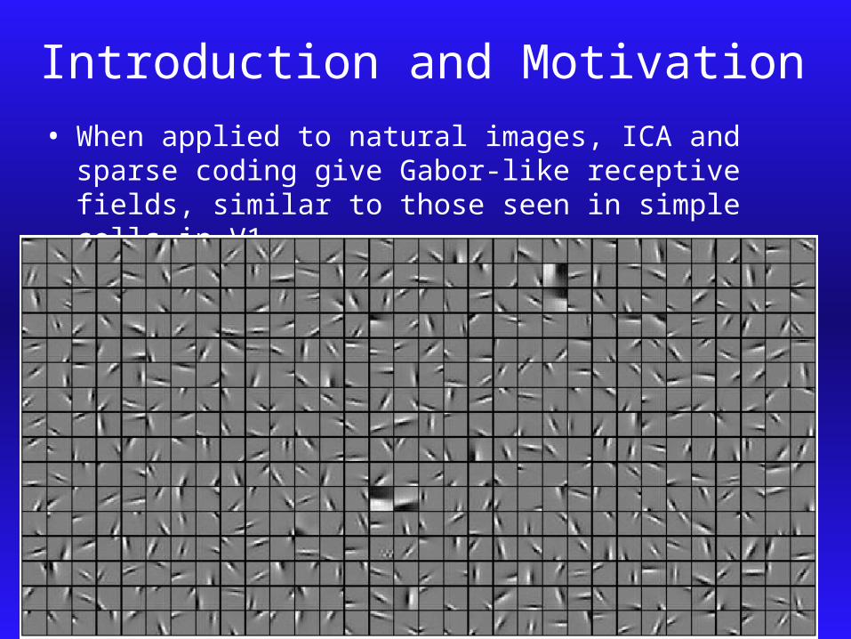
Introduction and Motivation• When applied to natural images, ICA and sparse
coding give Gabor-like receptive fields, similar to those seen in simple cells in V1
Introduction and Motivation
• There have been many attempts to go beyond a single layer (Karklin, Y., & Lewicki, M. S. (2006), Schwartz, O., & Simoncelli, E. P. (2001) Hoyer & Hyvarinen
(2002) but:• They usually require a different learning rule
• And do not lead to a way to do the next layer.
• Or, like deep belief networks, do not have plausible receptive fields (Hinton, 2006)
Our contribution• We have previously developed a method for
applying ICA over and over, in order to get higher layer representations (Shan, Zhang, & Cottrell, NIPS, 2006/2007), called RICA
• Recursive Independent Components Analysis:
ICA->add nonlinearity->ICA->add nonlinearity…
• In our paper, we showed that the second layer of ICA had interesting neural properties
Roadmap• We describe ICA and our version of a hierarchical
ICA, Recursive ICA (RICA)
• We illustrate PCA and describe sparse PCA (SPCA) and the initial results
• We investigate the receptive fields of the higher layers of RICA.
Roadmap• We describe ICA and our version of a
hierarchical ICA, Recursive ICA (RICA)
• We illustrate PCA and describe sparse PCA (SPCA) and the initial results
• We investigate the receptive fields of the higher layers of RICA.
Independent Components Analysis
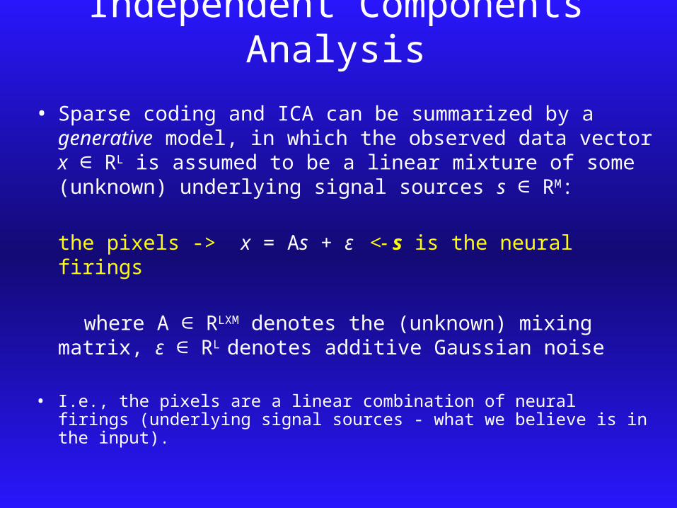
• Sparse coding and ICA can be summarized by a generative model, in which the observed data vector x ∈ RL is assumed to be a linear mixture of some (unknown) underlying signal sources s ∈ RM:
the pixels -> x = As + ε <- s is the neural firings
where A ∈ RLXM denotes the (unknown) mixing matrix, ε ∈ RL denotes additive Gaussian noise
• I.e., the pixels are a linear combination of neural firings (underlying signal sources - what we believe is in the input).

Independent Components Analysis
x = As + ε
• Two assumptions are imposed on the signal sources:1.They are assumed to be independent2.Each dimension of s is assumed to follow a
sparse distribution, usually with a peak at zero and two heavy tails, unlike PCA, where the projections tend to follow a Gaussian.
• Model parameters are adapted to make the generation of the observed x’s likely, and to encourage the sparse prior:
Recursive Independent Components Analysis (RICA 1.0)
• We assume that higher layers of cortex follow a similar learning rule as earlier layers - so we would like to apply essentially the same learning rule to subsequent layers.
• BUT:• More linear processing will not lead to
more interesting structure…• So we need some nonlinearity applied to
the output of the first layer of ICA…

Recursive Independent Components Analysis (RICA 1.0)• Notice that the generative model:
x = As + ε
• means that:
xi= j Aij*sj + εi
• Thus, each input variable (pixel) is assumed to be the sum of many independent random variables…
Recursive Independent Components Analysis (RICA 1.0)
• Thus, each input variable (pixel) is assumed to be the sum of many independent random variables…
i.e., it follows a Gaussian distribution!
Idea: ICA therefore expects a Gaussian distributed input - which makes applying a second layer of ICA to a sparsely distributed input unlikely to work well.
Hence, we apply a component-wise nonlinearity to the first layer outputs to make the output follow a Gaussian distribution.

Recursive Independent Components Analysis (RICA 1.0)• Another observation: The sign of the output of any si is
redundant statistically:
This is the distribution of one signal source (s2) as a function of the value of a neighboring signal source (s1) …

Recursive Independent Components Analysis (RICA 1.0)• Hence our nonlinear activation function:
• Note that ambiguous (not quite on, not quite off) responses (in BLUE) are emphasized in the activation function

Recursive Independent Components Analysis (RICA 1.0)
• An actual nonlinear activation function

Recursive Independent Components Analysis (RICA 1.0)
• We applied RICA 1.0 to natural image patches.
• Layer-1 ICA learns the standard edge/bar shaped visual features.
• Layer-2 ICA learns more complex visual features that appear to capture contour and texture (Shan, Zhang & Cottrell, NIPS, 2007).
QuickTime™ and a decompressor
are needed to see this picture.

Recursive Independent Components Analysis (RICA 1.0)
Furthermore, these nonlinear features are useful:
• We applied layer 1 features with the nonlinearity to face recognition, and obtained state-of-the-art recognition performance on face recognition, using a simple linear classifier (Shan & Cottrell, CVPR, 2008).
• We also used the layer 1 features in a completely different recognition system we applied to faces, objects and flowers, and got state-of-the-art results on all three, without retraining (Kanan & Cottrell, CVPR, 2010)

Results (NIPS 06/07)• Error rates on the Yale face database:
Number of training examples
QuickTime™ and a decompressor
are needed to see this picture.
Nu
mb
er
of
featu
res

CVPR 2010
• Both the salience map and the features stored at each location are ICA features with our nonlinearity
Image Fixate Region
Local Features
Decide where to look
LocalClassifier
Decision?
Get next fixation?

Improvement Over State-of-the-art

Improvement Over State-of-the-art
Roadmap• We describe ICA and our version of a hierarchical
ICA, Recursive ICA (RICA 1.0)
• We illustrate PCA and describe sparse PCA (SPCA) and the initial results
• We investigate the receptive fields of the higher layers of RICA 2.0.

The “hidden layers”• The story I told:
• Recursive Independent Components Analysis:
ICA->add nonlinearity->ICA->add nonlinearity…
• The truth: in fact, like everyone else who does this sort of work, it is actually interleaved with PCA:
• PCA->ICA->add nonlinearity->PCA->ICA->add nonlinearity…
• And like everyone else, we never publish the pictures of the PCA receptive fields - because they don’t look biologically plausible!
RICA 2.0
• We now combine this with our improvements to sparse PCA (Vincent et al., 2005) to get receptive fields up to V2.
• SPCA->ICA->add nonlinearity->SPCA->ICA->add nonlinearity…
• And, sparse PCA learns biologically-realistic receptive fields.

A simple (unrealistic) example• Suppose two input signals (e.g., pixels) are completely
correlated:
Pixel 1
Pixel 2
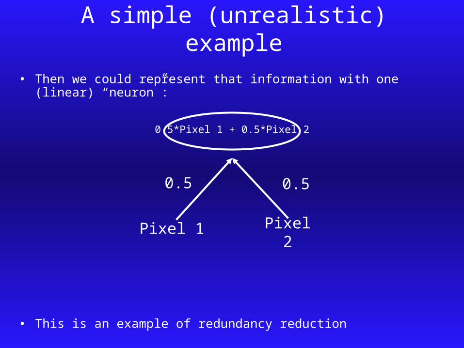
A simple (unrealistic) example• Then we could represent that information with one (linear)
“neuron”:
• This is an example of redundancy reduction
Pixel 1 Pixel 2
0.5 0.5
0.5*Pixel 1 + 0.5*Pixel 2

A simple (unrealistic) example• Furthermore, we can reconstruct the original pixels from that
one “neural response”:
0.5*Pixel 1 + 0.5*Pixel 2
Pixel 1 Pixel 2
1.0 1.0
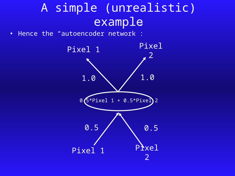
A simple (unrealistic) example• Hence the “autoencoder network”:
Pixel 1 Pixel 2
0.5 0.5
0.5*Pixel 1 + 0.5*Pixel 2
Pixel 1 Pixel 2
1.0 1.0

Principal Components Analysis
• Principal Components Analysis would do exactly this, because it learns representations based on correlations between the inputs.
• This is an example of redundancy reduction and dimensionality reduction (from 2 dimensions to 1)
Pixel 1 Pixel 2
0.5 0.5
0.5*Pixel 1 + 0.5*Pixel 2

Principal Components Analysis
• Note that we can plot this “principal component” in image space, corresponding to the “weights”, (0.5,0.5)
• The same thing applies if we have more than two pixels…so we have more than 2 principal components…capturing more correlations…
Pixel 1 Pixel 2
0.5 0.5
0.5*Pixel 1 + 0.5*Pixel 2
Pixel 1 Pixel 2

Principal Components Analysis
• And now we can see that the reconstruction is a weighted version of that “image”
• The same thing applies if we have more than two pixels…so we have more than 2 principal components…capturing more correlations…
0.5*Pixel 1 + 0.5*Pixel 2
Pixel 1 Pixel 2
1.0 1.0Pixel 1 Pixel
2

Principal Components Analysis
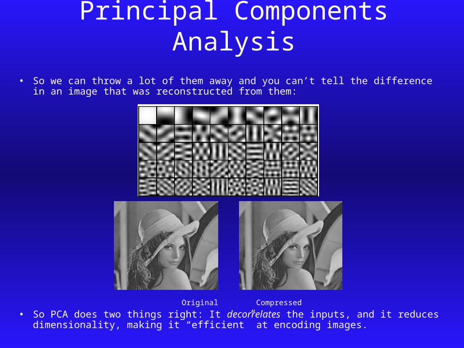
• Here are the principal components of 10x10 patches of natural images:

Principal Components Analysis
• But PCA learns these correlations in order of their size: so the first principal component does a lot of work:
1st PC

Principal Components Analysis
• and the last principal component does very little work:
last PC
Principal Components Analysis
• So we can throw a lot of them away and you can’t tell the difference in an image that was reconstructed from them:
Original Compressed
• So PCA does two things right: It decorrelates the inputs, and it reduces dimensionality, making it “efficient” at encoding images.

Principal Components Analysis
• But no neuron should have to be the first principal component: So we should distribute the load evenly - this is called “response equalization.”

Principal Components Analysis
• Secondly, PCA is profligate with connections - every pixel is connected to every principal component “neuron”: we should try to reduce the connections also.
Sparse Principal Components Analysis
• We will try to minimize reconstruction error,
• While trying to equalize the neural responses
• And minimizing the connections.

• We minimize:
• Subject to the following constraint:
Sparse Principal Components Analysis
Reconstructionerror Minimize
connections
Equalize the “work”

Information Kept With Sparse Connections
• We applied the model to 20 X 20 image patches, and reduced the dimensionality to 100.
• Results:
• Our model captures 99.23% of the variance that could be captured by PCA with 100 output neurons.
• 96.31% of the connection weights in our model are zero.

Information Kept With Sparse Connections
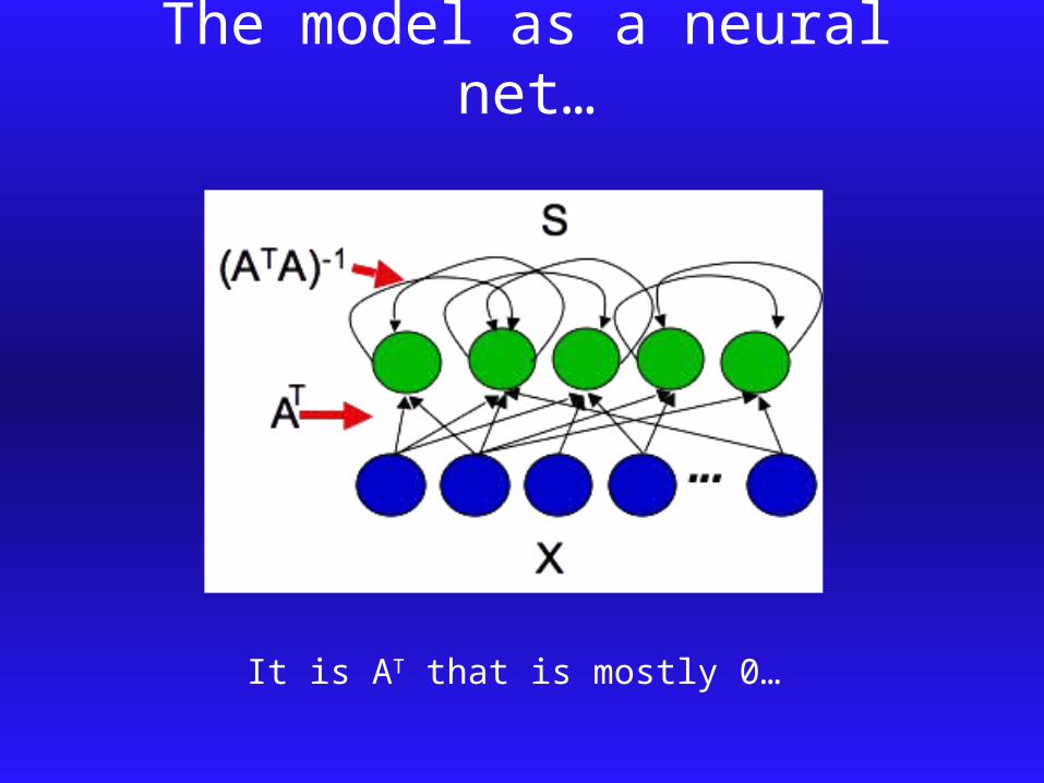
The model as a neural net…
It is AT that is mostly 0…
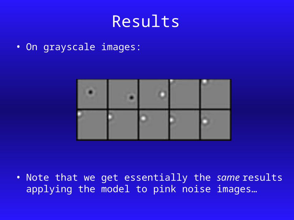
Results• On grayscale images:
• Note that we get essentially the same results applying the model to pink noise images…

Results
• suggesting the 1/f power spectrum of images is where this is coming from…

Results• On color images:
• Many people have gotten this color opponency before, but not in center-surround shape.

Results• The role of the number of features: 100 versus 32

Results• The role of :
• Recall this reduces the number of connections…

Results• The role of : higher means
fewer connections, which alters the contrast sensitivity function (CSF).
• Matches recent data on malnourished kids and their CSF’s: lower sensitivity at low spatial frequencies, but slightly better at high than normal controls…

Trained on grayscale video…
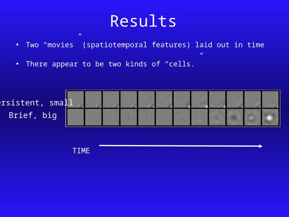
Results• Two “movies” (spatiotemporal features) laid out in time • There appear to be two kinds of “cells.”
TIME
Persistent, small
Brief, big

Midget?
Parasol?
This suggests that these cell types exist because they
are useful for efficiently encoding the temporal dynamics of the world.
Persistent, small
Brief, big

Roadmap• We describe ICA and our version of a hierarchical
ICA, Recursive ICA (RICA 1.0)
• We illustrate PCA and describe sparse PCA (SPCA) and the initial results
• We investigate the receptive fields of the higher layers of RICA 2.0.

Recursive Independent Components Analysis (RICA 1.0)While in this talk, we only go as far as layer 2,
obviously, we could keep going.
Our goal is to check whether we are consistent with the neurophysiology before continuing.
Enter Sparse PCA:
RICA 2.0=RICA 1.0 + Sparse PCA
• Now, we no longer have to hide the PCA results!
• Question: What happens when we apply sparse PCA to the (nonlinearized) ICA outputs of the first layer??
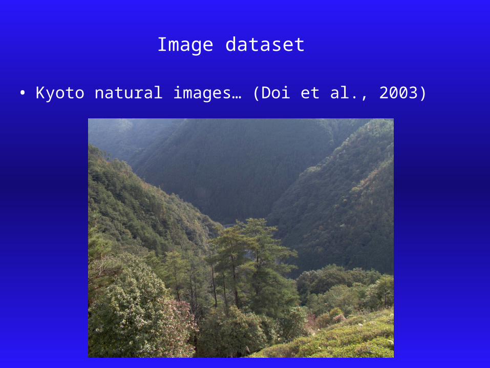
Image dataset
• Kyoto natural images… (Doi et al., 2003)
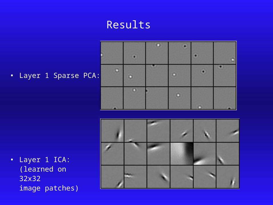
Results
• Layer 1 Sparse PCA:
• Layer 1 ICA:(learned on 32x32 image patches)
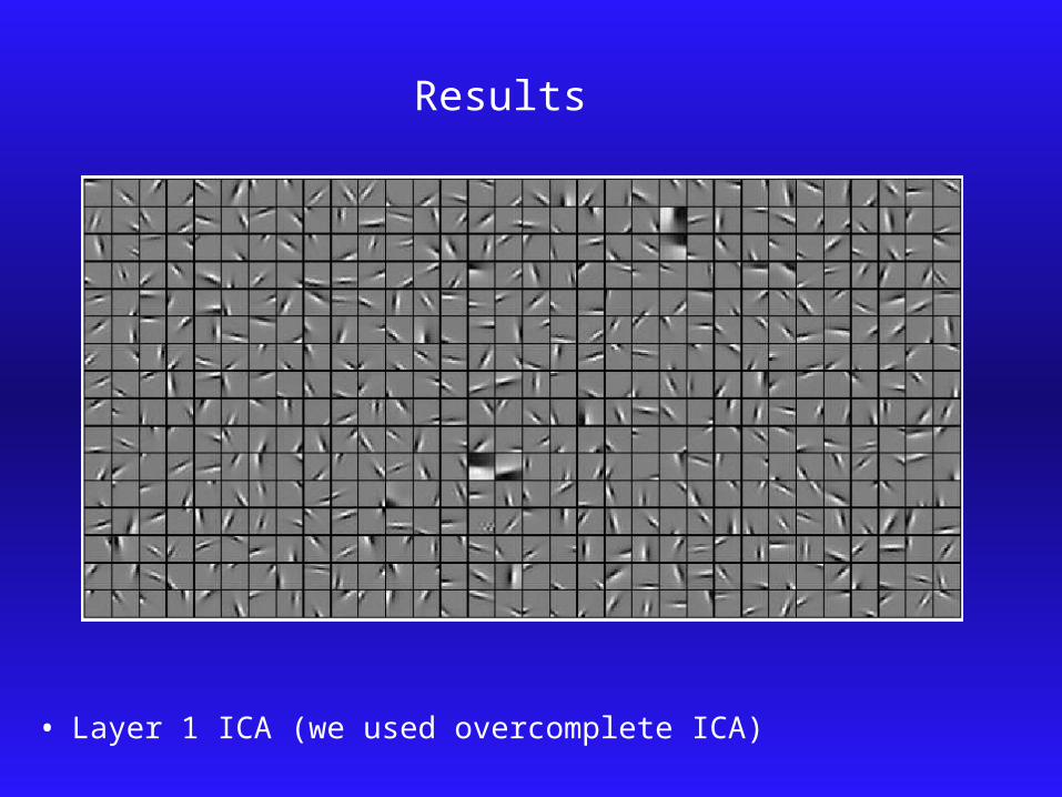
Results
• Layer 1 ICA (we used overcomplete ICA)
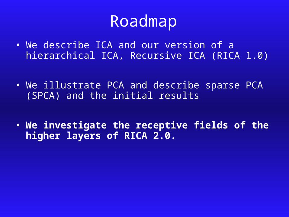
Roadmap• We describe ICA and our version of a hierarchical
ICA, Recursive ICA (RICA 1.0)
• We illustrate PCA and describe sparse PCA (SPCA) and the initial results
• We investigate the receptive fields of the higher layers of RICA 2.0.

Visualization• We take these:
• And fit gabor filters to them, and then plot them on on top of one anothertop of one another showing the major axis
• Then we color them by the strength of connections to them by the next layer - to show a receptive field.

Layer 2 Sparse PCA cells
• Each patch represents one layer-2 PCA feature. • Within the patch, each bar represents one layer-1 ICA feature.
• The layer-1 ICA features are fitted to Gabor kernel functions.
• The locations, orientations, lengths of the bars represent the locations,
orientations, frequencies of the fitted Gabor functions.
• The colors of the bars represent the connection strengths from the layer-2
PCA feature to the layer-1 ICA features. • Warm colors represent positive connections; Cold colors represent negative
connections; Gray colors represent connection strengths that are close to zero.

Layer 2 Sparse PCA cells
• A positive connection suggests that this layer-2 PCA features prefers strong
responses, either positive or negative, from that layer-1 ICA feature.
• A negative connection suggests that it prefers weak or no responses from
that layer-1 ICA feature.
• These perform the pooling operation on V1 simple cell responses: I.e., they
agree with complex cell responses - but they also represent “OFF”-pooling
responses (the cold colors)

Layer 2 ICA features
• Unlike previous visual layers, there isn’t a general consensus about the visual features captured by V2 cells.
• We choose to compare our learned features with (Anzai, Peng, & Van Essen, Nature Neuroscience, 2007), because
(1)(1) It is a recent result, so they may reflect the most It is a recent result, so they may reflect the most recent views about V2 cells from experimental recent views about V2 cells from experimental neuroscience; neuroscience;
(2)(2) They adopted a similar technique as how we visualize They adopted a similar technique as how we visualize the second layer features to describe the V2 cells’ the second layer features to describe the V2 cells’ receptive fields, hence it is convenient to compare our receptive fields, hence it is convenient to compare our results with their results.results with their results.

Layer 2 ICA features
• They recorded 136 V2 cells from 16 macaque monkeys, but only reported the results on 118 of them (we will go back to this point later!!!)
• For each V2 cell, they first identified its classical receptive fields. Then they displayed 19 bars arranged in hexagonal arrays within the receptive field, whose sizes are much smaller than the receptive field size.
• They varied the orientations of the bars, and measured the V2 neurons’ responses to those settings.
• In the end, they got a space-orientation RF map for each V2 neuron.

Layer 2 ICA features
• In the end, they got a space-orientation RF map for each V2 neuron.
• The first shows uniform orientation tuning across its receptive field; the second, non-uniform tuning in different sub-regions of space.

Layer 2 ICA features
The left-most column displays two model neurons that show uniform orientation preference to layer-1 ICA features.
The middle column displays model neurons that have non-uniform/varying orientation preference to layer-1 ICA features. The right column displays two model neurons that have location preference, but no orientation preference, to layer-1 ICA features.
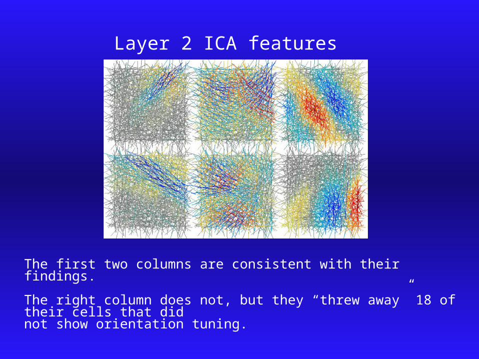
Layer 2 ICA features
The first two columns are consistent with their findings. The right column does not, but they “threw away” 18 of their cells that did not show orientation tuning.

Summary• Dimensionality Reduction (e.g., Sparse PCA) &
Expansion (e.g., overcomplete ICA) might be a general strategy of information processing in the brain.
• The first step removes noise and reduces complexity, the second step captures the statistical structure.
• We showed that retinal ganglion cells and V1 complex cells may be derived from the same learning algorithm, applied to pixels in one case, and V1 simple cell outputs in the second.
• This highly simplified model of early vision is the first one that learns the RFs of all early visual layers, using a consistent theory - the efficient coding theory.
• We believe it could serve as a basis for more sophisticated models of early vision.

END