(e book) wiley & sons 4g wireless video communications (2009)
TRANSCRIPT


4G WIRELESS VIDEOCOMMUNICATIONS
4G Wireless Video Communications Haohong Wang, Lisimachos P. Kondi, Ajay Luthra and Song Ci
© 2009 John Wiley & Sons, Ltd. ISBN: 978-0-470-77307-9

Wiley Series on Wireless Communications and Mobile Computing
Series Editors: Dr Xuemin (Sherman) Shen, University of Waterloo, Canada
Dr Yi Pan, Georgia State University, USA
The “Wiley Series on Wireless Communications and Mobile Computing” is a series of comprehensive, practical
and timely books on wireless communication and network systems. The series focuses on topics ranging from
wireless communication and coding theory to wireless applications and pervasive computing. The books provide
engineers and other technical professionals, researchers, educators, and advanced students in these fields with
invaluable insight into the latest developments and cutting-edge research.
Other titles in the series:
Misic and Misic: Wireless Personal Area Networks: Performance, Interconnection, and Security with IEEE 802.15.4 ,
January 2008, 978-0-470-51847-2
Takagi and Walke: Spectrum Requirement Planning in Wireless Communications: Model and Methodology for
IMT-Advanced , April 2008, 978-0-470-98647-9
Perez-Fontan and Espineira: Modeling the Wireless Propagation Channel: A simulation approach with MATLAB,
August 2008, 978-0-470-72785-0
Ippolito: Satellite Communications Systems Engineering: Atmospheric Effects, Satellite Link Design and System
Performance, August 2008, 978-0-470-72527-6
Lin and Sou: Charging for Mobile All-IP Telecommunications , September 2008, 978-0-470-77565-3
Myung and Goodman: Single Carrier FDMA: A New Air Interface for Long Term Evolution, October 2008,
978-0-470-72449-1
Hart, Tao and Zhou: Mobile Multi-hop WiMAX: From Protocol to Performance, July 2009, 978-0-470-99399-6
Cai, Shen and Mark: Multimedia Services in Wireless Internet: Modeling and Analysis , August 2009,
978-0-470-77065-8
Stojmenovic: Wireless Sensor and Actuator Networks: Algorithms and Protocols for Scalable Coordination and
Data Communication, September 2009, 978-0-470-17082-3
Qian, Muller and Chen: Security in Wireless Networks and Systems , January 2010, 978-0-470-51212-8

4G WIRELESS VIDEOCOMMUNICATIONS
Haohong Wang
Marvell Semiconductors, USA
Lisimachos P. Kondi
University of Ioannina, Greece
Ajay Luthra
Motorola, USA
Song Ci
University of Nebraska-Lincoln, USA
A John Wiley and Sons, Ltd., Publication

This edition first published 2009
2009, John Wiley & Sons Ltd.,
Registered office
John Wiley & Sons, Ltd, The Atrium, Southern Gate, Chichester, West Sussex PO19 8SQ, United Kingdom
For details of our global editorial offices, for customer services and for information about how to apply for
permission to reuse the copyright material in this book please see our website at www.wiley.com.
The right of the author to be identified as the author of this work has been asserted in accordance with the
Copyright, Designs and Patents Act 1988.
All rights reserved. No part of this publication may be reproduced, stored in a retrieval system, or transmitted, in
any form or by any means, electronic, mechanical, photocopying, recording or otherwise, except as permitted by
the UK Copyright, Designs and Patents Act 1988, without the prior permission of the publisher.
Wiley also publishes its books in a variety of electronic formats. Some content that appears in print may not be
available in electronic books.
Designations used by companies to distinguish their products are often claimed as trademarks. All brand names
and product names used in this book are trade names, service marks, trademarks or registered trademarks of
their respective owners. The publisher is not associated with any product or vendor mentioned in this book. This
publication is designed to provide accurate and authoritative information in regard to the subject matter covered.
It is sold on the understanding that the publisher is not engaged in rendering professional services. If professional
advice or other expert assistance is required, the services of a competent professional should be sought.
Library of Congress Cataloging-in-Publication Data:
4G wireless video communications / Haohong Wang . . . [et al.].
p. cm.
Includes bibliographical references and index.
ISBN 978-0-470-77307-9 (cloth)
1. Multimedia communications. 2. Wireless communication systems. 3. Video
telephone. I. Wang, Haohong, 1973-
TK5105.15.A23 2009
621.384 – dc22
2008052216
A catalogue record for this book is available from the British Library.
ISBN 978-0-470-77307-9 (H/B)
Typeset in 10/12pt Times by Laserwords Private Limited, Chennai, India.
Printed and bound in Great Britain by Antony Rowe Ltd, Chippenham, Wiltshire.

Contents
Foreword xiii
Preface xv
About the Authors xxi
About the Series Editors xxv
1 Introduction 1
1.1 Why 4G? 1
1.2 4G Status and Key Technologies 3
1.2.1 3GPP LTE 3
1.2.2 Mobile WiMAX 4
1.3 Video Over Wireless 5
1.3.1 Video Compression Basics 5
1.3.2 Video Coding Standards 9
1.3.3 Error Resilience 10
1.3.4 Network Integration 12
1.3.5 Cross-Layer Design for Wireless Video Delivery 14
1.4 Challenges and Opportunities for 4G Wireless Video 15
References 17
2 Wireless Communications and Networking 19
2.1 Characteristics and Modeling of Wireless Channels 19
2.1.1 Degradation in Radio Propagation 19
2.1.2 Rayleigh Fading Channel 20
2.2 Adaptive Modulation and Coding 23
2.2.1 Basics of Modulation Schemes 23
2.2.2 System Model of AMC 25
2.2.3 Channel Quality Estimation and Prediction 26
2.2.4 Modulation and Coding Parameter Adaptation 28

vi Contents
2.2.5 Estimation Error and Delay in AMC 30
2.2.6 Selection of Adaptation Interval 30
2.3 Orthogonal Frequency Division Multiplexing 31
2.3.1 Background 31
2.3.2 System Model and Implementation 31
2.3.3 Pros and Cons 33
2.4 Multiple-Input Multiple-Output Systems 34
2.4.1 MIMO System Model 34
2.4.2 MIMO Capacity Gain: Multiplexing 35
2.4.3 MIMO Diversity Gain: Beamforming 35
2.4.4 Diversity-Multiplexing Trade-offs 35
2.4.5 Space-Time Coding 36
2.5 Cross-Layer Design of AMC and HARQ 37
2.5.1 Background 38
2.5.2 System Modeling 39
2.5.3 Cross-Layer Design 41
2.5.4 Performance Analysis 44
2.5.5 Performance 45
2.6 Wireless Networking 47
2.6.1 Layering Network Architectures 48
2.6.2 Network Service Models 50
2.6.3 Multiplexing Methods 51
2.6.4 Connection Management in IP-Based Data Networks 53
2.6.5 QoS Handoff 54
2.7 Summary 55
References 56
3 Video Coding and Communications 59
3.1 Digital Video Compression – Why and How Much? 59
3.2 Basics 60
3.2.1 Video Formats 60
3.2.1.1 Scanning 60
3.2.1.2 Color 61
3.2.1.3 Luminance, Luma, Chrominance, Chroma 64
3.3 Information Theory 64
3.3.1 Entropy and Mutual Information 65
3.3.2 Encoding of an Information Source 66
3.3.3 Variable Length Coding 68
3.3.4 Quantization 71
3.4 Encoder Architectures 73
3.4.1 DPCM 73
3.4.2 Hybrid Transform-DPCM Architecture 77
3.4.3 A Typical Hybrid Transform DPCM-based Video Codec 79
3.4.4 Motion Compensation 82
3.4.5 DCT and Quantization 83
3.4.6 Procedures Performed at the Decoder 84

Contents vii
3.5 Wavelet-Based Video Compression 86
3.5.1 Motion-Compensated Temporal Wavelet Transform Using Lifting 90
References 94
4 4G Wireless Communications and Networking 97
4.1 IMT-Advanced and 4G 97
4.2 LTE 99
4.2.1 Introduction 101
4.2.2 Protocol Architecture 102
4.2.2.1 E-UTRAN Overview Architecture 102
4.2.2.2 User Plane and Control Plane 102
4.2.2.3 LTE Physical Layer 106
4.2.3 LTE Layer 2 107
4.2.4 The Evolution of Architecture 110
4.2.5 LTE Standardization 110
4.3 WIMAX-IEEE 802.16m 112
4.3.1 Network Architecture 113
4.3.2 System Reference Model 114
4.3.3 Protocol Structure 114
4.3.3.1 MAC Layer 114
4.3.3.2 PHY Layer 120
4.3.4 Other Functions Supported by IEEE 802.16m for Further Study 125
4.4 3GPP2 UMB 125
4.4.1 Architecture Reference Model 126
4.4.2 Layering Architecture and Protocols 127
Acknowledgements 133
References 133
5 Advanced Video Coding (AVC)/H.264 Standard 135
5.1 Digital Video Compression Standards 135
5.2 AVC/H.264 Coding Algorithm 138
5.2.1 Temporal Prediction 139
5.2.1.1 Motion Estimation 140
5.2.1.2 P and B MBs 142
5.2.1.3 Multiple References 143
5.2.1.4 Motion Estimation Accuracy 143
5.2.1.5 Weighted Prediction 144
5.2.1.6 Frame and Field MV 144
5.2.1.7 MV Compression 145
5.2.2 Spatial Prediction 147
5.2.3 The Transform 148
5.2.3.1 4 × 4 Integer DCT and Inverse Integer DCT Transform 149
5.2.3.2 8 × 8 Transform 150
5.2.3.3 Hadamard Transform for DC 151

viii Contents
5.2.4 Quantization and Scaling 151
5.2.5 Scanning 151
5.2.6 Variable Length Lossless Codecs 152
5.2.6.1 Exp-Golomb Code 153
5.2.6.2 CAVLC (Context Adaptive VLC) 154
5.2.6.3 CABAC 154
5.2.7 Deblocking Filter 155
5.2.8 Hierarchy in the Coded Video 156
5.2.8.1 Basic Picture Types (I, P, B, BR) 157
5.2.8.2 SP and SI Pictures 157
5.2.9 Buffers 158
5.2.10 Encapsulation/Packetization 159
5.2.11 Profiles 160
5.2.11.1 Baseline Profile 160
5.2.11.2 Extended Profile 162
5.2.11.3 Main Profile 162
5.2.11.4 High Profile 162
5.2.11.5 High10 Profile 163
5.2.11.6 High 4:2:2 Profile 163
5.2.11.7 High 4:4:4 Predictive Profile 163
5.2.11.8 Intra Only Profiles 163
5.2.12 Levels 163
5.2.12.1 Maximum Bit Rates, Picture Sizes and Frame Rates 164
5.2.12.2 Maximum CPB, DPB and Reference Frames 164
5.2.13 Parameter Sets 167
5.2.13.1 Sequence Parameter Sets (SPS) 167
5.2.13.2 Picture Parameter Sets (PPS) 167
5.2.14 Supplemental Enhancement Information (SEI) 167
5.2.15 Subjective Tests 168
References 168
6 Content Analysis for Communications 171
6.1 Introduction 171
6.2 Content Analysis 173
6.2.1 Low-Level Feature Extraction 174
6.2.1.1 Edge 174
6.2.1.2 Shape 176
6.2.1.3 Color 177
6.2.1.4 Texture 177
6.2.1.5 Motion 178
6.2.1.6 Mathematical Morphology 178
6.2.2 Image Segmentation 179
6.2.2.1 Threshold and Boundary Based Segmentation 181
6.2.2.2 Clustering Based Segmentation 181
6.2.2.3 Region Based Approach 181
6.2.2.4 Adaptive Perceptual Color-Texture Segmentation 182

Contents ix
6.2.3 Video Object Segmentation 185
6.2.3.1 COST211 Analysis Model 187
6.2.3.2 Spatial-Temporal Segmentation 187
6.2.3.3 Moving Object Tracking 188
6.2.3.4 Head-and-Shoulder Object Segmentation 190
6.2.4 Video Structure Understanding 200
6.2.4.1 Video Abstraction 201
6.2.4.2 Video Summary Extraction 203
6.2.5 Analysis Methods in Compressed Domain 208
6.3 Content-Based Video Representation 209
6.4 Content-Based Video Coding and Communications 212
6.4.1 Object-Based Video Coding 212
6.4.2 Error Resilience for Object-Based Video 215
6.5 Content Description and Management 217
6.5.1 MPEG-7 217
6.5.2 MPEG-21 219
References 219
7 Video Error Resilience and Error Concealment 223
7.1 Introduction 223
7.2 Error Resilience 224
7.2.1 Resynchronization Markers 224
7.2.2 Reversible Variable Length Coding (RVLC) 225
7.2.3 Error-Resilient Entropy Coding (EREC) 226
7.2.4 Independent Segment Decoding 228
7.2.5 Insertion of Intra Blocks or Frames 228
7.2.6 Scalable Coding 229
7.2.7 Multiple Description Coding 230
7.3 Channel Coding 232
7.4 Error Concealment 234
7.4.1 Intra Error Concealment Techniques 234
7.4.2 Inter Error Concealment Techniques 234
7.5 Error Resilience Features of H.264/AVC 236
7.5.1 Picture Segmentation 236
7.5.2 Intra Placement 236
7.5.3 Reference Picture Selection 237
7.5.4 Data Partitioning 237
7.5.5 Parameter Sets 237
7.5.6 Flexible Macroblock Ordering 238
7.5.7 Redundant Slices (RSs) 239
References 239
8 Cross-Layer Optimized Video Delivery over 4G Wireless Networks 241
8.1 Why Cross-Layer Design? 241
8.2 Quality-Driven Cross-Layer Framework 242

x Contents
8.3 Application Layer 244
8.4 Rate Control at the Transport Layer 244
8.4.1 Background 244
8.4.2 System Model 246
8.4.3 Network Setting 246
8.4.4 Problem Formulation 248
8.4.5 Problem Solution 248
8.4.6 Performance Evaluation 249
8.5 Routing at the Network Layer 252
8.5.1 Background 252
8.5.2 System Model 254
8.5.3 Routing Metric 255
8.5.4 Problem Formulation 257
8.5.5 Problem Solution 258
8.5.6 Implementation Considerations 262
8.5.7 Performance Evaluation 263
8.6 Content-Aware Real-Time Video Streaming 265
8.6.1 Background 265
8.6.2 Background 265
8.6.3 Problem Formulation 266
8.6.4 Routing Based on Priority Queuing 267
8.6.5 Problem Solution 269
8.6.6 Performance Evaluation 270
8.7 Cross-Layer Optimization for Video Summary Transmission 272
8.7.1 Background 272
8.7.2 Problem Formulation 274
8.7.3 System Model 276
8.7.4 Link Adaptation for Good Content Coverage 278
8.7.5 Problem Solution 280
8.7.6 Performance Evaluation 283
8.8 Conclusions 287
References 287
9 Content-based Video Communications 291
9.1 Network-Adaptive Video Object Encoding 291
9.2 Joint Source Coding and Unequal Error Protection 294
9.2.1 Problem Formulation 295
9.2.1.1 System Model 296
9.2.1.2 Channel Model 297
9.2.1.3 Expected Distortion 298
9.2.1.4 Optimization Formulation 298
9.2.2 Solution and Implementation Details 299
9.2.2.1 Packetization and Error Concealment 299
9.2.2.2 Expected Distortion 299
9.2.2.3 Optimal Solution 300
9.2.3 Application on Energy-Efficient Wireless Network 301

Contents xi
9.2.3.1 Channel Model 301
9.2.3.2 Experimental Results 302
9.2.4 Application on Differentiated Services Networks 303
9.3 Joint Source-Channel Coding with Utilization of Data Hiding 305
9.3.1 Hiding Shape in Texture 308
9.3.2 Joint Source-Channel Coding 309
9.3.3 Joint Source-Channel Coding and Data Hiding 311
9.3.3.1 System Model 311
9.3.3.2 Channel Model 312
9.3.3.3 Expected Distortion 312
9.3.3.4 Implementation Details 313
9.3.4 Experimental Results 315
References 322
10 AVC/H.264 Application – Digital TV 325
10.1 Introduction 325
10.1.1 Encoder Flexibility 326
10.2 Random Access 326
10.2.1 GOP Bazaar 327
10.2.1.1 MPEG-2 Like, 2B, GOP Structure 327
10.2.1.2 Reference B and Hierarchical GOP structures 330
10.2.1.3 Low Delay Structure 331
10.2.1.4 Editable Structure 331
10.2.1.5 Others 332
10.2.2 Buffers, Before and After 332
10.2.2.1 Coded Picture Buffer 332
10.2.2.2 Decoded Picture Buffer (DPB) 334
10.3 Bitstream Splicing 335
10.4 Trick Modes 337
10.4.1 Fast Forward 338
10.4.2 Reverse 338
10.4.3 Pause 338
10.5 Carriage of AVC/H.264 Over MPEG-2 Systems 338
10.5.1 Packetization 339
10.5.1.1 Packetized Elementary Stream (PES) 340
10.5.1.2 Transport Stream (TS) 340
10.5.1.3 Program Stream 343
10.5.2 Audio Video Synchronization 344
10.5.3 Transmitter and Receiver Clock Synchronization 344
10.5.4 System Target Decoder and Timing Model 344
References 345
11 Interactive Video Communications 347
11.1 Video Conferencing and Telephony 347
11.1.1 IP and Broadband Video Telephony 347

xii Contents
11.1.2 Wireless Video Telephony 348
11.1.3 3G-324M Protocol 348
11.1.3.1 Multiplexing and Error Handling 349
11.1.3.2 Adaptation Layers 350
11.1.3.3 The Control Channel 350
11.1.3.4 Audio and Video Channels 350
11.1.3.5 Call Setup 350
11.2 Region-of-Interest Video Communications 351
11.2.1 ROI based Bit Allocation 351
11.2.1.1 Quality Metric for ROI Video 351
11.2.1.2 Bit Allocation Scheme for ROI Video 353
11.2.1.3 Bit Allocation Models 354
11.2.2 Content Adaptive Background Skipping 356
11.2.2.1 Content-based Skip Mode Decision 357
11.2.2.2 ρ Budget Adjustment 360
References 366
12 Wireless Video Streaming 369
12.1 Introduction 369
12.2 Streaming System Architecture 370
12.2.1 Video Compression 370
12.2.2 Application Layer QoS Control 372
12.2.2.1 Rate Control 372
12.2.2.2 Rate Shaping 373
12.2.2.3 Error Control 374
12.2.3 Protocols 374
12.2.3.1 Transport Protocols 375
12.2.4 Video/Audio Synchronization 376
12.3 Delay-Constrained Retransmission 377
12.3.1 Receiver-Based Control 378
12.3.2 Sender-Based Control 378
12.3.3 Hybrid Control 379
12.3.4 Rate-Distortion Optimal Retransmission 379
12.4 Considerations for Wireless Video Streaming 382
12.4.1 Cross-Layer Optimization and Physical Layer Consideration 383
12.5 P2P Video Streaming 384
References 385
Index 389

Foreword
4G Wireless Video Communications is a broad title with a wide scope, bridging video
signal processing, video communications, and 4G wireless networks. Currently, 4G wire-
less communication systems are still in their planning phase. The new infrastructure is
expected to provide much higher data rates, lower cost per transmitted bit, more flexible
mobile terminals, and seamless connections to different networks. Along with the rapid
development of video coding and communications techniques, more and more advanced
interactive multimedia applications are emerging as 4G network “killer apps”.
Depending on the reader’s background and point of view, this topic may be considered
and interpreted with different perspectives and foci. Colleagues in the multimedia signal
processing area know firsthand the effort and ingenuity it takes to save 1 bit or increase
the quality of the reconstructed video during compression by 0.5 dB. The increased band-
width of 4G systems may open the door to new challenges and open issues that will
be encountered for first time or were neglected before. Some topics, such as content
interactivity, scalability, and understandability may be reconsidered and be given higher
priority, and a more aggressive approach in investigating and creating new applications
and service concepts may be adopted. On the other hand, for colleagues with communica-
tions and networking backgrounds, it is important to keep in mind that in the multimedia
content delivery scenario, every bit or packet is not equal from the perspective of power
consumption, delay, or packet loss. In other words, media data with certain semantic and
syntactical characteristics may impact the resulting user experience more significantly than
others. Therefore it is critical to factor this in to the design of new systems, protocols, and
algorithms. Consequently, the cross-layer design and optimization for 4G wireless video
is expected to be an active topic. It will gather researchers from various communities
resulting in necessary inter-disciplinary collaborations.
In this book, the authors have successfully provided a detailed coverage of the funda-
mental theory of video compression, communications, and 4G wireless communications.
A comprehensive treatment of advanced video analysis and coding techniques, as well as
the new emerging techniques and applications, is also provided. So far, to the best of my
knowledge, I have seen very few books, journals or magazines on the market focusing
on this topic, which may be due to the very fast developments in this field. This book
has revealed an integrated picture of 4G wireless video communications to the general
audience. It provides both a treatment of the underlying theory and a valuable practical
reference for the multimedia and communications practitioners.
Aggelos K. Katsaggelos
Professor of Electrical Engineering and Computer Science
Northwestern University, USA

Preface
This book is one of the first books to discuss the video processing and communi-
cations technology over 4G wireless systems and networks. The motivations of writ-
ing this book can be traced back to year 2004, when Haohong Wang attended IEEE
ICCCN’04 conference at Chicago. During the conference banquet, Prof. Mohsen Guizani,
the Editor-in-Chief of Wiley journal of Wireless Communications and Mobile Computing
(WCMC), invited him to edit a special Issue for WCMC with one of the hot topics in
multimedia communications area. At that time, 4G wireless systems were just in very
early stage of planning, but many advanced interactive multimedia applications, such as
video telephony, hand-held games, and mobile TV, have been widely known in struggling
with significant constraints in data rate, spectral efficiency, and battery limitations of the
existing wireless channel conditions. “It might be an interesting topic to investigate the
video processing, coding and transmission issues for the forthcoming 4G wireless sys-
tems”, Haohong checked with Lisimachos Kondi then at SUNY Buffalo and Ajay Luthra
at Motorola, both of them were very excited at this idea and willing to participate, then
they wrote to around 50 world-class scientists in the field, like Robert Gray (Stanford),
Sanjit Mitra (USC), Aggelos Katsaggelos (Northwestern), Ya-Qin Zhang (Microsoft), and
so on, to exchange ideas and confirm their visions, the answers were surprisingly and
unanimously positive! The large volume paper submissions for the special Issue later
also confirms this insightful decision, it is amazing that so many authors are willing to
contribute to this Issue with their advanced research results, finally eight papers were
selected to cover four major areas: video source coding, video streaming, video delivery
over wireless, and cross-layer optimized resource allocation, and the special Issue was
published in Feb. 2007.
A few months later after the special Issue of “Recent Advances in Video Communica-
tions for 4G Wireless Systems” was published, we were contacted by Mark Hammond,
the Editorial Director of John Wiley & Sons, who had read the Issue and had a strong
feeling that this Issue could be extended to a book with considerable market potentials
around the world. Highly inspired by the success of the earlier Issue, we decided to pursue
it. At the same timeframe, Song Ci at University of Nebraska-Lincoln joined in this effort,
and Sherman Shen of University of Waterloo invited us to make this book a part of his
book series of “Wiley Series on Wireless Communications and Mobile Computing”, thus
this book got launched.

xvi Preface
Video Meets 4G Wireless
4G wireless networks provide many features to handle the current challenges in video
communications. It accommodates heterogeneous radio access systems via flexible core IP
networks, thus provide the end-users more opportunities and flexibilities to access video
and multimedia contents. It features very high data rate, which is expected to relieve the
burden of many current networking killer video applications. In addition, it provides QoS
and security supports to the end-users, which enhances the user experiences and privacy
protection for future multimedia applications.
However, the development of the video applications and services would never stop;
on the contrary, we believe many new 4G “killer” multimedia applications would appear
when the 4G systems are deployed, as an example mentioned in chapter 1, the high-reality
3D media applications and services would bring in large volume of data transmissions
onto the wireless networks, thus could become a potential challenge for 4G systems.
Having said that, we hope our book helps our audiences to understand the latest devel-
opments in both wireless communications and video technologies, and highlights the part
that may have great potentials for solving the future challenges for video over 4G net-
works, for example, content analysis techniques, advanced video coding, and cross-layer
design and optimization, etc.
Intended Audience
This book is suitable for advanced undergraduates and first-year graduate students in
computer science, computer engineering, electrical engineering, and telecommunications
majors, and for students in other disciplines who is interested in media processing and
communications. The book also will be useful to many professionals, like software/
firmware/algorithm engineers, chip and system architects, technical marketing profes-
sionals, and researchers in communications, multimedia, semiconductor, and computer
industries.
Some chapters of this book are based on existing lecture courses. For example, parts of
chapter 3 and chapter 7 are based on the course “EE565: Video Communications” taught
at the State University of New York at Buffalo, parts of chapters 2 and 4 are used in
lectures at University of Nebraska-Lincoln, and chapters 6, 8 and 9 are used in lectures at
University of Nebraska-Lincoln as well as in many invited talks and tutorials to the IEEE
computer, signal processing, and communications societies. Parts of chapter 3, chapter 5
and chapter 7 are based on many tutorials presented in various workshops, conferences,
trade shows and industry consortiums on digital video compression standards and their
applications in Digital TV.
Organization of the book
The book is organized as follows. In general the chapters are grouped into 3 parts:
• Part I: which covers chapters 2–4, it focuses on the fundamentals of wireless com-
munications and networking, video coding and communications, and 4G systems and
networks;

Preface xvii
• Part II: which covers chapters 5–9, it demonstrates the advanced technologies including
advanced video coding, video analysis, error resilience and concealment, cross-layer
design and content-based video communications;
• Part III: which covers chapters 10–12, it explores the modern multimedia appli-
cation, including digital TV, interactive video communications, and wireless video
streaming.
Chapter 1 overviews the fundamentals of 4G wireless system and the basics of the video
compression and transmission technologies. We highlight the challenges and opportunities
for 4G wireless video to give audiences a big picture of the future video communications
technology development, and point out the specific chapters that are related to the listed
advanced application scenarios.
Chapter 2 introduces the fundamentals in wireless communication and networking, it
starts with the introduction of various channel models, then the main concept of adaptive
modulation and coding (AMC) is presented; after that, the OFDM and MIMO systems
are introduced, followed by the cross-layer design of AMC at physical layer and hybrid
automatic repeat request (HARQ) at data link layer; at the end, the basic wireless network-
ing technologies, including network architecture, network services, multiplexing, mobility
management and handoff, are reviewed.
Chapter 3 introduces the fundamental technology in video coding and communications,
it starts with the very basics of video content, such as data format, video signal compo-
nents, and so on, and then it gives a short review on the information theory which is the
foundation of the video compression; after that, the traditional block-based video coding
techniques are overviewed, including motion estimation and compensation, DCT trans-
form, quantization, as well as the embedded decoding loop; at the end, the wavelet-based
coding scheme is introduced, which leads to a 3D video coding framework to avoid drift
artifacts.
In Chapter 4, the current status of the 4G systems under development is introduced,
and three major candidate standards: LTE (3GPP Long Term Evolution), WiMax (IEEE
802.16m), and UMB (3GPP2 Ultra Mobile Broadband), have been briefly reviewed,
respectively.
In Chapter 5, a high level overview of the Emmy award winning AVC/H.264 standard,
jointly developed by MPEG of ISO/IEC and VCEG of ITU-T, is provided. This standard
is expected to play a critical role in the distribution of digital video over 4G networks.
Full detailed description of this standard will require a complete book dedicated only to
this subject. Hopefully, a good judgment is made in deciding how much and what detail to
provide within the available space and this chapter gives a satisfactory basic understanding
of the coding tools used in the standard that provide higher coding efficiency over previous
standards.
Chapter 6 surveys the content analysis techniques that can be applied for video com-
munications, it includes low-level feature extraction, image segmentation, video object
segmentation, video structure understand, and other methods conducted in compressed
domain. It also covers the rest part of the content processing lifecycle from representa-
tion, coding, description, management to retrieval, as they are heavily dependent on the
intelligence obtained from the content analysis.

xviii Preface
Chapter 7 discusses the major components for robust video communications, which are
error resilience, channel coding and error concealment. The error resilience features in
H.264 are summarized at the end to conclude this chapter.
After all the 4G wireless systems and advanced video technologies have been demon-
strated, Chapter 8 focuses on a very important topic, which is how to do the cross-layer
design and optimization for video delivery over 4G wireless networks. It goes through
four detailed applications scenario analysis that emphasize on different network layers,
namely, rate control at transport layer, routing at network layer, content-aware video
streaming, and video summary transmissions. Chapter 9 discusses more scenarios but
emphasizes more on the content-aware video communications, that is, how to combine
source coding with the unequal error protection in wireless networks and how to use data
hiding as an effective means inside the joint source-channel coding framework to achieve
better performance.
The last 3 chapters can be read in almost any order, where each is open-ended and
covered at a survey level of a separate type of application. Chapter 10 presents digital
TV application of the AVC/H.264 coding standard. It focuses on some of the encoder
side flexibilities offered by that standard, their impacts on key operations performed in
a digital TV system and what issues will be faced in providing digital TV related ser-
vices on 4G networks. It also describes how the coded video bitstreams are packed and
transmitted, and the features and mechanisms that are required to make the receiver side
properly decode and reconstruct the content in the digital TV systems. In Chapter 11,
the interactive video communication applications, such as video conferencing and video
telephony are discussed. The Region-of-Interest video communication technology is high-
lighted here which has been proved to be helpful for this type of applications that full of
head-and-shoulder video frames. In Chapter 12, the wireless video stream technology is
overviewed. It starts with the introduction of the major components (mechanisms and pro-
tocols) of the streaming system architecture, and follows with the discussions on a few
retransmission schemes, and other additional consideration. At the end, the P2P video
streaming, which attracts many attention recently, is introduced and discussed.
Acknowledgements
We would like to thank a few of the great many people whose contributions were instru-
mental in taking this book from an initial suggestion to a final product. First, we would
like to express our gratitude to Dr. Aggelos K. Katsaggelos of Northwestern University
for writing the preceding forward. Dr. Katsaggelos has made significant contributions to
video communication field, and we are honored and delighted by his involvement in our
own modest effort. Second, we would like to thank for Mr. Mark Hammond of John
Wiley & Sons and Dr. Sherman Shen of University of Waterloo for inviting us to take
this effort.
Several friends provided many invaluable feedback and suggestions in various stages
of this book, they are Dr. Khaled El-Maleh (Qualcomm), Dr. Chia-Chin Chong (Docomo
USA Labs), Dr. Hideki Tode (Osaka Prefecture University), Dr. Guan-Ming Su (Marvell
Semiconductors), Dr. Junqing Chen (Aptina Imaging), Dr. Gokce Dane (Qualcomm),
Dr. Sherman (Xuemin) Chen (Broadcom), Dr. Krit Panusopone (Motorola), Dr. Yue
Yu (Motorola), Dr. Antonios Argyriou (Phillips Research), Mr. Dalei Wu (University

Preface xix
of Nebraska-Lincoln), and Mr. Haiyan Luo (University of Nebraska-Lincoln). We also
would like to thank Dr. Walter Weigel (ETSI), Dr. Junqiang Chen (Aptina Imaging) and
Dr. Xingquan Zhu (Florida Atlantic University), IEEE, and 3GPP, International Telecom-
munication Union, for their kind permissions to let us use their figures in this book.
We acknowledge the entire production team at John Wiley & Sons. The editors, Sarah
Tilley, Brett Wells, Haseen Khan, Sarah Hinton, and Katharine Unwin, have been a
pleasure to work with through the long journey of the preparation and production of this
book. I am especially grateful to Dan Leissner, who helped us to correct many typos and
grammars in the book.
At the end, the authors appreciate the many contributions and sacrifices that our families
have made to this effort. Haohong Wang would like to thank his wife Xin Lu and the
coming baby for their kind encouragements and supports. Lisimachos P. Kondi would like
to thank his parents Vasileios and Stephi and his brother Dimitrios. Ajay Luthra would
like to thank his wife Juhi for her support during many evenings and weekends spent on
working on this book. He would also like to thank his sons Tarang and Tanooj for their
help in improving the level of their dad’s English by a couple of notches. Song Ci would
like to thank his wife Jie, daughter Channon, and son Marvin as well as his parents for
their support and patience.
The dedication of this book to our families is a sincere but inadequate recognition of
all of their contributions to our work.

About the Authors
Haohong Wang received a BSc degree in Computer Science
and a M.Eng. degree in Computer & its Application, both from
Nanjing University, he also received a MSc degree in Com-
puter Science from University of New Mexico, and his PhD
in Electrical and Computer Engineering from Northwestern
University. He is currently a Senior System Architect and Man-
ager at Marvell Semiconductors at Santa Clara, California. Prior
to joining Marvell, he held various technical positions at AT&T,
Catapult Communications, and Qualcomm. Dr Wang’s research
involves the areas of multimedia communications, graphics and
image/video analysis and processing. He has published more
than 40 articles in peer-reviewed journals and International con-
ferences. He is the inventor of more than 40 U.S. patents and pending applications. He
is the co-author of 4G Wireless Video Communications (John Wiley & Sons, 2009), and
Computer Graphics (1997).
Dr Wang is the Associate Editor-in-Chief of the Journal of Communications ,
Editor-in-Chief of the IEEE MMTC E-Letter , an Associate Editor of the Journal of
Computer Systems, Networks, and Communications and a Guest Editor of the IEEE
Transactions on Multimedia . He served as a Guest Editor of the IEEE Communications
Magazine, Wireless Communications and Mobile Computing , and Advances in Multime-
dia . Dr Wang is the Technical Program Chair of IEEE GLOBECOM 2010 (Miami). He
served as the General Chair of the 17th IEEE International Conference on Computer
Communications and Networks (ICCCN 2008) (US Virgin Island), and the Technical
Program Chair of many other International conferences including IEEE ICCCN 2007
(Honolulu), IMAP 2007 (Honolulu), ISMW 2006 (Vancouver), and the ISMW 2005
(Maui). He is the Founding Steering Committee Chair of the annual International
Symposium on Multimedia over Wireless (2005–). He chairs the TC Promotion &
Improvement Sub-Committee, as well as the Cross-layer Communications SIG of the
IEEE Multimedia Communications Technical Committee. He is also an elected member
of the IEEE Visual Signal Processing and Communications Technical Committee
(2005–), and IEEE Multimedia and Systems Applications Technical Committee (2006–).

xxii About the Authors
Lisimachos P. Kondi received a diploma in elec-
trical engineering from the Aristotle University of
Thessaloniki, Greece, in 1994 and MSc and PhD
degrees, both in electrical and computer engineer-
ing, from Northwestern University, Evanston, IL,
USA, in 1996 and 1999, respectively. He is cur-
rently an Assistant Professor in the Department of
Computer Science at the University of Ioannina,
Greece. His research interests are in the general
area of multimedia communications and signal pro-
cessing, including image and video compression and
transmission over wireless channels and the Internet,
super-resolution of video sequences and shape coding. Dr Kondi is an Associate Editor
of the EURASIP Journal of Advances in Signal Processing and an Associate Editor of
IEEE Signal Processing Letters .
Ajay Luthra received his B.E. (Hons) from BITS,
Pilani, India in 1975, M.Tech. in Communications
Engineering from IIT Delhi in 1977 and PhD from
Moore School of Electrical Engineering, University of
Pennsylvania in 1981. From 1981 to 1984 he was
a Senior Engineer at Interspec Inc., where he was
involved in digital signal and image processing for
bio-medical applications. From 1984 to 1995 he was
at Tektronix Inc., where from 1985 to 1990 he was
manager of the Digital Signal and Picture Processing
Group and from 1990 to 1995 Director of the Commu-
nications/Video Systems Research Lab. He is currently
a Senior Director in the Advanced Technology Group at Connected Home Solutions,
Motorola Inc., where he is involved in advanced development work in the areas of dig-
ital video compression and processing, streaming video, interactive TV, cable head-end
system design, advanced set top box architectures and IPTV.
Dr Luthra has been an active member of the MPEG Committee for more than twelve
years where he has chaired several technical sub-groups and pioneered the MPEG-2
extensions for studio applications. He is currently an associate rapporteur/co-chair of the
Joint Video Team (JVT) consisting of ISO/MPEG and ITU-T/VCEG experts working
on developing the next generation of video coding standard known as MPEG-4 Part
10 AVC/H.264. He is also the USA’s Head of Delegates (HoD) to MPEG. He was an
Associate Editor of IEEE Transactions on Circuits and Systems for Video Technology
(2000–2002) and a Guest Editor for its special issues on the H.264/AVC Video Coding
Standard, July 2003 and Streaming Video, March 2001. He holds 30 patents, has published
more than 30 papers and has been a guest speaker at numerous conferences.

About the Authors xxiii
Song Ci is an Assistant Professor of Computer and Electron-
ics Engineering at the University of Nebraska-Lincoln. He
received his BSc from Shandong University, Jinan, China,
in 1992, MSc from the Chinese Academy of Sciences,
Beijing, China, in 1998, and a PhD from the University
of Nebraska-Lincoln in 2002, all in Electrical Engineer-
ing. He also worked with China Telecom (Shandong) as a
telecommunications engineer from 1992 to 1995, and with
the Wireless Connectivity Division of 3COM Cooperation,
Santa Clara, CA, as a R&D Engineer in 2001. Prior to join-
ing the University of Nebraska-Lincoln, he was an Assistant
Professor of Computer Science at the University of Mas-
sachusetts Boston and the University of Michigan-Flint. He is the founding director of the
Intelligent Ubiquitous Computing Laboratory (iUbiComp Lab) at the Peter Kiewit Institute
of the University of Nebraska. His research interests include cross-layer design for mul-
timedia wireless communications, intelligent network management, resource allocation
and scheduling in various wireless networks and power-aware multimedia embedded net-
worked sensing system design and development. He has published more than 60 research
papers in referred journals and at international conferences in those areas.
Dr Song Ci serves currently as Associate Editor on the Editorial Board of Wiley Wireless
Communications and Mobile Computing (WCMC) and Guest Editor of IEEE Network
Magazine Special Issue on Wireless Mesh Networks: Applications, Architectures and Pro-
tocols , Editor of Journal of Computer Systems, Networks, and Communications and an
Associate Editor of the Wiley Journal of Security and Communication Networks . He also
serves as the TPC co-Chair of IEEE ICCCN 2007, TPC co-Chair of IEEE WLN 2007,
TPC co-Chair of the Wireless Applications track at IEEE VTC 2007 Fall, the session
Chair at IEEE MILCOM 2007 and as a reviewer for numerous referred journals and
technical committee members at many international conferences. He is the Vice Chair
of Communications Society of IEEE Nebraska Section, Senior Member of the IEEE and
Member of the ACM and the ASHRAE.

About the Series Editors
Xuemin (Sherman) Shen (M’97-SM’02) received the BSc
degree in Electrical Engineering from Dalian Maritime
University, China in 1982, and the MSc and PhD degrees
(both in Electrical Engineering) from Rutgers University,
New Jersey, USA, in 1987 and 1990 respectively. He is
a Professor and University Research Chair, and the Asso-
ciate Chair for Graduate Studies, Department of Electrical
and Computer Engineering, University of Waterloo, Canada.
His research focuses on mobility and resource management
in interconnected wireless/wired networks, UWB wireless
communications systems, wireless security, and ad hoc and
sensor networks. He is a co-author of three books, and has
published more than 300 papers and book chapters in wire-
less communications and networks, control and filtering.
Dr Shen serves as a Founding Area Editor for IEEE Transactions on Wireless Communi-
cations; Editor-in-Chief for Peer-to-Peer Networking and Application; Associate Editor
for IEEE Transactions on Vehicular Technology ; KICS/IEEE Journal of Communications
and Networks , Computer Networks; ACM/Wireless Networks; and Wireless Communica-
tions and Mobile Computing (Wiley), etc. He has also served as Guest Editor for IEEE
JSAC, IEEE Wireless Communications , and IEEE Communications Magazine. Dr Shen
received the Excellent Graduate Supervision Award in 2006, and the Outstanding Perfor-
mance Award in 2004 from the University of Waterloo, the Premier’s Research Excellence
Award (PREA) in 2003 from the Province of Ontario, Canada, and the Distinguished
Performance Award in 2002 from the Faculty of Engineering, University of Waterloo.
Dr Shen is a registered Professional Engineer of Ontario, Canada.

xxvi About the Series Editors
Dr Yi Pan is the Chair and a Professor in the Department
of Computer Science at Georgia State University, USA.
Dr Pan received his B.Eng. and M.Eng. degrees in Com-
puter Engineering from Tsinghua University, China, in
1982 and 1984, respectively, and his PhD degree in Com-
puter Science from the University of Pittsburgh, USA, in
1991. Dr Pan’s research interests include parallel and dis-
tributed computing, optical networks, wireless networks,
and bioinformatics. Dr Pan has published more than 100
journal papers with over 30 papers published in vari-
ous IEEE journals. In addition, he has published over
130 papers in refereed conferences (including IPDPS,
ICPP, ICDCS, INFOCOM, and GLOBECOM). He has
also co-edited over 30 books. Dr Pan has served as an
editor-in-chief or an editorial board member for 15 jour-
nals including five IEEE Transactions and has organized many international conferences
and workshops. Dr Pan has delivered over 10 keynote speeches at many international
conferences. Dr Pan is an IEEE Distinguished Speaker (2000–2002), a Yamacraw Distin-
guished Speaker (2002), and a Shell Oil Colloquium Speaker (2002). He is listed in Men
of Achievement, Who’s Who in America, Who’s Who in American Education, Who’s
Who in Computational Science and Engineering, and Who’s Who of Asian Americans.

1
Introduction
1.1 Why 4G?
Before we get into too much technical jargon such as 4G and so on, it would be interesting
to take a moment to discuss iPhone, which was named Time magazine’s Inventor of
the Year in 2007, and which has a significant impact on many consumers’ view of the
capability and future of mobile phones. It is amazing to see the enthusiasm of customers
if you visit Apple’s stores which are always crowded. Many customers were lined up at
the Apple stores nationwide on iPhone launch day (the stores were closed at 2 p.m. local
time in order to prepare for the 6 p.m. iPhone launch) and Apple sold 270 000 iPhones
in the first 30 hours on launch weekend and sold 1 million iPhone 3G in its first three
days. There are also many other successful mobile phones produced by companies such
as Nokia, Motorola, LG, and Samsung and so on.
It is interesting to observe that these new mobile phones, especially smart phones, are
much more than just phones. They are really little mobile PCs, as they provide many of
the key functionalities of a PC:
• A keyboard, which is virtual and rendered on a touch screen.
• User friendly graphical user interfaces.
• Internet services such as email, web browsing and local Wi-Fi connectivity.
• Built-in camera with image/video capturing.
• Media player with audio and video decoding capability.
• Smart media management tools for songs, photo albums, videos, etc..
• Phone call functionalities including text messaging, visual voicemail, etc.
However, there are also many features that some mobile phones do not yet support
(although they may come soon), for example:
• Mobile TV support to receive live TV programmes.
• Multi-user networked 3D games support.
• Realistic 3D scene rendering.
4G Wireless Video Communications Haohong Wang, Lisimachos P. Kondi, Ajay Luthra and Song Ci
© 2009 John Wiley & Sons, Ltd. ISBN: 978-0-470-77307-9

2 Introduction
• Stereo image and video capturing and rendering.
• High definition visuals.
The lack of these functions is due to many factors, including the computational capability
and power constraints of the mobile devices, the available bandwidth and transmission
efficiency of the wireless network, the quality of service (QoS) support of the network
protocols, the universal access capability of the communication system infrastructure and
the compression and error control efficiency of video and graphics data. Although it is
expected that the mobile phone will evolve in future generations so as to provide the user
with the same or even better experiences as today’s PC, there is still long way to go.
From a mobile communication point of view, it is expected to have a much higher data
transmission rate, one that is comparable to wire line networks as well as services and
support for seamless connectivity and access to any application regardless of device and
location. That is exactly the purpose for which 4G came into the picture.
4G is an abbreviation for Fourth-Generation, which is a term used to describe the next
complete evolution in wireless communication. The 4G wireless system is expected to
provide a comprehensive IP solution where multimedia applications and services can be
delivered to the user on an ‘Anytime, Anywhere’ basis with a satisfactory high data rate
and premium quality and high security, which is not achievable using the current 3G
(third generation) wireless infrastructure. Although so far there is not a final definition
for 4G yet, the International Telecommunication Union (ITU) is working on the standard
and target for commercial deployment of 4G system in the 2010–2015 timeframe. ITU
defined IMT-Advanced as the succeeding of IMT-2000 (or 3G), thus some people call
IMT-Advanced as 4G informally.
The advantages of 4G over 3G are listed in Table 1.1. Clearly 4G has improved upon the
3G system significantly not only in bandwidth, coverage and capacity, but also in many
advanced features, such as QoS, low latency, high mobility, and security support, etc.
Table 1.1 Comparison of 3G and 4G
3G 4G
Driving force Predominantly voice driven,
data is secondary concern
Converged data and multimedia
services over IP
Network architecture Wide area networks Integration of Wireless LAN
and Wide area networks
Bandwidth (bps) 384K–2M 100 M for mobile
1 G for stationary
Frequency band (GHz) 1.8–2.4 2–8
Switching Circuit switched and packet
switched
Packet switch only
Access technology CDMA family OFDMA family
QoS and security Not supported Supported
Multi-antenna techniques Very limited support Supported
Multicast/broadcast service Not supported Supported

4G Status and Key Technologies 3
1.2 4G Status and Key Technologies
In a book which discusses multimedia communications across 4G networks, it is exciting
to reveal part of the key technologies and innovations in 4G at this moment before we
go deeply into video related topics, and before readers jump to the specific chapters
in order to find the detail about specific technologies. In general, as the technologies,
infrastructures and terminals have evolved in wireless systems (as shown in Figure 1.1)
from 1G, 2G, 3G to 4G and from Wireless LAN to Broadband Wireless Access to 4G, the
4G system will contain all of the standards that the earlier generations have implemented.
Among the few technologies that are currently being considered for 4G including 3GPP
LTE/LTE-Advanced, 3GPP2 UMB, and Mobile WiMAX based on IEEE 802.16 m, we
will describe briefly two of them that have wider adoption and deployment, while leaving
the details and other technologies for the demonstration provided in Chapter 4.
1.2.1 3GPP LTE
Long Term Evolution (LTE) was introduced in 3GPP (3rd Generation Partnership Project)
Release 8 as the next major step for UMTS (Universal Mobile Telecommunications Sys-
tem). It provides an enhanced user experience for broadband wireless networks.
LTE supports a scalable bandwidth from 1.25 to 20 MHz, as well as both FDD (Fre-
quency Division Duplex) and TDD (Time Division Duplex). It supports a downlink peak
rate of 100 Mbps and uplink with peak rate of 50 Mbps in 20 MHz channel. Its spectrum
efficiency has been greatly improved so as to reach four times the HSDPA (High Speed
Downlink Packet Access) for downlink, and three times for uplink. LTE also has a low
latency of less than 100 msec for control-plane, and less than 5 msec for user-plane.
High
Low
Middle
1980's 1990's 20102000 2005
1GNMT, AMPS,
CDPD, TACS..
Pre-4G/4GLTE, WiMAX, UMB,
Flash-OFDM, WiBro,...
3GUMTS, 1xEV-DO, FOMA, WiMAX,..
2GGSM, iDEN,
IS-95,…
3.5GHSPA, HSPA+,...
2.5G/2.75GGPRS,EDGE...
2015
Wireless LAN IEEE 802.11/WiFi
Broadband Wireless Access IEEE 802.16/WiMAX
Mobility
Figure 1.1 Evolving of technology to 4G wireless

4 Introduction
It also supports a seamless connection to existing networks, such as GSM, CDMA and
HSPA. For multimedia services, LTE provides IP-based traffic as well as the end-to-end
Quality of Service (QoS).
LTE Evolved UMTS Terrestrial Radio Access (E-UTRA) has the following key
air-interface technology:
• Downlink based on OFDMA. The downlink transmission scheme for E-UTRA FDD and
TDD modes is based on conventional OFDM, where the available spectrum is divided
into multiple sub-carriers, and each sub-carrier is modulated independently by a low
rate data stream. As compared to OFDM, OFDMA allows for multiple users to access
the available bandwidth and assigns specific time-frequency resources to each user,
thus the data channels are shared by multiple users according to the scheduling. The
complexity of OFDMA is therefore increased in terms of resource scheduling, however
efficiency and latency is achieved.
• Uplink based on SC-FDMA. Single-Carrier-Frequency Domain Multiple Access (SC-
FDMA) is selected for uplink because the OFDMA signal would result in worse uplink
coverage owing to its weaker peak-to-average power ratio (PAPR). SC-FDMA signal
processing is similar to OFDMA signal processing, so the parameterization of downlink
and uplink can be harmonized. DFT-spread-OFDM has been selected for E-UTRA,
where a size-M DFT is applied to a block of M modulation symbols, and then DFT
transforms the modulation symbols into the frequency domain; the result is then mapped
onto the available sub-carriers. Clearly, DFT processing is the fundamental difference
between SC-FDMA and OFDMA signal generation, as each sub-carrier of an OFDMA
signal only carries information related to a specific modulation system while SC-FDMA
contains all of the transmitted modulation symbols owing to the spread process by the
DTF transform.
LTE uses a MIMO (multiple input multiple output) system in order to achieve high
throughput and spectral efficiency. It uses 2 × 2 (i.e., two transmit antennae at the base
station and two receive antennae at the terminal side), 3 × 2 or 4 × 2 MIMO configurations
for downlink. In addition, LTE supports MBMS (multimedia broadcast multicast services)
either in single cell or multi-cell mode.
So far the adoption of LTE has been quite successful, as most carriers supporting GSM
or HSPA networks (for example, AT&T, T-Mobile, Vodafone etc) have been upgrading
their systems to LTE and a few others (for example, Verizon, China Telecom/Unicom,
KDDI, and NTT DOCOMO, etc) that use different standards are also upgrading to LTE.
More information about LTE, such as its architecture system, protocol stack, etc can be
found in Chapter 4.
1.2.2 Mobile WiMAX
Mobile WiMAX is a part of the Worldwide Interoperability for Microwave Access
(WiMAX) technology, and is a broadband wireless solution that enables the convergence
of mobile and fixed broadband networks through a common wide area broadband radio
access technology and flexible network architecture.
In Mobile WiMAX, a scalable channel bandwidth from 1.25 to 20 MHz is supported
by scalable OFDMA. WiMAX supports a peak downlink data rate of up to 63 M bps and

Video Over Wireless 5
a peak uplink data rate of up to 28 Mbps in the 10 MHz channel with MIMO antenna
techniques and flexible sub channelization schemes. On the other hand, the end-of-end
QoS is supported by mapping the service flows to the DiffServ code points of MPLS flow
labels. Security is protected by EAP-based authentication, AES-CCM-based authentica-
tion encryption and CMAC and HCMAC based control message protection schemes. In
addition, the optimized handover schemes are supported in Mobile WiMAX by latencies
of less than 50 milliseconds.
In the Physical layer, the OFDMA air interface is adopted for downlink and uplink,
along with TDD. FDD has the potential to be included in the future in order to address
specific market opportunities where local spectrum regulatory requirements either prohibit
TDD or are more suitable for FDD deployment. In order to enhance coverage and capacity,
a few advanced features, such as AMC (adaptive modulation and coding), HARQ (hybrid
automatic repeat request), and CQICH (fast channel feedback), are supported.
In Mobile WiMAX, QoS is guaranteed by fast air link, asymmetric downlink and uplink
capability, fine resource granularity and flexible resource allocation mechanism. Various
data scheduling services are supported in order to handle bursty data traffic, time-varying
channel coditions, frequency-time resource allocation in both uplink and downlink on
per-frame basis, different QoS requirements for uplink and downlink, etc.
The advanced features of Mobile WiMAX may be summarized as follows:
• A full range of smart antenna technologies including Beamforming, Space-Time Code,
and Spatial Multiplexing is supported. It uses multiple-antennae to transmit weighted
signals using Beamforming in order to reduce the probability of outage and improve sys-
tem capacity and coverage; On the other hand, spatial diversity and fade margin reduc-
tion are supported by STC, and SM helps to increase the peak data rate and throughput.
• Flexible sub-channel reuse is supported by sub-channel segmentation and permutation
zone. Thus resource reuse is possible even for a small fraction of the entire channel
bandwidth.
• The Multicast and Broadcast Service (MBS) is supported.
So far more than 350 trials and deployments of the WiMAX networks have been
announced by the WiMAX Forum, and many WiMAX final user terminals have been
produced by Nokia, Motorola, Samsung and others. On the other hand, WiMAX has been
deployed in quite a number of developing countries such as India, Pakistan, Malaysia,
Middle East and Africa countries, etc.
1.3 Video Over Wireless
As explained in the title of this book, our focus is on the video processing and com-
munications techniques for the next generation of wireless communication system (4G
and beyond). As the system infrastructure has evolved so as to provide better QoS sup-
port and higher data bandwidth, more exciting video applications and more innovations
in video processing are expected. In this section, we describe the big picture of video
over wireless from video compression and error resilience to video delivery over wireless
channels. More information can be found in Chapters 3, 5 and 7.

6 Introduction
1.3.1 Video Compression Basics
Clearly the purpose of video compression is to save the bandwidth of the communication
channel. As video is a specific form of data, the history of video compression can be
traced back to Shannon’s seminal work [1] on data compression, where the quantitative
measure of information called self-information is defined. The amount of self-information
is associated with the probability of an event to occur; that is, an unlikely event (with
lower probability) contains more information than a high probability event. When a set of
independent outcome of events is considered, a quantity called entropy is used to count
the average self-information associated with the random experiments, such as:
H =
∑p(Ai)i(Ai) = −
∑p(Ai) log p(Ai)
where p(Ai ) is the probability of the event Ai , and i (Ai ) the associated self-information.
Entropy concept constitutes the basis of data compression, where we consider a source
containing a set of symbols (or its alphabet), and model the source output as a discrete
random variable. Shannon’s first theorem (or source coding theorem) claims that no matter
how one assigns a binary codeword to represent each symbol, in order to make the source
code uniquely decodable, the average number of bits per source symbol used in the source
coding process is lower bounded by the entropy of the source. In other words, entropy
represents a fundamental limit on the average number of bits per source symbol. This
boundary is very important in evaluating the efficiency of a lossless coding algorithm.
Modeling is an important stage in data compression. Generally, it is impossible to
know the entropy of a physical source. The estimation of the entropy of a physical
source is highly dependent on the assumptions about the structure of the source sequence.
These assumptions are called the model for the sequence. Having a good model for
the data can be useful in estimating the entropy of the source and thus achieving more
efficient compression algorithms. You can either construct a physical model based on the
understanding of the physics of data generation, or build a probability model based on
empirical observation of the statistics of the data, or build another model based on a set
of assumptions, for example, aMarkov model, which assumes that the knowledge of the
past k symbols is equivalent to the knowledge of the entire past history of the process
(for the k th order Markov models).
After the theoretical lower bound on the information source coding bitrate is introduced,
we can consider the means for data compression. Huffman coding [2] and arithmetic
coding [3] are two of the most popular lossless data compression approaches. The Huffman
code is a source code whose average word length approaches the fundamental limit set
by the entropy of a source. It is optimum in the sense that no other uniquely decodable set
of code words has a smaller average code word length for a given discrete memory less
source. It is based on two basic observations of an optimum code: 1) symbols that occur
more frequently will have shorter code words than symbols that occur less frequently;
2) the two symbols that occur least frequently will have the same length [4]. Therefore,
Huffman codes are variable length code words (VLC), which are built as follows: the
symbols constitute initially a set of leaf nodes of a binary tree; a new node is created as
the father of the two nodes with the smallest probability, and it is assigned the sum of
its offspring’s probabilities; this new node adding procedure is repeated until the root of
the tree is reached. The Huffman code for any symbol can be obtained by traversing the
tree from the root node to the leaf corresponding to the symbol, adding a 0 to the code

Video Over Wireless 7
word every time the traversal passes a left branch and a 1 every time the traversal passes
a right branch.
Arithmetic coding is different from Huffman coding in that there are no VLC code
words associated with each symbol. Instead, the arithmetic code generates a floating-point
output based on the input sequence, which is described as follows: first, based on the order
of the N symbols listed in the alphabet, the initial interval [0, 1] is divided into N ordered
sub-intervals with their lengths proportional to the probabilities of the symbols. Then, the
first input symbol is read and its associated sub-interval is further divided into N smaller
sub-intervals. In the similar manner, the next input symbol is read and its associated
smaller sub-interval is further divided, and this procedure is repeated until the last input
symbol is read and its associated sub-interval is determined. Finally, this sub-interval
is represented by a binary fraction. Compared to Huffman coding, arithmetic coding
suffers from a higher complexity and sensitivity to transmission errors. However, it is
especially useful when dealing with sources with small alphabets, such as binary sources,
and alphabets with highly skewed probabilities. Arithmetic coding procedure does not
need to build the entire code book (which could be huge) as in Huffman coding, and for
most cases, using arithmetic coding can get rates closer to the entropy than using Huffman
coding. More detail of these lossless data coding methods can be found in section 3.2.3.
We consider video as a sequence of images. A great deal of effort has been expended in
seeking the best model for video compression, whose goal is to reduce the spatial and
temporal correlations in video data and to reduce the perceptual redundancies.
Motion compensation (MC) is the paradigm used most often in order to employ the tem-
poral correlation efficiently. In most video sequences, there is little change in the content
of the image from one frame to the next. MC coding takes advantage of this redundancy
by using the previous frame to generate a prediction for the current frame, and thus only
the motion information and the residue (difference between the current frame and the
prediction) are coded. In this paradigm, motion estimation [5] is the most important and
time-consuming task, which directly affects coding efficiency. Different motion models
have been proposed, such as block matching [6], region matching [7] and mesh-based
motion estimation [8, 9]. Block matching is the most popular motion estimation technique
for video coding. The main reason for its popularity is its simplicity and the fact that sev-
eral VLSI implementations of block matching algorithms are available. The motion vector
(MV) is searched by testing different possible matching blocks in a given search win-
dow, and the resulting MV yields the lowest prediction error criterion. Different matching
criteria, such as mean square error (MSE) and mean absolution difference (MAD) can
be employed. In most cases, a full search requires intolerable computational complexity,
thus fast motion estimation approaches arise. The existing popular fast block matching
algorithms can be classified into four categories: (1) Heuristic search approaches, whose
complexities are reduced by cutting the number of candidate MVs tested in the search
area. In those methods, the choices of the positions are driven by some heuristic criterion
in order to find the absolute minimum of cost function; (2) Reduced sample matching
approaches [10, 11], whose complexities are reduced by cutting the number of points
on which the cost function is calculated; (3) Techniques using spatio-temporal correla-
tions [10, 12, 13], where the MVs are selected using the vectors that have already been
calculated in the current and in the previous frames; (4) Hierarchical or multi-resolution
techniques [12], where the MVs are searched in the low-resolution image and then refined
in the normal resolution one.

8 Introduction
Transform coding is the most popular technique employed in order to reduce the spatial
correlation. In this approach, the input image data in the spatial domain are transformed
into another domain, so that the associated energy is concentrated on a few decorrelated
coefficients instead of being spread over the whole spatial image. Normally, the efficiency
of a transform depends on how much energy compaction is provided by it. In a statistical
sense, Karhunen-Loeve Transform (KLT) [4] is the optimal transform for the complete
decorrelation of the data and in terms of energy compaction. The main drawback of the
KLT is that its base functions are data-dependent, which means these functions need
to be transmitted as overhead for the decoding of the image. The overhead can be so
significant that it diminishes the advantages of using this optimum transform. Discrete
Fourier Transform (DFT) has also been studied, however it generates large number of
coefficients in the complex domain, and some of them are partly redundant owing to
the symmetry property. The discrete cosine transform (DCT) [14] is the most commonly
used transform for image and video coding. It is substantially better than the DFT on
energy compaction for most correlated sources [15]. The popularity of DCT is based on
its properties. First of all, the basis functions of the DCT are data independency, which
means that none of them needs to be transmitted to the decoder. Second, for Markov
sources with high correlation coefficient, the compaction ability of the DCT is very close
to that of the KLT. Because many sources can be modeled as Markov sources with a high
correlation coefficient, this superior compaction ability makes the DCT very attractive.
Third, the availability of VLSI implementations of the DCT makes it very attractive for
hardware-based real time implementation.
For lossy compression, Quantization is the most commonly used method for reducing
the data rate, which represents a large set of values with a much smaller set. In many cases,
scalar quantizers are used to quantize the transformed coefficients or DFD data in order
to obtain an approximate representation of the image. When the number of reconstruction
levels is given, the index of the reconstructed level is sent by using a fixed length code
word. The Max-Lloyd quantizer [16, 17] is a well-known optimal quantizer, which results
in the minimum mean squared quantization error. When the output of the quantization is
entropy coded, a complicated general solution [18] is proposed. Fortunately, at high rates,
the design of optimum quantization becomes simple because the optimum entropy-coded
quantizer is a uniform quantizer [19]. In addition, it has been shown that the results also
hold for low rates [18]. Instead of being quantized independently, pixels can be grouped
into blocks or vectors for quantization, which is called vector quantization (VQ). The
main advantage of VQ over scalar quantization stems from the fact that VQ can utilize
the correlation between pixels.
After the data correlation has been reduced in both the spatial and temporal and the
de-correlated data are quantized, the quantized samples are encoded differentially so as to
further reduce the correlations as there may be some correlation from sample to sample.
Thus we can predict each sample based on its past and encode and transmit only the
differences between the prediction and the sample value. The basic differential encoding
system is known as the differential pulse code modulation or DPCM system [20], which
is an integration of quantizing and differential coding methods, and a variant of the PCM
(Pulse code modulation) system.
It is very important to realize that the current typical image and video coding approaches
are a hybrid coding that combines various coding approaches within the same framework.

Video Over Wireless 9
For example, in JPEG, the block-based DCT transform, DPCM coding of the DC coeffi-
cient, quantization, zig-zag scan, run-length coding and Huffman coding are combined in
the image compression procedure. In video coding, the hybrid motion-compensated DCT
coding scheme is the most popular scheme adopted by most of the video coding standards.
In this hybrid scheme, the video sequence is first motion compensated predicted, and the
resulted residue is transformed by DCT. The resulted DCT coefficients are then quantized,
and the quantized data are entropy coded. More information about the DCT-based video
compression can be found in Chapter 3.
1.3.2 Video Coding Standards
The work to standardize video coding began in the 1980s and several standards have
been set up by two organizations, ITU-T and ISO/IEC, including H.26x and the MPEG-x
series. So far, MPEG-2/H.262 and MPEG-4 AVC/H.264 have been recognized as the
most successful video coding standards. Currently, MPEG and VCEG are looking into
the requirements and the feasibility of developing the next generation of video coding
standards with significant improvement in coding efficiency over AVC/H.264. We will now
review briefly the major standards, more detailed information can be found in Chapter 5.
H.261 [21] was designed in 1990 for low target bit rate applications that are suitable
for the transmission of video over ISDN at a range from 64 kb/s to 1920 kb/s with low
delay. H.261 adopted a hybrid DCT/DPCM coding scheme where motion compensation is
performed on a macroblock basis. In H.261, a standard coded video syntax and decoding
procedure is specified, but most choices in the encoding methods, such as allocation of bits
to different parts of the picture are left open and can be changed by the encoder at will.
MPEG-1 is a multimedia standard with specifications for the coding, processing and
transmission of audio, video and data streams in a series of synchronized multiplexed
packets. It was targeted primarily at multimedia CD-ROM applications, and thus pro-
vided features including frame based random access of video, fast forward/fast reverse
searches through compressed bit streams, reverse playback of video, and edit ability of
the compressed bit stream.
Two years later, MPEG-2 was designed so as to provide the coding and transmission
of high quality, multi-channel and multimedia signals over terrestrial broadcast, satellite
distribution and broadband networks. The concept of ‘profiles’ and ‘levels’ was first
introduced in MPEG-2 in order to stipulate conformance between equipment that does not
support full implementation. As a general rule, each Profile defines a set of algorithms, and
a Level specifies the range of the parameters supported by the implementation (i.e., image
size, frame rate and bit rates). MPEG-2 supports the coding and processing of interlaced
video sequences, as well as scalable coding. The intention of scalable coding is to provide
interoperability between different services and to support receivers with different display
capabilities flexibly. Three scalable coding schemes, SNR (quality) scalability, spatial
scalability and temporal scalability, are defined in MPEG-2.
In 2000, the H.263 [22] video standard was designed so as to target low bit rate
video coding applications, such as visual telephony. The target networks are GSTN,
ISDN and wireless networks, whose maximum bit rate is below 64 kbit/s. H.263 consid-
ers network-related matters, such as error control and graceful degradation, and specific
requirements for video telephony application such as visual quality, and low coding delay,

10 Introduction
to be its main responsibility. In H.263, one or more macroblock rows are organized into a
group of blocks (GOP) to enable quick resynchronization in the case of transmission error.
In encoding, a 3D run-length VLC table with triplet (LAST, RUN, LEVEL) is used to code
the AC coefficients, where LAST indicates if the current code corresponds to the last coef-
ficient in the coded block, RUN represents the distance between two non zero coefficients,
and LEVEL is the non zero value to be encoded. H.263 adopts half-pixel motion com-
pensation, and provides advanced coding options including unrestricted motion vectors
that are allowed to point outside the picture, overlapped block motion compensation,
syntax-based arithmetic coding and a PB-frame mode that combines a bidirectionally
predicted picture with a normal forward predicted picture.
After that, MPEG-4 Visual was designed for the coding and flexible representation
of audio-visual data in order to meet the challenge of future multimedia applications. In
particular, it addressed the need for universal accessibility and robustness in an error-prone
environment, high interactive functionality, coding of nature and synthetic data, as well as
improved compression efficiency. MPEG-4 was targeted at a bit rate between 5–64 kbits/s
for mobile and PSTN video applications, and up to 4 Mbit/s for TV/film applications.
MPEG-4 is the first standard that supports object-based video representation and thus
provides content-based interactivity and scalability. MPEG-4 also supports Sprite coding
technology, which allows for the efficient transmission of the background scene where the
changes within the background are caused mainly by camera motion. More information
about MPEG-4 and object-based video coding can be found in section 6.4.
H.264/MPEG-4 AVC is the latest video standard developed jointly by ITU and ISO.
It is targeted at a very wide range of applications, including video telephony, storage,
broadcast and streaming. Motion prediction ability is greatly improved in H.264/AVC by
the introduction of directional spatial prediction for intra coding, various block-size motion
compensation, quarter sample accurate motion compensation and weighted prediction,
etc. A 4 × 4 integer transform was adopted in H.264/AVC so as to replace the popular
8 × 8 DCT transform, which will not cause inverse-mismatch; smaller size transform
seldom causes ringing artifacts and requires less computation. The details of H.264/AVC
are provided in Chapter 5.
1.3.3 Error Resilience
Although the video compression algorithms mentioned above can achieve a very high
coding efficiency, the resulted compressed video streams are very vulnerable to errors in
error-prone communications networks owing to the coding scheme that used. For example,
the desynchronization errors caused by VLC coding and propagation errors caused by
predictive coding make error handling very difficult. In lossy wireless networks, error
resilient techniques [23] can significantly increase the system’s robustness by using one
of the following methods: encoder error resilience tools, decoder error concealment, as
well as techniques that require cooperation bewteen encoder, decoder and the network.
Figure 1.2 illustrates the simplified architecture of a video communication system, where
the input video is compressed on the transmitter side and the generated bit stream is
channel encoded so as to make it more robust against error-prone channel transmission. On
the receiver side, the inverse operations are performed in order to obtain the reconstructed
video for displaying.

Video Over Wireless 11
SourceEncoder
ChannelEncoder
ChannelDecoder
SourceDecoder
Input OutputChannel
Figure 1.2 Simplified architecture of a video communication system
It is natural to increase the robustness of a compressed video bit stream by optimizing
the source coding. The most popular approaches are increasing the amount of synchroniza-
tion data and using special coding schemes such as RVLC (Reversible Variable Length
Codes) [24]. Synchronization markers are bit sequences which have been designed espe-
cially so that they can be easily distinguished from other code words or variations of these
code words with small perturbations. By inserting a synchronization marker periodically
inside the compressed bit stream, any bit error will only affect those data between any two
markers, which effectively prevents abusive error flooding. In this way, the decoder can
resume proper decoding upon the detection of a resynchronization marker. Forward error
correcting (FEC) is another approach, in which the FEC encoder adds redundant infor-
mation to the bit stream which enables the receiver to detect or even correct transmission
errors. This procedure is also known as channel coding. In a case where the data contains
various portions of different importance, unequal error protection (UEP) becomes very
useful, that is, the encoder uses stronger FEC codes on those important portions, while
saving bits from having to protect unimportant portions. More detail on algorithms in this
category can be found in sections 7.2 and 7.3.
Decoder error concealment refers to minimizing the negative impact of transmission
error on the decoded image. The decoder recovers or estimates lost information by using
the available decoded data or the existing knowledge of target applications. The current
error concealment approaches can be divided into three types: spatial error concealment,
temporal error concealment and adaptive error concealment. As the name indicates, spa-
tial error concealment uses neighboring pixels to recover the corrupted area by using
interpolations. It is very useful for high motion images in which frequency and temporal
concealment do not yield good results, and it works particularly well for homogenous
areas. Temporal error concealment makes use of the motion vectors and the data from
previous time instants in order to recreate a missing block. As shown in Figure 1.3, the
motion vectors are obtained by interpolation of the motion vectors of the macroblocks
Figure 1.3 Motion vector interpolations in time domain

12 Introduction
next to the one lost. This approach works well under the hypothesis that adjacent mac-
roblocks move in the same direction to that of the lost macroblock. For those scenarios
presenting high and irregular motion levels and scene changes, spatial concealment gives
better results than temporal concealment. So as to take advantage of both the spatial and
temporal approaches, adaptive error concealment selects a method according to the char-
acteristics of the missing block, its neighbors and the overall frame, in order to perform
the concealment. In this way, some parts of the image might be concealed using spatial
concealment, while others might use temporal or other concealment methods, or even a
combination of these approaches.
In the system, if there exist mechanisms to provide the encoder with some knowledge
of the characteristics of the transmission channel – for example, if a feedback channel is
set up from the decoder to the encoder so that the decoder can inform the encoder about
which part of the transmitted information is corrupted by errors – then the encoder can
adjust its operation correspondingly in order to suppress or eliminate the effect of such
error. This type of approach is called network adaptive encoding. Of course, the encoder
can also decide if retransmission of the whole video frame or some extra data would
be helpful to the decoder so as to recover the packet from error. This is called ARQ
(automatic repeat request). ARQ is typically not suitable in real-time communications
owing to the intolerable round-trip delay. In summary, the network adaptive encoding
approach optimizes the source (and channel) encoder by considering transmission factors,
such as error control, packetization, packet scheduling and retransmission, routing and
error concealment. It can significantly improve the system’s performance (see section 9.4.1
for an example).
In H.264/AVC, many error resilience features have been adopted:
• Slice structured coding, in which slices provide resynchronization points (slice header)
within a video frame and the encoder can determine the location of these points on any
macroblock boundary.
• Arbitrary slice ordering, in which the decoding order of the slices may not follow
the constraint that the address of the first macroblock within a slice is increasing
monotonically within the NAL unit stream for a picture.
• Slice data partition, in which the slice data is partitioned into three parts: header, intra
and inter-texture data.
• Redundant slices, which are provided as a redundant data in case the primary coded
picture is corrupted.
• Flexible macroblock ordering, in which the macroblocks in a frame can be divided into
a number of slices in a flexible way without considering the raster scan order limitation.
• Flexible reference frames, by which the reference frames can be changed on the mac-
roblock basis;
• H.264/AVC defines IDR pictures and intra-pictures, so that the intra-picture does not
have to provide a random access point function, while the IDR picture plays such a role.
1.3.4 Network Integration
RTP/UDP/IP is the typical protocol stack for video transmission. UDP and TCP are
transport protocols supporting functions such as multiplexing, error control and congestion

Video Over Wireless 13
control. Since TCP retransmission introduces delays that are not acceptable for many
video applications, UDP (User Data Protocol) is usually employed although it does not
guarantee packet delivery. Therefore, the receiver has to rely on the upper layers in
order to detect packet loss. RTP (Real-time transport protocol) is the protocol designed to
provide end-to-end transport functionality, however, it does not guarantee QoS or reliable
delivery. The RTP header contains important information such as timestamp, sequence
number, payload type identification and source identification. RTCP (Real Time Control
Protocol) is a companion protocol to RTP, which provides QoS feedback through the
use of a Sender Report and Receiver Report at the source and destination, respectively.
Thus, a video transmission procedure can be described as the following. At the sender
side, the video data are compressed and packed into RTP packets and the feedback control
information is transferred to the RTCP generator. The resulting RTP and RTCP packets go
down to the UDP/IP layer for transport over the Internet. On the receiver side, the received
IP packet are first unpacked by the IP and then the UDP layer and are then dispatched by
the filter and dispatcher to the RTP and RTCP packets. The RTP packet is unpacked by
the RTP analyzer and tested for loss detection. When packet loss is detected, the message
will be sent to the error concealment module for further processing. On the other hand,
the RTCP packets are unpacked and the message containing feedback information will be
processed. It is important to observe that the feedback information exchange mechanism
and feedback control algorithms at the end system provide QoS guarantees. For example,
when network congestion occurs, the receiver can catch it by detecting symptoms such
as packet loss or packet delay. The receiver then sends feedback RTCP packets to the
source in order to inform it about the congestion status. Thus, the sender will decrease its
transmission rate once it receives the RTCP packet. This way, the source can always keep
up with network bandwidth variation and the network is therefore utilized efficiently.
For H.264/AVC, the elementary data unit for encapsulation by transport protocols (for
example RTP) is called the network abstraction layer (NAL) unit. The NAL formats the
video content data and provides header information in a manner appropriate for con-
veyance by particular transport layers. Each NAL unit consists of a one-byte header and
the payload byte string, and the header indicates the type of the NAL unit and the relative
importance of the NAL unit for the decoding process. During packetization, the RTP
packet can contain either one NAL unit or several NAL units in the same picture.
As introduced in [25], in a 3GPP multimedia service the compressed IP/UDP/RTP
packet (with RoHC) is encapsulated into a single PDCP packet, and then segmented into
smaller pieces of RLC-PDU units. The RLC layer can operate in both the unacknowledged
mode and the acknowledged mode, in which the former does not guarantee the data
delivery while the later uses ARQ for error correction. In the physical layer, the FEC is
added to the RLC-PDU depending on the coding schemes in use.
On the other hand, there are many other protocol stacks for video delivery, for
example, the PSS (packet-switching streaming service) supports both the IP/UDP/RTP
and IP/TCP stack, and the MBMS (multimedia broadband/multicast service) supports
both the IP/UDP/RTP and IP/UDP/LCT/ALC/FLUTE stacks. In PSS, an RTCP extension
is standardized so as to support packet retransmissions for RTP applicable to unicast and
multicast groups.

14 Introduction
In [26], the protocol stacks and the end-to-end architecture of a video broadcast system
over WIMAX are introduced. As shown in Figure 1.4, the MBS (multicast/broadcast ser-
vice) server at the controller side handles coding/transcoding, RTP packetization, mapping
video channel ID to multicast connection ID (CID), shaping and multiplexing, encryption,
FEC coding, constructing MBS-MAC-PDU for transmission over WiMAX PHY/MAC,
burst scheduling and allocating OFDMA data region for each MBS-MAC-PDU. The
packets then go through UDP/IP/L2/L1 layers for header encapsulation and are transmit-
ted in the wireless PHY medium. When a packet reaches the Base station, the header
de-capsulation is conducted in layers L1/L2/IP/UDP, the obtained MBS-MAC-PDU is
then encapsulated with headers by WiMAX MAC/PHY layers, the PHY channel coding
is conducted to each MBS-MAC-PUD and they are then mapped to the corresponding
OFDMA data region that is determined by the MBS server for transmission. At the MSS
(Mobile Subscriber Station) side, the MBS client handles error correction, decryption and
constructing RTP video packet and video decoding. It is important to emphasize that the
MBS client determines multicast CID according to the selected video channel ID so that
only those MBS-MAC-PDUS associated with the selected multicast CID will be decoded.
1.3.5 Cross-Layer Design for Wireless Video Delivery
It is natural to consider whether the interactions between the different network protocol
layers can be optimized jointly in end-to-end system design in order to achieve better
performance; this is called cross-layer design. Content-aware networking and network-
adaptive media processing are two widely-used approaches in wireless video delivery, and
they are considered to be two sub-sets of the cross-layer design. In the former approach,
UDP
MBS Server
L1
L2
IP
PHY Medium (wired) PHY Medium (wireless)
UDP
L1
L2
IP
WIMAX MAC
WIMAX PHY
MBS Queuing & Mapping
WIMAX MAC
WIMAX PHY
MBS Client
Base StationMBS Controller MSS
Figure 1.4 Video Broadcasting over MIMAX proposed in [26]

Challenges and Opportunities for 4G Wireless Video 15
the resource management and protection strategies in the lower layers (i.e. PHY, MAC,
network and transport layers) are optimized by considering the specific characteristics
of the multimedia applications. The latter approach conducts the media compression and
streaming algorithms after taking into account the mechanisms provided by the lower
layers for error control and resource allocation. The principal difference between them
occurs where the central controller locates: in the content-aware networking scenario, the
controller locates at the lower layer, thus the application layer passes its control informa-
tion, for example rate-distortion table, and requirements to the lower layer, so that after
optimization the controller notifies the best strategy or parameters to the application layer
for compression and transmission; and in the meantime, the controller also determines
the parameters used in the PHY/MAC/IP and transport layers. On the other hand, in the
network-adaptive media processing scenario, the controller locates at the application layer,
which determines the optimal parameters for all layers given the information provided by
the lower layers.
In Chapter 8, a quality-driven cross-layer optimization framework is introduced, which
make the quality, in other words the user’s experience of the system, the most important
factor and the highest priority of design concern. Quality degradation is general is caused
by factors such as limited bandwidth, excessive delay, power constraints and computa-
tional complexity limitation. Quality is therefore the backbone of the system and connects
all other factors. In the optimization framework, the goal of design is to find an optimal
balance within an N-dimensional space with given constraints, in which the dimensions
include distortion, delay, power, complexity, etc. This chapter introduces an integrated
methodology for solving this problem, which constructs a unified cost-to-go function in
order to optimize the parameters in the system. It is an approximated dynamic program-
ming (DP) approach, which handles global optimization over time with non-linearity and
random distributions very well. The method constructs an optimal cost-to-go function
based on the extracted features by using a significance measure model derived from the
non-additive measure theory. The unique feature of the significance measure is that the
non linear interactions among state variables in the cost-to-go function can be measured
quantitatively by solving a generalized non linear Choquet integral.
1.4 Challenges and Opportunities for 4G Wireless Video
As shown in Figure 1.5, the world has become a content producer. People create and
upload their own pieces of art onto the network while enjoying other people’s master-
pieces. It may be expected that in 4G the communication networks will continue to expand
so as to include all kinds of channels with various throughputs, quality of services and
protocols, and heterogeneous terminals with a wide range of capabilities, accessibilities
and user preference. Thus the gap between the richness of multimedia content and the
variation of techniques for content access and delivery will increase dramatically. Against
such a background of expectations of universal multimedia access (UMA) will become
a challenge for the 4G wireless network. The major concept of UMA is universal or
seamless access to multimedia content by automatic selection or adaptation of content
following user interaction. In Chapter 6, this topic is discussed in detail and the related
content analysis techniques and standards are introduced.

16 Introduction
Games
Web Chatting
Web Browsing Mobile TV
Video Conferencing
Video Telephony
GIS positioning
Network
Sports
Concert
Figure 1.5 Content has become the center of the network communications
Content-based interactivity is highly connected to UMA but imposes higher expecta-
tions and requirements on content understanding supports. In the 4G high-speed commu-
nication systems, the mobile TV user may customize the content by manipulating the text,
image, audio, video and graphics, and may even access information that is not available
in the current system (for example, the player’s information in a motorcycling racing
game, or even the dynamic speed of the motorcycle that he/she is currently riding). Con-
sequently, the 4G wireless system may face the challenge that watching TV or movie has
been changed from a passive activity to a new user experience with much higher interac-
tivity. In Chapters 6 and 11, this topic is discussed in detail and the related content-based
video representation and communications techniques are demonstrated.
Mobile TV has been a network killer application for a long time, the supported reso-
lution of TV clips by mobile devices has increased dramatically from QCIF (176 × 144)
to VGA (640 × 480) in the past four or five years; nVidia showed off their APX2500
solution that can support even 720 p (1280 × 720 resolution) video in April 2008. It is
expected that high-definition (HD) TV programmes will soon be delivered to and played
in mobile devices in 4G networks, although there are still many challenges to be faced.
In Chapter 10, the topics of digital entertainment techniques and mobile TV are discussed
in detail.
On the other hand, video on TV will not be flat for much longer; that is, the next
step forward is destined to be 3D video or 3D TV services over 4G wireless networks
with various representation formats. As shown in Figure 1.6, the expected road map for
reality video over wireless was predicted by the Japanese wireless industry in 2005, and
it is interesting that the expected deployment of stereo/multi-view/hologram is around the
same time period as that of 4G. Currently, stereoscopic and multi-view 3D videos are
more developed than other 3D video representation formats, as their coding approaches

References 17
2G
2D
Realit
y L
evel
3D
1990’s 2000
TV Phone
Single-viewStereo
Multi-viewStereo
Hologram
Hologram display portable devicePerceptual video coding
Multi-stereo display Hyper compression
2005 2010 2015
3G 4G
Figure 1.6 Estimated reality video over wireless development roadmap
are standardized in MPEG ‘video-plus-depth’ and JVT MVC standards, respectively.
It is also claimed that coded 3D video only takes a 1.2 bit rate as compared to monoscopic
video (i.e., the traditional 2D video). Clearly, higher reality requirements will bring in
a larger volume of data to be delivered over the network, and more service and usage
scenarios to challenge the 4G wireless infrastructures and protocols. In Chapter 5, some
related techniques on the topic of multi-view video are discussed.
Recently, P2P (peer-to-peer) live video streaming has become very popular as it needs
much less deployment cost and is able to take advantage of the distributed storage and
computing resources in the network. The basic idea of P2P is to treat every node in the
network as a peer and the peer can help to pass the video packets to others. However, in
the 4G system, the large scale P2P wireless video streaming capability of supporting many
viewers would still be very challenging, considering the difficulties of effective incentive
mechanisms for peers willing to collaborate, peers’ media relay capability, peers’ system
topology discovery capability, QoS control, etc. In Chapter 12, this topic is discussed in
detail and the related video streaming techniques are introduced.
Finally, as so many fancy applications and services are expected to be deployed in
4G networks, the cross-layer design mechanism for content delivery with satisfactory
quality of user experience becomes critical. In Chapters 8 and 9, quality-driven cross-layer
design and optimization methodology and its applications for various content-based video
communication scenarios are addressed in order to resolve this issue.
References
1. C. E. Shannon, A mathematical theory of communication, Bell System Technical Journal , Vol. 27, pp.
379–423, 1948.
2. D. A. Huffman, A method for the construction of minimum redundancy codes, Proceedings of the IRE ,
Vol. 40, pp. 1098–1101, 1951.
3. J. Rissanen, G. G. Langdon, Arithmetic coding, IBM Journal on Research and Development , Vol. 23, No.
2, pp. 149–62, March 1979.
4. K. Sayood, Introduction to Data Compression , Morgan Kaufmann Publishers, Inc. 1996.

18 Introduction
5. B. Furht, J. Greenberg, R. Westwater, Motion Estimation Algorithms for Video Compression, Kluwer
Academic Publishers, 1997.
6. A. K. Jain, Image data compression: a review, Proceedings of the IEEE , Vol. 69, pp. 349–89, March
1981.
7. Y. Nakaya and H. Harashima, Motion compensation based on spatial transformations, IEEE Transactions
on Circuits and Systems , Vol. 4, No. 3, pp. 339–56, June 1994.
8. P. J. L. van Beek, and A. M. Tekalp, Object-based video coding using forward tracking 2-D mesh layers,
in Proc. SPIE Visual Comm. Image Proc., Vol. 3024, pp. 699–710, San Jose, California, Feb. 1997.
9. M. Dudon, O. Avaro, and C. Roux, Triangular active mesh for motion estimation, Signal Processing:
Image Communication , Vol. 10, pp. 21–41, 1997.
10. K. Lengwehasatit and A. Ortega, A novel computationally scalable algorithm for motion estimation, in
Proc. VCIP’98 , 1998.
11. B. Natarajan, V. Bhaskaran, and K. Konstantinides, Low-complexity block-based motion estimation via
one-bit transforms, IEEE Trans. Circuits Syst. Video Technol., Vol. 7, pp. 702–6, Aug. 1997.
12. J. Chalidabhongse and C. C. Kuo, Fast motion vector estimation using multiresolution-spatio-temporal
correlations, IEEE Trans. Circuits Syst. Technol., Vol. 7, pp. 477–88, June 1997.
13. A. Chimienti, C. Ferraris, and D. Pau, A complexity-bounded motion estimation algorithm, IEEE Trans.
Image Processing , Vol. 11, No. 4, pp. 387–92, April 2002.
14. K. R. Rao and P. Yip, Discrete Cosine Transform: algorithms, advantages, applications , Academic Press,
Boston, 1990.
15. N. S. Jayant and P. Noll, Digital Coding of Waveforms , Englewood Cliffs, NJ: Prentice Hall, 1984.
16. S. P. Lloyd, Least squares quantization in PCM, IEEE Trans. Information Theory , Vol. 28, pp. 129–37,
March 1982.
17. J. Max, Quantizing for minimum distortion, IRE Trans. Information Theory , Vol. 6, pp. 7–12, March
1960.
18. N. Farvardin and J. W. Modestino, Optimum quantizer performance for a class of non-Gaussian memo-
ryless sources, IEEE Trans. Information Theory , IT-30, pp. 485–97, May 1984.
19. H. Gish and J. N. Pierce, Asymptotically efficient quantization, IEEE Trans. Information Theory , Vol. 14,
pp. 676–83, Sept. 1968.
20. C. C. Cutler, “Differential quantization for television signals”, U.S. Patent, 2,605,361. July 29, 1952.
21. ITU-T Recommendation H.261, Video codec for audiovisual services at px64kbps , 1993.
22. ITU-T Recommendation H.263, Video coding for low bitrate communication , 1998.
23. Y. Wang, S. Wenger, J. Wen, and A. K. Katsaggelos, Review of error resilient techniques for video
communications, IEEE Signal Processing Magazine, Vol. 17, No. 4, pp. 61–82, July 2000.
24. Y. Takishima, M. Wada, H. Murakami, Reversible variable length codes, IEEE Trans. Communications ,
Vol. 43, Nos. 2/3/4, pp. 158–62, Feb./March/April 1995.
25. T. Stockhammer, M. M. Hannuksela, H.264/AVC Video for Wireless Transmission, IEEE Wireless Com-
munications , Vol. 12, Issue 4, pp. 6–13, August 2005.
26. J. Wang, M. Venkatachalam, and Y. Fang, System architecture and cross-layer optimization of video
broadcast over WiMAX, IEEE Journal of Selected Areas In Communications , Vol. 25, No. 4, pp. 712–21,
May 2007.

2
Wireless Communicationsand Networking
In the past decades, wireless communications and networking have enjoyed huge com-
mercial success, thanks to many new wireless technologies and industrial standards. The
fundamental difference between wired and wireless technologies resides in the physical
channel. The unique features of wireless propagation such as reflection, refraction, and
shadowing result in various channel impairments including multi-path fading, path loss,
and doppler frequency, making it very challenging for high-speed information delivery
over the wireless channel. Furthermore, the time-varying nature of wireless media poses
new design challenges for wireless networks, since the existing Internet protocols were
developed based on the assumption that all packet losses are caused by network conges-
tions, which is no longer the case in the wireless environment. In this chapter, we will
provide a brief overview of the fundamentals of wireless communications and networking,
especially the technologies adopted by 4G wireless systems such as cross-layer design,
adaptive modulation and coding, hybrid ARQ, MIMO and OFDM.
2.1 Characteristics and Modeling of Wireless Channels
2.1.1 Degradation in Radio Propagation
Errors which occur in data transmission through wireless channels are mainly caused
by three types of degradation, i.e. interference, frequency-nonselective fading and
frequency-selective fading . Note that although there are other kinds of degradation in
wireless networks such as path loss, doppler effect and log-normal distributed shadowing
loss, they are approximately constant when a mobile user moves slowly within urban
areas. Interferences can be generated either in nature such as additive white Gaussian
noise (AWGN) or from other users whose RF transmission occupies the same frequency
band without any coordination.
Frequency-selective fading results from delay spread τd in channel impulse response
(CIR) caused by multi-path radio propagation. Delay spread could cause inter-symbol
interference (ISI) at the receiver. If τd is smaller than the symbol duration 1/R, where R
is the symbol rate, there is little frequency-selective degradation. In other words, under
4G Wireless Video Communications Haohong Wang, Lisimachos P. Kondi, Ajay Luthra and Song Ci
© 2009 John Wiley & Sons, Ltd. ISBN: 978-0-470-77307-9

20 Wireless Communications and Networking
a certain τd , increasing the transmission symbol rate R will cause more serious ISI. There-
fore, a channel equalizer should be adopted in order to alleviate the averse impact of ISI on
throughput performance. According to [1, 2], in indoor and micro-cellular channels, delay
spread is usually small (less than several hundred nanoseconds). Moreover, most of the
current research on adaptive modulation and coding techniques is based on narrow-band
wireless channels, where bit duration is sufficiently larger than the inter-arrival time
of reflected waves. Therefore, in this case, inter-symbol interference is small. For high
speed data communications over wireless channel, inter-symbol interference will degrade
significantly the throughput performance. In this case, orthogonal frequency division mul-
tiplexing (OFDM) provides an effective solution to this problem where a broadband
channel will be divided into many narrow-band sub-channels. Therefore, inter-symbol
interference will be minimized for a higher throughput.
In wireless mobile networks, owing to user mobility, signal waveforms may experience
substantial fading distortion over time which is usually a function of Doppler frequency.
This kind of fading is called frequency-nonselective fading or flat fading. During the dura-
tion of flat fading, burst errors may occur. In wireless mobile networks the degradation
of channel quality is caused mainly by Rayleigh fading channel , and most adaptive mod-
ulation and coding techniques are based on the Rayleigh fading channel model. Thus, in
the following subsection, more detail about the Rayleigh fading channel will be provided.
2.1.2 Rayleigh Fading Channel
For narrow-band signals without a line-of-sight (LOS) component between the transmitter
and the receiver, Rayleigh distribution is commonly used in order to characterize the
statistics of the time-variant signal envelope with flat fading [3, 4]. If a line-of-sight (LOS)
component exists, Rician distribution will be adopted in order to model the received fading
signal. Furthermore, it is shown that using Rayleigh distribution when the Rician factor
is unknown will represent the worst scenario of the fading channel. For a narrow-band
signal r(t) can be expressed as
r(t) = a(t)e−j (wc t+θ(t)) (2.1)
Here, a(t) is the time-varying signal envelope, which follows the Rayleigh distribution.
θ(t) is the time-varying phase which is uniformly distributed from [0, 2π]. Both the
in-phase and quadrature components are i.i.d Gaussian random numbers with zero mean
and σ 2 variance. Thus, the probability density function (PDF) of a(t) is:
f (a) = a
σ 2e− a2
2σ2 (2.2)
The PDF of the received SNR s, which is proportional to the square of the signal envelope,
following the Exponential distribution [5]. It can be written as:
f (s) =1
ρe− s
ρ (2.3)
For s ≥ 0, we have ρ = E[s]. To characterize the channel variation, it is very important
to know the distribution of SNR and the autocorrelation function, which are widely used

Characteristics and Modeling of Wireless Channels 21
in adaptive modulation and coding. For Rayleigh fading channels, the autocorrelation of
the channel power gain over time can be written as [6]:
R(τ) = J 20
(
2πvτ
λ
)
(2.4)
where v is the velocity of the mobile user and λ is the wavelength of RF. There are two
classical channel models, the Jakes model and Markov channel model , which are widely
adopted in the research work on adaptive modulation and coding.
In [6], narrow-band Rayleigh fading is generated by adding a set of six or more sinu-
soidal signals with predetermined frequency offsets. These frequencies are chosen as to
approximate the typical U-shaped Doppler spectrum, and N frequency components are
taken at
ωi = ωm cos2πi
2(2N + 1)1 ≤ i ≤ N (2.5)
Simulation results have shown that when N is larger than 6, this model can describe
Rayleigh fading channels appropriately. Measurements over non-line-of-sight (NLOS)
paths at UHF frequencies in urban environments confirmed the accuracy of this model.
Another commonly-used fading channel model is the Markov chain model. Gilbert [7]
originally proposed a model based on a two-state Markov model inspired by the fact that
burst errors occurred in poor telephone channels. In his work, one state represents the
channel in inter-burst state and the other represents the channel in burst state. In the good
state, there is error-free; in the bad state, the channel performs as a binary symmetric
channel (BSC). Elliott [8] modified this model by changing the good state from error-free
BSC to a nonzero crossover probability. This is the well-known Gilbert-Elliot (G-E) bursty
channel model [9], illustrated in Figure 2.1.
Fritchman proposed a Markov model with a finite number N of states and derived a
transition probability matrix for this model. Other researchers were inspired by Fritch-
man’s model to propose several simplified Fritchman models. Wang et al. proposed a
finite-state Markov channel [10] for pursuing the higher accuracy of a Rayleigh fading
channel. Garcia-Frias et al. proposed the hidden Markov model [11] for a more general
channel model not only for characterizing Rayleigh fading channels but also for char-
acterizing frequency-selective fading channels. Swarts et al. [10] and Wang et al. [12,
13] evaluated and validated their finite-state Markov models in order to characterize the
Rayleigh fading channel.
a00
a01/u01
a10/u10
a11Good Bad
Figure 2.1 Gilbert-Elliot bursty channel model

22 Wireless Communications and Networking
1+s11/2
s22 s33
1−s11/2
1−s22/2
1−s22/2
1−s33/2
1+sMM/2
1−sM−1,M−1/2
1−sMM/2sM−1,M−1
Figure 2.2 Finite-Markov channel model
Figure 2.2 shows a typical finite-Markov model characterizing the Rayleigh fading
channel used in adaptive modulation and coding research [14]. In this channel model,
each state represents a stationary BSC channel with a constant bit error rate. The states
are ordered according to the decreasing values of bit error rates. The switching process
between states is described by the transition probability matrix. Slow variations of bit
error rate which occur in real channels make it possible for each state to transmit only
between its two neighboring states. The transition probability matrix is given by:
[S] =
1+s112
1−s112
0 . . . 0 0
1−s222
s221−s22
2. . . 0 0
. . . . . . . . . . . . . . . . . .
0 0 0 . . .1−sM,M−1
2
1+sM,M
2
(2.6)
The matrix of the state probabilities is defined and computed by
[W ] = [W1, W2, . . . , WM ] (2.7)
[W ][S] = [W ] (2.8)
[W ][E] = [I ] (2.9)
where [E] is a column matrix whose entries are 1s and [I ] is the identity matrix.
In the research on adaptive modulation and coding [15], the Nakagami-m probabil-
ity density function is often used to characterize the multi-path fading environment
because this fading channel model can represent a range of multi-path channels via
the parameter m, which can be interpreted as the amount of fading on the channel.
As the value of m increases, the amount of fading on the channel decreases. In particular,
the Nakagami-m distribution includes the one-sided Gaussian distribution (m = 1/2 which
corresponds to the worst fading) and the Rayleigh distribution (when m = 1). Further-
more, the Nakagami-m distribution approximates to the Nakagami-n (Rice) distribution,
which often gives the best fit to the land- and indoor-mobile multi-path fading channels
as well as satellite radio links. Hence, the channel fading amplitude α is given by:
pα(α) = 2(m
)m α2m−1
Ŵ(m)e
(
α2
)
α ≥ 0 (2.10)

Adaptive Modulation and Coding 23
where = E(α2) is the average received power, m is the Nakagami fading parameter
(m ≥ 12) and Ŵ(·) is the gamma function defined as:
Ŵ(z) =∫ +∞
0
tz−1e−tdt z ≥ 0 (2.11)
2.2 Adaptive Modulation and Coding
With the diffusion of multimedia services in all kinds of wireless networks, Quality of
Service (QoS) should be provided in these networks. Among the parameters of quality
of services, reliable communication link is the primary requirement. One common metric
used to evaluate the reliability of a channel is the signal-to-interference-plus-noise-ratio
(SINR). Because the wireless channel is time-varying caused by fading, interference,
shadow and path loss, in a multiuser wireless network, a user will perceive different
channel quality in terms of SINR from time to time. However, wireless communication
system parameters such as data rate, modulation scheme and transmission power have
less flexibility. When a user perceived SINR is lower than the minimum SINR that is
required to provide a specific service data rate, the current connection will be terminated,
leading to channel outage.
In order to cope with channel outage, increasing the transmission power appears to be
an effective solution to this problem. But in a multiuser communication system, simply
increasing the transmission power of one user will cause stronger interference for other
nearby users. Therefore, for non-adaptive communications systems, it requires a fixed
link margin in order to maintain acceptable performance even when the channel quality
is good. However, this will result in an insufficient utilization of channel capacity. There-
fore, adaptive transmission has been proposed in order to maintain a predefined SINR
at receiver by dynamically changing system parameters such as transmission power [2],
symbol transmission rate [16], constellation size [17], channel coding rate/scheme [14],
multi-carrier transmission [18, 19], or any combination of these parameters [15, 20]. In
this section, we will address issues related to adaptive modulation and coding (AMC). The
motivation behind this idea is to provide an acceptable bit-error-rate (BER) performance
while keeping transmit power constant under the time-varying wireless channel quality.
Through this technique, spectral efficiency and flexible data rate can be achieved. AMC
techniques were first used in V.34 modems to combat the poor channel quality of tele-
phone lines. This idea was extended to Rayleigh fading channels [15] in time-division
duplex (TDD) systems. In frequency-division duplex (FDD) systems, a feedback channel
should be used in order to make an estimation of channel fading fed back to the transmit-
ter from the receiver. The main purpose of this section is to introduce AMC techniques
and to compare the performance of some other adaptive schemes in terms of transmission
power, modulation and channel coding rate.
2.2.1 Basics of Modulation Schemes
Most modern communication systems are digital devices, whose output information is
coded into bits, represented by a pulse train. Thus, the fundamental question is how much
channel bandwidth is needed to transmit the coded information for a given communication

24 Wireless Communications and Networking
system. According to the Fourier analysis, the coefficient of kth harmonic of a given
periodic signal s(t) can be represented as:
S[k] =1
T
∫ T
0
s(t) · e−i2π nT
tdt
where T is the period of signal. Therefore, the minimum bandwidth can be calculated
based on how much energy will be kept when the signal passes through a bandwidth-
limited channel. Since a coefficient at the corresponding frequency is proportional to the
energy contained in that frequency, we can derive the channel bandwidth B by determining
how many harmonics need to be passed through the physical channel.
When the input signal is continuous, the Nyquist theorem is used to determine the
sampling frequency to generate the digital signal. Then the source data rate Rs of a
signal is:
Rs = 2Blog2(V )
where V is the number of quantization levels adopted to code each discrete data sample.
If the channel is noisy, the Shannon theorem is used to determine the maximum data rate
under a certain channel condition in terms of signal-to-noise ratio (SNR), which is:
R = Blog2(1 + γ )
where γ is the given SNR.
Theoretically, any time-limited signal has the infinite spectrum in the frequency domain
which will suffer a significant amount of attenuation and delay distortion. Therefore,
modulation and coding schemes need to be adopted in order to overcome these problems.
Modulation is the process for using the information being transmitted in order to change
the waveform attributes of the sinusoid wave carrier. For a given sinusoid waveform,
there are three waveform attributes: amplitude, phase, and frequency. Therefore, there
are three major modulation schemes: Amplitude Shift-Keying (ASK), Phase Shift-Keying
(PSK) and Frequency Shift-Keying (FSK).
In ASK, the appearance of a carrier waveform represents a binary ‘1’ and its absence
indicates a binary ‘0’:
s0(t) = 0 and s1(t) = cos(2πfct)
where s0(t) is the modulated signal for bit ‘0’ and s1(t) is for bit ‘1’ and fc is the carrier
frequency. ASK usually works with some other modulation scheme such as PSK in order
to form a new modulation scheme called quadrature amplitude modulation (QAM) for
higher channel utilization.
In PSK, the phase of the carrier waveform is changed by the binary information. The
simplest PSK modulation scheme is Binary PSK (BPSK), which can be written as:
s0(t) = − cos(2πfct) and s1(t) = cos(2πfct)
There are many other PSK modulation schemes which are often used for higher bandwidth
efficiency such as quadrature PSK (QPSK) and 8-PSK. In FSK, the carrier frequency is

Adaptive Modulation and Coding 25
changed by the binary information:
s0(t) = cos(2π(fc + f0)t) and s1(t) = cos(2π(fc + f1)t)
where f0 is corresponding to the frequency offset for bit ‘0’ and f1 is for bit ‘1’. Modula-
tion schemes have been discussed in literature. For more detailed information, the reader
can refer to [5] and [2].
2.2.2 System Model of AMC
Figure 2.3 describes a general system model of AMC, which is composed of transmitter,
channel and receiver. In this figure, r is the input information bit vector. x is the encoded
and interleaved symbol vector. y is the output fading vector. g is the estimation of current
channel power gain which will be sent back through the feedback channel. Note that in
TDD systems, it is not necessary to use the feedback channel.
The function of the transmitter can be divided into two units: one is the modulation,
encoding and interleaving unit and the other is the power control unit. For most AMC
techniques, the first part is necessary. The function of interleaving is to remove the channel
memory effect among the received symbols. Whether or not using power control in a
transmitter depends on different AMC schemes. For example, in [21, 22], variable-rate
and variable-power adaptive schemes are proposed and evaluated. In AMC, the wireless
channel is usually assumed to be a discrete-time channel with stationary and ergodic
time-varying channel power gain g and AWGN noise n with noise density N0/2. Assume
that an estimation g of the channel power gain g is available at the receiver after an
estimation time delay τe with estimation error ε. This estimation is then used by the
demodulation and decoding unit to generate the output information bit stream r. The
Modulation,encoding andinterleaving
Power controlSi
xi Fading channel yiChannel
estimation
Demodulationand
decoding
gi
ri
ri
Feedback channel(delay)
Transimitter
Receiver
Channel
Figure 2.3 System model of adaptive modulation and coding

26 Wireless Communications and Networking
estimated channel power gain is also sent back to the transmitter through the feedback
channel with feedback delay τf .
2.2.3 Channel Quality Estimation and Prediction
In order to make AMC techniques respond to the channel variation efficiently, reliable
and accurate estimation of the channel quality in terms of SINR or frame error rate is
very important to AMC performance. The channel quality estimation includes two main
components: channel quality predictor and channel quality indication metric.
The metric of channel quality indication should have the following features [23]:
(1) It should be independent of fading rates, i.e. the metric values should be consistent
across a wide range of mobility patterns.
(2) It should be independent of the size of signal constellation in use.
(3) It should be estimated accurately by using a small number of samples at the receiver.
(4) It should provide reliable indicators in both noise- and interference-limited conditions.
In the literature, there are several different channel quality indication metrics in link
adaptation such as SINR [21, 24], BER [17], Euclidian Distance (ED) [23], fading depth
[25] and channel capacity or throughput [21, 22, 26].
In [21, 24], SINR is used as the channel quality metric. Given a AWGN channel n(t), a
stationary ergodic channel gain√
g(t), and a constant transmit power S, the instantaneous
received SINR is γ (t) = Sg(t)/(N0B) and the average received SINR is γ = S/(N0B).
The average data rate of an AMC scheme is thus given by:
R =∫ ∞
γ0
1
T (γ )(log2 M(γ ) − r)p(γ )dγ (2.12)
where T (γ ) is the symbol period, M(γ ) is the corresponding signal set, r is the redundant
information used for the channel coding and p(γ ) is the fading distribution of γ . All of
these variables are functions of the channel SINR γ .
There has been a lot of research done on AMC by using BER as the channel quality
metric. In general, given a certain SINR, BER can be easily derived according to corre-
sponding modulation schemes. In [14], the bit error probability for BPSK modulation is
given by:
Pb =∫ +∞
−∞Q
(√
2Eb
N0
)
p(a)da (2.13)
where Q(·) is the complementary Gaussian error function, Eb is the energy per bit and N0
is the one-side AWGN power spectral density. a is the fading amplitude at the receiver.
The assumption behind this equation is that the channel is a AWGN channel during one
symbol period, which is also used in symbol-by-symbol adaptation methods.
In [17, 23], received signal strength indicator (RSSI) is adopted as a channel quality
metric because in this research work, block-by-block adaptation methods are used. The

Adaptive Modulation and Coding 27
RSSI can be calculated by:
RSSI = 1
K
K−1∑
k=0
|rk|2 (2.14)
where K is the length of received block.
Euclidean distance is used as a channel quality metric [23]. It has been proved that when
coherent demodulation is employed, the normalized expected value of the cumulative path
metric may be considered as an accurate approximation of the interference plus noise
power spectral density (I + N ) per symbol. The Euclidean distance can be written as:
�K (sk) =K−1∑
k=0
|αk(sk − sk) + (γkik + nk)|2 (2.15)
where �K is the Euclidean distance of the block of length K . sk is the estimation of the
symbol sequence sk at the decoder. αk and γk are the fading channel gain of the transmitted
symbol and the interference, respectively. nk is the sample of the AWGN channel with
variance of N0. Then, the expectation of the Euclidean distance can be approximated as:
1
KE
{ K−1∑
k=0
|rkik + nk|2}
= (I + N) (2.16)
Thus, the SNR can be expressed as:
SNR = RSSI
µ(2.17)
where µ is the short-term moving average of the average scaled Euclidean distances.
Fading amplitude and autocorrelation function [25] are employed as a channel quality
metric. The idea behind this approach is that the current fading amplitude obeys the
Rician distribution, when conditioned on the previous fading amplitudes. The conditional
probability density function is given by:
pY |X(y|x) = y
σ 2e(−y2+s2/2σ 2)I0
(ys
σ 2
)
y ≥ 0 (2.18)
where Y = |X(kTs)| is the amplitude of the fading that multiplies the kth transmitted
symbol. I0(·) is the zeroth-order modified Bessel function and the noncentrality parameter
is given by s2 which is the sum of the squares of the MMSE prediction of the real and
imaginary parts of X(t). σ 2 is the mean square error of the MMSE predictor of the
in-phase or quadrature fading value of interest. When N = 1, i.e. just one outdated fading
estimate ρ = RX(τ1) is used, then the number of signals in the signal set (M(h)) employed
when |X(kTs − τ1)| = h at the received SNR(
Es
N0
)
is:
M(h) = max
{
M : PM
(
Es
N0
, h, ρ
)
≤ Pb
}
ρmin ≤ ρ ≤ 1 (2.19)

28 Wireless Communications and Networking
where Pb is the target BER. ρmin is the minimum value of RX(τ1) which is approximated
to J0(2π6τ1) for indoor channel with walking speed mobility. Through this approach, a
guaranteed performance across all possible autocorrelation functions can be ensured [23].
Another channel quality metric is maximum spectral efficiency [21, 24]. The motivation
behind this approach is inspired by the analysis of the AWGN channel capacity. The
capacity of a communication channel is limited by available transmit power and channel
bandwidth. Then the maximum spectral efficiency can be written as:
C
B=
∫ ∞
γ0
B log2(γ
γ0
)p(γ )dγ (2.20)
where C is the fading channel capacity and B is the wireless channel bandwidth. γ is
the instant received SNR and γ0 is the cut-off SNR. p(γ ) is the probability distribution
of the received SNR.
Most of aforementioned channel quality metrics are developed for narrow-band
channels which are not adequate for wide-band channel quality metrics because more
transmission bursts experience ISI. Therefore, pseudo-SNR [27] at the output of the
decision-feedback equalizer (DFE) is proposed as a channel quality metric, which is
defined as the desired signal power divided by residual ISI power plus effective noise
power. So the pseudo-SNR can be written as:
γDFE =E
[
|Sk
∑Nf −1
m=0 Cmhm|2]
∑−1q=−(Nf −1) E[|dqSk−q |2] + N0
∑Nf −1
m=0 |Cm|2(2.21)
where dq =∑Nf −1
m=0 Cmhm+q . Sk is the transmitted signal at time k which is assumed to
be uncorrelated to each other. Nf and q ∈ [1, Nb] represent the number of taps in the
forward filter and the backward filter, respectively. N0 is the single-side AWGN power
spectral density. Cm is the optimum coefficient for the forward filter and hi denotes the
ith path of the channel impulse response (CIR).
For the channel quality predictor, the Lagrange equation is widely adopted in
symbol-by-symbol adaptation schemes under the assumption that the channel fading
will be constant during one symbol. Other kinds of channel quality predictors are also
adopted. For example, a third-order optimal one-step linear predictor is used in [23]
for predicting the SNR over the next time slot from the past SNR values. In general,
prediction accuracy and estimation delay are two very important factors which can have
a significant effect on the performance of AMC techniques. Therefore, accuracy and
speed are primary criteria when choosing a channel quality predictor. Moreover, optimal
prediction filters can be designed for further improvement in performance.
2.2.4 Modulation and Coding Parameter Adaptation
Modulation and coding parameters such as the constellation size, coding rate of Trellis
code and transmission power can be adapted to various anticipated channel conditions.
Adapting these modulation and coding parameters in response to the predicted local
SINR can be employed in order to accommodate a wide range of trade-offs between the

Adaptive Modulation and Coding 29
received data integrity and link throughput. Generally speaking, methods of parameter
adaptation used in different adaptive modulation and coding schemes are similar. Given
a predetermined performance requirement in terms of packet loss rate and throughput,
during each adaptation period, channel quality is predicted and used so as to select the
most appropriate modulation and coding mode from a set of candidate modulation and
coding modes. In most cases, the forward error control (FEC) coding is used at the
transmitter for stronger error control capability. The adaptable channel coding parameters
include code rate, interleaving and puncturing for convolutional and turbo codes, and
block lengths for block codes. Depending on whether channel coding is combined with
modulation, the adaptive modulation techniques can be divided into adaptive uncoded
modulation and adaptive coded modulation. The issue of pure adaptive channel coding is
beyond the scope of this book, more detail can be found in [14, 19, 20, 28].
A spectrally efficient M-ary quadrature amplitude modulation (MQAM) is adopted
in the research work [17, 21, 22, 24, 25, 29], and different MQAM constellations are
employed by different researchers. For example, in [17], a circular star constellation
in conjunction with differential channel coding is adopted rather than the conventional
square constellation. However, it suffers from the difficulty of carrier recovery in a fading
environment. In addition to MQAM, M-ary phase-shift modulation (MPSK) is another
choice of modulation scheme [20, 30]. In [30], a new nonuniform M-ary phase-shift
modulation is proposed for supporting multimedia services in CDMA systems. In [18,
19], adaptive OFDM is proposed and evaluated. The idea behind adaptive OFDM is to
adapt the data rate of each carrier of OFDM in response to the different channel quality
perceived by each frequency carrier.
Furthermore, all modulation schemes can also work with Trellis coded modulation
(TCM) in order to achieve a better tradeoff between data integrity and high link through-
put [20, 23–25, 30]. Figure 2.4 illustrates the basic structure of adaptive Trellis coded
modulation [25], where bi is the input bit stream, X is the predicted channel quality
metric, and zi is the output symbol stream. The number of subsets 2n is kept constant
(n,k) convolutional code Interleaver
Signal point selector
Signal set selector
zi
bi
X
Figure 2.4 The adaptive trellis-coded modulation

30 Wireless Communications and Networking
across all signal sets and only the number of signals per subset is adapted. At the encoder,
sets of i information bits are taken into the convolutional encoder, which produces n bit
subset selectors that are interleaved. The signal constellation is chosen from the valid
signal sets ζ1, ζ2, . . . , ζL based on the predicted channel quality metric. Finally, the appro-
priate number of information bits in a symbol is determined by the logarithm with the
base two of the size of a subset ζ . The ith transmitted symbol zi is then chosen by ith
output of interleaver (i.e. subset selector) from ζi . There are two kinds of subset parti-
tioning methods widely used in current research, one is Gray mapping [23] and the other
is the standard Ungerboeck mapping [20, 24, 25, 30]. In this figure, interleaving subset
selectors does not exist in some schemes [23] because this will introduce more delay
which may curtail the performance of adaptive modulation and coding schemes.
2.2.5 Estimation Error and Delay in AMC
It has been widely shown that some issues such as estimation error, estimation and
feedback delay and adaptation rate will affect the performance of AMC dramatically [14,
17, 21, 23, 31, 32]. Since most of these issues are optimization problems, the solutions
to them may vary scheme by scheme. In this section, several important issues that could
greatly affect the performance of adaptive modulation and coding are discussed.
Channel estimation error and delay are the most important factors affecting system
performance [14, 16, 21, 22, 31]. Channel estimation error is caused mainly by delay and
accuracy of the channel quality metric predictor as well as loss or quantization error of
feedback information. Since the fading channel is time-varying, delay caused by estima-
tion and feedback will make instantaneous channel estimation outdated. In general, there
are two main types of errors in channel estimation. First, a wrong decision can be made by
using an overestimated channel quality metric. Second, an erroneous conclusion is drawn
using an underestimated channel quality metric. The first type of error will degrade the
BER of the system; and the second type of error will degrade the throughput of the system.
If reliability is more important than throughput in a given system, it is essential to avoid
the first type of error in channel estimation. However, accurate channel quality predictors
are in practice constrained by the total delay bound and implementation complexity.
In order to improve the accuracy of channel estimation, several measures have been pro-
posed in the literature. In [21–24], pilot-symbol-assisted modulation (PSAM) in Rayleigh
fading channel is proposed. Through using pilot-symbol, the estimation delay and the
accuracy of channel estimation are greatly improved, thus the performance of proposed
adaptive modulation schemes can be achieved. In [25], the concept of strongly robust
autocorrelation is proposed in order to combat feedback delay, the problem of accuracy
predictor and the time-varying Doppler frequency effect. In [16], the effect of feedback
information quantization is discussed. In general, the feedback channel is usually assumed
to be perfect owing to the fact that the probability of packet loss for very short packets
is very small.
2.2.6 Selection of Adaptation Interval
The link adaptation interval should be selected so as to be long enough to provide an
accurate channel estimation. On the other hand, it should be short enough to prevent long
delay in channel estimation. In general, the adaptation interval is shorter than the expected

Orthogonal Frequency Division Multiplexing 31
fading duration which may affect tens or hundreds of symbols [14, 17, 23, 24, 31]. To
reflect the time-varying characteristics of a Rayleigh fading channel, many adaptation
schemes adopt the symbol-by-symbol method. But symbol-by-symbol adaptation is diffi-
cult to achieve in practice owing to feedback delay and feedback bandwidth constraints
[23]. In addition, these schemes result in highly wide range signals, which may drive
power amplifiers to inefficient operating points. On the other hand, symbol-by-symbol
adaptation may provide valuable information in the form of achievable upper bounds.
Therefore, how to determine the fading duration is of interest since it determines the
tradeoff between the number of regions and the adaptation rate of power, modulation and
coding. There has some research focusing on this topic [2, 21, 33].
2.3 Orthogonal Frequency Division Multiplexing
2.3.1 Background
The principle of OFDM is to transmit data by dividing the data stream into multiple
parallel bit streams with much lower bit rates, which can be further modulated onto a
set of low frequency carriers. Although OFDM has been studied since the 1960s, only
recently has it been recognized as an outstanding method for high speed, bi-directional
wireless data communications.
In OFDM, the frequency band of interest is divided up into a number of low frequency
carriers, or subcarriers. These subcarriers are normally orthogonal which means that at
the receiver each subcarrier can be detected without having interference from other sub-
carriers. This is made possible by the mathematical property of orthogonal waveforms,
which ensures that the integral of the product of any two subcarriers is zero. Therefore, by
dividing the frequency band into a large number of narrow-band carriers, wireless channel
impairments are significantly reduced, since fading only impacts on a very limited num-
ber of the subcarriers. Therefore, OFDM provides superior link quality and robustness of
high-speed data communications over the wireless channel.
2.3.2 System Model and Implementation
The OFDM implementation is shown in Figure 2.5. The input data stream is modulated
by a modulator, resulting in a complex symbol stream {X[0], X[1], . . . .}. This symbol
steam is passed through a serial-to-parallel converter, whose output is multiple sets of
N parallel modulation symbols. Each set is defined as X := {X[0], . . . , X[N − 1]} with
each symbol of X being transmitted by each of the subcarriers. Thus, the N -symbol
output from the serial-to-parallel converter are the discrete frequency components of the
OFDM modulator output s(t). In order to generate s(t), the frequency components are
converted into time samples by performing an inverse DFT on these N symbols, which
is implemented efficiently using the IFFT algorithm. The IFFT yields the OFDM symbol
consisting of the sequence x[n] = x[0], . . . , x[N − 1] of length N , where:
x[n] = 1√
N
N−1∑
i=0
X[i]ej2πni/N , 0 ≤ n ≤ N − 1 (2.22)
This sequence corresponds to samples of the multicarrier time signal s(t).

32 Wireless Communications and Networking
X
X [N−1] x [N−1]
x [1] s [t ]
cos(2πf0t )
Y
y [0]
y [1]
y [N−1] Y [N−1]
Y [0]
Y [1]
r (t ) y [n]
cos(2pf0t )
X [0] x [0]
X [1] x [1]
Bitstream
ModulatorSerial-to-Parallel
ConverterIFFT
AddCyclicPrefix,
andParallel-to-Serial
Converter
D/A
~
Transmitter
RemovePrefix,
andSerial-to-Parallel
Converter
LPF AD FFTParallel-to-Serial
Converter
Demod-ulator
BitStream
Receiver
Figure 2.5 OFDM with IFFT/FFT implementation
When x[n] is sent through a linear time-invariant discrete-time channel h[n], the output
y[n] is the discrete-time linear convolution of the input and the channel impulse response:
y[n] = h[n] ∗ x[n] = x[n] ∗ h[n] =∑
k
h[k]x[n − k] (2.23)
In contrast to the above linear convolution, the N -point circular convolution of x[n] and
h[n] is defined as:
y[n] = h[n] ⊛ x[n] = x[n] ⊛ h[n] =∑
k
h[k]x[n − k]N (2.24)
where [n − k]N denotes [n − k] modulo N . Moreover, according to the definition of
DFT, the circular convolution of two signals in time leads to their multiplication in

Orthogonal Frequency Division Multiplexing 33
frequency, i.e.:
DFT{x[n] ⊛ h[n]} = X[i]H [i], 0 ≤ i ≤ N − 1 (2.25)
where H [i] is the N -point DFT of {h[n]}. Unfortunately, the channel output y[n] in
equation (2.23) is not a circular convolution but a linear convolution. However, the linear
convolution can be turned into a circular convolution by adding a special prefix to the input
called a cyclic prefix . The cyclic prefix for x[n] is defined as {x[N − µ], . . . , x[N − 1]}consisting of the last µ values of the x[n] sequence.
After the cyclic prefix is added to the OFDM symbol x[n] in equation (2.22), the result-
ing time samples x[n] = {x[−µ], . . . , x[N − 1]} = {x[N − µ], . . . , x[0], . . . , x[N − 1]}are ordered by the parallel-to-serial converter and are passed through a D/A converter,
and the baseband OFDM signal x(t). x(t) is then upconverted to frequency f0 form-
ing s(t).
At the receiver side, the received signal r(t) is downconverted to base band by remov-
ing the high-frequency component. The A/D converter samples the baseband signal
and obtains y[n] = x[n] ∗ h[n] + ν[n],−µ ≤ n ≤ N − 1, where h[n] is the discrete-time
equivalent low-pass impulse response of the channel and ν[n] is the channel noise. The
prefix of y[n] consisting of the first µ samples is then removed. Then the resulting N
time samples are serial-to-parallel converted and passed through an FFT. According to
equation (2.25), this generates scaled versions of the original symbols H [i]X[i] =: Y [i],
where H [i] = H(fi) is the flat fading channel gain associated with the ith sub-channel.
Finally, the FFT output is parallel-to-serial converted and passed through a demodulator
in order to recover the original data.
The above analysis indicates that the orthogonality of sub-channels in an OFDM system
makes the recovery of the original symbols very easy by just dividing out sub-channel
gains from Y [i], i.e., X[i] = Y [i]/H [i].
2.3.3 Pros and Cons
To summarize, the main advantages of OFDM are:
• OFDM deals efficiently with frequency-selective fading without the need for a compli-
cated equalizer.
• OFDM supports a high data rate by dividing an entire channel into many overlapping
narrow-band sub-channels by using orthogonal signals.
• Different subcarriers can be allocated to different users in order to provide a flexible
multiuser access scheme and to exploit multiuser diversity.
• OFDM has a high degree of flexibility of radio resource management, including the
different frequency responses of different channels for various users, data rate adaptation
over each subcarrier, dynamic sub-carrier assignment and adaptive power allocation.
The main drawbacks of OFDM are
• OFDM signals have a large peak to average power ratio (PAPR), which increases
approximately linearly with the number of subcarriers. Large PAPRs force the trans-
mitter power amplifier to have a large backoff in order to ensure the linear amplification

34 Wireless Communications and Networking
of the signal. The techniques to reduce or tolerate the high PAPR of OFDM signals
include clipping the OFDM signal above some threshold, peak cancellation with a com-
plementary signal, allowing nonlinear distortion from the power amplifier and special
coding techniques.
• OFDM systems are highly sensitive to frequency offsets caused by the oscillator inaccu-
racies and the Doppler shift due to mobility, which gives rise to inter-carrier interference
(ICI). Methods of reducing frequency offset effects include windowing of the transmit-
ted signal, self ICI cancellation schemes and frequency offset estimation methods.
2.4 Multiple-Input Multiple-Output Systems
A MIMO system has multiple antennae at transmitter and receiver, which can be used
to increase data rates through multiplexing or to improve performance through spatial
diversity. Owing to its significant performance gain, MIMO has been adopted by IEEE
802.11n, 802.16-2004 and 802.16e as well as by 3GPP and 3GPP2.
2.4.1 MIMO System Model
A narrow-band point-to-point communication system of Mt transmit antennae and Mr
receive antennae is shown in Figure 2.6. This system can be represented by the following
discrete-time model:
y1
...
yMr
=
h11 . . . h1Mt
.... . .
...
hMr1 . . . hMrMt
x1
...
xMt
+
n1
...
nMr
(2.26)
or simply as y = Hx + n. Here x represents the Mt -dimensional transmitted symbol, n is
the Mr -dimension complex Gaussian noise vector with zero mean and covariance matrix
x1
x2
xMt
h11
hMr Mt
y1
y2
yMr
Figure 2.6 MIMO systems

Multiple-Input Multiple-Output Systems 35
σ 2IMr , where typically σ 2 � E[n2i ] = N0/2, the power spectral density of the channel
noise. H is the Mr × Mt matrix of channel gain hij representing the channel gain between
the j th transmit antenna and the ith receive antenna. In general, different assumptions
about channel side information (CSI) and the distribution of H lead to different channel
capacities, different approaches to space-time signaling and different decoding complex-
ities of the received signals.
2.4.2 MIMO Capacity Gain: Multiplexing
When both the transmitter and the receiver equip multiple antennae, there exists a mech-
anism to boost the performance gain, which is also called capacity gain . The capacity
gain of a MIMO system results from the fact that a MIMO channel can be divided
into a number RH of parallel independent channels where RH is the rank of MIMO
channel H. By multiplexing independent data onto these RH independent channels, we
get an RH-fold increase on data rate in comparison to a system with just one pair of
antennae between the transmitter and the receiver. This increased data rate is called
capacity gain or multiplexing gain . The parallel division of channel H is obtained by
defining a transformation on the channel input and output via transmit precoding and
receiver shaping [34]. The representative method of achieving spatial multiplexing is
the Bell Labs Layered Space Time (BLAST) architectures for MIMO channels [35].
According to different transmit precoding schemes, BLAST architectures are classified
into V-BLAST [36], where the serial data is parallel encoded into Mt independent streams,
and D-BLAST [35], where the serial data is parallel encoded with a stream rotation
operation.
2.4.3 MIMO Diversity Gain: Beamforming
In contrast to capacity gain, MIMO can also provide another type of performance gain
called diversity gain . When the same symbol – weighted by a complex scale factor –
is sent over each transmit antenna, the diversity gain is obtained via coherent combining
of the multiple signal paths at the receiver. This scheme is also referred as MIMO beam-
forming . To perform coherent combining, channel knowledge at the receiver is assumed
as known. The diversity gain also depends on whether or not channel is known at the
transmitter. When channel matrix H is known, the maximum obtainable diversity gain
is MtMr . When the channel is not known to the transmitter, other methods have to be
adopted. For Mt = 2, the Alamouti scheme [37] can be used to extract the maximum
diversity gain of 2Mr [38]. For Mt > 2, full diversity gain can also be obtained using
other space-time block codes, which will be introduced later in this chapter.
2.4.4 Diversity-Multiplexing Trade-offs
The discussion above suggests that capacity gain and diversity gain in MIMO systems
are obtained by two totally different mechanisms. Either type of performance gain can
be maximized at the expense of the other. However, in the design of real communication
systems, it is not necessary to use all antennae just for multiplexing or diversity. Thus,
some space-time dimensions can be used for diversity gain, and other dimensions can be
used for multiplexing gain.

36 Wireless Communications and Networking
Actually, it has been shown that a flexible trade-off between diversity and multiplexing
can be achieved [39]. Let d and r be the diversity gain and multiplexing gain, respectively.
d and r can be expressed as:
limγ→∞
R(γ )
log2 γ= r (2.27)
and
limγ→∞
Pe(γ )
log γ= −d (2.28)
where R(γ ) is the data rate (bps) per unit Hertz and Pe(γ ) is the probability of error,
and both are functions of SNR γ . For each r , the optimal diversity gain dopt(r) is the
maximum diversity gain that can be achieved by any scheme. Then, the trade-off between
r and dopt(r) is:
dopt(r) = (Mt − r)(Mr − r), 0 ≤ r ≤ min(Mt , Mr) (2.29)
Equation (2.29) is plotted in Figure 2.7, which implies (1) the maximum diversity gain and
the maximum multiplexing gain cannot be achieved simultaneously in a MIMO system;
(2) if all transmit and receive antennae are used for diversity then the maximum diversity
gain MtMr can be obtained; and (3) some antennae can be used to increase data rate at
the expense of losing diversity gain.
2.4.5 Space-Time Coding
Space-time coding (STC) has received extensive attention from both academia and indus-
try in recent years. It has the following advantages: (1) STC improves downlink perfor-
mance without the need for multiple receive antennae at the receiver side; (2) STC can be
Multiplexing Gain r = R /log(SNR)
Div
ers
ity G
ain
do
pt (r
)
(0, Mt, Mr)
(1, (Mt − 1)(Mr − 1))
(2, (Mt − 2)(Mr − 2))
(r, (Mt − r )(Mr − r ))
(min, (Mt ,Mr ), 0 )
Figure 2.7 The diversity-multiplexing trade-off curve of a MIMO system

Cross-Layer Design of AMC and HARQ 37
easily combined with channel coding in order to achieve a coding gain in addition to the
spatial diversity gain; (3) STC does not require channel side information at the transmit-
ter, thus eliminating the need for an expensive system design, especially in the case of a
fast time-varying channel; and (4) STC are robust against non-ideal operating conditions
such as antenna correlations, channel estimation errors and Doppler effects. To utilize
these advantages and design practical space-time codes in order to achieve a performance
target, STC design criteria and STC structures have been proposed. For example, rand
criterion is proposed in order to design the space-time codes that achieve the maximum
diversity gain, and determination criterion is used to design the space-time codes that
obtain high coding gain [34, 40]. Two representative STC structures are space-time trellis
codes (STTC) and space-time block codes (STBC).
• Space-time trellis codes: the STTC encoder maps the information bit stream into Mt
streams of symbols that are transmitted simultaneously. Like conventional trellis codes,
STTC uses a trellis and use maximum likelihood (ML) sequence estimation via the
Viterbi algorithm. The advantage of STTC is that it can achieve the maximum diversity
gain and the maximum coding gain. However, the complexity of decoding is increased
exponentially along with the increase of diversity level and transmission rate. Detailed
STTC structures for different signal constellations and different numbers of antennae
are presented in [41].
• Space-time block codes: Alamouti [37] first developed a space-time block coding
scheme for transmission with two antennae, based on the assumption that channel gain
is constant over two consecutive symbol periods. In Alamouti’s scheme, input symbols
are grouped into pairs where symbols xn and xn+1 are transmitted over the nth sym-
bol period from the first and second antennae, respectively. Then, over the (n + 1)th
symbol period, symbol −x∗n+1 is transmitted from the first antenna and symbol x∗
n is
transmitted from the second antenna, where ∗ denotes the complex conjugate trans-
pose. This imposes an orthogonal spatio-temporal structure on the transmitted symbols
which leads to linear processing complexity in decoding. Alamouti’s scheme has the
following attractive features: (1) achieving full diversity at full transmission rate for any
(real or complex) signal constellation; (2) not requiring CSI at the transmitter; and (3)
ML decoding involves linear processing complexity at the receiver. This scheme was
generalized in [42] for STBCs to achieve full diversity gain with an arbitrary number
of transmit antennae.
2.5 Cross-Layer Design of AMC and HARQ
To enhance spectral efficiency and channel utilization in future wireless communications
systems, adaptive modulation and coding (AMC) has been advocated at the physical
layer. However, since the constellation size and coding rate are chosen based on the
corresponding carrier-to-noise ratio (CNR) region, AMC cannot guarantee to achieve
maximum spectral efficiency, especially when the number of available AMC modes is
limited and the current CNR is low. In this section, we discuss how to combine adaptive
modulation and coding (AMC) at the physical layer with hybrid automatic repeat request
(HARQ) at the data link layer in a cross-layer fashion, where the upper layer HARQ
provides an effective means to fine-tune the performance of the lower layer AMC. Both
type-I and type-II HARQ are considered in our discussion.

38 Wireless Communications and Networking
2.5.1 Background
In recent wireless network standards, such as 3GPP/3GPP2, HIPERLAN/2 and IEEE
802.11/16 [43–46] adaptive modulation and coding (AMC) has been advocated at the
physical layer in order to enhance channel utilization and throughput of future wireless
communication systems. The most common way of performing AMC adaptation is to
simply divide the carrier-to-noise ratio (CNR) range into several fading regions and assign
different AMC modes with different constellation sizes and coding rates to the different
CNR regions. However, since the constellation size and coding rate are chosen based on
the corresponding CNR region, this method cannot achieve maximum spectral efficiency,
especially when the number of available AMC modes is limited. Therefore, the chosen
AMC parameters cannot keep up with the dynamic change of the instantaneous CNR value
in the same CNR region. In addition, since explicit channel estimations and measurements
are required by AMC in order to set suitable modulation and coding parameters, the
accuracy of AMC parameter choice is affected by possible measurement error and delay.
Hybrid automatic repeat request (HARQ), described and used in 3GPP, 3GPP2 and
IEEE 802.16 standards [43, 44, 46], is an alternative way to mitigate channel fading at
the data link layer. Hybrid ARQ schemes can be classified into two categories, namely
type-I and type-II schemes [47, 48]. A general type-I HARQ scheme uses error detec-
tion and correction codes for each transmission and retransmission. Previously received
packets with uncorrectable errors are discarded at the receiver. A general type-II HARQ
scheme uses a low rate error correction code. An information packet is first transmitted
with parity bits for error detection with none or a few parity bits for error correction.
Incremental blocks of redundancy bits are transmitted upon retransmission requests. The
receiver combines the transmitted and retransmitted blocks together so as to form a more
powerful error correction code in order to recover the original information. Obviously,
the mechanism of either type of HARQ schemes makes itself adapt autonomously to the
instantaneous channel conditions by a different number of retransmissions and by being
insensitive to the errors and delays incurred in channel measurements. However, during
a long deep fading, a large number of retransmissions will be required for certain packets
to be received correctly at the receiver. This, in turn, may lead to unacceptably large
delay and buffer sizes. Comparing the aforementioned two types of HARQ, type-I has
two major drawbacks: 1) the receiver discards the uncorrectable packet of every trans-
mission, which may be helpful for error-correcting if combined with subsequent received
packets; and 2) once the coding rate is fixed, all parity bits for error correction are
transmitted even if they are not all needed, thus reducing channel efficiency. These two
drawbacks can be overcome partially by type-II HARQ by using incremental redundancy
transmissions.
Based on the above analysis of the advantages and drawbacks of AMC and HARQ,
cross-layer design of combining AMC and HARQ is proposed in order to achieve max-
imum spectral efficiency under certain QoS constraints such as PER and transmission
delay. To satisfy QoS performance requirements such as delay, packet loss rate and good-
put, the maximum number of transmission attempts for an information packet and the
targeted packet error rate (PER) should be limited. The rationale of cross-layer design is
that AMC provides only a coarse data rate selection by choosing an appropriate constel-
lation size and coding rate based on the CNR region that the current CNR values fall
into, then HARQ can be used to provide fine data rate adjustments through autonomously

Cross-Layer Design of AMC and HARQ 39
changing numbers of retransmissions according to the instantaneous channel condition.
In long deep fading scenarios, to avoid large number of HARQ retransmissions, an AMC
mode with smaller constellation size and lower coding rate is chosen. In the following,
we will focus on describing the cross-layer design method and performance analysis for
combining AMC with type-II HARQ. The same design and analysis methods can be
applied to combining AMC with type-I HARQ.
2.5.2 System Modeling
In this section, type-II HARQ with rate-compatible convolutional (RCC) codes [49] is
employed. Let R1 >R2 > · · ·>RM denote the M rates offered by a family of RCC codes
C1, C2, · · · , CM which are obtained from a good low rate CM (e.g., 1/2 or 1/3) code with
a puncturing technique. The rate-compatibility restriction to the puncturing rule implies
that all the code bits of a high rate punctured code are used by the lower rate codes
[50]. As a result, only one single decoder is needed to decode all the received codewords
at different rates. Let Li denote the number of transmitted bits of HARQ at the ith
transmission attempt. Li can be expressed as
Li =
L(
1R1
)
i = 1
L(
1Ri
− 1Ri−1
)
1 < i ≤ M(2.30)
Let R1 = 1, i.e. L1 = L because uncoded transmission performs well enough in good
channel conditions and because there are already channel coding schemes in AMC at
the physical layer. Let the number of RCC codes M be equal to the allowed maximum
number of transmissions Nt for an information packet. Therefore, if there are still
uncorrectable errors after all the bits of yielding M codes are transmitted, the packet is
assumed to be lost.
Let N denote the total number of AMC modes available at the physical layer. To
illustrate the key idea, in this section, the same N = 6 AMC modes are adopted as in
[46]. These AMC modes and fitting parameters of their BER performance are listed in
Table 2.1, in a rate ascending order as the mode index n increases. Let Rn denote the
rate of AMC mode n. Then, Li/Rn symbols are transmitted at the ith transmission in the
physical layer if AMC mode n is used.
The system structure of the cross-layer design is shown in Figure 2.8, which consists
of a HARQ module at the data link layer and an AMC module at the physical layer.
At the transmitter, an information packet with length of L from the higher layer, includ-
ing cyclic redundancy check (CRC) bits, is coded and punctured into Nt blocks. The
length of the ith block is equal to Li . For the ith transmission of an information packet,
the ith block is processed by the AMC controller with feedback from the receiver. At
the receiver, based on the measured CSI, the AMC selector determines the new mode for
the next transmission, which will be sent back to the transmitter through a feedback chan-
nel. In addition, decoding is performed using code Ci by combining the ith block with
the i − 1 previously received and buffered blocks. After decoding and error checking, if
an error occurs in the decoded packet, the ith block is put into buffer and a retransmis-
sion request is generated by the HARQ generator, which is sent to the HARQ controller

40 Wireless Communications and Networking
Table 2.1 AMC Modes at the physical layer
Mode1 Mode2 Mode3 Mode4 Mode5 Mode6
Modulation BPSK QPSK QPSK 16-QAM 16-QAM 64-QAM
Coding Rate rc 1/2 1/2 3/4 9/16 3/4 3/4
Rn (bits/sym.) 0.50 1.00 1.50 2.25 3.00 4.50
an 1.1369 0.3351 0.2197 0.2081 0.1936 0.1887
bn 7.5556 3.2543 1.5244 0.6250 0.3484 0.0871
γ(1)n (dB) 1.2632 4.3617 7.4442 11.2882 13.7883 19.7961
γ(2)n (dB) -2.1898 0.1150 2.8227 6.6132 9.0399 15.0211
γ(3)n (dB) -3.4098 -1.6532 0.7272 4.4662 6.8206 12.7749
HARQController
Transmitter:Mod-Coding &
Mode Controller
Nakagami-mFading Channel
Receiver:Demod-Decoding &
Mode Selector
HARQGenerator
Feedback Channel
Mode Selection
Retransmission Request
ChannelEstimator
Higher Layer Higher Layer
Data Link Layer
Physical Layer
Figure 2.8 The cross-layer structure of combining AMC and HARQ
at the transmitter via a feedback channel. Then, the HARQ controller at the transmitter
arranges transmission for the (i + 1)th block that is stored in the buffer. If there still
exists decoding error after Nt blocks for an information packet are all sent out, packet
loss is declared. Then, transmissions for next information packet begin.
The following assumptions are usually needed in this scheme:
• The channel remains time invariant during a block, but it could vary from block to
block. Thus, the AMC scheme is updated for every transmission and retransmission
attempt.

Cross-Layer Design of AMC and HARQ 41
• Perfect channel state information (CSI) is available at the receiver. The corresponding
mode selection is sent back to the transmitter without error and latency.
• Error detection can be handled by CRC.
As in [2], the received CNR γ per block under a Raleigh fading channel is a random
variable with a Gamma probability density function (pdf):
p(γ ) = 1
γexp
(
−γ
γ
)
(2.31)
where γ := E{γ } is the average received CNR.
2.5.3 Cross-Layer Design
To satisfy some defined QoS requirements, the following constraints are considered:
C1: The allowed maximum number of transmission attempts for each information packet
is Nt .
C2: The probability of packets loss after Nt transmission attempts is no greater than Ploss.
C1 and C2 can be extracted from the required QoS in the specific applications. Generally,
Nt can be specified by dividing the maximum allowable system delay over the round
trip delay required for each transmission. Ploss can be specified by the required BER and
packet size L with the equation:
Ploss = 1 − (1 − BER)L (2.32)
Suppose the average PER after decoding using code Ci is P . As stated before, a packet
is dropped if it is not received correctly after Nt transmissions. Considering C2, the
following inequality should be satisfied:
P Nt ≤ Ploss (2.33)
Specifically:
P ≤ P1/Nt
loss := Ptarget (2.34)
Thus, as long as the P is bounded as in equation (2.34), both C1 and C2 will be satisfied.
To satisfy equation (2.34), Ptarget exerts BER requirement on the adopted AMC mode
at the physical layer. Since the codeword of C1 only contains information bits while
the codewords of Ci (i ≥ 2) contain both information bits and redundancy bits. In the
following, the BER requirement by Ptarget on AMC at the physical layer in two cases for
C1 and Ci (i ≥ 2) will be discussed respectively.
Case 1: For C1, each bit inside the output block of after demodulation and decoding
of AMC is assumed to have the same BER and bit-errors are uncorrelated. Since C1 only

42 Wireless Communications and Networking
contains information bits, the PER of C1 can be related to the BER through:
P (1) = 1 −(
1 − BER(1))L
(2.35)
where P (1) denotes the PER of code C1, and BER(1) is the BER of after demodulation
and decoding of AMC. If let P (1) = Ptarget, the required target BER on AMC can be
obtained by C1 to reach Ptarget as:
BER(1)target = 1 −
(
1 − Ptarget
)1/L1 (2.36)
Case 2: For Ci (i ≥ 2), since the errors detected the decoder corresponding to Ci are not
independent, it is difficult to obtain the exact relationship between PER and BER after
Ci decoding. Here a PER upper bound is adopted [51] under the assumption that Ci is a
binary convolutional code with hard-decision Viterbi decoding and independent errors at
the channel input. For a L long packet coded by Ci , the PER upper bound is:
P (i) ≤ 1 − (1 − P (i)u )L := P
(i)bound (2.37)
where P (i) is the PER after Ci decoding, and P(i)u is the union bound of the first-event
error probability corresponding to code Ci , which can be approximately expressed as [5]:
P (i)u ≈ a
(i)
d(i)f
2d(i)f
(
ρ(i))d
(i)f
/2(2.38)
where d(i)f is the free distance of the convolutional code Ci ; a
(i)d is the total number of error
events with weight d(i)f , and ρ(i) is the bit error probability of AMC at the physical layer.
Obviously, if:
P(i)bound = Ptarget, (2.39)
using equations (2.34), (2.37) and (2.38), we can obtain ρ(i) required by code Ci to
achieve Ptarget. The required ρ(i) is denoted as:
BER(i)target =
1 −(
1 − Ptarget
)1/L
a(i)
d(i)f
· 2d(i)f
2/d(i)f
, i ≥ 2 (2.40)
Actually, BER(i)target is the required total BER on i received blocks for code Ci decoding
using a combination of these blocks to reach Ptarget. To simplify the design, BER(i)target is
regarded as the required BER on the ith received block for code Ci decoding by using
the combination of i received blocks to achieve Ptarget. This is reasonable since in order
to reach the same target PER, BER requirement of code Ci is looser than that of code
Cj , j < i due to their different coding rates.

Cross-Layer Design of AMC and HARQ 43
We will now discuss how to determine AMC mode by using equations (2.36) and (2.40)
to maximize system spectral efficiency as well as to satisfy C1 and C2.
As in [52, 53], the total CNR range is divided into N + 1 continuous and
non-overlapping fading regions with the region boundary γn, n = 0, 1, . . . , N + 1, where
N is the number of AMC mode. For each transmission, when the estimated channel
CNR γ satisfies γ ∈ [γn, γn+1), AMC mode n is chosen. In the following, we discuss
how to determine the boundary point γn, n = 0, 1, . . . , N + 1.
The boundary points are specified for the given target BER in equations (2.36) and
(2.40). To simplify AMC design and facilitate performance analysis, the following approx-
imate BER expression is used as in [52, 53]:
BERn(γ ) ≈ an exp (−bnγ ) (2.41)
where n is AMC mode index and γ is the received CNR. Parameters an, bn can be
obtained by fitting equation (2.41) to the exact BER of mode n. The region boundary
γn for AMC mode n is set to the minimum CNR required to achieve target BER. Using
equations (2.36), (2.40) and (2.41), then:
γ(i)0 = 0,
γ (i)n =
1
bn
ln
(
an
BER(i)target
)
n = 1, · · · , N (2.42)
γ(i)N+1 = +∞
where γ(i)n denotes the least boundary CNR of using AMC mode n at the ith transmission.
To avoid deep fading, there is no data transmission when CNR falls into [γ(i)0 , γ
(i)1 ).
With γ(i)n specified in equation (2.42), the AMC mode n will operate with the actual
BER ρ(i)n satisfying
ρ(i)n ≤ BER
(i)target (2.43)
Therefore, the system PER P in equation (2.33) will be also guaranteed.
To summarize, cross-layer design are listed as below.
Step 1: Given C1 and C2, determine Ptarget from equation (2.34).
Step 2: For the Ptarget found, determine BER(i)target for the ith transmission block from
equations (2.34), (2.35), (2.36), (2.37), (2.39) and (2.40).
Step 3: For theBER(i)targetfound, determine γ
(i)n of AMC mode n for the ith transmission
from equation (2.42).
It is important to point out that for simplicity performance bounds on PER of RCC codes
are used to obtain the approximate performance requirement. Thus, the tighter the bound
is in equation (2.37), the more accurate AMC mode selection we can achieve, then the
higher spectral efficiency we can obtain. In [51], it has been shown that the PER bound
1 − (1 − Pu)L is strictly tighter than another bound LPu as developed in [54].

44 Wireless Communications and Networking
2.5.4 Performance Analysis
(1) Packet Error Rate: Let P {F (i)n1,···,ni
(γ (1), · · · , γ (i))} denote the probability of the events
of “decoding failure with code Ci after i transmissions using AMC mode n1, · · · , ni under
channel CNR values equal to γ (1), · · · , γ (i) respectively.” Recall that an error packet
occurs at the receiver when the number of transmissions reaches the maximum number
Nt if there are still detected errors in the packet. The probability of this under channel
states {γ (1), γ (2), · · · , γ (Nt )} with AMC modes {n1, n2, · · · , nNt } is:
PERn1,n2,···,nNt(γ (1), γ (2), · · · , γ (Nt ))
= P{
F (1)n1
(γ (1)), F (2)n1,n2
(γ (1), γ (2)),
· · · , F (Nt )n1,n2,···,nNt
(γ (1), γ (2), · · · , γ (Nt ))}
(2.44)
By integrating equation (2.44) over all possible values of CNR vector {γ (1), γ (2), · · · ,γ (Nt )}, we can obtain the average PER of our cross-layer design as:
PER =1
PCNR
N∑
n1=1
N∑
n2=1
· · ·N∑
Nt=1
∫ γ(1)n1+1
γ(1)n1
∫ γ(2)n2+1
γ(2)n2
· · ·∫ γ
(Nt )nNt
+1
γ(Nt )nNt
P{
F (1)n1
(γ (1)), · · · , F (Nt )n1,···,nNt
(γ (1), · · · , γ (Nt ))}
· p(γ (1)) · · · p(γ (Nt )) · dγ (1) · · · dγ (Nt ) (2.45)
where PCNR is the joint probability that the CNR value for the ith transmission satisfies
CNR ≥ γ(i)1 , i = 1, · · · , Nt . PCNR can be computed as:
PCNR =N∑
n1=1
N∑
n2=1
· · ·N∑
Nt=1
∫ γ(1)n1+1
γ(1)n1
∫ γ(2)n2+1
γ(2)n2
· · ·∫ γ
(Nt )nNt
+1
γ(Nt )nNt
p(γ (1)) · · · p(γ (Nt )) · dγ (1) · · · dγ (Nt ) (2.46)
To simplify computation, we employ P {F (Nt )} to approximate the joint probability
P {F (1), F (2), · · · , F (Nt )} in equation (2.45). Here, to compute P {F (i)n1,···,ni
(γ (1), · · · , γ (i))},the following equations are used:
P{
F (i)n1,···,ni
(γ (1), · · · , γ (i))}
≈ 1 −{
1 − P (i)u n1,···,ni
[γ (1), · · · , γ (i)]}L
(2.47)

Cross-Layer Design of AMC and HARQ 45
P (i)u n1,···,ni
[γ (1), · · · , γ (i)]
≈ a(i)
d(i)f
2d(i)f
(
BER(i)n1,···,ni
(γ (1), · · · , γ (i)))d
(i)f
/2(2.48)
BER(i)n1,···,ni
(γ (1), · · · , γ (i))
≈∑i
j=1 Lj · BER(j)nj
(γ (j))∑i
j=1 Lj
(2.49)
BER(j)nj
(γ (j)) ≈ anjexp
(
−bnjγ (j)
)
(2.50)
where P(i)u n1,···,ni
[γ (1), · · · , γ (i)] is the union bound of the first-event error probability
with code Ci decoding after i transmissions using AMC mode n1, · · · , ni under channel
CNR values equal to γ (1), · · · , γ (i) respectively. BER(i)n1,···,ni
(γ (1), · · · , γ (i)) is the
approximate total BER of the combined i received blocks which are input to code Ci
for decoding. BER(j)nj
(γ (j)) is the BER of the j th received block using AMC mode nj
under channel CNR equal to γ (j).
(2) Spectral Efficiency: Spectral efficiency η is defined as the average number of
accepted information bits per transmitted symbol under constraints C1 and C2, given by:
η = L
L(2.51)
where L is information packet size and L is the average number of transmitted symbols
to transmit an information packet under C1 and C2. For each information packet, after the
maximum Nt number of transmissions by using AMC mode n1, · · · , nNt under channel
CNR values equal to γ (1), · · · , γ (Nt ), respectively, the average number of transmitted
symbols is:
Ln1,···,nNt(γ (1), · · · , γ (Nt ))
= L1
Rn1
+Nt∑
i=2
Li
Rni
· P{
F (1)n1
(γ (1)), · · · , F (i−1)n1,···,ni−1
(γ (1), · · · , γ (i−1))}
(2.52)
Like equation (2.45), through averaging equation (2.52) over all possible CNR values of
(γ (1), · · · , γ (Nt )), the average number of transmitted symbols L and η can be obtained.
2.5.5 Performance
We will now discuss the performance of cross-layer design in terms of PER and spectral
efficiency. For the scheme combining AMC with type-II HARQ, the set of rates R1, R2, R3
of RCC codes C1, C2, C3 used in the performance evaluation are 1, 1/2 and 1/3, which are

46 Wireless Communications and Networking
generated from a rate 1/3 code with memory m = 4. For code C2, a(2)d = 2 and d
(2)f = 7;
For C3, a(2)d = 5 and d
(2)f = 12. Let delay constraint in C1 be Nt = 3 and performance
constraint in C2 be Ploss = 10−4. Then, resulting CNR boundary values γ(i)n are listed in
Table 2.1.
For the scheme combining AMC with type-I HARQ, considering comparison fairness,
the same constraints C1 and C2 are used, i.e. the delay constraint is Nt = 3 and the PER
performance constraint is Ploss = 10−4. Compared with the cross-layer design of using
AMC and type-II HARQ, using AMC and type-I HARQ has the following differences:
type-I HARQ uses only one code with a fixed coding rate. For an information packet,
both information bits and redundancy bits are transmitted at every transmission; there
exists γ(i)n = γn, i = 1, · · · , Nt , which means that for Nt transmissions, AMC mode n has
the same CNR boundary; and there is no combining decoding at the receiver.
Figure 2.9 shows the average PERs for different cross-layer design schemes combining
AMC with type-I or type-II HARQ. Type-I HARQ uses the coding rate 1/2 or 1/3. For all
the schemes, information packet size are set to 1024 bits. From the figure, we can observe
that all schemes satisfy the PER constraint: Ploss = 10−4. In a higher CNR region, the
PER of all schemes are much below Ploss. In addition, the scheme with AMC and type-I
HARQ has a much lower PER than the scheme with AMC and type-II HARQ. This is
because redundancy bits are transmitted at every transmission in type-I HARQ.
Figure 2.10 shows the average spectral efficiency comparison between the cross-layer
design schemes combining AMC with type-I or type-II HARQ. We can observe that in a
0 5 10 15 20 25 3010−12
10−11
10−10
10−9
10−8
10−7
10−6
10−5
10−4
Average CNR (dB)
Ave
rag
e P
ER
AMC + t-II HARQAMC + t-I HARQ, coding rate =1/2AMC + t-I HARQ, coding rate =1/3
Figure 2.9 Average PER comparison of different cross-layer design schemes with two types of
HARQ

Wireless Networking 47
0 5 10 15 20 25 300
0.5
1
1.5
2
2.5
3
3.5
4
4.5
Average CNR (dB)
Avera
ge S
pectr
al E
ffic
iency (
bits/s
ym
.)
AMC+ t-II HARQAMC+ t-I HARQ, coding rate = 1/2AMC+ t-I HARQ, coding rate = 1/3
Figure 2.10 Average spectral efficiency for AMC using two types of HARQ repectively
high CNR region the average spectral efficiency of the scheme with type-II HARQ has
shown much improvement over the one with type-I HARQ. The higher the average CNR
is, the more improvement in spectral efficiency can be obtained by type-II HARQ. This is
because unlike type-I HARQ, type-II HARQ transmits no or few unnecessary redundancy
bits under good channel conditions. In low CNR region, the scheme with type-I HARQ
has a better performance. This implies that sending some redundancy bits at the first
transmission is good for spectral efficiency enhancement under poor channel conditions.
The spectral efficiency comparison of the cross-layer design using AMC and type-II
HARQ with different packet size L is shown in Figure 2.11. The system with smallest
packet size always has the highest spectral efficiency. However, using smaller packet
size means more overhead of transmissions in communication systems. Therefore, the
results in Figure 2.11 offer us valuable insight into choosing proper packet sizes in real
communication system design. Note that in Figure 2.11, the spectral efficiency difference
in moderate CNR regions is larger than that in lower and higher CNR regions. This
means that the choice of packet size will greatly affect the spectral efficiency achieved
by cross-layer design, especially when the channel is in moderate conditions.
2.6 Wireless Networking
The freedom gained from wireless enables tetherless computing. Wireless networks have
been one of fastest growing segments of the telecommunications industry and have been

48 Wireless Communications and Networking
0 5 10 15 20 25 300
0.5
1
1.5
2
2.5
3
3.5
4
4.5
Average CNR (dB)
Avera
ge S
pectr
al E
ffic
iency (
bits/s
ym
.)
L = 512L = 1024L = 2048L = 4096
Figure 2.11 Average spectral efficiency for AMC combining with type-II HARQ with different
packet sizes
widely used in many applications. For example, wireless networks are widely regarded
as an effective and efficient solution to solve the so-called ‘last-mile’ network access
problem, where each node can access the network services through its wireless network
interface. Another example is that wireless networks can also be used as one of the
backbone network technologies such as microwave backbone networks and wireless mesh
networks. Furthermore, the wireless capability of a node implies that the node can roam
around for supporting mobile computing applications. Therefore, mobility and location
management is necessary. In this section we will review the layering network architectures
and the network service models.
2.6.1 Layering Network Architectures
A computer network is defined as a collection of interconnected autonomous comput-
ers. However, designing a computer network with high performance is very challenging
because a computer network is essentially a complex system – many subsystems inter-
connected to each other work synergetically. Therefore, modular design methodology has
been adopted in the modern computer network design. Among various computer network
architectures, the most influential conceptual model is the OSI (Open System Intercon-
nection) 7-layer network model. In the OSI model, network functionality has been broken
down into seven layers, and each layer provides a set of functions. Figure 2.12 shows

Wireless Networking 49
Figure 2.12 OSI model vs. TCP/IP model
the seven layers defined in the OSI model. The basic functions of each layer in the OSI
model are summarized as follows:
• The application layer provides various services and applications to the end user such as
WWW, remote login, email and so on. Note that an end user is usually an application
process.
• The presentation layer provides the formatting and display of application data to the
end user. For example, whether a web page encoded and displayed in English or French
is decided in the presentation layer.
• The session layer sets up, maintains and terminates the sessions among application
processes. An example of session layer function is Internet video conferencing.
• The transport layer provides a reliable bit-stream pipe between two application pro-
cesses. Each application process can be identified by a socket number, which is com-
posed of an IP address plus a port number assigned by the operating system of an
end-user system. Therefore, the transport layer usually provides an ordering deliv-
ery service. Also, the transport layer has built-in mechanisms to deal with end-to-end
congestion control.
• The network layer provides the routing function to the application process. In other
words, it decides how to route a packet through a large-scale interconnected routers. In
addition, the network layer needs to monitor the anomaly scenarios of a network.
• The data link layer divides a big chunk of data into frames, to handle point-to-point
flow control and to provide error control. In the data link layer, there is an media access
sub-layer, which provides multiple channel access methods, especially for shared-media
networks such as Ethernet.
• The physical layer provides an adequate physical interface between the application
process and the network and provides reliable information delivery schemes between
two network nodes.

50 Wireless Communications and Networking
Although the OSI model demonstrates the most important network design methodology,
it is mainly used for pedagogical purposes. The main reasons for its failure have been
well summarized in [55], which are bad-timing, bad implementation and bad politics.
Meanwhile, the TCP/IP model has been gaining in popularity due to its efficient design
and open source foundation. Actually, there was no TCP/IP model in mind when it was
designed and developed, it was just an effective and efficient protocol stack running on top
of the operating system. However, the negative side of this is that there are some deeply
entrenched implementations based on engineering heuristics. Today, the TCP/IP protocol
stack is the cornerstone of the Internet, and the IP protocol provides an effective way to
support various data services over heterogeneous networks. A side-by-side comparison of
the OSI model and the TCP/IP model is shown in Figure 2.12.
2.6.2 Network Service Models
In general, there are two major network service models: client-server and peer-to-peer. In
the client-server model, each client process initiates service requests to the server process,
and the server process provides the requested services to the client. Figure 2.13 illustrates
the client-server model. Note that in this model the roles of client and server are clearly
specified. Generally speaking, the server process needs to have more resources in order
to handle multiple service requests, implying that the cost could be very high if it has to
satisfy too many service requests. The client-server model has been widely adopted by
many applications such as Web, FTP and email. Another major network service model
is peer-to-peer model, as shown in Figure 2.14, where there is no clear-cutting role of
server and client, meaning that each node could act as server or client. Essentially, the
peer-to-peer model reflects a new design methodology: rather than building one powerful
server, the workload can be distributed over many less powerful hosts, and each of them
takes on a little workload at a time. This will significantly reduce the cost and time for
otherwise slow computation and uneven load distribution. For example, the peer-to-peer
model has been widely adopted in multimedia streaming applications such as PPlive and
Bittorrent, where a big file can be truncated into many small data segments, allowing a
user to download different segments from different hosts across a large-scale network. In
this way, the downloading speed perceived by each user can be greatly improved without
adding extra resources such as hardware and network infrastructure. However, resource
allocation in the peer-to-peer model for Quality-of-Service (QoS) provisioning can be
very complicated. Also, privacy and security are among the major technical challenges
for the peer-to-peer networks.
Client Server
Figure 2.13 The client-server model

Wireless Networking 51
Figure 2.14 The peer-to-peer model
2.6.3 Multiplexing Methods
Multiplexing is one of the most important techniques in telecommunications networks,
which is to combine and transmit multiple signals for higher utilization of precious net-
work resources. Usually, the multiplexing procedure occurs at the transmitter, and the
multiplexed signal will be demultiplexed at the receiver. Multiplexing and demultiplex-
ing can be done at the transport layer, medica access control sub-layer and physical
layer.
In wireless networks, the major multiplexing methods are time division multiplexing
(TDM), frequency division multiplexing (FDM) and code division multiplexing (CDM),
as shown in Figure 2.15. In TDM, the resource access time is divided into many small
Figure 2.15 The major multiplexing methods

52 Wireless Communications and Networking
time slots, and each signal will be transmitted over one or multiple time slots. In TDM,
each signal can use the entire frequency bandwidth but access to the bandwidth has to be
sequential. Likewise, in FDM, all signals can access the channel simultaneously but each
of them can only use a portion of the total bandwidth. For CDM, each signal is designated
a code, and codes assigned to different signals are usually orthogonal or pseudo-random so
as to minimize the interference between two signals. In CDM, each signal can access the
total bandwidth at any time but at the cost of complicated system designs such as power
control in CDMA networks. Note that spatial multiplexing techniques such as multiple
input multiple output (MIMO) have seen a great deal of research in recent years. In MIMO,
signals can be transmitted through different antenna elements to greatly enhance the link
throughput. In this sense, MIMO can work with all of the aforementioned multiplexing
methods for a much higher network capacity.
In mobile wireless networks, radio spectrum is the most precious resource, especially for
the licensed radio spectrum. Furthermore, users are mobile, so providing good coverage for
high-speed data services poses a big challenge for network design. Therefore, the cellular
concept has been developed for network capacity enhancement, where a geographical area
will be covered seamlessly by many small cells, usually in the shape of hexagons. Cell size
depends on many factors such as the number of users, geographical terrain, bandwidth,
transmission power and user applications. The frequency bandwidth efficiency of a cellular
network can be evaluated by the frequency reuse factor K , which is the number of
neighboring cells not being allowed to use the same frequency. If N directional antennae
are used in each cell to further divide each cell into N sectors, the available bandwidth
of each cell is NB/K , where B is the total bandwidth of a cellular network. Figure 2.16
shows the basic concept of cellular networks.
F4
F5
F1
F6
F7
F4
F2
F6
F3
Figure 2.16 A cellular network with K = 7
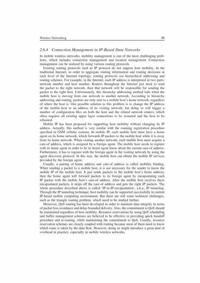
Wireless Networking 53
2.6.4 Connection Management in IP-Based Data Networks
In mobile wireless networks, mobility management is one of the most challenging prob-
lems, which includes connection management and location management. Connection
management can be realized by using various routing protocols.
Existing routing protocols such as IP protocol do not support host mobility. In the
traditional Internet, in order to aggregate routing information and routing decisions at
each level of the Internet topology, routing protocols use hierarchical addressing and
routing schemes. For example, in the Internet, each IP address is interpreted in two parts:
network number and host number. Routers throughout the Internet just need to send
the packet to the right network, then that network will be responsible for sending the
packet to the right host. Unfortunately, this hierarchy addressing method fails when the
mobile host is moving from one network to another network. According to hierarchy
addressing and routing, packets are only sent to a mobile host’s home network, regardless
of where the host is. One possible solution to this problem is to change the IP address
of the mobile host to an address of its visiting network, but doing so will trigger a
number of configuration files on both the host and the related network routers, which
often requires all existing upper layer connections to be restarted and the host to be
rebooted.
Mobile IP has been proposed for supporting host mobility without changing its IP
address. Actually, this method is very similar with the roaming registration procedure
specified in GSM cellular systems. In mobile IP, each mobile host must have a home
agent on its home network, which forwards IP packets to the mobile host while it is away
from its home network. When visiting another network, each mobile host must acquire a
care-of address, which is assigned by a foreign agent. The mobile host needs to register
with its home agent in order to let its home agent know about the current care-of address.
Furthermore, it has to register with the foreign agent in the visiting network by using the
agent discovery protocol. In this way, the mobile host can obtain the mobile IP services
provided by the foreign agent.
Usually, a pairing of home address and care-of address is called mobility binding.
When sending a packet to a mobile host, it is not necessary for the sender to know the
mobile IP of the mobile host. It just sends packets to the mobile host’s home address,
then the home agent will forward packets to its foreign agent by encapsulating each
IP packet with the mobile host’s care-of address. After the mobile host receives these
encapsulated packets, it strips off the care-of address and gets the right IP packets. The
whole procedure described above is called ‘IP-in-IP-encapsulation’, a.k.a., IP tunneling.
Through the IP tunneling technique, host mobility can be supported successfully in current
IP-based mobile computing environment. But there are still some technical challenges,
such as the triangle routing problem, which need to be studied further.
Moreover, QoS routing has been developed in order to maintain data integrity in terms
of packet loss avoidance and delay-bounded delivery. Also, the commitment to QoS should
be maintained regardless of host mobility. Resource reservations by using QoS scheduling
and buffer management schemes are believed to be effective in providing quick handoff
procedure and re-routing, while maintaining the commitment to QoS. Usually, resource
reservation schemes are closely coupled with routing because most of them need to know
which route is taken by the data flow. However, doing so might introduce a great deal of
overhead in practice, especially in mobile wireless networks.

54 Wireless Communications and Networking
(1) Location management: Location management is one of the key components of
mobility management, which deals with how to track a mobile host in mobile wireless
networks [56–59]. Host locations are derived by using two basic operations: location
update and location paging. Location update, also called registration, is the process by
which the network tracks the location of a mobile host not engaged in conversation.
A mobile host dynamically updates its location information, where a location area may
include one or more cells. Furthermore, when packets arrive, the network will send out a
polling signal to a location area for searching for the addressed mobile host. This process
is called paging.
Static location management would incur a great deal of overhead in terms of bandwidth
and power, since the paging area is fixed and equal to a local area, every time all of the
cells of a local area are paged. Moreover, whenever a mobile host moving into a new
location area, the location update procedure will be triggered, which is not efficient,
especially when a mobile host moves back and forth between two local areas.
Dynamic location management has been proposed in order to solve this problem. In
dynamic location management, the size of a local area keeps changing with the change of
user mobility and service. So far, there are three types of dynamic location management
strategies: time-based update, movement-based update and distance-based update [56].
Their performance varies under different movement patterns. Typically, there are two
movement patterns used in analyzing the performance of dynamic location management
strategies, one is i.i.d. (independent and identically distributed) movement, and the other
is Markovian movement. In the i.i.d. model, during a time slot, the probability that a user
is in cell i at the beginning of the slot is independent of the probability that it moves to
cell i + 1, moves to cell i − 1, or remains in cell i. On the other hand, in the Markovian
model, during a time slot, user movement during the current slot depends on its state
(stationary, right-move state, or left-move state) in the previous slots. Let X(t) be the
state during slot t , then X(t), t = 0, 1, 2 . . . is a Markov chain. The assumptions here are:
(1) time is slotted; (2) a user can move into at most one cell during each time slot; (3)
location update and paging are done at the beginning of each slot; and (4) paging can
be finished within one slot. In practice, these assumptions can be relaxed easily. Readers
may refer to [56] for more information about dynamic location management strategies
under the i.i.d. model.
2.6.5 QoS Handoff
4G wireless networks should support broadband data services to mobile users while still
retaining the commitment to QoS. Unlike its wired counterpart, where relatively there is
plenty of bandwidth and reliable channels are available, mobile wireless data networks
must face problems such as limited bandwidth, error-prone and time-varying channel and
mobility. In general, handoff happens at the cell border, where link quality is signifi-
cantly less reliable. Besides, link throughput is also crucial in order to lower the handoff
latency. Although link adaptation can improve wireless link throughput, handoff re-routing
schemes have to be chosen for achieving optimal routes during handoff.
Research on handoff re-routing for connection-oriented wireless networks has originated
from two different goals. The first goal is to ensure to establish an optimal route when
the mobile host moves to a new location. Although an optimal route can be selected

Summary 55
eventually, the handoff latency may be increased significantly owing to routing table
calculation and connection establishment. Another goal is to achieve the shortest handoff
latency by keeping the original route, and then extending this route hop-by-hop as the
mobile host is moving. However, in this way network resources will be wasted by many
redundant hops. So far, there have four types of connection-oriented handoff re-routing
schemes, which are anchored handoff re-route, multicast handoff re-route, chained handoff
re-route and classified handoff re-route.
In anchored handoff re-route [60], an anchor switch or router is designated for each
mobile host in the original connection route. During the lifetime of a connection, the
path that connects the anchor switches (anchor segments) will never change. Then, when
one of the mobile host moves to a new location, only part of the path which connects
the mobile host with its own anchor switch needs to be re-routed. This scheme avoids
establishing a whole new route for each handoff. However, anchor segments may cause
longer routes, looped routes, or higher complexity and packet losses.
In multicasting handoff re-route [61], incoming traffic for a mobile host is multicasted
to several surrounding base stations, which will buffer all packets for the mobile host
until it enters into a new location. This scheme can significantly reduce handoff latency.
But it expends much multicasting bandwidth for each user and requires excessive buffer
usage in those locations where the mobile host is not entering.
In chained handoff re-route [62], a temporary route is established by simply extending
the original route to the current location. This temporary route will be expired until an
optimal route is found. This scheme requires several intermediate routes that consume
bandwidth for each movement of the mobile host.
In classified handoff re-route [63], the source switch or router determines the new route
to the moving endpoints of an end-to-end connection, regardless of which endpoint has
moved. Thus, the number of intermediate routes is reduced by centralizing the establish-
ment of the new routes and preventing the need for establishing and terminating routes
while an endpoint is still moving. In this scheme, each endpoint switch or router will
divide the connections into two groups: delay sensitive and loss sensitive. Then, when
one (or both) of the endpoints of a connection moves, the endpoint switches will be able to
re-route the connection based on the traffic type by using different means of re-route. For
example, for delay sensitive connections, handoff latency is critical, so chained handoff
re-routing will be used; for loss sensitive connections, multicast re-routing can be adopted
in order to prevent data losses until an optimal route is calculated.
2.7 Summary
In this chapter, the fundamentals of wireless communications and networking have been
reviewed. We started with the characteristics and modeling of wireless channels, and
major slowing fading channels were introduced. We then focused on the popular link
adaptation techniques such as adaptive modulation and coding and HARQ as well as
cross-layer design of link adaptation, which have been widely adopted in wireless com-
munications. A comprehensive review has been provided. Since 4G wireless networks
are all IP networks, we discussed the basics of computer networks. Two network design
architectures, the OSI model and the TCP/IP model, were covered. Because multiplexing

56 Wireless Communications and Networking
is an important technique for enhancing wireless network capacity, the current major mul-
tiplexing methods were reviewed. In wireless networks using licensed frequency bands,
the concept of cellular networks has been widely adopted in order to improve frequency
utilization. As a result, mobility management and handoff are very important in order to
provide QoS to mobile users in cellular networks. The performance of major mobility
and location management schemes was also discussed.
References
1. B. S. Publishers, Wireless Communication . http://www.baltzer.nl/wicom/, 1999.
2. T. S. Rappaport, Wireless Communications: Principles and Practice. Prentice Hall, Inc., 1996.
3. W. Feller, An Introduction to probability Theory and Its Applications . John Wiley & Sons, Inc., 1968.
4. H. Stark and J. Woods, Probability, Random Processes and Estimation Theory for Engineers . Prentice
Hall, Inc., 1994.
5. J. G. Proakis, Digital Communications . New York: McGraw-Hill, 1995.
6. W. Jakes, Microwave Mobile Communications . John Wiley & Sons, Inc., 1974.
7. E. Gilbert, “Capacity of a Burst-Noise Channel,” The Bell System Technical Journal , Vol. 39, pp. 1253–63,
1963.
8. E. Elliott, “Estimates of Error Rates for Codes on Burst-Noise Channels,” The Bell System Technical
Journal , Vol. 42, pp. 1977–97, 1963.
9. S. Wilson, Digital Modulation and Coding . Prentice Hall, Inc., 1996.
10. F. swarts and H. Ferreira, “Markov Characterization of Digital Fading Mobile VHF Channels,” IEEE
Transactions on Vehicular Technology , Vol. 43, No. 4, pp. 977–85, 1994.
11. J. Garcia-Frias and P. Crespo, “Hidden Markov Models for Burst Error Characterization in Indoor Radio
Channels,” IEEE Transactions on Vehicular Technology , Vol. 46, No. 4, pp. 1106–20, 1997.
12. H. Wang and N. Moayeri, “Finite-Stae Markov Channel-A Useful Model for Radio Communication
Channels,” IEEE Transactions on Vehicular Technology , Vol. 44, No. 1, pp. 163–71, 1995.
13. H. Wang and P. Chang, “On Verifying the First-Order Markovian Assumption for a Rayleigh Fading
Channel Model,” IEEE Transactions on Vehicular Technology , Vol. 44, No. 2, pp. 353–57, 1996.
14. B. Vucetic, “An Adaptive Coding Scheme for Time-Varying Channels,” IEEE Transactions , Vol. 30,
No. 5, pp. 653–63, 1991.
15. M.-S. Alouini, X. Tang, and A. Goldsmith, “An Adaptive Modulation Scheme for Simultaneous Voice
and Data Transmission over Fading Channels,” IEEE Journal on Selected Areas in Communications , Vol.
17, No. 5, pp. 837–50, 1999.
16. J. Cavers, “Variable-Rate Transmission for Rayleigh Fading Channels,” IEEE Transactions on Communi-
cations , Vol. COM-20, No. 1, pp. 15–22, 1972.
17. W. Webb and R. Steele, “Variable Rate QAM for Mobile Radio,” IEEE Transactions on Communications ,
Vol. 43, No. 7, pp. 2223–30, 1995.
18. J. Bingham, “Multicarrier Modulation for Data Transmission: An Idea Whose Time Has Come,” IEEE
Communications Magzine, Vol. 28, No. 5, pp. 5–14, 1990.
19. T. Keller and L. Hanzo, “Adaptive multicarrier modulation: a convenient framework for time-frequency
processing in wireless communications,” Proceedings of the IEEE , Vol. 88, No. 5, pp. 611–40, 2000.
20. S. Alamouti and S. Kallel, “Adaptive Trellis-Coded Multiple-Phase-Shift Keying for Rayleigh Fading
Channels,” IEEE Transactions on Communications , Vol. 42, No. 6, pp. 2305–14, 1994.
21. A. Goldsmith and S. Chua, “Variable-Rate Variable-Power MQAM for Fading Channels,” IEEE Transac-
tions on Communications , Vol. 45, No. 10, pp. 1218–30, 1997.
22. X. Qiu and K. Chawla, “On the Performance of Adaptive Modulation in Cellular Systems,” IEEE Trans-
actions on Communications , Vol. 47, No. 6, pp. 884–95, 1999.
23. K. Balachandran, S. Kadaba, and S. Nanda, “Channel quality estimation and rate adaptation for cellular
mobile radio,” IEEE Journal on Selected Areas in Communications , Vol. 17, No. 7, pp. 1244–56, 1999.
24. A. Goldsmith and C. S. G., “Adaptive Coded Modulation for Fading Channels,” IEEE Transactions on
Communications , Vol. 46, No. 5, pp. 595–602, 1998.

References 57
25. D. Goeckel, “Adaptive Coding for Time-Varying Channels Using Outdated Fading Estimates,” IEEE
Transactions on Communications , Vol. 47, No. 6, pp. 844–55, 1999.
26. F. Babich, “Considerations on adaptive techniques for time-division multiplexing radio systems,” IEEE
Transactions on Vehicular Technology , Vol. 48, No. 6, pp. 1862–73, 1999.
27. C. Wong and L. Hanzo, “Upper-bound performance of a wide-band adaptive modem,” IEEE Transactions
on Communications , Vol. 48, No. 3, pp. 367–9, 2000.
28. C. C. et al., “Adaptive Radio for Multimedia Wireless Links,” IEEE Journal on Selected Areas in Com-
munications , Vol. 17, No. 5, pp. 793–813, 1999.
29. V. Lau and S. Maric, “Variable rate adaptive modulation for DS-CDMA,” IEEE Transactions on Commu-
nications , Vol. 47, No. 4, pp. 577–89, 1999.
30. M. Pursley and J. Shea, “Adaptive nonuniform phase-shift-key modulation for multimedia traffic in wire-
less networks,” IEEE Journal on Selected Areas in Communications , Vol. 18, No. 8, pp. 1394–407,
2000.
31. J. Torrance and L. Hanzo, “Latency and networking aspects of adaptive modems over slow indoors rayleigh
fading channels,” IEEE Transactions on Vehicular Technology , Vol. 48, No. 4, pp. 1237–51, 1999.
32. J. Torrance, L. Hanzo, and T. Keller, “Interference aspects of adaptive modems over slow rayleigh fading
channels,” IEEE Transactions on Vehicular Technology , Vol. 48, No. 5, pp. 1527–45, 1999.
33. L. Chang, “Throughput Estimation of ARQ Protocols for a Rayleigh Fading Channel Using Fade- and
Interfade-Duration Statistics,” IEEE Transactions on Vehicular Technology , Vol. 40, No. 1, pp. 223–29,
1991.
34. A. Goldsmith, Wireless Communications. Cambridge University Press, 2005.
35. G. J. Foschini, “Layered space-time architecture for wireless communication in fading environments when
using multi-element antennas,” Bell System Tech. J., pp. 41–59, 1996.
36. P. Wolniansky, G. Foschini, G. Golden, and R. Valenzuela, “V-blast: an architecture for realizing very
high data rates over the rich-scattering wireless channel,” in Proc. URSI Intl. Symp. Sign. Syst. Electr.,
Oct. 1998, pp. 295–300.
37. S. Alamouti, “A simple transmit diversity technique for wireless communications,” IEEE J. Sel. Areas
Commun., pp. 1451–1458, Oct. 1998.
38. A. Paulraj, R. Nabar, and D. Gore, Introduction to Space-Time Wireless Communications . Cambridge
University Press, 2003.
39. L. Zheng and D. N. Tse, “Communication on the grassmann manifold: A geometric approach to the
noncoherent multi-antenna channel,” IEEE Trans. Inf. Theory , Vol. 48, pp. 359–383, Feb. 2002.
40. E. Biglieri, R. Calderbank, A. Constantinides, A. Goldsmith, A. Paulraj, and H. V. Poor, MIMO Wireless
Communications . Cambridge University Press, 2007.
41. V. Tarokh, N. Seshadri, and A. Calderbank, “Space-time codes for high data rate wireless communications:
performance criterion and code construction,” IEEE Trans. Inf. Theory , Vol. 44, No. 2, pp. 744–765, Mar.
1998.
42. V. Tarokh, H. Jafarkhani, and A. Calderbank, “Space-time block codes from orthogonal designs,” IEEE
Trans. Inf. Theory , Vol. 45, pp. 1456–1467, Jul. 1999.
43. (2004) 3GPP TR 25.848 V4.0.0, Physical Layer Aspects of UTRA High Speed Downlink Packet Access
(release 4).
44. (1999) 3GPP2C.S0002-0 Version 1.0, Physical Layer Standard for cdma2000 Spread Spectrum Systems.
45. A. Doufexi, S. Armour, M. Butler, A. Nix, D. Bull, J. McGeehan, and P. Karlsson, “A Comparison of
the HIPERLAN/2 and IEEE 802.11a Wireless LAN Standards,” IEEE Communication Magazine, Vol. 40,
pp. 172–180, May 2002.
46. (2002) IEEE Standard 802.16 Working Group, IEEE Standard for Local and Metropolitan Area Networks
Part 16: Air Interface for Fixed Broadband Wireless Access Systems.
47. S. Lin and D. Costello, Error Control Coding: Fundamentals and Applications . Englewood Cliffs, NJ:
Prentice-Hall, 1983.
48. S. Lin, D. Costello, and M. Miller, “Automatic-repeat-request Error-control Schemes,” IEEE Communi-
cation Magazine, Vol. 22, pp. 5–17, Dec. 1984.
49. J. hagenauer, “Rate-compatible punctured convolutional codes (rcpc codes) and their applications,” IEEE
Trans. Commun., Vol. 36, pp. 389–400, Apr. 1988.

58 Wireless Communications and Networking
50. Q. Zhang and S. A. Kassam, “Hybrid arq with selective combining for fading channels,” IEEE J. Sel.
Areas Commun., Vol. 17, pp. 867–880, May 1999.
51. M. B. Pursley and D. J. Taipale, “Error probabilities for spread-spectrum packet radio with convolutional
codes and viterbi decoding,” IEEE Trans. Commun., Vol. COM-35, pp. 1–12, Jan. 1987.
52. Q. Liu, S. Zhou, and G. B. Giannakis, “Cross-layer combining of adaptive modulation and coding with
truncated arq over wireless links,” IEEE Transactions on Wireless Communications , Vol. 3, pp. 1746–1755,
Sep. 2004.
53. M. Alouini and A. J. Goldsmith, “Adaptive modulation over nakagami fading channels,” Kluwer J. Wireless
Communications , Vol. 13, pp. 119–143, May 2000.
54. A. J. Viterbi, “Convolutional codes and their performance in communication systems,” IEEE Trans. Com-
mun., Vol. COM-19, pp. 751–772, Oct. 1971.
55. A. S. Tanenbaum, Computer Networks. Upper Saddle River, NJ: Prentice Hall, 2003.
56. Bar-Noy, A., Kessler, I., and Sidi, M., “Mobile Users: To Update or not to Update?” Proceeding of IEEE
INFOCOM’94 , Vol. 2, 1994.
57. Liu, T. et al., “Mobility Modeling, Location Tracking, and Trajectory Prediction in Wireless ATM Net-
work,” IEEE JSAC , Vol. 6, No. 6, 1998.
58. Rose, C. and Yates, R., “Location Uncertainty in Mobile Networks: a theretical framework,” Technical
Report , 1996.
59. SAC 2001, “Analysis of Dynamic Location Management for PCS Networks,” ACM SAC2001 , 2000.
60. Veeraraghavan, M. et al., “Mobility and Connection Management in a Wireless ATM LAN,” IEEE JSAC ,
Vol. 15, No. 1, 1997.
61. Ghai, R. and Singh, S., “An Architecture and Communication Protocol for Picocellular Networks,” IEEE
Personal Communications Magazine, Vol. 1, 1994.
62. Rajagopalan, B, “Mobility Management in Integrated Wireless-ATM Networks,” ACM-Baltzer Journal of
Mobile Networks and Applications (MONET), Vol. 1, No. 3, 1996.
63. McNair, J. et al., “Handoff Rerouting Scheme for Multimedia Connections in ATM-based Mobile Net-
works,” Proceeding of IEEE Fall VTC’00 , 2000.

3
Video Codingand Communications
3.1 Digital Video Compression – Why and How Much?
Uncompressed standard definition (SD) video, captured by following the ITU-R 601 4:2:2
standard [1] with 10 bits per pixel, consists of a 270 Mbits/sec bit rate. The typical chan-
nel capacity that is available and is used for the transmission of a TV channel is less than
6 Mbits/sec and averages around 3 Mbits/sec. There is a strong push to further reduce
that capacity due to economic reasons. This implies that one is required to remove more
than 98% of the original information and compress the digital video to less than 2%
of the initial bit rate. It requires more than 50 × compression factor. It is not possible to
achieve that amount of compression without loss of information. The loss of information
adds distortion to the decoded video which appears as a degradation of visual quality in
the displayed video. Therefore, one of the key goals of a compression algorithm is, at
a given bit rate, to add as little distortion in the decoded video as possible and to lose
the information so that the degradation is as invisible as possible. To minimize the per-
ceptual distortion some processing steps are taken before encoding the video. The typical
pre-compression steps taken for consumer applications are to compress only the visible
part of the video, reduce the number of bits per pixel from 10 to 8 bits and reduce the color
resolution before compressing the video.
The visible part of a frame of video contains between 704 and 720 pixels horizon-
tally and 483 lines vertically in the 525-line system used in North America (the other
commonly used system outside North America is the 625-line system with 704 to 720
pixels horizontally and 576 active lines vertically). Owing to the inherent block processing
nature of the most commonly used compression schemes, the number of pixels used to
represent the visible part of the video needs to be a multiple of 16 and is either 704 or 720.
Vertically, the number of lines is required to be a multiple of 16 for progressively scanned
video and a multiple of 32 for interlaced scanned video. Therefore, 480 lines are com-
monly used to represent the visible portion of an SD video in the 525-line system. Thus
a video picture at SD consists of maximum of 720 × 480 = 345 600 pixels. Assigning
4G Wireless Video Communications Haohong Wang, Lisimachos P. Kondi, Ajay Luthra and Song Ci
© 2009 John Wiley & Sons, Ltd. ISBN: 978-0-470-77307-9

60 Video Coding and Communications
8 bits for the luminance of each of the pixels provides 720 × 480 × 8 = 2 764 800
bits for the luminance part of a frame of a SD video. In the ITU-R 601 4:2:2 standard
the color resolution is reduced horizontally by a factor of 2. The color information is
represented by two difference signals (R-Y, B-Y) and is assigned to only every other
pixel horizontally. Therefore, an SD video frame contains 360 × 480 × 8 × 2 = 2 764
800 bits for the chrominance part. Counting both luminance and chrominance parts, it
requires 2 × 2 764 800 = 5 529 600 bits to represent a SD video frame. In North America,
standard definition video is sent at a rate of 30 (or 29.97) frames per sec (the 625-line
system uses a rate of 25 frames/sec). Therefore, the bandwidth required for the visible part
of the video following the above mentioned format is 5 529 600 × 30 bits/sec which is
approximately 165 Mbits/sec. For consumer applications, one more compromise is made
in the representation of a video frame – color information is decimated by a factor of 2
vertically, i.e. color information is kept only for every other pixel (line) vertically. This is
also known as 4:2:0 chroma format. In this format, uncompressed SD video requires 1.5
× 2 764 800 × 30 which is about 124 Mbits/sec. This is a very large number in compar-
ison to the bandwidth available for the transmission of digital television. Similarly, the
storing of uncompressed video also requires an uneconomically large storage capacity.
As an example, a 2 hour long movie at a rate of 124 Mbit/sec requires more than 110
GBytes of storage capacity. It is much larger than what is available and practical today.
Hence there has been a strong desire to improve video coding efficiency.
In High Definition TV (HDTV), two video formats are commonly used in North
America – 1920 × 1080 size frames at 30 frames/sec and 1280 × 720 size frames at
60 frames/sec. In uncompressed 4:2:0 formats, they require about 750 Mbits/sec and 660
Mbits/sec respectively. It will require about 675 GBytes to store one 2+ hrs movie.
Recently, many users have expressed an interest in using 1920 × 1080 size frames at a
rate of 60 frames/sec. In the uncompressed 4:2:0 format, this requires around 1.5 Gbits/sec
of bandwidth or a storage capacity of more than 1.2 Terra Bytes for a 2+ hrs long movie!
In addition, with the availability of high quality large TV displays 10 bits and/or 4:4:4
format and/or higher than 1920 × 1080 resolution of video may also be used in digital TV
in the future. Thus, the introduction of HDTV, and the resolution higher than what is used
in HDTV today, puts further pressure on channel and storage capacity and emphasizes
the need for having a compression algorithm with very high coding efficiency.
3.2 Basics
Now that we have described the need for video compression, we will discuss the basics
of video representation, including scanning and color representation.
3.2.1 Video Formats
3.2.1.1 Scanning
Video pictures consist of a certain number of scanned lines. Each line is scanned from left
to right and various standards specify different numbers of scanned lines in the vertical
dimension. In the 525 line standard for SDTV, commonly used in North America, there
are total of 525 lines of which the active visual area consists of 483 lines. Another
commonly used standard consists of a total of 625 lines out of which the active visual

Basics 61
area consists of 576 lines. When these standards were developed, it was very expensive
to develop the devices with that many lines at the specified frame rates – 30 (or 29.97)
frames/sec for 525 line systems and 25 frames/sec for 625 line systems. Therefore, in
order to reduce the bandwidth required to capture and display a frame, it was scanned in
an interlaced format where a frame consists of two fields. In an interlaced format, each
field consists of half the number of lines – one with odd numbered lines (line numbers 1,
3, 5 and so on) and another with even numbered lines (line numbers 2, 4, 6 and so on),
as shown in Figure 3.1. In this figure the solid lines correspond to field 1 and the dotted
lines correspond to field 2.
Field 1 is also called the top field and field 2 the bottom field. It should also be noted
that the top field (field 1) is not always displayed first. The syntaxes of the compression
standards allow one to specify which field needs to be displayed first.
In HDTV there are two most commonly used formats: one with 1080 lines and other
one with 720 lines in the visual area of a frame. In the 1080 line format frames are
captured at 24 frames/sec or 30 frames/sec. The 24 frames/sec rate is used for movie
material. In the 30 frames/sec format, each frame is scanned in the interlaced format
consisting of two fields (top and bottom) at a rate of 60 fields/sec. In the 720 line format
the frames are captured with progressive scanning at 60 frames/sec rate. The 1080 line
format consists of 1920 pixels horizontally in each line and the 720 line format consists of
1280 pixels horizontally. These numbers are such that the picture aspect ratio (1920:1080
and 1280:720) is 16:9 and the pixel rate is approximately similar – 62 208 000 pixels/sec
(1920 × 1080 × 30) and 55 296 000 pixels/sec (1280 × 720 × 60).
There has been a heated discussion in the technical community as to which scanning
format – interlaced or progressive – is better. They both have their plusses and minuses.
Without going into that argument, the AVC/H.264 standard provides tools for both, inter-
laced and progressive, formats. However, with the advancement in display and video
capturing technology, the progressive format is expected to dominate and the interlaced
format is expected to fade away in the future.
3.2.1.2 Color
Color TV displays and many video capture devices are based on representing pixels in
a video frame in terms of three primary colors Red (R), Green (G) and Blue (B) [2, 3].
However, before video compression, RGB values are transformed into Y, Cr, Cb where
Field 1
Field 2
Figure 3.1 Interlaced scanned frame

62 Video Coding and Communications
Y, also known as luminance or luma, corresponds to luminance values, Cr and Cb, also
known as chrominance or chroma, correspond to the two color difference signals R-Y and
B-Y. When there are chroma values present for each pixel, it is called 4:4:4 sampling.
The roots of this nomenclature lie in the analog video domain. When analog composite
video was sampled, it was sampled at four times the frequency of the color sub-carrier
(4 × fsc). There were two dominant standards for analog video: NTSC (National Television
System Committee) and PAL (Phase Alternating Line). The sub-carriers for the NTSC and
PAL systems were at different frequencies. Therefore, as a compromise, ITU-R (known
as CCIR before changing its name to ITU-R) developed a universal international standard
to sample the luminance part of analog video at 13.5 Msamples/sec rate [1]. The Human
Visual System is relatively less sensitive to chroma resolution than to luma resolution.
Therefore, many applications do not use the same chroma resolution as luma resolution.
In some systems it was sampled at 1/4th the rate of Luma sampling rate. To signify that
luma and chroma are sampled at different rate, the format with the chroma sampling
rate of 3.375 Msamples/sec was called 4:1:1 (luma is sampled at four times the rate of
chroma). In the ITU-R 601 4:2:2 format, chroma is sampled at half the rate of luma. The
nomenclature 4:2:2 signified that chroma was sampled at half the rate (13.5/2 = 6.75
Msamples/sec). In the early days the number 4 was closely tied to the 13.5 Msamples/sec
rate. So, in the systems where the luma was sampled at twice the rate, it was denoted as
8:4:4 or 8:8:8 depending upon the relative sampling rates of luma and chroma. However,
as High Definition Tele Vision (HDTV) became real the same nomenclature 4:4:4 and
4:2:2 was used even though the sampling rate of each luma and chroma component is
much higher than for SDTV. So, currently 4:2:2 merely signifies that chroma sampling
rate is half of the luma sampling rate.
In the early digital video applications, chroma was sub-sampled only horizontally. Ver-
tically it had the same number of samples in a picture as luma samples. However, in
digital video compression applications, in addition to horizontal decimation, the chromi-
nance is also decimated vertically by a factor of 2 before encoding. This format is called
4:2:0 where last digit 0 does not have any real significance. Conversion from 4:4:4 to
4:2:0 is done as a pre-processing step to the digital video encoding. As this step also
reduces the number of bits representing digital video, it can also be seen as the first step
of digital video compression.
Figure 3.2(a) illustrates the 4:4:4 sampling structure. Here X marks represent the loca-
tions of luma samples and circles represent the locations of chroma samples. Figure 3.2(b)
shows the 4:2:2 sampling structure. In this format, chroma samples are present with every
other luma sample horizontally. Figure 3.2(c) depicts the 4:2:0 sampling structure used
in MPEG-2 [4] and AVC/H.264 [5] and Figure 3.2(d) shows the 4:2:0 sampling structure
used in MPEG-1 [6]. In MPEG-1 the chroma sample is centered horizontally as well
as vertically between the luma samples. Note that, as shown in Figure 3.3, for inter-
laced video, only one out of four frame-lines in a field has chroma information in 4:2:0
sampling format. This causes color smearing. It is generally not objectionable in consumer
applications but becomes objectionable in studio and video production applications. For
this reason, 4:2:2 is more popular in a studio and video production environment. In pro-
gressively scanned video 4:2:0 sampling does not introduce significant color spreading and
provides symmetrical horizontal and vertical chroma resolution. However, 4:2:2 remains
a very popular digital video capturing and storing standard for a progressively scanned

Basics 63
O OO O
…
X X X X…
X X X X…O OO OX X X X…O OO O
X X X X…O OO OX X X X…O OO O
XOXOXO
XOXO
Figure 3.2(a) 4:4:4
sampling
X X X X…
…
X X X X…O O
X X X X…O O
X X X X…O O
XOX
XO
XOX X X X… X
O O
O O O
O
Figure 3.2(b) 4:2:2
sampling
…
X X X X… X
X X X X…O O OX
X X X X… X
X X X X…O O OX
Figure 3.2(c) 4:2:0
sampling in MPEG-2
and AVC
…
X X X X… X
X X X X…O O OX
X X X X… X
X X X X…O O OX
Figure 3.2(d) 4:2:0
sampling in MPEG-1
video also. Therefore, conversion to 4:2:0 is required before encoding the video. This
introduces some artifacts, especially if it is done on multiple occasions.
The AVC/H.264 standard is defined for all three 4:4:4, 4:2:2 and 4:2:0 color formats. As
4:2:2 is a very popular video capturing format, a natural question arises – should one apply
the digital video encoding algorithm directly in the 4:2:2 domain as opposed to first going
down to the 4:2:0 domain. Both digital video encoding and chroma sub sampling introduce
artifacts but they look visually different. Therefore, the answer depends on the type of
sequences, the bit rates, the compression standard and the pre-processing technology used
to do the conversion. With current pre-processing and video coding technology typically
used in the products, generally, at higher bit rates (for example, above 12 Mbits/sec for
MPEG-2) one obtains better video quality by staying in the 4:2:2 domain and at lower
bit rates (such as below 6 Mbits/sec for MPEG-2) one obtains less objectionable artifacts
by first going from 4:2:2 to 4:2:0 before encoding.
(a) Top field (b) Bottom field
…
X X X X… XO O O
X X X X… XO O O
X X X X… X
…
X X X X… X
X X X X…O O O X
X X X X… X
Figure 3.3 Chroma locations in 4:2:0 format for Interlace scanned video

64 Video Coding and Communications
3.2.1.3 Luminance, Luma, Chrominance, Chroma
The Cathode Ray Tube (CRT) of television does not have linear electrical to optical
transfer characteristics. Generally, the optical output is proportional to the input voltage
raised to some power. That power is represented by the Greek character gamma (γ ) [7].
The value of γ depends on the display type. For CRTs it is around 2.2. Therefore, in
order to compensate for that non-linear behavior, cameras go through a gamma correction
process where in the optical to electrical conversion step the inverse of gamma is used. To
distinguish between the pre-gamma corrected (linear) stage and the post gamma corrected
stage, the brightness and color difference signals before correction are called luminance
and chrominance signals respectively and after the gamma correction those signals are
called luma and chroma signals respectively. As all the video compression and processing
in an encoder and decoder happens in the gamma corrected domain, the recognition of
that difference is acknowledged in the AVC/H.264 video coding standard (see Chapter 5)
and the terms Luma and Chroma are used.
3.3 Information Theory
So far we have discussed the basics of video representation. Before continuing with video
compression, we will review some of the basic aspects of information theory. Informa-
tion theory is the fundamental mathematical theory that governs compression and sets
its theoretical limits. More information can be found in [8–10]. Let F = {Fn} repre-
sent an information source consisting of a number of samples. Each sample Fn of the
source is a random variable. In this discussion, we are considering discrete sources .
Thus, Fn is a discrete random variable and can only take values from a discrete set
(alphabet) of symbols A = {a1, a2, . . . , aL}. In the context of video coding, a discrete
source may be, for example, the output of a quantizer. A discrete source can alterna-
tively be seen as a discrete-state random process [11]. In this chapter, we only consider
stationary sources (processes). A source is stationary if the distribution of Fn does
not depend on the index n, and the joint distribution of a group of N samples is
invariant with respect to a common shift in the index. Let pFn(f ) be the probabil-
ity mass function (pmf) of discrete random variable (sample of the source) Fn. Also, let
pFn+1,Fn+2,...,Fn+N(f1, f2, . . . , fN ) be the joint pmf of N consecutive samples of the source
F. Furthermore, let pFn|Fn−1,Fn−2,...,Fn−M(fM+1|fM , fM−1, . . . , f1) be the conditional pmf
of sample FM given the previous M samples. For simplicity, we will use interchange-
ably the notations p(f ), p(f1, f2, . . . , fN ) and p(fM+1|fM , fM−1, . . . , f1) to denote the
preceding functions when there is no risk of confusion.
A stationary source is called independent identically distributed (i.i.d.) if:
p(f1, f2, . . . , fN ) = p(f1)p(f2) · · · p(fN ) (3.1)
or equivalently,
p(fM+1|fM , fM−1, . . . , f1) = p(fM+1) (3.2)

Information Theory 65
3.3.1 Entropy and Mutual Information
The entropy of a discrete random variable F with alphabet A is defined as
H(F) = −∑
f ∈A
pF (f ) log2 pF (f ) (3.3)
Since a base-2 logarithm is used in the above definition, the unit for entropy is bits/
sample.
Entropy is a measure of the uncertainty about a random variable F . Let us consider
the example of a random variable F that corresponds to a coin toss and takes on values
A = {heads, tails}. Let p be the probability of ‘heads’. Then, 1 − p is the probability of
‘tails’. The entropy of such a random variable is:
H(F) = −p log2 p − (1 − p) log2(1 − p) (3.4)
Let us assume that the coin is not fair and the outcome is always ‘heads’. Then, p = 1.
Thus, H(F) = −1 log2 1 − 0 log2 0. Assuming that 0 log2 0 = limq→0
q log2 q = 0, it is clear
that H(F) = 0. Similarly, if the outcome is always ‘tails’, we also have H(F) = 0. The
entropy of this random variable is maximum when the coin is fair and p = 0.5. In that
case, H(F) = 1bit/sample. If the coin is unfair and always gives the same result, then,
there is no uncertainty in the random variable F . The outcome of the experiment is
totally expected. We gain no information when we are told the outcome of such an
experiment. On the other hand, when p = 0.5, there is maximum uncertainty in the
random variable F . Neither ‘heads’ nor ‘tails’ is favored against the other outcome. The
greater the uncertainty, the greater the amount of information we acquire when we learn
the outcome of the experiment. Thus, the uncertainty about a random variable can be
considered as the information that is conveyed by it.
The joint entropy of two discrete random variables F and G with a joint pmf pF,G(f, g)
and alphabets Af and Ag, respectively is defined as:
H(F, G) = −∑
f ∈Af
∑
g∈Ag
pF,G(f, g) log2 pF,G(f, g) (3.5)
The conditional entropy of discrete random variable F given discrete random variable G
is defined as:
H(F |G) = −∑
g∈Ag
pG(g)∑
f ∈Af
pF |G(f, g) log2 pF |G(f, g) (3.6)
where pF |G(f, g) is the conditional pmf of F given G and pG(g) is the marginal pmf
of G.
We are now ready to extend the entropy definitions from random variables to informa-
tion sources.

66 Video Coding and Communications
The Nth order entropy of a discrete stationary source F is the joint entropy of N
consecutive samples F1, F2, . . . , FN of F:
HN (F) = H(F1, F2, . . . FN ) = −∑
[f1,f2,...,fN ]∈AN
p(f1, f2, . . . , fN ) log2 p(f1, f2, . . . , fN )
(3.7)
where p(f1, f2, . . . , fN ) is the joint pmf of N consecutive samples of F and AN is the
N -fold Cartesian product of A.
The Mth order conditional entropy of a discrete stationary source F is the conditional
entropy of a sample FM+1 given its previous M samples FM , FM−1, . . . , F1:
HC,M(F) = H(FM+1|FM , FM−1, . . . , F1)
=∑
[f1,f2,...,fN ]∈AN
p(f1, f2, . . . , fM)H(FM+1|fM , FM−1, . . . , f1) (3.8)
where
H(FM+1|fM , FM−1, . . . , f1) = −∑
fM+1∈A
p(fM+1|fM , fM−1, . . . , f1)
× log2 p(fM+1|fM , fM−1, . . . , f1)
and p(fM+1|fM , fM−1, . . . , f1) is the Mth order conditional pmf of F.
We will also define the entropy rate of a discrete source as:
H(F) = limN→∞
1
NHN (F) (3.9)
It can be shown that the entropy rate is also equal to
H(F) = limN→∞
HC,N (F) (3.10)
3.3.2 Encoding of an Information Source
Let us assume that we wish to encode a particular realization {fn} of a discrete source F
with alphabet A = {a1, a2, . . . , aL}. We will be assigning a binary code word cn to each
sample of the realization fn. We will refer to this procedure as scalar lossless coding . We
will need to design a one-to-one mapping between each element of the source alphabet
an and a binary code word cn. The coding is called lossless because the mapping is such
that the original sequence of source symbols can always be recovered without loss from
the stream of binary code words. In order for this to happen, the coded sequence must be
uniquely decodable. This means that the stream of binary code words must correspond to
only one possible sequence of source symbols. Let l(ai) be the length (in bits) of the code

Information Theory 67
word that corresponds to symbol ai . Then, the average code word length for encoding a
source realization {fn} is:
R =∑
ai∈A
p(ai)l(ai) (3.11)
We will also refer to R as the bit rate. Its unit is bits per sample.
The following theorem can be proven:
Theorem 3.1
The minimum bit rate R required to represent a discrete stationary source F using scalar
lossless coding (that is, by assigning one code word to each sample) satisfies:
H1(F) ≤ R ≤ H1(F) + 1 (3.12)
The lower bound of the above inequality cannot always be achieved. It is achievable
when the symbol probabilities are negative powers of 2. That is, p(ai) = 2−mi for a set
of integers {m1, m2, . . . , mL}. How far the minimum bit rate is from the lower bound
depends on the actual symbol probabilities.
It becomes clear that the optimal scalar lossless encoding for a particular discrete
stationary source can have a bit rate that is up to one bit per sample greater than the
entropy. It is possible to encode the source so that the average number of bits per sample is
arbitrarily close to H1(F).This can be accomplished by assigning a binary code word to a
large number N of consecutive source symbols. Thus, we can treat N source samples as
a vector sample that comes from vector source with alphabet AN. The first order entropy
of the vector source is the Nth order entropy of the original source:
HN (F) ≤ RN ≤ HN (F) + 1 (3.13)
where RN
is the minimum bit rate of the vector source.
It can be proven for an i.i.d. source that HN (F) = N · H1(F). It is clear that by encoding
one sample of the vector source, we are encoding N samples of the original source. Then,
RN = RN
Nwill be the average number of bits per original sample that results from the
vector sample encoding. Then,
N · H1(F) ≤ N · RN ≤ N · H1(F) + 1 (3.14)
and
H1(F) ≤ RN ≤ H1(F) +1
N(3.15)
Thus, for an i.i.d. source, the average code word length can be made arbitrarily close to
the first order entropy of the source by encoding a large number N together. If the source
is not necessarily i.i.d., we have:
HN (F)
N≤ RN ≤
HN (F)
N+
1
N(3.16)

68 Video Coding and Communications
Then, as N → ∞ we have
limN→∞
RN = limN→∞
HN (F)
N= H(F) (3.17)
Thus, we can say that the bit rate can always be made arbitrarily close to the source
entropy rate by encoding a large number of original source samples together.
Instead of using vector coding, we can improve coding efficiency by using conditional
coding , also known as context-based coding . In Mth order conditional coding, the code
word for the current sample is selected taking into account the pattern formed by the
previous M samples. We will refer to such as pattern as the context . We design a separate
code book for each of the possible contexts based on the conditional distribution of the
output sample given the context. If the size of the source alphabet is L, then, the maximum
number of contexts for Mth order conditional coding is LM . Applying the theorem to the
conditional distribution under context m, we get:
HmC,M(F) ≤ R
m
C,M ≤ HmC,M(F) + 1 (3.18)
where HmC,M(F) is the entropy of the Mth order conditional distribution under context m
and Rm
C,M is the minimum bit rate that can be achieved when encoding under context m.
If pm represents the probability of context m, the average minimum bit rate using Mth
order conditional coding is:
RC,M =∑
m
pmRm
C,M (3.19)
Then, it can be shown that:
HC,M(F) ≤ RC,M ≤ HC,M(F) + 1 (3.20)
When M → ∞, we get:
H(F) ≤ limM→∞
RC,M ≤ H(F) + 1 (3.21)
Conditional coding can achieve a better coding efficiency than scalar coding because
H(F) < H1(F), except when the source is i.i.d., in which case H(F) = H1(F). However,
whether Mth order conditional coding is more efficient than Nth order vector coding
depends on the actual source statistics.
3.3.3 Variable Length Coding
So far, we have discussed theoretical lower bounds on the bit rate with which an infor-
mation source can be coded. However, the previously presented theory does not give us
a means for encoding the information source in order to achieve these bounds. Binary
encoding corresponds to assigning a binary code word to each symbol of an information
source. As mentioned previously, we are interested in lossless coding, where there exists
a one-to-one mapping between each symbol and a binary code word and the original

Information Theory 69
sequence of source symbols can always be recovered from the binary bit stream. We will
also refer to lossless codes as uniquely decodable codes. An important subset of lossless
codes is the prefix codes . A code is a prefix code if no code word is a prefix of another
valid code word in the code. This means that the beginning bits of a code word do not
correspond to another code word. Clearly, prefix codes are always uniquely decodable.
Another property of prefix codes is that they are instantaneously decodable. This means
that we can decode a group of bits into a symbol if it matches a valid code word and we
do not have to wait for more bits to arrive, as may be the case for lossless but non-prefix
codes. Imposing a code to be a prefix code is a stronger requirement than just being a
lossless code. However, it can be proven that no non-prefix uniquely decodable codes can
outperform prefix codes in terms of bit rate. Thus, prefix codes are used in all practical
applications.
A code is fixed-length if every code word has the same number of bits. If the size of
the source alphabet is L, then the number of bits that need to be assigned for each code
word is⌊
log2 L⌋
. As we discussed earlier, the lower bound for the bit rate is equal to
the source entropy rate H(F) (or the first order entropy H1(F) for i.i.d. sources). Since
the bit rate (average code word length) is weighted by the probability of each symbol, it
is inefficient in most cases to assign the same number of symbols to low-probability and
high-probability symbols. It can be shown that fixed-length coding is optimal only in the
case when all symbol probabilities are equal. The lower bounds will be achieved if all
symbol probabilities are equal and negative powers of 2.
Intuitively, to minimize the average code word length, we will need to assign
shorter codes to high-probability symbols and longer codes to low-probability symbols.
Variable-Length Coding (VLC) assigns code words of different lengths to each symbol.
We next describe two popular VLC methods: Huffman coding and arithmetic coding .
Huffman Coding
Let us assume that we wish to encode a discrete stationary source with alphabet
A = {a1, a2, . . . , aL} and pmf p(al). Huffman coding is a VLC method that assigns
shorter code words to higher probability symbols. Huffman coding assigns prefix codes.
It can be shown that, when Huffman coding is applied to individual symbols (scalar
lossless coding), the resulting bit rate R is the minimum possible bit rate R that can be
achieved and satisfies the theorem H1(F) ≤ R ≤ H1(F) + 1. Thus, Huffman coding is
optimal for scalar lossless coding in terms of bit rate.
The Huffman coding algorithm is as follows:
1. Arrange the symbols in terms of decreasing probability order and consider them as
leaf nodes of a tree.
2. While more than one nodes remain:
a. Arbitrarily assign ‘1’ and ‘0’ to the two nodes with the smallest probabilities.
b. Merge the two nodes with the smallest probabilities to form a new node with a
probability that is the sum of the probabilities of the two nodes. Go back to step 1.
3. Determine the code word for each symbol by tracing the assigned bits from the cor-
responding leaf node to the top of the tree. The first bit of the code word is at the top
of the tree and the last bit is at the leaf node.

70 Video Coding and Communications
0.70
Symbol Probability
“a”
“b”
“c”
“d”
0.17
0.10
0.03 0
1 0
0.13
0.30
1.00
1 0
1
Figure 3.4 A Huffman coding example
Figure 3.4 shows an example of the Huffman coding of a source that emits symbols
‘a’, ‘b’, ‘c’ and ‘d’ with probabilities 0.70, 0.17, 0.10 and 0.03, respectively. As can be
seen from the figure, the following code words are assigned to each symbol:
‘a’ 1
‘b’ 01
‘c’ 001
‘d’ 000
Let us observe that the resulting code is a prefix code. It is obvious that Huffman codes
always produce prefix codes due to the tree structure that they employ. Also, as expected,
symbol ‘a’, the symbol with the highest probability, receives the shortest code word, with
a length of one bit. The bit rate (average code word length) for this code is:
R = 0.70 · 1 + 0.17 · 2 + 0.10 · 3 + 0.03 · 3 = 1.43 bits/symbol
The first order entropy of the source is:
H1(F) = −0.70 log2 0.70 − 0.17 log2 0.17 − 0.10 log2 0.10 − 0.03 log2 0.03
= 0.70 · 0.51 + 0.17 · 2.56 + 0.1 · 3.32 + 0.03 · 5.06 = 1.28 bits/symbol
As expected, we indeed have H1(F) ≤ R ≤ H1(F) + 1. However, the bit rate of
1.43 bits/symbol is not very close to the first order entropy of 1.28 bits/symbol. Clearly,
using Huffman coding, the bit rate may be up to one bit/sample higher than the first
order entropy.
As we mentioned earlier, it is possible to approach asymptotically the entropy rate
H(F), which is always less than or equal to the first order entropy, by using vector lossless
coding. Thus, we may create new vector symbols by grouping N original symbols together
and encode these vector symbols using Huffman coding. As N → ∞, the average bit rate

Information Theory 71
per original symbol will approach asymptotically the entropy rate. This is at the expense
of a delay that is introduced from having to wait for N original symbols before we can
decode one vector symbol. Another drawback is that we now have to assign Huffman
codes to LN symbols instead of N symbols. Thus, the number of elements in the codebook
grows exponentially with N . This limits the vector length N that can be used in practice.
Arithmetic Coding
An alternative VLC method is arithmetic coding . The idea behind arithmetic coding is to
convert a variable number of symbols into a variable-length code word and represent a
sequence of source symbols by an interval in the line segment from zero to one. The length
of the interval is equal to the probability of the sequence. Since the sum of the probabilities
of all possible symbol sequences is equal to one, the interval corresponding to all possible
sequences will be the entire line segment. The coded bitstream that corresponds to a
sequence is basically the binary representation of any point in the interval corresponding
to the sequence.
Arithmetic coding does not have to wait for the entire sequence of symbols to start
encoding the symbols. An initial interval is determined based on the first symbol. Then,
the previous interval is recursively divided after each new symbol appears. The upper
and lower boundaries of an interval need to be represented in binary. Whenever the
Most Significant Bit (MSB) of the lower boundary is the same as the MSB of the upper
boundary, this bit is shifted out. At the end of the sequence of symbols, the output of
the arithmetic encoder is the binary representation of an intermediate point in the interval
corresponding to the sequence. A high probability sequence will correspond to a longer
interval in the line segment. Thus, fewer bits will be needed to specify the interval.
A detailed explanation of arithmetic coding is beyond the scope of this chapter. We next
compare the performance of arithmetic coding with that of Huffman coding. As mentioned
previously, by utilizing Huffman coding as a technique for vector lossless coding, the
resulting bit rate satisfies the inequalityHN (F)
N≤ R ≤ HN (F)
N+ 1
N. As the vector length
N becomes large, the bit rate asymptotically approaches the entropy rate. For arithmetic
coding, the resulting bit rate satisfies the inequalityHN (F)
N≤ R ≤ HN (F)
N+ 2
N, where N is
in this case the number of symbols in the sequence to be coded [10, 12]. Clearly, both
Huffman coding and arithmetic coding asymptotically approach the entropy rate when N
is large, and Huffman coding has a tighter upper bound than arithmetic coding. However,
in Huffman coding, N is the number of original symbols in a vector symbol and cannot be
made too large due to delay and complexity issues, as discussed previously. In arithmetic
coding, N can be as large as the number of symbols in the whole sequence to be coded.
Thus, in practice, N can be much larger in arithmetic coding than in Huffman coding and
arithmetic coding will approach the entropy rate more closely.
3.3.4 Quantization
So far, we have talked about the lossless coding of a discrete source. However, not all
sources are discrete. A source may be analog and each of its samples may take values
from a continuous set, such as the set of real numbers. It is possible to convert the analog
source symbols into discrete symbols using quantization . However, as we will see next,
quantization is a many-to-one operation and results in loss of information. In video coding,

72 Video Coding and Communications
quantization is used to convert the output of the transform into discrete symbols, which
can then be coded using VLC. In this chapter, we are interested in scalar quantization,
where each source sample is quantized separately. It is also possible to employ vector
quantization , where a group (vector) of samples is quantized together.
Figure 3.5 shows an example of a scalar uniform quantizer. The horizontal axis cor-
responds to the quantizer input, which is a real-valued sample, and the vertical axis
corresponds to the quantizer output, which can only take values from a discrete set. The
parameter Q is called the quantization step size. As we can see, an interval of input
values is mapped into a single output value. Thus, we have a many-to-one mapping. For
example, all input values between −Q/2 and Q/2 are mapped into output value Q. All
values between 3Q/2 and 5Q/2 are mapped into output value 2Q, and so on.
What actually needs to be encoded and transmitted for each quantized sample is an
index that shows what ‘quantization bin’ the sample belongs to. We will refer to these
indices as quantization levels . The quantization levels for the quantizer of our example
are shown in squares in Figure 3.5. The quantization levels are then typically encoded
using VLC.
The decoder decodes the VLC and receives the quantization levels. Then, ‘inverse
quantization’ needs to be performed. The term ‘inverse quantization’ is used in prac-
tice but can be misleading because it might give the impression that quantization is an
invertible procedure. Quantization is not invertible since information is lost. In inverse
quantization, the received quantization level is converted to a quantized sample value (the
−3
−2
−5Q/2
5Q/2 Input
−1
0
1
2
3
−3Q/2
3Q/2Q/2
Q
2Q
3Q
Output
−Q/2
−Q
−2Q
−3Q
Figure 3.5 An example of a scalar uniform quantizer. The quantization levels are shown in boxes

Encoder Architectures 73
horizontal axis in Figure 3.5). In the example of Figure 3.5, inverse quantization simply
involves the multiplication of the quantization index with the step size Q.
The quantizer of Figure 3.5 is called uniform because a single quantization step size
is used for all input value ranges. This mapping clearly results in loss of information.
The information loss is smaller when the quantization step size is smaller. However, in
that case, there entropy of the quantized data will be higher and a higher bit rate will
be required for their encoding. Thus, the quantization parameter can be used to adjust
the tradeoff between rate and distortion. A uniform quantizer was used here to introduce
the reader to quantization before it is discussed in detail in the context of video coding.
A more detailed discussion of quantization is beyond the context of this chapter.
3.4 Encoder Architectures
After reviewing the basics of information theory, we are ready to discuss some basic
signal compression architectures.
3.4.1 DPCM
In the early stages of the digital video compression technology DPCM (Differential Pulse
Code Modulation) was a commonly used compression technique [13]. Even though it
did not provide high coding efficiency, it was easy and economical to implement. In late
1980s, when the implementation technology allowed one to implement more complex
algorithms in cost effective ways, hybrid transform-DPCM architecture was used and
standardized in H.261. Interestingly, at a high level, fundamental architecture has stayed
the same over about two decades from H.261 to MPEG-2 to AVC/H.264. Many proposals
with different structures or transforms were received by MPEG and VCEG committees
over that period but none of them were able to outperform the hybrid transform-DPCM
structure. To get better understanding of basic architecture and some of the issues, let us
take a brief look at basic DPCM codec as shown in Figure 3.6. To keep things simpler,
let us consider a one-dimensional signal {x(n)}.Let us assume that the value of nth sample x(n) is predicted from some m number of
previous samples (note that the samples in future can also be used for prediction). Let us
also assume that the prediction is linear, i.e. the predicted value x′(n) is estimated to be:
x′(n) = a1.x(n−1) + a2.x(n−2) + . . . + am.x(n − m) (3.22)
x(n)y(n) = e(n) = x(n) – x′(n)
H(z)
+
−
x′(n)
Figure 3.6 Linear prediction

74 Video Coding and Communications
or, in z-domain [14]:
X′(z) = H(z).X(z) (3.23)
where, H(z) = a1.z−1 + a2.z
−2 + . . . + am.z−m
The output y(n) of predictor is obtained by:
y(n) = x(n) − x′(n) (3.24)
or,
Y(z) = (1 − H(z)).X(z) (3.25)
The output y(n) is sent to decoder (to achieve compression, y(n) is quantized but
we will consider quantization later). Decoder, shown in Figure 3.7, implements the
transfer function of 1/(1−H(z)) which is inverse of the transfer function of encoder in
equation (3.25).
Let us now consider the effect of quantization. To achieve compression, y(n) is quan-
tized before sending the signal to a receiver. The logical place to put a quantizer is as
shown in Figure 3.8.
As explained below, this creates a problem where encoder and decoder start to drift
apart. To get a better understanding of this drifting problem and how it is solved, let us
consider a simple case where H(z) = z−1, i.e. the previous neighboring sample is used
as the predictor for x(n). Let us also assume that the quantizer rounds the signal to the
nearest integer. Consider an input:
x(n) = 0., 3.0, 4.1, 4.9, 5.3, 5.6, 6.0, 6.2, 6.6 (3.26)
Output after prediction in this case is:
x(n) − x(n−1) = 3, 1.1, 0.8, 0.4, 0.3, 0.4, 0.2, 0.4 (3.27)
Output after quantization is 3,1,1,0,0,0,0,0.
When this is used as input to the decoder, the output of the decoder will be 0, 3, 4, 5,
5, 5, 5, 5, 5. It is clear that the input in equation (3.26) and the output of the decoder are
drifting apart. The introduction of non-linear block Q has not only destroyed the exact
inverse relation between encoder and decoder, it has also created the situation such that
for certain inputs the decoder output and the original signal input to the encoder drift far
H(z)
+e(n) o(n)
Figure 3.7 Decoder corresponding to DPCM encoder
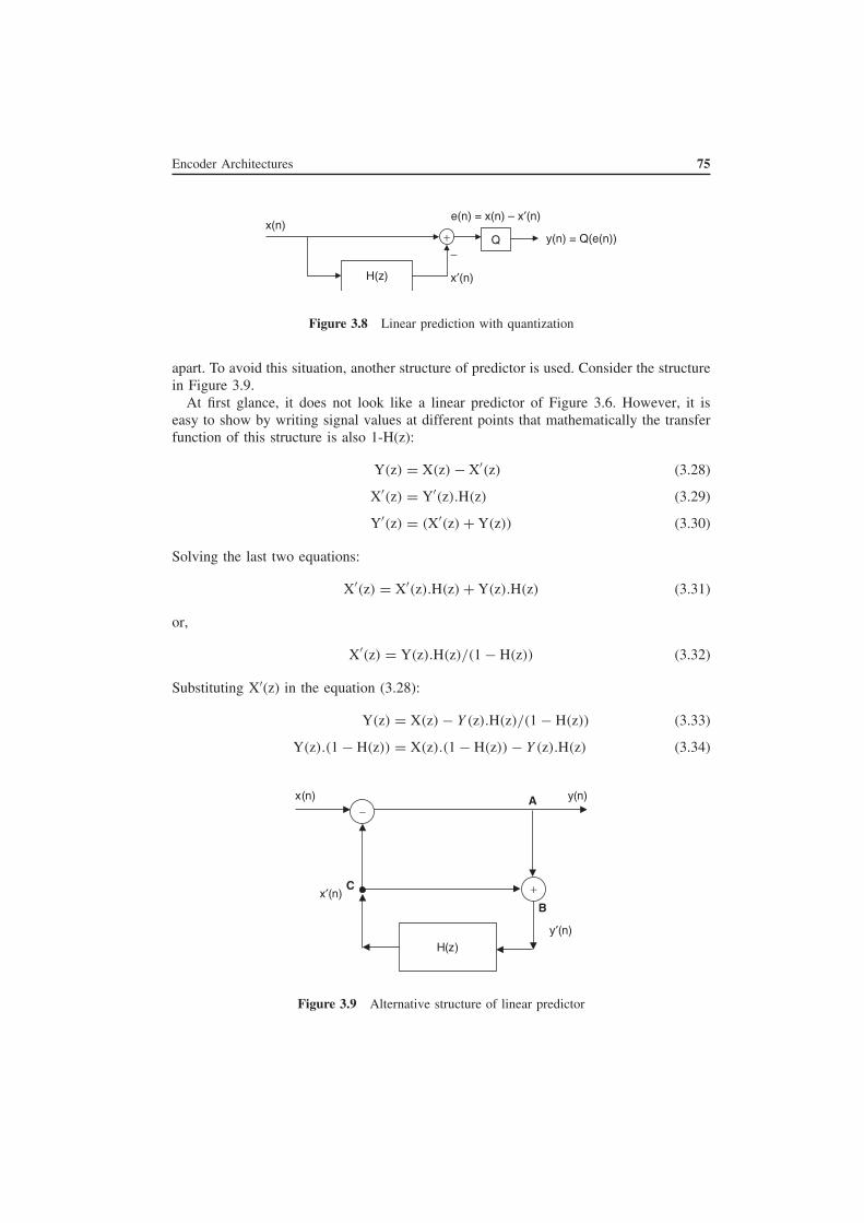
Encoder Architectures 75
x(n)e(n) = x(n) – x′(n)
H(z)
+
−
x′(n)
Q y(n) = Q(e(n))
Figure 3.8 Linear prediction with quantization
apart. To avoid this situation, another structure of predictor is used. Consider the structure
in Figure 3.9.
At first glance, it does not look like a linear predictor of Figure 3.6. However, it is
easy to show by writing signal values at different points that mathematically the transfer
function of this structure is also 1-H(z):
Y(z) = X(z) − X′(z) (3.28)
X′(z) = Y′(z).H(z) (3.29)
Y′(z) = (X′(z) + Y(z)) (3.30)
Solving the last two equations:
X′(z) = X′(z).H(z) + Y(z).H(z) (3.31)
or,
X′(z) = Y(z).H(z)/(1 − H(z)) (3.32)
Substituting X′(z) in the equation (3.28):
Y(z) = X(z) − Y (z).H(z)/(1 − H(z)) (3.33)
Y(z).(1 − H(z)) = X(z).(1 − H(z)) − Y (z).H(z) (3.34)
+
−
H(z)
x(n) y(n)
y′(n)
x′(n)
A
B
C
Figure 3.9 Alternative structure of linear predictor

76 Video Coding and Communications
+
− Q
H(z)
A
B
C
x(n) y(n)
Figure 3.10 DPCM encoder structure
or,
Y(z) = (1 − H(z)).X(z) (3.35)
which is the same as in equation (3.25).
Even though the structure in Figure 3.9 is mathematically the same as in Figure 3.6,
this provides an additional feature – it does not create drift between original input signal
and the decoded output in the presence of the quantizer. The quantizer in this structure
is introduced as shown in Figure 3.10.
It is easy to confirm that for the input provided in equation (3.26), output does not
drift far apart. Indeed, owing to quantization there is error in the decoded signal but it
is limited to the quantization step and large drift is not present. A useful way to analyze
the structure in Figures 3.9 and 3.10 is to note that the sub-structure between points A, B
and C (shown separately in Figure 3.11) is the same as the decoder shown in Figure 3.7.
The signal at point B is the same as the output of the decoder. Hence the prediction
x′(n) of x(n) (signal at C) is formed by using the past decoded values (at B), as opposed to
the past original input values (as in equation (3.22) and Figure 3.6). Therefore, whenever
the difference between the input and the predicted value starts to drift apart the difference
+
H(z)
A
B
C
Figure 3.11 Decoder sub-structure inside DPCM encoder shown in Figure 3.9

Encoder Architectures 77
+
− Q
H(z)
Q−1
Figure 3.12 DPCM encoder with quantizer and inverse quantizer
gets bigger and corrects the difference for the next sample and thus stops the input and
output from drifting. It is critical that this concept is understood.
Generally, scaling is also included as a part of quantization step. Therefore, both the
decoder and corresponding decoder sub-structure in the encoder contain the step of inverse
quantization (strictly speaking, it is actually an inverse scaling step). Therefore the encoder
and decoder structures are as shown in Figures 3.12 and 3.13.
3.4.2 Hybrid Transform-DPCM Architecture
One of the drawbacks of the DPCM style of encoder is that it does not allow one to fully
exploit the properties of the human visual system. The human visual system is less sen-
sitive to higher and diagonal frequencies and the DPCM encoder described above works
in the spatial domain. Therefore a hybrid transform-DPCM structure was first standard-
ized in H.261. At a high level, the motion compensated hybrid DCT-Transform-DPCM
encoder structure is as shown in Figure 3.14.
A two dimensional Discrete Cosine Transform (DCT) is taken before Quantization:
F(u, v) =2
NC(u) C(v)
N−1∑
x=0
N−1∑
y=0
f (x, y), cos
(
(2x + 1)uπ
2N
)
cos
(
(2y + 1)vπ
2N
)
(3.36)
where, x and y are the two dimensional locations of the pixels each ranging from 0 to
N−1, u, v are the two dimensional transform frequencies each ranging from 0 to N−1
and:
H(z−1)
+Q−1
Figure 3.13 DPCM decoder with inverse quantizer

78 Video Coding and Communications
+
− Q
Spatial / Temporal Prediction
DCT−1
DCT
Q−1
Variable Length Lossless Coding
Figure 3.14 Hybrid transform-DPCM structure
C(u), C(v) =
1√
2for u = 0, v = 0
1 otherwise
The quantization is now done in the transform domain. The characteristics and frequency
response of the human visual system are taken into account during the quantization
step. Higher and diagonal frequencies are quantized more than the lower frequencies.
The chroma component is quantized more heavily than the luma component. Note that
the international standards such as MPEG2 and AVC/H.264 (see Chapter 5) specify the
decoder behavior. Therefore, only the inverse cosine transform is specified. Equation
(3.36) provides the forward transform that an encoder should use to provide the least pos-
sible distortion in the decoded video. However, both the forward and inverse transform
contain irrational numbers. The standards also specify what level of precision decoders
are required to have and how they will convert real numbers to integers within a specified
range. Bit stream syntax also specifies the range of coefficients which encoders can use.
After the quantization of two dimensional DCT coefficients, they are scanned out in
a zig-zag pattern as a one dimensional signal. This one dimensional signal is passed
through the lossless Variable Length Codec (VLC). One dimensionally scanned transform
coefficients tend to have long strings of zeroes due to the quantization step. The lossless
coders are designed to be very efficient in removing those strings and compress the
scanned coefficients with great efficiency.
Overall, the hybrid DCT-transform-DPCM structure is shown in Figure 3.14. This
figure also illustrates that the prediction in these codecs is a three dimensional (spatial
and temporal) prediction where the estimated value of a current pixel is predicted from the
neighboring pixels in the same picture as well as the pixels in other pictures. Figure 3.15
depicts the high level structure of the corresponding decoder.
The basic structure of the encoder and the decoder remained the same in MPEG-1,
MPEG-2, MPEG-4 Part 2 (Simple Profile and Advanced Simple Profile) and AVC/H.264.
However, the accuracy of the predictions increased significantly.
It should be noted that the other profiles, besides Simple Profile (SP) and Advanced
Simple Profile (ASP), of MPEG-4 Part2 included object based coding algorithms and had

Encoder Architectures 79
Spatial / Temporal Prediction
Variable LengthDecoder
+Q−1DCT−1
Figure 3.15 Hybrid DCT-transform-DPCM decoder structure
different encoder and decoder structures. However, those algorithms and profiles have
not yet been deployed successfully in commercial applications. Those types of algorithms
may be adopted in future video coding standards and applications.
Why DCT?
It is well known that the DCT transform of a region of a picture gives coefficients that are
centered more around DC than other transforms such as the Discrete Fourier Transform
(DFT) and Hadamard Transform [13]. One way to look at the time limited DFT with N
samples is as a transform of a signal that is repeated periodically for every N sample.
So, if a one dimensional signal is as shown in Figure 3.16 then DFT corresponds to the
Fourier transform of a signal as shown in Figure 3.17.
Similarly, N sample DCT is the transform of the signal that is mirrored at the Nth
sample and then that mirrored pair is periodically repeated, as shown in Figure 3.18 for
the signal in Figure 3.16.
Therefore, for a signal that is not periodic in nature, one side of the signal is at a different
level than on the other side and the discontinuity in the repeated signal (Figure 3.18) is
smaller than that for DFT. This results in smaller higher frequency components. In the
early days of the video compression, the composite NTSC signal was sometimes sampled
and compressed directly (this was sometimes also called D-2 format). As the composite
signal consisted of sinusoidal chrominance carrier, DFT was used in place of DCT.
3.4.3 A Typical Hybrid Transform DPCM-based Video Codec
We next describe the hybrid transform-DPCM architecture in more detail. This is also
known as the Motion-Compensated Discrete Cosine Transform (MC-DCT) paradigm for
video compression. When specific details are given, they are based on the H.263 video
compression standard [15]. H.263 was chosen as a representative example of classic hybrid
transform-DPCM video coding. The latest digital video compression standard AVC/H.264
is described in Chapter 5.
In motion-compensated video compression, what we try to do is code the motion that
is present in the scene. Figure 3.19 shows an object (a circle) that appears in three
consecutive frames, but in different places. In this very simple case where the only
Figure 3.16 Signal to be transformed

80 Video Coding and Communications
Figure 3.17 Underlying assumption about the signal corresponding to DFT
Figure 3.18 Underlying assumption about signal corresponding to DCT
object in the picture is a circle, we only need to code this object in the first frame and
just code its motion in subsequent frames. This will lead to a much smaller number
of bits to represent the sequence than required if each frame is coded independently.
However, most video sequences are not so simple. Thus, more elaborate methods have
been invented to code the motion efficiently and compensate for the fact that objects and
background can appear and disappear from the scene. The motion estimation problem is a
challenging one. Although the motion is three-dimensional, we are only able to observe its
two-dimensional projection onto each frame. In addition, most motion estimators assume
that pure translation can describe the motion from one frame to the next. Because the
estimation of the motion is imperfect, we should also code the error that remains after
we compensate for the motion.
The first frame in the video sequence is coded independently, just like a regular image.
This is called an Intra frame. The compression is done as follows: First, the image is
divided into blocks (usually of size 8 × 8) and the discrete cosine transform (DCT ) of
each block is taken. The DCT maps each block to another 8 × 8 block of real number
t−1 t t+1
Figure 3.19 Motion-compensated video compression encodes the motion that is present in the
scene

Encoder Architectures 81
coefficients. This is done to decorrelate the pixels. Then, the DCT coefficients are quan-
tized. That is, they are represented by a finite set of values, rather than the whole
set of real numbers. Clearly, information is lost at this point. Finally, the quantized
coefficients are coded into bits using a lossless variable length coder and the bits are
transmitted.
After the first frame, subsequent frames are usually coded as Inter frames . That is,
interpicture prediction is used. This technique uses the same concept as differential pulse
code modulation. A prediction image is formed based on the previously reconstructed
frame and some information on the relationship between the two frames, which is provided
by the motion vectors. The difference between the actual frame and the prediction is then
coded and transmitted.
At the beginning of the transmission of an Inter frame, the picture is divided into
blocks (usually of a size 16 × 16). Unless there is a scene change in the picture, we
expect that each of the blocks in the current picture is similar to another 16 × 16 block
in the previously reconstructed frame. Clearly, these two blocks do not have to be in the
same spatial position. Thus, the coder uses a technique called block matching to identify
the block in the previous frame that best matches the block in the current frame. The
search is performed in the vicinity of the block in the current frame. Block matching
returns a vector that shows the relative spatial location of the best matching block in
the previous frame. This vector is called the motion vector . Thus, we obtain a motion
vector for each 16 × 16 block in the current frame. Now, we can obtain a prediction
of the current frame using the previously reconstructed frame and the motion vectors.
The prediction for each block of the current frame will be the block which is pointed
to by the corresponding motion vector. Then, the prediction error – that is, the differ-
ence between the actual frame and the prediction – is coded using a method similar to
the one described above for the Intra frames. The prediction error is transmitted along
with the motion vectors. The decoder reconstructs the prediction error and builds the
prediction image using the previous frame and the motion vectors. Finally, it produces
the reconstructed frame by adding the prediction error to the predicted frame. If the pre-
diction is good, we expect that the coding of the prediction error will require far less
bits than the coding of the original picture. However, in some cases, the prediction for
some blocks fails. This is the case when new objects are introduced in the picture or new
background is revealed. In that case, certain blocks or the entire picture can be coded in
Intra mode.
The basic structure of a motion-compensated DCT-based video codec is shown in
Figure 3.20. It can be seen that it is very similar in principle to a Differential Pulse
Code Modulation (DPCM) system. The switch indicates the choice between Intra and
Inter pictures or macroblocks. In the Intra case, the DCT of the image is taken and the
coefficients are quantized. In the Inter case, the difference between the predicted and
the actual picture is transmitted along with the motion vectors. It can be seen from the
picture that the encoder actually includes the decoder. This is because the prediction
has to be made using information that is available to the decoder. Thus, every encoded
frame has to be decoded by the coder and be used for the prediction of the next frame
instead of the original frame, since the actual frame is not available to the decoder.
Finally, in both the Intra and Inter cases, the quantized coefficients are variable length
coded.

82 Video Coding and Communications
One frame Delay
MotionCompensation
MotionEstimation
Inter
Inter
Intra
Intra
V
Video inDCT
DCT−1
Q q
Decoder
Q−1
V
+
+
−
−
Figure 3.20 The basic structure of a motion-compensated DCT-based video encoder
3.4.4 Motion Compensation
The motion vectors are typically coded differentially due to their redundancy. The dif-
ference between the actual motion vector and a predicted motion vector is coded and
transmitted. The decoder obtains the actual motion vector by adding the transmitted vec-
tor difference to the predicted vector. In H.263, the predicted vector is the median value
of three candidate predictors MV1, MV2, and MV3. The candidate predictors are deter-
mined as shown in Figure 3.21. Normally, MV1 is the previous motion vector, MV2
is the above motion vector and MV3 is the above right motion vector. However, there
are certain exceptions: Candidate predictor MV1 is set to zero if the corresponding mac-
roblock is outside the picture. The candidate predictors MV2 and MV3 are set to MV1
if the corresponding macroblocks are outside the picture. Finally, we check if the above
right macroblock is outside the picture. In that case, MV3 is set to zero.
MV2
MVMV1
MV3
Figure 3.21 The candidate predictors for the differential coding of the motion vectors

Encoder Architectures 83
A positive value of the horizontal or vertical component of a motion vector indicates
that the prediction is based on pixels in the referenced frame that are spatially to the right
or below the pixels being predicted.
A video compression standard does not specify how the motion vectors are determined.
The standard essentially specifies the decoder and a valid bit stream. It is up to the coder
to decide on issues such as the determination of the motion vector, mode selection, and
so on.
3.4.5 DCT and Quantization
A separable two-dimensional discrete cosine transform (DCT) of size 8 × 8 is taken for
each block using the following formula:
F(u, v) =1
4C(u)C(v)
7∑
x=0
7∑
y=0
f (x, y) cos[π(2x + 1)u/16] cos[π(2y + 1)v/16],
(3.37)
with u, v, x, y = 0, 1, 2, . . . , 7, where:
C(u) =
{
1/√
2 if u = 0
1 otherwise,(3.38)
C(v) =
{
1/√
2 if v = 0
1 otherwise,(3.39)
x, y are the spatial coordinates in the original block domain and u, v are the coordinates
in the transform domain.
For INTRA blocks, the DCT of the original sampled values of Y, Cb and Cr are taken.
For INTER blocks, the DCT of the difference between the original sampled values and
the prediction is taken.
Up to this point, no information has been lost. However, as noted earlier, in order
to achieve sufficient compression ratios, some information needs to be thrown away.
Thus, the DCT coefficients have to be quantized. For example, in H.263, the quantization
parameter (QP ) is used to specify the quantizer. QP may take integer values from 1 to 31.
The quantization step size is then 2 × QP. QP has to be transmitted along with the
quantized coefficients. The following definitions are made:
• /: Integer division with truncation toward zero.
• //: Integer division with rounding to the nearest integer.
Thus, if COF is a transform coefficient to be quantized and LEVEL is the absolute
value of the quantized version of the transform coefficient, the quantization is done as
follows.

84 Video Coding and Communications
For INTRA blocks (except for the dc coefficient):
LEVEL = |COF|/(2 × QP). (3.40)
For INTER blocks (all coefficients, including the dc):
LEVEL = (|COF| − QP/2)/(2 × QP) (3.41)
For the dc coefficient of an INTRA block:
LEVEL = COF//8 (3.42)
The quantized coefficients along with the motion vectors are variable length coded.
3.4.6 Procedures Performed at the Decoder
The following procedures are done at the source decoder after the variable length decoding
or arithmetic decoding:
• Motion compensation.
• Inverse quantization.
• Inverse DCT.
• Reconstruction of blocks.
Motion Compensation
The motion vector for each macroblock is obtained by adding predictors to the vector
differences. In the case of one vector per macroblock (i.e., when the advanced prediction
mode is not used), the candidate predictors are taken from three surrounding macroblocks,
as described previously. Also, half pixel values are found using bilinear interpolation, as
shown in Figure 3.22. In the case of H.263, the integer pixel positions are indicated by
the Xs and the half pixel positions are indicated by the Os. Integer pixel positions are
denoted with the letters A, B, C and D, and the half pixel positions are denoted with the
X
X
O O
X
X
O
A B
a b
c
C D
d
Figure 3.22 Half-pixel prediction is done using bilinear interpolation

Encoder Architectures 85
letters a, b, c and d. It should be noted that pixel A is the same as pixel a. Then, the half
pixel values are:
a = A (3.43)
b = (A + B+1)/2 (3.44)
c = (A + C+1)/2 (3.45)
d = (A + B + C + D+2)/4 (3.46)
Inverse Quantization
It should be pointed out that the term ‘inverse quantization’ does not imply that the
quantization process is invertible. The quantization operation is clearly not invertible.
This term simply implies the process of obtaining the reconstructed transform coefficient
from the transmitted quantization level. Thus, if COF’ is the reconstructed transform
coefficient and LEVEL is the absolute value of the quantized version of the transform
coefficient, the inverse quantization is done as follows for the example of H.263:
For INTRA blocks and INTER blocks, except for the dc coefficient:
|COF′| = 0 if LEVEL = 0 (3.47)
Otherwise:
|COF′| = 2 × QP × LEVEL + QP if QP is odd, (3.48)
|COF′| = 2 × QP × LEVEL + QP − 1 if QP is even. (3.49)
The sign of COF is then added to obtain |COF′|:
COF′ = Sign(COF) × |COF′| (3.50)
For the dc coefficient of an INTRA block:
COF′ = LEVEL × 8 (3.51)
Inverse DCT
After inverse quantization, the resulting 8 × 8 blocks are processed by a separable two-
dimensional inverse DCT of size 8 × 8. The output from the inverse transform ranges
from – 256 to 255 after clipping to be represented with 9 bits.
The Inverse DCT is given by the following equation:
f (x, y) =1
4
7∑
u=0
7∑
v=0
C(u)C(v)F (u, v) cos[π(2x + 1)u/16] cos[π(2y + 1)v/16] (3.52)

86 Video Coding and Communications
with u, v, x, y = 0, 1, 2, . . .,7, where:
C(u) =
{
1/√
2 if u = 0
1 otherwise,(3.53)
C(v) =
{
1/√
2 if v = 0
1 otherwise,(3.54)
x, y are the spatial coordinates in the original block domain and u, v are the coordinates
in the transform domain.
Reconstruction of Blocks
After the inverse DCT, a reconstruction is formed for each luminance and chrominance
block. For INTRA blocks, the reconstruction is equal to the result of the inverse transfor-
mation. For INTER blocks, the reconstruction is formed by summing the prediction and
the result of the inverse transformation. The transform is performed on a pixel basis.
3.5 Wavelet-Based Video Compression
We next present the basics of video compression using the Discrete Wavelet Transform
(DWT). The DWT has been very successful in video compression and DWT-based codecs
have been proven to outperform the DCT-based ones [16, 17]. Also, the JPEG-2000
standard is wavelet-based [18]. These image codecs, besides offering good compression,
also offer efficient SNR scalability . A scalable encoder produces a bitstream that can
be partitioned into layers. One layer is the base layer and can be decoded by itself and
provide a basic signal quality. One or more enhancement layers can be decoded along
with the base layer to provide an improvement in signal quality. For image coding, the
improvement will be in terms of image quality. Thus, the PSNR of the image will be
increased (SNR scalability). For video coding, the improvement may also be in terms
of spatial resolution (spatial scalability) or temporal resolution (temporal scalability).
DWT-based image codecs produce a bitstream that can be partitioned into arbitrary layers.
Thus, the bitstream can be ‘chopped-off’ at any point and the first part of it can be decoded.
Furthermore, the image quality of this first part of the bitstream will typically be better
than that of non-scalable DCT-based coding at the same bit rate.
The efficient compression and scalability of DWT-based image codecs compared to
their DCT-based counterparts has inspired research on wavelet-based video compression.
However, so far, no video compression standard is wavelet-based, except for some limited
use of wavelet-based coding for intra frames in standards such as MPEG-4 [19]. We will
next attempt to discuss some of the problems and challenges involved in applying the
DWT to video coding. We will assume that the reader has some basic knowledge on
wavelet based image coding. More information can be found in [16–18].
Figure 3.23 shows a block diagram for a DWT-based video encoder. It can be seen
that such an encoder is very similar to a classic motion-compensated DCT-based encoder.
Motion estimation and compensation are done in the spatial domain and the encoding of

Wavelet-Based Video Compression 87
DWTVideo In +
++
+
+
−
EmbeddedEncoder
EmbeddedDecoder
MotionCompensation
MotionEstimation
MVs
Figure 3.23 A DWT -based video encoder with motion estimation and compensation in the spatial
domain
the prediction error is done using DWT instead of DCT using an encoder like SPIHT, EZW
or JPEG-2000. Such a codec does not outperform DCT-based codecs. The main reason
is the following: Motion estimation and compensation is done on a block basis. Thus,
the prediction error will inevitably have discontinuities along block edges. In DCT-based
codecs, the DCT is taken along blocks as well (typically of size 8 × 8) and the DCT
block edges coincide with the discontinuities of the prediction error. Thus, there are no
discontinuities that are due to the block-based motion compensation in the 8 × 8 DCT
blocks. On the other hand, the DWT is taken on the whole image (in this case, the
prediction error) instead of blocks. Thus, the encoder will have to spend bits to encode
these discontinuities and this reduces the efficiency of the codec in Figure 3.23.
Figure 3.24 shows another DWT-based video encoder. Compared to the encoder in
Figure 3.23, the encoder in Figure 3.24 performs motion estimation in the DWT domain
instead of the spatial domain. Thus, the prediction error is already in the DWT domain and
just needs to be encoded into a bitstream. This eliminates the efficiency problems that
were due to the discontinuities that were present in the prediction error when performing
block-based motion compensation in the spatial domain. However, another problem arises,
which is due to the fact that the DWT is not shift-invariant. Assuming a one-dimensional
signal and one level of decomposition, the DWT corresponds to filtering the signal using
a high-pass and a low-pass discrete-time filter and sub-sampling the outputs by a factor of
two. A system is shift-invariant if a shift in its input corresponds to a shift in its output. In
DWT, if we shift the input by, say, one sample, we will not get the output of the original
signal shifted by one sample due to the fact that the sub-sampling will discard different
samples in this case. Thus, the DWT is not shift-invariant. This poses a problem when
performing motion estimation and compensation in the DWT domain. Let us assume a
video sequence consisting of two frames. The second frame is basically the first frame
shifted by one pixel in the horizontal direction. If motion estimation and compensation

88 Video Coding and Communications
DWTVideo In +
++
+
+
−
EmbeddedEncoder
EmbeddedDecoder
MotionCompensation
MotionEstimation
MVs
Figure 3.24 A DWT-based video encoder with motion estimation and compensation in the
wavelet domain
are performed in the spatial domain, the second frame can be predicted perfectly from
the first (except of course for the first pixel column of the image). However, if motion
estimation and compensation are performed in the DWT domain, the second frame cannot
be perfectly predicted from the first, exactly because the DWT is not shift-invariant.
Thus, motion estimation and compensation are less efficient when performed in the DWT
domain. Another way of looking at it is that the DWT spatial sub-bands have a lower
resolution than the original video frames (due to the sub-sampling), thus the motion
estimation and compensation is not as efficient.
A solution to the problem above is to use the Overcomplete Discrete Wavelet Trans-
form (ODWT) instead of the DWT. The ODWT corresponds to the DWT without the
sub-sampling. Thus, the ODWT representation of a signal has more samples than the
DWT and the original signal, that’s why it is called overcomplete. Since the DWT is by
itself sufficient to represent a signal, it is always possible to derive the ODWT from the
DWT. Thus, it is possible to convert the reference frame from the DWT to the ODWT and
predict the DWT of the current frame from the ODWT of the previous (reference) frame.
Clearly, the prediction error will be in the DWT domain. Thus, the use of the ODWT
instead of the DWT does not increase the number of pixels to be encoded. Figure 3.25
illustrates the OWDT.
The use of the ODWT improves compression efficiency significantly. Since we are using
image codecs such as SPIHT or JPEG-2000 for the encoding of the prediction error, we
might think that we have efficient scalability, just like when applying these codecs to
image compression. Unfortunately, this is not the case. Figure 3.26 illustrates why. If
frame k is encoded using the full bitstream but is decoded using part of the bitstream,
the decoder will have a different frame k than the encoder. Recall that the encoder has
a decoder in it so that encoder and decoder have the same reference frame. This would
be impossible in this case. Thus, the quality of frame k+1 and subsequent frames will
deteriorate due to the fact that different reference frames will be used at the encoder and
decoder. We will refer to this discrepancy between encoder and decoder as drift . Drift

Wavelet-Based Video Compression 89
DWT
ODWT
ORIGINAL FRAME
Figure 3.25 An illustration of Overcomplete Discrete Wavelet Transform (ODWT )
can be avoided by using only base layer information for prediction. Thus, encoder and
decoder will always have the same reconstructed frame to use as reference. However, this
results in a reduction of compression efficiency because the reference frames will be of
lesser quality, thus, more information will have to be encoded with the prediction error,
thus resulting in an increase of the number of bits to be transmitted. For these reasons,
initial efforts towards applying wavelets to video compression were not very successful.
A way of avoiding drift problems is to utilize a 3D wavelet transform, the third dimen-
sion being time. Thus, a three dimensional signal is constructed by concatenating a group
of frames (GOFs) and a three-dimensional DWT is applied. Then, the resulting signal
in the DWT domain can be encoded temporal sub-band by temporal sub-band using,
for example, SPIHT, or it can be encoded all at once using a technique like 3D-SPIHT
[20]. Then, the resulting bitstream will have the same nice SNR scalability properties
that DWT-based image coding has. However, if the DWT is applied in a straightforward
fashion without any motion compensation, the encoding will not take full advantage of
the temporal redundancy in the video signal.
Encoder
Base
ME/MC MC
Drift
Fkenc
F(k+1)encF(k+1)dec
Fkenc ≠ Fkdec
Enhancement Base Enhancement
Decoder
Fkdec
Figure 3.26 Illustration of the drift problems of the wavelet-based codecs of Figure 3.23 and
Figure 3.24

90 Video Coding and Communications
The main theoretical development that promises efficient 3D wavelet-based video
codecs with perfect invertibility is motion compensated temporal filtering (MCTF)
using lifting, which was first introduced in [21, 22]. MCTF may be performed in two
ways:
• Two-dimensional spatial filtering followed by temporal filtering (2D+t) [23–27].
• Temporal filtering followed by two-dimensional spatial filtering (t+2D) [28–31].
In the case of 2D+t motion compensated temporal filtering, the motion estimation and
compensation is performed in the ODWT domain. Figure 3.27 illustrates 2D+t motion
compensated temporal filtering while Figure 3.28 illustrates t+2D motion compensated
temporal filtering.
The resulting wavelet coefficients can be encoded using different algorithms like
3D-SPIHT [20] or 3D-ESCOT [32]. Several enhancements have been made recently
to the MCTF schemes presented either by introducing longer filters or by optimizing
the operators involved in the temporal filter [23, 27, 28, 33]. Recently, a JPEG2000-
compatible scalable video compression scheme has been proposed that uses the 3/1 filter
for MCTF [34].
Though 3D schemes offer drift-free scalability with high compression efficiency, they
introduce considerable delay, which makes them unsuitable for some real time video
applications like tele-conferencing. In contrast to 2D methods, frames cannot be encoded
one by one but processing is done in groups of frames. Thus, a certain number of frames
must be available to the encoder to start encoding. The number of frames required depends
on the filter length. Similarly, the group of frames must be available at the receiver before
decoding can start. Thus, 3D video coding schemes offer better performance but also relax
the causality of the system.
3.5.1 Motion-Compensated Temporal Wavelet Transform Using Lifting
Lifting allows for the incorporation of motion compensation in temporal wavelet trans-
forms while still guaranteeing perfect reconstruction. Any wavelet filter can be imple-
mented using lifting. Let us consider as an example the Haar wavelet transform:
DWT
DWTto
ODWT
MotionEstimation
TemporalSubbands
SubbandCoder
Bitstream
MCTF
Figure 3.27 Illustration of 2D+t motion compensated temporal filtering

Wavelet-Based Video Compression 91
MCTF
MotionEstimation
TemporalSubbands
SubbandCoder
Bitstream
SpatialDecomposition
Figure 3.28 Illustration of t+2D motion compensated temporal filtering
hk[x, y] = f2k+1[x, y] − f2k[x, y] (3.55)
lk[x, y] =1
2{f2k[x, y] + f2k+1[x, y]} (3.56)
where fk[x, y] denotes frame k and hk[x, y] and lk[x, y] represent the high-pass and
low-pass temporal sub-band frames. The lifting implementation of the above filter cal-
culates the high-pass temporal sub-band first and then uses it in order to calculate the
low-pass temporal sub-band:
hk[x, y] = f2k+1[x, y] − f2k[x, y] (3.57)
lk[x, y] = f2k[x, y] +1
2hk[x, y] (3.58)
Using lifting, the Haar filter along the motion trajectories with motion compensation can
be implemented as:
hk[x, y] = f2k+1[x, y] − W2k→2k+1(f2k[x, y]) (3.59)
lk[x, y] = f2k[x, y] +1
2W2k+1→2k(hk[x, y]) (3.60)
where Wi→j (fi) denotes the motion-compensated mapping of frame fi into frame fj .
Thus, the operator Wi→j (.) gives a per pixel mapping between two frames and this is
applicable to any motion model.
In the case of the biorthogonal 5/3 wavelet transform, the analysis equations using
motion compensated lifting are
hk[x, y] = f2k+1[x, y] −1
2{W2k→2k+1(f2k[x, y]) + W2k+2→2k+1(f2k+2[x, y])} (3.61)
lk[x, y] = f2k[x, y] +1
4{W2k−1→2k(hk−1[x, y]) + W2k+1→2k(hk[x, y])} (3.62)
In the lifting operation, the prediction residues (temporal high pass sub-bands) are used
to update the reference frame to obtain a temporal low sub-band. We will refer to this as
the update step (equation (3.62)) in the following discussion.

92 Video Coding and Communications
If the motion is modeled poorly, the update step will cause ghosting artifacts to the low
pass temporal sub-bands. The update step for longer filters depends on a larger number of
future frames. If a video sequence is divided into a number of fixed sized GOFs that are
processed independently, without using frames from other GOFs, high distortion will be
introduced at the GOF boundaries for longer filters. When longer filters based on lifting
are used with symmetric extension, the distortion will be in the range of 4–6 dB (PSNR)
at the GOF boundaries irrespective of the motion content or model used [27, 28]. Hence,
to reduce this variation at the boundaries, we need to use frames from past and future
GOFs. Thus, it is observed that the introduced delay (in frames) is greater than the number
of frames in the GOF. The encoding and decoding delay will be very high, as the encoder
has to wait for future GOFs. In [28], the distortion at the boundaries for the 5/3 filter is
reduced to some extent by using a sliding window approach. But this clearly introduces
delay both at the encoder and at the decoder. We should note that, even when the delay
is high, if the motion is not modeled properly, then the low pass temporal sub-bands will
not be free from ghosting artifacts.
By skipping entirely the update step for 5/3 filter [31, 35], the analysis equations can
be modified as:
hk[x, y] = f2k+1[x, y] −1
2{W2k→2k+1(f2k[x, y]) + W2k+2→2k+1(f2k+2)[x, y]} (3.63)
lk[x, y] = f2k[x, y] (3.64)
We refer to this filter set as the 3/1 filter.
Filters without update step will minimize the dependency on future frames thereby
reducing the delay. Also, the low pass temporal sub-bands are free from ghosting artifacts
introduced by the update step. Hence, by avoiding the update step, we get high quality
temporal scalability with reduced delay. But at full frame rate resolution, the 3/1 filter
suffers in compression efficiency compared to the 5/3 filter.
In 3D coding schemes, a high level of compression efficiency is achieved by applying
a temporal filter to a group of frames. The number of frames in a buffer will increase with
the length of the filter and the number of temporal decomposition levels. This introduces
a delay both at the encoder and decoder. As mentioned earlier, the 3/1 filter offers less
delay than the 5/3 filter at the expense of compression efficiency. A family of temporal
filters with the following requirements has been proposed [26]:
• Any GOF length N can be used.
• Each GOF can be processed independently, without need for frames from neighboring
GOFs.
• Motion compensated temporal filtering is used.
• Compression efficiency of the proposed filter set should be at least competitive with
the 5/3 filter.
Thus, a filter set is proposed that is defined by the filter length N and the number of
lifting steps involved (S). The filter length N here refers to the number frames being
filtered. We refer to the filter set as (N, S) temporal filter. The number of frames N can
vary from two to any number and need not be in some power of two. Unlike 5/3 and other
longer filters, the proposed (N, S) filter can be processed independently (without reference

Wavelet-Based Video Compression 93
to other GOFs) and thus finite fixed size GOFs can be created without introducing high
distortions at the boundary. Any combination of (N, S) filters can be chosen to achieve
the given delay requirements.
A detailed explanation of the (N,S ) filter set is beyond the scope of this chapter. More
information can be found in [26]. It should be pointed out that, unlike the 5/3 and 3/1
temporal filters, the (N, S) temporal filter does not correspond to a temporal wavelet
transform.
Figure 3.29 shows an illustration of the (5, 2) filter with the update step. It can be seen
that the GOF consists of five frames and there are two lifting steps (levels of temporal
decomposition). As in all (N,S) filters, the first frame in the GOF is not updated. Thus,
low pass temporal sub-bands L10 and L2
0 (where the superscript corresponds to the level of
decomposition) are identical to the original frame F0. However, sub-bands L12 and L2
1 are
not identical to F4 due to the update steps. The following temporal sub-bands will need
to be encoded and transmitted: L20,H
10 ,H 2
0 ,H 11 , L2
1. The low pass temporal sub-bands are
analogous to intra frames in motion-compensated DCT-based video coding, whereas the
high pass temporal sub-bands are analogous to inter frames. Of course, if update steps are
used, the low pass temporal sub-bands are not identical to the original frames. A (N,S)
temporal filter produces two low pass temporal sub-bands and N -2 high pass temporal
sub-bands. Since low pass sub-bands have more information and require more bits to
encode, we would prefer to have only one low pass sub-band per GOF. It is possible to
concatenate another temporal filter to the (N,S) filter in order to obtain a GOF with only
one low pass temporal sub-band [26].
Figure 3.30 illustrates the (5, 2) temporal filter for the case without an update step. Also,
actual frames and temporal sub-bands are shown. Now, both the first and fifth frames of
the GOF are not updated and are identical to the original video frames. By looking at the
Fb
H10
L10
L11 L
12
L20
H20
L21
H11
F1 F2 F3 F4
−0.5
−0.5
S = 1
S = 2
−0.5−0.5
w1 w3
w3
w2
−0.5
−0.5
Figure 3.29 Illustration of the (5, 2) temporal filter (with update step)

94 Video Coding and Communications
Figure 3.30 Illustration of the (5, 2) temporal filter (without update step)
temporal sub-bands of Figure 3.30, it becomes clear that low pass frames are analogous
to intra frames and high pass frames are analogous to inter frames.
References
1. BT 601 Recommendation ITU-R BT.601-6, Studio encoding parameters of digital television for standard
4:3 and wide-screen 16:9 aspect ratios, Year 2007.
2. J. Keith, “Video demystified, 4th Edition (Demystifying Technology),” Elsevier Inc., 2005.
3. Schanda, J., “Colorimetry: Understanding the CIE System.” John Wiley & Sons, Inc, US, 2007.
4. ISO/IEC JTC 1 and ITU-T, “Generic coding of moving pictures and associated audio information – Part
2: Video,” ISO/IEC 13818-2 (MPEG-2) and ITU-T Rec. H.262, 1994 (and several subsequent amendments
and corrigenda).
5. AVC ISO/IEC JTC 1 and ITU-T, “Advanced video coding of generic audiovisual services,” ISO/IEC
14496-10 (MPEG-4 Part 10) and ITU-T Rec. H.264, 2005 (and several subsequent amendments and
corrigenda).
6. ISO/IEC JTC 1, “Coding of moving pictures and associated audio for digital storage media at up to about
1,5 Mbit/s – Part 2: Video,” ISO/IEC 11172 (MPEG-1), Nov. 1993.
7. C. Poynton, A Technical Introduction to Digital Video, John Wiley & Sons, US, 1996.
8. T.M. Cover and J. A. Thomas, Elements of Information Theory , John Wiley & Sons, Inc, US, 1991.
9. R. G. Gallager, Information Theory and Reliable Communication , John Wiley & Sons, Inc, US, 1968.
10. Y. Wang, J. Ostermann and Y.-Q Zhang, Video Processing and Communications , Prentice-Hall, 2002.
11. A. Papoulis and S. U. Pillai, Probability, Random Variables and Stochastic Processes, McGraw-Hill, 2002.
12. K. Sayood, Introduction to Data Compression , Morgan Kaufmann, 1996.
13. A. N. Netravali and B. G. Haskell, “Digital Pictures – Representation and Compression,” Plenum Press,
June 1989.

References 95
14. A. V. Oppenheim, R. W. Schafer and J. R. Buck, “Discrete-Time Signal Processing, 2nd Edition,” Prentice
Hall, December 1998.
15. ITU-T Rec. H.263, Video Codec for low bit rate communication, 1996.
16. A. Said and W. Pearlman, “A new, fast, and efficient image codec based on set partitioning in hierarchical
trees”, IEEE Transactions on Circuits and Systems for Video Technology , Vol. 6, pp. 243–50, June 1996.
17. J. M. Shapiro, “Embedded image coding using zerotrees of wavelet coefficients,” IEEE Transactions on
Signal Processing , Vol. 41, No. 12, pp. 3445–62, 1993.
18. C. Christopoulos, A. Skodras, and T. Ebrahimi, “The JPEG-2000 still image coding system: an overview,”
IEEE Transactions on Consumer Electronics , Vol. 46, No. 4, pp. 1103–27, 2000.
19. MPEG4 video group, “Core experiments on multifunctional and advanced layered coding aspects of
MPEG-4 video”, Doc. ISO/IEC JTC1/SC29/WG11 N2176, May 1998.
20. B.-J. Kim, Z. Xiong, and W. A. Pearlman, “Low bit-rate scalable video coding with 3-D set partitioning
in hierarchical trees (3-D SPIHT),” IEEE Transactions on Circuits and Systems for Video Technology , Vol.
10, No. 8, pp. 1374–87, 2000.
21. B. Pesquet-Popescu and V. Bottreau, “Three-dimensional lifting schemes for motion compensated video
compression,” in Proc. IEEE International Conference on Acoustics, Speech and Signal Processing , Salt
Lake City, UT, 2001, pp. 1793–6.
22. A. Secker and D. Taubman, “Motion-compensated highly scalable video compression using an adaptive
3-D wavelet transform based on lifting,” in Proc. IEEE Conference on Image Processing , Thessaloniki,
Greece, 2001, pp. 1029–32.
23. Y. Andreopoulos, A. Munteanu, J. Barbarien, M. van der Schaar, J., and P. Schelkens, “In-band motion
compensated temporal filtering,” Signal Processing: Image Communication , Vol. 19, No. 7, pp. 653–73,
2004.
24. X. Li, “Scalable video compression via overcomplete motion compensated wavelet coding,” Signal Pro-
cessing: Image Communication , Vol. 19, No. 7, pp. 637–51, 2004.
25. V. Seran and L. P. Kondi, “Quality variation control for three-dimensional wavelet-based video
coders,” EURASIP Journal on Image and Video Processing , Volume 2007, Article ID 83068, 8 pages,
doi:10.1155/2007/83068.
26. V. Seran and L. P. Kondi, “New temporal filtering scheme to reduce delay in wavelet-based video coding,”
IEEE Transactions on Image Processing , Vol. 16, No. 12, pp. 2927–35, December 2007.
27. Y. Wang, S. Cui, and J. E. Fowler, “3D video coding using redundant-wavelet multihypothesis and
motion-compensated temporal filtering,” in Proceedings of IEEE International Conference on Image Pro-
cessing (ICIP ’03), Vol. 2, pp. 755–8, Barcelona, Spain, September 2003.
28. A. Golwelkar and J. W. Woods, “Scalable video compression using longer motion compensated temporal
filters,” in Visual Communications and Image Processing , Vol. 5150 of Proceedings of SPIE , pp. 1406–16,
Lugano, Switzerland, July 2003.
29. S. T. Hsiang and J. W. Woods, “Embedded video coding using motion compensated 3-D sub-band/wavelet
filter bank,” in Proceedings of the Packet Video Workshop, Sardinia, Italy, May 2000.
30. G. Pau, C. Tillier, B. Pesquet-Popescu, and H. Heijmans, “Motion compensation and scalability in
lifting-based video coding,” Signal Processing: Image Communication , Vol. 19, No. 7, pp. 577–600,
2004.
31. A. Secker and D. Taubman, “Lifting-based invertible motion adaptive transform (LIMAT) framework
for highly scalable video compression,” IEEE Transactions on Image Processing , Vol. 12, No. 12, pp.
1530–42, 2003.
32. J. Xu, S. Li and Y. Q. Zhang, “A wavelet codec using 3-D ESCOT,” in IEEE PCM , December 2000.
33. N. Mehrseresht and D. Taubman, “An efficient content adaptive motion compensation 3-D-DWT with
enhanced spatial and temporal scalability,” in Proc. IEEE International Conference on Image Processing ,
2004, Vol. 2, pp. 1329–32.
34. T. Andre, M. Cagnazzo, M. Antonini, and M. Barlaud, “JPEG2000-compatible scalable scheme
for wavelet-based video coding,” EURASIP Journal on Image and Video Processing , 2007, DOI:
10.1155/2007/30852.
35. M. van der Schaar and D. S. Turaga, “Unconstrained motion compensated temporal filtering (UMCTF)
framework for wavelet video coding,” in Proceedings of the IEEE International Conference on Acoustics,
Speech, and Signal Processing (ICASSP ’03), Vol. 3, pp. 81–4, Hong Kong, April 2003.

4
4G Wireless Communicationsand Networking
4.1 IMT-Advanced and 4G
Today, wireless technologies and systems which are claimed to be “4G” represent a market
positioning statement by different interest groups. Such claims must be substantiated
by a set of technical rules in order to qualify as 4G. Currently, the ITU (International
Telecommunications Union) has been working on a new international standard for 4G,
called IMT-Advanced, which is regarded as an evolutionary version of IMT-2000, the
international standard on 3G technologies and systems.
With the rapid development of telecommunications technologies and services, the num-
ber of mobile subscribers worldwide has increased from 215 million in 1997 to 946 million
(15.5% of global population) in 2001, as shown in Figure 4.1. It is predicted that by the
year 2010 there will be 1700 million terrestrial mobile subscribers worldwide. A substan-
tial portion of these additional subscribers is expected to be from outside the countries
that already had substantial numbers of mobile users by the year 2001. Figure 4.1 shows
the user trends of mobile and wireline telecommunications services and applications.
4G technologies can be thought of as an evolution of the 3G technologies which
are specified by IMT-2000. The framework for the future development of IMT-2000
and IMT-Advanced and their relationship to each other are depicted in Figure 4.2.
Systems beyond IMT-2000 will encompass the capabilities of previous systems. Other
communication relationships will also emerge, in addition to person-to-person, such as
machine-to-machine, machine-to-person and person-to-machine.
One of the unique features of 4G networks is that they will accommodate heteroge-
neous radio access systems, which will be connected via flexible core networks. Thus, an
individual user can be connected via a variety of different access systems to the desired
networks and services. The interworking between these different access systems in terms
of horizontal and vertical handover and seamless service provision with service negotiation
including mobility, security and QoS management will be a key requirement, which may
be handled in the core network or by suitable servers accessed via the core network. This
4G Wireless Video Communications Haohong Wang, Lisimachos P. Kondi, Ajay Luthra and Song Ci
© 2009 John Wiley & Sons, Ltd. ISBN: 978-0-470-77307-9

98 4G Wireless Communications and Networking
1800
1600
1400
1200
1000
800
600
400
200
01995 2000 2005 2010
Mobile subscribers
Wireline subscribers
Mobile Internet
Wireline Internet
Su
bscrip
tio
ns w
orld
wid
e (
mill
ion
s)
Figure 4.1 Global growth of mobile and wireline subscribers. Reproduced with kind permission
from ITU, 2008
optimally connected anywhere, anytime view could be realized by a network comprising
a variety of interworking access systems connected to a common packet-based core net-
work, as seen in Figure 4.3. Figure 4.4 illustrates a flexible and scalable environment
which can be used for the allocation of system capacity in a deployment area, where one
or more systems may be deployed according to need.
The timelines associated with these different factors are depicted in Figure 4.5. When
discussing the time phases for IMT-advanced, it is important to specify the time at which
the standards are completed, when spectrum must be available, and when deployment
may start. Currently, IMT-Advanced is still at the call-for-proposal stage.
IMT-Advanced has been developed to provide true end-to-end IP services to mobile
users at “anytime anywhere”. Although the standardization process is still ongoing, the
major design goals of 4G are quite certain, which are: 1) 4G will be all IP networks,
meaning that circuit switching will be eliminated in the next-generation cellular networks.
2) 4G will have a very high data rate. It is expected that 4G networks will be capable of
providing 100 Mbps data rate under high mobility, which is much faster than 3G. 3) 4G
will provide Quality of Service (QoS) and security to the end users, which has been
lacking in 3G. 4) IP-based multimedia services such as Voice over IP (VoIP) and video
streaming are expected to be the major traffic types in 4G. In this chapter, we will discuss
three major contenders for 4G technologies: 3GPP Long Term Evolution (LTE), WiMax
IEEE 802.16m and 3GPP2 Ultra Mobile Broadband (UMB).

LTE 99
Systems beyond IMT-2000 will encompassthe capabilities of previous systems
Mobility
High
Low
1 10 100 1000
Peak useful data rate (Mbits/s)
Denotes interconnection between systems via networks, which allowsflexible use in any environment without making users aware ofconstituent systems
Nomadic/local area access systems
Digital broadcast systems
Dark shading indicates existing capabilities, medium shading indicates enhancements toIMT-2000, and the lighter shading indicates new capabilities of systems beyond IMT-2000.
The degree of mobility as used in this Figure is described as follows: low mobility coverspedestrian speed, and high mobility covers high speed on highways or fast trains (60 km/h to~250 km/h, or more).
IMT-2000Enhanced
TMT-2000
New
mobile
access
Enhancement
New nomadic/localarea wireless access
New capabilitiesof systems beyondIMT-2000
Dashed line indicatesthat the exact datarates associated withsystems beyond IMT-2000are not yet determined
Figure 4.2 Illustration of capabilities of IMT-2000 and IMT-Advanced. Reproduced with kind
permission from ITU, 2008
4.2 LTE
LTE, which stands for 3rd Generation Partnership Project (3GPP) Long Term Evo-
lution, is one of the next major steps in mobile radio communications designed to
ensure competitiveness in a longer time frame, i.e. for the next 10 years and beyond.
The increasing usage of mobile data and newly-emerged applications such as Multi-
media Online Gaming (MMOG), mobile TV and streaming services has motivated the
3GPP to work on this standard. The aim of LTE is to improve the Universal Mobile
Telecommunications System (UMTS) mobile phone standard and provide an enhanced
user experience for next generation mobile broadband. LTE is planned to be introduced
in 3GPP Release 8.

100 4G Wireless Communications and Networking
Short rangeconnectivity
IMT-2000
RLANtype
Cellular2nd generation
Download channel Digitalbroadcast
Services andapplications
New radiointerface
Packet-basedcore network
WirelinexDSL
Otherentities
Figure 4.3 Future IMT-Advanced network, including a variety of potential interworking access
systems. Reproduced with kind permission from ITU, 2008
Distribution layer
Cellular layer
Hot spot layer
Personal network layer
Fixed (wired) layer X X X X X X X X X X X XX X X
Full coverageGlobal accessFull mobility
Full mobility
Not necessarily individual links
Full coverage and hot spotsGlobal roaming
Individual links
Local coverageHot spotsGlobal roamingLocal mobilityIndividual links
Short range communicationGlobal roamingIndividual links
Personal mobilityGlobal access
Horizontal: handover within a system
Vertical: handover between systems
Possible return channels
Figure 4.4 Illustration of complementary access systems. Reproduced with kind permission from
ITU, 2008

LTE 101
2000 2003 2006 2009 2012 2015
The sloped dotted lines indicate that the exact starting point of the particular subject can not yet be fixed
:Possible spectrum identification at WRC-07
:Possible wide deployment around the year 2015 in some countries*
IMT-2000and future
development
Other radiosystems
New elementsto offer newcapabilitiesof systems
beyondIMT-2000
Systems deployment*
Spectrum implementation
Visiondefinition
Requirementsdefinition
Standardsdevelopment
Standardsenhancement
Evolution/integration with otherradio systems
Systems deployment
Spectrum implementation
Enhancement and relateddevelopment of standards
Figure 4.5 Phases and expected timelines for IMT-Advanced. Reproduced with kind permission
from ITU, 2008
4.2.1 Introduction
The high-level LTE requirements for 3GPP radio-access technology include reduced
latency, higher user data rates, improved system capacity and coverage and reduced
costs for operators. Therefore, an evolution of the radio interface as well as the radio
network architecture should be considered. It was also recommended that the Evolved
UTRAN (E-UTRAN) should bring significant improvement so as to justify the standard-
ization effort and should avoid unnecessary options. The main advantages of LTE are
high throughput, low latency, plug and play, FDD and TDD in the same platform, supe-
rior end-user experience and simple architecture resulting in low Operating Expenditures
(OPEX). Furthermore, LTE also supports seamless connection to existing networks, such
as GSM, CDMA and HSPA.
The feasibility study on the UTRA and UTRAN Long Term Evolution was started in
December 2004, with the objective being “to develop a framework for the evolution of the
3GPP radio-access technology towards a high-data-rate, low-latency and packet-optimized
radio-access technology” [1, 2]. The study focused on supporting services provided from
the PS-domain, concerning the radio interface physical layer for both downlink and uplink,

102 4G Wireless Communications and Networking
the radio interface layers 2 and 3, the UTRAN architecture and RF issues. Furthermore,
the Next Generation Mobile Networks (NGMN) initiative provided a set of recommen-
dations for the creation of networks suitable for the competitive delivery of mobile
broadband services, with the goal of “to provide a coherent vision for technology evo-
lution beyond 3G for the competitive delivery of broadband wireless services” [1, 2].
The long-term objective of NGMN is to “establish clear performance targets, fundamen-
tal recommendations and deployment scenarios for a future wide area mobile broadband
network” [1, 2].
The goals of LTE include improving spectral efficiency, lowering costs, improving
services, making use of new spectrum and reframed spectrum opportunities and better
integration with other open standards. The architecture that results from this work is
called Evolved Packet System (EPS) and comprises Evolved UTRAN (E-UTRAN) on
the access side and Evolved Packet Core (EPC) on the core side. EPC is also known as
System Architecture Evolution (SAE) and E-UTRAN is also known as LTE.
As a result, the detailed requirements laid down for LTE can be found in the Table 4.1
[3]. Generally, LTE meets the key requirements of next generation networks, including
downlink peak rates of at least 100 Mbit/s, uplink peak rates of at least 50 Mbit/s and Radio
Access Network (RAN) round-trip times of less than 10 ms. Moreover, LTE supports
flexible carrier bandwidths, from 1.4 MHz up to 20 MHz, as well as both Frequency
Division Duplex (FDD) and Time Division Duplex (TDD).
4.2.2 Protocol Architecture
4.2.2.1 E-UTRAN Overview Architecture
As shown in Figure 4.6, the E-UTRAN architecture consists of eNBs in order to provide
the E-UTRA user plane (RLC/MAC/PHY) and control plane (RRC) protocol terminations
towards the UE. The eNBs interface to the aGW via the S1, and are inter-connected via
the X2.
4.2.2.2 User Plane and Control Plane
The E-UTRAN protocol stack is shown in Figure 4.7, where RLC and MAC sub-layers
perform the function of scheduling, ARQ and HARQ. The PDCP sub-layer performs
functions such as header compression, integrity protection (FFS: For Further Study) and
ciphering for the user plane.
The E-UTRAN control plane protocol is shown in Figure 4.8, where RLC and MAC
sub-layers perform the same functions as for the user plane. The RRC sub-layer per-
forms functions such as broadcasting, paging, RB control, RRC connection management,
etc. The PDCP sub-layer performs functions such as integrity protection and ciphering
for the control player. The NAS performs for the user plane SAE bearer management,
authentication, idle mode mobility handling, security control, etc.

LTE 103
Table 4.1 The detailed requirements for 3GPP LTE
Peak Data Rate DL 100 Mb/s (5bps /Hz) in 20 MHz DL spectrum
UL 50 Mb/s (2.5 bps/Hz) in 20 MHz UL spectrum
User Throughput
(per MHz)
DL Average user throughput is 3–4 times of Rel-6
HSDPA
UL Average user throughput is 2–3 times of Rel-6
HSUPA
Latency
C-plane Less than 100 ms from camped to active, less
than 50 ms from dormant to active
U-plane Less than 5 ms
C-plane Capacity Support at least 200 users in active per cell for
5 MHz spectrum
Spectrum Efficiency DL 3-4 times of Rel-6 HSDPA
(bits/sec/Hz/site) UL 2-3 times of Rel-6 HSUPA
Spectrum Flexibility Spectrum allocation of [1.25, 2.5, 5, 10, 15, 20] MHz
Mobility
(0–15 km/h) Optimized for low mobile speed
(15–120 km/h) High performance for higher mobile speed
120–350 km/h,
or even up to
500 km/h
Mobility across the cellular network shall be
maintained
Further
Enhanced
MBMS
Re-use unicast physical layer component
Simultaneous, tightly integrated and efficient provisioning of
Dedicated voice and MBMS services to the user
Unpaired MBMS operation in unpaired spectrum arrangements
Deployment
Scenarios
Standalone
Integrating with existing UTRAN and/or GERAN
Co-existence and
interworking with
3GPP RAT
Real-time service
handover
Less than 300 ms interruption time between
UTRAN and E-UTRAN/GERAN
Non real-time
service handover
Less than 500 ms interruption time between
UTRAN and E-UTRAN/GERAN
RRM
Enhanced support for end to end QoS
Efficient support for transmission of higher layers
Support of load sharing and policy management cross different
RATs

104 4G Wireless Communications and Networking
Internet
RRC
RLC
MAC
PHY PHY
MAC
MM Entity
eNodeB
aGW Control Plane
Dynamic ResourceAllocation (Scheduler)
eNodeB MeasurementConfiguration &
Provision
SAE Bearer Control
Radio AdmissionControl
RB Control
Connection MobilityCont.
Inter Cell RRM
S1
aGW User Plane
Figure 4.6 E-UTRAN architecture

LTE 105
PDCP
RLC
MAC
PHY PHY
MAC
RLC
PDCP
UE eNodeB aGW
Figure 4.7 User plane protocol stack
RRC
RLC
MAC
PHY PHY
MAC
RLC
PDCP
UE eNodeB aGW
PDCP
NAS
RRC
NAS
Figure 4.8 Control plane protocol stack
106 4G Wireless Communications and Networking
4.2.2.3 LTE Physical Layer
In the 30th conference of 3GPP in December 2005, TSG RAN decided to use downlink
OFDMA and uplink SC-FDMA for the physical layer [4] which means that OFDMA
won the LTE competition against CDMA. This outcome comes from, on the one hand,
technological considerations – the adoption of OFDMA and SC-FDMA can reduce
peak-to-average power ratio (PAPR) at the receiver’s end, leading to a smaller end user
terminal with lower cost. On the other hand, it avoids the restrictions and monopolies of
the core CDMA technology [5, 6]. The following are some of the key technologies used
in LTE physical layer [7].
LTE uses OFDM for the downlink, which meets the LTE requirement of 100 Mbits/s
data rate, the spectral efficiency and enables cost-efficient solutions for very wide carriers
with high peak rates. OFDM is a well-established technology, widely used in standards
such as IEEE 802.11a/b/g, 802.16, HIPERLAN-2, DVB and DAB. By configuring the
quantities of sub-carriers, it can achieve flexible bandwidth configurations ranging from
1.25 Hz to 20 MHz. In the time domain a radio frame is 10 ms long and consists of 10
sub-frames of 1 ms each. Every sub-frame consists of two slots where each slot is 0.5 ms.
The sub-carrier spacing in the frequency domain is 15 kHz. Twelve of these sub-carriers
together (per slot) is called a resource block, so one resource block is 180 kHz. Six
resource blocks fit in a carrier of 1.4 MHz, and 100 resource blocks fit in a carrier
of 20 MHz. In addition, the Cyclic Prefix (CP) of 4.7 µs can ensure the handling of
time delay while not increasing processing time. Another longer CP (16.7 µs) can be
used to increase cell coverage or multi-cell broadcasting services. By using OFDM, a
new dimension is added to Adaptive Modulation and Coding (AMC), i.e. the adaptive
frequency variable, leading to more flexible and efficient resource scheduling. Inheriting
from the HSDPA/HSUPA concept, LTE adopts link adaptation and fast re-transmission in
order to increase gain, avoiding macro-diversity which requires the support of network
architecture. The supported modulation formats on the downlink data channels are QPSK,
16QAM and 64QAM. For MIMO operation, a distinction is made between single user
MIMO, for enhancing one user’s data throughput, and multi-user MIMO for enhancing the
cell throughput, usually with the antenna configuration of 2 × 2, namely, two transmitting
antennae are set in the eNodeB, while two receiving antennae are set in UE. For higher
speed downlink, four antennae are used in the eNodeB.
In the uplink, LTE uses a pre-coded version of OFDM called Single Carrier Frequency
Division Multiple Access (SC-FDMA). This is to compensate for the drawback with
normal OFDM, which has a very high Peak to Average Power Ratio (PAPR). High PAPR
requires expensive and inefficient power amplifiers with high requirements of linearity,
which increases the terminal cost and drains the battery very fast. SC-FDMA solves this
problem by combining resource blocks in such a way that reduces the need for linearity,
and so power consumption, in the power amplifier. A low PAPR also improves coverage
and the cell-edge performance. Within each TTI, the eNodeB allocates a unique frequency
for transmitting data. Data for different users are separated from each other by using
frequency space or time slot, ensuring the orthogonality among uplink carriers within the
cell, avoiding frequency interference. Slow power control can resist the path loss and
shading effect. Thanks to the orthogonality of uplink transmission, fast power control is
no longer needed in order to deal with the near-far effect. In the meantime, with the help
of CP, multi-path interference can be wiped out. The enhanced AMC mechanism applies

LTE 107
to uplink as well. The supported modulation schemes on the uplink data channels are
QPSK, 16QAM and 64QAM. If virtual MIMO/Spatial division multiple access (SDMA)
is introduced the data rate in the uplink direction can be increased depending on the
number of antennae at the base station. With this technology more than one mobile can
reuse the same resources. Similarly, the uplink channel coding uses Turbo code. The basic
MIMO configuration for uplink single user is also 2 × 2 . Two transmitting antennae are
installed in the UE, and another two for receiving are installed in the eNodeB [8].
4.2.3 LTE Layer 2
The LTE layer 2 is split into three sub-layers, i.e. Medium Access Control (MAC),
Radio Link Control (RLC) and Packet Data Convergence Protocol (PDCP). The
PDCP/RLC/MAC architecture for downlink and uplink are depicted in Figure 4.9 and
Figure 4.10, respectively.
Service Access Points (SAP) between the physical layer and the MAC sub-layer provide
the transport channels. The SAPs between the MAC sub-layer and the RLC sub-layer
provide the logical channels, and the SAPs between the RLC sub-layer and the PDCP
sub-layer provide the radio bearers. Several logical channels can be multiplexed onto
the same transport channel. The multiplexing of radio bearers with the same QoS onto
the same priority queue is FFS. In the uplink, only one transport block is generated per
Transmission Time Interval (TTI) in the case of non-MIMO. In the downlink, the number
of transport blocks is FFS.
The MAC sub-layer provides the following services and functions: multiplexing or
demultiplexing of RLC PDUs belonging to one or different radio bearers into/from trans-
port blocks (TB) delivered to and from the physical layer on transport channels, mapping
between logical channels and transport channels, traffic volume measurement reporting,
error correction through HARQ, priority handling between logical channels of one UE,
priority handling between UEs by means of dynamic scheduling, transport format selec-
tion, mapping of Access Classes to Access Service Classes (FFS for RACH), padding
(FFS) and in-sequence delivery of RLC PDUs if RLC cannot handle the out of sequence
delivery caused by HARQ (FFS).
For the RLC sub-layer, the main services and functions are to transfer of upper layer
PDUs supporting AM, UM or TM data transfer (FFS), error correction through ARQ, seg-
mentation according to the size of the TB, re-segmentation when necessary, concatenation
of SDUs for the same radio bearer is FFS, in-sequence delivery of upper layer PDUs,
duplicate detection, protocol error detection and recovery, flow control, SDU discard
(FFS) and reset, etc.
The main services and functions of the PDCP sub-layer include: header compression
and decompression, transfer of user data, ciphering of user plane data and control plane
data (NAS Signalling), integrity protection of control plane data (NAS signalling) and
integrity protection of user plane data are FFS.
LTE RRC
The RRC sub-layer fulfills a variety of services and functions, including the broadcast
of system information related to the non-access stratum (NAS) and access stratum (AS),
paging, the establishment, maintenance and release of an RRC connection between the UE

108 4G Wireless Communications and Networking
ROHC ROHCROHC
Security
ROHC
Security Security Secrurity
Segm.ARQ
Segm.ARQ
Segm.ARQ
Segm.ARQ
Scheduling / Priority Handling
HARQ HARQ
MultiplexingUE1
MultiplexingUE2
SAEBearers
RadioBearers
LogicalChannels
TransparentChannels
PDCP
RLC
MAC
BCCH PCCH
Figure 4.9 Layer 2 Structure for downlink in eNB and aGW
and E-UTRAN, mobility functions, notification for multicast/broadcast services (FFS), the
establishment, maintenance and release of radio bearers for multicast/broadcast services,
QoS management functions (FFS if spread across multiple layers), UE measurement
reporting and control of the reporting, MBMS control (FFS) and NAS direct message
transfer to/from NAS from/to UE.
NAS Control Protocol
The services and functions of Non-Access Stratum (NAS) control protocol include SAE
bearer control, paging origination, configuration and control of PDCP and security.

LTE 109
ROHC
Security
ROHC
Security
Segm.ARQ
Segm.ARQ
Scheduling / Priority Handling
HARQ
MultiplexingUE1
SAEBearers
RadioBearers
LogicalChannels
TransparentChannels
BCCH
RACH
PDCP
RLC
MAC
Figure 4.10 Layer 2 Structure for uplink in UE

110 4G Wireless Communications and Networking
4.2.4 The Evolution of Architecture
Figure 4.11 depicts the network architecture of UMTS R6 [9], in which NodeB provides
a wireless access point for end users, while controlling and managing network traffic
in the meantime. The Radio Network Controller (RNC) controls and manages eNodeB,
including wireless resources, local users, and wireless access status, as well as optimization
for transmission. GPRS provides service to the Serving GPRS Support Node (SGSN),
responsible for the control and management of data flow of packet-switching networks,
while also taking care of the sending and receiving packet data between NodeB and
Gateway GPRS Support Node (GGSN). GGSN connects to the core network, serving as
the gateway between the local networks and the external packet-switching networks, the
so-called GPRS router. The IP protocol on backbone networks is used to connect with
SGSN and GGSN [10].
The network architecture of LTE, shown in Figure 4.12, uses IP for the lower level
transmission, thus forming a mesh network. With this architecture, UE mobility within
the entire network can be achieved, ensuring seamless handover. Every eNode connects
to aGW through mesh networks, with one eNodeB capable of connecting with multiple
aGW and vice versa [4, 11].
Finally, Figure 4.13 shows the evolved system architecture, relying possibly on different
access technologies, while the major entities and reference points are defined in Table 4.2.
4.2.5 LTE Standardization
The LTE project was initiated by the TSG RAN work group, consisting four sub-groups
assigned to work on different areas. The groups of RAN1, RAN2 and RAN3 work on
GGSN
SGSN
RNC RNC
NodeB NodeB NodeB NodeB NodeBNodeB
Figure 4.11 Network architecture for 3GPP R6

LTE 111
aGW aGW
eNodeB
eNodeB
eNodeB
Figure 4.12 Network architecture for 3GPP LTE
MME UPE3GPP
Anchor
SAE
Anchor
SGSN PCRF
HSS
Gb
Iu
S3S4
S7
S6
Rx+
S2
S2
S1 SGi
IASA
Evolved Packet Core
S5a S5b
Evolved RAN
Non 3GPP IPAccess
WLAP 3GPPIP Access
UTRAN
GERAN
Op.IP
Serv.(IMS,PSS,etc.)
GPRS Core
Figure 4.13 Logical high level architecture for the evolved system
feasibility research, concerning the physical layer of air interface, protocol stacks and the
interfaces and architecture of wireless access networks. These three groups provide their
work reports to TSG RAN, who standardizes them.
According to the 3GPP work flow, there are two stages in the standardization work.
The first stage is the Study Item (SI) stage, from December 2004 to June 2006, engaged
in feasibility research. A variety of technical research reports form the output of this
stage. From June 2006 to June 2007 is the Work Item (WI) stage, during which work on

112 4G Wireless Communications and Networking
Table 4.2 Functions of major entities and reference points
3GPP Anchor The functional entity that anchors the user plane for mobility between the
2G/3G access system and the LTE access system
SAE Anchor The functional entity that anchors the user plane for mobility between 3GPP
access systems and non-3GPP access systems
S1 Access to Evolved RAN radio resources for the transport of user plane and
control plane traffic
S2a Providing the user plane with related control and mobility support between a
trusted non 3GPP IP access and the SAE Anchor
S2b Providing the user plane with related control and mobility support between
ePDG and the SAE Anchor
S3 Enabling user and bearer information exchange for inter 3GPP access system
mobility in idle and/or active state. It is based on Gn reference point as defined
between SGSNs
S4 Providing the user plane with related control and mobility support between
GPRS Core and the 3GPP Anchor and is based on Gn reference point as
defined between SGSN and GGSN
S5a Providing the user plane with related control and mobility support between
MME/UPE and 3GPP anchor
S5b Providing the user plane with related control and mobility support between
3GPP anchor and SAE anchor
S6 Enabling transfer of subscription and authentication data for authenticat-
ing/authorizing user access to the evolved system
S7 Providing transfer of (QoS) policy and charging rules from PCRF to Policy
and Charging Enforcement Point (PCEP)
Sgi Reference point between the Inter AS Anchor and the packet data network
the formulation and regulation for technical standard of system evolution led to concrete
technical standards. After this, it is planned to commercialize in 2009 or 2010.
4.3 WIMAX-IEEE 802.16m
Similar to LTE, WiMAX is also competing for a place in the IMT-Advanced 4G standard.
As a result, the 802.16m working group has been tasked by the IEEE to enhance the
systems. IEEE 802.16m is an amendment to IEEE 802.16-2004 and IEEE 802.16e-2005.
WiMAX is backwards compatible, i.e. 802.16e and 802.16m mobile devices can be served
by the same base station on the same carrier. However, in contrast to 802.16e which uses
only one carrier, 802.16m can use two or even more carriers in order to increase increase
overall data transfer rates. A theoretical data rate requirement for 802.16m is a target
of 100 Mbps in mobile and 1 Gbps in stationary. IEEE 802.16m systems can operate in
RF frequencies of less than 6 GHz as well as licensed spectra allocated to the mobile
and fixed broadband services. In this section, we will provide an overview of the current
status of IEEE 802.16m.

WIMAX-IEEE 802.16m 113
4.3.1 Network Architecture
As shown in Figure 4.14, the network architecture includes three functional entities:
Mobile Station (MS), Access Service Network (ASN) and Connectivity Service Network
(CSN).
An ASN is comprised of one or more Base Station(s) and one or more ASN Gateway(s),
which may be shared by more than one CSN. The ANS provides radio access to an
IEEE 802.16e/m MS. Specifically, the ASN provides the following functions [12]: 1)
IEEE 802.16e/m Layer-1 (L1)/Layer-2 (L2) connectivity among IEEE 802.16e/m MSs;
2) Transfer of AAA (authentication, authorization and accounting) messages to IEEE
802.16e/m MS’s Home Network Service Provider (H-NSP); 3) Network discovery and
selection of the MS’s preferred NSP; 4) Relay functionality for establishing Layer-3 (L3)
connectivity with an MS; 5) Radio resource management; 6) ASN anchored mobility; 7)
CSN anchored mobility; 8) Paging; and 9) ASN-CSN tunneling.
A CSN may be comprised of network elements such as routers, AAA proxy/servers,
user databases and Interworking gateway MSs. The CSN provides IP connectivity services
to the IEEE 802.16e/m MS(s). Specifically, the CSN provides the following functions:
1) MS IP address and endpoint parameter allocation for user sessions; 2) AAA proxy or
server; 3) Policy and admission control based on user subscription profiles; 4) ASN-CSN
tunneling support; 5) IEEE 802.16e/m subscriber billing and inter-operator settlement;
6) Inter-CSN tunneling for roaming; and 7) Inter-ASN mobility.
An IEEE802.16m MS usually has four states: 1) Initialization state, in which an MS
decodes BCH information and selects one target BS; 2) Access state, in which the MS
performs network entry to the selected BS; 3) Connected state, in which the MS maintains
at least one connection as established during Access State, while MS and BS may establish
additional transport connections, consisting of three modes: sleep mode, active mode and
802.16e/m MS
802.16e/m MS
802.16e/m MS
802.16e/m MS 802.16
e/m MS
IEEE 802. 16m ANS
Other ANS Internet Internet
CSN CSN
R3 R5
V-NSP V-NSP
R2
Figure 4.14 IEEE 802.16m overall network architecture

114 4G Wireless Communications and Networking
scanning mode; and 4) Idle state which consists of two separated modes, paging available
mode and paging unavailable mode. The MS may perform power saving by switching
between these two modes.
4.3.2 System Reference Model
As shown in Figure 4.15, the reference model for IEEE 802.16m is very similar to that of
IEEE 802.16e [13, 14]. The difference is that IEEE 802.16m performs soft classification
of the MAC common part sub-layer into radio resource control and management functions
and medium access control functions (i.e., no SAP is required between the two classes of
functions).
4.3.3 Protocol Structure
4.3.3.1 MAC Layer
MAC of 802.16m BS/MS: The 802.16m MAC consists of two sub-layers: Convergence
sub-layer (CS) and Common Part sub-layer (CPS).
The MAC common part sub-layer can be further divided into Radio Resource Control
and Management (RRCM) functions and Medium Access Control (MAC) functions. As
shown in Figure 4.16, the RRCM sub-layer provides radio resource-related functions such
MAC Common-Part Sub-Layer
CS SAP
RadioResourceControl
andManagement
Function
ConvergenceSub-Layer
MAC SAP
Medium AccessControl Functions
MA
CP
HY
Security Sub-Layer
PHY SAP
Physical Layer(PHY)
Data/Control Plane Management Plane
Management EntityPhysical Layer
Security Sub-Layer
Management LayerCommon Part
Sub-Layer
Management EntityService Specific
Convergence Sub-Layer
Figure 4.15 IEEE 802.16m system reference model

WIMAX-IEEE 802.16m 115
as: 1) Radio Resource Management; 2) Mobility Management; 3) Network-entry Man-
agement; 4) Location Management; 5) Idle Mode Management; 6) Security Management;
7) System Configuration Management; 8) MBS; 9) Connection Management; 10) Relay
functions; 11) Self Organization; and 12) Multi-Carrier. The main function of each block
in Figure 4.16 is listed in Table 4.3.
Radio Resource Control and Management (RRCM)
RelayFunctions
Radio ResourceManagement
LocationManagement
SystemConfigurationManagement
Multi-CarrierMobility
ManagementIdle Mode
ManagementMBS
SelfOrganization
Network-entryManagement
SecurityManagement
Service Flowand Connection
Management
Figure 4.16 Functions of IEEE 802.16m Radio Resource Control and Management
Table 4.3 Block functions of BS/MS RRCM in Figure 4.16
Radio Resource Management block Adjustment of radio network parameters based on traf-
fic load function of load control, admission control and
interference control
Mobility Management block Functions related to Intra-RAT/ Inter-RAT handover
Network-entry Management block Location based service (LBS)
Idle Mode Management block Location update operation during idle mode
Security Management block Key management for secure communication
System Configuration Management
block
System configuration parameters, and system param-
eters and system configuration information for trans-
mission to the MS
MBS (Multicast and Broadcasting Ser-
vice) block
Management messages and data associated with broad-
casting and/or multicasting service
Service Flow and Connection Manage-
ment block
MS identifier allocation and connection identifiers dur-
ing access/handover/ service flow creation procedures
Relay Functions block Multihop relay mechanisms
Self Organization block Self configuration and self optimization mechanisms
Multi-carrier (MC) block A common MAC entity to control a PHY spanning
over multiple frequency channels

116 4G Wireless Communications and Networking
Medium Access Control (MAC) QoS
Scheduling andResource Multiplexing
Multi RadioCoexistence
Sleep ModeManagement
PHY Control
DataForwarding Interference
ManagementRanging
Link Adapdation(CQI, HARQ,power control)
ControlSignaling
Figure 4.17 Functions of IEEE 802.16m Medium Access Control (MAC)
As shown in Figure 4.17, the Medium Access Control (MAC) includes function blocks
which are related to the physical layer and link layer such as: 1) PHY Control; 2) Control
Signaling; 3) Sleep Mode Management; 4) QoS; 5) Scheduling and Resource Multi-
plexing; 6) ARQ; 7) Fragmentation/Packing; 8) MAC PDU formation; 9) Multi-Radio
Coexistence; 10) Data forwarding; 11) Interference Management; and 12) Inter-BS coor-
dination. The main function of each block in Figure 4.17 is listed in Table 4.4.
Figures 4.16 and 4.17 form the control plane of 802.16m BS/MS MAC. Figure 4.18
shows the data plane which includes ARQ, fragmentation/packing, MAC PDU formation.
MAC of 802.16m RS : In IEEE 802.16m, Relay Stations (RSs) may be deployed to
provide improved coverage and/or capacity. A 802.16m BS that is capable of supporting
a 802.16j RS will communicate with the 802.16j RS in the “legacy zone”. The 802.16m
BS is not required to support 802.16j protocols [15] in the “802.16m zone”. The design
of 802.16m relay protocols should be based on the design of 802.16j wherever possible,
although 802.16m relay protocols used in the “802.16m zone” may be different from
802.16j protocols used in the “legacy zone”.
The 802.16m RS MAC is divided into two sub-layers: 1) Radio Resource Control
and Management (RRCM) sublayer; and 2) Medium Access Control (MAC) sublayer.
The function blocks of 802.16m RS are defined as in Figure 4.19. Note that most of the
function blocks of 802.16m RS are similar to those of 802.16m BS/MS, and the functional
blocks and the definitions listed here do not imply that these functional blocks will be
supported in all RS implementations.
As shown in Figure 4.19, the 802.16m RS RRCM sublayer includes the functional
blocks: 1) Mobility Management; 2) Network-entry Management; 3) Location Man-
agement; 4) Security Management; 5) MBS; 6) Path Management functions; 7) Self
Organization; and 8) Multi-Carrier. The main function of each block in Figure 4.19 is
listed in Table 4.5.
As shown in Figure 4.20, the 802.16m RS Medium Access Control (MAC) sublayer
includes the function blocks related to the physical layer and link controls: 1) PHY
Control; 2) Control Signaling; 3) Sleep Mode Management; 4) QoS; 5) Scheduling and
Resource Multiplexing; 6) ARQ; 7) Fragmentation/Packing; 8) MAC PDU Formation;

WIMAX-IEEE 802.16m 117
Table 4.4 Block functions of BS/MS MAC in Figure 4.17
PHY Control block PHY signaling such as ranging, measurement/feedback
(CQI), and HARQ ACK/NACK
Control Signaling block Resource allocation messages
Sleep Mode Management block Sleep mode operation
QoS block QoS management based on QoS parameters input from
Connection Management function for each connection
Scheduling and Resource Multi-
plexing block
Packet scheduling and multiplexing based on properties of
connections
ARQ block Handles MAC ARQ function.
Fragmentation/Packing block MSDU fragmentation or packing of MSDUs based on
scheduling results from Scheduler block
MAC PDU formation block Construction of MAC protocol data unit (PDU)
Multi-Radio Coexistence block Concurrent operations of IEEE 802.16m and non-IEEE
802.16m radios collocated on the same mobile station
The Data Forwarding block Forwarding functions when RSs are present on the path
between BS and MS
Interference Management block Management of the inter-cell/sector interferences
Mobility Management block Supports functions related to Intra-RAT/ Inter-RAT han-
dover
Inter-BS coordination block Coordination of the actions of multiple BSs by exchanging
information for e.g., interference management
ARQ
Fragmentation/Packing
MAC PDU Formation
Encryption
Data Plane
Figure 4.18 Data plane of IEEE 802.16m BS/MS MAC
9) Data Forwarding; and 10) Interference Management. Each function block is defined as
follows [12]: the main function of each block in Figure 4.20 is listed in Table 4.6.
Figures 4.19 and 4.20 form the control plane of 802.16m BS/MS MAC. Figure 4.21
shows the data plane which includes ARQ, Fragmentation/Packing and MAC PDU For-
mation.

118 4G Wireless Communications and Networking
Radio Resource Control and Management (RRCM)
RelayFunctions
Multi-Carrier
SelfOrganization
MobilityManagement
Network-entryManagement
SecurityManagement
MBS
LocationManagement
Figure 4.19 Functions of IEEE 802.16m RS Radio Resource Control and Management
Table 4.5 Block functions of IEEE 802.16m RS RRCM in Figure 4.19
Mobility Management block MS handover operations in cooperation with the BS
Network-entry Management block RS/MS initialization procedures and performing RS net-
work entry procedure to the BS
Location Management block Management of supporting location based service (LBS)
Security Management block The key management for the RS
MBS (Multicast and Broadcasting
Service) block
Coordination of with the BS to schedule the transmission
of MBS data
Path Management Functions block Procedures to maintain relay paths
Self Organization block Supports RS self configuration and RS self-optimization
mechanisms coordinated by BS
Multi-carrier (MC) block A common MAC entity to control a PHY spanning over
multiple frequency channels at the RS
MAC Addressing: Each MS has a global address and logical addresses that identify
the MS and connections during operation. The global address of an MS is the 48-bit
globally-unique IEEE 802 MAC address which uniquely identifies the MS. The MAC
logical addresses are assigned to the MS by management messages from a BS. Logical
addresses are used for resource allocation and management of the MS. During network
operation, a “Station Identifier” is also assigned by the BS to the MS to uniquely identify
the MS for the BS. Each MS registered in the network has an assigned “Station Identifier”.
Some specific “Station Identifiers” are reserved, for example, for broadcast, multicast and
ranging. For the identification of connections attached to an MS, each MS connection is
assigned a “Flow Identifier” that uniquely identifies the connection within the MS. “Flow
Identifiers” identify management connections and active transport service flows.
HARQ in MAC: To improve robustness and performance, HARQ is supported in down-
link and uplink packet (re)transmissions in both BS and MS.

WIMAX-IEEE 802.16m 119
Medium Acess Control (MAC) QoS
Sleep ModeManagement
DataForwarding Interference
ManagementRanging
PHY Control
Link Adaptation(CQI, HARQ,power control)
ControlSignaling
Scheduling andResource Multiplexing
Figure 4.20 Functions of IEEE 802.16m RS medium access control
Table 4.6 Block functions of IEEE 802.16m RS MAC in Figure 4.20
PHY Control block PHY signaling such as ranging, measurement/feedback
(CQI), and HARQ ACK/NACK at the RS
Control Signaling block RS resource allocation messages such as MAP as well as
specific control signaling messages
Sleep Mode Management block Sleep mode operation of its MSs in coordination with the
BS
QoS block Rate control based on QoS parameters
Scheduling and Resource Multi-
plexing block
Scheduling of the transmission of MPDUs
ARQ block MAC ARQ function between BS, RS and MS
Fragmentation/Packing block Fragmentation or packing of MSDUs based on scheduling
results from Scheduler block
MAC PDU formation block Construction of MAC protocol data units (PDUs)
Data Forwarding block Forwarding functions on the path between BS and RS/MS
Interference Management block Functions at the RS to manage the inter-cell/sector and
inter-RS interference among RS and BS
The following HARQ-related parameters are defined: 1) Maximum retransmission
delay; 2) Maximum number of retransmissions; 3) Maximum number of HARQ processes;
and 4) ACK/NACK delay. For the choice of HARQ schemes in both downlink and uplink,
the following three options are being considered: 1) synchronous; 2) asynchronous; and
3) a combination of the previous schemes.
For the resource allocation of HARQ retransmissions, in synchronous HARQ, resources
allocated for retransmissions in the downlink can be fixed or adaptive according to control
signaling; in asynchronous HARQ, an adaptive HARQ scheme is used in the downlink.
In adaptive asynchronous HARQ, the resource allocation and transmission format for
the HARQ retransmissions may be different from the initial transmission. In the case of

120 4G Wireless Communications and Networking
ARQ
Fragmentation/Packing
MAC PDU Formation
Data Plane
Figure 4.21 Data plane of IEEE 802.16m RS MAC
retransmissions, control signaling is required in order to indicate the resource allocation
and transmission format along with other necessary HARQ parameters.
Handover: The 802.16m MS handover in 802.16m considers the following cases:
1) handover from legacy serving BS to legacy targeting BS; 2) handover from 16 m
serving BS to legacy targeting BS; 3) handover from legacy serving BS to 16 m targeting
BS; and 4) handover from 16 m serving BS to 16 m targeting BS.
4.3.3.2 PHY Layer
Duplex modes: IEEE 802.16m supports TDD and FDD duplex modes, including H-FDD
MS operation, in accordance with the IEEE 802.16m system requirements [16]. Unless
otherwise specified, the frame structure attributes and baseband processing are common
to all duplex modes.
Multiple Access Schemes: Both downlink and uplink use OFDMA as the multiple access
scheme in IEEE 802.16m. Table 4.7 provides the OFDMA parameters.
Frame Structure: In practice, the IEEE 802.16m frame structure with frame lengths
of up to 20 milliseconds is not flexible. The downside of such long frames is slow
network access, since each device only has one transmission opportunity per frame. The
IEEE 802.16m uses a new frame structure, consisting of super-frames (20 ms), which is
further divided into frames (5 ms), and then each frame is divided into eight sub-frames
(0.617 ms). Each super-frame begins with a DL sub-frame that contains a superframe
header. Sub-frames are classified to two types depending on the size of cyclic prefix: 1) the
type-1 sub-frame which consists of six OFDMA symbols; and 2) the type-2 sub-frame
that consists of seven OFDMA symbols. The basic frame structure is applied to FDD
and TDD duplexing schemes, including H-FDD MS operation. The number of switchings
between DL and UL in each radio frame in TDD systems is either two or four.
The frame structure in the IEEE 802.16m is designed for supporting the follow-
ing functions: 1) multi-carrier operation; 2) legacy frames; 3) legacy frames with a
wider-bandwidth channel; 4) relay function; and 5) channel coexistence.
Downlink/Uplink Physical Structure: The 5 ms radio frame is divided into eight
sub-frames. Each of the sub-frames can be allocated for downlink transmission or uplink

WIMAX-IEEE 802.16m 121
Table 4.7 OFDMA parameters of IEEE 802.16m
Nominal Channel Bandwidth (MHz) 5 7 8.75 10 20
Over-sampling Factor 28/25 8/7 8/7 28/25 28/25
Sampling Frequency (MHz) 5.6 8 10 11.2 22.4
FFT Size 512 1024 1024 1024 2048
Sub-Carrier Spacing (kHz) 10.937500 7.812500 9.765625 10.937500 10.937500
Useful Symbol Time T u (µs) 91.429 128 102.4 91.429 91.429
Cyclic Prefix
(CP)
Tg = 1/8Tu
Symbol Time T s
(µs)
102.857 144 115.2 102.857 102.857
Number of OFDM
symbols per Frame
48 34 43 48 48
Idle time (µs) 62.86 104 46.40 62.86 62.86
Cyclic Prefix
(CP)
Tg = 1/16Tu
Symbol Time T s
(µs)
97.143 136 108.8 97.143 97.143
Number of OFDM
symbols per Frame
51 36 45 51 51
Idle time (µs) 45.71 104 104 45.71 45.71
transmission. Each sub-frame is then divided into a number of frequency partitions,
where each partition consists of a set of physical resource units across the total number
of OFDMA symbols available in the sub-frame. Each frequency partition can include
contiguous (localized) and/or non-contiguous (distributed) physical resource units. Each
frequency partition can be used for different purposes such as fractional frequency reuse
(FFR) or multicast and broadcast services (MBS).
For sub-carrier allocation of OFDMA symbols in downlink/uplink transmissions, similar
to 802.16e, 802.16m also defines two types of resource units: physical resource unit (PRU)
and logical resource unit (LRU). A PRU is the basic physical unit for resource allocation
that is comprised of Psubcarrier consecutive sub-carriers by Nsymbol consecutive OFDMA
symbols. A LRU is the basic logical unit for distributed and localized resource allocations.
A LRU is further classified into two types: logical distributed resource unit (LDRU)
and logical localized resource unit (LLRU). The LDRU contains a group of sub-carriers
which are spread across the distributed resource allocations within a frequency partition.
Therefore, the LDRU can be used to achieve frequency diversity gain. The size of the
LDRU is same as the size of PRU, i.e., Psubcarrier sub-carriers by Nsymbol OFDMA symbols.
The minimum unit for forming the LDRU is equal to one sub-carrier. The LLRU contains
a group of sub-carriers which are contiguous across the localized resource allocations.
Therefore, the LLRU can be used to achieve frequency-selective scheduling gain. The
size of the LLRU is also equal to the size of the PRU, i.e., Psubcarrier sub-carriers by
Nsymbol OFDMA symbols.
Pilot Structure: Similar to IEEE 802.16e, pilot structure is also used to per-
form channel estimation, measurements (channel quality indicators (CQI) such as
Signal-to-Interference-Noise Ratio (SINR) and interference mitigation/cancellation) as
well as frequency offset estimation and time offset estimation.

122 4G Wireless Communications and Networking
For downlink transmission, IEEE 802.16m supports both common and dedicated pilot
structures. The common pilot sub-carriers can be used by all MSs. Pilot sub-carriers that
can be used only by a group of MSs is a special case of common pilots and are termed
shared pilots. Dedicated pilots can be used with both localized and diversity allocations.
The dedicated pilots, associated with a specific resource allocation, can be only used by
the MSs allocated to the specific resource allocation. Therefore, they can be precoded or
beamformed in the same way as the data sub-carriers of the resource allocation. The pilot
structure is defined for up to four transmission (Tx) streams, and there are unified and
non-unified pilot pattern designs for common and dedicated pilots. Equal pilot density
per Tx stream is usually adopted, while unequal pilot density per OFDMA symbol of the
downlink subframe might be used. Furthermore, each PRU of a data burst assigned to
one MS has the equal number of pilots.
For uplink transmission, the pilot structure is also defined for up to four Tx streams
with orthogonal patterns. Pilot patterns enabling active interference supression algorithms
should be employed, which have the following characteristics: 1) pilot locations fixed
within each DRU and LRU; and 2) pilot sequences with low cross correlation.
DL Control Structure: DL control channels are needed to convey information essen-
tial for system operation. In order to reduce overhead and network entry latency as well
as improve the robustness of the DL control channel, information is transmitted hier-
archically over different time scales from the superframe level to the sub-frame level.
Generally speaking, control information related to system parameters and system con-
figuration is transmitted at the super-frame level, while control and signaling related to
traffic transmission and reception are transmitted at the frame/sub-frame level.
The information carried by the DL control channels includes: 1) synchronization
information; 2) essential system parameters and system configuration information which
include deployment-wide common information, downlink sector-specific information,
and uplink sector-specific information; 3) extended system parameters and system
configuration information; 4) control and signaling for DL notifications; and 5) control
and signaling for traffic.
The transmission of DL Control Information can be performed by using the following
types of control channels:
• Synchronization Channel (SCH). The SCH is a DL physical channel which provides
a reference signal for time, frequency, and frame synchronization, RSSI estimation,
channel estimation and BS identification.
• Broadcast Channel (BCH). The BCH carries essential system parameters and system
configuration information. The BCH is divided into two parts: Primary Broadcast Chan-
nel (PBCH) and Secondary Broadcast Channel (SBCH).
• Unicast Service Control Channels. These channels carry Unicast service control infor-
mation including both user-specific control information and non-user-specific control
information.
• Multicast Service Control Channels. These channels carry Multicast service control
information/content.
DL MIMO Transmission Scheme: IEEE 802.16m supports both single-user MIMO
(SU-MIMO) and multiple-user MIMO (MU-MIMO) schemes. In SU-MIMO, only one

WIMAX-IEEE 802.16m 123
user is scheduled in a Resource Unit (RU). In MU-MIMO, multiple users can be scheduled
in a RU. Single-user MIMO schemes are used to improve per-link performance. Multi-user
MIMO schemes are used to enable a resource allocation to transfer data to two or more
MSs. IEEE 802.16m uses Multi-user MIMO to boost system throughput.
SU-MIMO supports both open-loop single-user MIMO and closed-loop single-user
MIMO. For open-loop single-user MIMO, both transmit diversity and spatial multiplexing
schemes are supported. Transmit diversity modes include:
• 2Tx rate-1: STBC/SFBC, and rank-1 precoder;
• 4Tx rate-1: STBC/SFBC with precoder, and rank-1 precoder;
• 8Tx rate-1: STBC/SFBC with precoder, and rank-1 precoder.
Spatial multiplexing modes include:
• 2Tx rate-2: rate 2 SM;
• 4Tx rate-2: rate 2 SM with precoding;
• 8Tx rate-2: rate 2 SM with precoding;
• 4Tx rate-3: rate 3 SM with precoding;
• 8Tx rate-3: rate 3 SM with precoding;
• 4Tx rate-4: rate 4 SM;
• 8Tx rate-4: rate 4 SM with precoding.
For open-loop single-user MIMO, CQI and rank feedback may still be transmitted
in order to assist the base station with rank adaptation, transmission mode switching
and rate adaptation. Note that CQI and rank feedback may or may not be frequency
dependent. For closed-loop single-user MIMO, codebook based precoding is supported
for both TDD and FDD systems. To assist the base station scheduling, resource allocation,
and rate adaptation, the following information may be sent by a mobile station:
• Rank (Wideband or sub-band);
• Sub-band selection;
• CQI (Wideband or sub-band, per layer);
• PMI (Wideband or sub-band for serving cell and/or neighboring cell);
• Doppler estimation.
For closed-loop single-user MIMO, sounding based precoding is also supported for
TDD systems.
MU-MIMO supports multi-layer transmission with one stream per user. MU-MIMO
includes the MIMO configuration of 2Tx antennae to support up to two users and 4Tx or
8Tx antennae to support up to four users. Both CQI feedback and CSI are supported in
MU-MIMO. In CQI feedback, both wideband CQI and sub-band CQI may be transmitted
by a MS. In CSI feedback, codebook-based feedback is supported in both FDD and TDD,
and sounding-based feedback is supported in TDD.
The architecture of downlink MIMO on the transmitter side is shown in Figure 4.22.
Similar to IEEE 802.16e, the concepts of “layer” and “stream” are also defined in IEEE

124 4G Wireless Communications and Networking
User 1
data
User 2
data
User P
data
User i
data
MIMO
EncoderBeamformer/
Precoder
IFFT
OFDM Symbol
Construction
IFFT
IFFT
Encoder
Precoding Vector
/Matrix
Encoder
Encoder
Layer
control
Scheduler
Resource
Mapping
FeedbackCQICSIACK/NAKMode/Rank/Link Adaptation
Figure 4.22 IEEE 802.16m Downlink MIMO architecture
802.16m. A “layer” is defined as a coding/modulation path fed to the MIMO encoder
as an input, and a “stream” is defined as each output of the MIMO encoder that is
passed to the beamformer/precoder. If vertical encoding is utilized, there is only one
encoder/modulator block (one “layer”). If horizontal encoding is utilized, there are mul-
tiple encoders/modulators (multiple “layers”). The functions of the blocks in Figure 4.22
are listed in Table 4.8.
The BS employs a minimum of two transmit antennae, and the MS employs a minimum
of two receive antennae. The antenna configurations are (NT , NR) = (2, 2), (4,2), (4,4),
(8,2), and (8,4), where NT denotes the number of BS transmit antennas and NR denotes
the number of MS receive antennae. For layer-to-stream mapping, The number of streams,
M , for SU-MIMO is M ≤ min(NT , NR), where M is no more than four (eight streams
are for further study). MU-MIMO can have up to two streams with two Tx antennae,
and up to four streams for four Tx antennae and eight Tx antennae. For SU-MIMO,
vertical encoding (SCW) is employed. For MU-MIMO, MCW (or horizontal) encoding
is employed at the base-station while only one layer is transmitted to a mobile station.
To support the time-varying radio environment for IEEE 802.16m systems, both MIMO
mode and rank adaptation are supported based on the feedback information such as the
system load, the channel information, MS speed and average CINR. Switching between
SU-MIMO and MU-MIMO is also supported. Some advanced MIMO implementation
schemes such as Multi-cell MIMO and MIMO for Multi-cast Broadcast Services are also
supported in IEEE 802.16m.
UL Control Structure: Several types of UL control channels are defined in IEEE
802.16m including: 1) UL Fast Feedback Channel; 2) UL HARQ Feedback Channel;
3) UL Sounding Channel; 4) UL Ranging Channel; and 5) Bandwidth Request Channel.

3GPP2 UMB 125
Table 4.8 Block functions of the downlink MIMO architecture in Figure 4.23
Encoder block Contains the channel encoder, interleaver, rate-matcher, and
modulator for each layer.
Resource Mapping block Maps the modulation symbols to the corresponding
time-frequency resources in the allocated resource units
(RUs).
MIMO Encoder block Maps L(≥ 1) layers onto M(≥ L)streams, which are fed to the
precoding block.
Precoding block Maps streams to antennae by generating the antenna-specific
data symbols according to the selected MIMO mode.
OFDM Symbol Construction
block
Maps antenna-specific data to the OFDM symbol.
Feedback block Contains feedback information such as CQI and CSI from the
MS.
Scheduler block Schedules users to resource blocks and decide their MCS level,
MIMO parameters.
UL control channels carry multiple types of UL control information including: 1) Chan-
nel quality feedback; 2) MIMO feedback; 3) HARQ feedback; 4) Synchronization;
5) Bandwidth request; and 6) E-MBS feedback.
4.3.4 Other Functions Supported by IEEE 802.16m for Further Study
Other functions supported by 802.16m for further study include: 1) Security; 2)Inter-
Radio Access Technology; 3) Location Based Services; 4) Enhanced Multicast Broad-
cast Service; 5) Multi-hop Relay; 6) Solutions for Co-deployment and Co-existence;
7) Self-organization; and 8) Multi-carrier Operation.
4.4 3GPP2 UMB
UMB stands for Ultra Mobile Broadband, defined by the Technical Specification Group C
of the Third Generation 3 Partnership Project 2 (3GPP2). In general, UMB is an evolution
of 3G CDMA 1xEv-DO systems. In order to enhance the backward compatibility, 3GPP2
has made UMB to be connected with 3GPP LTE systems, making LTE the single path
for 4G wireless network. In this section, we will review the basic features of UMB.
As shown in Figure 4.23, a UMB network usually includes the following key elements,
which are defined as follows.
eBS: Evolved Base Station, which provides the over-the-air (OTA) signaling and
user-data transport that is used by the AT for connectivity to the radio access network. In
addition, an eBS provides the following functions such as: 1) providing a layer 2 attach-
ment point for the AT; 2) acting as a layer 1 attachment point for both forward and reverse
links; 3) encryption/decryption of packets at the radio-link protocol (RLP) level for OTA
transmission/reception; 4) scheduling for OTA transmission; and 5) header compression.
The eBS also provides the following important functions, which are: 1) forward-link serv-
ing eBS (FLSE)-Serving eBS for the forward-link physical layer; 2) reverse-link serving

126 4G Wireless Communications and Networking
eBS aGW
SNRC
UMB
CDMA
1×EVDO
modules
...
PSDN,
AAA,
PCRF,
...
Figure 4.23 3GPP2 Ultra Mobile Broadband system
eBS (RLSE)-Serving eBS for the reverse-link physical layer; 3) signaling radio network
controller (SRNC)-Session anchor eBS that stores the session information of ATs and
serves as a permanent route to the AT; and 4) data attachment point (DAP)-Receiving
eBS for all the data packets from the common AGW. Additionally, an eBS can look into
user IP packets and can optimize OTA scheduling or perform other value-added functions.
AGW: Access Gateway, which provides user IP connectivity to the Internet. In other
words, an AGW is the first-hop router for a mobile terminal. The AGW performs layer
3 services and above, including hot-lining, policy enforcement and more.
SRNC: Signaling Radio Network Controller, which maintains radio-access-specific
information for the AT in the converged access network (CAN). The SRNC is responsible
for maintaining the session reference (session storage point for negotiated air-interface
context), supporting idle-state management, and providing paging-control functions when
the AT is idle. The SRNC is also responsible for access authentication of the AT. The
SRNC function may be hosted by an eBS or may be located in a separate location on the
wired network.
AAA: Authentication, Authorization and Accounting Function. This functional entity
provides functions including authentication, authorization and accounting for the ATs’ use
of network resources.
HA: Home Agent. The HA is used to provide a mobility solution to the AT in a 3GPP2
packet-data network. However, in an evolved network, the HA may also be used for
mobility among networks using different technologies.
PDSN: Packet Data Serving Node, which is the node that provides IP connectivity to
the end user in the existing EV-DO or CDMA2000 1X packet- data networks.
PCRF: Policy and Charging Rules Function, which provides rules to the AGW. The
purpose of the PCRF rules are to: 1) detect a packet belonging to a service data flow;
2) provide policy control for a service data flow; and 3) provide applicable charging
parameters for a service data flow.
4.4.1 Architecture Reference Model
As is shown in Figure 4.24, the architecture reference model of UMB is a flattened
network architecture, which is much different from the traditional hierarchical network

3GPP2 UMB 127
Access Network 1
Access Network n
Sector
Sector
Access Terminal
InUse instance associatedwith Access Network 1
InUse instance associatedwith Access Network n
Air Interface
Figure 4.24 UMB architecture reference model
architecture [17]. In the flattened network architecture, each access terminal (AT) can
associate with multiple access networks through multiple instantiations of the AT protocol
stack (i.e. InUse instances of the protocol stack, which are called routes) via either directly
radio link or Inter-Route Tunneling Protocol. This feature will enable UMB to enhance
the throughput as well as provide seamless mobility to AT.
4.4.2 Layering Architecture and Protocols
In this section, we will review the UMB layering architecture and the protocols of each
layer. In the current UMB standard, there are eight functional entities defined in the lay-
ering architecture: application layer, radio link layer, MAC layer, physical layer, security
functions, route control plane, session control plane and connection control plane.
Physical Layer: The Physical Layer defines the physical layer protocols, which provide
the channel structure, frequency, power output, modulation, encoding, and antenna spec-
ifications for both Forward and Reverse Channels. More detail about the Physical Layer
protocols can be found in [18].
MAC Layer: The Medium Access Control (MAC) Layer defines the procedures used
to receive and to transmit over the Physical Layer. The MAC Layer protocols are shown
in Figure 4.26.
The Packet Consolidation Protocol provides transmission prioritization and packet
encapsulation for upper layer packets. Superframe Preamble MAC Protocol provides the
necessary procedures to be followed by an access network transmit and access terminal

128 4G Wireless Communications and Networking
SecurityFunctions
Application Layer
Radio Link Layer
MAC Layer
Physical Layer
Route
Contr
ol P
lane
Sessio
n C
ontr
ol P
lane
Connection C
ontr
ol P
lane
Figure 4.25 UMB layering architecture
PacketConsolidation
Protocol
MAC Layer
SuperframePreamble
MACProtocol
AccessChannel
MACProtocol
Forward LinkControl
Segment MACProtocol
ForwardTraffic ChannelMAC Protocol
ReverseTraffic ChannelMAC Protocol
ReverseControl ChannelMAC Protocol
Figure 4.26 UMB MAC layer and protocols
in order to receive the superframe preamble. Access Channel MAC Protocol defines the
procedures followed by the access terminal in order to transmit to as well as by an access
network in order to receive from the Access Channel. The Forward Link Control Seg-
ment MAC Protocol provides the procedures followed by an access network in order to
transmit to as well as by the access terminal in order to receive from the Forward Control
Channel. The Forward Traffic Channel MAC Protocol provides the procedures followed
by an access network in order to transmit to as well as by the access terminal in order
to receive from the Forward Data Channel. The Reverse Control Channel MAC Protocol
provides the procedures followed by the access terminal in order to transmit to as well as
by an access network in order to receive from the Reverse Control Channel. The Reverse
Traffic Channel MAC Protocol provides the procedures followed by the access terminal in
order to transmit to as well as by an access network in order to receive from the Reverse
Data Channel.
Radio Link Layer: The protocols in the Radio Link Layer provide key services to sup-
port various applications including reliable and in-sequence delivery of application layer
packets, multiplexing application layer packets and Quality of Service (QoS) negotiation.
The QoS Management Protocol provides the procedures of negotiation for flow and filter
specifications in order to support appropriate Quality of Service (QoS) for application layer

3GPP2 UMB 129
Radio Link Layer
QoS Management Protocol
Radio Link Protocol
Segmentation andReassembly sub-Protocol
Quick Nak sub-Protocol
Stream Protocol
Route Protocol
Figure 4.27 Radio link layer and protocols
packets, including negotiation of packet filters and Quality of Service (QoS) for IP packets
and mapping of reservations to data streams. The Radio Link Protocol (RLP) provides
the functions of fragmentation and reassembly, retransmission and duplicate detection for
upper layer packets. The basic RLP includes the Segmentation and Reassembly (SAR)
Sub-Protocol, which provides segmentation and reassembly, retransmission and duplicate
detection of higher layer packets, and the Quick Nak Sub-Protocol, which provides an
indication of higher layer packet losses. RLP uses the Signaling Protocol to transmit and
receive messages.
The Stream Protocol provides ways to identify the stream on which the upper layer
fragments are being carried. Up to 31 streams can be multiplexed in the Basic Stream
Protocol, and each of them can be specified with different QoS (Quality of Service)
requirements. The Route Protocol provides procedures to route Stream Protocol packets
through the serving route between an access terminal and an access network. The basic
protocol functions are: 1) adding Route Protocol Header to identify the protocol stack
associated with this route during route initialization; and 2) determining whether Route
Protocol packets for transmissions should be delivered to the Packet Consolidation Proto-
col of this route or the Inter-Route Tunneling Protocol of this or another route. Usually,
a route consists of an InUse protocol stack associated with an access network.
Application Layer: The Application Layer provides multiple key applications as shown
in Figure 4.28. It provides the Signaling Protocol for transporting air interface protocol
messages. It also provides the Inter-Route Tunneling Protocol for transporting packets to
or from other routes. Other Application Layer protocols include the EAP Support Protocol
for authentication services, the Internet Protocol (IP) for user data delivery, the RoHC
Support Protocol for compressing packet headers, and protocols for transporting packets
from other air interfaces. These Application Layer protocols are defined in [19]. The
Signaling Protocol provides message transmission services for signaling message delivery.
The protocols in each layer of the protocol stack use the Basic Signaling Protocol (BSP)
to exchange messages. BSP provides one or two octet headers to define the type of protocol

130 4G Wireless Communications and Networking
Application Layer
SignalingProtocol
Inter-RouteTunnelingProtocol
EAPSupport
RoHCSupport
IP
OtherApplication
Layer Protocols
Figure 4.28 Application layer and protocols
used by each message and uses the header to route the message to the corresponding
protocol. BSP is a message-routing protocol and routes messages to protocols specified
by the Type 7 field in the BSP header. The protocol type is assigned to InUse as well as
InConfiguration in the case of each protocol [17].
The Inter-Route Tunneling Protocol provides the transportation of packets from other
routes, which performs tunneling of data associated with different routes. The Inter-Route
Tunneling Protocol Header indicates the route taken by the payload. The Inter-Route
Tunneling Protocol allows one route to carry payload that was originally taking another
route as well as its own payload. A route consists of an InUse protocol stack connected
with an access network. At the sender, the Inter-Route Tunneling Protocol receives packets
from another route or from the same route, as shown in Figure 4.28. The Inter-Route
Tunneling Protocol adds an Inter-Route Tunneling Protocol Header to the tunneled packet
in order to identify the destination route and sends this packet via the Radio Link Protocol.
Other Application Layer Protocols such as IP, EAP Support Protocol, RoHC Support
Protocol and others may create payload to be carried over the UMB air interface.
Connection Control Plane: The Connection Control Plane provides air link connection
establishment and maintenance services, which are defined in [20]. The protocols in
the Connection Control Plane are control protocols and do not carry the data of other
protocols. The protocols in this plane use the Signaling Protocol to deliver messages,
except that the Overhead Messages Protocol can send information blocks directly through
the MAC Layer. The Connection Control Plane controls the air-link state by managing
the states of MAC Layer protocols as well as by changing the operating parameters of
MAC Layer protocols.
The Air Link Management Protocol provides the following functions: 1) providing the
Connection Control Plane with a general state machine and state-transition rules followed
by an access terminal and an access network; 2) activating and deactivating Connection
Connection Control Plane
Air LinkManagement
Protocol
InitializationState
Protocol
Idle StateProtocol
ConnectedState
Protocol
Active SetManagement
Protocol
OverheadMessagesProtocol
Figure 4.29 Connection control plan and protocols

3GPP2 UMB 131
Control Plane protocols applicable to each protocol state; 3) responding to supervision
failure indications from other protocols; and 4) providing mechanisms to enable the access
network to redirect the access terminal to another network.
The Initialization State Protocol defines the procedures and messages required for an
access terminal to associate with a serving network. This protocol poses two requirements
on an access terminal: 1) getting channel band information by using the Air Link Man-
agement Protocol; and 2) preventing the access terminal from connecting to an access
network with a protocol stack which is not supported by the access network as defined
through InitialProtocolSetIdentifiers.
The Idle State Protocol provides the procedures and messages used by both the access
terminal and the access network, when the access terminal has acquired a network without
an open connection. This protocol operates in one of the following states: inactive state,
sleep state, monitoring state and access state. The Connected State Protocol provides the
procedures and messages needed by both the access terminal and the access network while
a connection is open. This protocol operates in one of the following five states: inactive
state, BindATI state, open state, semi-connected state and closed state.
The Active Set Management Protocol provides the procedures to maintain the air
link between an access terminal and an access network for transmission, reception and
supervision of messages such as the SystemInfo block, the QuickChannelInfo block,
the ExtendedChannelInfo message and the SectorParameters message. The SystemInfo
and QuickChannelInfo blocks can be broadcast by the access network directly via the
Superframe Preamble MAC Protocol. The ExtendedChannelInfo and SectorParameters
messages are broadcast by using the Signaling Protocol. This protocol operates in one
of the two states: active and inactive. The Overhead Messages Protocol defines the pro-
cedures and messages used by the access terminal and the access network in order to
maintain the radio link when the access terminal moves among the coverage areas of
different sectors. It operates in one of three states: inactive, idle, and connected.
Session Control Plane: The Session Control Plane provides services for session nego-
tiation and configuration. A session is defined as a shared state maintained between the
access terminal and the access network. During a session, both the access terminal and
the access network can open and close a connection many times. In other words, sessions
are closed rarely, except on occasions such as when an access terminal leaves the current
coverage area or the access terminal is unavailable. The Session Control Plane is defined
in [21]. The Session Control Protocol provides the means to allow for the negotiation
of the protocol configuration parameters during a session. Moreover, this protocol can
determine that a session is still alive as well as close a session.
Route Control Plane: The Route Control Plane provides procedures for the creation,
maintenance and deletion of routes, which is defined in [22]. The Route Control Proto-
col performs mainly the following functions: 1) managing the creation and deletion of
routes; 2) maintaining the mapping between route identifier (RouteID) and Access Net-
work Identifier (ANID); 3) maintaining the identifier of DataAttachmentPoint (DAP) route
and SessionAnchor route; and 4) handling UATI and PagingID assignment. The protocol
can be operated in one of three states: WaitingToOpen, Open and WaitingToClose.
Security Functions: The security functions include key services for key exchange,
ciphering and message integrity protection, which are defined in [23].

132 4G Wireless Communications and Networking
Security Functions
KeyExchangeProtocol
CipheringProtocol
Message IntegrityProtocol
Figure 4.30 Security functions and protocols
The Key Exchange Protocol specifies the procedures for security key generation used by
both access networks and access terminals for message integrity protection and ciphering
based on a Pair-wise Master Key, which is established by higher layer protocols. The
basic functions for the protocol are: 1) authenticating that both access terminal and access
network having the same Pair-wise Master Key; 2) calculating security keys from the
Pair-wise Master Key; and 3) blocking a man-in-the-middle attack, where a rogue entity
causes both an access terminal and an access network to agree upon a weaker security
protocol. The Message Integrity Protocol defines the procedures needed by both access
network and access terminal for protecting the integrity of signaling messages through
applying the AES CMAC function. The Ciphering Protocol specifies the procedures used
by an access network and an access terminal for securing the traffic, where the AES
procedures are adopted to encrypt and decrypt the Radio Link Protocol packets.
Broadcast-Multicast Service (BCMCS) Upper Layer Protocols: The broadcast packet
data system provides a streaming mechanism in order to deliver higher layer packets over
an access network to multiple access terminals. The Forward Broadcast and Multicast
Services Channel transports packets from a content server, which can also carry Forward
Link signaling messages generated by the Broadcast Protocol Suite as well as payload
from other routes. The Forward Broadcast and Multicast Services Channel has a Forward
Link, but it does not have a Reverse Link. Forward Link messages are transmitted directly
on the Forward Broadcast and Multicast Services Channel or tunneled via the Inter-Route
Tunneling Protocol of a unicast route. Reverse Link messages are tunneled through the
Inter-Route Tunneling Protocol of a unicast route. Furthermore, the Forward Broadcast and
Multicast Services Channel includes Broadcast Physical Channels and Broadcast Logical
Channels.
Broadcast-Multicast flows (also called BCMCS flows) and signaling messages are
associated with Broadcast Logical Channels and are transmitted over Broadcast Phys-
ical Channels. The Broadcast Physical Channels consist of several sub-channels called
interlace-multiplex pairs, which may be different across sectors. The Basic Broadcast Pro-
tocol Suite specifies a Broadcast MAC Protocol and a Broadcast Physical Layer Protocol
which describe the structure of Broadcast Physical Channels.
A Broadcast Logical Channel (also called logical channel) refers to a set of
interlace-multiplex pairs of the Broadcast Physical Channel associated with a sector
over which broadcast content is transmitted. Each logical channel can carry multiple
BCMCS flows. An interlace-multiplex pair associated with a sector can be assigned
to at most one logical channel. A logical channel is identified by the parameter pair
(sector, BCIndex), where a sector is determined by the parameter pair (SectorId,
BCMCS Channel). The BCMCS Channel indicates the frequency assignment of a single

References 133
Broadcast Inter-RouteTunneling Protocol
Broadcast SecurityProocol
Broadcast PacketConsolidation Protocol
Broadcast MAC Protocol
BroadcastControlProtocol
Figure 4.31 Broadcast-Multicast service upper layer protocols
channel. BCIndex refers to the index value of the first PHY frame, starting from zero,
among all PHY frames of the set of interlace-multiplex pairs associated with the logical
channel. A Broadcast-Multicast Service Flow identifier (BCMCSFlowID) identifies a
Broadcast-Multicast flow (also called a BCMCS flow). The content of a given BCMCS
flow may change with time (for example, BCMCS flow is a single multimedia flow). The
content of a BCMCS flow cannot be further divided across multiple logical channels.
As was discussed earlier, the protocols in the BCMCS Upper Layer Protocol Suite pro-
vide functions that offer broadcast-multicast service. The Broadcast MAC Protocol defines
the procedures for data transmission via the Forward Broadcast and Multicast Services
Channel. The Broadcast MAC Protocol also provides Forward Error Correction (FEC)
and multiplexing in order to reduce the radio link packet error rate. The Broadcast Packet
Consolidation Protocol provides a framing service to higher layer packets and multiplexes,
higher layer packets and signaling messages. Broadcast Inter-Route Tunneling Protocol
provides a tunneling service to packets generated by the unicast routes on the Broadcast
Physical Channel. The Broadcast Security Protocol provides a ciphering service to the
packet payload of the Broadcast Packet Consolidation Protocol. The Broadcast Control
Protocol defines the control procedures used to control various aspects of the operation
of the broadcast packet data system, such as BCMCS flow registration and the Broad-
castParameters message. The Broadcast Physical Layer provides the channel structure for
the Forward Broadcast and Multicast Services Channel.
Acknowledgements
The authors appreciate the kind permission from ITU, 3GPP, and 3GPP2 to reproduce the
related materials in this chapter. The 3GPP2 figures and related material are reproduced by
the written permission of the Organizational Partners of the Third Generation Partnership
Project 2 (http://www.3gpp2.org).
References
1. “3GPP TD RP-040461: Proposed Study Item on Evolved UTRA and UTRAN”.
2. “3GPP, TR25.896, Feasibility Study for Enhanced Uplink for UTRA FDD”.
3. “3GPP TR 25.913, Requirements for evolved Universal Terrestrial Radio Access (UTRA) and Universal
Terrestrial Radio Access Network (UTRAN)”.

134 4G Wireless Communications and Networking
4. “3GPP TR 25.814, Physical Layer Aspects for Evolved Universal Terrestrial Radio Acces (UTRA)”, 2006.
5. “3GPP R1-061118, E-UTRA physical layer framework for evaluation, Vodafone, Cingular, DoCoMo,
Orange, Telecom Italia, T-Mobile, Ericsson, Qualcomm, Motorola, Nokia, Nortel, Samsung, Siemens”.
6. “3GPP RP-060169, Concept evaluation for evolved UTRA/UTRAN, Cingular Wireless, CMCC, NTT
DoCoMo, O2, Orange, Telecom Italia, Telefonica, T-Mobile, Vodafone”.
7. “3GPP, TR25.848, Physical Layer Aspects of UTRA High Speed Downlink Packet Access”.
8. “3GPP, TR 25.942 V3.3.0 (2002-06), RF System Scenarios, June 2002”.
9. H. E. et al , “Technical Solutions for the 3G Long-Term Evolution[J]”, IEEE Commun. Mag.., pp. 38–45,
Mar. 2006.
10. “ETSI TR 101 112 (V3.1.0): Universal Mobile Telecommunications System (UMTS); Selection procedures
for the choice of radio transmission technologies of the UMTS (UMTS 30.03 version 3.1.0)”.
11. “3GPP, TR 23.882, 3GPP System Architecture Evolution”.
12. The Draft IEEE 802.16m System Description Document (SDD), IEEE 802.16 Broadband Wireless Access
Working Group, Jul. 2008.
13. IEEE Std. 802.16-2004: IEEE Standard for Local and metropolitan area networks Part 16: Air Interface
for Fixed Broadband Wireless Access Systems, Jun. 2004.
14. IEEE std. 802.16e-2005: IEEE Standard for Local and metropolitan area networks Part 16: Air Inter-
face for Fixed and Mobile Broadband Wireless Access Systems, Amendment 2: Physical and Medium
Access Control Layers for Combined Fixed and Mobile Operation in Licensed Bands, and IEEE Std.
802.16-2004/Cor1-2005, Corrigendum 1, Dec. 2005.
15. IEEE Std 802.16j-2008: Draft Amendment to IEEE Standard for Local and Metropolitan Area
Networks – Part 16: Air Interface for Fixed and Mobile Broadband Wireless Access Systems – Multihop
Relay Specification, Jun. 2008.
16. IEEE 802.16m System Requirements Document (SRD), IEEE 802.16m-07/002r5, Jun. 2008.
17. C.S0084-000-0, Overview for Ultra Mobile Broadband (UMB) Air Interface Specification, Aug. 2007.
18. C.S0084-002-0, MAC Layer for Ultra Mobile Broadband (UMB) Air Interface Specification, Aug. 2007.
19. C.S0084-004-0, Application Layer for Ultra Mobile Broadband (UMB) Air Interface Specification.,
Aug. 2007.
20. C.S0084-006-0, Connection Control Plane for Ultra Mobile Broadband (UMB) Air Interface Specification,
Aug. 2007.
21. C.S0084-007-0, Session Control Plane for Ultra Mobile Broadband (UMB) Air Interface Specification,
Aug. 2007.
22. C.S0084-008-0, Route Control Plane for Ultra Mobile Broadband (UMB) Air Interface Specification, Aug.
2007.
23. C.S0084-005-0, Security Functions for Ultra Mobile Broadband (UMB) Air Interface Specification, Aug.
2007.

5
Advanced Video Coding (AVC)/H.264 Standard
5.1 Digital Video Compression Standards
It has long been recognized that to promote interoperability and achieve economics of
scale there is a strong need to have international standards. Two organizations – ITU-T
and ISO/IEC – have been most involved in setting those standards. In ITU-T, the Video
Coding Experts Group (VCEG) under Study Group 16 has focused on developing video
coding standards. In ISO/IEC the Moving Picture Experts Group (MPEG), formally known
as Working Group 11 (WG-11) under SC-29 has concentrated on developing international
coding standards for compressing digital video and audio. In ITU-T the main focal appli-
cations have been Video Conferencing and Video Telephony and in MPEG the main
focal applications have been Digital Television transmission and storage. However, more
recently, those lines have been blurring. ITU-T and ISO/IEC jointly developed two video
coding standards: 1) MPEG-2/H.262 [1]; and 2) MPEG-4 Part 10/H.264 [2] also known
as Advanced Video Coding (AVC). As the latter standard is known as both MPEG-4
AVC and H.264, in this text it is referred to as AVC/H.264 or sometimes simply as AVC.
This standard is expected to play a critical role in the distribution of digital video over
4G networks. Full detailed description of this standard will require a complete book ded-
icated only to this subject. Due to limited space, only a high level description of this
standard is provided to whet the appetite and give reader a good basic understanding of
the coding tools used in the standard that provide higher coding efficiency over previous
standards.
The movement towards creating international standards started in the mid 1980s with
ITU-T approving H.120 standard in 1988. After that, as shown in Figure 5.1, several inter-
national standards have been developed and are maintained by ITU-T and ISO/IEC. This
figure provides only a rough approximate order of the development time frame of these
standards. The time line and time periods shown in the figure correspond approximately
to the time when the bulk of the technical work was done. Amendments, extensions and
corrections to these standards continued long after the periods shown.
4G Wireless Video Communications Haohong Wang, Lisimachos P. Kondi, Ajay Luthra and Song Ci
© 2009 John Wiley & Sons, Ltd. ISBN: 978-0-470-77307-9

136 Advanced Video Coding (AVC)/H.264 Standard
H.120(1988)
H.261(1990)
MPEG-1(1993)
H.263(2000)
MPEG-4Visual(2000)
H.262 /MPEG-2(1995)
H.264 /MPEG-4
AVC(2004)
Figure 5.1 International digital video coding standards
In the 1980s and 1990s it was generally believed that one would need different basic
codec structures and algorithms depending upon the compressed bit rate. In video confer-
encing it was believed that one would need a separate standard for compression for bit
rates that were a multiple of 64 (m × 64) up to 384 kbps and for bit rates higher than
384 kbps. It was not the case. Similarly, it was also widely believed that one would need
separate compression standards for compressing Standard Definition Television (SDTV)
and High Definition Television (HDTV). MPEG-2 was in the beginning targeted towards
SDTV and the name MPEG-3 was reserved for compressing HDTV. As the understanding
of compression algorithms matured, it was discovered that there was no such need and
that the basic algorithm developed for SDTV was also equally appropriate for HDTV.
The development of MEPG-3 was dropped and the MPEG-2 specification was extended
to cover the resolutions and bit rates corresponding to HDTV.
The MPEG-2 standard was developed jointly by ISO/IEC’s WG-11 under SC29 and
ITU-T and is also known as the ITU-T H.262 standard. After the completion of this
standard, WG-11’s and ITU-T’s video coding groups moved in two separate directions.
WG-11 started to work on MPEG-4 Part 2 [3], which was focused not only on improving
coding efficiency over MPEG-2 but also on the interactive applications. This was the
first standard that developed object oriented compression methodology. However, there
have been few applications developed for the object oriented representation of video.
Therefore, the most used profiles for MPEG-4 Part 2 so far are Simple Profile (SP) and
Advanced Simple Profile (ASP). SP was focused on lowering the complexity of the com-
pression algorithm over MPEG-2 and ASP was focused on increasing coding efficiency
over MPEG-2. ASP was successful in improving coding efficiency by a factor of about
1.4 over MPEG-2. ITU-T’s Video Coding Experts Group (VCEG) focused on developing
more efficient video coding standards, known as H.263 and H.263++, for video phone
and conferencing applications [4]. After these standards were developed, VCEG began

Digital Video Compression Standards 137
to work towards improving compression efficiency under the informal project name of
H.26L. The resulting H.26L codec showed promising coding efficiency and performed
very well in the Call for Proposal (CfP) sent out by MPEG for the next generation codec
beyond MPEG-4 Part 2 and MPEG-2. As a result, it was agreed by WG-11 and SG-16
that MPEG and VCEG should join forces with the aim of developing jointly the next gen-
eration of advanced video standards. The Joint Video Team (JVT), consisting of experts
from MPEG and VCEG, was formed in December 2001 to develop the next generation
of video coding standards. As H.26L performed well in MPEG’s testing of various algo-
rithms, it was decided to keep the basic syntax of H.26L and to extend it so as to expand
the focus from video phone and video conferencing applications to also include digital
TV and digital video creation in studio applications and to add new coding tools in order
to improve its performance for those applications. One of the prime goals was to improve
the coding efficiency by a factor of 2 over MPEG-2.
Figure 5.2 provides some examples of the coding efficiency comparisons of MPEG-2,
MPEG-4 ASP and MPEG-4 AVC/H.264 for standard MPEG test sequences ‘Mobile &
Calendar’ and ‘Bus’. In Figure 5.2, CIF stands for the Common Intermediate Format
video with a picture (frame) resolution of 352 × 288 pixels, while HHR represents the
Half-Horizontal Resolution video with a picture (frame) resolution of 352 × 480 pixels.
It is important to note that the results will vary from codec to codec and sequence to
sequence.
In this figure the bit rates are such that they provide 32 dB Peak Signal to Noise (PSNR)
and are normalized for the MPEG-2 bit rate to be 100% for each sequence. As shown
in equation (5.1), PSNR is obtained by taking the ratio of the peak signal power to the
compression noise power, where the compression noise power is obtained by subtracting
the decompressed video from the original video and obtaining the average power. PSNR
62
75
37
68
5033
100 100 100
MPEG-2 MPEG-4 ASP MPEG-4 AVC/H.264
Mobile & Calendar (CIF)
Mobile & Calendar (HHR)
Bus (CIF)
120
100
80
60
40
20
0
%
Figure 5.2 Percentage bit rate required for the same PSNR (∼32 dB)

138 Advanced Video Coding (AVC)/H.264 Standard
in dB is given by:
PSNR = 10 log10
2552
1
Total pixels
∑
pixels
(original pixel value − decoded pixel value)2
(5.1)
Over the last 15 years, the coding efficiency of the coding algorithms and standards has
improved by a factor of about 4. Interestingly, the basic core structure has remained the
same – motion compensated hybrid transform-DPCM. The transform has also remained
the same – Discrete Cosine Transform (DCT) or DCT-like integer transform. Several
rounds of testing have been done at the international level and this hybrid coding structure
with DCT or DCT-like transform always came out ahead in terms of coding performance.
On the algorithm side, the primary reason for the improvement in coding efficiency has
been the ability to perform more accurate predictions of the pixels from their spatially
and temporally neighboring pixels. This is due to a significant increase in the complexity
of the spatial and temporal prediction algorithms over the years. As implementation and
integration technology progressed, more and more complex algorithms for performing
predictions could be added to the standards. This has resulted in lower prediction error in
the pixels being compressed thus requiring a lesser number of bits and therefore providing
better coding efficiency. In addition, these new algorithms also made AVC/H.264 the first
standard to bridge the gap between video conferencing and digital television applications.
Until the development of this standard, there were two categories of standards. One,
such as MPEG-2, that was more efficient and used for entertainment video (TV) and
another, such as H.263 or H.263++, was more efficient and used for video conferencing
and telephony. AVC/H.264 was the first standard that was equally applicable and highly
efficient for both categories and the entire range of bit rates – from 32 kbps to more than
250 Mbps. That is five orders of magnitude of bit rate range!
5.2 AVC/H.264 Coding Algorithm
As is also the case with the previous standards, the AVC/H.264 standard standardizes
decoder and bit stream syntax. This specifies indirectly the coding tools which can be
used by an encoder to generate a bitstream that can be decoded by a compliant decoder.
Figure 5.3 shows basic coding structure of the corresponding encoder.
Digital video is a three – two spatial and one temporal – dimensional signal. Therefore,
the prediction of a certain pixel value can be done based on the neighboring pixels in
the same picture (spatial prediction) or the in other pictures in the past or the future
(temporal prediction). Once the predicted value (at point D) is obtained, the difference
of the true value and the predicted value is calculated. This difference is also called
the prediction error. A DCT-like (sometimes also called Integer DCT) transform of the
difference signal is taken and the transform coefficients are quantized. In some coding
modes, described later, a scaling matrix can also be applied to each coefficient in order
to shape the coefficient values so that higher frequency coefficients are quantized more
than the lower ones. The quantized coefficients are then scanned out as a one dimensional
signal and passed through two possible lossless entropy coding algorithms – Context

AVC/H.264 Coding Algorithm 139
C
B
ADTransform/(Scaling + Quant)
Inv. (Scaling + Quant)/Inv. Transform
+
Deblocking
EntropyCoder
MotionEstimation (ME)
Inter Picture MotionCompensation (MC)
−
Input Com
pre
sse
d
V
ide
o
b
it
s
E
Decoded Video
Motion Vectors
Intra (Spatial)Prediction
Figure 5.3 AVC encoder structure
Adaptive Variable Length Coder (CAVLC) or Context Adaptive Binary Arithmetic Coder
(CABAC).
In this figure, one more layer of temporal prediction – Motion Estimation (ME) and
Motion Compensation (MC) – and intra (Spatial) prediction are shown. As described in
sections 3.4.1, 3.4.2 and 3.4.3, the area within the dotted box corresponds to the local
decoder loop within the encoder and the signal at point E is the same as the output
of a decoder. Motion is estimated between current blocks and the decoded blocks in
previously compressed pictures. As explained in section 3.4.1, this avoids drifting between
an encoder and a decoder. In many implementations ME is done in two stages. In the
first stage motion is estimated as a pre-encoding step (which can be done ahead of the
rest of the encoding process) by using original pictures and MVs are then refined to the
final values by using the decoded reference pictures to obtain the prediction error values
at point D in Figure 5.3. There is an additional functional block called Deblocking in that
loop. At a high level, the functional blocks of the encoder are as shown in Figure 5.4 and
are described in more detail below.
PredictionSpatial/Temporal
2-DTransform
Quantization/Scaling Scanning Entropy
coder
Motion vectorsPrediction Information
Figure 5.4 Functional blocks of an AVC encoder

140 Advanced Video Coding (AVC)/H.264 Standard
5.2.1 Temporal Prediction
Temporal prediction consists of two steps – 1) Motion Estimation (ME); and 2) Motion
Compensation (MC). Motion Estimation is the single most computationally intensive step
in an encoder. As the name suggests, in this step an estimate of the motion of the pixels in
a picture is obtained. This allows one to estimate where the pixels belonging to a certain
object in a picture were in the past and will be in the future. The Motion Compensation
step uses the motion vectors obtained in the ME step and provides the estimate of the
current pixel value. If the estimate is exact, the difference between the pixel values in
other pictures and that in the current picture will be zero. However, there are also some
changes that happen between the pixel value in the current picture and other pictures.
Those could be due to the rotation of an object, occlusion, change in the intensity and
many other such reasons. Therefore, the difference between the predicted value and the
true value of a pixel is not always zero. The difference is then transformed and quantized.
The decoder also needs to know the motion vectors used to create the difference. The
encoder compresses the motion vectors (MVs) used for prediction and sends them along
with the coefficient values.
5.2.1.1 Motion Estimation
It is not only very hard and costly to estimate the motion of every pixel, but it also
takes a large number of bits to send the motion vectors (MVs) to the decoder. Therefore,
motion is estimated for a group of pixels together. The group of pixels was selected to
be 16 × 16 (16 pixels horizontally and 16 pixels vertically) in earlier standards such as
H.261 and MPEG-2. This group of pixels is called the macroblock (MB). In MPEG-2 for
interlaced video, the size of the macroblock was 16 × 8 for the macroblocks that were
coded in the field mode. The size of the MB was reached as a compromise between
implementation complexity and compression efficiency. In the 1990s it was very costly
to implement ME and MC blocks smaller than 16 × 16 in an encoder and a decoder.
When AVC/H.264 was developed the Very Large Scale Integration (VLSI) technology
had progressed significantly and it was reasonable to implement motion estimation for an
area smaller than 16 × 16. In this standard, motion can be estimated for groups of pixels
of sizes 16 × 16, 16 × 8, 8 × 16, 8 × 8, 8 × 4, 4 × 8 and 4 × 4, as shown in Figure 5.5.
A 16 × 16 MB can be further partitioned into two 16 × 8, or two 8 × 16, or four 8 × 8
size MBs. An 8 × 8 MB can be further partitioned into two 8 × 4, or two 4 × 8, or four
4 × 4 sub-macroblocks. In MPEG-2 the term macroblock was used to refer to the group of
pixels (16 × 16 or 16 × 8 for field MB) to which MV was assigned for motion prediction.
This size was different than the size of the group of pixels for which transform (8 × 8)
was taken and that group was referred as a ‘block’. In AVC/H.264 that line of separation
16 816
816
8
168
Figure 5.5(a) MB sizes
84
48
48
4
8
Figure 5.5(b) Sub-macroblock partitions
of 8 × 8 MB

AVC/H.264 Coding Algorithm 141
between the MV block and transform size block has blurred. Therefore, the terms MB,
sub-MB, ‘block’ and ‘partition’ are used interchangeably in this text unless there is a need
to be explicit. The context of the terms makes it clear whether a block corresponding to
MV is referred to or a block corresponding to transform is referred to.
An encoder is given the flexibility to select the size that is the most appropriate for a
given region of a picture and the cost of ME. As shown in Figure 5.6, in the areas closer
to the moving edges, encoders can break a MB in smaller sizes.
In this way a better motion estimation can be obtained around moving edges which will
result in a smaller prediction error. Note that breaking an MB into smaller parts increases
16
16
16
16
8
8
4 4 4 4MPEG-4AVC/H.264
MPEG-2
Figure 5.6(a) Picture to be compressed
16
16
8
4
4
4
4
8
Figure 5.6(b) Zoomed portion at the nose of a plane in Figure 5.6(a) showing need for variable
block size for the motion estimation

142 Advanced Video Coding (AVC)/H.264 Standard
the number of bits required to send the motion information to the decoder as there will
be more motion vectors associated with a greater number of sub-macroblocks. Therefore,
an encoder needs to make smart decisions and do a trade-off between the higher cost
(number of bits) of sending more motion vectors versus the lower cost (number of bits)
associated with sending smaller prediction errors.
As with earlier standards, the AVC/H.264 standard does not describe how motion is
estimated for a given macroblock/sub-macroblock. It is left up to the encoders to develop
their own algorithms. There are many different algorithms developed in order to estimate
the motion [5, 6]. They provide different implementation cost versus coding efficiency
trade offs. They can be classified into two main categories:
1. Time domain.
2. Frequency domain.
The majority of motion estimation algorithms fall within the time domain category. In
the time domain block matching based ME approaches are common where the current
block is matched against the blocks in past or future pictures. The match with the smallest
difference – typically the Sum of Absolute Difference (SAD) – is taken to be the loca-
tion of that sub-macroblock in that picture and is used as reference for prediction. The
full search method, where every sub-macroblock in the reference picture is compared
against the current sub-macroblock in the current picture, provides the minimum SAD
value. However, it sometimes becomes very computationally intensive especially for an
HD picture. Therefore, many fast motion estimation techniques have been developed.
They provide various cost-performance compromises and are used depending upon the
implementation architecture.
A Rate-Distortion (RD) optimization based approach for ME is also used by many
encoders. In this approach the cost of representing motion vectors and the prediction
error are modeled as the following Lagrangian cost function:
C = D + λ × R (5.2)
where D is the measure of the distortion in the picture and R is the total number of bits
for representing motion information. Typically, D is based on the sum of the absolute dif-
ference of the luminance components corresponding to various possible motion vectors.
In this approach a motion vector is selected that minimizes the cost function C. Unfortu-
nately, as there is no close form value available for λ, its value is decided experimentally.
This type of RD optimization requires significant computational power that may not be
available in some implementations. Thus, encoders need to make implementation specific
compromises on RD optimization or use other motion estimation methods. For example,
many encoders do not use sub-8 × 8 sizes while encoding HD or SD size pictures as
they are more useful at SIF/CIF/QVGA or smaller picture sizes and some encoders may
choose to use only 16 × 16 and 8 × 8 partitions.
5.2.1.2 P and B MBs
A motion predicted MB can be of one of the two types – Predicted (P) or Bi-predicted
(B). In a P MB there is only one MV associated with that MB or its partitions. However,

AVC/H.264 Coding Algorithm 143
unlike MPEG-2, that motion vector may be derived from reference pictures that can
either be in the past or in the future in a captured video sequence relative to the current
picture being compressed. In B MB, up to two motion vectors may be used by the MB
or sub-MBs. Unlike MPEG-2, both the reference pictures corresponding to those motion
vectors can either be in the past or future or one in the past and one in the future relative
to the current picture being compressed.
5.2.1.3 Multiple References
In AVC/H.264, more than one picture can be used as references in order to estimate the
motion of various different parts of a picture, as shown in Figure 5.7. Therefore, if motion
is such that there is an occlusion and parts of an object in the current picture are hidden
in the picture that is in the immediate past or future, one can look for a better match in
other pictures that are further away and may contain a better match. This is also useful in
the situation where the motion is periodic and a better match for the current macroblock
is not necessarily in the immediate neighboring picture. Many times, a video consists of
pictures with sudden changes in brightness due to flashes. Those flashes interfere with
motion estimation. In that case, a better estimate of motion can be obtained by skipping
over the flashes and using pictures further away in time. Therefore, in AVC, the use of
multiple reference frames allows for an encoder to optimize and adapt the ME process to
the content being compressed.
5.2.1.4 Motion Estimation Accuracy
A picture is a sampled image in which the motion is continuous. Therefore, a better
estimate of motion can be obtained by interpolating between the pixels, especially for
the sharp moving edges. Due to implementation costs, the interpolation in MPEG-2 was
Current Picture
Decoded Picturesas References
Motion Vectors Current MBs/sub-MBs
Figure 5.7 Multiple reference pictures

144 Advanced Video Coding (AVC)/H.264 Standard
limited to a factor of 2 and motion was estimated with a 1/2 pixel accuracy. In AVC/H.264
(and also in MPEG-4 Part 2) the interpolation was expanded to be up to a factor of 4
and the motion can be estimated with 1/4th pixel accuracy. For the luma samples, the
1/4th pixel interpolation is done in two steps. In the first step, pixel values at half way
between the pixels in the captured picture are calculated by using a 6-tap filter (1, −5, 20,
20, −5, 1)/32. The pixel values at 1/4th the pixel locations are then calculated by using
linear interpolation. For chroma samples, the prediction values are obtained by bilinear
interpolation. For 4:2:0, since the sampling grid of chroma has half the resolution of the
luma sampling grid, the displacements used for chroma have a 1/8th sample position
accuracy [12].
5.2.1.5 Weighted Prediction
Unlike prior standards, the reference pixels can also be weighted by a weighting factor
before obtaining the prediction error. This can improve coding efficiency significantly
for scenes containing fades, and can be used flexibly for other purposes as well. In a
fade, the intensity of the video picture dims to black or comes out of black to a regular
intensity. Owing to changes in intensity between pictures, a proper weighting in order
to compensate for the variation in the intensity provides a better estimate of the current
pixel values and hence results in smaller prediction error. The standard does not specify
an algorithm for finding the weighting and it is left up to the encoders to implement any
desired algorithm. The standard only specifies the syntax corresponding to the weighting
values and how to send them to a decoder, if used.
5.2.1.6 Frame and Field MV
A video sequence may consist of a progressively or interlaced scanned picture. In progres-
sively scanned pictures the lines in a video frame are captured contiguously. Interlaced
scanned frame consists of two fields. In interlaced scanned pictures the alternate lines are
captured at one given time (see Figure 3.1). In a 525 line standard the spacing between
the two fields is 1/60th of second. As two fields are captured at different time, parts of the
scene that are in motion appear at different locations in a frame, even though they belong to
the same object. AVC/H.264 gives the encoder the option (there are Profile related restric-
tions that are discussed below) of breaking a MB in a frame into two fields and estimating
the motion separately for each field. This is beneficial in obtaining motion more accu-
rately for moving objects, especially for the pixels around the edges or when the motion is
non-linear and the displacement of the pixels is not the same in the top and bottom field.
AVC/H.264 allows for two degrees of freedom with regard to frame or field based
motion estimation. One option encoders may chose is to break the entire frame into two
fields and treat each field as an independent picture for compression. This decision can
be made independently for each picture. This process is called Picture Adaptive Frame or
Field (PicAFF or PAFF) based compression. Another choice which encoders have is to
compress the frames in the frame mode and make the frame and field decision adaptively
and independently for a portion of a frame. The smallest size of the frame for which
a frame or field decision can be made is 16 × 32, which is 2 MB high. This process is
called MacroBlock Adaptive Frame Field (MBAFF) compression. Notice that, unlike the

AVC/H.264 Coding Algorithm 145
MPEG-2 standard, in MBAFF the field/frame decision is made at MB-pair level and not
at each MB level. The reason for selecting (vertical) MB-pair as the smallest quanta for
that decision was that once a 16 × 32 size area is divided into two fields, it provides
two macroblocks, each of 16 × 16 size and now all the coding tools, e.g. 16 × 16 Spatial
Prediction, 16 × 16 or 16 × 8 or 8 × 16 ME, etc., used in the standard for a frame MB
can now also be used for a field MB. However, note that the same numbers of lines in a
field span twice as large a space as the same numbers of lines in a frame. This not only
impacts upon the decision to choose the frame or field MB mode but also other mode
decisions made while compressing a MB. Ideally, it would provide the best compression
by compressing an MB in all three PicAFF, MBAFF and frame only modes and picking
the one that provides the best compression. However, that becomes a very computationally
intensive and expensive process. Therefore, the decision of which of these three modes
to use is made fairly early in the compression process. Those decisions are largely based
on the motion in the frame. Frames with large motion (e.g. frames with panning) are
generally compressed using PicAFF. The MBAFF compression tool can provide better
coding efficiency for frames with mixed, moving and static, zones. In PicAFF, as each
field is compressed as independent pictures, the MBs in the second field of a frame can
use MBs in the first field as references. However, in MBAFF the decoding order is as
shown in Figure 5.8 and the current MB can not use the MBs in the same frame that
occurs in the future because they are not available (i.e. compressed and decompressed)
when the current MB is being compressed.
Although the decoding process for the interlaced scanned video is not significantly
harder or more complex than a progressively scanned video, compressing an interlaced
scanned video at the encoding end is significantly more complex. That complexity gives
rise to relatively less coding efficiency in a typical encoder available today for an interlaced
scanned video than that for a progressively scanned video.
5.2.1.7 MV Compression
The motion vectors used to estimate the motion and prediction of the current
MB need to be conveyed to the decoder so that it can also use the same motion
MB-pair (16x32)
Figure 5.8 Decoding order for MB AFF frame

146 Advanced Video Coding (AVC)/H.264 Standard
vectors to calculate the pixel values from the prediction errors and motion vector
information. Therefore, the motion vector information is also compressed before
sending it to a decoder. Techniques used to compress MV can be divided into two
categories.
In the first category, motion vector corresponding to a sub-MB is compressed by a
DPCM-like process. A reference MV is computed based on the neighboring blocks. As
shown in Figure 5.9(a), for 8 × 16 partitions the motion vector of neighboring block to
the left or up in the diagonal right position is used as reference. For 16 × 8 partitions
the motion vector of neighboring blocks up or to the left of the partition is used as
reference.
For other partitions the median MV of the upper, upper right and left neighboring
blocks is taken as reference. An example is shown in Figure 5.9(b) where neigh-
boring blocks N1, N2 and N3 are the neighbors used. The details of exactly which
neighbors to use for various cases (such as MBAFF, non-availability of neighbors,
etc.) are provided in the standard. The difference of the MV corresponding to the
current MB and the reference MV is compressed using lossless variable length
coding.
In the second category, the motion vector of a MB is not sent explicitly to a decoder and
is derived by the decoder based on the motion vectors of neighboring pixels in temporal
and spatial dimensions. An encoder can use one of the two possible modes: Direct and
Skip modes. There are two types of Direct modes: Temporal and Spatial. In Temporal
Direct mode the MV is derived by scaling the MV of the co-located pixels, as shown in
Figure 5.9(c).
In Spatial Direct mode the MV of the current block is derived by examining the motion
vectors of a collocated MB without the scaling process, and using the motion vectors of
neighboring blocks for generating prediction motion vectors.
Direct modes are very helpful when there is high correlation among the MVs of the
blocks within a region. This allows for a significant reduction in bit rate as the MVs of
the current blocks are not sent explicitly in the bit streams.
Like Direct mode, there is another mode where the MVs are not sent explicitly
and are derived by the decoders based on the MVs of the neighboring blocks. It
is called the Skip mode. It exploits the fact that sometimes not only the motion is
highly correlated but also the prediction is so good that there are no prediction errors
after quantization. In this mode neither the MV are sent explicitly nor the coefficient
values.
8
16
16
8
Figure 5.9(a) Prediction
directions for motion vec-
tors for 8 × 16 and 16 × 8
partitions
CurrentPartition
N3N2
N1
Figure 5.9(b) MV
prediction based
on median MV of
neighbors’ MVs

AVC/H.264 Coding Algorithm 147
Current partition
ReferencePicture 2
CurrentPicture
Derived MV
Co-locatedpartition
ReferencePicture 1
Figure 5.9(c) MV prediction in direct mode
5.2.2 Spatial Prediction
AVC.H.264 allows for extensive spatial prediction modes. These modes are used when
temporal prediction is not used. MB with no temporal prediction is also called Intra (I) MB.
The spatial prediction of I MB is called intra prediction. In AVC/H.264 such prediction
is done in pixel-domain. By comparison, in MPEG-2 only simple intra predictions of the
DC coefficients are performed.
An encoder may use one of the three possible spatial prediction modes: 16 × 16 luma
(for chroma, corresponding chroma block size is used), 8 × 8 luma and 4 × 4 luma (there
are profile related restrictions, discussed below, on when these modes can be used). In
16 × 16 mode, the pixel values of a 16 × 16 MB can be predicted in one of four different
modes: Vertical, Horizontal, DC and Plane. In Horizontal prediction, the pixels in an
MB are predicted from the pixels in the left side, P(−1,j) of the MB, as shown in
Figure 5.10.
The −1 value in the notation P(−1,j) denotes the column of pixels left of the 16 ×
16 macroblock and j, from 0 to 15, is the pixel number along the y-axis. In Vertical
prediction, the pixels in an MB are predicted from the pixels on the top of the MB, pixels
P(i, −1), shown in Figure 5.10, where −1 signifies the row above the top row of the
16 × 16 macroblock and i, ranging from 0 to 15, is the pixel number along the x-axis.
In the DC prediction mode, the pixels are predicted from the DC (average) values of the
neighboring pixels. In the Plane mode it is assumed that intensity of the pixels increases or
decreases linearly in the MB. The prediction mode that gives the least prediction error is
chosen.

148 Advanced Video Coding (AVC)/H.264 Standard
4
0
14 15
1 2 3
5 6 7
8 9 10 11
12 13
x
xxxxxxxxxxxxxxxx
xxxxxxxxxxx
P(−1,j)
P(i,−1)
Figure 5.10 Spatial prediction for 16 × 16 mode
In 8 × 8 luma prediction mode, one of the eight different directions, as shown in
Figure 5.11, and DC prediction can be used. Including DC, there are nine possible intra
prediction modes. The directional modes are as shown in the figure. Mode 0 is the vertical
direction, 1 is horizontal and so on. DC prediction is given mode number 2. Similarly, in
4 × 4 luma prediction mode, one of the eight different directions, shown in Figure 5.11,
and DC prediction can be used for predicting pixels of a 4 × 4 block. The spatial prediction
mode, selected for the prediction, is further compressed and sent in the bit stream.
Chroma intra prediction operates using full macroblock prediction. Because of differ-
ences in the size of the chroma arrays for the macroblock in different chroma formats
(i.e., 8 × 8 chroma in 4:2:0 MBs, 8 × 16 chroma in 4:2:2 MBs and 16 × 16 chroma in
4:4:4 MBs), chroma prediction is defined for three possible block sizes. The prediction
type for the chroma is selected independently of the prediction type for the luma.
In large flat zones the 16 × 16 mode is more efficient to use. The 4 × 4 mode is used for
a region with high detail and fast changing intensity. The 8 × 8 mode is used for regions
that fall in between the two extremes. This flexibility allows AVC/H.264 to achieve a
very high coding efficiency for the Intra blocks.
5.2.3 The Transform
As shown in Figure 5.3, prediction errors are transformed before quantization. In the
initial stage of the development of the standard, only 4 × 4 sized transform was used.
0
1
4357
8
6
Figure 5.11 Possible spatial (intra) prediction directions

AVC/H.264 Coding Algorithm 149
As the focus of the standard moved towards large picture sizes, such as HD and 4k ×
2k, and applications such as video creation in studios, an additional flexibility of using
8 × 8 transform was allowed for encoders.
5.2.3.1 4 × 4 Integer DCT and Inverse Integer DCT Transform
As mentioned above, the standard provides the specification of a decoder and not that of
an encoder. Therefore, it standardizes inverse transform used in the decoder. To match that
transform, an encoder needs to use a matching forward transform. The 4 × 4 transform,
corresponding to the inverse transform specified in the standard, is given by:
C =
1 1 1 1
2 1 −1 −2
1 −1 −1 1
1 −2 2 −1
Note that all the coefficients of this transform are integers. This is not only relatively
simple to implement but also allows an encoder to implement the transform exactly
without causing precision related errors. In prior standards, like H.261 or MPEG-2, true
DCT was used. Some coefficients of the DCT are irrational numbers and cannot be
implemented without introducing precision errors. It poses two problems: 1) they cannot
be implemented without truncation errors; and, more importantly, 2) the decoder part
in an encoder (the dotted area in Figure 5.3) will likely not be same as the decoder in
a receiver designed by some other company. As encoders and decoders will generally
implement those DCT coefficients with differing precision, there will be a mismatch
between the two. It can potentially cause some drifting of encoded and decoded pixel
values. To avoid that drifting, a small amount of dithering (called mismatch control) was
introduced in the MPEG-2 standard. Although this potential drifting does not happen
in real signals and is not a problem, it was decided to remove this potential source of
error in AVC/H.264. In addition to the simplicity of the design and implementation, this
turns out to be another benefit of the integer forward and inverse DCT transform in
AVC/H.264.
One way to analyze the forward transform is as follows [7, 8]. A 4 × 4 DCT transform
is given by:
Y =
a a a a
b c −c −b
a −a −a a
c −b b −c
p11 p12 p13 p14
p21 p22 p23 p24
p31 p32 p33 p34
p41 p42 p43 p44
a b a c
a c −a −b
a −c −a b
a −b a −c
where, a =1
2, b =
√
1
2cos
(π
8
)
= 0.653281482438 . . . , and c =
√
1
2cos
(
3π
8
)
=
0.382683432365 . . . and pij is (i, j)th pixel value. This can be manipulated into the

150 Advanced Video Coding (AVC)/H.264 Standard
following form:
Y =
a 0 0 0
0 b 0 0
0 0 a 0
0 0 0 b
1 1 1 1
1 d −d −1
1 −1 −1 1
d −1 1 −d
p11 p12 p13 p14
p21 p22 p23 p24
p31 p32 p33 p34
p41 p42 p43 p44
1 1 1 d
1 d −1 −1
1 −d −1 1
1 −1 1 −d
a 0 0 0
0 b 0 0
0 0 a 0
0 0 0 b
=
1 1 1 1
1 d −d −1
1 −1 −1 1
d −1 1 −d
p11 p12 p13 p14
p21 p22 p23 p24
p31 p32 p33 p34
p41 p42 p43 p44
1 1 1 d
1 d −1 −1
1 −d −1 1
1 −1 1 −d
⊗
a2 ab a2 ab
ab b2 ab b2
a2 ab a2 ab
ab b2 ab b2
= C · P · CT ⊗ A
where, d =c
b= 0.41421356237 . . . and ⊗ denotes element by element multiplication for
the matrices to the left and the right of the symbol. The matrix A can now be absorbed
into the quantization matrix which also performs element by element operation. So, the
transform is now given by the C matrix above. However, it still contains d which is an
irrational number. Therefore, the value of d was truncated to 0.5. With this change the
approximated ‘DCT’ transform matrix becomes:
C =
1 1 1 1
11
2−
1
2−1
1 −1 −1 1
1
2−1 1 −
1
2
However, the division by 2 causes loss of accuracy. Therefore, the second and fourth rows
are multiplied by 2 and appropriate changes are done down the encoding path. Thus, the
final form of the transform becomes:
C =
1 1 1 1
2 1 −1 −2
1 −1 −1 1
1 −2 2 −1
Transform can now not only be implemented accurately but also easily. As it can be
implemented without the use of a multiplier and using only additions and shifts, it is
sometimes also stated to be a multiplier free transform. Note that owing to the approx-
imation made above, the transform is no longer the true cosine transform. However, it
does not hurt the coding efficiency in any significant way.
5.2.3.2 8 × 8 Transform
In a similar style to the 4 × 4 transform, integer 8 × 8 inverse DCT transform is spec-
ified in the standard and the corresponding forward 8 × 8 integer DCT transform is

AVC/H.264 Coding Algorithm 151
given by:
C =
8 8 8 8 8 8 8 8
12 10 6 3 − 3 − 6 −10 12
8 4 − 4 − 8 − 8 − 4 4 8
10 − 3 −12 − 6 6 12 3 −10
8 − 8 − 8 8 8 − 8 − 8 8
6 −12 3 10 −10 − 3 12 − 6
4 − 8 8 − 4 − 4 8 − 8 4
3 − 6 10 −12 12 −10 6 − 3
5.2.3.3 Hadamard Transform for DC
When the 16 × 16 Intra prediction mode is used with the 4 × 4 transform, the DC coef-
ficients of the sixteen 4 × 4 luma blocks in the macroblock are further transformed by
using the following Hadamard transform:
H4×4 =
1 1 1 1
1 1 −1 −1
1 −1 −1 1
1 −1 1 −1
The DC coefficients of the 4 × 4 chroma block samples in a macroblock are also fur-
ther transformed by Hadamard transform. In 4:2:0 video format, there are only four DC
coefficients. They are transformed by using the following 2 × 2 Hadamard transform:
H2×2 =
[
1 1
1 −1
]
For 4:4:4 video format, H4×4 above is used to further transform 4 × 4 chroma DC
coefficients.
5.2.4 Quantization and Scaling
When 4 × 4 transform is used, coefficients cannot be weighted explicitly before quanti-
zation. Coefficients in a macroblock can be quantized using one of the 52 possible values
for 8 bit video. For higher bit depth video, the number of possible values increases by 6
for each additional bit. The quantization step is controlled by the quantization parameter.
Quantization step sizes are not linearly related to the quantization parameter. The step
size doubles for every six increments of the quantization parameter.
When 8 × 8 transform is used, the encoder is given the additional flexibility of using its
own weighting matrix during the quantization step. The weighting matrix can be adapted
from picture to picture.
5.2.5 Scanning
The two dimensional transformed coefficients are scanned out in a particular order so as
to produce a one dimensional string of coefficients, which is then input to the variable

152 Advanced Video Coding (AVC)/H.264 Standard
0 1 5 6
2 4 7 12
3 8 11 13
9 10 14 15
Figure 5.12 Zig-zag scanning for progressive video
length encoder, as shown in Figure 5.3. Two different styles of scanning are used – one
for progressively scanned and another for interlaced scanned video where MBs are com-
pressed in the field mode. In progressively scanned video or for frame MBs, a traditional
zig-zag scanning order, as shown in Figure 5.12, is used. The zig-zag scanning is used as
it provides longer run of zeros, in a typical compressed video, which can be compressed
more efficiently by the VLCs used in the standard.
However, for interlaced video, the statistics of the coefficients is different for the field
MBs than it is for the MBs in a progressively scanned video. Therefore, for field MBs
the scanning order is as shown in Figure 5.13. These scanning orders are tuned more
optimally for a field MB.
Similarly, zig-zag and alternate scans for 8 × 8 transformed blocks are also specified
in the standard.
5.2.6 Variable Length Lossless Codecs
The AVC/H.264 standard includes three different types of lossless encoders – Exp-
Golomb, CAVLC (Context Adaptive VLC) and CABAC (Context Adaptive Binary
Arithmetic Coding). Exp-Golomb codes are used only for those high level syntax
elements that are not voluminous in the number of bits, e.g. chroma format, bit depth,
number of reference frames, etc. Quantized transform coefficients are coded using either
CAVLC or CABAC. As described below, some receivers are required to implement only
CAVLC while others are required to implement both. Both of these coding techniques
recognize the fact that digital video is a non-stationary signal and there are large
0 2 8 12
1 5 9 13
3 6 10 14
4 7 11 15
Figure 5.13 Alternate scan for field MBs in interlaced video

AVC/H.264 Coding Algorithm 153
variations in the probability of various syntax elements from one sequence to another.
They both adopt the philosophy of adapting the coder to the characteristics of the digital
video being compressed.
5.2.6.1 Exp-Golomb Code
This code is simple to implement. The bit stream is generated for a given code value, as
shown in Table 5.1. In this table xi is either 0 or 1. These codes consist of prefix part: 1,
01, 001, etc. and the suffix bits are as shown in the table. For n bits in the suffix, there
are 2n codes for a given prefix part.
Various syntax elements are mapped into the code values as specified in the standard.
Table 5.2 shows in explicit form the bit stream generated corresponding to those values.
For the syntax elements with signed value, like change in the quantization values,
mapping of the signed value to the code value is specified in the standard and is shown
in Table 5.3.
Table 5.1 Exp-Golomb code
Bits Code Values
1 0
0 1 x0 1–2
0 0 1 x1 x0 3–6
0 0 0 1 x2 x1 x0 7–14
0 0 0 0 1 x3 x2 x1 x0 15–30
0 0 0 0 0 1 x4 x3 x2 x1 x0 31–62
. . . . . .
Table 5.2 Exp-Golomb code examples
Bits Code Values
1 0
0 1 0 1
0 1 1 2
0 0 1 0 0 3
0 0 1 0 1 4
0 0 1 1 0 5
0 0 1 1 1 6
0 0 0 1 0 0 0 7
0 0 0 1 0 0 1 8
0 0 0 1 0 1 0 9
. . . . . .

154 Advanced Video Coding (AVC)/H.264 Standard
Table 5.3 Mapping of signed syntax values to
code values
Code Values Signed Syntax Element Value
0 0
1 1
2 –1
3 2
4 –2
5 3
6 –3
. . . . . .
5.2.6.2 CAVLC (Context Adaptive VLC)
The core philosophy of CAVLC is similar to that in the previous standards where the more
frequently occurring data elements are coded with shorter length codes and the length of
run of zeros is also taken into account while developing the code tables. A major basic
change in comparison to the VLCs used in previous standards is that it exploits the fact
that in the tail-end there are small valued (±1) non-zero coefficients. In addition, it also
adapts the table used for coding based on past information such that one can use more
optimal statistics that are adapted to the video. These coefficients are coded and conveyed
by sending: total non-zero coefficients; trailing ones, sign of trailing ones, total zeros,
the number of consecutive zero valued coefficients, run of zeros and non-zero coefficient
values. To give a high level view let us consider an example. Let the coefficients after
zig-zag scan be 10,0,0,6,1,0,0,−1,0,0,0,0,0,0,0,0. In this case, there are four non-zero
coefficients, two trailing ones,four zeros between 10 and −1, the run of zeros between
−1 and 1 is 2 and the run of zeros between 10 and 6 is also 2.
The statistics of the coefficient values have a narrower distribution in the end than
in the beginning. Therefore, the coefficients are coded in reverse order. In the example
above, 6 is the first coded coefficient value. A default coding table is used to code the first
coefficient. The table used for the next coefficient is then selected based on the context
as adapted by previously coded levels in the reverse scan. To adapt to a wide variety of
input statistics several structured VLC tables are used.
5.2.6.3 CABAC
AVC/H.264 also allows the use of an Arithmetic Coder. Arithmetic coding has been
used extensively for image and data compression [9, 10]. It is used for the first time
here in a video coding standard. The Arithmetic Coder has an increased complexity
over the traditional one dimensional run-length Huffman style encoder but it is capable of
providing higher coding efficiency, especially for symbols that have fractional bit entropy.
There are three basic steps for CABAC – 1) binarization; 2) context modeling and 3)
binary arithmetic coding [11]. As the syntax elements, such as coding modes, coefficients,
motion vectors, MB and Sub-MB types, etc., are not binary, the first step for CABAC is

AVC/H.264 Coding Algorithm 155
Table 5.4 Example of binarization
Slice Type Sub-MB Type Bin string
P 8 × 8 1
P Slice P 8 × 4 0 0
P 4 × 8 0 1 1
P 4 × 4 0 1 0
to map those non-binary values into unique binary code words called ‘bin strings’. As an
example, the mapping of sub-MB types in a P slice is shown in Table 5.4.
The next step is context modeling. In this step, the probability models for various
symbols are developed. As the probability model makes a significant impact on the coding
efficiency of the coder, it is very important that a right model is developed and is updated
during encoding and that the probability statistics of various symbols are adapted to
the past video information. This adaptation allows the encoder to tailor the arithmetic
encoding process to the video being compressed rather than having non-optimal fixed
statistics based encoding.
The final stage of CABAC is a Binary Arithmetic Coder. Arithmetic encoding is based
on recursive interval sub-division depending upon the probability of the symbols. The step
of converting syntax elements to binary values allows one to simplify the implementation
of the arithmetic coding engine. Low complexity binary arithmetic coding engines have
been used in image compression algorithms and standards such as JPEG. In AVC, a
multiplication free binary arithmetic coding scheme was developed in order to achieve a
reasonable trade-off between complexity and coding efficiency.
CABAC is reported to achieve about 10 to 15% better coding efficiency in the range
of video quality (PSNR) in a digital TV application [11–13]. This improvement can be
lower or higher depending upon the video content.
5.2.7 Deblocking Filter
When a video is highly compressed, the compression artifacts start to become visible in
the decoded pictures. Three of the most commonly seen artifacts are blocking, mosquito
and ringing noises. In blocking noise, the blocks corresponding to the motion estimation
and transformation start to become visible. In mosquito noise, small size noise starts to
appear around moving edges. This is primarily because the motion of the region covered
by a macroblock consists of pixels with mixed motion resulting in large prediction error
and also the presence of edges produces higher frequency components that become quan-
tized. In ringing noise, the sharp edges or lines are accompanied by their faint replicas.
Although owing to flexible MB size in AVC/H.264 these noises are reduced significantly,
they do start to appear as the compression factor increases. To minimize the impact of these
noises, deblocking filters have been used. There are two schools of thought – deblocking
as a post processing step or in-loop deblocking. In the first, deblocking filters are applied
after the pictures are decoded. As in MPEG-2 and MPEG-4 Part 2, the design of those
filters is not standardized and it is left up to the decoder manufacturers to decide how to
design and implement these and whether to apply deblocking filters or not. This approach

156 Advanced Video Coding (AVC)/H.264 Standard
has the benefit of keeping the cost of decoder implementation low and leaves some room
for innovation at the decoding and displaying end. A disadvantage in this approach is
that it is hard to control the quality of the displayed video from the encoding/sending
side. In addition, the pictures that are used as references contain these noises and they
accumulate as more and more pictures use past pictures as references. Furthermore, these
noises are a function of content as well as quantization. It becomes harder to imple-
ment a deblocking filter that takes those factors into account in the post processing
step. To avoid those disadvantages, AVC/H.264 specifies an in-loop deblocking filter,
as shown in Figure 5.3. As the name suggests, the deblocking is now done within the
decoding loop.
The in-loop deblocking filter in AVC reduces the blockiness introduced in a picture.
The filtered pictures are used to predict the motion for other pictures. The deblocking
filter is a content and quantization adaptive filter that adjusts its strength depending upon
the MB mode (Intra or Inter), the quantization parameter, motion vector, frame or field
coding decision and the pixel values.
The deblocking filtering is designed so that the real edges in a scene are not smoothed
out and the blocking artifacts are reduced. Several filters are used and their lengths and
strengths are adjusted depending upon the coding mode (like Intra or Inter prediction,
frame or field mode), size of the motion vector, neighboring pixels and quantization
parameters. When the quantization size is small, the effect of the filter is reduced, and
when the quantization size is very small, the filter is shut off. For the frame intra predicted
blocks the filters are strongest and are four pixels long. In the field mode the vertical filters
are only two pixels long as the field lines are twice as far apart as the frame lines. This
reduces blurring due to filtering. All compliant decoders are required to implement the
deblocking filter as specified in the standard.
An encoder is also allowed the option of not using the deblocking filter and signal-
ing to a decoder in the syntax whether a deblocking filter is used or not. This allows
encoders to choose between compression artifacts or deblocking artifacts. For very high
bit rate applications, where the blocking noise is not significant, it may not be desirable
to add blurring distortion due to deblocking filter. Encoders are also allowed the option
of reducing the level of filtering by not using default parameters and optimizing them to
a given application.
5.2.8 Hierarchy in the Coded Video
The basic coding structure of AVC/H.264 is similar to that of earlier standards and is
commonly referred to as a motion-compensated-transform coding structure. The coding
of video is performed picture by picture. Each picture to be coded is first partitioned
into a number of slices (it is also possible to have one slice per picture). As in earlier
standards, a slice consists of a sequence of integer numbers of coded MBs or MB pairs.
To maximize coding efficiency, only one slice per picture may be used. In an error prone
environment, multiple slices per picture are used so that the impact of an error in the bit
stream is confined only to a small portion of a picture corresponding to that slice.
The hierarchy of video data organization is as follows:
Video sequence { picture { slices [ MBs (sub-MBs (blocks (pixels))) ] }}.

AVC/H.264 Coding Algorithm 157
In AVC/H.264, slices are coded individually and are the coding units, while pictures are
specified as the access units and each access unit consists of coded slices with associ-
ated data.
5.2.8.1 Basic Picture Types (I, P, B, BR)
There are four different basic picture types that can be used by encoders: I, P, B and BR
(the standard does not formally use these names but they are most commonly used in the
applications using the standard). I-pictures (Intra pictures) contain intra coded slices and
consist of macroblocks that do not use any temporal references. As only spatial prediction
is allowed, these are good places in a bitstream to perform random access, channel change,
etc. They also stop the propagation of errors made in the decoding of pictures in the past.
AVC also defines a special type of Intra picture called the Instantaneous Decoder Refresh
(IDR) picture. As described in Chapter 10, it is a regular Intra picture with the constraint
that pictures appearing after it in the bistream cannot use the pictures appearing before it
as references. IDR pictures may be used as random access points as the decoding process
does not depend upon the history before the IDR.
The P-pictures (Predicted pictures) consist of MBs or sub-MBs that can use up to one
motion vector for prediction. Various parts of the P-pictures may use different pictures
as references to estimate the motion. Unlike in MPEG-2, those reference pictures can be
either in the past or in the future of the current frame in the video stream. P-pictures can
also contain intra MBs. The B-pictures (Bi-predicted pictures) consist of MBs or sub-MBs
that use up to two motion vectors for prediction. B pictures can contain MBs with one or
zero (intra) motion vectors. Various parts of B-pictures also may use different pictures as
references. Unlike in MPEG-2, both of the reference pictures, corresponding to the two
MVs, can either be in the past or future or one can be in the past and the other in the
future of the current picture in the video stream. BR pictures are the B pictures that are
used as references for temporal prediction by other pictures in the past or in the future.
Note that in MPEG-2 one cannot use B-pictures as references.
5.2.8.2 SP and SI Pictures
SP and SI pictures are special types of pictures that are used for switching the bitstream
from one rate to another. In some internet streaming environments with no Quality of
Service there is no guaranteed bandwidth. Therefore, available channel capacity varies
significantly and there is a need to change the compressed bit rate with time. To facilitate
switching the bit rate quickly, SP and SI pictures can be used [14]. Consider a video
compressed at two different bit rates, as shown in Figure 5.14. Let us assume that switching
from Stream 1 to Stream 2 is desired. As shown in Figure 5.14, there are several switching
points, like S1 and S2, created in the streams. In a normal bitstream, after switching, the
pictures appearing in the future do not have the correct past references as the pictures
received in the past belong to different bit rate. This causes distortion in the decoded
video. To avoid this problem, S1 and S2 are created so that one can send another picture
S12 which will allow one to create S2 exactly but by using past pictures of Stream
1. Therefore, the decoding of Stream 2 picture after this point can occur without any

158 Advanced Video Coding (AVC)/H.264 Standard
Stream 1
Stream 2
S1P1P1
P2 P2 P2 P2S2
P1 P1
S12
rec,
n−2 n−1 n n+1
err,1 = rec, − pred,1
Figure 5.14 SP and SI pictures
distortion. If S12 is created by using temporal predictions it is called the SP picture. If
only the spatial prediction is used then it is called the SI picture.
There are several issues related to SP and SI pictures. These pictures work well only
when the switching occurs between the streams corresponding to the same video content.
In addition, they are more complex and cause reduction in coding efficiency. Therefore,
they are not widely used.
5.2.9 Buffers
The number of bits per picture varies significantly depending upon the content type and
the picture type. Therefore, the compressed pictures are produced at an irregular and
unpredictable rate. However, a picture typically needs to be decoded and displayed in
a fixed picture time. Therefore, there is a mismatch between the number of bits that
arrive at a decoder and the number of bits consumed by the decoder in one picture time.
Therefore, the incoming bits are stored in a buffer called the Coded Picture Buffer (CPB)
which holds the bits corresponding to the pictures yet to be decoded. To avoid the overflow
and underflow of bits at the input of a decoder, it is important to ensure that an encoder
knows how much input buffer a decoder has, to hold the incoming compressed bitstreams.
To provide consistency and interoperability and not require a two way communication
between an encoder and a decoder to convey that information, which is not practical in
many applications, the standard specifies the minimum CPB buffer each decoder must
have. It is an encoder’s responsibility to generate the bitstream so that the CPB does not
overflow and underflow.
In order to make sure that the encoders do not generate a bitstream that is not compliant
with AVC/H.264, a hypothetical reference decoder (HRD) model is provided. This model

AVC/H.264 Coding Algorithm 159
contains input CPB, an instantaneous decoding process and an output decoded picture
buffer (DPB). It also includes the timing models – rate and time when the bytes arrive at
the input of those buffers and when the bytes are removed from those buffers. An encoder
must create the bitstreams so that the CPB and DPB buffers of HRD do not overflow or
underflow.
There are two types of conformance that can be claimed by a decoder – output order
conformance and output timing conformance. To check the conformance of a decoder, test
bitstreams conforming to the claimed Profile and Level are delivered by a hypothetical
stream scheduler to both HRD and the decoder under test. For an output order conformant
decoder, the values of all decoded pixels and the order of the output pictures must be the
same as those of HRD. For an output timing conformant decoder, in addition, the output
timing of the pictures must also be the same as that of HRD.
5.2.10 Encapsulation/Packetization
To be able to adapt the coded bit stream easily for diverse applications such as broad-
casting over Cable, Satellite and Terrestrial networks, streaming over IP networks, video
telephony or conferencing over wireless or ISDN channels, the video syntax is divided
into two layers – the Video Coding Layer (VCL), and non-VCL layer. The VCL consists
of bits associated with compressed video. Non-VCL information consists of sequence and
picture parameter sets, filler data, Supplemental Enhancement Information (SEI), display
parameters, picture timing, etc. VCL and non-VCL bits are encapsulated into NAL Units
(NALU). Originally NAL stood for Network Abstraction Layer but as the standard pro-
gressed, its purpose was modified so that only the acronym NAL was kept in the standard.
The format of a NALU is as shown in Figure 5.15.
The first byte of each NALU is a header byte and the rest is the data. The first bit of
the header is a 0 bit. The next two bits indicate whether the content of NALU consists
of a sequence or picture parameter set or a slice of a reference picture. The next five
bits indicate the NALU type corresponding to the type of data being carried in that
NALU. There are 32 types of NALUs allowed. These are classified in two categories:
VCL NAL Units and non-VCL NAL Units. NALU types 1 through 5 are VCL NALUs
and contain data corresponding to the VCL. NALUs with NALU type indicator value
higher than 5 are non-VCL NALUs and carry information like SEI, Sequence and Picture
Parameter set, Access Unit Delimiter etc. For example, NALU type 7 carries the Sequence
Parameter Set and type 8 carries the Picture Parameter Set. Non-VCL NALU may or
may not be present in bitstream and may be sent separately by any means of external
communication.
‘0’ bit NAL Ref. ID NAL Unit Type
5 bits VCL or Non-VCL data2 bits1bit
8 bits
Figure 5.15 NAL unit format

160 Advanced Video Coding (AVC)/H.264 Standard
5.2.11 Profiles
The AVC/H.264 standard was developed for a variety of applications ranging from video
phone to entertainment TV to mobile TV to video conferencing to content creation in a
studio. Those applications have different requirements. Requiring all of the decoders to
implement all of the tools would make them unnecessarily complex and costly. Therefore,
the standard divides the coding tools into different categories, called Profiles, based on
various collections of applications. Each profile contains a sub-set of all of the coding tools
specified in the standard. A decoder compliant with a certain profile must implement all
of the tools specified in that profile. An encoder generating bitstream to be decoded by a
decoder compliant to a certain profile is not allowed to use any tools that are not specified
in that profile. However, it may choose to use a sub-set of tools specified in that profile.
Figures 5.16, 5.17 and 5.18 depict the various profiles specified in the standard. For
consumer applications today, 4:2:0 format is used. Four profiles defined with those appli-
cations in mind are:
• Baseline
• Extended
• Main
• High.
At the time this text was written, JVT was in the process of creating fifth profile called
Constrained Baseline Profile.
5.2.11.1 Baseline Profile
This was designed with mobile, cell phones and video conferencing applications in mind.
In these applications the power consumption plays a very important role. Therefore, the
complexity of encoders and decoders is desired to be low. B or BR pictures and CABAC
MainExtended
+ B
+ Interlace
+ 8x8
Constrained Baseline
coding
+ FMO
+ ASO
+ Red. Slices
Baseline+ SP, SI
+ Data
Partitioning• I , P
• CAVLC
High
+ CABAC
Figure 5.16 Profiles for 4:2:0 format

AVC/H.264 Coding Algorithm 161
High
(8 bits)
(4:2:0)
High 10
(10 bits)
High 4:2:2
(10 bits)
High 4:4:4 Predictive
(14 bits)
Figure 5.17 Hierarchy of high profiles
High 10 Intra(4:2:0)
High 4:2:2 Intra
High 4:4:4 IntraCAVLC 4:4:4
Intra
Figure 5.18 Intra-only profiles
coding tools are not allowed. Also, as the pictures in those applications are expected
to be CIF or QVGA sizes, interlaced coding tools are also not included. Note that in
this standard the motion in P pictures can be estimated based on the references in the
future. To use the references that are in the future, an encoder has to wait for those
references to arrive before starting the encoding. Therefore, P pictures do not necessarily
imply that the bitstream is generated with low delay. Similarly, both the motion vectors
in B pictures may use the pictures in the past as references. Therefore, the presence of
B pictures in a bitsteam does not necessarily imply longer delays. In addition to the low
power consumption, many of these applications operate in an environment that has a
significant bit error rate. To allow for robust communication in that environment, three

162 Advanced Video Coding (AVC)/H.264 Standard
error resilience tools are also added – Flexible Macroblock Ordering (FMO), Arbitrary
Slice Order (ASO) and Redundant Slices. In FMO, the macroblocks are not sent in the
order in which they are scanned and displayed. Their order is selected by an encoder
depending upon burst error length. As the MBs are not in display order, errors within
them are scattered over a wider picture area and become relatively less noticeable. In ASO,
the slices can be sent in an arbitrary order and in Redundant Slices, as the name suggests,
the same slices can be sent more than once so that the receiver can pick the ones with
less error. Note that Baseline profile is not a sub-set of Main and High profiles as these
profiles do not support the error resilience tools mentioned above. Therefore, a Baseline
profile compliant bitstream cannot be decoded by Main and High profile decoders unless
the error resilience tools are not used.
Constrained Baseline Profile
In many environments (for example, in Portable Media Players), the bit error rates are
not high and there is a strong desire to simplify the encoder and decoder implementations
as well as to be compatible with Main and High profiles so that devices like Set Top
Boxes and TVs, that implement those popularly used profiles in Digital Television, can
also decode the bit stream. In order to achieve this goal, the AVC standard allows for
the setting of a flag, called ‘constraint set1 flag’, in the bitstream syntax to 0 or 1. When
this flag is set to 1, it indicates that those error resilience tools are not used. Currently,
there is no specific name assigned to this setting. However, at the time this text was
written, JVT was in the process of formally adopting the name Constrained Baseline
Profile corresponding to this setting.
5.2.11.2 Extended Profile
This profile is a superset of the Baseline profile and extends it to streaming video appli-
cations, as perceived at the time the standard was designed. In addition to including all
of the tools allowed in the Baseline profile, it allows for the usage of SP and SI so that
if there is a sudden change in the channel bandwidth the bitstream can be switched to
the one using a lower bit rate. In order to increase coding efficiency and allow for the
use of higher resolution (SD and HD) pictures, interlaced coding tools and B pictures are
allowed. To keep the complexity of a decoder lower, it does not allow CABAC.
5.2.11.3 Main Profile
This profile was designed so as to provide high coding efficiency with Digital TV as one
of the main applications. Therefore, it includes B-pictures, CABAC and Interlaced Coding
tools. Note that it supports both CABAC and CAVLC. This allows for compatibility with
Constrained Baseline profile. As, the error rates after FEC (Forward Error Correction) are
not expected to be high (typically, less than 10−6), the error resilience tools (FMO, ASO
and RS) are not included in this profile.
5.2.11.4 High Profile
This profile provides the highest coding efficiency and highest possible flexibility with
regard to the coding tools that can be used on the encoder side for a 4:2:0 color format

AVC/H.264 Coding Algorithm 163
video. It is a super set of the Main profile. In addition to all the tools used in the Main
profile, it includes 8 × 8 transform, 8 × 8 Intra Prediction and downloadable Quantiza-
tion/Weighting tables. On average, this profile is reported to provide about 10% higher
coding efficiency in comparison to the Main Profile for 720p formats. This also allows
one to fine tune the look and visual nature of video, e.g. preservation of film grain or
picture by picture control of the distortion in order to provide more pleasing or desirable
visual quality.
5.2.11.5 High10 Profile
This profile allows for the use of 10 bit video for 4:2:0 formats. This was developed in
order to provide higher quality video for Electronic Cinema, contribution grade video,
studios and possibly next generation High Definition DVD applications. As these appli-
cations do not typically use interlaced scanning, the 4:2:0 format is considered to be
adequate for the lower end of those applications.
5.2.11.6 High 4:2:2 Profile
This profile is a super set of the High10 profile and allows for the use of the 4:2:2 color
format for compression. As this format is very commonly used to capture, store and
process video, the High 4:2:2 profile allows for compression without requiring the steps
of converting video to the 4:2:0 format and then back to the 4:2:2 format. This avoids
the artifacts introduced in converting 4:2:2 to 4:2:0 and back to the 4:2:2 format.
5.2.11.7 High 4:4:4 Predictive Profile
This profile is a super set of the High10 and High 4:2:2 profiles and allows for the highest
color resolution and picture quality. Chroma has the same resolution as Luma. It allows
for up to 14 bits per luma and chroma pixel values.
5.2.11.8 Intra Only Profiles
In studios and other environments where a great deal of video editing is done, it is desirable
to have the capability to access each picture independently. To support those and Digital
Cinema applications, a set of profiles is provided that allows no temporal prediction and
where each picture is compressed in intra modes. As shown in Figure 5.18, these profiles
cover the 4:2:0, 4:2:2 and 4:4:4 video chroma sampling formats. As is also shown in the
figure, except for the CAVLC 4:4:4 Intra Profile, a decoder compliant with the higher
chroma resolution profile is required to be able to decode the bitstream compliant with a
profile with lower chroma resolution at the same level.
5.2.12 Levels
It is not practical to require every decoder to be able to decode a bitstream correspond-
ing to all of the possible resolutions ranging from QCIF (176 × 144) at 15 frames/sec
to Digital Cinema (4k × 2k) resolution with 72 frames/sec. Therefore, the standard also

164 Advanced Video Coding (AVC)/H.264 Standard
specifies Levels for each Profile. A Level specifies the parameters that impact upon the
processing power needed to decode the bitstream in real time and also the maximum
memory required to decode a bitstream compliant with that level. Unlike MPEG-2, reso-
lution is not specified in terms of maximum horizontal and vertical sizes. Realizing that
one of the more fundamental parameters in the design of a decoder is pixels per picture,
MPEG-4 Part 2 specified the Level constraints in terms of the number of pixels in a
picture rather than the horizontal and vertical sizes of a picture. The same approach was
followed in the AVC. Similarly, instead of frame rates, pixel rates are specified. Currently,
the standard specifies 16 Levels. The Level of a decoder is another axis of the compliance
plane. The compliance of a decoder is indicated by the Profile and the Level.
5.2.12.1 Maximum Bit Rates, Picture Sizes and Frame Rates
Table 5.5 shows the maximum bit rate (for VCL), the maximum number of 16 × 16
macroblocks (MBs) in a picture and the maximum MB rates for the levels defined in the
standard. When NAL is included then the max bit rate increases by 20 %. The last column
also provides the typical picture resolution of the picture and frame rate used in products
compliant to that Level. Other picture sizes at different frame rates can also be used as
long as the maximum number of MBs per picture is less than the one specified in the
third column and the maximum frame rate is such that the pixel rate for the given picture
size is less than the maximum MBs/sec specified in the fourth column. In addition to
the constraints in Table 5.5, the aspect ratio of a picture was also constrained to be such
that the horizontal and the vertical sizes cannot be more than square root (8 × maximum
frame size). This is done to avoid placing the undue burden on the decoders of adding
the capability to configure the memory arbitrarily. Furthermore, to limit the maximum
frame rate corresponding to small picture sizes at a given level, the maximum frame rate
is further restricted to be ≤172 fps.
As Table 5.5 shows, this standard is applied from the low rate of 10s of kbps to 100s
of Mbps. Unlike previous standards, this standard provides high coding efficiency over 5
orders of magnitude of bit rate range!
Level 3 is also known as the SD level, Level 4 as the HD level and Level 4.2 is also
known as the 1080 60p standard in digital TV applications. Currently Level 3 and Level
4 are widely deployed and various activities are under way to specify the use of Level
4.2 (1080 60p) for digital TV (see Chapter 10).
5.2.12.2 Maximum CPB, DPB and Reference Frames
To limit the maximum memory required in a decoder, the maximum CPB and DPB
buffer sizes are also specified. Table 5.6 shows the maximum allowed CPB and DPB
sizes at various levels. A decoder is required to have an input buffer memory at least as
big as specified in this table. An encoder cannot produce a bit stream so as to require
more than the specified buffer size. This standard specifies greater coded picture buffer
sizes than previous standards. This was done in order to allow for maximum flexibility
for encoders in optimizing video quality and decoding delay and thus achieving the best
delay versus video quality trade-off required. By using a larger CPB buffer size an encoder
can compress video with larger variation in bits per frame so as to accommodate larger

AVC/H.264 Coding Algorithm 165
Table 5.5 Levels and associated bit rate, picture size and frame rate constraints for 4:2:0 format
profiles
Level Max. Max. Max. Typical picture size and Rate
Number Compressed MBs per MB Rate
Bit Rate picture (MB/sec)
1 64 kbps 99 1485 SQCIF (128 × 96) × 30fps
QCIF (176 × 144) × 15fps
1b 128 kbps 99 1485 QCIF (176 × 144) × 15fps
1.1 192 kbps 396 3000 QCIF × 30fps
1.2 384 kbps 396 6000 CIF (352 × 288) × 15fps
1.3 768 kbps 396 11 880 CIF × 30fps
2 2 Mbps 396 11 880 CIF × 30fps
2.1 4 Mbps 792 19 800 525 HHR (352 × 480) × 30fps
625 HHR (352 × 576) × 25fps
2.2 4 Mbps 1620 20 250 525 SD (720 × 480) × 15fps
625 SD (720 × 576) × 12.5fps
3 10 Mbps 1620 40 500 525 SD × 30fps
625 SD × 25fps
VGA (640 × 480) × 30fps
3.1 14 Mbps 3600 108 000 720p HD (1280 × 720) × 30fps
3.2 20 Mbps 5120 216 000 720p HD × 60fps
4 20 Mbps 8192 245 760 720p HD × 60fps
1080 HD (1920 × 1088) × 30fps
2k × 1k (2048 × 1024) × 30fps
4.1 50 Mbps 8192 245 760
4.2 50 Mbps 8704 522 240 1080 HD × 60fps
2k × 1k × 60fps
5 135 Mbps 22 080 589 824 2k × 1k × 72fps
5.1 240 Mbps 36 864 983 040 2k × 1k × 120fps
4k × 2k (4096 × 2048) × 30fps
variations in the complexity of video quality. On the other hand, higher CPB buffer size
causes higher decoding delay. The third column in the table provides examples of the
maximum delays experienced by bitstreams that use the maximum CPB buffer sizes and
are compressed at the maximum bit rates allowed by the levels.
The fourth column provides the maximum DPB size specified in the standard at various
levels. This limits the maximum number of reference frames that can be used for those
picture sizes. The fifth column shows the maximum number of reference frames corre-
sponding to the DPB size limit specified in the standard. Note that for a given level one
can use a smaller picture size and as a result use a greater number of reference frames as

166 Advanced Video Coding (AVC)/H.264 Standard
Table 5.6 CPB and DPB sizes for 4:2:0 format profiles
Level Max Max delay Max DPB Max number
Number CPB size at max bit rate size (Bytes) of reference frames for
typical pictures sizes
1 175 kbits 2.7 sec 152 064 SQCIF: 8
QCIF: 4
1b 350 kbits 2.7 sec 152 064 QCIF: 4
1.1 500 kbits 2.6 sec 345 600 QCIF: 9
1.2 1 Mbits 2.6 sec 912 384 CIF: 6
1.3 2 Mbits 2.6 sec 912 384 CIF: 6
2 2 Mbits 1 sec 912 384 CIF: 6
2.1 4 Mbits 1 sec 1 824 768 525 HHR: 7
625 HHR: 6
2.2 4 Mbits 1 sec 3 110 400 525 SD: 6
625 SD: 5
3 10 Mbits 1 sec 3 110 400 525 SD: 6
625 SD: 5
VGA: 6
3.1 14 Mbits 1 sec 6 912 000 720p HD: 5
3.2 20 Mbits 1 sec 7 864 320 720p HD: 5
4 25 Mbits 1.25 sec 12 582 912 720p HD: 9
1080 HD: 4
2k × 1k: 4
4.1 62.5 Mbits 1.25 sec 12 582 912 720p HD: 9
1080 HD: 4
2k × 1k: 4
4.2 62.5 Mbits 1.25 sec 13 369 344 1080 HD: 4
2k × 1k: 4
5 135 Mbits 1 sec 42 393 600 2k × 1k: 13
5.1 240 Mbits 1 sec 70 778 880 2k × 1k:16
4k × 2k: 5
more frames can in that case fit into the maximum allowed DPB size. To avoid the number
of reference frames growing out of hand, a maximum limit of 16 frames, irrespective of
the picture size, is also specified. Similarly, to cap the frame rate for small picture size
for levels that allow for a high pixel rate, a maximum frame rate of 172 frames/sec is
also specified.
A decoder compliant with a certain level is also required to be compliant with lower
levels.

AVC/H.264 Coding Algorithm 167
5.2.13 Parameter Sets
In addition to the compressed bits related to a video sequence, extra information is needed
for the smooth operation of a digital video compression system. Furthermore, it is helpful
to decoders if some information about some of the parameters used while compressing
digital video is provided at a higher level in the syntax. Sequence Parameter Sets (SPS)
and Picture Parameter Sets (PPS) provide that information.
5.2.13.1 Sequence Parameter Sets (SPS)
SPS provides information that applies to the entire coded video sequence. It includes
information such as Profile and Level that is used to generate the sequence, the bit depth
of the luma and chroma, the picture width and height and Video Usability Information
(VUI) among other parameters.
Video Usability Information (VUI)
To be able to display a decoded video properly, it is helpful to have information such as
color primaries, picture and sample aspect ratios and opto-electronic transfer characteris-
tics, etc. These parameters are conveyed as part of the VUI. This information is sent as
part of the Sequence Parameter Sets at the Sequence layer.
5.2.13.2 Picture Parameter Sets (PPS)
PPS provides information that applies to a coded picture. It includes information such as
which of the two entropy coders is used, the scaling matrix, whether the default deblocking
filter setting is used or not and whether 8 × 8 transform is used or not, etc.
5.2.14 Supplemental Enhancement Information (SEI)
The normative part of the standard is focused on the bitstream syntax and coding/decoding
tools. It does not deal with other aspects of a digital video system that are required for the
issues related to display and other information useful in a system. To help in providing
that information the SEI messaging syntax is also developed in the standard. A system
may or may not use SEI messages. Some key commonly used SEI messages are:
• Buffering period
• Picture timing
• Recovery point
• Pan scan rectangle
• User data
Buffering period SEI specifies parameters such as the delay related to the buffering and
the decoding of the bitstream. Picture timing SEI provides information as to whether a
frame is an interlace or progressive frame and if it is an interlaced frame then what is
the order of fields (top and then bottom or bottom then top) and how should fields be
repeated when 24 frames per sec movie material is displayed on TV with a 60 fields

168 Advanced Video Coding (AVC)/H.264 Standard
per sec refresh rate. Recovery point SEI provides information about how long it will take
to fully recover a decoded picture without any distortion when one enters the stream at a
given access point. Pan scan rectangle provides information on what region of a picture
with wider aspect ratio should be displayed on a screen with narrower aspect ratio. User
data allows a user to send private (not standardized by ISO/IEC and ITU-T committee)
data. More detail is provided in Chapter 10.
5.2.15 Subjective Tests
In Figure 5.2, an example of a PSNR based comparison of AVC and MPEG-2 is pro-
vided. However, the human visual system perceives video quality differently than PSNR
measurement. Therefore, the performance of a digital video processing system must also
be evaluated based on visual/subjective tests. Several organizations, including the MPEG
committee, have done subjective testing and comparison of AVC with MPEG-2 and other
standards. Subjective tests done by the MPEG committee [15, 16] have been published.
Those tests showed that the coding efficiency of AVC is about twice the coding efficiency
of MPEG-2 also based on subjective tests, or in other words, AVC is able to provide a
similar visual quality as MPEG-2 at about half the bit rate.
References
1. ISO/IEC JTC 1 and ITU-T, “Generic coding of moving pictures and associated audio information – Part
2: Video,” ISO/IEC 13818-2 (MPEG-2) and ITU-T Rec. H.262, 1994 (and several subsequent amendments
and corrigenda).
2. ISO/IEC JTC 1 and ITU-T, “Advanced video coding of generic audiovisual services,” ISO/IEC 14496-10
(MPEG-4 Part 10) and ITU-T Rec. H.264, 2005 (and several subsequent amendments and corrigenda).
3. ISO/IEC JTC1, “Coding of audio-visual objects – Part 2: Visual,” ISO/IEC 14496-2 (MPEG-4 visual ver-
sion 1), 1999; Amendment 1 (version 2), 2000; Amendment 4, 2001 (and several subsequent amendments
and corrigenda).
4. ITU-T, “Video coding for low bit rate communication,” ITU-T Rec. H.263; v1: Nov. 1995, v2: Jan. 1998,
v3: Nov. 2000.
5. P. Kuhn, “Algorithms, complexity analysis and VLSI architectures for MPEG-4 motion estimation,”
Kluwer Academic Publishers, 1999.
6. M. Flierl and B. Girod, “Video coding with superimposed motion-compensated signals – applications to
H.264 and beyond,” Kluwer Academic Publishers, 2004.
7. H. S. Malvar, A. Hallapuro, M. Karczewicz and L. Kerofsky, “Low-complexity transform and quantization
in H.264/AVC,” IEEE Trans. Circuits and Systems for Video Technology , Vol. 13, No. 7, pp. 598–603,
July 2003.
8. A. Hallapuro, M. Karczewicz and H. Malvar, “Low complexity transform and quantization,” JVT-B038,
2nd JVT meeting: Geneva, CH, Jan 29 – Feb 1, 2002.
9. I. Witten, R. Neal, and J. Cleary, “Arithmetic coding for data compression,” Comm. of the ACM, Vol.
30, No. 6, pp. 520–540, 1987.
10. W. B. Pennebaker and J. L. Mitchell, “JPEG still image compression standard,” Van Nelson Reinhold,
1993.
11. D. Marpe, H. Schwarz and T. Wiegand, “Context-based adaptive binary arithmetic coding in H.264/AVC
video compression standard,” IEEE Trans. Circuits and Systems for Video Technology , Vol. 13, No. 7, pp.
620–636, July 2003.
12. A. Puri, X. Chen, and A. Luthra, “Video coding using the H.264/MPEG-4 AVC compression standard”,
Signal Processing: Image Communication , Vol. 19, pp. 793–849, June 2004.
13. I. Moccagatta and K. Ratakonda “A performance comparison of CABAC and VCL-based entropy coders
for SD and HD sequences,” JVT-E079r2, 5th JVTMeeting: Geneva, CH, 9-17 October, 2002

References 169
14. M. Karczewicz and R. Kurceren, “The SP- and SI-Frames Design for H.264/AVC,” IEEE Trans. Circuits
and Systems for Video Technology , Vol. 13, No. 7, pp. 637–644, July 2003.
15. ISO/IEC JTC 1/SC 29/WG 11 (MPEG), “Report of the formal verification tests on AVC/H.264,” MPEG
document N6231, Dec., 2003 (publicly available at http://www.chiariglione.org/mpeg/quality tests.htm).
16. C. Fenimore, V. Baroncini, T. Oelbaum, and T. K. Tan, “Subjective testing methodology in MPEG video
verification,” SPIE Conference on Applications of Digital Image Processing XXVII, July, 2004.

6
Content Analysisfor Communications
6.1 Introduction
Content analysis refers to intelligent computational techniques which extract information
automatically from a recorded video sequence/image in order to answer questions such as
when, where, who and what. From such analysis, the machine is able to discover what is
presented in the scene, who is there and where/when it occurs. There is no question about
its importance as a general method, but why it is important here? Does it have something
to do with the 4G wireless communications, our focus of the book?
The answer is absolutely! As multimedia communication applications such as mobile
television and video streaming continue to be successful and generate tremendous social
impact, and the communication networks continue to expand so as to include all kinds of
channels with various throughputs, quality of services and protocols, as well as heteroge-
neous terminals with a wide range of capabilities, accessibilities and user preferences, the
gap between the richness of multimedia content and the variation of techniques for content
access and delivery are increasing dramatically. This trend demands the development of
content analysis techniques in order to understand media data from all perspectives, and
use the knowledge obtained in order to improve communication efficiency by considering
jointly network conditions, terminal capabilities, coding and transmission efficiencies and
user preferences.
Let’s kick off this chapter with a few examples. As people have become more and more
enthusiastic about watching multimedia content using mobile devices they personalize the
content, for example, by summarizing the video for easy retrieval, or for easy transmission.
Figure 6.1 provides an example of a still-image storyboard composed of a collection of
salient images extracted automatically from the captured video sequence by a mobile
phone camera, also referred to as video summary , to be delivered to remote friends so
as to share the exciting experience of watching a tennis game. The summarizer identifies
the exciting moments of the video based on certain analysis criteria so that the content
coverage is guaranteed while a great deal of bandwidth and battery power for transmitting
the entire video are saved.
4G Wireless Video Communications Haohong Wang, Lisimachos P. Kondi, Ajay Luthra and Song Ci
© 2009 John Wiley & Sons, Ltd. ISBN: 978-0-470-77307-9

172 Content Analysis for Communications
Figure 6.1 An example of a 10-frame video summary of the Stefan sequence
(a) Original Image (b) ROI of the image
Figure 6.2 An example of ROI
Another example is Region-of-interest (ROI) video coding for low bitrate applications,
which can improve the subjective quality of an encoded video sequence by coding certain
regions, such as facial image region, which would be of interest to a viewer at higher
quality. As shown in Figure 6.2, the facial region in Figure 6.2(b) is normally considered
as an ROI for the original image shown in Figure 6.2(a). Many analysis approaches, such
as skin detection, face tracking and object segmentation, have been proposed so as to
enable the accurate location and specification of the ROI.
The final example concerns privacy protection for video communications, especially
for people who like to view head-and-shoulder videos in order to obtain more informa-
tion from facial expressions and gestures, but are not interested in sharing other personal
information, such as the surrounding environment and current activities. As shown in
Figure 6.3, object segmentation can play an effective role in extracting the object from
the current captured image and thus enabling the system to embed the object into a
pre-specified background environment in order to protect the user’s privacy. The afore-
mentioned examples are part of the Universal Multimedia Access (UMA) family, an
emerging next generation multimedia application which allows for universal access to the
multimedia content with some or no user interaction.
This chapter follows the natural video content lifecycle from acquisition, analysis,
compression and distribution to consumption. We start with video content analysis, which
covers high-level video semantic structure analysis, low-level feature detection and object

Content Analysis 173
Segmentation
Figure 6.3 An example of privacy protection
segmentation; after that we introduce the scalable content representation approach intro-
duced by the MPEG-4 video standard, and then the coding and communication techniques
used in the content-based video domain. Finally, we demonstrate the standardized con-
tent description interface contained in MPEG-7 and MPEG-21 for multimedia content
consumption and management purposes.
6.2 Content Analysis
It is interesting to observe that neither of the MPEG standards specifies the content anal-
ysis methodologies other than specifying the syntax and semantics of the representation
model. In other words, MPEG-4 codes the visual objects that compose a scene while
not considering how the objects are obtained or specifying the criteria for composition.
Similarly, MPEG-7 indexes visual data with feature descriptors whatever the methods that
are employed to generate them. While content analysis is undoubtedly the critical part
in the lifecycle of content from creation to consumption, and the foundation for support-
ing both the MPEG-4 and MPEG-7 standards, the technique itself is still evolving. Its
characteristics of being highly application-oriented make the current practice of leaving
analysis methodologies out of the standards more beneficial.
As shown by the examples in section 6.1, visual content analysis covers some very wide
topics and can be used for many different applications. The key is to extract the most
important semantic characteristics for any given application. For example, the presence
of a human-being and his/her movement is the most useful semantic information for the
tennis game video clip; thus, the useful visual features are those which are capable of
distinguishing these semantic meaningful objects/characteristics. Such an approach relies
on both low-level features and high-level semantics, consequently the task of content
analysis is to join the two techniques so as to understand the content within the scope of the
specific application. Although it does not matter if we choose the top-down or bottom-up
approach, in this chapter we start from the bottom with a few low-level features such
as shape, color and texture, and then we demonstrate how these features can be used in
image and video segmentation so as to separate different objects in the same frame, such
as human being, sky, grass etc. Once the semantic meaningful objects are extracted, this
information along with other cues can be used for the understanding of video structure.
Clearly the most challenging part of the task is to diminish the gap between the high-level
semantic concepts that are in a human being’s mind and the low-level visual features that
can be implemented in the algorithms executed by the machine.

174 Content Analysis for Communications
6.2.1 Low-Level Feature Extraction
Low-level features such as edge, shape, color, texture and motion are the foundation
of visual analysis. MPEG-7 (a.k.a. Multimedia Content Description Interface) provides
descriptors in order to represent a few commonly used visual features. We will examine
this in greater detail in section 6.5. In this section we focus on low-level features and
their main usage in image and video analysis.
6.2.1.1 Edge
Edge detection [1] is one of the most commonly used operations performed in image
analysis, in which the goal is to detect the boundary between overlapping objects or
between a foreground object and the background, and locate the edge pixels on the
boundary. The edges in an image reflect important structural properties. However in the
practical world, the edges in an image are normally not an ideal step edge owing to
many factors, such as the non-smooth object outline, focal blurriness and noises in the
image-acquisition process.
The edges mostly appear as discontinuities in luminance (or chrominance) level (as
shown in Figure 6.4). The derivative operator has been identified as the most sensitive
operator for such change. Clearly, the 1st order derivative of the pixel intensity represents
the intensity gradient of the current pixel, and the 2nd order derivative represents the
change rate of the intensity gradient. To simplify the process, the difference between
neighboring pixels is used as the approximation of the derivative operation, where the
1st order derivative is approximated by I(x + 1,y) − I(x − 1,y) and I(x,y + 1) − I(x,y
− 1) for horizontal and vertical directions, respectively (where I is the pixel intensity
function and (x,y) are coordinate of the current pixel), and the 2nd order derivative is
approximated by I(x + 1,y) − 2I(x, y) + I(x − 1,y) and I(x,y + 1) − 2I(x, y) + I(x,y
− 1). Consequently, the edge detector can be implemented by a small and discrete filter,
and the filter has many variations according to the approximation. The famous Sobel edge
detector is a 1st order dirivative operation. It uses the following filters:
Sx =
−1 0 1
−2 0 2
−1 0 1
, Sy =
−1 −2 −1
0 0 0
1 2 1
where Sx is the horizontal component of the Sobel operator, and Sy is the vertical
component. Clearly the filter is an approximation of the gradient at the central pixel.
The gradient Gx and Gy (with G denotes gradients) for pixel (x, y) then becomes:
Gx = (I[x − 1, y + 1] + 2I[x,y + 1] + I[x + 1, y + 1]) − (I[x − 1, y − 1]
+ 2I[x,y − 1] + I[x + 1, y − 1])
and
Gy = (I[x + 1, y − 1] + 2I[x + 1, y] + I[x + 1, y + 1]) − (I[x − 1, y − 1]
+ 2I[x − 1, y] + I[x − 1, y + 1])

Content Analysis 175
(a) Original image
(b) Edge map detected
Figure 6.4 An example of edge detection
After the operator components are calculated for each pixel in the image, the pixels with
magnitude (or called edge response) of√
G2x + G2
y (or |Gx | + |Gy |) depending on the
implementation) above a pre-assigned threshold are labeled as edge pixels and the edge
direction can be calculated as the arctan(Gy/Gx). The determination of the threshold is
not trivial; the lower the threshold, the more detected edges and the more susceptible
are results to the noise; while, the higher threshold tends to miss details in the image
and generate fragmented edges. A practical solution is to use two thresholds (also called
hysteresis): first use the higher threshold to get the starting point of a new edge, and
then keep track the edge using the lower threshold until the next pixel’s magnitude is
lower than the lower threshold which ends the current line. Such an algorithm assumes
continuous edges.

176 Content Analysis for Communications
The Canny edge detector (proposed by John Canny in 1986) is one of the most com-
monly used edge detectors. It assumes that the step edge is subject to white Gaussian
noise and seeks for an optimized convolution filter in order to reduce the noise and the
distance of the located edge from the true edge. It is found that an efficient approximation
of the optimized filter would be the first derivative of a Gaussian function. Thus, the edge
detection starts with the convolution of the raw image with a Gaussian filter in order to
reduce noise. The result is then convolved with a first derivative operator (e.g. sobel) in
both horizontal and vertical directions, and the edge response and direction are obtained.
After that, a ‘non-maximum suppression’ process is carried out in order to remove those
pixels whose gradient magnitudes are smaller than the gradient magnitude of their neigh-
bors along the gradient direction. In other words, the pixels on edges are expected to be
local maxima in gradient magnitude. Finally, the same hysteresis thresholding process as
mentioned above is used to link the edge pixels.
6.2.1.2 Shape
Shape features [2] provide a powerful clue to pattern recognition, object tracking and
object identification. The fact that human beings can recognize the characteristics of
objects solely from their shape suggests that shape carries with it semantic information.
MPEG-7 provides a set of shape descriptors for shape representation and matching for
the content analysis tools to use as cues to in order to enhance performance. Clearly for
applications like e-commerce, shape feature is superior as it is not so trivial to specify
the shape of an object by text index or other means.
Many researchers characterize object shape with a set of function values which are
independent of the geometric transformation such as translation and rotations. This prac-
tice helps to maintain small data size (i.e., a few function parameters) and makes feature
description and usage convenient and intuitive. Listed below are the commonly used shape
features:
• Geometric parameters, such as object bounding box, best-fit ellipse, the object eccen-
tricity, area and shape roundness characteristics.
• Moment invariants, which are determined uniquely by contour function, and vice versa
they can reconstruct the original function.
• Series expansions of the contour function, such as Fourier transform, discrete Sine (or
Cosine) transform, discrete Walsh-Hadamard transform and discrete wavelet transform.
In the transform coefficients, the mean value of the function reveals the center of gravity
of the object shape.
• Shape curvature scale space image, which represents a multi-scale organization of the
invariant geometrical features such as the curvature zero-crossing point of a planar
curve. This method is very robust to noise.
• Mapped 1D function, such as a list of distances from the centroid to the object boundary,
or the distances from object skeleton to the boundary, or a list of lengths and heights
of the decomposed arc segments corresponding to the shape boundary.
• Bending energy, the energy derived from the shape curvature.
• Skeleton, which is derived from the medial axis transform or other means and reflects
the local symmetry properties of the object shape.

Content Analysis 177
As with any features, a similarity metric needs to be defined in order to match a shape
with a shape template. Various similarity measurements have to be proposed. For example,
the similarity of two vectors can be calculated via the Minkowski distance as:
Lp(x, y) =(
k∑
i=0
|xi − yi |p)1/p
,
where x, y are the two vectors in Rk space, and choosing different p value interprets
different meanings for the distance, for example, p = 2 yields the Euclidean distance.
When the total number of elements is different for the two sets in comparison, Hausdorff
distance and bottleneck distance are widely used. Let us denote by A and B the feature
vector sets used in shape matching, bottleneck distance refers to the minimum over all the
correspondences f between A and B of the maximum distance d(a, f(a)), where a belongs
to A and f(a) belongs to B, and d() can be Minkowski distance. Hausdorff distance H(A,
B) is the maximum between h(A, B) and h(B, A), where h(C, D) is defined as the lowest
upper bound over all points in C of the distance to D.
6.2.1.3 Color
Color has been used extensively as a low-level feature for image analysis. Despite the
variety of color spaces available, RGB, HSV, CIE XYZ just to name a few, the color
histogram remains the simplest and most frequently used means for representing color
visual content. It represents the joint probability of the intensities of the three
color channels and captures the global color distribution in an image. Since the human
eye cannot perceive a large number of colors simultaneously, in other words, our
cognitive space has the limitation of allowing around 30 colors to be represented
internally and identified at one time; a compact color representation to characterize the
domain color property has been widely used as a practical feature, which contains a
number of 4-tuple elements with the 3D color and percentage of each color in the image.
Numerous similarity/dissimilarity measurement schemes have been proposed including
the often used Euclidean distance, the one most commonly used for feature vectors is based
on the Minkowski metric. In order to distinguish the impact of different color components,
the quadratic distance metric measures the weighted similarity between histograms, and
can provide more reasonable judgments.
6.2.1.4 Texture
Texture [1] normally reflects the visual property of an object’s surface; therefore it can be
a very useful cue for distinguishing objects with different texture patterns, for example,
separating a tiger from the surrounding trees. Multi-scale frequency decomposition is the
most popular technique for texture analysis, which includes wavelet transform, Gabor
transform and steerable pyramid decomposition. The local energy of transformed fre-
quency coefficients is the most commonly used texture feature. Some variations include
using the mean, standard deviation, first and second order statistics functions of the fre-
quency coefficients. It has been observed that the wavelet energy feature has an advantage

178 Content Analysis for Communications
Figure 6.5 An example of object movement in various video frames
over other transforms such as DCT, DST, etc. On the other hand, some features for
characterizing texture pattern and appearance such as repetition, directionality, regularity,
and complexity, are also widely used. In section 6.2.2.4, we discuss the color and texture
related features further when demonstrating a perceptually adaptive color-texture based
segmentation approach.
6.2.1.5 Motion
Motion [3] reflects activities no matter whether the source of motion is from the camera
or foreground objects, in other words, motion has very strong connection with high-level
semantics, and thus needs special attention in content analysis (see an example of object
movements in Fig. 6.5). Sometimes the video bitstream contains motion information that is
obtained when the encoder conducts the motion estimation during encoding, however, the
motion vectors may not be accurate owing to the fact that the basic operation unit, 8 × 8
(or other size depending on the codec and coding mode) block may contain components
from more than one object, thus making the detected motion vector a compromised direc-
tion. The information is still very helpful when considering frame-level motion statistics,
although it might be misleading for object segmentation tasks.
6.2.1.6 Mathematical Morphology
The dictionary definition of Morphology is ‘the study of the form and structure of an
object’. It is another effective way to describe or analyze the shape of an object. The
operations normally involve two operands: an input image and a structuring element,
which is a mask of predefined shape to form a pattern. There are four commonly used
operations: dilation, erosion, opening and closing. Let us denote by A the input image,
S the structure element matrix, then the results B after the mathematical morphology can
be represented as follows:
• Dilation
B = A ⊕ S =⋃
s∈S
{b | b = a + s, a ∈ A}

Content Analysis 179
• Erosion
B = A ◦ S = {b | any b + s ∈ A, s ∈ S}
• Opening
B = (A ◦ B) ⊕ B
• Closing
B = (A ⊕ B) ◦ B
Clearly, the operations above can be combined so as to form higher-level operations,
such as object boundary detection. By using a simple structuring element, for example a
2 × 2 matrix filled with 1, the boundary stripped can be described as:
Boundary B = A − (A ◦ S).
6.2.2 Image Segmentation
The goal of image segmentation is to partition an image into visually distinct and uniform
regions with respect to certain criteria such as color and texture. Still-image segmentation
is a special case of video segmentation, which does not contain motion information. In
other words, all the low-level features mentioned above other than motion feature can be
used here for image segmentation purposes.
Before we move on to the details of image segmentation techniques, I would like to
devote a few words to how to judge the quality of a segmentation result. Interestingly
there is no single grand truth for natural scene segmentation, although the senses of human
beings are quite consistent. Figure 6.6 [4] supports this argument by demonstrating six
human manual segmentation results for the same picture. All of the segmentation results
separate the tree from the stone, sky and ground. However, different users show their
preference in the details, some users segment the tree and the ground into sub-regions,
while others choose to keep them as one. Researchers in Berkeley proposed a segmentation
evaluation scheme based on such an observation, which compares a segmentation result
with the reference segmentation, which evaluates the consistency between them and tends
to tolerate the refinement. The measurement works reasonably well, even if sometimes
the better solution is only slightly better (see Figure 6.7(a)). However, there are also
occasions when the evaluation result is not highly consistent with subjective evaluations
or at least arguable (see Figure 6.7(b)).
In rest of this section, we will cover a few commonly used segmentation algorithms,
including the threshold based approach, boundary-base approach, clustering based
approach and region based approach, and highlight a new approach proposed recently
by a group in the Northwestern University [5] which combines human perceptual
models with principles of texture and color processing during the segmentation
process. It demonstrates good performance even for low-resolution and degraded
images.

180 Content Analysis for Communications
Figure 6.6 Segmentation results from various people (source: the Berkeley Segmentation Dataset,
http://www.eecs.berkeley.edu/Research/Projects/CS/vision/bsds/)
(a) Result shows the middle segmentation is slightly better than the right one
(b) Result shows the middle segmentation is much better than the right one
Figure 6.7 The evaluation based on Berkeley’s measurement (Left: Human segmentation, Middle:
Solution 1, Right Solution 2)

Content Analysis 181
6.2.2.1 Threshold and Boundary Based Segmentation
Threshold-based segmentation uses a fixed or adaptive threshold to divide the image pixels
into classes with the criterion that pixels in the same class must have features (color,
grayscale or others) which lie within the same range. This approach is very straightfor-
ward and fast, and it can achieve good results if the image includes only two opposite
components; however, it does not take advantage of spatial correlations in the image and
is not robust when noise is present.
Boundary-based segmentation takes advantage of the edge features, and tends to form
closed region boundaries from these discrete edges. However, owing to the fact that the
edges detected by using Sobel or other operators are discontinuous and most of the time
are over-detected, it takes a great deal of effort to merge them into closed contours, which
make this approach very time-consuming.
6.2.2.2 Clustering Based Segmentation
K-means algorithm is one of the most popular clustering techniques which are widely used
in image segmentation, although there are many variations using different feature vectors,
intermediate processing operations and pixel classification criteria. Typically, clustering
segmentation uses an iterative refinement heuristic known as Lloyd’s algorithm, which
starts by partitioning the image pixels into a number of clusters. The centroid of each
cluster is calculated, then all the pixels are reassigned into clusters in order to ensure that
all the pixels go to the cluster with the closest centroid point, and then the new cluster
centroid is re-calculated. The algorithm iterates until it converges or a stop criteria is
met. The similarity calculation is conducted in the selected feature spaces, for example,
the color space or joint (weighted) color and texture space, thus the distance refers to
the distance in the feature space. To speed up the performance, one way to obtain the
initial clusters is by using the connected component labeling approach in order to obtain
a number of connected regions (depending on the threshold pre-assigned for the current
feature space). There are many studies on how to decide the optimal number of clusters,
but different results may be obtained if the intial points are different. Therefore finding a
good initialization point is very critical.
6.2.2.3 Region Based Approach
Split-and-merge and region growing are two representative methods for region based
segmentation. In the split-and-merge method, the pixels are first split into a number of
small regions (either use a quadtree approach or other sub-division method) with all the
pixels in the same region homogeneous according to color, texture or other low level
features; then all adjacent regions with similar attributes are merged until convergence.
An example of a split-and-merge algorithm is shown in Figure 6.8, where the image is
initially split into 1195 regions, then the regions are merged with each other, and finally
22 regions are generated.
The region growing algorithm starts by choosing a seed pixel as starting point and
the growing is conducted by adding the neighboring pixels that meet the homogeneity
criterion into the current region until the region cannot be further expanded (no homoge-
nous neighboring pixels are available). This approach often takes advantage of the edge

182 Content Analysis for Communications
(a) 1195 regions (b) 308 regions (c) 79 regions
(d) 26 regions (e) 22 regions (f) 22 regions
Figure 6.8 Region growing (a-e: region boundary maps, f: filled region map)
information in order to stop the growing process by assuming that the intensity gap (or
edge) is natural divider between separate regions.
6.2.2.4 Adaptive Perceptual Color-Texture Segmentation
So far none of the afore-mentioned methods has taken the human perceptual factor into
account. For applications where human beings are the ultimate consumer of the seg-
mentation results, the key to success is to take advantage of human perceptual related
information and diminish the gap between low-level feature and high-level semantics.
A natural desire is to bring perceptual models and principles into the visual feature and
segmentation techniques. In this section, we demonstrate one of the representative works
in this direction, the adaptive perceptual color-texture segmentation (APS) algorithm pro-
posed by Chen et al . [5]. Although their efforts are targeted mainly at natural images, the
concepts can be extended to other scenarios with extended perceptual models.
The APS algorithm proposes two spatial adaptive low-level features, one is a local color
composition feature, and the other is a texture component feature. These features are first
developed independently, and are then combined so as to obtain an overall segmentation.
A. Color Features
In APS, a new color feature called the spatially adaptive dominant color has been proposed
in order to capture the adaptive nature of the human vision system and to reflect the fact
that the region’s dominant colors are spatially varying across the image. It is based on the
observation that the human eye’s perception of an image pixel’s color is highly influenced
by the colors of its surrounding pixels. This feature is represented by:
fc(x, y, Nx,y) = {(ci, pi), i = 1, 2, . . . ,M, pi ∈ [0, 1]}

Content Analysis 183
where (x,y) is the pixel location in the image, Nx,y is the neighborhood around the pixel,
M is the total number of dominant colors in the neighborhood with a typical value of 4, ci
is the dominant color and pi is the associated percentage. All pisums to 1. The proposed
method uses the Adaptive Clustering Algorithm (ACA) to obtain this feature set. The
ACA is an iterative algorithm that can be regarded as a generalization of the K-means
clustering algorithm, as we mentioned in section 6.1.2.2. Initially it segments the image
into a number of clusters using k-means and estimates the cluster centers by averaging
the colors of the pixels in the same class over the whole image. Then the iteration starts
and the ACA uses spatial constraints in the form of the Markov random field (MRF) to
find the segmentation that maximizes the a posteriori probability density function for the
distribution of regions given the observed image.
In order to compare the similarity between color feature vectors, a method called OCCD
(optimal color composition distance) is used. The basic idea can be described as a ball
matching process. Imagining the feature vectors in comparison as two bags and each bag
has 100 balls with different colors inside, for example, bag 1 has M kinds of color balls
including p1*100 balls with color c1, p2*100 balls with color c2, and so on, and similarly,
bag 2 has M’ kinds of color balls including p’1*100 balls with color c’1, p’∗2100 balls
with color c’2, and so on. In the matching process, we iteratively pick one kind of ball
from bag 1 with color ci, and find one color c’j in bag 2 which is the closest color to ci,
then the min(p∗i 100, p’∗j 100) number of balls with color ci for bag 1 and c’j for bag 2
are taken out and the difference of |ci − c′j|∗ min(p∗
i 100, p′j∗100) are accumulated as the
matching difference. This action is repeated until all the balls are taken out from the bags
and the bags are empty. The final accumulated matching difference is the difference in
value that we are looking for.
So, mathematically the OCCD distance between the two feature vectors fc and f’c can
be calculated as:
Dc(fc, f′c) =
m∑
i=0
dist(ci, c′i)
∗ pi
where m is the total number of matching times, ci, c’i and pi are the colors and percentage
occurs in each matching, and dist(.) is the distance measurement for color space, and
typically the Euclidean distance is used.
B. Texture Features
Among many texture analysis methods, APS demonstrates the methodology of steerable
filter decomposition with four orientation sub-bands (horizontal, vertical, ±45 degree) with
coefficients s0(x,y), s1(x,y), s2(x,y), and s3(x,y) according to pixel (x, y). The sub-band
energy is first boosted with median operation, which preserves the edges while boosting
low energy pixels in texture regions. Since a pixel in a smooth region would not contain
substantial energy in any of the four orientation bands, so a threshold-based detection on
the sub-band coefficients can determine whether a pixel is located in the smooth region.
For pixels in the non-smooth region, they are further classified into orientation cate-
gories (including horizontal, vertical, ±45 degree) or complex category (when no dom-
inant orientation is found). The classification is based on the local histogram of the
orientation in the neighborhood, and the orientation of a pixel is obtained by the maximum
of the four sub-band coefficients.

184 Content Analysis for Communications
The similarity measurement between texture feature vectors ft and f’t is defined as:
Dt (ft , ft ′) ={
0 if ft = ft ′
ti,j otherwise
where ti,j is a pre-assigned threshold varying for different texture classes.
C. Segmentation Algorithm
The APS algorithm is based on both of the color and texture features mentioned above. In
the process the smooth and non-smooth regions are considered using different approaches.
For the smooth region, where the colors are varying slowly, it relies on ACA output with
a simple region merging process where all the connected neighboring smooth regions are
merged if the average color difference across the border is below a pre-assigned threshold.
An example of the processing flow is demonstrated in Figure 6.9.
For a non-smooth region, it first obtains a crude segmentation, via a multi-grid region
growing algorithm. In order to calculate the distance between the feature vectors of
neighboring pixels so as to tell if they belong to the same region, APS uses the following
formula which joins the color and texture feature distance together:
D(f, f′) = Dc(fc, f′c) + Dt(ft, f′t)
In addition, the MRF spatial constraints are used here as well, in which the energy function
to be minimized is defined as:
D(f, fi) + S(Nid − Ni
s) for all i
(a) Original Color Image (b) ACA class labels
(c) Before merge (d) After merge
Figure 6.9 Color segmentation for smooth regions (Images courtesy of Dr Junqing Chen, Aptina
Imaging)

Content Analysis 185
Where f is the feature vector for current pixel, fi the feature vector for its ith neighboring
pixel, S is the strength of the spatial constraint, Nis is the number of non-smooth neighbors
that belongs to the same class as the ith neighbor, and Nid is the number of non-smooth
neighbors that belongs to different class from the ith neighbor. S represents the strength
of the MRF, Clearly this function punishes a scenario in which the neighboring pixels go
to many different classes, while encouraging the current pixel to join the class that most
of its neighbors belong to.
After the crude segmentation result is obtained, a refinement process follows in order
to adjust adaptively the pixels on the non-smooth region boundary using the color compo-
sition features. For these boundary pixels, we determine which region it really belongs to
by using the OCCD criterion in order to compare its color feature vector with an averaged
feature vector within a larger window that reflects the localized estimation of the regions
characteristics. In order to assure the region s smoothness, an MRF constraint similar to
that above has been applied in this process. An example of the flow is demonstrated in
Figure 6.10.
A few other segmentation examples are shown in Figure 6.11 by using the APS
algorithm.
6.2.3 Video Object Segmentation
Video object segmentation differs from image segmentation owing to the additional infor-
mation obtained in the temporal domain. Although all of the approaches mentioned in
last section can be applied to video frames, video segmentation has much higher perfor-
mance requirements especially for real-time applications. In [6], the video segmentation
scenarios are classified into four scenarios: the first one is offline user interactive seg-
mentation, which normally refers to media storage related applications, such as DVD or
Blu-ray movies, where high segmentation quality is required but there is no limitation
(a) (b) (c)
(d) (e) (f)
Figure 6.10 APS segmentation flow (a) Original color image, (b) ACA color segmentation,
(c) texture classes, (d) crude segmentation, (e) final segmentation, (f) final segmentation boundaries
shown on top of the original image) (Images courtesy of Dr Junqing Chen, Aptina Imaging)

186 Content Analysis for Communications
(a)
(h)
(b) (c) (d)
(e)
(i)
(f)
(j)
(g)
Figure 6.11 Adaptive perceptual color-texture segmentation results (Images courtesy of Dr
Junqing Chen, Aptina Imaging)
for segmentation performance and content complexity; the second is the offline non-user
interactive scenario, which allows for high content complexity but the segmentation qual-
ity requirement is a little lower than in the first category. The third category is real-time
user interactive applications, such as video telephony or video conference, which allows
for medium content complexity but with medium to high segmentation quality. The last
category is real-time non-user interactive applications such as video surveillance or video
telephony, which has low to medium content complexity and requires medium segmen-
tation quality. Clearly the real-time non-user interactive scenario is the most challenging
although certain constraints are used in order to achieve reasonable performance. As an
example, indoor surveillance applications normally let the camera monitor a given area
in order to detect intruders, so most of the time the camera captures static scene images
with illumination changes. A real-time change detection algorithm can be deployed in
order to segment out the interested objects (intruders) in such a scenario.
As usual we start from the back end: given that video segmentation results have been
obtained, how can we evaluate segmentation quality? Is there a stand alone objective
evaluation scheme for this purpose? We begin this section by introducing the efforts
made in this area by the IST research team in Portugal [6], where an objective evaluation
of segmentation quality is proposed, in particular when no ground truth segmentation
is available to be used as a reference. In general, the proposed system is based on a
priori information, such as intra-object homogeneity and inter-object disparity; that is,
the interior pixels of an object are expected to have a reasonably homogeneous texture,
and the objects are expected to show a certain disparity to their neighbors. The evaluator
first checks each individual object. The intra-object features include shape regularity

Content Analysis 187
(compactness, circularity and elongation), spatial perceptual information, texture variance,
and motion uniformity, etc. The inter-object features cover local contrast to neighbors, and
the difference between neighboring objects. After all of the objects have been evaluated,
the evaluator produces an overall quality measurement which combines individual object
quality, their relevance and the similarity of object factors.
In this section, we describe the basic spatial-temporal approaches, the motion object
tracking approaches and the head-and-shoulder object segmentation methods. We pro-
vide a detailed example in order to show the incorporation of face-detection and spatial
segmentation in object segmentation for mobile video telephony applications.
6.2.3.1 COST211 Analysis Model
COST (Cooperation Europeenne dans le recherche scientifique et technique) is a project
initiated by the European Community for R&D cooperation in Europe, and COST 211
is a collaborative research forum facilitating the creation and maintenance in Europe of
a high level of expertise in the field of video compression and related activities. The
current focus of the COST 211quat project is the investigation of tools and algorithms for
image and video analysis in order to provide emerging multimedia applications with the
means of availing themselves of the functionalities offered by MPEG-4 and MPEG-7. The
objective is to define an Analysis Model (AM). The AM is a framework for image analysis
and includes a complete specification of the analysis tools used within the framework.
Figure 6.12 shows the current AM model. Clearly, other than the texture analysis module,
change detection and motion vector segmentation are the two main techniques for dealing
with the correlation between neighboring video frames. We will cover motion related
segmentation approaches in the next few sections.
6.2.3.2 Spatial-Temporal Segmentation
Spatial-temporal segmentation is the most popular category in video segmentation, which
incorporates the spatial segmentation methods demonstrated in section 6.2.2 with motion
information, obtained crossing the video frames. The motion based segmentation approach
relies on the observation that a natural object normally has a coherent motion pattern which
is distinct from the background, thus motion can be used to group various regions into a
semantic object. There has been a great deal of work in this area based on various motion
models. One example is to consider video clips as a 3D data field and apply the optical
flow equations and fit with affine motion models. The motion estimation in optical flow
method is based on the invariance of luminance hypothesis, which assumes that a pixel
conserves its intensity along its trajectory within the 3D data field if there is no noise and
lighting changes. Clearly the assumption is never satisfied in a video application owing
to noise and other factors during the image capturing process. area great deal of work has
been presented on estimating or correcting the displacement field in the optical flow and
simplifying the computation involved in motion estimation. On the other hand, direct or
parametric motion estimation has become popular owing to the much lower computation
burden. This kind of approach is not targeted at finding the true motions in the video
data field, instead it uses a block-based matching method in order to find the best motion
vectors that can match blocks between the current and next frame.

188 Content Analysis for Communications
Control
Control
Control
Control
Control data
Texture analysisAnalysiscontrol
UserMotion analysis
Motionvector seg.
Applicationtype
(Originalimage)
Analysiscontrol
Featuresuser
refinement
Partitionuser
refinement
Analysiscontrol
Partitiontracking
Motionestimation
Changedetection
Userinteractionmapping
Initial userinteraction
Pre
-pro
cessin
gand
Glo
bal fe
atu
re e
xtr
action
Inte
gra
ted a
naly
sis
contr
ol
and
post-
pro
cessin
g
User
constr
ain
ts
Additional local and objectfeature extraction
Analysiscontrol
Analysiscontrol
User User
User
Features
User
User
User
User
l't
l't
lt
l't
l't
l't-1
Pt-1 Pt
(Partition)
Figure 6.12 The European COST 211 quat AM model
Change detection is based on such a simplified motion model, which calculates the
pixel intensity differences between neighboring frames so as to determine if a pixel is
moving or not. In [7], a pixel is determined if it is within the change region by checking
its fourth-order statistics moment:
sm(x, y) = 1
9
∑
(s,t)∈W(x,y)
(d(s, t) − m(x, y))4
where d(.) is the inter-frame difference, W(x,y) is a small neighborhood window centered
at (x,y) and m(x,y) is the sample mean of inter-frame difference within the window.
Clearly this statistic would detect the boundary between moving objects. After that, the
spatial segmentation approach, such as the color-based method, can merge the homoge-
neous regions separated by the boundary and complete the segmentation.
6.2.3.3 Moving Object Tracking
Moving object tracking as a specific category of video segmentation has gained more
popularity in recent years after video surveillance became a hot topic. The key goal

Content Analysis 189
of such scenarios is to segment the moving object from a static or smoothly moving
background. Considering the strong continuity of the background in neighboring video
frames, the problem can be converted to the opposite side, that is to detect background
instead of foreground moving objects, and subtracting the background from the original
video frame will generate the objects of interest. This technique is called background
subtraction, and the key technology is to set up and preserve an effective background
model, which represents the background pixels and the associated statistics.
It is very natural to model background pixel intensity over time as a Gaussian distribu-
tion, however, this would only work for ideally static scenes, while not fitting for a real
environment, considering uncertain factors such as sudden light change, confusion caused
by a moving background (such as moving tree branches) and the shadows cast by fore-
ground objects. In [3], a mixture Gaussian model is proposed for background modeling.
In [8], non-parametric models are proposed.
In the following, we demonstrate a simplified version of the mixture Gaussian model
proposed in [3] that was incorporated in a real-time moving object tracking system. The
intensity of each pixel in the video frame is modeled and represented by a mixture of K
(for example K = 5) Gaussian distributions, where each Gaussian is weighted according
to the frequency with which it represents the background. So the probability that a certain
pixel has intensity Xt at time t is estimated as:
P(Xt ) =K
∑
i=1
wi,t
1√2πσi
e− 12(Xt−µi ,t)
T �−1(Xt−µi ,t),
where wi,t is the normalized weight, µi and σi are the mean and the standard deviation
of the ith distribution. As the parameters of the mixture model of each pixel vary across
the frame, our task is to determine the most influential distributions in the mixture form
for each pixel and use them to determine if the current pixel belongs to background or
not. Heuristically, we are mostly interested in the Gaussian distributions with the most
supporting evidence and the least variance, thus we sort the K distributions based on the
value of w/σ and maintain an ordered list, to keep the most likely distributions on top
and the leave less probable transient background distributions at the bottom.
In [3], the most likely distribution models for a pixel are obtained by:
B = arg minb
(
∑b
j=1wj >T
)
where the threshold T is the fraction of the total weight given to the background. The
current pixel in the evaluation is checked against the existing K Gaussian distributions in
order to detect if the distance between the mean of a distribution and the current pixel
intensity is within 2.5 times the standard deviation of this distribution. If none of the
K distributions succeeds in the evaluation, the least probable distribution which has the
smallest value of w/σ is replaced by a new Gaussian distribution with the current pixel
value as its mean, and a pre-assigned high variance and low prior weight. Otherwise if the
matched distribution is one of the B background distributions, the new pixel is marked
as background, otherwise foreground.

190 Content Analysis for Communications
To keep the model adaptive, the model’s parameters are updated continuously using
the pixel intensity values from the next frames. For the matched Gaussian distribution, all
the parameters at time t are updated with this new pixel value Xt. In addition, the prior
weight is updated by:
wt = (1 − α)wt−1 + α
and the mean and variance are updated by:
µt = (1 − ρ)µt−1 + ρXt
and
σ 2t = (1 − ρ)σ 2
t−1 + ρ(Xt − µt)2
where α is the learning rate controlling adaptation speed, 1/α defines the time constant
which determines change, and ρ is the probability associated with the current pixel, scaled
by the learning rate α. So ρ can be represented by:
ρ = α · 1√2πσt
e− (Xt−µt )
2
σ 2t .
For unmatched distributions, the mean µt and variance σt remain unchanged, while the
prior weight is updated by:
wt = (1 − α)wt−1
One advantage of this updating method is that, when it allows an object to become part
of the background, it doesn’t destroy the original background model. In other words, the
original background distribution remains in the mixture until it becomes the least probable
distribution and a new color is observed. So if this static object happens to move again,
the previous background distribution will be reincorporated rapidly into the model. In
Figure 6.13, an example is given in order to demonstrate this approach. Although the
movement of the foreground objects from frame 8 to 10 (in the video clip) is rather small,
the portion of the movement (human heads) in the frames are extracted successfully.
6.2.3.4 Head-and-Shoulder Object Segmentation
Automatic head-and-shoulder video object segmentation is very attractive for applica-
tions such as video telephony, where the video encoder can allocate more resources to
the human object regions, which might be of interest to a viewer, in order to code them at
higher quality so as to achieve better perceptual feelings. As another example, for video
surveillance applications, the segmented object/face can be inputted into a (face) database
system in order to match with target objects. The traditional automatic object segmenta-
tion research activities were focused on motion analysis, motion segmentation and region
segmentation [10, 11]. In [12], a statistical model-based video segmentation algorithm
is presented for head-and-shoulder type video, which abstracts the human object into a
blob-based statistical region model and a shape model, thus the object segmentation prob-
lem is converted into a model detection and tracking problem. Challapali [13] proposes

Content Analysis 191
(b) frame 9(a) frame 8
(c) frame 10 (d) Pixels classified as foreground
Figure 6.13 Mixture of Gaussian model for background subtraction
to extract the foreground object based on a disparity estimation between two views from
a stereo camera setup, and also proposes a human face segmentation algorithm by using
a model-based color and face eigenmask matching approach. Cavallaro [14] proposes a
hybrid object segmentation algorithm between region-based and feature-based approaches.
It uses region descriptors to represent the object regions which are homogeneous with
respect to the motion, color and texture features, and track them across the video sequence.
Clearly, face detection can provide tremendous help in head-and-shoulder object seg-
mentation. There is a great deal of research which has been published in the literature on
this area (see [15, 16] for reviews). Wang [17] and Chai [18] propose a simple skin-tone
based approach for face detection, which detects pixels with a skin-color appearance
based on skin-tone maps derived from the chrominance component of the input image.
Hsu [19] proposes a lighting compensation model in order to correct the color bias for
face detection. In addition, it constructs eye, mouth and boundary maps in order to verify
the face candidates. Wong [20] adopts a similar approach but uses an eigenmask, which
has large magnitude at the important facial features of a human face, in order to improve
the accuracy of detection.
In the following, we provide a detailed example of head-and shoulder object segmen-
tation deployed in mobile video telephony applications [21], where a hybrid framework
which combines feature-based and model-based detection with a region segmentation
method is presented. The algorithm flowchart is shown in Figure 6.14, where segmenta-
tion is carried out in four major steps and eight sub-tasks. First, color based quick skin/face
detection is applied in order to remove those pixels which cannot be facial pixels, and
facial features, such as eye and mouth, are localized and verified; then, the detected
features are classified into various groups (according to faces) and a head-and-shoulder
geometric model is used to find the approximate shape of the object for each face. After

192 Content Analysis for Communications
Face mask Eye detection
Mouthdetection
Featureverification
Multi-faceSeparation
Object shape approximation
Object generationObjects fusing
Regionsegmentation
YCb Cr
Figure 6.14 Flowchart of the header-and-shoulder object segmentation algorithm
that, a split-and-merge region growing approach is used to divide the original image into
homogeneous regions. Finally, an automatic region selection algorithm is called upon in
order to form these regions into a segmented object based on the approximated shape of
the head-and-shoulder object, and the objects are fused into a final output image.
A. Skin-Color Based Quick Face Detection
It has been found in [17] that a skin-color region can be identified by the presence of
a certain set of chrominance values distributed narrowly and consistently in the YCbCr
color space. In addition, it has been proved in [18] that the skin-color map is robust
as against different types of skin color. Clearly, the skin color of all races which are
perceived as apparently different is due mainly to the darkness or fairness of the skin, in
other words, the skin color is characterized by the difference in the brightness of the color
and is governed by Y but not Cr or Cb. Therefore, an effective skin-color reference map
can be achieved based on the Cr and Cb components of the input image. In this work,
we use the CbCr map recommended in [18] which has the range of Cr ∈ [133,173] and
Cb ∈ [77,127] for skin detection. After the skin mask is obtained, we use the mathematical
morphological operations [22] of dilation and erosion to remove the noise and holes caused
by facial features such as the eye and mouth regions in the mask. An example of quick
face detection in the ‘Foreman’ sequence is shown in Figure 6.15.
As may be expected for some clips, skin-color based quick detection is unable to obtain
the human face exclusively. As shown in Figures 6.16 and 6.17, according to the ‘Mother
and Daughter’ and ‘Akiyo’ sequences, the clothes regions appear to have a similar tone to

Content Analysis 193
(a) Original image (b) Detected face (c) after morphological operations
Figure 6.15 An example of quick face detection
(a) Original image (b) Detected face (c) after morphological operations
Figure 6.16 Quick face detection results for the ‘Mother and Daughter’ sequence
(a) Original image (b) Detected face (c) after morphological operations
Figure 6.17 Quick face detection results for the ‘Akiyo’ sequence
the skin tone, and are therefore selected falsely as being inside the skin region. Therefore,
it is important to realize that this quick face detection step does help to remove some
non-face regions, but further processes are needed in order to find the exact face region
and verify its correctness.
B. Facial Feature Localization
We build a facial filter based on the common knowledge of human faces and their fea-
tures, such as the elliptical shape of the facial region and the overall spatial relationship
constraints among these facial features. Thus, locating these facial features is helpful in
deriving the approximate face location. In the case where there is more than one semantic
object involved in the frame, the problem becomes more complicated.

194 Content Analysis for Communications
Eye Detection
In this book, eye detection is based on two observations in [19] with a little simplification.
The steps are:
a. The chroma components around the eyes normally contain high Cb and low Cr values.
Therefore, an eye map can be constructed by:
C = Cb2 + (255 − Cr)2 + (Cb/Cr)
3.
When the eye map is obtained, a threshold is used to locate the brightest regions for eye
candidates and morphological operations are applied in order to merge close regions
into a connected one (as shown in Figure 6.18).
b. The eyes usually contain both dark and bright pixels in the luma component. Therefore,
grayscale morphological operators (as shown in Figure 6.19(a) and (b)) can be used to
emphasize brighter and darker pixels in the luma component around eye regions. An
eye map can be constructed by:
L = Dilation(Y)
Erosion(Y) + 1
When the eye map is obtained, a threshold is used to locate the brightest regions for
eye candidates and morphological operations are applied to merge close regions into
a connected one (as shown in Figure 6.19(d)).
Finally, these two eye maps are joined in order to find the final eye candidates, as
illustrated in Figure 6.19(e). In Figure 6.19(e), there is an eye candidate (the rightmost
region) which is not correct. It will be removed later at the feature verification stage.
Mouth Detection
Normally, the color of the mouth region contains a stronger red component and a weaker
blue component than other facial regions [19]. Hence, the chrominance component Cr
is great than Cb in the mouth region. On the other hand, the mouth has a relative low
(a) Original image (b) Eye map C (c) Eye candidates
Figure 6.18 Eye map C generation

Content Analysis 195
(a) After dilation
(d) Eye candidates (e) Intersection of 5(c) and 6(d)
(b) After erosion (c) EyeMapL map
Figure 6.19 Eye map L generation
response in the Cr/Cb feature, but it has a high response in Cr2. So a mouth map can be
constructed as:
M = Cr2
(
Cr2 − λCr
Cb
)2
where
λ = 0.95
∑
(x,y)∈SkinMask
Cr(x, y)2
∑
(x,y)∈SkinMask
Cr(x, y)
Cb(x, y)
As processed in the eye detection and shown in Figure 6.20, thresholding and morpho-
logical processes are applied on the obtained the M map in order to generate mouth
candidates.
(a) MouthMap map (b) Mouth candidates
Figure 6.20 Mouth map M generation

196 Content Analysis for Communications
C. Feature Verification
Feature verification is very critical in face detection in order to assure its robustness.
The detected facial features go through three verification steps so as to remove false
detections.
Valley Detection
Normally facial features are located in valley regions (characterized by high intensity
contrast inside the region). These regions can be detected by grayscale-close and dilation
morphological operations. As shown in Figure 6.21, the valley regions of ‘Mother and
Daughter’ and ‘Akiyo’ sequences are detected. If a feature candidate has no overlapping
areas with the detected valley regions, it will be removed from the candidate list.
Eye Pair Verification
The eyes are verified based on a set of common knowledge [23] listed as follows:
a. Two eyes are symmetric with respect to the major axis of the face (as shown in
Figure 6.22), which means |AO1| = |AO2|, both eyes have similar area, and the shape
similarity can be compared by projecting to the axis OA.
b. Eye is symmetric with respect to the PCA (Principle Component Analysis) axis.
c. For most cases, an eyebrow can be detected above the eye.
(b) Akiyo sequence(a) Mother and Daughter sequence
Figure 6.21 Valley regions for various video clips
PCA1PCA2
O2O1
A
O
Figure 6.22 The symmetric property of eye pairs

Content Analysis 197
A weighted score-system is used for verification. In other words, we check each cri-
terion listed below and give a score for the result. Later on, all the scores obtained are
accumulated in order to make a final decision.
a. The eye centroid location is inside a valley region.
b. The locations of the eye centroid and detected iris are close enough; (the iris location
is found by projecting the intensity value in an eye to horizontal and vertical axis and
finding the point corresponding to the minimum accumulated total intensity value).
c. Eyebrow is found above the eye.
d. The PCA axis of the eye is within a range of reasonable directions.
e. The eye candidate is able to find its second-half within a reasonable distance.
f. The pair of eyes has a symmetric PCA axis according to the axis OA.
g. The pair of eyes has a symmetric shape according to the axis OA.
Clearly, based on the score system, those false detections obtaining scores below a preset
threshold are removed from the candidate list.
Eye-Mouth Triangle Verification
Every eye-mouth triangle of all possible combinations of two eye candidates and one
mouth candidates has to be verified. The geometry and orientation of the triangle is first
reviewed and unreasonable triangle pairs are removed from further consideration. As
shown in Figure 6.23, only two possible eye-mouth triangles (in dash-lines) are kept for
further verification.
A template is used to verify the triangle area gradient characteristics. The idea is that the
human face is a 3D object, thus the luminance throughout the facial region is non-uniform,
and the triangle area contains the nose, which should make the gradient information more
complicated than for other facial areas like chins.
D. Multi-Face Separation
In video clips with more than one object in a video frame, it is critical to separate the
set of detected eyes and mouths into groups corresponding to different faces. Clearly,
the difficulties of this task are threefold: first of all, the total number of faces existing in
the frame is not available; second, some features might be missing during the detection
(b) two possible eye-mouth triangles(a) Feature map
Figure 6.23 An example of eye-mouth triangle verification

198 Content Analysis for Communications
process; third, an exhaustive check of all the potential combinations has exponential
computational complexity.
By treating the problem as pairing eyes with mouth, the original problem is mapped
into a graph theory problem, that is, considering a bipartite graph G = (V, E) with vertices
set V = {mouth} + {eye pairs} and edge set E = {(vi, vj) vi and vj belong to different
sets, and the distance between the node vi and vj is within a reasonable range}. If we
define a matching S as a subset of E such that no two edges in S are incidental to the
same vertex or directly connected vertices, then the problem becomes one of finding the
maximum matching. It is a variant of the famous maximum matching problem, because
in the original maximum matching problem definition, the constraint on the matching
only requires that ‘no two edges in S are incidental to the same vertex’. For the original
maximum matching problem, the solution can be found either in [24] or [25], and both
of them provide a solution with a polynomial complexity.
It is important to note the possibility of converting our problem into the original max-
imum matching problem. We define an edge set E’ = {(vi, vj)| there exits vk such that
(vi, vk) ∈ E, (vj, vk) ∈ E but (vi, vj) /∈ E}, so after we expand the edge set from E to
E ∪ E′, our problem becomes the original maximum matching problem except that an
additional constraint must be included that ‘the results matches must be a subset of E
instead of E ∪ E′’. Clearly, the constraint would not affect the usage of the solution in
[24, 25]. Therefore, the multi-face separation problem can be solved in polynomial time
complexity.
E. Head-and-Shoulder Object Approximation
After the eye-mouth triangle is found, it is not hard to build a head-and-shoulder model
based on the geometry relationship between the nodes of the triangle. Clearly, a bet-
ter shape model results in more accurate approximation. In this work, to speed up the
performance, we use a simple rectangular model to approximate the head-and-shoulder
shape. As an example, the head-and-should area for the ‘Akiyo’ sequence is shown in
Figure 6.24.
For video sequences containing more than one object, after separating the eyes and
mouths into different groups, the head-shoulder area for each object is generated. As
shown in Figure 6.25, the child and the mother have different head-shoulder areas for
further processing.
(b) eye-mouth triangle (c) head-shoulder area(a) Original image
Figure 6.24 An example of head-and-shoulder model

Content Analysis 199
(a) Original image (b) child head-shoulder (c) mother head-shoulder
Figure 6.25 Head-shoulder model for sequence containing more than one object
F. Split-and Merge Region Growing
Split-and-merge region growing approach is an important step in this process. The basic
idea is to separate the relationship between neighboring pixels inside an image into
two classes: similar and dissimilar, then cluster the connected similar pixels into small
regions, and then form the meaning image components by merging these regions. Please
revisit section 6.2.2.3 for more detail on this approach and see Figure 6.8 for sample
results.
G. Single Object Segmentation by Automatic Region Selection
In this book, we propose an automatic region selection algorithm for object segmenta-
tion. The algorithm considers only regions (after split-and-merge region growing) inside
the object bounding box, which is a rectangular area that contains the object, and the
size of the box can be estimated from the eye-mouth triangle. Thus, further process-
ing can be conducted within the bounding box, instead of the original frame. In the
region selection procedure, we assume that all the regions that are inside the approxi-
mated head-and-shoulder shape belong to the foreground object, and those regions which
have more than a certain percentage (for example, 60 %) of their total pixels inside the
approximated shape also belong to the foreground object. In this way, we can extract
the foreground object from the original image. As shown in Figure 6.26, the object is
extracted from the ‘Akiyo’ sequence.
(a) Object bounding box (b) segmented regions (c) extracted foreground object
Figure 6.26 Object segmentation of the ‘Akiyo’ sequence

200 Content Analysis for Communications
(a) child object
(b) mother object
(c) Merged foreground object
Figure 6.27 Object segmentation of ‘Mother and daughter’ sequence
H. Object Fusing
For video sequences containing more than one object, similar procedures are applied, and
the extracted objects are merged to form the final foreground (as shown in Figure 6.27).
6.2.4 Video Structure Understanding
In the real world, people generally characterize video content by high-level concepts such
as the action, comedy, tragedy or romance in a movie, which does not link directly to
the pixel level attributes in the video. In this section, we study the video structure, which
plays a significant role in characterizing a video and helps video understanding. It can
be observed that certain video clips exhibit a great deal of content structure information,
such as newscast and sports video, while others do not. There are many studies on
newscast video understanding which take advantage of the spatial and temporal structure
embedded in the clip. Spatial structure information includes the standardized scene layout
of the anchor person, the separators between various sections, etc. Temporal structure
information refers to the periodic appearances of the anchor-person in the scene, which
normally indicates the starting point of a piece of news. In [26], the stylistic elements,
such as montage and mise-en-scene, of a movie are considered as messengers for video
structure understanding. Typically, montage refers to the special effect in video editing that

Content Analysis 201
composes different shots (shot is the basic element in videos that represents the continuous
frames recorded from the moment the camera is on to the moment it is off) to form the
movie scenes; and it conveys temporal structure information, while the mise-en-scene
relates to the spatial structure. Statistical models are built for shot duration and activity,
and a movie feature space consisting of these two factors is formed which is capable of
classifying the movies in different categories.
Compared to other videos, sports video has well-defined temporal content structure, in
which a long game is divided into smaller pieces, such as games, sets and quarters, and
there are fixed hierarchical structures for such sports. On the other hand, there are certain
conventions for the camera in each sports, for example, when a service is made in a tennis
game, the scene is usually presented by an overview of the field. In [27], tennis videos
are analyzed with a hidden Markov model (HMM). The process first segments the player
using dominant color and shape description features and then uses the HMMs to identify
the strokes in the video. In [28, 29], the football video structure is analyzed by using
HMMs to model the two basic states of the game, ‘play’ and ‘break’, thus the whole
game is treated as switching between these two states. The color, motion and camera
view features are used in these processes, for example, the close-ups normally refer to
break state while global views are classified as play.
6.2.4.1 Video Abstraction
Video abstraction is a compact representation of a video clip and is currently widely used
by many communication applications, as we mentioned at the beginning of this chapter.
In general, there are three types of video abstraction formats:
• Video highlights (or video skimming): a concatenation of a number of video segmenta-
tions representing the most attractive parts of the original video sequence. This is often
seen in a newscast when a preview is shown.
• Video summary: a collection of salient still images extracted from the underlying video
sequence in order to represent the entire story. This can be used in multimedia mes-
saging services for people to communicate by sharing key frames in a video story.
• Video structure map (or data distribution map): a hyperlinked structural format that
organizes the video into a hierarchical structure. This way the video is like a book with
chapters and sections listed in the content index, so users can locate a certain video
frame by going quickly through this structure.
Zhu [30] presents an effective scheme that obtains the video content structure along
with the hierarchical video summary in the same framework. As shown in Figure 6.28,
this detects the video content structure by taking the following steps:
1. Video shot detection and key frame extraction: initially, the video shots are separated
according to the distribution of activities within the video frames; then within each shot
the key frame is selected according to the visual similarity between frames measured by
color histogram, coarseness and directionality texture, and the one selected generally
exhibits sufficient dissimilarity and captures the most visual variances of the shot.

202 Content Analysis for Communications
Figure 6.28 Video content structure (Courtesy of Dr Xingquan Zhu, FAU) (Copyright 2004,
Springer Berlin/Heidelberg)
2. Video super group detection: by checking the similarity between the extracted key
frames using a self-correlation matrix mechanism, the shots with visual similarity are
clustered into super groups.
3. Video group detection: the task is to divide the shots within a super group into a number
of groups according to the temporal distance between neighboring shots. The underly-
ing assumption is that the shots with a large temporal distance are more likely to belong
to different scenarios. Therefore, a video group contains visually similar and temporally
close shots, and acts as the intermediate bridge between shots and semantic scenes.
4. Video scene detection: the video groups are merged into scenes according to the char-
acteristics of different types of scenes. In one kind, the scene consists of frames with
consistency of chromatic composition and lighting conditions; in another, called the
montage scene, a large visual variance is found among the frames although the scene
consists of temporally interlaced frames from different groups in order to convey the
same scenario; There are also hybrid scenes that are a combination of these.
5. Video scene clustering: a clustered scene represents a more compact level in the struc-
ture, in which visually similar scenes are grouped together according to the super group
information. Specifically, for each scene, the union of the super groups that contains
the shots in the current scene is obtained so as to become a potential cluster candidate.

Content Analysis 203
The final clusters are obtained by removing the redundancy among these potential
candidates.
Clearly the cluster->scene->video group->shot->key frame structure can serve as a
video structure map, although Zhu [30] uses it for a further process designed to seek hier-
archical video summarization. In the next section, we discuss video summary extraction
further and provide an example of real-time video summarization for video communica-
tions applications.
6.2.4.2 Video Summary Extraction
There are many published works on video summarization. In [31], a video sequence is
viewed as a curve in a high dimensional space and a video summary is represented by
the set of control points on that curve which meet certain constraints and best represent
the curve. Clustering techniques [32–37] are widely used in video summarization. In
[37] an un-supervised clustering is proposed in order to group the frames into clusters
based on the color histogram features in the HSV color space. The frames closest to the
cluster centroids are chosen as the key frames. In [33] cluster-validity analysis is applied
in order to select the optimal number of clusters. Li [38] and Lu [39] use graph modeling
and optimization approaches to map the original problem into a graph theory problem. In
[38], video summarization is modeled into a temporal rate-distortion optimization problem
by introducing a frame distortion metric between different frames which is determined
by the number of missing frames and their location in the original sequence. Although
color and motion were used to represent distortion in [40] and a weighted Euclidean
distance between two frames in the Principal Component Analysis (PCA) subspace was
used in [38], the proposed approaches only consider the content coverage aspect of the
selected frames, while failing to take into account their representation and the visual
quality. Lu [39] uses a similar technique which defines a spatial-temporal dissimilarity
function between key frames and thus by maximizing the total dissimilarity of the key
frames ensures good content coverage of the video summary. However, Lu [39] uses
the temporal distance between key frames to represent the temporal dissimilarity, which
might undermine the content representation of the generated summary.
In this section, we introduce a practical and low-complexity video summary extraction
algorithm for real-time wireless communications application that is proposed in [41].
This considers jointly summary representation, content variation coverage and key frame
visual quality in a general framework and constructs a new cost function for optimizing
the summary indices. In addition, it takes advantage of the hinting information stored
during the video encoding process, which saves a large volume of memory access in
order to analyze the original video frames.
Figure 6.29 shows the overall system architecture of a video processor in a wireless
multimedia chip. In the system, when a video sequence (raw image data) enters the front
end module, the incoming image is first pre-processed to auto focus, noise removal and
so on, and then the data enters the video encoder for compression. Some visual statistics
obtained during this process are stored for future use. If the video summarization function
is turned on, the stored information along with the user inputs and interactions are used
as side-information in order to enhance summarization performance. Once the summary

204 Content Analysis for Communications
YUV
Decoder
FrontEnd Encoder M4V
Summarizer
Storage forhinting info
User inputTranscoder
DISP
MMS
Video Indices
Figure 6.29 System architecture of the video summarization system and potential applications
indices are extracted, they are either sent to the decoder and the multimedia display pro-
cessor for displaying and video editing purposes, or are sent to a transcoder and then to the
multimedia messaging service (MMS) for transmitting to remote mobile devices. These
are two of the many potential applications that may make use of the results of video sum-
marization. The system allows the summarization to be programmed into either off-line
or real-time mode. The difference between them is that in off-line processing the sum-
marizer has a global view of the sequence. Therefore it will help to generate a summary
with better global representation. However, the cost is the large storage request for storing
the hinting information for each frame and generating the summary, and it is sometimes
unaffordable for very long video clips. For real-time processing, a window-based pro-
cessing strategy is applied, that is, once the hinting information for a window of frames,
for example 1000 frames, is ready, the window of frames will be summarized, and in
the meantime, the new incoming frames are processed and encoded and the statistics are
recorded in the memory for future summarization. The advantage of real-time processing
is that it has less extra storage request, but clearly the summary generated might lose
global representation, which is a natural trade off that can be determined by users.
A. Hinting Information
In front end module, the hinting information is generated during the processing of auto-
matic white balancing, automatic exposure control and automatic focus control. An auto
focus process consists of two sub-processes: 1) determining the focus value for a given
focus lens position; and 2) the algorithm for determining efficiently the optimal focusing
position based on a series of focus values. The focus value is computed from luminance
signal Y by:
F =∑
i
MAXj
{[Y (i, j) − Y (i, j + 2)]2 + [Y (i, j) − Y (i + 2, j)]2
+ [(Y (i, j) − Y (i + 2, j + 2)]2}

Content Analysis 205
where j = I*2, J*2+2, J*2+4, . . ., 2*M-2; I = I*2, I*2+2, I*2+4, . . ., 2*L-2; I = starting
row of focus window in sub-sampled – by-2 domain, J = starting column of focus window
in sub-sampled-by-2 domain, L = ending row of focus window in sub-sampled-by-2
domain (L-I< = 508), M = ending column of focus window in sub-sampled-by-2 domain
(M-J< = 508), and (M-J) shall be even. Clearly, a higher value of F might correspond
to a lower chance of blurriness for the image.
An auto exposure process involves three steps: light metering, scene analysis and expo-
sure compensation. In this process, the input image is divided into 256 regions, and each
of these regions is further subdivided into four sub-regions. The sum of luminance value
of the pixels in the region, the minimum local sum luminance value in the region, the
maximum local sum luminance value in the region and the maximum absolute delta
local sum luminance value in the region are generated. From these data, we can estimate
approximately the sum of luminance value of the pixels in each sub-region, and thus
generate a 64-bin luminance histogram of the frame. In the meantime, we obtain a down
sampled 8 × 8 luminance image of the frame.
An auto white balance system computes the gains on the red, green and blue channels
that are necessary in order to compensate for the color shift in the white color due to
scene illumination. This process involves three steps: pixel color metering, illumination
estimation and white balancing. A 128-point histogram for the chrominance components
for the frame can be obtained.
During the encoding process, statistics are obtained such as motion vectors, SAD (sum
of absolute difference) and prediction mode of macroblocks. From this information, we
are able to obtain a value to represent the degree of motion activity of the frame. On the
other hand, the user’s interaction brings useful side-information as well, for example when
the user zooms in the camera and stays for a short period, which means that something
interesting might occur. This will bring us certain semantic information for summarization.
B. Summary Extraction
In this section, we demonstrate how to convert the video summary extraction problem
into an optimization problem and solve it with the shortest path algorithm. Let us denote
by N the number of total frames in the sequence, and by M the length of the expected
video summary, then the problem is to find the indices of selected M frames {ai} (i =1,. . ., M, and a0 = 0) which can best summarize the sequence. Here the ‘best’ means that
the summary frames would have good local representation, covering content variation,
and have good visual quality.
Good local representation means that the selected frame would have good local simi-
larity among its neighbor frames, in other words, the key frames would be similar enough
to its neighbor frames to represent them in the final summary clips. We use the color
similarity here to evaluate the similarity of neighbor frames. Let us denote by {Hi} the
YCbCr color histogram obtained from the front end auto exposure and auto white balance
processes, then we can define the frame local representation of the ith frame by:
A(i) =
Sim(Hi−1,Hi) if i = NSim(Hi−1,Hi) + Sim(Hi ,Hi+1)
2otherwise

206 Content Analysis for Communications
where Sim(.) is the similar function in comparing two 1-D vectors, and it can be defined
by:
Sim(x, y) = x · y||x|| · ||y||
Covering content variation can be interpreted by the fact that that consecutive frames in
the selected summary frames have large dissimilarity. Let us denote by {Li} the down
sampled 8 × 8 luminance image obtained from the front end auto exposure process, then
we define the similarity of summary frames by:
B(i, j) ={
0 if i = 0
γ Sim(Hi ,Hj ) + (1 − γ )Sim(Li , Lj ) otherwise
where γ is a weighting factor with its value between [0, 1]. Here the luminance similarity
is also considered in order to detect the cases where object movements occur against a
still or stable background.
Good visual quality can be interpreted in that the selected frame will have less blurriness
(caused by the shifting of the camera) and the object/background in the selected frame
have relatively low movement compared to its neighbor frames. It is important to notice
that PSNR (peak signal-to-noise ratio) has not been used here to evaluate the visual quality
of a frame, because it might mislead the key frame selection. Let us denote by {||MV i ||}the total length of the macroblock motion vectors, {Si} the total macroblock SAD in the
frame, and {Fi} the focus of the image obtained from front end auto focus processing,
then we define the visual quality of the image by:
C(i) =
η||MVi ||S2i + (1 − η)(FMAX − Fi) if i = N
η||MVi ||S2
i + ||MVi+1||S2i+1
2+ (1 − η)(FMAX − Fi) otherwise
where η is a weighting factor with its value between [0, 1], and FMAX is a pre-assigned
upper bound of the focus value.
Clearly, a good summary would require having larger∑M
i=1 A(ai), smaller∑M
i=1 B(ai−1, ai) and smaller∑M
i=1 C(ai). It would be natural to convert the summary
selection into an optimization problem that:
Minimize T (a1, a2, . . . aM) =M
∑
i=1
{α[1 − A(ai)] + βB(ai−1, ai) + (1 − α − β)C(ai)}
where α and β are weighting parameters between [0, 1].
In the following, we will provide an optimal solution for the problem above and also
provide a sub-optimal solution which takes into account constraints from storage, delay
and computation complexity.

Content Analysis 207
C. Optimal Solution
We first create a cost function:
Gk(ak) = Minimizea1,a2,...,ak−1
T (a1, a2, . . . , ak)
which represents the minimum sum up to and including frame ak ,. Clearly
GM(aM) = Minimizea1,a2,...,aM−1
T (a1, a2, . . . , aM)
and
MinimizeaM
GM(aM) = Minimizea1,a2,...,aM
T (a1, a2, . . . , aM)
The key observation for deriving an efficient algorithm is the fact that given cost function
Gk−1(ak−1), the selection of the next frame index ak is independent of the selection of
the previous decision vectors a1, a2, . . . , ak−2. This is true since the cost function can be
expressed recursively as:
Gk+1(ak+1) = Minimizeak
{Gk(ak) + α[1 − A(ak+1)] + βB(ak, ak+1)
+ (1 − α − β)C(ak+1)}
The recursive representation of the cost function above makes the future step of the
optimization process independent from its past step, which is the foundation of dynamic
programming. The problem can be converted into a graph theory problem of finding the
shortest path in a directed acyclic graph (DAG). The computational complexity of the
algorithm is O(NM 2).
D. Sub-Optimal Solution
In some cases, the optimal solution mentioned above may not be feasible, for example
when N is too large for the memory storage or the computational complexity is higher
than the allocated power and CPU time. Therefore, a sub-optimal solution is required in
order to deal with such circumstances. In real-time processing, the video sequence will be
forced into dividing into groups with a fixed window size, which keeps N at a relatively
acceptable magnitude. However, the sub-optimal solution is still useful for speeding up
performance.
The solution consists of three major steps: shot boundary detection, shot compression
ratio calculation and optimized shot key frame selection. The basic idea is to divide the
clip into a number of shots and then find the optimal key frame location inside each shot.
Since the algorithm of shot key frame selection has been demonstrated above, we focus
on the first two steps in the following.
Our shot boundary detection algorithm is a color-histogram based solution in the YCbCr
color space. The basic idea is to check the similarity of the color-histogram of consecutive
frames, once the similarity is below a pre-set threshold, which means a scene change
might happen, the current location will be recorded as a shot boundary. If the number of
shot boundaries obtained is larger than the summary length, than the boundary with the

208 Content Analysis for Communications
minimum location similarity will the selected as the summary frame indices. Otherwise,
we need to calculate the summary length for each shot.
In our system, a motion activity based shot compression ratio calculation method is
proposed. Let us denote by P the total number of divided shots, by {Ni} the length of
each shot, and by {Mi} the summary length for each shot to be calculated, then:
Mi = 1 +
i∑
k=1
Nk
∑
j=1+i−1∑
k=1
Nk
(||MVj ||S2j )
N∑
j=1
(||MVj ||S2j )
(M − P).
Clearly, the algorithm assigns a longer summary to shots with high-volume activities,
and assigns fewer summary frames to shots with lower motion and activities. This
content-based strategy is closer to a human being’s natural logic, and will generate totally
different video summary frames compared to the approach of adopting uniform sampling
key frame selection especially for clips with high contrast in content activity.
6.2.5 Analysis Methods in Compressed Domain
In real-time wireless applications, computation, power and storage are major constraints
for video communications chips, which motivate the study of video analysis techniques in
compressed video. In this way, the analysis is conducted on the parsed syntax extracted
from the bitstream, such as motion vectors, DCT coefficient, etc, while not waiting until
the video pixel intensity is fully decoded. In this scenario, the full decoding may not even
be happening, for example, if the analysis tools are linked with a video transcoder that
enables compressed domain transcoding, a video frame after analysis is either dropped
or transcoded using the parsing syntax data. In this section, we introduce a few useful
analysis methods in the DCT domain.
In compressed video, the following features are often used for analysis purposes:
• DC value of a macroblock, which reflects the energy of the coded macroblock, however,
it is mostly useful for I-frame, but quite difficult for P- and B-frames, where the coded
data are residual data instead of image pixels. In [42], an approximation approach is
proposed in order to obtain a DC image corresponding to the average pixel intensity
value of P-frames from the previous I-frame.
• Prediction mode of a macroblock, which reflects whether there is a reference in the
previous frame with similar pixel intensities compared to the current macroblock that
was detected in the block-based motion estimation process.
• Skip mode of a macroblock, which means the there is a reference in the previous frame
which matches perfectly the current macroblock so the encoder chooses to not code
this macroblock at all.
• Motion vectors, which indicate the movement direction and distance of the macroblock
from its reference. The magnitude, homogeneity and variance of the motion vectors are
often used as motion intensity features.

Content-Based Video Representation 209
• Reference frames of B-frame, which consist of four types: intro-coded, forward predic-
tion, backward prediction and bidirectional prediction. Clearly the reference direction
can be used to predict if a scene change occurs in the video, and the number of
bi-directionally predicted macroblocks in a B frame can be used as a measurement of
the correlation between the past and future I and P-frames.
• Edge detected in the compressed domain: In [43] and [44], edge detection algorithms
were proposed by using DCT coefficients with a certain amount of calculations.
In the literature all the features above have been used in scene change detection. The
percentage of macroblocks in a frame coded by skip mode was often used as a measure
for scene motion intensity change. The higher the percentage, the lower the scene motion
intensity change. On the other hand, the DC-image was often derived for comparing the
neighboring picture intensity histogram. Furthermore, the reference relationships between
adjacent frames are often analyzed based on the assumption that if two frames are strongly
referenced, then most of the macroblocks in the frame will not be coded with intra-coded
type. Therefore a measure can be constructed to detect the percentage of macroblocks in
a frame that are referenced to a certain type in order to determine whether a scene change
occurs.
6.3 Content-Based Video Representation
So far, we have demonstrated many key technologies in the content analysis area, thus it
is reasonable to imagine that if the system provides certain computations ahead of time
either online or offline, the video should be represented after segmentation in a way that
supports convenient content access, interactivity and scalability. Obviously the impact of
such technology on our everyday life is amazing, for example this content interactivity
would change watching TV from a passive activity to a brand new user experience called
‘Interactive TV’. With the widespread use of the Internet, the TV user can customize
content by manipulating the text, image, audio, video and graphics. The user can even
adjust the multi-window screen formats so as to allow for the display of sports statistics or
stock quotes. For example, when motorcycle racing is shown on interactive TV, besides
watching the scene, the viewer can access information on each rider or team through the
Internet, and can locate the current position of the rider on the track, and even obtain the
telemetry data sent from the motorcycles such as how fast the motorcycle is and how
many revolutions per minute the engine is achieving.
It is common sense that the conventional video representation by a sequence of rectan-
gular frames or fields, also referred to as ‘frame-based video’, lacks content representation
capability. Within such a demanding background of content-based interactivity function-
ality, the concept of object-based video representation is proposed, in which the video
information is represented in terms of its content. In particular, object-based representation
divides the video content into a collection of meaningful objects. This approach offers
a broad range of capabilities in terms of access, manipulation and interaction with the
visual content. MPEG-4 is the first International video standard that supports object-based
video.
In object-based video, the video object is represented by the object’s shape and texture
(as shown in Figure 6.30). Shape information is either provided by the studio or extracted

210 Content Analysis for Communications
(a) Video object (b) Shape (c) Texture
Figure 6.30 Example of video object composed of shape and texture
from a frame-based video by using image/video segmentation. In the architecture of a
typical object-based video coding and communication system (as shown in Figure 6.31), at
the transmitter, the objects in the scene is extracted (if not provided) by video segmentation
and are encoded separately by the source encoder. The compressed elementary streams
are then multiplexed so as to form a single bitstream. The channel encoder helps to add
redundant information in order to protect the bitstream before the packet is transmitted.
At the receiver side, channel coded data are decoded and the received bitstream is then
demultiplexed in order to obtain the elementary streams for source decoding. The decoded
video objects are then composed to form the displayed scene based on a composition
scenario that is either transmitted from the encoder or determined at the decoder. The
decoder has the flexibility to determine which objects are used to compose the scene and
in what order.
A virtue of the object-based video model is that it has all the benefits of frame-based
video, if you can imagine that a frame-based video is only a subset of object-based
Shape Encoder
Texture Encoder
ChannelSource encoder
VideoSegmentation
VideoInput Channel
Encoder
Shape Decoder
Texture Decoder
Source decoder
VideoCompositor
VideoOutput
ChannelDecoder
Pre & Post processing Communication system
Figure 6.31 Architecture of object-based video communications system

Content-Based Video Representation 211
video when we treat the rectangular frame as an object. However, object-based video
representation provides a set of new functionalities, especially for the increasing demands
of interactive multimedia applications. The advantages of this model can be classified in
four categories:
1. Content-based interactivity: with object-based video representation, the powerful sup-
port for object manipulation, bitstream editing and object-based scalability allows for
new levels of content interactivity. Owing to the fact that the objects are encoded
independently, the user can interact with the scene in many ways. For example, the
user can move, flip, rotate the object, modify the attribution of the object and even
let objects interact with each other. The users can modify scene composition flexibly,
for example, they can add new objects to the scene and remove existing objects, and
they can decide the display order of the objects (for example, flip the display order of
background and foreground).
2. Extended content creation ability: with object-based video representation, it is possible
and easier to create content by reusing existing objects stored in a large database,
thus everyone can become a content creator. This saves a lot of time and energy
in repeatedly creating new and similar films in traditional studio work. Furthermore,
the object-based model supports the integration of all types of objects, such as the
integration of synthetic and natural content, which provides powerful content creation
ability. Thus, it is possible to have scenes where cartoon characters coexist with live
actors, and the synthetic character can even be coded as a 3D wire frame model, which
supports more flexible interactions such as 3D rotation and animations.
3. Object-based selective processing ability: with object-based video representation, it is
possible to encode and process different objects with selective tools that are adaptive to
their different natures. This ability will bring significant coding efficiency gains and bit
rate reduction, because traditional image/video coding approaches are not optimal for
non-image type data, such as text and graphical elements. With this new representation,
instead of treating text characters as image data, we could use Unicode to code them
in a very efficient fashion and obtain even better visual quality.
4. Universal access: with object-based video representation, the content is accessible
over a wide range of media, such as mobile network and Internet connections. Content
scalability enables heavier protection of transmission of more important objects to the
receiver in order to guarantee that the received content has an acceptable quality. For
end users with lower computational ability and sparse resources, this content scalability
effectively enhances the existing spatial, temporal and SNR scalability in its dynamic
resource allocation.
The generality of the object-based video representation model enables it to support a wide
range of applications; it goes from low bit rate mobile video telephony to high bit rate con-
sumer electronic applications such as DVD and HDTV. Recently, the enormous popularity
of cellular phones and palms indicates the interest in mobile communication. With the
emergence of 4G mobile communication systems, it is expected that mobile video com-
munications such as mobile video telephony and video conferencing will become even
more popular. However, in wireless networks the widespread communication of multi-
media information is always hampered by limitations such as bandwidth, computational

212 Content Analysis for Communications
capability and reliability of the transmission media. Object-based video representation is
a very good fit for such cases. In typical mobile video communications, it is expected
that the background will change much faster than the person actually speaking, thus the
encoder has to expend a lot of bits on the background, which may not be the focus of
user’s interest. However, by coding the person and the background as separate objects,
the user can decide upon the most interesting object (for example, the person) and let the
encoder expend most of the bits on this object. When the bit rate is rather low, the object
which is not interesting (for example, the background) can even be simply discarded or
not transmitted at all.
6.4 Content-Based Video Coding and Communications
6.4.1 Object-Based Video Coding
Compared to conventional frame-based video coding, which is represented by encoding
a sequence of rectangular frames, object-based video coding is based on the concept of
encoding arbitrarily shaped video objects. The history of object-based video coding can
be traced back to 1985, when a region-based image coding technique was first published
[45]. In it, the segmentation of the image is transmitted explicitly and each segmented
region is encoded by transmitting its contour as well as the value for defining the lumi-
nance of the region. The underlying assumption is that the contours of regions are more
important for subjective image quality than the texture of the regions. The concept was
also extended to video encoding [46]. The coder is very well suited for the coding of
objects with flat texture; however, the texture details within a region may not be pre-
served. In 1989, an object-based analysis-synthesis coder (OBASC) was developed [47].
The image sequence is divided into arbitrarily shaped moving objects, which are encoded
independently. The motivation behind this is that the shape of moving objects is more
important than their texture, and that human observers are less sensitive to geometric dis-
tortions than to coding artifacts of block-based coders. OBASC was mainly successful for
simple video sequences. As mentioned in the previous section, object-based video coding
was first standardized by MPEG-4, where the shape and texture information of video
objects is encoded by separate schemes [48, 49]. In this section, we will demonstrate in
detail the shape and texture coding approaches adopted by the MPEG-4 standard, because
most of the work in this thesis is implemented on the MPEG-4 standard.
As expected, video object (VO) is the central concept in MPEG-4, and it is characterized
by intrinsic properties such as shape, texture and motion. For each arbitrarily shaped video
object, each frame of a VO is called a video object plane (VOP). The VOP encoder consists
essentially of separate encoding schemes for shape and texture. The purpose of the use
of shape is to achieve better subjective picture quality, increased coding efficiency, as
well as object-based video representation and interactivity. The shape information for a
VOP, also referred to as an alpha-plane, is specified by a binary array corresponding to
the rectangular bounding box of the VOP specifying whether an input pixel belongs to
the VOP or not, or a set of transparency values ranging from 0 (completely transparent)
to 255 (opaque). In this thesis, only a binary alpha plane is considered, although the
proposed algorithm can be extended to the grayscale alpha plane cases. The texture
information for a VOP is available in the form of a luminance (Y) and two chrominance

Content-Based Video Coding and Communications 213
(U, V) components. It is important to point out that the standard does not describe the
method for creating VOs, that is, they may be created in various ways depending on the
application.
The Context-based Arithmetic Encoding (CAE) method [50] is the shape coding
approach adopted by the MPEG-4 standard. CAE is a bitmap-based method, which
encodes for each pixel whether it belongs to the object or not; it is also a block-based
method, where the binary shape information is coded utilizing the macroblock structure,
by which binary alpha data are grouped within 16 × 16 binary alpha blocks (BAB)
(see Figure 6.32). Each BAB (if neither transparent nor opaque) is coded using CAE.
A template of 10 pixels for intra mode (9 pixels for inter mode) is used to define the
context for predicting the alpha value of the current pixel. The templates for Intra and
Inter BAB encoding are shown in Figure 6.33. A probability table is predefined for
the context of each pixel. After that, the sequence of pixels within the BAB drives an
arithmetic encoder with a pair of alpha value and its associated probability. Owing to the
support of the models in Figure 6.32, the encoding of a BAB depends on its neighbors
to the left, above, above-left and above right.
1 0 0 0 0 0 0 0 0 0 0 0 0 0 0 01 1 0 0 0 0 0 0 0 0 0 0 0 0 0 01 1 1 1 0 0 0 0 0 0 0 0 0 0 0 01 1 1 1 1 0 0 0 0 0 0 0 0 0 0 01 1 1 1 1 0 0 0 0 0 0 0 0 0 0 01 1 1 1 1 1 0 0 0 0 0 0 0 0 0 01 1 1 1 1 1 0 0 0 0 0 0 0 0 0 01 1 1 1 1 1 1 0 0 0 0 0 0 0 0 01 1 1 1 1 1 1 0 0 0 0 0 0 0 0 01 1 1 1 1 1 1 0 0 0 0 0 0 0 0 01 1 1 1 1 1 0 0 0 0 0 0 0 0 0 01 1 1 1 1 1 0 0 0 0 0 0 0 0 0 01 1 1 1 1 0 0 0 0 0 0 0 0 0 0 01 1 1 1 1 0 0 0 0 0 0 0 0 0 0 01 1 1 1 1 0 0 0 0 0 0 0 0 0 0 01 1 1 1 0 0 0 0 0 0 0 0 0 0 0 0
Figure 6.32 Block-based shape representations (the pixels marked 0 are transparent pixel and
those marked 1 are opaque pixels)
CurrentPixel
C3 C2
C1 C0 ?
C4
C8
C5
C7
C6
C9
alignment
C0 ?
C1C2C3
Current BAB
C4
C5C6C7
C8
Motion CompensatedBAB
(a) Intra-mode case (b) Inter-mode case
Figure 6.33 Context for CAE encoding

214 Content Analysis for Communications
BABs are classified into transparent, opaque and border macroblocks using a test
imposed on the target BAB containing only zero-valued pixels and BAB containing
only 255-valued pixels. In the classification, each BAB is subdivided into 16 elementary
sub-blocks, each of size 4 × 4, and the BAB is classified as transparent or opaque only
if all of these sub-blocks are of the same classification. The sum of absolute differences
between the sub-block under test and the target sub-block is compared to 16∗Alpha TH,
where the Alpha TH can take values from the set {0, 16, 32, 64 , . . . , 256 }.To reduce
the bit-rate, a lossy representation of a border BAB might be adopted. According to that,
the original BAB is successively down-sampled by a conversion ratio factor (CR) of
2 or 4, and then up-sampled back to the full-resolution. In Inter-mode, there are seven
BAB coding modes. The motion vector (MV) of a BAB is reconstructed by decoding it
predictively as MV = MVP + MVD, where MVP is the motion vector predictor (see
Figure 6.34) and MVD (motion vector differences) lies in the range of [− 16, + 16 ].
The MVP is chosen from a list of candidate motion vectors, MVs1, MVs2, MVs3, which
represent shape motion vectors for 16 × 16 macroblocks, and mv1, mv2, mv3, which
represent texture motion vectors for 8 × 8 blocks. They are considered in the specific
order MVs1, MVs2, MVs3, mv1, mv2 and mv3. If no candidate MV is valid among
them, MVP is set to (0, 0 ). Upon the selection of MVP, the motion compensated (MC)
error is computed by comparing the BAB predicted by MVP and the current BAB. If the
computed MC error is smaller or equal to 16∗Alpha TH for all 4 × 4 sub-block, the MVP
is directly utilized as MV and the procedure is terminated. Otherwise, MV is determined
by searching around the MVP while computing the 16 × 16 MC error using the sum of
absolute differences (SAD). The search range is [− 16, + 16 ] pixels around the MVP
along both the horizontal and vertical directions. The motion vector that minimizes the
SAD is taken as MV, and MVD is coded as MVD = MV-MVP.
The texture coding approaches in MPEG-4 are similar to most of the existing video
coding standards. The VOPs are divided into 8 × 8 blocks followed by 2D 8 × 8 dis-
crete cosine transforms (DCT). The resulting DCT coefficients are quantized and the
DC coefficients are also quantized (QDC) using a given step size. After quantization,
the DCT coefficients in a block are zigzag scanned and a 1D string of coefficients is
formed for entropy coding. In MPEG-4, the texture content of the macroblock’s bit-
stream depends to a great extent on the reconstructed shape information. Before encoding,
MVs1Current
BABCurrent
BAB
MVs2 MVs3
mv1
mv2 mv3
Figure 6.34 Candidates for motion vector predictors (MVPs): MVs1, MVs2, MVs3 represent
shape motion vectors for 16 × 16 macroblocks, while mv1, mv2, and mv3, are texture motion
vectors for 8 × 8 blocks. The order for selecting MVPs is MVs1, MVs2, MVs3, mv1, mv2, and
mv3

Content-Based Video Coding and Communications 215
low-pass extrapolation (LPE) padding [51] (non-normative tool) is applied to each 8 × 8
boundary (non-transparent and non-opaque) blocks. This involves taking the average of
all luminance/chrominance values over all opaque pixels of the block, and all transparent
pixels are given this average value. If the adaptive DC prediction is applied, the predicted
DC selects either the QDC value of the immediately previous block or that of the block
immediately above it. With the same prediction direction, either the coefficients from the
first row or the first column of a previously coded block are used to predict the coeffi-
cients of the current blocks. For predictive VOPs (P-VOPs), the texture data can be coded
predictively, and a special padding technique called macroblock-based repetitive padding
is applied to the reference VOP before motion estimation. After motion estimation, a
motion vector and the corresponding motion-compensated residual are generated for each
block. The motion vectors are coded differentially (see Figure 6.35), while the residual
data are coded as intra-coded texture data, as mentioned above.
On the decoder side, the shape and texture data are composed to reconstruct the original
video data. Since in this thesis we assume that the shape information is represented by
a binary alpha plane, after composition, only the corresponding texture within the shape
boundary is kept (an example is shown in Figure 6.36).
6.4.2 Error Resilience for Object-Based Video
Since object-based video has a different video representation model from frame-based
video, new approaches for error resilience in such video have to be pursued. So far, this
MV1 MV
MV2 MV3 Px = Median(MV1x,MV2x,MV3x)Py = Median(MV1y,MV2y,MV3y)
MVD = MV − (Px,Py)
Figure 6.35 Motion vector prediction
(c) Composed object(a) Shape (b) Texture
Figure 6.36 Example of composition of shape and texture

216 Content Analysis for Communications
is a relatively new area in which much work still remains to be done. The existing work
can be classified into three directions:
• Evaluation metrics for object-based video: there are two major works on this direction.
In [9, 52, 53], a set of metrics was defined in order to evaluate the error resilient
need of each object in the form of intra coding refreshment. The shape (or texture)
refreshment need metric is based on the probability of losing part of the shape (or
texture) data, and the difficulty in concealing the lost shape (or texture). In this thesis,
an estimation of expected distortion at the decoder is derived based on the assumption
that the encoder has the knowledge of transmission channel characteristics and the
decoder error concealment strategies.
• Error resilient encoding: this refers to the choice of optimal coding parameters for
shape and texture [54], or optimal intra refreshment time instants [55], based on the
evaluation metrics mentioned above. In this thesis, we also propose an error resilient
encoding method by using data hiding. The metric mentioned above is used to find the
optimal source coding parameters and embedding level for hiding shape and motion
data in texture.
• Shape error concealment: although some of the texture error concealment approaches
mentioned in section 2.3 can be used in shape concealment, a great deal of work
published recently was based on the characteristics of shape itself. The work can be
classified simply as motion compensated concealment [56–59] and spatial concealment
[60, 61]. The former method estimates the motion vector of missing BAB and uses
the estimated vectors to replace the missing shape data from previous frame. The latter
method uses the local neighbor information to conceal the missing shape. In [61], a
maximum a posteriori (MAP) estimator is designed by modeling the binary shape as a
Markov random filed (MRF). Each missing pixel is estimated as a weighted median of
the pixels in its clique, where the weight corresponding to the difference between the
pixels is estimated and another pixel in its clique is selected based on the likelihood of
an edge passing through in the direction of the subject pair of pixels. The motivation
behind this is to weigh the difference between the current pixel and a pixel in its
clique in a direction along which pixels have a tendency to be the same. In [60, 62],
the geometric boundary information of the received shape data is used to recover the
missing BAB, and high order curves such as Bezier curves and Hermite splines are used
to model the missing boundary. Clearly, motion compensated concealment performs
poorly when objects appear/disappear or rotate, and the spatial concealment performs
poorly when packet loss is high. To take advantage of both and avoid the problems
above, a spatial-temporal technique was proposed recently [53].
In MPEG-4, a data partition scheme is adopted for protecting shape data, where a motion
mark is used to separate the macroblock header, shape information and motion vectors
from the texture information. The advantages are twofold. First, an error within the texture
data does not affect the decoding of shape. Second, data partition facilitates unequal error
protection, which can increase protection of shape and motion vectors.
There are many recent works on content-based video communications, including
network-adaptive video coding, joint source-channel coding and joint coding and data
hiding, but owing to limitations of space, we will move on to these topics in Chapter 9.

Content Description and Management 217
6.5 Content Description and Management
So far we have demonstrated content analysis and representation techniques. However,
from the professional user’s or consumer’s point of view, the fundamental problem of
how to describe the content for consumption has not been addressed. Furthermore, the
content exchange between databases across various systems raises another issue of inter-
operability. The MPEG-7 and MPEG-21 standards have recently come into being in order
to address these tasks.
6.5.1 MPEG-7
MPEG-7, formally named the ‘Multimedia Content Description Interface’, is a standard
for describing the multimedia content data that supports some degree of interpretation
of the meaning of the information, which can be passed onto, or accessed by, a device
or a computer code [64]. It provides a comprehensive set of multimedia description
tools in order to generate descriptors which are to be used for content access, and sup-
ports content exchange and reuse across various application domains. In this section,
we focus on the visual descriptors covered in MPEG-7, while not covering the over-
all system of MPEG-7. Interested readers should refer to [63, 64] and [65] for more
detail.
In MPEG-7, there are seven color descriptors, that is:
• Color space: supports six spaces including RGB, YCbCr, HSV, HMMD, linear trans-
formation matrix with reference to RGB and monochrome.
• Color quantization: defines a uniform quantization of a color space, and can be com-
bined with dominant color descriptor for usage.
• Dominant color: specifies a set of colors that is sufficient to characterize the color
information of a region of interest.
• Scalable color: is an HSV color histogram encoded by a Harr transform, which is
scalable in terms of accuracy of representation.
• Color layout: specifies the spatial distribution of color in a compact form; It is defined
in terms of frequency domain and supports scalable representation.
• Color structure: captures both the color content similar to the color histogram and the
structure of the content. It is different from the color histogram in that this descriptor
can distinguish between images with an identical amount of color components as long
as the structure of the groups of pixels having these colors is different.
• Group of Frames/Group of Picture color: it is a extension of scalable color in that it
represents the color histogram of a collection of still images.
There are three texture descriptors, that is:
• Homogeneous texture: represents the first and the second moments of the energy in the
frequency domain.
• Texture browsing: uses 12-bit (maximum) to characterize the texture’s regularity, direc-
tionality and coarseness.
• Edge histogram: represents the spatial distribution of five edges in different orientations.

218 Content Analysis for Communications
There are three shape descriptors, that is:
• Region shape: makes use of all pixels constituting the shape within a frame, and uses
a set of Angular Radial Transform coefficients to represent the region.
• Contour shape: captures characteristic shape feature of an object, and uses a curvature
scale-space (CSS) representation to capture the perceptually meaningful features of a
shape. CSS is compact and robust to non-rigid motion, partial occlusion of the shape
and perspective transforms (see Figure 6.37 for an example).
• Shape 3D: it provides an intrinsic shape description of 3D mesh models, based on the
histogram of 3D shape indices representing the local attributes of the 3D surface.
In MPEG-7, there are 4 motion descriptors:
• Camera motion: it represents the 3D camera motion parameters information that is
extracted automatically by capture devices, such as horizontal rotation (fixed, panning),
horizontal transverse movement (tracking), vertical rotation (tilting), vertical transverse
movement (booming), translation along the optical axis (dollying), and rotation around
the optical axis (rolling). An example of camera motion is shown in Figure 6.38.
• Motion trajectory: defines the spatial and temporal location of a representative point
of the object.
• Parametric motion: describes the object motion in video sequences as a 2D parametric
model, such as translation, rotation, scaling, perspective projection, etc.
• Motion activity: captures the intuitive notion of ‘intensity of action’ or ‘pace of action’
in a video segment. In general, motion activity includes attributes of intensity, direction,
spatial and temporal distribution of activity.
Figure 6.37 Example of shapes where a contour shape descriptor is applicable [64]
Boom up
Boom down
Dollybackward
Dollyforward
Track left
Track right
Roll
Pan right
Pan left
Tilt down
Tilt up
Figure 6.38 Types of MPEG-7 camera motion [64]

References 219
In addition, there are two location descriptors, that is:
• Region locator: this enables one to locate a region within a video frame by a box or
polygon.
• Spatio-temporal locator: describes a 3D region in the video frames.
Finally, MPEG-7 provides a face recognition descriptor based on the principal com-
ponents analysis (PCA) technique. The feature set is extracted from a normalized face
image, and represents the projection of a face vector onto 49 basis vectors which span
the space of all possible face vectors.
6.5.2 MPEG-21
MPEG-21 is initialized so as to enable the transparent and augmented use of multimedia
data across the heterogeneous network facilities. It provides a general framework for all
players in the content creation, delivery and consumption chain and ensures that they
have equal opportunities.
There are two basic concepts in MPEG-21, that is:
• Digital Items: the fundamental unit of distribution and transaction within the frame-
work, representing the content to be searched and consumed; the digital item could
be created with a very complex structure, such as a hyperlinked object composed of
many sub-items in various media formats. MPEG-21 has a digital item declaration
specification in order to provide flexibility in digital item representations.
• User: refers to any party that interacts with the digital items, including individuals,
organizations, communities, corporations, government, etc. In addition, MPEG-21 treats
all users equally; no matter who they are, in other words, it does not distinguish content
provider from consumer. MPEG-21 defines a framework for one user to interact with
another regarding a digital item. The interaction covers a very wide range including
creating content, delivering content, rating content, selling content, consuming content,
subscribing content, etc.
MPEG-21 specifies the model, representation and schema of digital item declaration,
and also provides tools for digital item identification and adaptation. The standard covers
very wide areas which even include intellectual property management and scalable coding.
However, most of the materials are out of the scope of this chapter. Interested readers
should refer to the MPEG-21 specs for more detail.
References
1. J. R. Parker, “Algorithms for image processing and computer vision”, Wiley Computer Publishing, 1997.
2. G. Stamous and S. Kollias, “Multimedia Content and the Semantic Web”, John Wiley & Sons, Inc, 2005.
3. C. Stauffer and W. E. L. Grimson, “Learning Patterns of Activity Using Real-Time Tracking”, IEEE
Transactions on Pattern Analysis and Machine Intelligence, August 2000. 47.
4. D. Martin, C. Fowlkes, D. Tal, and J. Malik, “A database of human segmented natural images and its appli-
cation to evaluating segmentation algorithms and measuring ecological statistics,” in ICCV , (Vancouver,
Canada), July 2001.

220 Content Analysis for Communications
5. J. Chen, T. N. Pappas, A. Mojsilovic, B. E. Rogowitz, “Adaptive perceptual color-texture image segmen-
tation”, IEEE Trans. Image Processing, Vol. 14, No. 10, Oct. 2005.
6. P. L. Correia and F. B. Pereira, “Object evaluation of video segmentation quality”, IEEE Trans. Image
Processing, Vol. 12, No. 2, pp. 182–200, Feb. 2003.
7. MPEG4 video group, “Core experiments on multifunctional and advanced layered coding aspects of
MPEG-4 video”, Doc. ISO/IEC JTC1/SC29/WG11N2176, May 1998.
8. A. Elgammal, R. Duraiswami, D. Harwood and L. S. Davis, “Background and Foreground Modeling Using
Nonparametric Kernel Density Estimation for Visual Surveillance”, Proceedings of IEEE , July 2002.
9. L. D. Soares and F. Pereira, “Texture refreshment need metric for resilient object-based video”, in Proc.
IEEE International Conference on Multimedia and Expo, Lausanne, Switzerland, Aug. 2002.
10. M. M. Chang, A. M. Tekalp and M. I. Sezan, “Simultaneous motion estimation and segmentation”, IEEE
Trans. Image Processing , Vol. 6, pp. 1326–1333, Sept. 1997.
11. J. G. Choi, S. W. Lee, and S. D. Kim, “Spatio-temporal video segmentation using a joint similarity
measure”, IEEE Trans. Circuits and System for Video Technology , Vol. 7, pp. 279–285, 1997.
12. H. Luo and A. Eleftheriadis, “Model-based segmentation and tracking of head-and-shoulder video objects
for real time multimedia services”, IEEE Trans. Multimedia, Vol. 5, No. 3, p. 379–389, Sept. 2003.
13. K. Challapali, T. Brodsky, Y. Lin, Y. Yan, and R. Y. Chen, “Real-time object segmentation and coding
for selective-quality video communications”, IEEE Trans. Circuits and Systems for Video Technology , Vol.
14, No. 6, pp. 813–824, June 2004.
14. A. Cavallaro, O. Steiger, and T. Ebrahimi, “Tracking video objects in cluttered background”, IEEE Trans.
Circuits and Systems for Video Technology , Vol. 15, No. 4, pp. 575–584, April 2005.
15. E. Hjelmas, “Face detection: a survey”, Computer Vision and Image Understanding , Vol. 83, pp. 236–274,
2001.
16. M. Yang, D. Kriegman, and N. Ahuja, “Detecting faces in images: a survey”, IEEE Trans. Pattern Analysis
and Machine Intelligence, Vol. 24, No. 1, pp. 34–58, Jan. 2002.
17. H. Wang, and S. Chang, “A highly efficient system for automatic face region detection in MPEG video”,
IEEE Trans. Circuits and Systems for Video Technology , Vol. 7, No. 4, pp. 615–628, August 1997.
18. D. Chai, and K. N. Ngan, “Face segmentation using skin-color map in videophone applications”, IEEE
Trans. Circuits and Systems for Video Technology , Vol. 9, No. 4, pp. 551–564, August 1999.
19. R. Hsu, M. Abdel-Mottaleb, and A. K. Jain, “Face detection in color image”, IEEE Trans. Pattern Analysis
and Machine Intelligence, Vol. 24, No. 5, pp. 696–706, Jan. 2002.
20. K. Wong, K. Lam, and W. Siu, “A robust scheme for live detection of human faces in color images”,
Signal Processing: Image Communication , Vol. 18, pp. 103–114, 2003.
21. H. Wang, G. Dane, K. El-Maleh, “A multi-mode video object segmentation scheme for wireless video
applications”, in Proc. 1 st International Workshop on Multimedia Analysis and Process , Honolulu, USA,
August 2007.
22. J. Serra, Image Analysis and Mathematical Morphology , New York: Academic, 1982.
23. Y. Tian, T. Kanade, and J. F. Cohen, “Multi-state based facial feature tracking an detection”, Carnegie
Mello University Technical Report CMU-RI-TR-99-18 , August, 1999.
24. J. Edmonds, “Maximum matching and polyhedron with 0, 1-vertices”, J. Res. Nat. Bur. Standards 69B ,
pp. 125–130, 1965.
25. H. N. Gabow, “An efficient implementation of Edmonds’ algorithm for maximum matching on graphs”,
J. ACM, Vol. 23, No. 2, pp. 221–234, April 1976.
26. N. Vasconcelos and A. Lippman, “Statistical models of video structure for content analysis and charac-
terization”, IEEE Trans. Image Processing , Vol. 9, No. 1, Jan. 2000.
27. M. Petkovic, W. Jonker, Z. Zivkovic, “Recognizing strokes in tennis videos using hidden markov models”,
in Proc. IASTED International Conference on Visualization, Imaging and Image Processing , Marbella,
Spain, 2001.
28. L. Xie, S-F. Chang, A. Divakaran, H. Sun, “Structure analysis of soccer video with hidden Markov
Models”, In Proc. International Conference on Acoustic, Speech, and Signal Processing (ICASSP), 2002.
29. P. Xu, L. Xie, S-F. Chang, A. Divakaran, A. Vetro, H. Sun, “Algorithms and system for segmentation
and structure analysis in soccer video”, In Proc. International Conference on Multimedia and Exposition
(ICME), Tokyo, August 2001.

References 221
30. X. Zhu, X. Wu, J. Fan, A. K. Elmagarmid, W. G. Aref, “Exploring video content structure for hierarchical
summarization”, Multimedia Systems , 10: 98–115, 2004.
31. D. DeMenthon, V. Kobla and D. Doermann, “Video summarization by curve simplification”, in Proc.
ACM Multimedia, Bristol, U. K., 1998.
32. Y. Gong and X. Liu, “Video summarization using singular value decomposition”, Computer Vision and
Pattern Recognition, Vol. 2, pp. 13–15, June 2000.
33. A. Hanjalic and H. Zhang, An integrated scheme for automatic video abstraction based on unsupervised
cluster-validity analysis”, IEEE Trans. Circuits and Systems for Video Technology, Vol. 9, Dec. 1999.
34. S. Lee and M. H. Hayes, “A fast clustering algorithm for video abstraction”, in Proc. International
Conference on Image Processing, Vol. II, pp. 563–566, Sept. 2003.
35. Y. Rao, P. Mundur, and Y. Yesha, “Automatic video summarization for wireless and mobile network”, in
Proc. International Conference on Communications, Paris, June 2004.
36. B. L. Tseng and J. R. Smith, “Hierachical video summarization based on context clustering”, in Proc.
SPIE IT 2003 – Internet Multimedia Management Systems, SPIE, 2003.
37. Y. Zhuang, Y. Rui, T. S. Huang, and S. Mehrotra, “Adaptive key frame extraction using unsupervised
clustering”, in Proc. International Conference on Image Processing, Chicago, pp. 866–870, Oct. 1998.
38. Z. Li, G. M. Schuster, and A. K. Katsaggelos, “Rate-distortion optimal video summary generation”, IEEE
Trans. Image Processing, to appear, 2005.
39. S. Lu, I. King, and M. R. Lyu, “Video summarization by video structure analysis and graph optimization”,
in Proc. IEEE International Conference on Multimedia and Expo, Taipei, Taiwan, June 2004.
40. Z. Li, A. K. Katsaggelos, and B. Gandhi, “Temporal rate-distortion optimal video summary generation”,
in Proc. International Conference on Multimedia and Expo, Baltimore, USA, July 2003.
41. H. Wang and N. Malayath, “Selecting Key Frames From Video Frames”, US patent pending,
WO/2007/120337, to appear.
42. B. Yeo and B. Liu, “Rapid scene analysis on compressed video”, IEEE Trans. Circuits and systems for
Video Technology , Vol. 5, No. 6, pp. 533–544, Dec. 1995.
43. H. S. Chang and K. Kang, “A compressed domain scheme for classifying block edge patterns”, IEEE
Trans. Image Processing , Vol. 14, No. 2, pp. 145–151, Feb. 2005.
44. B. Shen and I. K. Sethi, “Direct feature extraction from compressed images”, in Proc. SPIE: Storage and
Retrieval for Still Image and Video Databases IV, vol. 2670, Mar. 1996, pp. 404–414.
45. M. Kunt, “Second-generation image coding techniques”, Proceedings of the IEEE , Vol. 73, pp. 549–574,
Apr. 1985.
46. W. Li and M. Kunt, “Morphological segmentation applied to displaced difference coding”, Signal Pro-
cessing , Vol. 38, pp. 45–56, July 1994.
47. H. G. Musmann, P. Pirsch, and H. Grallert, “Advances in picture coding”, Proceedings of the IEEE , Vol.
73, pp. 523–548, April 1985.
48. A. K. Katsaggelos, L. P. Kondi, F. W. Meier, J. Ostermann, and G. M. Schuster, “MPEG-4 and
Rate-Distortion-Based Shape-Coding Techniques”, IEEE Proc., special issue on Multimedia Signal Pro-
cessing , Vol. 86, No. 6, pp. 1126–1154, June 1998.
49. G. Melnikov, G. M. Schuster, and A. K. Katsaggelos, “Shape Coding using Temporal Correlation and
Joint VLC Optimization”, IEEE Trans. Circuits and Systems for Video Technology , Vol. 10, No. 5,
pp. 744–754, August 2000.
50. N. Brady, F. Bossen, and N. Murphy, “Context-based arithmetic encoding of 2D shape sequences”, in
Special session on shape coding, ICIP’97 , Santa Barbara, USA. pp. 29–32, 1997.
51. Andre Kaup, “Object-based texture coding of moving video in MPEG-4”, IEEE Trans. Circuits and System
for Video Technology , Vol. 9, No. 1, pp. 5–15, Feb. 1999.
52. L. D. Soares and F. Pereira, “Shape refreshment need metric for object-based resilient video coding”, in
Proc. IEEE International Conference on Image Processing , Vol. 1, pp. 173–176, Rochester, Sept. 2002.
53. L. D. Soares and F. Pereira, “Refreshment need metrics for improved shape and texture object-based
resilient video coding”, IEEE Trans. Image Processing , Vol. 12, No. 3, pp. 328–340, March 2003.
54. H. Wang, A. K. Katsaggelos, “Robust network-adaptive object-based video encoding”, in Proc. IEEE Int.
Conf. Acoustics, Speech, and Signal Processing , Montreal, Canada, May 2004.

222 Content Analysis for Communications
55. L. D. Soares and F. Pereira, “Adaptive shape-texture intra coding refreshment for error resilient
object-based video”, in Proc. IEEE Workshop on Multimedia Signal Processing , St. Thomas, USVI, Dec.
2002.
56. M-J. Chen, C-C Cho, and M-C. Chi, “Spatial and temporal error concealment algorithms of shape infor-
mation for MPEG-4 video”, in Proc. IEEE International Conference on Consume Electronics, June 2002.
57. M. R. Frater, W. S. Lee, and J. F. Arnold, “Error concealment for arbitrary shaped video objects”, in
Proc. Int. Conf. Image Processing , Vol. 3, Chicago, Oct. 1998. pp. 507–511.
58. P. Salama and C. Huang, “Error concealment for shape coding”, in Proc. IEEE Conference on Image
Processing , pp. 701–704, Rochester, Sept. 2002.
59. G. M. Schuster and A. K. Katsaggelos, “Motion Compensated Shape Error Concealment”, IEEE Trans.
Image Processing , Vol. 15, No. 2, pp. 501–510, February 2006.
60. G. M. Schuster, X. Li, and A. K. Katsaggelos, “Shape error concealment using Hermite splines”, IEEE
Trans. Image Processing , 2005.
61. S. Shirani, B. Erol, and F. Kossentini, “Concealment method for shape information in MPEG-4 coded
video sequences”, IEEE Trans. Multimedia, Vol. 2, No. 3, Sept. 2000, pp. 185–190.
62. X. Li, A. K. Katsagglos, and G. M. Schuster, “A recursive line concealment algorithm for shape infor-
mation in MPEG-4 video”, in Proc. International Conference on Image Processing , Rochester, Sept.
2002
63. ISO02 ISO/IEC 15938-3: 2020, Information Technology-Multimedia Content Description
Interface – part3: Visual , Version 1, ISO, Geneva, 2002.
64. MPEG Requirements Group, “MPEG-7 Overview”, ISO/IEC JTC1/SC29/WG11N6828 Document , Palma
de Mallorca, October 2004.
65. B. S. Manjunath, P. Salembier, T. Sikora (eds), “Introduction to MPEG-7 Multimedia Content Description
Interface”, John Wiley & Sons Ltd, Chichester, 2002.

7
Video Error Resilienceand Error Concealment
7.1 Introduction
Traditionally, the goal of video compression is to represent the video data with as few
bits as possible for a given video quality. If the video is to be stored or transmitted via an
error-free channel, this is fine. However, if the only goal is compression efficiency, the
resulting bitstream is very sensitive to bit errors. A reason for this is the extensive use
of Variable Length Codes (VLC) in video compression. Thus, even a single bit error can
cause a loss of synchronization between encoder and decoder, which may even cause the
rest of the bitstream to be lost. Therefore, if the video is to be transmitted over a lossy
channel, further considerations are necessary beyond pure compression efficiency.
There are three main categories of techniques that help to provide reliable video com-
munications: error resilience, channel coding and error concealment . These techniques
are complementary to each other. In order to establish reliable video communications, it
is necessary to trade off compression efficiency with resistance to channel errors. Error
resilience deliberately keeps some redundant information in the video bitstream in order
to make it more resilient to channel losses. Thus, with the use of error resilience, losses
in the channel will not have a catastrophic effect and video communication will not be
interrupted, although video quality may drop. Some error resilience techniques that will be
discussed later in detail are: resynchronization markers, Reversible Variable Length Cod-
ing (RVLC), independent segment decoding and the insertion of intra blocks or frames.
Scalable and multiple description coding can also be seen as error resilience techniques.
Error resilience alone is usually not enough to cope with the high error rates associated
with wireless channels. In this case, channel coding , also known as Forward Error Cor-
rection (FEC) may be used to reduce the error rate. Channel coding adds additional bits
to the video bitstream so as to enable error detection and/or correction. Thus, while source
coding aims at reducing redundancy in the video signal, channel coding adds some redun-
dancy. As will be discussed in detail later, there are two main types of channel codes:
block codes and convolutional codes . Furthermore, there are channel codes which can
4G Wireless Video Communications Haohong Wang, Lisimachos P. Kondi, Ajay Luthra and Song Ci
© 2009 John Wiley & Sons, Ltd. ISBN: 978-0-470-77307-9

224 Video Error Resilience and Error Concealment
cope with bit errors (for example, BCH codes, Rate Compatible Punctured Convolutional
(RCPC) code and Turbo codes), as well as codes that can cope with packet losses (for
example, Reed-Solomon (RS) codes).
For most cases of wireless video transmission, error resilience and channel coding are
not enough to provide loss-free communications. Most likely, some data will be lost and
will not be available to the receiver. In that case, error concealment is used at the decoder
in order to estimate the missing information and attempt to conceal the losses from the
viewer. Some error concealment techniques that will be discussed in this chapter are:
motion-compensated temporal interpolation, spatial interpolation and recovery of coding
modes and motion vectors.
7.2 Error Resilience
When designing codecs for video communications over lossy channels, compression
efficiency cannot be the only consideration. The resulting video bitstream must also
be resilient to channel errors. Although error resilience techniques cannot guarantee
error-free video transmission, they prevent catastrophic failures that could completely dis-
rupt video communications. If the channel bit error rate or packet loss rate is low enough,
error resilience itself can provide communications of acceptable quality. Otherwise, error
resilience is used in conjunction with channel coding and/or error concealment. Error
resilience makes the video bitstream robust to channel errors at the expense of com-
pression efficiency. Depending on the error resilience technique used, this can happen
directly, by inserting extra bits in the bitstream, or indirectly, by imposing limitations in
the predictors that can be used by the encoder. We will next review some common error
resilience techniques [1–3].
7.2.1 Resynchronization Markers
In general, it is possible to encode data using fixed length coding or variable length
coding. If fixed length coding is used, a bit error will affect only a single code word. The
decoder is always able to know where each code word starts, so it will be able to decode
the next code word. If variable length coding is used, however, the beginning of each
code word is not known a priori . Thus, a single bit error can cause incorrect decoding
of the rest of the bitstream. If the bit error causes an invalid code word to form, then the
error will be detected immediately. However, if the bit error causes the emulation of a
valid code word, the error will not be detected until a subsequent code word is deemed
to be invalid. In either case, once an error is detected, the rest of the bitstream cannot
be decoded reliably. It becomes clear that in video compression, where variable length
codes are heavily used, a single bit error can completely disrupt decoding if additional
measures are not taken.
Resynchronization markers provide a means of preventing bit errors from causing catas-
trophic effects. Resynchronization markers are inserted periodically into the bitstream and
they are relatively long sets of bits that cannot be emulated by the code words used by the
codec or by small perturbations of those code words. If an error is detected in VLC decod-
ing, then the decoder will search for the next resynchronization marker, which is designed
so that it can be detected with high probability, even in the presence of bit errors. Once

Error Resilience 225
the next resynchronization marker is located, variable length decoding can start again. Of
course, this ‘skipping’ of data between the point where the error is detected and the next
resynchronization marker causes information to be lost. Furthermore, the decoder needs to
know information about the data that are encoded after the next resynchronization marker
(for example, which frame and macroblocks they correspond to, which quantizer is used,
etc.) Thus, the resynchronization marker must be followed with a header that provides this
information. Clearly, the more closely spaced the resynchronization markers are, the better
the error resilience, since the distance between a bit error and the next resynchronization
marker will be smaller and less information will be lost. Using more resynchronization
markers in a bitstream reduces compression efficiency since resynchronization markers
are extra bits in the bitstream that do not provide any extra information. Compression
efficiency is further reduced because data before the resynchronization marker cannot be
used for the prediction of data after the resynchronization marker. Thus, the encoding of
motion vectors and dc coefficients may be less efficient due to the use of resynchroniza-
tion markers. The determination of the interval between the resynchronization markers
requires the exploration of a tradeoff between error resilience and compression efficiency.
Figure 7.1 illustrates the use of the resynchronization markers. Once a bit error is
detected, the decoder searches for the next resynchronization marker and resumes decod-
ing from there. All bitstream data between the bit error and the next resynchronization
marker are discarded.
7.2.2 Reversible Variable Length Coding (RVLC)
As mentioned previously, the use of variable length coding can lead to complete disruption
of video communications if bit errors occur and the insertion of resynchronization markers
is a means of combating that. Even with the use of resynchronization markers, the number
Lost Data
Bit Error
ResyncMarker
ResyncMarker
Figure 7.1 Illustration of the use of resynchronization markers

226 Video Error Resilience and Error Concealment
of bits that can be lost due to a single bit error can be almost as high as the interval between
two consecutive markers, depending on the location of the bit error. Reversible Variable
Length Coding (RVLC) is a way of reducing the amount of lost information. RVLC
creates code words that can be decoded in both the forward and backward direction.
Figure 7.2 illustrates the use of RVLC in conjunction with resynchronization markers.
The decoder starts the decoding in the forward direction, as usual. If an error is detected,
the decoder searches for the next resynchronization marker. Then, it begins decoding
starting at the next resynchronization marker and in the backward direction. Since there
is at least one bit error in the interval between the two resynchronization markers, an error
(an invalid code word) will be detected and decoding will stop again. Thus, there will
still be some lost information (shaded area in Figure 7.2). However, the lost information
will be less than in the case where standard non-reversible VLC codes are used.
RVLC has been adopted by both MPEG-4 and H.263. It can be shown that the use of
RVLC only causes a small reduction in compression efficiency [3].
7.2.3 Error-Resilient Entropy Coding (EREC)
Video coders encode the video data using Variable Length Codes (VLC). Thus, in an error
prone environment, any error would propagate throughout the bit stream unless we provide
a means of resynchronization. The traditional way of providing resynchronization is to
insert special synchronization code words into the bit stream. These code words should
have a length that exceeds the maximum VLC code length and also be robust to errors.
Thus, a synchronization code should be able to be recognized even in the presence of
errors. The Error-Resilient Entropy Coding (EREC) [4] is an alternative way of providing
synchronization. It works by rearranging variable length blocks into fixed length slots of
data prior to transmission.
ResyncMarker
ResyncMarker
Lost Data
Bit Error
Forward Decoding Backward Decoding
Figure 7.2 Illustration of the use of Reversible Variable Length Coding in conjunction with resyn-
chronization markers

Error Resilience 227
EREC is applicable to coding schemes where the input signal is split into blocks and
these blocks are coded using variable-length codes. For example, these blocks can be the
macroblocks in H.263. Thus, the output of the coding scheme is variable-length blocks
of data. Each variable-length block must be a prefix code. This means that in the absence
of errors the block can be decoded without reference to previous or future blocks. The
decoder should also be able to know when it has finished decoding a block. The EREC
frame structure consists of N slots of length si bits. Thus, the total length of the frame
is T =∑N
i=1 si bits. It is assumed that the values of T , N and si are known to both
the encoder and the decoder. Thus, the N slots of data can be transmitted sequentially
without risk of loss of synchronization. Clearly, each EREC frame can accommodate
up to N variable-length blocks of data, each of length bi assuming that the total data
to be coded(
∑Ni=1 bi
)
is not greater than the total bits available (T ). The quantity
R = T −∑N
i=1 bi ≥ 0 represents redundant information. In order to minimize R, a suit-
able value of T needs to be chosen. It can be agreed upon in advance or transmitted.
The slot lengths sj can be predefined as a function of N and T and do not have to be
transmitted. Usually, N is also agreed upon (for example, in an H.263 based codec, it can
be 99, the number of macroblocks in a frame).
EREC reorganizes the bits of each block into the EREC slots. The decoding can be
performed by relying on the ability to determine the end of each variable-length block.
Figure 7.3 shows an example of the operation of the EREC algorithm. There are six
blocks of lengths 11, 9, 4, 3, 9, 6 and six equal length slots with si = 7 bits.
In the first stage of the algorithm, each block of data is allocated to a corresponding
EREC slot. Starting from the beginning of each variable-length block, as many bits as
possible are placed into the corresponding slot. If bi = si , the block will be coded com-
pletely leaving the slot full. If bi < si , the block will be coded completely, leaving si − bi
unused bits in the slot. Finally, if bi >si , the slot is filled and bi − si bits remain to be
coded. In the example in Figure 7.3, blocks 1, 2 and 5 have bi > si whereas blocks 3,
4 and 6 have bi < si . Therefore, at the end of the first stage, slots 1, 2 and 5 are full,
whereas slots 3, 4 and 6 have free space which will be used to code data from blocks 1,
2 and 5.
In the following stages of the algorithm, each block with data yet to be coded searches
for slots with space remaining. At stage n , block i searches slot i + φn (modulo N ), where
φn is a predefined offset sequence. If there is space available in the slot searched, all or
Figure 7.3 Illustration of the EREC algorithm

228 Video Error Resilience and Error Concealment
as many bits as possible are placed into that slot. In Figure 7.3, the offset sequence is 0,
1, 2, 3, 4, 5. Therefore, in stage 2, the offset is 1 and each block searches the following
slot. Thus, in stage 2, one bit from block 5 is placed in slot 6 and two bits from block 2
are placed in slot 3.
Clearly, if there is enough space in the slots (i.e., if R ≥ 0), the reallocation of the bits
will be completed within N stages of the algorithm. Figure 7.3 shows the final result of
the EREC algorithm.
In the absence of errors, the decoder starts decoding each slot. If it finds the block end
before the slot end, it knows that the rest of the bits in that slot belong to other blocks. If
the slot ends before the end of the block is found, the decoder has to look for the rest of
the bits in another slot. Where to look for is clear since the offset sequence φn is known
to the decoder. Since si is known to the decoder, it knows the location of the beginning
of each slot. Thus, in case one slot is corrupted, the location of the beginning of the rest
of the slots is still known and the decoding of them can be attempted. It has been shown
that the error propagation is quite low when using the EREC algorithm.
As mentioned earlier, EREC eliminates the need for transmission of synchronization
code words. However, the value of T should be transmitted. Clearly, EREC has the
potential of saving bits over the traditional synchronization methods using synchronization
code words. However, it also increases computational complexity and is not used currently
in any video compression.
7.2.4 Independent Segment Decoding
It is clear that, owing to the motion compensation used in video coding, an error (for
example, a corrupted block) in a frame can affect a much larger region in subsequent
frames. Independent segment decoding is a means of isolating error propagation due to
channel errors within specific regions of the video frames. A frame is partitioned into
regions (segments) and only information from the corresponding spatial location of the
previous frame can be used to encode a segment in the current frame. Thus, only pixels
that belong to the corresponding segment in the previous frame can be used for predicting
a segment. This leads to a reduction in compression efficiency, but clearly limits the effects
of error propagation to within the segment. Independent segment decoding is supported
by standards such as H.263.
7.2.5 Insertion of Intra Blocks or Frames
Video compression standards support the encoding of specific video frames or blocks
within frames in intra mode, i.e., without using interframe prediction. Usually, intra coding
requires significantly more bits than inter coding. Thus, if compression efficiency is our
only goal, intra blocks or frames should only be used when prediction fails and encoding
in inter mode would require more bits than encoding in intra mode. This would be the case
in the event of a scene change, too much motion or new objects appearing or disappearing
from the scene.
Intra blocks or frames can also be used for error resilience purposes. As mentioned
previously, due to the motion compensation used in inter coding, an error in a frame will
propagate to subsequent frames. If independent segment decoding is used, the effects of
error propagation will be isolated within a specific region of the video frame. However,

Error Resilience 229
all subsequent frames will continue to be corrupted. Error propagation will stop entirely
when a subsequent frame is encoded in intra mode. If a macroblock is encoded in intra
mode, error propagation will stop in the corresponding spatial location. Thus, it makes
sense to insert intra blocks or frames periodically in an encoded video sequence in order
to improve error resilience.
The insertion of intra blocks or frames in a video sequence involves a trade off between
compression efficiency and error resilience. Periodic encoding of video frames in intra
mode will significantly limit error propagation if the period is sufficiently small. However,
this will result in a significant decrease in compression efficiency, since intra frames typi-
cally require many more bits than inter frames. For relatively low bit rate communications,
it is better to insert intra blocks for error resilience instead of whole frames. As mentioned
previously, intra macroblocks will stop error propagation in their location. The number
of intra macroblocks as well as their location needs to be determined. The percentage
of intra macroblocks in a video sequence should depend on the channel quality. Clearly,
a bad channel will require a higher intra macroblock rate. Regarding the placement of
intra macroblocks, it is possible to use heuristic methods. For example, the time of the
last intra update of a given macroblock can be considered. The placement of the intra
macroblocks may also be determined by solving a rate-distortion optimization problem,
which takes into account the channel conditions and the content of the video sequence.
7.2.6 Scalable Coding
As mentioned in Chapter 3, a scalable encoder produces a bitstream that can be partitioned
into layers. One layer is the base layer and can be decoded by itself and provide a basic
signal quality. One or more enhancement layers can be decoded along with the base layer
to provide an improvement in signal quality. There are three main types of scalability in
video coding. In SNR scalability , inclusion of enhancement layers in decoding increases
the PSNR of the video frames (reduces the quantization noise). In spatial scalability , the
enhancement refers to an increase in the spatial resolution of the video frames, whereas
in temporal scalability , it refers to an increase in the temporal resolution of the video
sequence (frame rate).
A traditional use of scalability is in video transmission over heterogeneous networks.
Let us assume that a video server wishes to transmit the same video to several classes
of video users, which are connected to the network at different bit rates. Using scalable
coding, the base layer may be transmitted to the low bit rate users, while the base plus one
or more enhancement layers may be transmitted to the higher bit rate users. Thus, each
user will receive video with a quality that corresponds to the user’s connection speed,
and the video server will only need to compress the video data once. Had scalable video
coding not been used, the server would have to compress the video several times, once
for each target bit rate.
Scalable layers form a hierarchy. In order for an enhancement layer to be useful in the
decoding, the base layer and all previous enhancement layers need to be available to the
decoder. Thus, the earlier layers in the hierarchy are more important than the later ones.
The most important layer is the base layer, since it can be decoded by itself and produces
a video sequence of a certain quality. Also, if the base layer is not received, the video
sequence cannot be decoded and any received enhancement layers are useless.

230 Video Error Resilience and Error Concealment
Scalability can be considered an error concealment method when used in conjunction
with Unequal Error Protection (UEP). Since the base layer is more important than the
enhancement layers, it should receive stronger protection from channel errors. Unequal
error protection may be accomplished using channel coding with different channel coding
rates for each scalable layer. Next generation networks will also support channels that
offer different qualities of service.
Scalability is supported by several video compression standards, such as MPEG-2,
MPEG-4 and H.263, as well as the scalable extension of H.264 [5]. Also, the current
state-of-the-art wavelet based video codecs offer scalability. Classic SNR scalability,
as supported in the earlier standards, is implemented by encoding the base layer as in
non-scalable encoders and then re-encoding the quantization error to produce enhance-
ment layers. This will result in a decrease in compression efficiency for two main reasons:
since the enhancement layers are not always available at the receiver, in order to avoid
drift problems, as discussed in Chapter 3, motion compensation should be based on base
layer information only. Prediction will therefore be based on worse quality frames and the
prediction error will contain more information, thus requiring more bits for its encoding,
compared to non-scalable coding. The second main reason why classic SNR scalability
leads to reduced compression efficiency is the fact that the encoding of the enhancement
layers requires the transmission of more headers, resynchronization markers, etc. More
recent scalable codecs, such as the scalable extension of H.264 and wavelet-based codecs,
encode a group of frames at a time instead of a frame at a time. As discussed in Chapter 3,
this avoids drift problems and leads to scalability without the penalty of reduced com-
pression efficiency. The trade off is increased computational complexity and delay, since
a number of frames need to be available at the encoder before the group of frames can
be encoded. Also, the decoder needs to receive the information bits for the whole group
of frames before any frames can be decoded.
7.2.7 Multiple Description Coding
Multiple description coding (MDC) [6–12] is another coding paradigm which, like scal-
able coding, produces a bitstream which can be partitioned into layers. However, unlike
scalable coding, the layers in multiple description coding do not form a hierarchy. Any
one of the layers can be decoded by itself. The more layers (descriptions) are available
to the receiver, the better the decoded video quality. In order for every description to
be decodable by itself, descriptions should share some important information about the
video. Thus, descriptions need to be correlated.
Figure 7.4 shows a generic multiple description coding system. The encoder in the
figure produces two descriptions, although encoders with any number of descriptions may
be designed. The two descriptions have bit rates R1 and R2, respectively and they are
assumed to be transmitted over two separate communication channels. In this example,
‘on/off’ channels are assumed, i.e. each channel may be either ‘on’ and provide loss-
less transmission of a description, or ‘off’ (completely broken). At the decoder, if only
description 1 is received, Decoder-1 is used and produces video with distortion D1. If
only description 2 is received, Decoder-2 is used and produces video with distortion D2.
If both descriptions are received, Decoder-0 is used and produces video with distortion
D0, where D0 < min{D1, D2}.

Error Resilience 231
Videosequence
MDCEncoder
Channel-1
Channel-2R2
R1
D1
D0
D2
Best –effort Network
MDC Decoder
Decoder-2
UserDecoder-0
Decoder-1
Figure 7.4 Generic multiple description coding system
A key concept in multiple description coding is the concept of redundancy . For a two
description MDC codec, the redundancy ρ is defined as:
ρ =R1 + R2 − R∗
R∗
where R∗ is the bit rate that would be required to encode the video sequence using a
regular non-layered codec. Since the two descriptions are correlated, the numerator of the
above equation will always be positive. ρ expresses the percentage of redundant bits that
are transmitted using an MDC codec compared to a regular non-layered codec.
Although MDC is considered frequently in the context where two or more separate
communication channels are available, descriptions may also be transmitted over the
same channel. The more descriptions are correctly received by the decoder, the better the
video quality. In contrast with scalable coding, there is no need for unequal error pro-
tection of the multiple descriptions, since they are equally important (assuming balanced
multiple description coding, although unbalanced multiple description coding, where the
descriptions are not equally important, is also possible).
Comparing multiple description coding with scalable coding, the former typically
requires a larger amount of redundancy, since descriptions need to be correlated. The
redundancy is deliberately added in multiple description coding, whereas, in scalable
coding, the redundancy (increase in the number of bits required to represent the video
compared to non-scalable coding) is due to a reduction in compression efficiency, as
explained earlier in this chapter. In scalable coding, the layers form a hierarchy, so the
level of error protection for each layer should be commensurate with its position in the
hierarchy, with the base layer receiving the most protection. If the base layer is lost, no
video can be produced at the receiver. MDC descriptions do not form a hierarchy, so
any received layer will produce video. Thus, MDC descriptions may be transmitted over
a ‘best effort’ channel one after another without any UEP or other kind of prioritization.

232 Video Error Resilience and Error Concealment
This is precisely the main advantage of multiple description coding over scalable coding,
which comes at the expense of increased redundancy (reduced compression efficiency).
So far, we have used the term ‘multiple description coding’ to refer to ‘SNR multiple
description coding’. Thus, inclusion of additional MDC layers in the decoding results
in an increase of the PSNR of the decoded video sequence. This type of MDC may be
accomplished using several approaches including overlapping quantization, correlated pre-
dictors, correlating linear transforms, block wise correlating lapped orthogonal transforms,
correlating filter banks and DCT coefficient splitting.
It is also possible to have ‘temporal’ MDC, where additional received descriptions
improve the frame rate of the video sequence. This may be accomplished, for example,
by partitioning the video sequence into subsets (threads) and encoding each one of them
independently. For example, assuming two descriptions, frame 0 is a ‘sync frame’, which
is encoded in intra mode and belongs to both threads. Then, frames 1, 3, 5, 7 . . . form the
first description, where frame 1 is predicted from frame 0, frame 3 from frame 1, frame
5 from frame 3, etc. Similarly, frames 2, 4, 6, 8 . . . form the second description. Then,
if a frame in one description is corrupted due to channel errors, there will be no error
propagation to frames belonging to the other description. Thus, the frames in the other
description may continue to be displayed at the receiver. This will reduce the frame rate
by half; however, there will be no corruption. The reduced frame rate will continue until
another sync frame (a frame that belongs to both descriptions) is encountered. This type
of multiple description coding is known as video redundancy coding in H.263.
7.3 Channel Coding
Error resilience techniques enable video communications using compressed data, even in
the presence of channel errors. However, the error rates introduced by wireless channels
are usually too high for error resilient codecs to cope with. Channel coding or Forward
Error Correction (FEC) is used to reduce the error rates seen by the video codec. Channel
coding adds redundancy (extra bits) in the video bitstream in order to help detect and/or
correct errors. Channel coding is not specific to video communications and may be used
to protect any kind of bitstream. A comprehensive review of channel coding is beyond
the scope of this book. More information can be found in [13] and [14].
There are two classes of channel codes, block codes and convolutional codes. In block
coding, therefore, the rate of the resulting code (ratio of number of source output bits
over the number of channel input bits) is k/n.
A block code is systematic if the k source output bits (information bits) are concatenated
with n-k parity bits to form an n-bit code word. The parity bits are related algebraically
to the information bits. Thus, in a systematic block code of length n , the first k bits
are the information bits and the remaining n-k bits are the parity bits, whereas in a
non-systematic block code, information bits and parity bits may be interlaced. Figure 7.5
shows an example of a systematic block code.
In convolutional coding, source output bits of length k0 are mapped into n0 channel
input bits, but the channel input bits depend not only on the most recent k0 source bits but
also on the last (L − 1)k0 inputs of the encoder. Therefore, the convolutional encoder has
the structure of a finite-state machine where at each time instance, the output sequence
depends not only on the input sequence, but also on the state of the encoder, which is

Channel Coding 233
k Information Bits
n Codeword Bits
n-k Parity Bits
Figure 7.5 A example of a systematic block code
determined by the last (L − 1)k0 input bits of the encoder. The parameter L is called the
constraint length of the convolutional code.
In Figure 7.6 we can see a convolutional encoder with k0 = 1, n0 = 2 and L = 3 .
We can see that the structure of the convolutional encoder is very similar to that of a
Finite Impulse Response (FIR) digital filter. Each box in Figure 7.6 corresponds to a
flip-flop (one-bit memory). Thus, the set of the three boxes corresponds to a shift register.
Convolutional codes got their name from the fact that they perform a convolution of the
input sequence with a sequence (impulse response), which depends on the connections
made between the shift register and the output.
The state of the encoder is determined by the contents of the first two flip-flops, since
the content of the third flip-flop will be pushed out of the shift register when the next
input bit arrives and the next output will not depend on it.
We can see that in the convolutional encoder of Figure 7.6 we get two output bits
for each input bit. There are two outputs which are multiplexed into a single output bit
stream. Therefore, k0 = 1 and n0 = 2. Also, the output of the encoder also depends on
the previous two input bits. Thus, (L − 1)k0 = 2 and since k0 = 1, we conclude that the
constraint length of the encoder is L = 3 , which in this case also coincides with the
number of flip-flops in the shift register.
+
+
Figure 7.6 An example of a convolutional code

234 Video Error Resilience and Error Concealment
7.4 Error Concealment
Channel coding is very effective in reducing the channel error rate and error resilience
can enable video communications in the presence of errors. However, it is impossible to
guarantee that no information will be lost. The goal of error concealment is to estimate
the missing information at the decoder and conceal the loss from the viewer. Error con-
cealment is a similar concept to image and video restoration. Classic image and video
restoration attempts to reduce the effects of additive noise and/or blurring due to motion
and the optics. Error concealment, on the other hand, aims to restore a specific type of arti-
fact, which occurs when parts of a compressed video bitstream are corrupted. If the video
bitstream consisted of completely uncorrelated data, it would be impossible to estimate
the missing data from the received information. However, all video bitstreams contain
some redundant information, which the encoder was unable to completely remove, or
was deliberately placed by error resilience techniques. Still, the redundancy in the video
bitstream is low, so error concealment cannot completely recover the lost information.
Error concealment techniques can be classified into intra techniques and inter tech-
niques [1]. Intra techniques conceal a missing part of a video frame using successfully
received information in adjacent parts of the frame. Intra techniques are basically spatial
interpolation techniques. Inter techniques utilize information from the previous frame in
order to conceal a missing part of the current video frame. Intra error concealment tech-
niques are usually used for intra frames/blocks and inter techniques are usually used for
inter frames/blocks, but this is not necessary. Inter techniques are usually more effective,
provided that the previous frame has enough correlation with the current frame. For this
reason, MPEG-2 allows for the transmission of motion vectors for intra frames in order
to aid in the application of inter error concealment techniques. However, if inter error
concealment is applied in cases of low correlation between two successive video frames,
the results may be catastrophic. Thus, if the mode information the receiver has is not
reliable, it is a more conservative choice to use intra error concealment.
7.4.1 Intra Error Concealment Techniques
Intra error concealment techniques include spatial interpolation, Maximally Smooth
Recovery (MSR) and Projection onto Convex Sets (POCS). The problem of intra error
concealment is a hard one, since it is very difficult to guess the contents of a region of
an image, given the contents of surrounding pixels. The results of intra techniques are
reasonably good if the missing area is relatively small. For larger areas, our expectations
should not be very high.
7.4.2 Inter Error Concealment Techniques
The simplest inter error concealment technique is to replace the missing area in the
current video frame with the corresponding area in the previous frame. This corresponds
to assuming that both the motion vector and prediction error are zero and may work
satisfactorily if there is very little motion in the scene. However, if there is significant
motion, the macroblocks that were copied from the previous frame will look ‘out of place’
and will be annoying to the viewer. A more effective technique is to replace a missing
macroblock in the current frame with the corresponding motion-compensated macroblock

Error Concealment 235
in the previous frame, i.e. the macroblock the corresponding motion vector points to. This
technique is known as motion-compensated temporal interpolation and is widely used in
practice. If the motion vector has not been received successfully, it must be estimated.
The quality of the error concealment greatly depends on the estimation of the motion
vectors.
Several techniques have been proposed for the estimation of motion vectors. These
include:
• assuming that the lost motion vectors are zero;
• using the motion vectors of the corresponding macroblock in the previous frame;
• using the average of the motion vectors from spatially adjacent macroblocks;
• using the median of the motion vectors from spatially adjacent macroblocks;
• re-estimating the motion vectors [15].
Taking the average or the median of the motion vectors from adjacent macroblocks works
satisfactorily in the presence of low to moderate motion. It should be emphasized that,
since motion vectors are typically encoded differentially in the standards, if a motion
vector is lost, we cannot assume that the motion vectors of all adjacent macroblocks will
be available, since the encoding of some of them will depend on the lost motion vector.
Thus, the mean or the median should include only the motion vectors that can actually
be decoded using the received data. Re-estimating the motion vectors may work better
than the average and median techniques for higher motion, but this comes at the expense
of increased computational complexity.
In [15], an overlapped region approach for the recovery of lost motion vectors is pro-
posed. This approach has the advantage that edge or signal continuity between the missing
block and its neighbors can be preserved. The motion vector is re-estimated without
requiring any differential information from the neighboring blocks. Figure 7.7 depicts the
idea behind the algorithm. Two frames are shown in it, the current l th frame on the right
and the previous (l -1)th frame on the left. The gray region represents a missing block in
the frame, and the band above and to the left of it the neighboring pixels to be used for the
Search window
(l-1)st frame l th frame
(Vx, Vy)
Figure 7.7 Motion vector re-estimation

236 Video Error Resilience and Error Concealment
estimation of the lost motion vectors. Such a band is used since only blocks to the left
and above the current block have been decoded. The (l -1)st decoded frame is utilized as
a reference frame, and the motion vector for the lost macroblock is determined as:
(V x, Vy) = arg min(m,n)∈Smv
∑
i
∑
j
| x(i, j ; l) − x(i − m, j − n; l − 1) |,
where (i,j ) represents the pixels inside the band to the left and above of the missing block,
Smv denotes the search region in the previous frame, and |.| denotes the absolute value.
Since region matching assumes that the displacement within the region is homogeneous,
support of this region is critical. A large support decreases the reliability of the estimated
motion vectors, because the correlation between the missing block and the region around
it used for matching is reduced. On the other hand, a small support region might be
matched to various locations in the previous frame. In [15] it is reported that 4–8 rows
and columns of neighboring pixels result in good matching results.
7.5 Error Resilience Features of H.264/AVC
We next discuss the error resilience features of H.264/AVC in detail. Some of them are
similar to features supported by earlier standards and some are completely new. More
information can be found in [16]. It should be pointed out that H.264 is aimed for
packet-based networks and thus copes mainly with packet losses instead of bit errors.
Thus, it is assumed that packets that contain bit errors are discarded and not fed into the
decoder.
7.5.1 Picture Segmentation
Picture segmentation is supported in H.264 in the form of slices. Each slice is formed by
an integer number of macroblocks of one picture. Macroblocks are assigned into slices
in raster scan order, unless FMO mode is employed, as will be discussed later.
Slices interrupt the in-picture prediction mechanisms, thus, the use of small slices
reduces compression efficiency. Slices are self-contained, thus, if a coded slice is available
to the decoder, all the macroblocks in that slice can be decoded.
7.5.2 Intra Placement
Intra placement (the insertion of intra blocks or frames) is also supported by earlier
standards and was discussed in section 7.2.5. The following aspects of its application to
H.264/AVC should be pointed out.
In order to improve coding efficiency, H.264 allows for intra macroblock prediction
even from inter macroblocks. However, this means that intra macroblocks predicted in
this fashion will not remove error propagation. Thus, H.264 also allows for a mode that
prevents this form of prediction, so that intra macroblocks can offer true elimination of
error propagation.
H.264 supports multiple reference picture motion compensation. A video frame is there-
fore not constrained to use the previous frame for motion compensation, but may also use
earlier frames. Thus, encoding a slice or frame in intra mode will erase error propagation

Error Resilience Features of H.264/AVC 237
for the current frame but subsequent frames may again be corrupted because they would
be predicted based on earlier frames that could be corrupted. Intra frames or slices may
therefore not erase error propagation completely in H.264. Thus, H.264 also supports
IDR slices in addition to intra slices. All slices in an IDR picture must be IDR slices.
An IDR picture is also encoded in intra mode, but subsequent pictures are not allowed
to use pictures before the IDR picture for motion compensation. The insertion of an IDR
picture therefore removes error propagation completely in H.264.
7.5.3 Reference Picture Selection
H.264 allows for reference picture selection, which was also supported in H.263. If feed-
back is available, the decoder may signal to the encoder that a particular frame was
received damaged. Then, the encoder will avoid using the damaged frame for the predic-
tion of the next encoded frame. Instead, it will use a previous frame that is known to have
been received correctly by the decoder. If feedback is not available, the reference picture
selection capability of H.264 may be used to implement video redundancy coding, which
was described in section 7.2.7.
7.5.4 Data Partitioning
Data partitioning allows for the grouping of the symbols within a slice into partitions,
so that the symbols in each partition have a close semantic relationship with each other.
Three different partition types are used in H.264:
• Type A Partition. This partition contains the most important data in the video bitstream,
such as macroblock types, quantization parameters, motion vectors, and other header
information. If this partition is lost, the data in the other partitions are useless.
• Type B Partition. This is the intra partition and contains intra Coded Block Patterns
(CBP) and intra coefficients. This partition requires the Type A partition to be available
at the receiver in order to be useful. This partition is more important than the inter
partition, discussed below, because it can stop further drift.
• Type C Partition. This is the inter partition and contains only inter CBP and inter
coefficients. In order for this partition to be useful in the decoding, The Type A partition
should be available to the decoder. Since most data in a bitstream are usually coded
in inter mode, the Type C partition is, in many cases, the largest partition in a coded
slice. This partition is the least important partition because its information does not
re-synchronize the encoder and decoder and does not remove drift.
At the decoder, if the Type B or Type C partition is missing, the header informa-
tion in the Type A partition may be used in order to aid in error concealment. For
example, motion vectors may be used to perform motion-compensated temporal interpo-
lation (section 7.4.2).
7.5.5 Parameter Sets
The parameter sets contain header information which is necessary for the decoding of
the video sequence. Multiple parameter sets may be stored at the decoder. The encoder

238 Video Error Resilience and Error Concealment
just signals which parameters set is to be used instead of transmitting it every time.
There are two kinds of parameter sets: The sequence parameter set , which contains
header information related to a sequence of pictures (all pictures between two IDR
frames), and the picture parameter set , which contains the header information for a single
picture.
The parameter sets may be transmitted out-of-band using a reliable control protocol.
Alternatively, they may be transmitted in-band, using strong error protection. It is also
possible for the encoder and decoder to agree on a set of parameter sets to be used, so that
these parameter sets are always available to the decoder and do not have to be transmitted.
Thus, the use of parameter sets improves error resilience because it greatly increases the
probability that important header information will be available to the decoder.
7.5.6 Flexible Macroblock Ordering
Normally, macroblocks are assigned to slices using the scan order. As the name implies,
Flexible Macroblock Ordering (FMO) allows for a flexible grouping of macroblocks to
form slices. In FMO, each macroblock is assigned to a slice group using a macroblock
allocation map. Figure 7.8 shows an example of FMO. The picture in this example contains
two slice groups. The macroblocks of the first slice group are shown in gray, whereas
the macroblocks of the other slice group are shown in white. It is clear that, if one slice
group is lost and the other one is correctly received, the macroblocks in the lost slice
groups will have several neighboring blocks that have been received correctly. Thus, error
concealment will be easier.
It has been shown [16] that in video conferencing applications with CIF-sized pictures
using FMO, error concealment is so successful that it is very hard even for the trained eye
to realize that information has been lost, even at packet loss rates of 10 %. The trade off is
reduced compression efficiency because of the broken in-picture prediction mechanisms
between non-neighboring macroblocks. Also, In highly optimized environments, use of
FMO results in a somewhat higher delay.
0 1 2 3 4 5
11
17
23
10
16
22
9
15
21
8
14
20
7
13
19
6
12
18
Figure 7.8 An illustration of Flexible Macroblock Ordering (FMO) for a picture with two slice
groups and 6 × 4 macroblocks

References 239
7.5.7 Redundant Slices (RSs)
Redundant Slices (RSs) allow for the encoding of one or more redundant representations
of a slice, in addition to the original representation (primary slice). The redundant rep-
resentations may be encoded using a different (usually coarser) quantization parameter
than the primary slice. Thus, the redundant slices will usually utilize fewer bits than the
original representation. If the primary slice is available to the decoder, it will be used to
reconstruct the macroblocks and the RSs will be discarded.
References
1. Y. Wang and Q. Zhu, “Error Control and Concealment for Video Communication: A Review”, Proceedings
of the IEEE , Vol. 86, pp. 974–997, May 1998.
2. Y. Wang, S. Wenger, J. Wen and A. K. Katsaggelos, “Error Resilient Video Coding Techniques,” IEEE
Signal Processing Magazine, pp. 61–82, July 2000.
3. Y. Wang, J. Ostermann and Y.-Q Zhang, Video Processing and Communications , Prentice-Hall, 2002.
4. D. W. Redmill and N. G. Kingsbury, “The EREC: An Error-Resilient Technique for Coding
Variable-Length Blocks of Data,” IEEE Transactions on Image Processing , Vol. 5, No. 4, pp. 565–574,
April 1996.
5. H. Schwarz, D. Marpe and T. Wiegand, “Overview of the Scalable Video Coding Extension of the
H.264/AVC Standard,” IEEE Transactions on Circuits and Systems for Video Technology , Vol. 17, No. 9,
pp. 1103–1120, September 2007.
6. A. E. Gamal and T. M. Cover, “Achievable Rates for Multiple Descriptions,” IEEE Transactions on
Information Theory , Vol. IT-28, No. 6, pp. 851–857, November 1982.
7. V. K. Goyal, “Multiple Description Coding: Compression Meets the Network,” IEEE Signal Processing
Magazine, Vol. 18, pp. 74–93, September 2001.
8. V. K. Goyal and J. Kovacevic, “Generalized Multiple Description Coding with Correlating Transforms”,
IEEE Transactions on Information Theory , Vol. 47, pp. 2199–2224, September 2001.
9. K. R. Matty and L. P. Kondi, “Balanced Multiple Description Video Coding Using Optimal Partitioning
of the DCT Coefficients,” IEEE Transactions on Circuits and Systems for Video Technology , Vol. 15. No.
7, pp. 928–934, July 2005.
10. L. Ozarow, “On a Source Coding Problem with Two Channels and Three Receivers,” Bell Systems Tech-
nical Journal , Vol. 59, pp. 1901–1921, December 1980.
11. A. R. Reibman, H. Jafarkhani, Y. Wang and M. T. Orchard, “Multiple Description Video Using
Rate-Distortion Splitting,” in Proc. IEEE International on Image Processing , Thessaloniki, Greece, pp.
978–981, October 2001.
12. Y. Wang, M. T. Orchard, V. A. Vishampayan and A. R. Reibman, “Multiple Description Coding using
Pairwise Correlating Transforms,” IEEE Transactions on Image Processing , Vol. 10, ppp. 351–366, March
2001.
13. S. Haykin, Digital Communications , John Wiley & Sons, Inc, 1988.
14. J. G. Proakis, Digital Communications , 4th Edition, McGraw-Hill, 2001.
15. M. C. Hong, H. Schwab, L. P. Kondi and A. K. Katsaggelos, “Error Concealment Algorithms for Com-
pressed Video”, Signal Processing: Image Communication , No. 14, pp. 473–492, May 1999.
16. S. Wenger, “H.264/AVC Over IP,” IEEE Transactions on Circuits and Systems for Video Technology , Vol.
13, No. 7, July 2003.

8
Cross-Layer Optimized VideoDelivery over 4G WirelessNetworks
8.1 Why Cross-Layer Design?
As we discussed in Chapter 2, a networking system can be designed by using the method-
ology of layering architecture such as Open Systems Interconnection (OSI) or TCP/IP,
where each layer focuses on solving different design issues. For example, physical layer
(PHY) minimizes bit errors during transmissions, medium access layer (MAC) deals with
channel access, network layer handles routing issues, and transport layer manages issues
of congestion control.
However, the original design goal of current layering network architecture is to support
simple delay-insensitive and loss-intolerant data services with little QoS consideration,
which cannot support delay-sensitive, bandwidth-intense and loss-tolerant multimedia ser-
vices. Therefore, how to accommodate multimedia services into future broadband wireless
network design becomes a very challenging problem.
Cross-layer design methodology provides a new concept, in which the interactions
among different protocol layers are utilized to achieve the best end-to-end service per-
formance. For example, the end-to-end delay in a multi-hop multimedia network can be
represented by three components: 1) transmission delay, influenced by channel condi-
tions, modulation and channel coding scheme, number of allowed packet retransmission,
and source coding rate; 2) queuing delay, determined by the source rate, transmission
rate, and the selected routing path; and 3) propagation delay, impacted by the num-
ber of hops of the selected path. As we analyzed above, these three components are
impacted by the system parameters residing in various network layers, which imply that
all related system parameters need to be considered to achieve the desired end-to-end
delay performance.
So far, most of research efforts in cross-layer design are mainly focused on jointly
considering a subset of network layers in the optimization of parameter selection and
4G Wireless Video Communications Haohong Wang, Lisimachos P. Kondi, Ajay Luthra and Song Ci
© 2009 John Wiley & Sons, Ltd. ISBN: 978-0-470-77307-9

242 Cross-Layer Optimized Video Delivery over 4G Wireless Networks
adaptation. This divide-and-conquer strategy is useful when a large number of system
parameters are considered. However, by doing so, a large-scale optimization problem is
divided into a number of smaller-scale optimization problems and is solved individually.
An alternative is to shrink the state space of each layer thus to reduce the entire state space
of the whole problem. For example, as mentioned in [1], using learning and classification
techniques, a number of features of system parameters can be identified and then be used
for the global optimization. However, these problem simplification strategies may lead
to sub-optimal solutions. As pointed out in [2], how to do the problem simplification is
very important design issue. We need to decide whether we should make the problem
simplification in the problem modeling or in the problem solving phase.
Clearly, it is always beneficial to do the simplification to a later stage as long as
the computational complexity is manageable. In cross-layer optimized multimedia com-
munications, problem simplification in the modeling phase may either underestimate or
overestimate the importance of certain system parameters, leading to sub-optimality. Fur-
thermore, divide-and-conquer method may cause “Ellsberg Paradox”, meaning that even
each network layer is optimized for maximizing the global objective function, the overall
system performance may not be able to achieve the global optimality due to the possible
strong interdependency existing among different network layers. Therefore, it is neces-
sary to build a theoretical framework for us to understand cross-layer behaviors and to
formulate the problem systematically, and then we can find practical methods to reduce
the complexity in the problem solving stage as well as guide the design to achieve the
best end-to-end service quality.
8.2 Quality-Driven Cross-Layer Framework
In multimedia communications applications, quality refers to the user experience of
network service, which is the main goal of system design. The quality degradation
is general caused by many factors such as limited bandwidth, excessive delay, power
constraints, computational complexity limitation. Thus, quality is the key performance
metric that connects all related system parameters together. Hence, it is reasonable to
conduct the cross-layer design in a quality-driven fashion. On the other hand, the goal
of cross-layer system design is to find the optimal tradeoff within a N-dimensional space
with given constraints, in which the dimensions include distortion, delay, power, com-
plexity, etc. An example is shown in Figure 8.1, where the optimal rate-distortion curve
of source coding is demonstrated to represent the optimal tradeoff between rate and
distortion, the coarse image corresponds to a lower bit rate and a higher distortion
(in the mean squared error sense), while the finer the image quality, the higher the
bit rate. The 2-D case can be easily extended to N-D case, and thus the curve will
become a convex hull. It is also important to realize that the curve in Figure 8.1 has a
property that the rate is a non-increasing function of the distortion. The reason is that
when more bits are used, the optimality of a given problem ensures that better or at
least equal video quality will be achieved. This property can also be extended to the
N-Dimensional case.
Lagrangian relaxation is a popular approach to for solve such problems. By using a
Lagrange multiplier λ, the original constrained problem is converted into an unconstrained
one. An intuitive geometric interpretation [3] for an unconstrained optimization problem

Quality-Driven Cross-Layer Framework 243
Rate
Distortion
9100
4600
1200
20 120 500
Figure 8.1 Optimal rate-distortion curve
Rate
Distortion
Plane wave of absolute slope λ
Optimal operation point
J *(λ)
Optimal point
Optimal operation point first "hit"the plane wave of λ
Figure 8.2 Geometric interpretation of the unconstrained optimization problem with one
Lagrangian multiplier (J ∗(λ) = minx
(D + λR), where x denotes an operating point) [3]
with one Lagrangian multiplier is shown in Figure 8.2, where the Lagrangian cost J (λ)
associated with any admissible operating point is interpreted as the y-intercept of the
straight line of slope −λ passing through that point on the operational rate-distortion
plane. Therefore, the minimum Lagrangian function is achieved for that point which is
‘hit’ first by the ‘plane-wave’ of slope −λ emanating from the fourth quadrant of the R-D

244 Cross-Layer Optimized Video Delivery over 4G Wireless Networks
plane towards the R-D curve in the first quadrant. For N-Dimensional cases, multiple λs
are used and the optimal curve would become a manifold.
In the following, we will introduce quality-driven video delivery over 4G networks in
a cross-layer design fashion.
8.3 Application Layer
To enhance the flexibility of video encoding, many coding parameters such as macro
block modes, motion vectors and transform coefficient levels are adopted by most video
standards [4–7]. To achieve a high rate-distortion efficiency, optimal real-time video
encoding at the application layer has received significant research attentions [8–12]. To
perform optimal video coding control, one important issue is the choice of the objective
function for optimization. From a user’s point of view, end-to-end video quality is the
most straightforward and reasonable utility function in the optimization framework for
wireless video communications. This is the concept of quality-driven video encoding
which has also been widely accepted and implemented in practice.
One critical question is how to accurately estimate the end-to-end delivered video
distortion on the decoder side? A great deal of research has taken the pre-calculated
or some rate-distortion-based distortion as the optimization objective function [12–18].
However, the pre-calculated or rate-distortion-based distortion calculation fails to give an
accurate estimation of the total distortion caused by different coding modes, quantization
noise, error propagation, transmission error and error concealment in the process of video
coding. As a result, this makes it difficult to adapt quality-driven video coding to the
dynamic network conditions in wireless video communications.
Calculating the expected decoder distortion at the encoder has been addressed in litera-
ture [10–12, 19–22]. The most recognized method is called the recursive optimal per-pixel
estimate (ROPE) proposed in [10]. ROPE can efficiently evaluate the overall video distor-
tion caused by the quantization noise, video packetization, transmission packet loss and
error concealment schemes in video coding. Considering the complicated characteristics
of emerging video standards such as H.264/AVC [7] including the in-loop deblocking
filter, fractional sample motion accuracy, complex intra prediction and advanced error
concealment, A “K -decoder” algorithm was proposed in [19] which simulated K copies
of random channel behavior and decoder operation. By the strong law of large numbers,
the expected distortion at the decoder can be estimated accurately in the encoder if K
is chosen large enough. The method has been introduced into the H.264/AVC reference
software so as to achieve Lagrangian video coder control. In the rest of this chapter, the
ROPE method will be used unless otherwise stated.
8.4 Rate Control at the Transport Layer
8.4.1 Background
The transmission rate of the dominant transport protocol TCP is controlled by a congestion
window which is halved for every window of data containing a packet drop and increased
by roughly one packet per window of data. This rate variability of TCP, as well as
the additional delay introduced by reliability mechanisms, makes it not well-suited for
real-time streaming applications, although it is efficient for bulk data transfer. Therefore,

Rate Control at the Transport Layer 245
it is generally believed that the transport protocol of choice for video streaming should
be UDP, on top of which several application-specific mechanisms can be built (error
control, rate control, etc.) [23–27]. However, the absence of congestion control in UDP
can cause performance deterioration for TCP-based applications if large-scale deployment
takes place in wired/wireless networks.
Therefore, congestion control, typically in the form of rate-based congestion control
for streaming applications, is still of primary importance for multimedia applications to
deal with the diverse and constantly-changing conditions of the Internet [28]. In essence,
the goal of congestion control algorithms is to prevent applications from either overload-
ing or underutilizing the available network resources. Therefore, the Internet community
is seeking for a good solution in order to mitigate the impact imposed by UDP-based
multimedia applications.
The aforementioned reasons lead to the emergence of TCP-Friendly protocols, which
are not only slow responsiveness in order to smooth data throughput, but are also
TCP-friendly. The definition of “TCP-friendliness” is that a traffic flow, in steady
state, uses no more bandwidth in a long term than what a conforming TCP flow
would use under comparable conditions [29], which avoids the starvation or even
congestion collapse of TCP traffic when the two types of traffic coexist. Being one of
the most popular TCP-Friendly protocols, TFRC is an equation-based congestion control
mechanism that uses the TCP throughput function to calculate the actual available rate
for a media stream [28].
Owing to its well-known advantages and bright prospects, there has been a great deal of
research [29–34] done on TFRC, since it was formally introduced in [30] and standard-
ized in [35]. However, most of these research activities only focus on the performance
of TFRC in different networking systems or the comparison with TCP. Some work on
video streaming using TFRC focuses only on the TFRC performance with pre-encoded
video streams as stated in [36, 37]. This section presents the first work that integrates
TFRC with real-time video encoding in a cross-layer optimization approach. This scheme
aims at setting up a bidirectional interaction between source online encoding and net-
work TFRC. For example, when the network congestion imposed by heavy traffic takes
place and deteriorates to a point where the rate control mechanism alone cannot make
any improvement, the video encoder could accordingly adapt its coding parameters and
decrease the coding rate output into the network so as to alleviate network congestion,
while maintaining a best possible delivered video quality on the receiver side. On the
other hand, when a large amount of data are generated in compression due to video clips
with fast scence changes, the rate control at the transport layer could increase its sending
rate so as to avoid the possible large transmission delay.
The framework is formulated to select the optimal video coding parameters and the
transport layer sending rate in order to minimize the average video distortion with a
predetermined delay bound. To provide a smooth video playback experience, the video
delay bound refers to the video frame delay deadline. Different video frames are asso-
ciated with different delay deadlines, which are determined by both the video decoding
and display settings at the application layer. To solve the problem formulated above
and implement the proposed framework, a controller is designed at the source node as
shown in [17]. The responsibility of the controller is to: 1) communicate with each layer
and obtain the corresponding information. For example, it retrieves the expected video

246 Cross-Layer Optimized Video Delivery over 4G Wireless Networks
distortion from the encoder and the network conditions from lower layers; 2) perform opti-
mization and determine dynamically the optimal values of the corresponding parameters
of each layer; and 3) pass the determined values back to each layer.
8.4.2 System Model
The system model of the proposed framework is shown in Figure 8.3, which consists of a
three-layer structure and a controller. The controller is the core of the proposed framework,
which is equipped with all possible values of the key parameters of each layer. With the
feedback information from the network such as RTT, queue length, and packet loss rate,
the controller performs optimization and chooses the optimal set of parameter values in
a cross-layer approach, in order to achieve the best video distortion/delay performance.
8.4.3 Network Setting
The Application Layer : In video coding, the rate-distortion rule indicates that setting a finer
coding parameter will directly improve the coded video quality. However, the resulting
large data rate might increase transmission delay and increase the chance of transmission
error and data loss due to network congestion. In the framework, let S be the video
coding parameters of each video unit. A video unit can be a video frame, a video slice
or a macro block (MB), which depends on specific complexity requirement. S can be the
quantization step size (QP), the intra/inter prediction mode, or their combinations. Such
coding parameters have significant impacts on the rate-distortion performance of video
coding systems.
Assume a N-frame video sequence {f1, f2, . . . , fN } to be encoded and transmitted from
the source to the destination. The sequence is packetized into multiple data units. Each
Input Video Sequence Output Video Sequence
Video Codec(e.g. H.264/AVC
TCP Friendly Rate Control
Link Information (RTT, Queue Length, Packet Loss Rate etc.) Feedback
Application LayerVideo Coding
Application LayerVideo Coding
Transport LayerCongestion Control
Transport LayerCongestion Control
Qi
Ri
Contro
ller
Figure 8.3 The system model for optimized real-time video communications based on TFRC

Rate Control at the Transport Layer 247
data unit/packet is independently decodable and represents a slice of the video. In recent
video coding standards, such as H.264 [38], a slice could either be as small as a group
of macro blocks (MBs), or as large as an entire video frame. Each slice header acts as a
resynchronization marker, which allows the slices to be independently decodable and to
be transported out of order, but still being decoded correctly at the decoder. Let In be the
total number of slices in video frame fn, ξn,i the i th slice of frame fn, and Jn,i the total
number of pixels in ξn,i . Let fj
n,i denote the original value of pixel j in the slice ξn,i , fj
n,i
the corresponding encoder reconstructed pixel value, fj
n,i the corresponding reconstructed
pixel value at the decoder, and E[dj
n,i] the expected distortion at the receiver of pixel j
in slice ξn,i . As in [10], the expected mean-squared error (MSE) is used as the distortion
metric. Then the total expected distortion E[D] for the entire video sequence can be
calculated by summing up the expected distortion over all the pixels
E[D] =
N∑
n=1
In∑
i=1
Jn,i∑
j=1
E[dj
n,i] (8.1)
where
E[dj
n,i] = E[(fj
n,i − fj
n,i)2]
= (fj
n,i)2 − 2f
j
n,iE[fj
n,i] + E[(fj
n,i)2] (8.2)
Since fj
n,i is unknown to the encoder, it can be thought as a random variable. To compute
E[dj
n,i], the first and second moments of fj
n,i need to be calculated based on the used
packetization scheme and error concealment scheme, and the feedback information on the
end-to-end packet loss rate. Readers interested in the detailed calculation of the first and
second moments are referred to [10].
The Transport Layer : At the transport layer, the TFRC mechanism is used to avoid
the drawbacks of using TCP and to provide smooth throughput for real-time video appli-
cations. TFRC is designed for applications that use a fixed packet size and vary their
sending rate in packets per second in response to congestion [35]. In TFRC, the average
sending rate is given by the following equation:
R =l
rtt
√2p
3+ tRT O
(3
√3p
8
)p(1 + 32p2)
(8.3)
where l is the packet size in bytes, rtt is the round-trip time estimate, tRT O is the
value of the retransmission timer, p is the packet loss rate and R is the transmit rate
in bytes/second.
In this framework, we propose to optimize the sending rate from a set of optional
rates. For each given sending rate, we can derive an inverse function of the equation (8.3)
for p:
p = f (RT T ,R) (8.4)

248 Cross-Layer Optimized Video Delivery over 4G Wireless Networks
That is to say, the equivalent TFRC packet loss rate p can be estimated using the above
inverse function (8.4) with the measured rtt . With a given p, the expected distortion
can be estimated by the ROPE algorithm. The transmission delay of slice ξn,i can be
expressed as:
Tn,i =
⌈Ln,i
l
⌉l
R(8.5)
where ⌈Ln,i
l⌉ is the number of the l -byte packets into which the total Ln,i bytes of the
slice ξn,i are fragmented.
8.4.4 Problem Formulation
As discussed above, the source coding parameter and the sending rate can be jointly
optimized within a quality-driven framework. The goal is to minimize the perceived video
distortion within a given slice delay bound. To provide smooth video display experience
to users, each frame fn is associated with a frame delay deadline T maxn . Thus, all the
slices of video frame fn have the same delay constraint T maxn . Let �Sn,i and �Rn,i be the
source coding parameter and the TFRC sending rate for slice ξn,i . Therefore, the problem
can be formulated as:
min{ �Sn,i , �Rn,i }
N∑
n=1
In∑
i=1
E[Dn,i]
s.t. : Max{Tn,1, Tn,2, . . . Tn,In} ≤ T maxn , n = 1, 2, . . . , N (8.6)
8.4.5 Problem Solution
For simplicity, let vw = {Sn,i, Rn,i} be the parameter vector to be optimized for slice ξn,i ,
where 1 ≤ w ≤ N × I is the index of the slice ξn,i over the whole video clip. According
to (8.6), any selected parameter vector vw which results in a single-slice delay larger
than the constraint T maxn cannot belong to the optimal parameter vector v∗
w = {S∗n,i, R
∗n,i}.
Therefore, we can make use of this fact by redefining the distortion as follows:
E[D′n,i] =
{∞ : Tn,i >T max
n
E[Dn,i] : Tn,i ≤ T maxn
(8.7)
In other words, the average distortion of a slice with a delay larger than the delay bound
is set to infinity. This means that, if a feasible solution exists, the parameter vector which
minimizes the average total distortion, as defined in (8.6), will not result in any slice
delay larger than T maxn . Therefore, the minimum distortion problem can be transformed
into an unconstrained optimization problem using the above redefinition of the single-slice
distortion.
Most decoder concealment strategies introduce dependencies between slices. For
example, if the concealment algorithm uses the motion vector of the previous MB to

Rate Control at the Transport Layer 249
conceal the lost MB, then it would cause the calculation of the expected distortion of the
current slice to depend on its previous slices. Without losing the generality, we assume
that due to the concealment strategy, the current slice will depend on its previous a slices
(a ≥ 0). To solve the optimization problem, we define a cost function Gk(vk−a, . . . , vk),
which represents the minimum average distortion up to and including the k th slice,
given that vk−a, . . . , vk are decision vectors for the (k − a)th to k th slices. Let O be
the total slice number of the video sequence, and we have O = N × I . Therefore,
GO(vO−a, . . . , vO) represents the minimum total distortion for all the slices of the whole
video sequence. Thus, solving (8.6) is equivalent to solve:
minvO−a,...,vO
GO(vO−a, . . . , vO)) (8.8)
The key observation for deriving an efficient algorithm is the fact that given a + 1 decision
vectors vk−a−1, . . . , vk−1 for the (k − a − 1)th to (k − 1)th slices, and the cost function
Gk−1(vk−a−1, . . . , vk−1), the selection of the next decision vector vk is independent of
the selection of the previous decision vectors v1, v2, . . . , vk−a−2. This means that the cost
function can be expressed recursively as:
Gk(vk−a, . . . , vk) = minvk−a−1,...,vk−1
{Gk−1(vk−a−1, . . . , vk−1) + E[Dk]} (8.9)
The recursive representation of the cost function above makes the future step of the
optimization process independent from its past step, which is the foundation of dynamic
programming.
The problem can be converted into a graph theory problem of finding the shortest
path in a directed acyclic graph (DAG) [39]. The computational complexity of the
algorithm is O(O × |v|a+1) (where |v| the cardinality of v ), which depends directly
on the value of a . For most cases, a is a small number, so the algorithm is much
more efficient than an exhaustive search algorithm with exponential computational
complexity.
8.4.6 Performance Evaluation
In this section, we present some simulation results to verify the efficient performance
of the cross-layer framework. Video coding is performed using the H.264/AVC JM 12.2
codec. The first 100 frames of the QCIF sequence ‘Foreman’ are coded at frame rate
30 frames/second. All frames except the first are encoded as P frames. We assume that
a video frame consists of only one slice. To avoid prediction error propagation, a 10 %
macro block level intra-refreshment is used. When a packet is lost during transmission,
the decoder applies a simple error concealment scheme by copying the corresponding
slice from the most recent, correctly received frame. In our experiments, we consider the
QP of each slice as the video coding parameter to be optimized. The admissible set of
QP values are 4, 6, 8, 10, 14, 18, 24, 30, 38, and 46. The expected video quality at the
receiver is measured by the peak signal-to-noise ratio (PSNR).
For the network simulation, the used multihop topology is shown in the Figure 8.4.
Each node has a queue with a queue length of 100 packets for packet buffering. As
in [29], we set the default value of tRTO as tRTO = 4 × rtt in our NS-2 simulator. We

250 Cross-Layer Optimized Video Delivery over 4G Wireless Networks
SourceNode
IntermediateNode
DestinationNode
TFRCRate
Control
TFRCRate
Control
Figure 8.4 The network model used in the experiment
also set the link capacity as 2 Mbps and the optional TFRC sending rates are 1.0 Mbps,
1.2 Mbps, 1.4 Mbps, 1.6 Mbps, 1.8 Mbps, and 1.9 Mbps. The RTT at the transport layer
is estimated by measuring the time elapsed between sending a data packet and receiving
the acknowledgement. Figure 8.5 depicts the RTT estimate of the network with different
number of hops when the packet size is 4000 bits.
Figure 8.6 shows the corresponding PSNR-delay performance comparisons with a dif-
ferent number of hops between the joint optimization scheme and the existing scheme
with video coding and sending rate being optimized separately. As shown in the figure,
the number of hops has a significant impact on the PSNR-delay performance of the pro-
posed scheme as well as that of the existing scheme. This is because a smaller number
of hops leads to smaller RTT’s. Within a fixed video frame delay deadline, the smaller
2 4 6 8 10 12 140
0.05
0.1
0.15
0.2
0.25
0.3
0.35
0.4
0.45
0.5
Number of Hops
RT
T (
seconds)
Figure 8.5 Measured RTT’s vs. the number of hops

Rate Control at the Transport Layer 251
0 0.1 0.2 0.3 0.4 0.5 0.6 0.7 0.822
24
26
28
30
32
34
36
Tmax
(seconds)
PS
NR
(d
B)
Proposed, 2 hopsExisting, 2 hopsProposed, 4 hopsExisting, 4 hopsProposed, 8 hopsExisting, 8 hops
Figure 8.6 PSNR-delay performance comparisons with different number of hops
RTT allows finer video coding, which brings a better received video quality. As shown
in the figure, the cross-layer scheme has a significant video quality improvement over the
existing scheme, especially under tighter video frame delay deadlines.
Table 8.1 shows the statistics of the selections of QP and TFRC sending rate in the
joint optimization scheme over the first 100 frames with the corresponding T maxn . The
hop number is 4 and the packet size is 4000 bits. The values in brackets denote the the
frequencies of the used QPs and TFRC sending rates in coding the 100 video frames,
respectively. This table indicates the variations of QP and TFRC sending rate required
to adapt the network traffic conditions. To illustrate the quality of video frames, we plot
a sample video frame from the original video in Figure 8.7(a) and compare it to the
Table 8.1 Statistics of QP and TFRC sending rate
Scheme
Tmaxn = 0.031s Tmax
n = 0.031s
PSNR = 28.3 (dB) PSNR = 31.6 (dB)
QP RT FRC (Mbps) QP RT FRC (Mbps)
Existing 46 1.4 38 1.4
46 [21] 1.2 [5], 1.4 [65] 38[28] 1.2 [3], 1.4 [43]
Proposed 38 [60] 1.6 [26] 30 [56] 1.6 [32],1.8 [15]
30 [19] 1.8 [4] 24 [16] 1.9 [7]

252 Cross-Layer Optimized Video Delivery over 4G Wireless Networks
(a) Original (b) Optimized (c) Existing
Figure 8.7 Frame 82 from the reconstructed video
reconstructed video frames under the cross-layer scheme and the existing scheme for
T maxn = 0.062s, respectively. The frame delivered by using the cross-layer scheme has a
visual quality very close to the original frame, while the frame under the existing scheme
is considerably blurry.
8.5 Routing at the Network Layer
8.5.1 Background
The increasing demand for video communication services is promoted by two facts: one is
the pervasive use of various computing devices, and the other is the potential deployment
of multi-hop wireless networks in order to connect these computing devices. However,
transmitting video over multi-hop wireless networks encounters many challenges, such
as unreliable link quality owing to multi-path fading and shadowing, signal interferences
among nodes and dynamic connectivity outages. Therefore, routing performance affects
the end-to-end quality-of-service (QoS) of video applications significantly. We need to
answer a series of questions: How to find paths adaptively which can maximize received
video quality under stringent delay constraint? How to determine paths adaptively so that
network resource is utilized fully in good network conditions, How is a minimal QoS
requirement guaranteed in poor network conditions?
Network- vs. Application-Centric Routing Metrics: In some existing work on routing for
video communication, a set of paths is given a priori . With the network- (e.g. link delay)
or application-centric metric (e.g., end-to-end video distortion) as the objective function,
the best path is selected from the available path set via an exhaustive search. Such solu-
tions may work in sparsely connected networks as the number of total combinatorial
paths is small. However, in densely connected networks, these solutions fail owing to the
exponential complexity of an exhaustive search in a large set of paths. As an example,
the network in Figure 8.8(a) has only three paths from the source to the destination.
However, by adding only another four links to the network, the resulting network shown
in Figure 8.8(b) has a set of up to 11 paths, which may increase significantly the compu-
tational complexity of the exhaustive search to find the best path. It is worth noting that
the emerging wireless mesh networks are generally densely connected networks, where
a mixture of fixed and mobile nodes is interconnected via wireless links. Therefore, the
routing approach of an exhaustive path search is not suitable for the emerging multi-hop
wireless mesh networks.
To avoid an exhaustive search, much work uses classical graph-theoretical algorithms
such as the Dijkstra’s algorithm and the Bellman-Ford algorithm in many forms

Routing at the Network Layer 253
(a) Barely connected
s
1
4
2
5
t3
(b) Better connected
s
1
4
2
5
t3
Figure 8.8 Two examples of a multi-hop wireless network
in order to find the shortest path. In these routing algorithms, each link/arc is weighted
by network-centric metrics such as the physical distance, the number of hops and the
estimated transmission delay. These link metrics are additive. The goal of routing is to
find the path with the minimum accumulated weight from the source to the destination.
For example, the total weight of the path in Figure 8.9(a) from source s to destination
t is W =∑H
h=1 wh, where the individual link weight wh can be the physical distance,
the number of hops (wh = 1) and the measured transmission delay. However, traditional
routing methods with network-centric routing metrics have their own shortcomings for
multimedia communications. For example, the minimum hop-count protocol uses the
minimum number of hops as the routing metric without considering load balance among
nodes. If an intermediate node is chosen which is involved in multiple source-end pairs,
heavy traffic and the resulting congestion might happen at the node. As another example,
the minimum loss-ratio metric does not cope well with short-term channel variations
because it uses mean packet loss ratios in making routing decisions. For instance, radio
channels may have low average packet loss ratios, but with high variability, implying
that the minimum loss-ratio metric will perform poorly because they do not adapt well
to bursty loss conditions.
In multimedia communications, from the point of view of users, application-centric
metrics is the most reasonable routing criteria. However, most application-centric metrics
are non-additive. As an example, in Figure 8.9(b), the weight of the link (h − 1 → h)
for a packet is labeled by the resulting expected video distortion E[D]h of transmit-
ting the packet from the node h − 1 to h . However, different from Figure 8.9(a) with
network-centric routing metrics, the end-to-end expected distortion E[D] of transmitting
the packet along the holistic path from the source to the destination is not the sum of the
distortion values on each individual link, i.e., E[D] �=∑H
h=1 E[D]h. This means that both
Dijkstra’s algorithm and the Bellman-Ford algorithm cannot be directly used to solve the
routing problems with application-centric metrics.
(a) Additive metrics (b) Nonadditive metrics
w1 w2 wH1s 2 tH-1
E[D]1 E[D]2 E[D]H1s 2 tH-1
Figure 8.9 Different metrics on an end-to-end path

254 Cross-Layer Optimized Video Delivery over 4G Wireless Networks
The Application-Centric Routing in Existing Work : In literature, there has already been
some work which uses video distortion as the criterion in selecting good paths, for
example, selecting a path from a group of preset paths in overlay networks [13], dis-
tributed routing for multi-user video streaming [16] and multi-path routing algorithm
video multi-path transport [14, 15]. However, the video distortion values used in this work
are either pre-calculated [13, 16] or generated from video distortion-rate models [14, 15,
40] without considering the video coding process and the error concealment strategies.
In fact, most existing work on video routing focuses on video streaming applications in
which pre-encoded data is requested by the user. Pre-encoded video streaming does not
allow for real-time adaptation in finding optimal paths in the encoding process . Therefore,
to the best of our knowledge, little research has been done on integrating online video
coding into network routing in a quality-driven sense. Furthermore, the existing research
either performs an exhaustive search in order to obtain the optimal solution [13], or
takes approaches such as heuristic analysis [14], relaxation techniques [15] or distributive
analysis [16] and suboptimal solutions are the result.
In this section, we turn our attention to the problem of routing packets in a way that takes
higher-layer video processing into account, finding a path that achieves the best delivered
video quality. We develop a new routing metric utilizing the expected end-to-end video
distortion . In the cross-layer framework of quality-driven routing, path determination and
real-time video coding are optimized jointly so as to adapt to the time-varying network
conditions while ensuring that the end-to-end delay constraint is satisfied. The motiva-
tion for integrating application-layer video processing into finding paths is based on the
following observations in the sense of received-video quality maximization: 1) Various
video processing options [38] lead to different pair of rate-distortion values. For different
rate-distortion pairs, different paths may be be selected with the proposed routing metric.
In other words, if the various options in video coding are not considered in routing, the
path selected might not be the optimal path in the sense of maximizing received video
quality under the given network conditions. 2) When network conditions are poor, video
processing may need to be adapted in order to produce a lower rate video stream so as
to find the optimal routing path. In contrast, in good network conditions video source
processing may be allowed to perform finer source coding, outputting a higher rate data
stream in order to take full advantage of network resource.
8.5.2 System Model
As shown in Figure 8.10, we model a multi-hop wireless network as a directed acyclic
graph (DAG) G = (V, E) (where |V| = n), where V is the set of vertexes representing
wireless nodes and E is the set of arcs representing directed wireless links. We characterize
a link (v, u) ∈ E between nodes v and u with (i) γ (v,u): Signal-to-Interference-Noise-Ratio
(SINR) of link (v, u), (ii) P (v,u): packet loss rate on the link (v, u), and (iii) T (v,u): packet
delay on the link.
For a N-frame video sequence {f1, f2, . . . , fN } to be encoded and transmitted from
the source node s to the destination node t , we assume each frame fn is coded and
packetized into In packets. Each packet πn,i is decodable independently and represents
a slice of the video. In the remainder of this section, the concept of packet and slice
will be used alternatively unless otherwise specified. To provide a smooth video display

Routing at the Network Layer 255
Video coding standards (e.g.. h.264)
Original video sequence Displayed video sequence
Buffer
Applicationlayer
Networklayer
Physicallayer
Buffer
Applicationlayer
Networklayer
Physicallayer
Destination
Distortion
Co
ntro
ller
Codingparameter
NetworkConnectivity
NetworkCondition
Transmissionscheme
Source
Best path
Network conditions (SNR, arrival rate)
Figure 8.10 System model
experience to users, each frame fn is associated with a frame delay deadline Tbudgetn . For
all packets {πn,1, πn,2, . . . , πn,In} of frame fn to be timely decoded at the receiver, the
following delay constraint is derived:
max{Tn,1, Tn,2, . . . , Tn,In} ≤ T budgetn n = 1, 2, . . . , N. (8.10)
where Tn,i is the resulting delay for packet πn,i transmitted from s to t .
We design a system controller at the source node, which communicates with each layer
in order to capture the updated network conditions, performs routing optimization with the
end-to-end video distortion as the routing metric and determines dynamically the optimal
values of control parameters residing in each layer so as to guarantee the entire system
to perform efficiently. Table 8.2 summarizes the notations used in this section.
8.5.3 Routing Metric
To formulate the problem of quality-driven routing, we describe how to calculate the
expected distortion as the routing metric with link statistics for a given path. That is, we
need to first determine the routing metric used by the routing algorithm.
We assume that each intermediate node adopts some type of link adaptation scheme
[41] in order to maximize its outgoing link throughput. It is a link adaptation scheme,
meaning that the intermediate node can select adaptive modulation and coding schemes
based on the detected link Signal-to-Interference-Noise-Ratio (SINR).
Packet Loss Rate: In wireless environment, the packet loss rate p(u,v)n,i of packet πn,i
transmitted over the link (u, v) is comprised mainly of two parts: packet dropping

256 Cross-Layer Optimized Video Delivery over 4G Wireless Networks
Table 8.2 Notation
Symbol Definition
G = (V, E) Graph representation of the network
V Set of nodes
E Set of arcs
s Source node
t Destination node
(u, v) A link from node u to v
fn The nth video frame
fj
n,i The original value of the j th pixel of the ith slice (packet) of frame fn
fj
n,i The reconstructed value at the encoder of the j th pixel of the ith slice (packet) of
frame fn
fj
n,i The reconstructed value at the decoder of the j th pixel of the ith slice (packet) of
frame fn
πn,i The ith slice/packet of video frame fn
In The slice/packet number of frame fn
pun,i Packet dropping rate of packet πn,i at node u
p(u,v)n,i Total packet loss rate of packet πn,i over the link (u, v)
T(u,v)n,i Total delay of packet πn,i over the link (u, v)
Tn,i End-to-end delay of packet πn,i
Tbudgetn Delay deadline of fn
Rn,i A path from s to t for packet πn,i
Sn,i Source coding parameter of packet πn,i
rate pun,i at the node u and packet error rate p
(u,v)n,i on the link (u, v). Owing to
finite-length queuing at the node u , arriving packets could be dropped when the queue
is full. To provide a timely packet dropping rate, we assume that pun,i is calculated
at each node u . [42] provides all the details about how to calculate pun,i by using
link adaptation schemes. Owing to the unreliable channel condition of link (u, v),
wireless signals could be corrupted associated with the specific transmission scheme.
A wireless link is assumed to be a memoryless packet erasure channel. The packet
error rate p(u,v)n,i for a packet of L bits can be approximated by the sigmoid function:
p(u,v)n,i (L) =
1
1 + eζ(SINR−δ), (8.11)
where ζ and δ are constants corresponding to the modulation and coding schemes for a
given packet length L [16, 43]. Thus, the equivalent loss probability for packet πn,i over
the link (u, v) is:
p(u,v)n,i = 1 − (1 − pu
n,i)(1 − p(u,v)n,i (L)) (8.12)

Routing at the Network Layer 257
Therefore, the loss probability for packet πn,i traversing a H -hop path Rs,v and reaching
the node v is:
Ps,vn,i = 1 −
H∏
h=1
(1 − phn,i) (8.13)
where phn,i is the packet loss rate over the hop h , which can be calculated by
equation (8.12).
Packet Delay : The packet delay T(v,u)n,i on the link (v, u) also includes mainly two parts:
the waiting time T un,i in the queue of node u and the service time T
(u,v)n,i by the link (u, v),
i.e.:
T(v,u)n,i = T u
n,i + T(u,v)n,i
=ξn,i
R+
Ln,i
R. (8.14)
where ξn,i is the queue state (the number of waiting packets before packet πn,i) and can be
easily measured by the intermediate node; R is the averaged service rate for all waiting
packets before packet πn,i ; R is the instantaneous transmission rate when transmitting
packet πn,i . Therefore, the total delay for packet πn,i traversing a H -hop path Rs,v and
reaching the node v is:
Ts,vn,i =
H∑
h=1
T hn,i (8.15)
where T hn,i is the packet delay over the hop h , which can be calculated by equation (8.14).
Routing Metric: The routing metric is the expected video distortion of packets trans-
mitting from the source to the target node. With the ROPE algorithm [10], the expected
distortion for packet πn,i can be calculated by summing up the expected distortion of all
the pixels whose coding bits form the payload of the packet. Therefore, for a J -pixel
slice, the total expected distortion can be calculated as:
E[Dn,i
]=
J∑
j=1
E[d
j
n,i
](8.16)
where E[d
j
n,i
]is the expected distortion of the j th pixel in the ith slice of frame fn at
the receiver.
8.5.4 Problem Formulation
Let Rn,i and Sn,i be the transmission path and the source coding parameter of packet
πn,i . Both E[Dn,i] and Tn,i depend on the choices of Rn,i and Sn,i . Our goal is to find
the best transmission path and coding parameter values for all the slices of the holistic

258 Cross-Layer Optimized Video Delivery over 4G Wireless Networks
video sequence. Therefore, the quality-driven routing problem can be formulated as:
min{Rn,i ,Sn,i}
N∑
n=1
In∑
i=1
E[Dn,i]
s.t. : max{Tn,1, Tn,2, . . . , Tn,In} ≤ T budgetn n = 1, 2, . . . , N. (8.17)
The constraint in equation (8.17) guarantees that all packets {πn,1, πn,2, . . . , πn,In} of
frame fn arrive in a timely fashion at the receiver for decoding within the delay deadline
Tbudgetn . It is worth noting that the optimization is performed over all the slices of a N-frame
video sequence at one time by considering the independencies of different slices which are
introduced by predictions in coding and error concealment in decoding . Therefore, N can
be tuned depending on the computational capabilities of network nodes as well as the
feedback speed of the network information required by the controller.
Within a quality-maximization framework, adaptable video coding is coupled into the
above formulated routing problem in order to enhance the flexibility of routing. The moti-
vation for coupling tunable video coding with routing is based on the fact that a network
is in bad condition (for example, with a medium-to-heavy traffic load) and no path exists
to deliver the video packets successfully within the corresponding frame delay deadlines.
However, in such cases, if the video coding parameters are tunable and video frames are
coded coarsely into a small number of packets with lower quality, it is most likely that
there exists a path which can deliver these video packets successfully, leading to better
video quality. In other words, the network load is alleviated significantly by putting a
lesser amount of packets into the network through tuning video coding parameters. Sim-
ilarly, when the network is in good condition, there are multiple good paths existing in
the network. It will lead to better end-to-end video quality if the video coding parameters
are tuned so as to obtain a finer video quality. Therefore, tuning video coding parameters
can guarantee the existence of good paths (i.e., the feasibility of routing) in bad network
conditions, and doing so can also make the network resource fully utilized in good net-
work conditions. Thus, the task of routing turns into finding the best path in a quality-
driven sense.
8.5.5 Problem Solution
In this section, we first calculate the best path for each possible individual packet created
by each coding option. Owing to the dependencies between slices introduced by encoder
prediction modes and decoder concealment strategies, we use dynamic programming in
order to obtain the coding parameter values and path for each group of interdependent
slices.
Best-Path Determination for Each Individual Packet Created by Each Coding Option:
Any node v in the network can be abstracted into the model shown in Figure 8.11. Node
v is connected to its A backward adjacent nodes {u1, · · · , ua, · · · , uA} via A incoming
links and connected to its B forwarding adjacent nodes {w1, · · · , w+b, · · · , w+B} via B
outgoing links.
Next, we will show how the controller calculates the optimal path for one packet based
on the feedback information from all other nodes. We assume that the controller knows

Routing at the Network Layer 259
UA
......
v
W1
Wb
WB
......
......
......
......
Ua
U1
......
......
......
Figure 8.11 A nodal model in wireless multi-hop networks
the network topology. For the convenience of comparison, each node is labeled with
the expected video distortion of the current packet along the path. Initially, no paths are
known, so all nodes are labeled with infinity. As the algorithm proceeds and paths are
found, the labels may be changed. Moreover, a label can be either tentative or permanent.
Initially, all labels are tentative. When it is determined that a label is a part of the optimal
possible path from the source, it will be made permanent.
Assuming that node v is made permanent, in the following we will show how the
weights of its B outgoing links are calculated. v is made permanent which means that the
best path from s to v has been determined. Let R(s,v)n,i denote the path, and P
(s,v)n,i denote
the packet loss rate when packet πn,i is transmitted from s to v through the path R(s,v)n,i .
For intra-coded macro blocks, the first moment of fj
n,i is recursively calculated as
E[f
j
n,i
]R
(s,v)n,i
=(
1 − P(s,v)n,i
) (f
j
n,i
)+ P
(s,v)n,i
(1 − P
(s,t)n,i−1
)E
[f l
n−1,k
]
+ P(s,v)n,i P
(s,t)n,i−1E
[f
j
n−1,i
](8.18)
where the first term at right side is the case of πn,i being correctly transmitted to v,
and we have fj
n,i = fj
n,i . For the second term, if the current packet πn,i is lost and the
previous packet is received, the concealment motion vector associates the j th pixel in
the ith packet of the current frame fn with the lth pixel in the kth packet πn−1,k of the
previous frame fn−1. We thus have fj
n,i = f ln−1,k, and the probability of this event is
P(s,v)n,i (1 − P
(s,t)n,i−1). P
(s,t)n,i−1 is the loss probability of packet πn,i−1 being transmitted from s
to t , which is known to the controller for each coding option. For the third term, if neither
the current packet nor the previous is received, correctly the current pixel is concealed
by the pixel with the same position in the previous frame. We will have fj
n,i = fj
n−1,i .

260 Cross-Layer Optimized Video Delivery over 4G Wireless Networks
Similarly, the second moment is calculated as:
E
[(f
j
n,i
)2]
R(s,v)n,i
=(
1 − P(s,v)n,i
) (f
j
n,i
)2
+ P(s,v)n,i
(1 − P
(s,t)n,i−1
)E
[(f l
n−1,k
)2]
+ P(s,v)n,i P
(s,t)n,i−1E
[(f
j
n−1,i
)2]
(8.19)
Therefore, by equation (8.16) and the ROPE algorithm, the total expected distortion of
packet πn,i when transmitted to v can be written as:
E[Dn,i
]R
(s,v)n,i
=
J∑
j=1
{(f
j
n,i
)2
− 2fj
n,iE[f
j
n,i
]R
(s,v)n,i
+ E
[(f
j
n,i
)2]
R(s,v)n,i
}(8.20)
Next, we consider that packet πn,i continues move forward one hop from v and reaches
the node wb. The resulting total packet loss rate is:
P(s,wb)
n,i = 1 − (1 − P(s,v)n,i )(1 − P
(v,wb)
n,i ) (8.21)
where P(v,wb)
n,i is the packet loss rate for packet πn,i over the link (v, wb). Similar to Eq.
(8.20) the total expected distortion of packet πn,i when πn,i is transmitted to wb can be
written as:
E[Dn,i
]R
(s,wb)
n,i
=
J∑
j=1
{(f
j
n,i
)2
− 2fj
n,iE[f
j
n,i
]R
(s,wb)
n,i
+ E
[(f
j
n,i
)2]
R(s,wb)
n,i
}(8.22)
where E[f
j
n,i
]R
(s,wb)
n,i
and E
[(f
j
n,i
)2]
R(s,wb)
n,i
can be calculated as in equation (8.18) and
equation (8.19) with the packet loss rate P(s,wb)
n,i in equation (8.21).
Figure 8.12 shows a flowchart for determining the optimal path from source s to desti-
nation t . The optimal path is s → a → c → d → f → t . As shown in Figure 8.12, the
distinctive differences between the proposed routing algorithm and the classical Dijkstra’s
shortest path algorithm [44] are: 1) the link weights in the proposed routing algorithm
are calculated on the fly based on fedback network information; 2) the link weights are
non-additive.
Optimal Solution: Owing to the dependencies between slices introduced by encoder
prediction modes and decoder concealment strategies, we use dynamic programming to
solve equation (8.17) in order to determine optimal the coding parameter values and paths
for each group of interdependent slices.
Assume that the target video clip to be transmitted is compressed into W packets. Then,
according to the packetization scheme in Section V-C, W = I × N we define that the
current packet, the ith packet of the nth frame, is the wth packet of the entire video clip.
The parameter vector �n,i = {Rn,i,Sn,i} can be represented by �w = {Rw,Sw}. Most
decoder concealment strategies introduce dependencies between packets. For example,

Routing at the Network Layer 261
a (inf,–1)
c (inf,–1) d (inf,–1)
t (inf,–1)
d (inf,–1)
t (inf,–1)
t (inf,–)
f (inf,–1)f (inf,–1)
t (inf,–)
t (inf,–)
f (inf,–)
e (inf,–1)
a(E [D(p(s, a))],s)
c (E [D(p(s, c))],a)
e (E [D(p(s, c))],s)
a (E [D(p(s, a))],s)
e (E [D(p(s, e))],s) f (E [D(P(s, f))],d) e (E [D(p(s, e))],s) f (E [D(p(s, f))],d)
a (E [D(p(s, a))],s)
e (E [D(p(s, e))],s)
c (E [D(p(s, c))],a)
d (E [D(p(s, d))],c)
f (E [D(p(s, f))],e)
b (E [D(p(s, b))],a)a (E [D(p(s, a))],s)
e (E [D(p(s, e))],s)
a (E [D(p(s, a))],s) b (E [D(p(s, b))],a)
c (E [D(p(s, c))],a)
b (E [D(p(s, b))],s)
d (E [D(p(s, d))],c)
c (E [D(p(s, c))],a)
t (E [D(p(s, t))],f)
C (E [D(p(s, c))],a)
b (E [D(p(s, b))],a)
d (E [D(P(s, d))],c)
d (E [D(p(s, d))],c)
b (E [D(p(a, b))],a)
b (inf,–1)
s
s
ss
s
s
(a)
(c)
(e) (f)
(d)
(b)
Figure 8.12 The flowchart of finding the optimal path s → a → c → d → f → t
if the concealment algorithm uses the motion vector of the MB above to conceal the
lost MB, then it would cause the calculation of the expected distortion of the current
packet to depend on its previous packet. Without losing the generality, we assume that the
current packet depends on its previous z packets (z ≥ 0) by using the chosen concealment
strategy. To solve the optimization problem, we define a cost function Jk(�w−z, · · · , �w),
which represents the minimum average distortion up to and including the wth packet, given
that {�w−z, . . . , �w} are the decision vectors of packets {(w − z), . . . , w}. Therefore,
JW (�W−z, . . . , �W ) represents the minimum total distortion for all the packets of the
video clip. Clearly, solving (8.17) is equivalent to solving:
min�W−z,...,�W
JW (�W−z, . . . ,�W ) (8.23)
The key observation for deriving an efficient algorithm is the fact that given z + 1 deci-
sion vectors {�w−z−1, . . . ,�w−1} for the (w − z − 1)th to (w − 1)th packets and the
cost function Jw−1(�w−z−1, . . . , �w−1), the selection of the next decision vector �w is

262 Cross-Layer Optimized Video Delivery over 4G Wireless Networks
independent of the selection of the previous decision vectors {�1, �2, . . . , �w−z−2}. This
means that the cost function can be expressed recursively as:
Jw (�w−z, . . . , �w) = min�w−z−1,...,�w−1
{Jw−1 (�w−z−1, . . . ,�w−1) + E[Dw]} . (8.24)
The recursive representation of the cost function above makes the future step of the
optimization process independent from its past steps, which is the foundation of dynamic
programming. The problem can be converted into a graph theory problem of finding the
shortest path in a directed acyclic graph (DAG) [39].
The complete proposed optimization algorithm is summarized in Table 8.3.
8.5.6 Implementation Considerations
Timeliness Consideration of Network Feedback : In the quality-driven routing scheme, the
controller at the source node calculates the optimal path based on the quality-based routing
metric by using the feedback information from other nodes in the network. To guarantee
obtaining the optimal path in real-time or near real-time, it is necessary to maintain an
effective message passing mechanism so as to obtain the latest information.
From the standpoint of implementation, the quality-driven routing algorithm can be built
on top. We propose to build our algorithm on top of any proactive routing protocols such as
optimized link state routing (OLSR) [45]. Owing to its proactive nature, OLSR maintains
up-to-date global network topology information in its link-state database. Once there are
packets to be transmitted, the controller will retrieve the information and computation can
be performed to find the best path.
Complexity and convergence: Lemma 1 : Once a label is made permanent, it will be
never changed.
Proof : Recall that the label with the minimal distortion among all tentative labels is
the one which is determined to be made permanent. That is, all other tentative nodes
have larger distortion values. For descriptive convenience, we name the node corre-
sponding to the label as the just-made-permanent node. In subsequent procedures when
other tentative nodes are examined, the distortion incurred when the packet travels to the
just-made-permanent node from source s through any of other tentative nodes, is definitely
larger than that of the just-made-permanent label. Therefore, the just-made-permanent
label will be never changed.
Table 8.3 Proposed Optimization Algorithm
1. For each slice
2. For each coding option
3. Find the path through which the compressed packet
has minimized distortion by performing the routing
algorithm described in V-E.1
4. Perform the dynamic programming optimization described
in V-E.2 to find the optimal coding parameter values and paths
for all the slices

Routing at the Network Layer 263
Dealing with link breakages and node breakdown: With the proposed routing algorithm,
a set of paths can be discovered and maintained simultaneously. Once the optimal path
breaks owing is to either link outage or node breakdown, the suboptimal path with the sec-
ond least distortion will be selected immediately for transmission and no path rediscovery
will be initiated.
8.5.7 Performance Evaluation
Experiments have been carried out to show the superior performance of joint optimization
for video communication based on the quality-driven routing scheme. The experiments
are designed using H.264/AVC JM 12.2. We encode the video sequences ‘Foreman’ and
‘Glasgow’ at 30 fps. The bandwidth of each link is assumed as 106 Hz.
We compare the quality-driven routing (QDR/min-dist) algoritm with the conven-
tional ‘minimum-hops’ routing (MHR/min-hop) algorithm. In Figure 8.13(a), V-G we
implement four video transmission schemes for the ‘Foreman’ sequence. For QP-fixed
cases, the quantizer step size (for both intra-mode and inter-mode) is set equal to 10,
15, 20, 25, 30, 35, 40, 45, respectively. Based on the video display requirement at
the application layer, the corresponding values of packet delay deadlines are also pre-
set. For jointly optimized cases, the choice of QP (from 10, 15, 20, 25, 30, 35, 40,
45) and routing are performed jointly. The results in Figure 8.13(a) indicate that the
quality-driven routing, with either QP fixed or jointly optimized, can provide signifi-
cant gains in expected PSNR over the conventional MHR algorithm. Specifically, for
both jointly optimized schemes, when the packet deadline is tight (Tbudgetn < 0.001s), the
quality-driven routing algorithm has a 1 − 2 dB gain in PSNR over the minimum-hops
routing algorithm. When the packet deadline (Tbudgetn ≥ 0.002s), the quality-driven rout-
ing algorithm provides up to 4-dB PSNR gain over the minimum-hops routing algo-
rithm. In Figure 8.13(b), with the same experiment setting as in Figure 8.13(a), we
encode the ‘Glasgow’ sequence so that we can test the advantages of the quality-driven
0 0.002 0.004 0.006 0.008 0.0122
24
26
28
30
32
34
0 0.002 0.004 0.006 0.008 0.01 0.01220
22
24
26
28
30
32Glasgow
Packet Deadline (seconds)
PS
NR
(dB
)
QP & min–dist. routing (jointly optimized)QP fixed & min–dist. routingQP & min–hop routing (jointly optimized)QP fixed & min–hop routing
Foreman
Packet Deadline (seconds)
PS
NR
(dB
)
QP & min–dist. routing (jointly optimized)QP fixed & min–dist. routingQP & min–hop routing (jointly optimized)QP fixed & min–hop routing
Figure 8.13 Average PSNR comparison of the quality-driven routing algorithm with the conven-
tional minimum-hops routing algorithm, (a) Foreman (b) Glasgow

264 Cross-Layer Optimized Video Delivery over 4G Wireless Networks
algorithm in the video sequences with different motion patterns. Compared with the ‘Fore-
man’ sequence, the ‘Glasgow’ sequence takes on a feature of fast motion. We can observe
that the quality-driven routing algorithm significantly outperforms the minimum-hops
routing algorithm. More importantly, compared with Figure 8.13(a), for either tight or
loose packet delay deadline, the performance of the quality-driven routing algorithm for
fast-motion videos is better than that for slow and medium motion videos.
Figure 8.14 shows the frame PSNR comparison of the quality-driven routing algo-
rithm with the conventional minimum-hops routing algorithm both for Tbudgetn = 0.005s.
We find that the quality-driven routing algorithm has a PSNR gain of 3-4dB over the
minimum-hops routing algorithm for each frame of both the ‘Foreman’ and ‘Glasgow’
sequences. This further demonstrates the superior performance of the quality-driven rout-
ing algorithm.
31
0 20 40 60 80 10028
29
30
31
32
33
34
Frame Number
PS
NR
(d
B)
QDR
MHR
0 20 40 60 80 10022
24
26
28
30
32
34
Frame Number
PS
NR
(d
B)
QDR
MHR
Figure 8.14 Frame PSNR comparison of the quality-driven routing algorithm with the conven-
tional minimum-hops routing algorithm, (a) Foreman (b) Glasgow

Content-Aware Real-Time Video Streaming 265
8.6 Content-Aware Real-Time Video Streaming
8.6.1 Background
In wireless mesh networks, there exist multiple paths from the source to the destination.
Thus, video delivery may take advantage of path diversity in order to achieve a better
user perceived quality. Furthermore, path diversity also offers us flexibility in performing
resource allocation for different video contents with different importance levels. Although
a great deal of work on content-aware video transmissions can be found [46–48], much
of it focuses either on the techniques of determining packet importance or on multi-user
packet scheduling. For example, a content-aware resource allocation and packet scheduling
scheme for video transmissions to multiple users was proposed in [18]. However, to the
best of our knowledge, no work exists to jointly consider content-aware real-time video
coding and content-aware network routing within a quality-driven framework.
In this section, we will discuss a unified content-aware quality-aware optimization
framework for video communications over wireless mesh networks. To maximize user
perceived video quality, we first use background subtraction techniques [49] in order
to identify the region of interest (ROI), i.e., the foreground content. Then, considering
the different video quality contributions of foreground and background packet losses,
the video coding parameters (e.g., quantization step size, prediction modes or both) at
the application layer and the path selection at the network layer for video packets cor-
responding to different types of contents are jointly optimized. It is expected that at
the application layer, the foreground should be coded by a finer QP; at the network
layer, the foreground packets be transmitted along good paths; and at the MAC layer,
the foreground packets be given a prior scheduling in the queue. However, the task
described above is not trivial owing to arbitrary foreground changing and video delay
constraints. We formulate the problem to find the optimal video source coding, the trans-
mission paths and the packet scheduling in order to achieve the best perceived video
quality within the end-to-end video frame delay required by specific applications. In
[17], we have shown a new design of a nodal controller residing on the control plane,
which communicates with by the ‘control knob’ of each layer and determines dynami-
cally the corresponding values of control knobs that guarantee the best perceived video
quality.
8.6.2 Background
Application Layer : We consider a N-frame video sequence C = {g1, · · · , gN }. We assume
that the content of each frame has been divided into a foreground part (ROI) and a
background part. The foreground/background packets only consist of a group of fore-
ground/background blocks (GOB). To provide a smooth video playback, we define the
single-packet delay deadline as tmaxk which is associated with every packet k . We assume
that tmaxk is always known to the controller. In the quality-driven routing, the controller
always checks the delay tvk which packet k would have experienced if k came to inter-
mediate node v. If tvk exceeds tmaxk , packet k should not get through the node v. Each
packet k is characterized by: 1) source coding parameter Sk; 2) packet delay deadline
tmaxk ; 3) packet loss rate pk; and 4) quality impact factor λk . The λk of foreground
packets is largely different from those of background packets. Thus, the expected received

266 Cross-Layer Optimized Video Delivery over 4G Wireless Networks
video distortion E[Dk] for packet k can be written as [16]:
E[Dk] = Qk(Sk, tmaxk , pk, λk) (8.25)
Network Layer : We model a multi-hop wireless network as a directed acyclic graph
(DAG) G = (V, E) (where |V| = n), where V is the set of vertexes representing wireless
nodes and E the set of edges representing wireless links. We characterize a link (v, u) ∈ E
between nodes v and u with (i) γ (v,u); Signal-to-Interference-Noise-Ratio (SINR) of link
(v, u), (ii) p(v,u); packet loss rate on the link (v, u), and (iii) t (v,u); packet delay on the
link (v, u). The network topology is assumed to be fixed over the duration of delivering
a video clip. Each node runs a certain routing protocol such as the optimal link state
routing protocol (OLSR), meaning that each node can send an update packet periodically
to inform all the other nodes of its current status such as queue length and immediate
link quality. Based on this information, the source node performs the distortion-driven
routing, which will be discussed in more details in the following sections.
MAC Layer : We assume that each link enables packet-based retransmission. Let (v,u)k
be the maximum number of retransmissions for packet k over link (v, u). The optimal
retransmission limit is determined jointly by packet delay constraint tmaxk and total delay
tvk that the packet has experienced before it reaches the head of the queue at the node v,
which will be discussed in more details in the following sections.
Considering the significant impact of foreground packets on perceived quality, when
both foreground and background packets are queued at node v, the foreground packet
will be scheduled first for transmission. If only foreground or background packets are
present in the queue, the first-come first served (FCFS) scheduling rule is adopted.
The packets whose delay constraint have been violated will be dropped from the
queue.
8.6.3 Problem Formulation
Let Pk be the optimal transmission path for packet k . We assume that the video clip C
is compressed into packet group {kf
1 , · · · , kf
I , kbI+1, · · · , k
bI+J }, which is comprised of I
foreground packets and J background packets. Therefore, our goal is to jointly find the
optimal coding parameter Sk and the optimal path Pk to maximize the expected received
video quality. For notation simplicity, we define the following parameter vector for each
packet k :
CTk = {Sk,Pk} (8.26)
In reality, to provide timely decoding and playback, each video frame gn is associated
with a delay deadline T maxn . All the packets k belonging to gn have the same delay
deadline, i.e., tmaxk = T max
n . Therefore, the problem can be written as:
CT : = {CTk|k = 1 . . . I + J } = arg min
I+J∑
k=1
E[Dk]
s.t. : max{E[t1], · · · , E[tI+J ]} ≤ T maxn (8.27)
where tk is the end-to-end delay of packet k .

Content-Aware Real-Time Video Streaming 267
8.6.4 Routing Based on Priority Queuing
The quality-driven routing is inspired by the classical Dijkstra’s shortest path algorithm
[44]. The particular difference is that the routing metric is dynamically calculated at the
source based on the feedback network information. In the source’s routing table, each
node is labeled with its expected distortion incurred along the shortest path from the
source to the node. The shortest path is defined as the path leading to the minimized
expected video distortion.
Computation of Gradual Distortion of Single-Hop: Any node v in the network can be
abstracted into the model shown in Figure 8.15. We assume that node v is connected to its
A backward adjacent nodes {v−1 , · · · , v−
a , · · · , v−A
} via A incoming links, and connected
to its B forwarding adjacent nodes {v+1 , · · · , v+
b , · · · , v+B} via B outgoing links. Let Pv
k
represent the shortest path from the source to the node v for the packet k . Assume that
the path Pvk passes through the node v−
a . Let Dvk denote the resulting expected distortion
after the packet k arrives at the node v from the source along the path Pvk . Then, the node
v is labelled with (Dvk , v
−a ). As in Dijkstra’s algorithm [44], if the label is permanent,
it means the optimal path will definitely pass through the node. Next, we consider the
node v as the working node [44] and illustrate how to relabel each of the next-hop nodes
adjacent to v.
We consider the next-hop from node v to v+b . Each packet will be retransmitted until
it is either received successfully or dropped owing to the expiration of packet delay
deadline. To obtain the packet dropping rate on the link (v, v+b ), we need to first calculate
the expected packet waiting time on that link. Let tvk be the current delay incurred by
packet k as soon as it arrives at node v. The maximum retransmission limit for the packet
k over the link (v, v+b ) is determined as:
(v,v+
b)
k =
R(v,v+
b)
k,goodput(Tmaxn − tvk )
Lk
− 1 (8.28)
......
......
......
......
......
V–1
V–a
V–A
V
V+1
V+b
V+B
Figure 8.15 A nodal model in wireless multi-hop networks
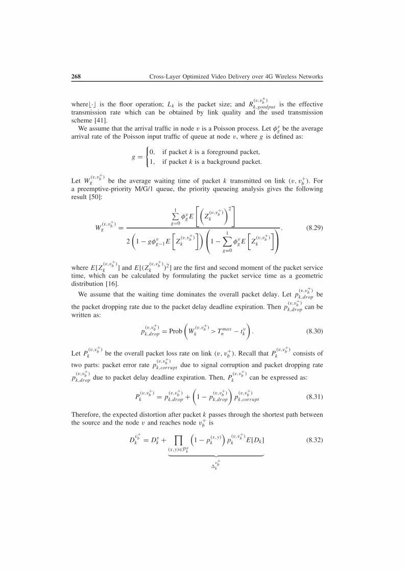
268 Cross-Layer Optimized Video Delivery over 4G Wireless Networks
where⌊·⌋ is the floor operation; Lk is the packet size; and R(v,v+
b)
k,goodput is the effective
transmission rate which can be obtained by link quality and the used transmission
scheme [41].
We assume that the arrival traffic in node v is a Poisson process. Let φvg be the average
arrival rate of the Poisson input traffic of queue at node v, where g is defined as:
g =
{0, if packet k is a foreground packet,
1, if packet k is a background packet.
Let W(v,v+
b)
g be the average waiting time of packet k transmitted on link (v, v+b ). For
a preemptive-priority M/G/1 queue, the priority queueing analysis gives the following
result [50]:
W(v,v+
b )g =
1∑g=0
φvgE
[(Z
(v,v+b
)
k
)2]
2
(1 − gφv
g−1E
[Z
(v,v+b
)
k
])1 −
1∑
g=0
φvgE
[Z
(v,v+b
)
k
]
. (8.29)
where E[Z(v,v+
b )
k ] and E[(Z(v,v+
b )
k )2] are the first and second moment of the packet service
time, which can be calculated by formulating the packet service time as a geometric
distribution [16].
We assume that the waiting time dominates the overall packet delay. Let p(v,v+
b )
k,drop be
the packet dropping rate due to the packet delay deadline expiration. Then p(v,v+
b )
k,drop can be
written as:
p(v,v+
b )
k,drop = Prob
(W
(v,v+b )
k>T max
n − tvk
). (8.30)
Let P(v,v+
b)
k be the overall packet loss rate on link (v, v+b ). Recall that P
(v,v+b
)
k consists of
two parts: packet error rate p(v,v+
b )
k,corrupt due to signal corruption and packet dropping rate
p(v,v+
b)
k,drop due to packet delay deadline expiration. Then, P(v,v+
b)
k can be expressed as:
P(v,v+
b )
k = p(v,v+
b )
k,drop +
(1 − p
(v,v+b )
k,drop
)p
(v,v+b )
k,corrupt (8.31)
Therefore, the expected distortion after packet k passes through the shortest path between
the source and the node v and reaches node v+b is
Dv+b
k = Dvk +
∏
(x,y)∈Pvk
(1 − p
(x,y)
k
)p
(v,v+b
)
k E[Dk]
︸ ︷︷ ︸�
v+b
k
(8.32)

Content-Aware Real-Time Video Streaming 269
where E[Dk] = Qk(Sk, tmaxk , p
(v,v+b
)
k , λk); and �v+b
k is the gradual distortion increase after
packet k advances from node v to node v+b .
The Integrated Proposed Routing : Recall that D(v,v+
b )
k is the distortion incurred after
packet k passes through Pvk and link (v, v+
b ) and reaches node v+b . Like Dijkstra’s short-
est path algorithm, we need to check whether D(v,v+
b )
k is less than the existing label
on node v+b . If it is, the node is relabeled by D
(v,v+b
)
k . After all the forward nodes
{v+1 , · · · , v+
b , · · · , v+B } of the working node v have been inspected and the tentative labels
[44] changed if possible, the entire graph is searched for the tentatively-labeled node with
the smallest distortion value. This node is made permanent and becomes the working
node. The distortion calculation is repeated, similar to the case of v being the working
node as shown above.
As the algorithm proceeds and different nodes become working nodes, an optimal path
will be obtained over which packet k is transmitted to the destination with the minimum
incurred distortion. Different from the fixed weight value of each hop in the classical
Dijkstra’s shortest path routing, the calculation of the weight for the current hop in the
proposed routing algorithm depends on the shortest sub-path that one packet has traversed
before the current hop.
The running time of the above routing algorithm on a graph with edges E and vertices
V can be expressed as a function of |E | and |V| using the Big-O notation. The simplest
implementation of the above algorithm stores vertices of set � in an ordinary linked list
or array, and operation Extract-Min(�) is simply a linear search through all vertices in
�. In this case, the running time is O(|V|2 + |E |) = O(|V|2).
8.6.5 Problem Solution
We observe that, for packet k in (8.27), any selected parameter CTk = {Sk,Pk} which
results in a single-packet delay being larger than T maxn cannot be chosen as part of the
optimal parameter vector CT∗k = {S∗
k ,P∗k }. Therefore, to solve (8.27), we can make use
of this fact by redefining the distortion as follows:
E[D′k] =
{∞ : E[tk] >T max
n
E[Dk] : E[tk] ≤ T maxn
(8.33)
In other words, the average distortion for a given packet with a delay larger than the
maximum permissible delay is set to infinity. This means that, given that a feasible
solution exists, the parameter vector which minimizes the average total distortion, as
defined in (8.27), will not result in any packet delay greater than T maxn . That is to say,
the minimum distortion problem, which is a constrained optimization problem, can be
relaxed into an unconstrained dual optimization problem using the redefinition above of
the single-packet delay.
Most decoder concealment strategies introduce dependencies between packets. With-
out losing the generality, we assume that owing to the concealment strategy, the current
packet will depend on its previous j packets (j ≥ 0). To solve the optimization problem,
we define a cost function Gk(CTk−j , · · · , CTk), which represents the minimum average

270 Cross-Layer Optimized Video Delivery over 4G Wireless Networks
distortion up to and including the kth packet, given that CTk−j , · · · , CTk are the decision
vectors of packets {(k − j), · · · , k} packets. For simplicity, let U := I + J be the total
packet number of the video clip. Therefore, GU (CTU−j , . . . , CTU ) represents the min-
imum total distortion for all the packets of the video clip. Clearly, to solve (8.27) is
equivalent to solving:
mininizeCTU−j ,···,CTU
GU (CTU−j , . . . , CTU ). (8.34)
The key observation for deriving an efficient algorithm is the fact that given j + 1 deci-
sion vectors CTk−j−1, · · · , CTk−1 for the (k − j − 1)st to (k − 1)st packets, and the cost
function Gk−1(CTk−j−1, · · · , CTk−1), the selection of the next decision vector CTk is
independent of the selection of the previous decision vectors CT1, CT2, · · · , CTk−j−2.
This means that the cost function can be expressed recursively as:
Gk
(CTk−j , · · · , CTk
)= minimize
CTk−j−1,···,CTk−1
{Gk−1
(CTk−j−1, · · · , CTk−1
)+ E[Dk]
}.
(8.35)The recursive representation of the cost function above makes the future step of the
optimization process independent from its past step, which is the foundation of dynamic
programming. The problem can be converted into a graph theory problem of finding the
shortest path in a directed acyclic graph (DAG) [39]. Let |S| be the number of possible
values of Sk, then computational complexity of the algorithm is O(U × |S|j+1), which
depends directly on the value of j . For most cases, j is a small number, so the algorithm is
much more efficient than an exhaustive search algorithm with exponential computational
complexity.
8.6.6 Performance Evaluation
Experiments are designed using H.264/AVC JM 12.2 for the video clip called “Mother
and Daughter”. Before video encoding, the identification of the ROI’s which commonly
emerge as moving foregrounds, is performed by six stages: a) Background Subtraction,
b) Split-and-Merge Segmentation, c) Region Growing, d) Morphological Operations, e)
Geometric Correction and f) Contour Extraction. The results of the different stages of the
operation above are shown in Figure 8.16.
Recall that the foreground packets are first scheduled when both the foreground and
background packets are present simultaneously in the queue of a node. To compare the
different quality of different received content, the peak signal-to-noise ratio (PSNR) for
the foreground (region of interest), the background and the holistic video sequence case
(corresponding to the case of no identification of regions of interest (NO-IRI)) are calcu-
lated separately. Figure 8.17 shows the PSNR performance comparison for the proposed
framework with different single-packet delay deadlines. We consider three different dead-
line values (5ms, 10ms, 15ms). The ROI has a larger comparative PSNR improvement
over NO-IRI and the background in the case of 5ms than the other two cases: 10ms and
15ms. In other words, the more stringent the single-packet delay, the more comparative
PSNR improvement of the ROI the proposed framework can offer. This shows that our

Content-Aware Real-Time Video Streaming 271
(a) (b) (c)
(d) (e) (f)
Figure 8.16 The identification of ROI’s
5 10 150
5
10
15
20
25
30
35
40
Single-packet delay budget (ms)
PS
NR
(d
B)
NO IRI
Foreground (ROI)
Background
Figure 8.17 PSNR vs. different single-packet delay deadlines/budgets
cross-layer framework is extremely applicable to the content-aware video communications
over delay-stringent or rate-limited wireless multi-hop networks.
To show the received video quality at the destination, we plot the 61th frame of the
“Mother and Daughter” sequence obtained in different scenarios. From Figure 8.18(b)
and 8.18(c), we can see that when the single-packet delay deadline becomes smaller,
the quality of ROI does not deteriorate as much as the quality of the background. From
Figure 8.18(c) and 8.18(d), we can see that with the same single-packet delay deadline,
the ROI in the cross-layer framework has a better quality than in the case of NO-IRI.

272 Cross-Layer Optimized Video Delivery over 4G Wireless Networks
(a) Theoriginal (b) Tmax
= 10ms
(c) Tmax
= 5ms (d) NO-IRIwithTmax
= 5msn n
n
Figure 8.18 Video frame quality
8.7 Cross-Layer Optimization for Video Summary Transmission
8.7.1 Background
In recent years, universal multimedia access (UMA) [51–53] has emerged as one of
the most important components for the next generation of multimedia applications. The
basic idea of UMA is universal or seamless access to multimedia content by automatic
selection or adaptation of content following user interaction. As mobile phones have
grown in popularity and capability, people have become enthusiastic about watching
multimedia content using mobile devices and personalizing the content, for example,
summarizing the video for real-time retrieval or for easy transmission. In general, the video
summarization algorithm will generate a still-image storyboard, called a video summary,
which is composed of a collection of salient images extracted from the underlying video
sequence (as shown in Figure 8.19). Therefore, video summary is a special format of
the video clip whose correlation between frames is not as high as with normal clips, but
where losing consecutive or continuous summary frames might cause severe damage to
an understanding of the summary content. The summary could be generated automatically
or selected by user’s interaction.
Although a great deal of work on video summarization can be found in the literature
[54–56], the issue of transmission of video summary has gained little attention. [57]
extends the work of [56] into the wireless video streaming domain, however packet loss
factor owing to unsatisfactory wireless channel conditions has not been considered in the
framework. In [58], packet loss is considered in video summary transmission, and the
key frames that minimize the expected end-to-end distortion are selected as the summary
frames. However, source coding has not been optimized in the optimization framework,

Cross-Layer Optimization for Video Summary Transmission 273
Figure 8.19 An example of a 10-frame video summary of the Stefan sequence
which might impact directly on the perceived quality of the results. In addition, the
algorithm does not guarantee a good content coverage of the selected frames because the
potential packet loss penalty biases heavily the selection process.
In wireless networks, packet loss is due mainly to the fading effect of time-varying
wireless channels. Adaptive modulation and coding (AMC) has been studied extensively
and advocated at the physical layer, in order to match transmission rates to time-varying
channel conditions. For example, in order to achieve high reliability at the physical layer,
one has to reduce the transmission rate using either small size constellations, or powerful
but low-rate error-correcting codes [59–61]. An alternative way to decrease packet loss
rate is to rely on the automatic repeat request (ARQ) protocol at the data link layer, which
requests retransmissions for those packets received in error. Obviously, by allowing for a
very large retransmission number, ARQ can guarantee a very low packet loss rate. How-
ever, in order to minimize delays and buffer sizes in practice, truncated ARQ protocols
have been widely adopted so as to limit the maximum number of transmissions [62].
To sum up, the link adaptation technique formed by AMC and ARQ provides greater
flexibility in delivering the summary frames.
In this section, within an quality-driven framework, we focus our study on the
cross-layer optimization of the video summary transmission over lossy networks. We
assume that a video summarization algorithm that can select frames based on some
optimality criteria is available in the system. Therefore, a cross-layer approach is
proposed optimize to jointly the AMC parameters at the physical layer, the ARQ
parameters at the data link layer and the source coding parameters at the application
layer in order to achieve the best quality of reconstructed video clips from received video
summaries. Clearly, owing to the spectacular characteristics of video summary data, the
general cross-layer optimization schemes proposed recently for normal video sequences
in [63] and [64] do not cover automatically summary data transmission. As an example,
the neighboring summary frames have typically less correlation in order to cover the
content variation of the video clip, and thus the normal temporal-based error concealment
algorithm considered in [63] and [64] would not be efficient in the current scenario.
In [65], a cross-layer multi-objective optimized scheduler for video streaming over the
1xEV-DO system is presented. With the usage of decodability and semantic importance
feedback from the application layer to the scheduler, [65] focuses on determining the best

274 Cross-Layer Optimized Video Delivery over 4G Wireless Networks
allocation of channel resources (time slots) across users. However, the joint optimization
of source coding and transmission parameters has not been considered in the framework.
Clearly, to achieve the best delivered video quality while maintaining a good content
coverage by providing tunable parameters so as to avoid consecutive summary frames
being lost simultaneously is not a trivial task. The tradeoff among the selected parameters
in these layers is mixed; for example, to maintain a reasonable delay, the source coding
might choose a coarser parameter, or AMC chooses a larger size constellation or a higher
rate FEC channel code, which will increase the vulnerability of coded frames and will
result in unacceptable video quality. However, if source and channel coding use more
bits, with the increase of packet length, the probability of packet loss increases, and ARQ
might have to increase the number of retransmission trials in order to reduce the problem
of quality owing to packet loss, which will then result in excessive delay. Therefore, the
cross-layer optimization approach is a natural solution to for improving overall system
performance.
8.7.2 Problem Formulation
We study a cross-layer framework that optimizes parameter selection in AMC at the
physical layer, ARQ at the data link layer and source coding at the application layer
in order to achieve the best quality of reconstructed video clip from the received video
summary.
The following notation will be used. Let us denote by n the number of frames of
a video clip {f0, f1, . . . , fn−1}, and m the number of frames of its video summary
{g0, g1, . . . , gm−1}. Let Si and Bi be the coding parameters and the resultant consumed
bits of the ith (i = 0, 1, . . . , m − 1) video summary frame in lossy source coding. The
summarization with different coding parameters will produce summary frames with dif-
ferent frame lengths. Large size frames will be fragmented into multiple packets for
transmission at lower layers. Let Qi denote the number of fragmented packets of the
ith summary frame. Let Ni,q and Fi,q be the number of transmissions and the packet
size for the qth packet of the ith summary frame, respectively. To improve channel uti-
lization, AMC is designed to update the transmission mode for every transmission and
retransmission of each packet. Let Ri,q,n(Ai,q,n, Ci,q,n) be the rate (bits/symbol) of AMC
mode used at the nth transmission attempt when transmitting the qth packet of the ith
summary frame, where Ai,q,n and Ci,q,n are the corresponding modulation order and cod-
ing rate. We assume that the transmission rate of the physical layer channel is fixed,
denoted by r (symbols/second). Clearly, the delay in transmitting the whole summary can
be expressed by:
T =
m−1∑
i=0
Qi∑
q=1
Ni,q∑
n=1
[Fi,q(Si , Bi)
Ri,q,n(Ai,q,n, Ci,q,n) ∗ r+ TRTT
](8.36)
where TRTT is the maximum allowed RTT to get the acknowledgement packet via the
feedback channel before a retransmission trial.
Let ρi(Si , Bi, Nmax, Ai,q,n, Ci,q,n, γi,q,n) be the loss probability of the ith summary
frame, where Nmax is the maximum transmission number for one packet and γi,q,n is the
instantaneous channel SNR. Note that any summary frame may possibly get lost during

Cross-Layer Optimization for Video Summary Transmission 275
video transmission. However, in order to simplify the problem of formulation, we assume
that the first summary frame would be guaranteed to be received. Then the expected
distortion of the video clip can be calculated by:
E[D] =
n−1∑
k=0
E[D(fk, fk)]
=
m−1∑
i=0
li+1−1∑
j=li
i∑
b=0
{(1 − ρi−b)d[fj , gi−b(Si−b)] ·
b−1∏
a=0
ρi−a
}(8.37)
where fk is the reconstructed kth frame from the received summary at the receiver side,
gk(Sk) is the reconstructed kth summary frame, li is the index of the summary frame gi
in the video clip and function d() is the distortion between two frames. We use the mean
squared error (MSE) between the two frames as the metric for calculating the distortion.
The same distortion measure for the video summary result has been used in [56–58].
The problem at hand can be formulated as:
Min E[D], s.t. : T ≤ Tmax (8.38)
where Tmax is a given delay budget for delivering the whole video clip.
In this work, we consider the content coverage issue of the received summary. In other
words, if a chunk of continuous summary frames is lost owing to channel error, then the
coverage of the received summary for the original clip would be degraded significantly.
To prevent such a problem but still keep the problem as general as possible, we define L
so that the case of L or more than L consecutive summary frames being lost will never
happen. For instance, if L = 2 then no neighboring summary frames can be lost together
during transmission. So that the distortion can be calculated by:
E[D] =
n−1∑
k=0
E[D(fk, fk)]
=
m−1∑
i=0
li+1−1∑
j=li
min(i,L−1)∑
b=0
{(1 − ρi−b)d[fj , gi−b(Si−b)] ·
b−1∏
a=0
ρi−a
}(8.39)
It is important to realize that the value of L is a constant programmable by the system,
and the introduction of L does not narrow down the original problem. As you may notice,
when we set L = m, equation (8.39) is equal to equation (8.37).
If we set L = 2 in (8.39), it is very clear that for the ith summary frame, there are
only two possibilities: either it is received or it is lost but its previous summary frame is
received. Let us denote by Gi the chance of the ith summary frame being not lost, so
Gi = 1 means it is guaranteed to be received, otherwise it is not guaranteed. Based on
the constraint, we need max(Gi, Gi−1, . . . , Gi+1−L) = 1 for all i ∈ [0,m − 1]. Gi can be
guaranteed and derived by link adaptation, which will be discussed in a later section.

276 Cross-Layer Optimized Video Delivery over 4G Wireless Networks
For delay issue, we hope that the total delay T of delivering all summary frames satisfies
T ≤ Tmax. Therefore, the problem is:
MinE[D], s.t.: T ≤ Tmax, and
max(Gi ,Gi−1, . . . ,Gi+1−L)=1, i ∈ [0,m−1] (8.40)
Once we work out problem (8.40), the optimal parameter combinations, i.e. source cod-
ing parameter Si , AMC modulation order Ai,q,n and channel coding rate Ci,q,n, and
ARQ transmission number Nmax are obtained to transmit the ith summary frame, which
minimizes the whole clip distortion and satisfies certain predefined delay constraints.
8.7.3 System Model
The system model of the cross-layer framework is shown in Figure 8.20, which consists
of a three-layer structure and a controller. At the application layer, summarization is
performed on the target video clip and large size summary frames are fragmented into
multiple packets for transmission at lower layers. At the data link layer, the ARQ protocol
is adopted. If an error is detected in a packet, a retransmission request is generated by the
receiver and is sent to the transmitter via a feedback channel. The transmitter arranges
retransmission of the requested packet. If a packet is not received correctly after Nmax
transmission attempts, we will declare packet loss, then the summary frame to which the
lost packet belongs is also regarded as lost. At the physical layer, we assume that multiple
transmission modes are available as shown in Table 8.4, with each mode consisting of
Buffer
Application LayerVideo Summarization
Application LayerVideo Reconstruction
Data Link LayerARQ
Physical LayerAMC(Mod&coding)
Rayleigh Fading Channel
Data Link LayerARQ
Physical Layer
AMC(Dmod&Decoding)
AMC Mode Selection
Retransmission Request
Si
Nmax
(Ai , Ci)
Controller
InputBuffer
Output
Link Adaptation
Channel
Estimator
Figure 8.20 The system model of cross-layer optimization for video summary transmission

Cross-Layer Optimization for Video Summary Transmission 277
Table 8.4 AMC Modes at the Physical Layer
Mode1 Mode2 Mode3 Mode4 Mode5 Mode6
Modulation BPSK QPSK QPSK 16-QAM 16-QAM 64-QAM
Coding Rate Cm 1/2 1/2 3/4 9/16 3/4 3/4
Rm (bits/sym.) 0.50 1.00 1.50 2.25 3.00 4.50
am 1.1369 0.3351 0.2197 0.2081 0.1936 0.1887
bm 7.5556 3.2543 1.5244 0.6250 0.3484 0.0871
a specific modulation and FEC code pair as in the 3GPP, HIPERLAN/2, IEEE 802.11a,
and IEEE 802.16 standards [66–68]. Based on channel state information (CSI) from the
channel estimator, the transmitter updates the AMC mode for the next packet transmission.
Coherent demodulation and maximum-likelihood (ML) decoding are used at the receiver.
The decoded bit streams are mapped to packets, which are pushed upwards to the data
link layer. If all fragmented packets of the summary frame gi are delivered correctly,
summary frame gi is saved into the buffer, and video clip frames fli through fli+1−1
are reconstructed with gi . If gi does not reach the receiver after some fixed time, the
video clip frames fli through fli+1−1 will be reconstructed with the previously received
summary frame. Obviously, the receiver only need a buffer that can contain one summary
frame, i.e. the latest received summary frame.
From description above, it is obvious that AMC combined with ARQ performs a link
adaptation in a joint approach. For a fixed video summary, say {g0, g1, . . . , gm−1}, the
link adaptation can guarantee the constraint max(Gi, Gi−1, . . . ,Gi+1−L)=1 in problem
(8.40), and produce the summary frame error rate (FER) ρi and transmission time Ti
for each summary frame gi . The detailed link adaptation and close-form expressions for
(ρi, Ti) will be clarified in section 8.7.4.
The controller is the most important part of the system, which is equipped with all
possible values of the key parameters of each layer. These parameters include the coding
parameter S at the application layer, the allowed maximum transmission number Nmax at
the data link layer, and the available AMC modes with modulation order and FEC code
rate pair (A, C). Note that here S, A, and C are parameter allocation vectors for m − 1
summary frames, for example, S = {S1, S2, . . . , Sm−1}.The following is a brief list of the performance flows of the cross-layer framework.
• When there is a video clip to transmit, based on the current average SNR γ from
the channel estimator, from all possible values of parameter set {S, Nmax, A,C}, the
controller first calculates all possible theoretical values of pair (ρi, Ti) for all possible
summary frames by using the close-form expressions of link adaptation performance
with the constraint max(Gi ,Gi−1, . . . , Gi+1−L) = 1, i ∈ [0, m − 1].
• With the total delay budget Tmax, the controller use all possible (ρi, Ti)s for the whole
summary to solve problem (8.40). The group values of {S, Nmax, A,C} corresponding
to the optimal solution of problem (8.40) are the optimal parameters to transmit the
whole video summary.
• The obtained optimal parameters {S, Nmax, A,C} are assigned to the corresponding
layers, then the whole video summary is sent out frame by frame.
• Corresponding video clip frames are reconstructed with the newly received summary
frame.

278 Cross-Layer Optimized Video Delivery over 4G Wireless Networks
We next list the operating assumptions adopted in this work.
• The channel is frequency-flat, meaning that it remains time invariant during a packet
but varies from packet to packet. Thus, AMC is adjusted on a packet-by-packet basis.
In other words, AMC scheme is updated for every transmission and retransmission
attempt. The channel quality is captured by a single parameter, namely the received
SNR γ . we adopt Rayleigh channel model to describe γ statistically. The received
SNR γ per packet is thus a random variable with a probability density function (pdf):
pγ (γ ) =1
γexp
(−
γ
γ
)(8.41)
where γ := E{γ } is the average received SNR.
• Perfect channel state information (CSI) is available at the receiver. The corresponding
mode selection is fed back to the transmitter without error and latency. This assumption
could be at least satisfied approximately by using a fast feedback channel with powerful
error control information as adopted in IEEE 802.16 [68].
• Error detection based on CRC is perfect, provided that sufficiently reliable error detec-
tion CRC codes are used.
8.7.4 Link Adaptation for Good Content Coverage
In this section, we explain how link adaptation can guarantee constraint max(Gi ,
Gi−1, . . . , Gi+1−L)=1, and derive the close-form expression of (ρi, Ti).
Actually, it is impossible to guarantee strictly constraint max(Gi, Gi−1, . . . , Gi+1−L)=1, owing to the fading characteristics of wireless channels. Let PL be the probability
that L consecutive summary frames are lost simultaneously. We assume PL to be a very
small value, say 10−2, to approximate constraint max(Gi, Gi−1, . . . ,Gi+1−L) = 1 is
satisfied. Then the goal of link adaptation becomes to guarantee PL with the least total
transmission delay.
Since the processing unit of link adaptation is packet, we need to transform PL into
target packet error rate Ptarget of lower layers. Let Ls , Lf and La be summary frame size,
fragmentation packet size and the actual packet length of link adaptation, respectively,
According to different summary frame sizes, there are two possible cases:
• The summary frame size is smaller than the fragmentation packet size. Since there is
no need to do fragmentation, we have Ptarget = PL1/L and La = Ls .
• The summary frame size is larger than the fragmentation packet size, where fragmenta-
tion is necessary. A summary frame of length Ls will be fragmented into Np =⌈Ls/Lf ⌉packets. ⌈⌉ is the smallest integer greater than or equal to a given real number. The
actual packet size La of the first ⌈Ls/Lf ⌉ − 1 packets equals to Lf , and the actual
packet size L′a of the final packet is Ls − ⌊Ls/Lf ⌋ · Lf . The target PER should be as
follows:Ptarget = 1 − (1 − PL
1/L)1/Np (8.42)
In both of the cases above, Ptarget can be regarded as the required PER at the data link
layer. Next we explain how to guarantee Ptarget with transmission packet size La by AMC

Cross-Layer Optimization for Video Summary Transmission 279
and ARQ. Let us define a PER upper bound PAMC such that the instantaneous PER is
guaranteed to be no greater than PAMC for each chosen AMC mode at the physical layer.
Then the PER at the data link layer after Nmax transmissions is no larger than PNmax
AMC . To
satisfy Ptarget, we need to impose:
PNmax
AMC = Ptarget, i.e., PAMC = P1/Nmaxtarget (8.43)
We assume each bit inside the packet has the same bit error rate (BER) and bit-errors are
uncorrelated, the PER can be related to the BER through:
PER = 1 − (1 − BER)La (8.44)
for a packet containing La bits. For any AMC mode, to guarantee the upper bound PAMC,
the required BER to achieve is:
BERAMC = 1 − (1 − PAMC)1/La (8.45)
Since exact closed-form BERs for the AMC modes in Table 1 are not available, to simplify
the AMC design, we adopt the following approximate BER expression:
BERm(γ ) = amexp(−bmγ ) (8.46)
where m is the mode index and γ is the received SNR. Parameters am and bm are
obtained by fitting (8.46) to the exact BER. To guarantee PAMC with the least delay when
transmitting a packet, we set the mode switching threshold γm for the AMC mode m to
be the minimum SNR required to achieve BERAMC. By (8.46) γm can be expressed as:
γm =1
bm
ln
(am
BERAMC
), m = 1, 2, · · · , M
γM+1 = +∞ (8.47)
where M is the total number of AMC modes available (M = 6).
Since the instantaneous PER is upper-bounded by PAMC in our AMC design, the average
PER at the physical layer will be lower than PAMC. Taking expectations over channel
realizations, the average PER at the physical layer is:
P =1
PT
M∑
m=1
∫ γm+1
γm
PERm(γ )pγ (γ )dγ
=1
PT
M∑
m=1
∫ γm+1
γm
[1 − (1 − amexp(−bmγ ))La ] · pγ (γ )dγ (8.48)
where PT =∫ +∞γ1
pγ (γ )dγ is the probability that channel has no deep fades and at least
one AMC mode can be adopted. Similarly, the average delay for one transmission attempt

280 Cross-Layer Optimized Video Delivery over 4G Wireless Networks
at the physical layer can be expressed as:
T =1
PT
M∑
m=1
∫ γm+1
γm
(La
Rm · r+ TRTT
)pγ (γ )dγ (8.49)
Then the average number of transmission attempts per packet can be found as [69]:
N = 1 + P + P2+ · · · + P
Nmax−1
=1 − P
Nmax
1 − P(8.50)
Then the actual PER at the data link layer is:
Pactual = PNmax
(8.51)
and the actual transmission delay for each packet at the data link layer is:
Tactual = T · N (8.52)
When to calculate the actual FER ρi and the actual delay Ti for transmitting the ith
summary frame, two cases should be considered as mentioned above:
• If the summary frame size Ls is smaller than the fragmentation packet size Lf , we
adopt La = Ls to compute P(La) and T (La) and we can have ρi = Pactual(La) and
Ti = Tactual(La) with [48–50].
• If the summary frame size Ls is larger than the fragmentation packet size Lf , we adopt
La =Lf and L′a =Ls − ⌊Ls/Lf ⌋ · Lf to compute Pactual(La), Tactual(La), P ′
actual(L′a)
and T ′actual(L
′a). Then we can have:
ρi = 1 − (1 − Pactual)Np−1 · (1 − P ′
actual) (8.53)
Ti = (Np − 1) · Tactual + T ′actual (8.54)
The closed-form expressions above of ρi and Ti will be used by the controller to cal-
culate all possible (ρi, Ti) to solve problem (8.40), which we will discuss in detail in
section VII-E.
8.7.5 Problem Solution
Optimal Solution: Since problem (8.40) is a constrained minimization problem, it can be
solved by Lagrangian relaxation. So the problem can be converted into:
Min{E[D] + λT }, s.t. :
max(Gi , Gi−1, . . . ,Gi+1−L) = 1, i ∈ [0, m − 1] (8.55)

Cross-Layer Optimization for Video Summary Transmission 281
The target to be minimized can be derived as the following Lagrangian cost function:
Jλ = E[D] + λT
=
m−1∑
i=0
li+1−1∑
j=li
min(i,L−1)∑
b=0
{(1 − ρi−b)d[fj , gi−b(Si−b)] ·
b−1∏
a=0
ρi−a + λTi
}(8.56)
Let us define a cost function Hi(ui) to represent the sum of distortion and
delay for up to ith summary frame, where ui represents the parameter vector
{Si, Nmax, Ai,q,n, Ci,q,n, γi,q,n}. Clearly it can be observed that:
Hi(ui) = Hi−1(ui−1) +
li+1−1∑
j=li
min(i,L−1)∑
b=0
{(1 − ρi−b)
· d[fj , gi−b(Si−b)]
b−1∏
a=0
ρi−a + λTi
}(8.57)
which means the process of choosing ui for the ith summary frame is independent of
{u0, u1, . . . , ui−2}, the parameters selected for the first i − 1 summary frames. This is the
fundamental of dynamic programming (DP). So the optimal solution can be found by a
shortest path algorithm.
As a toy example, we assume there are three summary frames {g0, g1, g2} to be sent
and assume L = 2. In addition, we suppose for each summary frame, there are k different
source coding options. Then the path graph will be like Figure 8.21. In this figure, each
node uai corresponds to a cost value H(ua
i ). The weight h(uai u
bi+1) on each branch from
node uai to ub
i+1 corresponds the incremental cost value when transmitting the (i + 1)th
summary frame with the bth source coding option. h(uai u
bi+1) can be computed by the
second term of the right hand side of (8.57).
As discussed before, the solution to problem (8.40) is to minimize the average distortion
D for a total delay budget Tmax in transmitting a whole video summary. With a path graph
H0(u10)
H0(u20)
H0(uk0)
h(u10u1
1)
h(u10u2
1)
h(u10uk
1)
h(uk0u2
1) h(u20uk
1)
h(uk0uk
1)
h(u20u1
1)
h(u11u1
2)
h(u11u2
2) h(u21u1
2)
h(u21u2
2)
h(uk1u1
2)
h(u11uk
2)
h(u20u2
1)
h(uk0u1
1)
h(uk1u2
2)h(u2
1uk2)
h(uk1uk
2)
u10
u20
uk0 uk
1
u12
u22
uk2
u21
u11
SE
0
0
0
... ... ...
Figure 8.21 Path graph of a 3-frame toy video summary transmission

282 Cross-Layer Optimized Video Delivery over 4G Wireless Networks
like above, the main function of the controller is to find the shortest path in the graph
with the forward DP. The obtained shortest path has the minimal distortion D , and at the
same time indicates the optimal choice of parameters {Si, Nmax, Ai,q,nCi,q,n} for source
coding and transmitting the ith summary frame.
For Jλ in [56], it has been shown that if there is a λ∗ such that:
{S∗, N∗max, A
∗, C∗} = arg min Jλ∗(S, Nmax, A,C) (8.58)
leads to T (S, Nmax, A,C) = Tmax, then {S∗, N∗max, A
∗, C∗} is also an optimal solution
to (8.40) [70]. It is well known that when λ sweeps from zero to infinity, the solution
to problem (8.58) traces out the convex hull of the distortion delay curve, which is a
non-increasing function. Hence λ∗ can be obtained via a fast convex recursion in λ using
the bisection algorithm.
Next we list the algorithm to find λ∗.
• Step 1: We judiciously choose two values of λ, λl and λu with λl ≤ λu which satisfy
the relation:
∑
i
T ∗i (λu) ≤ Tmax ≤
∑
i
T ∗i (λl) (8.59)
where∑
i T ∗i (λ) is the total delay corresponding to the shortest path found by forward
DP. A conservative choice for a solvable problem would be λl = 0 and λu = ∞;
• Step 2: λnext ←− λl+λu
2.
• Step 3: Perform forward DP through the path graph for λnext;�⇒ if
{∑i T ∗
i (λnext) =∑
i T ∗i (λu)
}, then stop, λ∗ = λu;
�⇒ else if(∑
i T ∗i (λnext)〉Tmax
), λl ←− λnext, Go to Step 2,
�⇒ else λu ←− λnext, Go to step 2.
Thus∑
i T ∗i (λ) is made successively closer to Tmax and finally we obtain the expected
λ∗. With λ∗, we perform DP for the last time and obtain the optimal shortest path. The
values of {Si, Nmax, Ai,q,nCi,q,n} corresponding to the shortest path are just the optimal
parameter values for source coding and transmitting the ith summary frame.
Implementation Considerations: From the analysis above, we can say that problem
(8.40) is converted into a graph theoretic problem of finding the shortest path in a
directed acyclic graph (DAG) [39]. The computational complexity of the algorithm above
is O(N × |U |L), with |U | denoting the cardinality of U , which depends on the number
of the optional values of parameters {S, Nmax, A,C}, but is still much more efficient than
the exponential computational complexity of an exhaustive search algorithm. Clearly for
cases with smaller L, the complexity is quite practical to perform the optimization. On
the other hand, for larger L, the complexity can be limited by reducing the cardinality
of U. The practical solution would be an engineering decision and trade off between the
computational capability and optimality of the solution. For a storage issue, it is important
to emphasize that the problem formulation and the proposed solution are quite generic and
flexible for devices with various storage and computational capabilities. For the transmit-
ter with a buffer size that only allows to store some portion of the video clip, the clip has

Cross-Layer Optimization for Video Summary Transmission 283
to be divided into a number of segments and problem (8.5) is solved for each segment. In
such cases, although the solution is not fully optimal for the video clip, the optimization
would still bring sufficient gains compared to those without optimization.
8.7.6 Performance Evaluation
In this section, experiments are designed using H.264/AVC JM 10.2 for the video clip
called “Glasgow”, which is a typical test clip. For comparison, we summarize the first
300 frames into 30 and 60 summary frames, respectively. The case with more summary
frames means a higher sampling rate thus less distortion. To simplify the problem, we
compress the summary by choosing different QP (quantization step size), and we consider
10 possible QPs (5, 10, 15, 20, 25, 30, 35, 40, 45, 50). According to each QP, the
frames have different rates and distortion values. The video summary is coded with
an intra-coding mode for each summary frame due to the lesser correlation between
neighboring frames. In addition, without loss of generality, we consider the case of L = 2,
in other words, we impose the constraint max(Gi, Gi−1) = 1˜(i ∈ [0,m − 1]) which needs
to be guaranteed by the link adaptation. Besides of the parameters to be optimized, we
assume a fixed channel transmission rate r = 6 ∗ 106 symbols/second and a fixed round
trip time TRTT = 100 milliseconds in our experiment.
Figure 8.22 and Figure 8.23 are comparisons between QP adaptation and No QP adap-
tation. In both figures, the average channel SNR γ is 25dB and we fix PL = 10−2 and
Nmax = 3. PL is the target probability that L = 2 consecutive frames are being lost
simultaneously, which should be small enough to approximately satisfy the constraint
max(Gi ,Gi−1) = 1. In Figure 8.22, where the total summary frame number is 30, the
2 4 6 8 10 12 14 16 18 20 226800
7000
7200
7400
7600
7800
8000
8200
Delay (second)
Dis
tort
ion
QP = 50
QP = 40
QP = 35
QP = 30
QP = 25 QP = 20
No QP adaptation, 30 frames
QP adaptation, 30 frames
Figure 8.22 Distortion vs. delay comparison between QP adaptation and no QP adaptation with
30 summary frames

284 Cross-Layer Optimized Video Delivery over 4G Wireless Networks
6 8 10 12 14 16 18 20 224600
4800
5000
5200
5400
5600
5800
6000
6200
6400
Delay (second)
Dis
tort
ion
QP=50
QP = 40
QP = 35
QP = 30
No QP adaptation, 60 frames
QP adaptation, 60 frames
Figure 8.23 Distortion vs. delay comparison between QP adaptation and no QP adaptation with
60 summary frames
square nodes show the distortion-delay pairs when the video summary is source coded
with the labeled QPs. The ‘v’ nodes refer to the distortion-delay budget pairs with QP
adaptation when delay budget is set equal to the delay time that the corresponding labeled
single QP takes to transmit the video summary. We can observe that QP adaptation, i.e.,
the cross-layer framework, has much distortion gain up to 6.2 % over fixed QP video
transmission when the delay is small. In the case of summary frame number equal to 60
as in 23, much more significant distortion gain up to 12 % can be obtained in small delay
regions.
Figure 8.24 shows the distortion vs. SNR comparisons between QP adaptation and
QP = 50 with different prescribed maximum transmission number for ARQ. Owing to
link adaptation performed by ARQ and AMC in a cross-layer fashion, both QP adaptation
and QP = 50 have a stable distortion level along all SNR values. Of course here the
delay difference of different schemes is not considered. We also notice that for either QP
adaptation or QP = 50, Nmax = 3 has better performance than Nmax = 1. This is because
the case with Nmax = 3 can achieve lower actual PER than with Nmax = 1 even though
they both aim to guarantee PL = 10−2. The same conclusion goes for Figure 8.25 where
the total summary frame number is 60.
Different distortion vs. delay budget with different PL (L = 2 in this work) is shown
in Figure 8.26. We observe that there is a large distortion-delay difference between
PL = 10−1 and PL = 10−2. Once PL achieves 10−2, there is no big distortion vs. delay
difference even though Nmax is different. However, in the two cases with different PL and
same Nmax = 3, the difference in distortion vs. delay is marginal. This is because with
larger Nmax, the actual PER is much lower than PL. From this figure, we can conclude
that the maximum transmission number impacts greatly on video transmission quality in

Cross-Layer Optimization for Video Summary Transmission 285
5 10 15 20 25 307500
7600
7700
7800
7900
8000
8100
8200
SNR (dB)
Dis
tort
ion
QP=50, Nmax = 1
QP adaptation, Nmax = 1
QP adaptation, Nmax = 3
QP=50, Nmax = 3
Figure 8.24 Distortion vs. average SNR comparison between QP adaptation and QP =50 with different Nmax for a 30-frame video summary
5 10 15 20 25 305600
5700
5800
5900
6000
6100
6200
6300
6400
6500
SNR (dB)
Dis
tort
ion
QP=50, Nmax = 1
QP adaptation, Nmax = 1
QP adaptation, Nmax = 3
QP=50, Nmax = 3
Figure 8.25 Distortion vs. average SNR comparison between QP adaptation and QP =50 with different Nmax for a 60-frame video summary

286 Cross-Layer Optimized Video Delivery over 4G Wireless Networks
4 6 8 10 12 14 16 18 206800
6850
6900
6950
7000
7050
7100
7150
7200
7250
7300
Delay Budget (second)
Dis
tort
ion
PL=10–1, Nmax=1
PL=10–2, Nmax=1
PL=10–1, Nmax=3
PL=10–2, Nmax=3
Figure 8.26 Comparisons of distortion vs. delay budget with different PL
4 6 8 10 12 14 16 18 204500
5000
5500
6000
6500
7000
7500
Delay budget (second)
Dis
tort
ion
30 frames, QP adaptation
60 frames, QP adaptation
Figure 8.27 Distortion vs. delay budget comparison with different summary frame
number

References 287
our cross-layer optimization framework. With the same delay budget, a larger allowed
maximum transmission number leads to better video transmission quality.
Figure 8.27 shows the distortion vs. delay budget in our proposed framework when
the summary frame number is 30 and 60 respectively both with γ = 25dB. With the
same delay budget, the case with 60 frames has better performance than the case with 30
frames. This is because with a higher sampling rate (that is, using 60 summary frames
instead of 30), the similarity and correlation between neighboring summary frames have
increased. Therefore, the distortion caused by losing one frame is reduced in this case
because the lost frame would be concealed by its neighboring summary frame with a
higher similarity.
8.8 Conclusions
In this chapter, we have discussed cross-layer optimized wireless multimedia communica-
tions and networking. A quality-driven cross-layer design framework has been discussed
in details. Then, based on this quality-driven framework, different design scenarios, such
as TFRC, content-aware delivery, routing and video summary, have been studied.
References
1. M. van der Schaar and S. Shankar, “Cross-layer wireless multimedia transmission: Challenges, principles,
and new paradigms,” IEEE Wireless Commun. Mag., pp. 50–58, Aug. 2005.
2. D. W. S. Ci, H. Wang, “A theoretical framework for quality-aware cross-layer optimized wireless multi-
media communications,” Advances in Multimedia, 2008.
3. M. V. K. Ramchandran, “Best wavelet packet bases in a rate-distortion sense,” IEEE Trans. Image Process.,
Vol. 20, No. 2, pp. 160–175, Apr. 1993.
4. “Generic coding of moving pictures and associated audio information- part 2: Video,” ITU-T and ISO/IEC
JTC1, ITU-T Recommendation H.262–ISO/IEC 13 818-2 (MPEG-2), 1994.
5. “Video coding for low bitrate communication version 1,” ITU-T, ITU-T Recommendation H.263, 1995.
6. “Coding of audio-visual objects part 2: Visual,” ISO/IEC JTC1, ISO/IEC 14 496-2 (MPEG-4 visual
version 1), 1999.
7. T. Wiegand, G. J. Sullivan, and A. Luthra, Draft ITU-T Recommendation H.264 and Final Draft Interna-
tional Standard 14496-10 Advanced Video Coding . Joint Video Team of ISO/IEC JTC1/SC29/WG11 and
ITU-T SG16/Q.6, Doc. JVT-G050rl, Geneva, Switzerland, May 2003.
8. T. Wiegand, H. Schwarz, A. Joch, F. Kossentini, and G. Sullivan, “Rate-constrained coder control
and comparison of video coding standards,” IEEE Trans. Circuits Syst. Video Technol., Vol. 13, No. 7,
pp. 688–703, 2003.
9. R. Hinds, “Robust mode selection for block-motion-compensated video encoding,” Ph.D. dissertation,
Massachusetts Inst. Technol, Cambridge, MA, 1999.
10. R. Zhang, S. L. Regunathan, and K. Rose, “Video Coding with Optimal Inter/Intra-Mode Switching for
Packet Loss Resilience,” IEEE J. Sel. Areas Commun., Vol. 18, No. 6, pp. 966–976, Jun. 2000.
11. Z. He, J. Cai, and C. W. Chen, “Joint source channel rate-distortion analysis for adaptive mode selection
and rate control in wireless video coding,” IEEE Trans. Circuits Syst. Video Technol., Vol. 12, No. 6,
pp. 511–523, June 2002.
12. D. Wu, T. Hou, B. Li, W. Zhu, Y.-Q. Zhang, and H. J. Chao, “An end-to-end approach for optimal
mode selection in internet video communication: Theory and application,” IEEE J. Sel. Areas Commun.,
Vol. 18, No. 6, pp. 977–995, June 2000.
13. Y. Andreopoulos, N. Mastronade, and M. van der Schaar, “Cross-layer optimized video streaming over
wireless multi-hop mesh networks,” IEEE J. Sel. Areas Commun., Vol. 24, No. 11, pp. 2104–2115,
Nov. 2006.

288 Cross-Layer Optimized Video Delivery over 4G Wireless Networks
14. S. Mao, Y. T. Hou, X. Cheng, and H. D. Sherali, “Multipath Routing for Multiple Description Video in
Wireless Ad Hoc Networks,” in Proc. IEEE INFOCOM , Miami, FL, Mar. 2005, pp. 740–750.
15. S. Kompella, S. Mao, Y. Hou, and H. Sherali, “Cross-layer optimized multipath routing for video com-
munications in wireless networks,” IEEE J. Sel. Areas Commun., Vol. 25, No. 4, pp. 831–840, May
2007.
16. H. Shiang and M. van der Schaar, “Multi-user video streaming over multi-hop wireless networks: A
distributed, cross-layer approach based on priority queuing,” IEEE J. Sel. Areas Commun., Vol. 25, No. 4,
pp. 770–785, May 2007.
17. D. Wu, S. Ci, and H. Wang, “Cross-layer optimization for video summary transmission over wireless
networks,” IEEE J. Sel. Areas Commun., Vol. 25, No. 4, pp. 841–850, May 2007.
18. P. Pahalawatta, R. Berry, T. Pappas, and A. Katsaggelos, “Content-aware resource allocation and packet
scheduling for video transmission over wireless networks,” IEEE J. Sel. Areas Commun., Vol. 25, No. 4,
pp. 749–759, May 2007.
19. T. Stockhammer, D. Kontopodis, and T. Wiegand, “Rate-distortion optimization for H.26L video coding
in packet loss environment,” in Proc. Packet Video Workshop, Pittsburgh,PA, 2002.
20. G. Cote, S. Shirani, and F. Kossentini, “Optimal mode selection and synchronization for robust video
communications over error-prone networks,” IEEE J. Sel. Areas Commun., Vol. 18, No. 6, pp. 952–965,
June 2000.
21. T. Wiegand, N. Farber, K. Stuhlmuller, and B. Girod, “Error-resilient video transmission using long-term
memory motion-compensated prediction,” IEEE J. Sel. Areas Commun., Vol. 18, No. 6, pp. 1050–1062,
June 2000.
22. C. Kim, D. Kang, and I. Kwang, “High-complexity mode decision for error prone environment,”
JVT-C101, May 2002.
23. Y. Wang, J. Ostermann, and Y. Q. Zhang, Video Processing and Communications . Prentice-Hall, Engle-
wood Cliffs, NJ, 2002.
24. S. Mao, D. Bushmitch, S. Narayanan, and S. Panwar, “Mrtp: A multiflow real-time transport protocol for
ad hoc networks,” IEEE Trans. Multimedia, Vol. 8, No. 2, pp. 356–369, Apr. 2006.
25. H. Schulzrinne, S. Casner, R. Frederick, and V. Jacobson, “Rtp: A transport protocol for realtime appli-
cations,” IETF Request For Comments 3550, Jul. 1999.
26. R. Stewart, K. Morneault, C. Sharp, H. Schwarzbauer, T. Taylor, I. Rytina, M. Kalla, L. Zhang, and
V. Paxson, “Stream control transmission protocol,” IETF RFC 2960, Oct. 2000.
27. H. Hsieh, K. Kim, Y. Zhu, and R. Sivakumar, “A receivercentric transport protocol for mobile hosts with
heterogeneous wireless interfaces,” in Proc. ACM Mobicom , San Diego, CA, Sep. 2003, pp. 1–15.
28. J. Yan, K. Katrinis, M. May, and B. Plattner, “Media- and TCP-Friendly Congestion Control for Scalable
Video Streams,” IEEE Trans. Multimedia, Vol. 8, pp. 196–206, Apr. 2006.
29. S. Floyd and K. Fall, “Promoting the use of end-to-end congestion control in the Internet,” IEEE/ACM
Trans. Networking , Vol. 7, pp. 458–472, Aug. 1999.
30. S. Floyd, M. Handley, J. Padhye, and J. Widmer, “Equation-Based Congestion Control for Unicast Appli-
cations,” Pro. ACM SIGCOMM , Aug. 2000.
31. A. Argyriou, “A Joint Performance Model of TCP and TFRC with Mobility Management Protocols,”
Wiley Wireless Communications and Mobile Computing (WCMC) Special Issue on Mobile IP , Vol. 6,
pp. 547–557, Aug. 2006.
32. M. Li, C. Lee, E. Agu, M. Claypool, and R. Kinicki, “Performance Enhancement of TFRC in Wireless
Ad Hoc Networks,” Distributed Multimedia Systems (DMS), September 2004.
33. Z. Fu, X. Meng, and S. Lu, “A Transport Protocol For Supporting Multimedia Streaming in Mobile Ad
Hoc Networks,” IEEE JSAC , December 2004.
34. K. Chen and K. Nahrstedt, “Limitations of Equation-based Congestion Control in Mobile Ad Hoc Net-
works,” Workshop on Wireless Ad Hoc Networking (WWAN), March 2004.
35. M. Handley, S. Floyd, J. Pahdye, and J. Widmer, “Tcp friendly rate control (tfrc): protocol specification,”
RFC 3448, Jan. 2003.
36. X. Zhu and B. Girod, “Media-Aware Multi-User Rate Allocation over Wireless Mesh Networks,” in IEEE
OpComm-06 , Sep. 2006, pp. 1–8.
37. , “Distributed Rate Allocation for Video Streaming over Wireless Networks with Heterogeneous Link
Speeds,” in ISMW-07 , Aug. 2007, pp. 296–301.

References 289
38. T. Wiegand, G. J. Sullivan, G. Bjontegaard, and A. Luthra, “Overview of the H.264/AVC Video Coding
Standard,” IEEE Trans. Circuits Syst. Video Technol., Vol. 13, No. 7, pp. 560–576, Jul. 2003.
39. G. M. Schuster and A. K. Katsaggelos, Rate-Distortion Based Video Compression: Optimal Video Frame
Compression and Object Boundary Encoding . Norwell, MA: Kluwer, 1997.
40. S. Adlakha, X. Zhu, B. Girod, and A. Goldsmith, “Joint Capacity, Flow and Rate Allocation for Multiuser
Video Streaming over Wireless Ad-Hoc Networks,” in IEEE ICC, Proc. Glasgow, Scotland , June 2007,
pp. 1747–1753.
41. D. Qiao, S. Choi, and K. G. Shin, “Goodput analysis and link adaptation for ieee 802.11a wireless lan,”
IEEE Trans. Mobile Comput., Vol. 1, No. 4, 2002.
42. Q. Liu, S. Zhou, and G. B. Giannakis, “Queuing with Adaptive Modulation and Coding over Wireless
Links: Cross-Layer Analysis and Design,” IEEE Trans. Wireless Commun., Vol. 4, No. 3, pp. 1142–1153,
May 2005.
43. D. Krishnaswamy, “Network-Assisted Link Adaptation with Power Control and Channel Reassignment in
Wireless Networks,” in Proc. 3G Wireless Conf., 2002, pp. 165–170.
44. A. S. Tanenbaum, Computer Networks. Upper Saddle River, NJ: Prentice Hall, 2003.
45. T. Clausen and P. Jacquet, “Optimized link state routing protocol,” IETF RFC 3626 , Oct. 2006.
46. R. Tupelly, J. Zhang, and E. Chong, “Opportunistic scheduling for streaming video in wireless networks,”
in Proc. Conference on Information Sciences and Systems, 2003.
47. G. Liebl, T. Stockhammer, C. Buchner, and A. Klein, “Radio link buffer management and scheduling for
video streaming over wireless shared channels,” in Proc. Packet Video Workshop, 2004.
48. G. Liebl, M. Kalman, and B. Girod, “Deadline-aware scheduling for wireless video streaming,” in Proc.
IEEE ICME , July 2005.
49. Stauffer, Chris, and Eric, “Learning patterns of activity using real-time tracking,” IEEE Transactions on
Pattern Analysis and Machine Intelligence, Vol. 22, No. 8, pp. 747–757, 2000.
50. D. Bertsekas and R. Gallager, Data Networks. Upper Saddle River, NJ: Prentice Hall, 1992.
51. P. V. Beek et al., “Metadata-driven multimedia access,” IEEE Signal Processing Magazine, pp. 40–52,
Mar. 2003.
52. A. Hanjalic and H. Zhang, “An integrated scheme for automatic video abstraction based on unsupervised
cluster-validity analysis,” IEEE Trans. Circuits Syst. Video Technol., Vol. 9, Dec. 1999.
53. B. L. Tseng, C. Lin, and J. R. Smith, “Using MPEG-7 and MPEG-21 for personalizing
videoMetadata-driven multimedia access,” IEEE Multimedia , Vol. 11, pp. 40–53, Jan. 2004.
54. D. DeMenthon, V. Kobla, and D. Doermann, “Video summarization by curve simplification,” in Proc.
ACM Multimedia , Jul. 1998.
55. Y. Gong and X. Liu, “Video summarization using singular value decomposition,” Computer Vision and
Pattern Recognition , Vol. 2, pp. 13–15, Jun. 2000.
56. Z. Li et al ., “Rate-distortion optimal video summary generation,” IEEE Trans. Image Process., Vol. 14,
pp. 1550–1560, Oct. 2005.
57. Z. Li, F. Zhai, and A. K. Katsaggelosothers, “Video summarization for energy efficient wireless streaming,”
in Proc. SPIE Visual Communication and Image Processing (VCIP), Beijing, China, 2005.
58. P. V. Pahalawatta et al ., “Rate-distortion optimized video summary generation and transmission over
packet lossy networks,” in Proc. SPIE Image/Video Communication and Processing (IVCP), San Jose, US,
2005.
59. D. L. Goeckel, “Adaptive coding for time-varying channels using outdated fading estimates,” IEEE Trans.
Commun., Vol. 47, pp. 844–855, Jun. 1999.
60. A. J. Goldsmith and S. G. Chua, “Adaptive coded modulation for fading channels,” IEEE Trans. Commun.,
Vol. 46, pp. 595–602, May 1998.
61. M. Alouini and A. J. Goldsmith, “Adaptive modulation over nakagami fading channels,” Kluwer J. Wireless
Communications , Vol. 13, pp. 119–143, May 2000.
62. E. Malkamaki and H. Leib, “Performance of truncated type-ii hybrid arq schemes with noisy feedback
over block fading channels,” IEEE Transactions on Communications , Vol. 48, pp. 1477–1487, Sep. 2000.
63. F. Zhai et al ., “Rate-distortion optimized hybrid error control for packetized video communications,” IEEE
Trans. Image Process., Vol. 15, pp. 40–53, Jan. 2006.

290 Cross-Layer Optimized Video Delivery over 4G Wireless Networks
64. H. Wang, F. Zhai, Y. Eisenburg, and A. K. Katsaggelosothers, “Cost-distortion optimal unequal error
protection for object-based video communications,” IEEE Trans. Circuits Syst. Video Technol., Vol. 15,
pp. 1505–1516, Dec. 2005.
65. T. Ozcelebi, F. D. Vito, M. O. Sunay, M. R. C. A. M. Tekalp, and J. D. Martin, “Cross-Layer Scheduling
with Content and Packet Priorities for Optimal Video Streaming over 1xEV-DO,” in Proc. VLBV05 ,
Sardinia, Italy, Sep. 2005, pp. 76–83.
66. (2004) 3GPP TR 25.848 V4.0.0, Physical Layer Aspects of UTRA High Speed Downlink Packet Access
(release 4).
67. A. Doufexi, S. Armour, M. Butler, A. Nix, D. Bull, J. McGeehan, and P. Karlsson, “A Comparison of
the HIPERLAN/2 and IEEE 802.11a Wireless LAN Standards,” IEEE Communication Magazine, Vol. 40,
pp. 172–180, May 2002.
68. (2002) IEEE Standard 802.16 Working Group, IEEE Standard for Local and Metropolitan Area Networks
Part 16: Air Interface for Fixed Broadband Wireless Access Systems.
69. Q. Liu, S. Zhou, and G. B. Giannakis, “Cross-layer combining of adaptive modulation and coding with
truncated arq over wireless links,” IEEE Transactions on Wireless Communications , Vol. 3, pp. 1746–1755,
Sep. 2004.
70. K. Ramchandran and M. Vetterli, “Best wavelet packet bases in a rate-distortion sense,” IEEE Transaction
on Signal Processing , Vol. 2, pp. 160–175, Apr. 1993.

9
Content-based VideoCommunications
9.1 Network-Adaptive Video Object Encoding
Network-adaptive video encoding is a robust video compression approach that designs and
optimizes the source encoder by considering transmission factors such as error control,
packetization, packet scheduling and retransmission, routing and error concealment. Error
resilience is gained by selecting optimally the encoding mode that enables the decoded
video to reach the minimum expected distortion for the available resources.
In this framework, we assume that the encoder knows the transmission channel charac-
teristics such as the bit error rate (BER) or the probability of packet loss (in packet-based
networks, the packet could be dropped or lost by bit error or excessive delay). This
can be either specified in the initial negotiations, or calculated adaptively from messages
exchanged by the transmission protocol. In a wireless channel, when transmission delay is
not a major issue, the probability of packet loss can be calculated easily from the channel
BER and the length of the packet. For ease of discussion, we assume that there is a lossy
channel in this section and in section 9.2. In this way, packets are either received error-free
or lost. The issues related to channels with BER will be addressed in section 9.3.
In order to evaluate received video quality, we assume that the transmitter knows the
background VOP on which the transmitted video object will be composed at the receiver,
which is possible if the encoder has sufficient knowledge of the application or if there is a
feedback channel from the decoder which provides to the encoder the information about
the composition order of the video objects and the success or failure of the delivering status
of the video packet. Otherwise, a default background VOP will be adopted. Therefore, the
distortion is calculated as the total intensity error of the composed frame. Owing to packet
loss in the transmission channel, the decoded video at the decoder is not deterministic,
and the distortion is a random variable. Therefore, the expected distortion is used as
our objective distortion metric. Clearly, the expected distortion for the i th slice can be
4G Wireless Video Communications Haohong Wang, Lisimachos P. Kondi, Ajay Luthra and Song Ci
© 2009 John Wiley & Sons, Ltd. ISBN: 978-0-470-77307-9

292 Content-based Video Communications
calculated by summing up the expected distortion of all the pixels in the slice:
E[Di] =iN+N−1
∑
j=iN
E[dj ] (9.1)
where E [dj ] is the expected distortion at the receiver for the j th pixel in the VOP, and N
is the total number of pixels in the slice. Let us denote by fjn the original value of pixel
j in VOP n , and fjn its reconstructed value at the decoder. By definition:
f jn = sj
n tjn + (1 − sjn)gj
n, f jn = sj
n tjn + (1 − sjn)gj
n (9.2)
and
E[dj ] = E[(f jn − f j
n )2] = (f jn )2 − 2f j
n E[f jn ] + E[(f j
n )2]
= (f jn )2 − 2f j
n E[sjn tjn ] − 2f j
n gjn + 2f j
n gjnE[sj
n] + E[(sjn tjn )2] + (gj
n)2 (9.3)
− 2gjnE[sj
n] + (gjn)2E[(sj
n)2] + 2gjnE[sj
n tjn ] − 2gjnE[(sj
n)2 tjn ]
where sjn(s
jn = 0 for transparent or 1 for opaque block; only binary shape is considered
here) and tjn are the corresponding shape and texture component of f
jn , s
jn and t
jn are the
corresponding shape and texture component of fjn , and g
jn is the background pixel value
at the same position.
The further calculation of E [dj ] in equation (9.3) is dependent on a concealment strat-
egy at the decoder. Out of a number of possible strategies, we consider the following
(an extension of ROPE [1]), which allows for the recursive calculation of E [dj ] at the
encoder. We assume that each row of macroblocks becomes a packet, and use ρi to denote
the probability of loss for the i th packet. To recover the lost shape (texture) macroblocks
in a packet, the decoder uses the shape (texture) motion vector of the neighboring mac-
roblocks above as the concealment motion vector. If the concealment motion vector is
not available, e.g., the macroblock above is also lost, then the decoder uses a zero motion
vector for concealment. In calculating E [dj ], the first and second moments of the recon-
structed shape and texture intensity value for the j th pixel are needed. In the following
paragraph, we demonstrate how the first moment can be calculated recursively in time.
The second moment is computed in a similar fashion, but omitted here, owing to lack
of space.
In object-based video, since texture and shape information can be independently
encoded in the intra and inter modes, we consider the following four cases:
E[sjn tjn ](I, I ) = (1 − ρi)s
jn tjn + ρi(1 − ρi−1)E[s
ks
n−1 tkt
n−1] + ρi−1ρiE[sj
n−1 tj
n−1] (9.4)
E[sjn tjn ](I, P ) = (1 − ρi)s
jn(ej
n + E[tmt
n−1]) + ρi(1 − ρi−1)E[sks
n−1 tkt
n−1]
+ ρi−1ρiE[sj
n−1 tj
n−1] (9.5)
E[sjn tjn ](P, I ) = (1 − ρi)E[s
ms
n−1]tjn + ρi(1 − ρi−1)E[sks
n−1 tkt
n−1] + ρi−1ρiE[sj
n−1 tj
n−1]
(9.6)

Network-Adaptive Video Object Encoding 293
E[sjn tjn ](P, P ) = (1 − ρi)(E[s
ms
n−1]ejn + E[s
ms
n−1 tmt
n−1]) + ρi(1 − ρi−1)E[sks
n−1 tkt
n−1] (9.7)
+ ρi−1ρiE[sj
n−1 tj
n−1]
where shape is intra coded in (9.4) and (9.5), and inter coded in (9.6) and (9.7); texture
is intra coded in (9.4) and (9.6), and inter coded in (9.5) and (9.7); sjn and t
jn are the
encoder reconstructed shape and texture of the j th pixel; pixel j in frame n is predicted
by pixel m in frame n−1 if the motion vector is available, otherwise predicted by pixel k
if the concealment motion vector is available. The subscript s and t of ks, kt , ms , and mt
in (9.4)–(9.7) are used to distinguish shape from texture, because the motion vector or
concealment motion vector of shape could be different from that of texture. Computing
E[sjn t
jn ] in (9.4)–(9.7) depend on the computing of E[s
jn] and E[t
jn ], which are calculated
recursively as follows:
E[sjn](I ) = (1 − ρi)s
jn + ρi(1 − ρi−1)E[sk
n−1] + ρi−1ρiE[sj
n−1] (9.8)
E[tjn ](I ) = (1 − ρi)tjn + ρi(1 − ρi−1)E[tkn−1] + ρi−1ρiE[t
j
n−1] (9.9)
E[sjn](P ) = (1 − ρi)E[sm
n−1] + ρi(1 − ρi−1)E[skn−1] + ρi−1ρiE[s
j
n−1], (9.10)
E[tjn ](P ) = (1 − ρi)(ejn + E[tmn−1]) + ρi−1ρiE[t
j
n−1] + ρi(1 − ρi−1)E[tkn−1] (9.11)
where shape and texture are intra coded in (9.8) and (9.9), and inter coded in (9.10)
and (9.11). It is not hard to understand that E[sksn tkt
n ] and E[smsn tmt
n ] in (9.4)–(9.7) can
be computed recursively in a similar manner as E[sjn t
jn ]. However, computing these
inter-pixel cross-correlation terms recursively may require computing and storing all
inter-pixel cross-correlation values for all frames in the video sequence. The amount
of this computation and storage is not feasible even for moderate size frame. It is natural
to use a model-based cross-correlation approximation method to estimate E [st] in terms
of E [s], E [t], E [s2], E [t2] and standard deviations σs and σt . The simplest idea is to
assume that s and t are uncorrelated, then E [st]= E[s]E [t]. In general, the model is quite
accurate to use and be proved with experiments.
Once the distortion estimation model is set up, the optimization problem can be repre-
sented by:
Minimize E[D], subject to R ≤ Rbudget (9.12)
which is obviously a simple instance of the expected distortion. In the equation, R is the
total bit rate, and Rbudget is the bit budget for the frame. The optimization is over the
source coding parameters and is restricted to the frame level. Clearly, the expected frame
distortion E[D] can be accumulated by the N packets within the frame, like E[D] =∑N
i=1 E[Di].
The problem can be easily solved by using Lagarangian relaxation and dynamic pro-
gramming, as discussed in section 6.2.4. Figure 9.1 shows the resulted R-D curves
of a simulation based on MPEG-4 VM 18.0, where the proposed network adaptive
approach and the non network-adaptive encoding method are compared by transmitting
video bitstreams over lossy channels with packet loss of 10 % and 20 %. Clearly, the
network-adaptive method has constant gains of around 2 dB for both channels.

294 Content-based Video Communications
0.2 0.4 0.6 0.8 1 1.2 1.4 1.6 1.8
×104
22
24
26
28
30
32
34
36
38
40
PS
NR
(dB
)
Rate
The first 30 frames (P-VOP) of the Bream sequence
Non network-adaptive (no packet loss)
Non network-adapative realization (packet loss = 0.1)
Non network-adaptive realization (packet loss = 0.2)
Network-adaptive estimation (packet loss = 0.1)Network-adaptive realization (packet loss = 0.1)
Network-adaptive estimation (packet loss = 0.2)
Network-adaptive realization (packet loss = 0.2)
Figure 9.1 Comparison of proposed approach with non-network-adaptive approach
9.2 Joint Source Coding and Unequal Error Protection
In video communications, various video packets may contribute differently to overall
video quality; unequal error protection (UEP) is a natural way of protecting transmitted
video data. The idea is to allocate more resources to the parts of the video sequence that
have a greater impact on video quality, while expending fewer resources on the parts
that are less significant. In [2], a priority encoding transmission scheme is proposed so
as to allow a user to set different priorities of error protection for different segments of
the video stream. This scheme is suitable for MPEG video, in which there is a decreas-
ing importance among I, P and B frames. In general, error protection can come from
various sources such as forward error correction, retransmission and transmission power
adaptation. In [3], a generic UEP forward error correction scheme is proposed, utilizing
the knowledge that almost all video packet formats have more important data closer to
the packet header. Thus, the algorithm requires that better protection be applied to the
data closer to the packet header. In [4], an optimal unequal error protection scheme for
layered video coding was proposed in order to provide an optimal bit allocation between
source coding and channel coding. In [5, 6], the trade off between transmission energy
consumption and video quality for wireless video communications is studied, where the
goal is to minimize the energy needed to transmit a video sequence with an accept-
able level of video quality and tolerable delay. By assuming that the transmitter knows
the relationship between the transmission power and the probability of the packet loss,
transmission power can be adjusted dynamically so as to control the level of protection

Joint Source Coding and Unequal Error Protection 295
provided for each packet [5, 6]. Similarly, in [7] and [8], the cost-distortion problem in
a DiffServ network is studied, by assigning unequal protection (prices) to the different
packets.
In object-based coding, video data is composed of shape and texture information, which
have completely different stochastic characteristics and bit rate proportions. For example,
in moderate or high bit rate applications, the shape data generally only occupies 0.5–20 %
of the total bit rate [9], but can have a stronger impact on reconstructed video quality
than texture. The unbalanced contribution of shape and texture information makes UEP
a natural solution to protect this type of video sequence in lossy networks. In [3, 10, 11]
and [12], UEP schemes have been explored and applied to the transmission of MPEG-4
compressed video bitstreams over error-prone wireless channels. In their work, the video
is compressed using a standard block-based approach with rectangular shape, i.e., there is
no shape information contained in the bitstream. Thus, the resulting bitstream is divided
into partitions labeled header, motion and texture, which are assumed to have a decreas-
ing order of importance. Therefore, the header and motion bits receive higher levels of
protection and the texture bits receive the lowest level of protection. In [10], I-frame
data is treated as having the same level of importance as header and motion data. In [3],
I-frame DCT data is subdivided into DC coefficients and AC coefficients, where DC is
considered to have a higher subjective importance than AC. In [10, 11] and [12], UEP
is implemented using different channel coding rates, while in [12], it is implemented by
separating the partitions into various streams and transmitting those streams over different
carrier channels meeting different QoS levels. It is reported in [3, 10, 11] and [12] that the
adoption of UEP results in a better performance than equal error protection (EEP) meth-
ods. However, this work has not considered video with arbitrarily shaped video objects.
Furthermore, it is based on pre-encoded video. Thus it does not consider optimal source
coding, nor does it incorporate the error concealment strategy used at the decoder in the
UEP framework.
Recently, a rate-distortion optimal source-coding scheme was proposed for solving the
bit allocation problem in object-based video coding [13]. There, the experimental results
indicate that for some applications shape may have a stronger impact on reconstructed
video quality than texture. This result motivates the unequal protection of the shape
and texture components of the video objects in video transmission. In this section, a
general cost-distortion optimal unequal error protection scheme for object-based video
communications is demonstrated where source coding, packet classification and error
concealment are considered jointly within the framework of cost-distortion optimization.
The scheme is applicable for packet lossy networks, that is, there is an assumption that
the packets are either received error-free or lost.
9.2.1 Problem Formulation
The problem at hand is to choose coding parameters for the shape and texture of a VOP,
so as to minimize the total expected distortion, given a cost constraint and a transmis-
sion delay constraint in a lossy network environment. This objective can also be repre-
sented by:
Minimize E[Dtot], Subject to Ctot ≤ Cmax and Ttot ≤ Tmax (9.13)

296 Content-based Video Communications
where E[Dtot] is the expected total distortion for the frame, Ctot is the total cost for a
frame, Ttot is the total transmission delay for the frame, Cmax is the maximum allowable
cost for the frame and Tmax is the maximum amount of time which can be used to transmit
the entire frame. We assume that there exists a higher-level controller which assigns a
bit budget and a cost budget to each frame in order to meet any of the delay constraints
imposed by the application. Therefore, the value of Cmax and Tmax can vary from frame
to frame, but are known constants in (9.13).
9.2.1.1 System Model
We consider an MPEG-4 compliant object-based video application, where the video is
encoded using different algorithms for shape and texture. As mentioned in [9], compared
to texture data, shape data requires relatively fewer bits to encode but has a very strong
impact on video quality. Therefore, it is natural to imagine that the unequal error pro-
tection scheme for shape and texture may provide improved performance over an equal
error protection scheme. However, implementing an unequal error protection scheme is not
straightforward because in the MPEG-4 video packet syntax, the shape and texture data are
placed in the same packet (using a combined packetization scheme). If data partitioning
is enabled, a motion marker is placed between the shape and texture data for resynchro-
nization. One way to enable unequal error protection is to use a separated packetization
scheme, where shape and texture are packed into separate packets. In a similar way as
is proposed in [10] and [11], we insert an adaptation layer between the MPEG-4 video
application and the network, which can reorganize the MPEG-4 compressed bitstream into
corresponding shape packets and texture packets. In addition, the adaptation layer can add
some forward error protection optimally to those packets. Figure 9.2 depicts the architec-
ture of the proposed video transmission system. For a wireless network using an H.223
Object-basedVideo Encoder
Packet Partition Channel Encoder
MUX
H.223/RTP Terminal
Adaptation layerMultiplex layer
Channel
Object-basedVideo Decoder
Packet merging Channel Decoder
DEMUX
H.223/RTP Terminal
Adaptation layerMultiplex layer
Figure 9.2 System block diagram

Joint Source Coding and Unequal Error Protection 297
MUX [11], we simply replace the standard adaptation layer in the H.223 multiplexing
protocol with our new layer. At the receiver side, the adaptation layer merges the shape
and texture packets and makes the output bitstream compatible with the MPEG-4 syntax.
In the following text, the separated packetization scheme is used as the default packe-
tization scheme. The coded video frame is divided into 16 × 16 macroblocks, which are
numbered in scan line order and divided into groups called slices. For each slice, there
is a shape packet and a corresponding texture packet. Let I be the number of slices in
the given frame and i the slice index. For each macroblock, both coding parameters for
shape and texture are specified. We use µSiand µTi
, respectively, to denote the coding
parameters for all macroblocks in the i th shape and texture packets, and use BSi(µSi
) and
BTi(µTi
), respectively, to denote the corresponding encoding bit rates of these packets. It
is important to point out that each packet is decodable independently in our system; that
is, each packet has enough information for decoding and is independent of other packets
in the same frame. This guarantees that a lost packet will not affect the decoding of other
packets in the same frame. Of course, errors may propagate from one frame to the next
owing to motion compensation.
9.2.1.2 Channel Model
In addition to the source coding parameters, we assume that the transmission parameters
may also be adapted per packet. By adapting the transmission parameters, we can control
the effective channel characteristics, such as the probability of loss. Another way to
view this is that each encoded packet can be sent over a set of possible transmission
channels. Each transmission channel is classified using a set of parameters, e.g., the
probability of packet loss and transmission rate. Let us denote by πSiand πTi
, the selected
service classes for the i th shape and texture packet, respectively. Similarly, let ρ(πSi)
and ρ(πTi) denote the corresponding probability of packet loss, and R(πSi
) and R(πTi)
the corresponding transmission rate. Then the total transmission time per fame is repre-
sented by:
Ttot =I
∑
i=1
[
BSi(µSi
)
R(πSi)
+BTi
(µTi)
R(πTi)
]
(9.14)
Let C(πSi) and C(πTi
) denote respectively the transmission cost per bit for the i th shape
and texture packets. The total cost used to transmit all the packets in a frame is therefore:
Ctot =I
∑
i=1
[BSi(µSi
)C(πSi) + BTi
(µTi)C(πTi
)] (9.15)
In a DiffServ network, the cost represents the price for each QoS channel, e.g., cents per
Kbyte. We assume that the service level can be pre-specified in the service level agreement
(SLA) between the Internet service provider (ISP) and the users [14]. Typically a set of
parameters is used to describe the state of each service class, including the transmission
rate bound and probability of packet loss. In this setting, a cost is associated with each

298 Content-based Video Communications
service class as specified in the SLA. By adjusting the prices for each service class, the
network can influence the class a user selects. The sender classifies each packet according
to its importance in order to better utilize the available network resources.
In a wireless network, the cost we consider in this work is represented by energy per
bit, i.e.:
C(πSi) =
P(πSi)
R(πSi), and C(πTi
) =P(πTi
)
R(πTi)
(9.16)
where P(πSi) and P(πTi
) are the corresponding transmission power for the i th shape and
texture packet, respectively. The exact relationship between transmission power, trans-
mission rate and the probability of packet loss varies for different channel models.
9.2.1.3 Expected Distortion
We assume that the transmitter only knows the probability with which a packet has
arrived at the receiver. Thus, the distortion at the receiver is a random variable. Let
E [Di] represent the expected distortion at the receiver for the i th slice. In this case:
E[Di] = [1 − ρ(πSi)][1 − ρ(πTi
)]E[DR,i] + [1 − ρ(πSi)]ρ(πTi
)E[DLT,i]
+ ρ(πSi)[1 − ρ(πTi
)]E[DLS,i] + ρ(πSi)ρ(πTi
)E[DL,i] (9.17)
where E [DR,i] is the expected distortion for the i th slice if both the shape and texture
packets are received correctly at the decoder, E [DLT,i] is the expected distortion if the
texture packet is lost, E [DLS,i] is the expected distortion if the shape packet is lost and
E [DL,i] is the expected distortion if both the shape and texture packets are lost. Clearly,
E [DR,i] depends only on the source coding parameters for the i th packet, while E [DLT,i],
E [DLS,i] and E [DL,i] depend on the concealment strategy used at the decoder.
Note that the problem formulation and solution approach presented in this chapter are
general. Therefore, the techniques developed here are applicable to various concealment
strategies used by the decoder. The only assumption we make is that the concealment
strategy is also known at the encoder. A common concealment strategy is to conceal
the missing macroblock by using the motion information of its neighboring macroblocks.
When the neighboring macroblock information is not available, the lost macroblock is
typically replaced with the macroblock from the previous frame at the same location.
It is also important to note that the formulation presented here is applicable to various
distortion metrics. In our experimental results we use the expected mean squared error
(MSE), as is commonly done in the literature [1, 5, 6, 8].
9.2.1.4 Optimization Formulation
The optimization problem (9.13) can be rewritten as:
Minimize{µSi
,µTi,πSi
,πTi}E[Dtot]

Joint Source Coding and Unequal Error Protection 299
subject to :
I∑
i=1
[BSi(µSi
)C(πSi) + BTi
(µTi)C(πTi
)] ≤ Cmax (9.18)
and
I∑
i=1
[
BSi(µSi
)
R(πSi)
+BTi
(µTi)
R(πTi)
]
≤ Tmax
We assume that the processing and propagation delays are constant and can therefore
be ignored in this formulation. The only delay we are concerned with is the transmi-
ssion delay.
9.2.2 Solution and Implementation Details
9.2.2.1 Packetization and Error Concealment
The packetization scheme, i.e., the number of macroblocks per packet, is not standardized
within the MPEG-4 standard. Some applications pack each macroblock into a packet. This
approach provides significant error resilience and encoding flexibility, but suffers from
the large transmission overhead required for each packet header. In addition, since each
packet must be decodable independently, this approach does not benefit from differential
encoding between macroblocks. In other applications, each frame is packed into a separate
packet. In this case, the transmission overhead is very small, but the resilience to channel
errors is poor, e.g., an uncorrectable local error may cause the entire frame to be discarded.
In order to balance error resilience and coding efficiency, we consider packing each
row of macroblocks into a packet. In our simulations, we consider both the combined
packetization scheme and the separated packetization scheme. It is important to note that
four extra bits per MB, indicating the 8 × 8 shape block transparency, must be added to
the texture packets in the separated packetization scheme, in order to make each packet
decodable independently.
The error concealment strategy in the simulations is identical for both shape
and texture packets. To recover the lost shape (texture) information, the decoder
uses the shape (texture) motion vector of the neighboring macroblock above as the
concealment motion vector. If the concealment motion vector is not available, e.g.,
because the above macroblock is also lost, then the decoder uses zero motion vector
concealment.
9.2.2.2 Expected Distortion
For separated packetization, since the shape data and texture data are transmitted and
decoded independently:
E[sjn tjn ] = E[sj
n]E[tjn ], and E[sjn tjn ] = E[sj
n]E[tjn ] (9.19)
This observation enables us to calculate the expected distortion efficiently (9.3) by calcu-
lating recursively the necessary moments for shape and texture independently.

300 Content-based Video Communications
9.2.2.3 Optimal Solution
In this section, we present an optimal solution for problem (9.18). We use the Lagrange
multiplier method in order to relax the cost and delay constraints. The relaxed problem
can then be solved using a shortest path algorithm.
The Lagrangian relaxation method leads to a convex hull approximation for the con-
strained problem (9.18). Let U be the set of all possible decision vectors ui for the i th
slice (i = 1, 2, . . . , I ), where ui = (µSi, µTi
, πSi, πTi
). We first define a Lagrangian cost
function:
Jλ1,λ2(u) = E[Dtot] + λ1Ctot + λ2Ttot (9.20)
=I
∑
i=1
{
E[Di] + λ1[BSi(µSi
)C(πSi) + BTi
(µTi)C(πTi
)]
+ λ2
[
BSi(µSi
)
R(πSi)
+BTi
(µTi)
R(πTi)
]}
where λ1 and λ2 are the Lagrange multipliers. It can easily be derived from [15] and
[16] that if there exists a pair λ∗1 and λ∗
2 such that u∗ = arg[minuJλ∗1,λ∗
2(u)], which leads
to Ctot = Cmax and Ttot = Tmax, then u∗ is also an optimal solution to (9.18). Therefore,
the task of solving (9.18) is converted into an easier one, which is to find the optimal
solution to the unconstrained problem:
min
I∑
i=1
{
E[Di] + λ1[BSi(µSi
)C(πSi) + BTi
(µTi)C(πTi
)] + λ2
[
BSi(µSi
)
R(πSi)
+BTi
(µTi)
R(πTi)
]}
(9.21)
Most decoder concealment strategies introduce dependencies between slices. For
example, if the concealment algorithm uses the motion vector of the macroblock above to
conceal the lost macroblock, then it would cause the calculation of the expected distortion
of the current slice to depend on its previous slice. Without loss of the generality,
we assume that the concealment strategy will cause the current slice to depend on its
previous a slices (a ≥ 0). To implement the algorithm for solving optimization problem
(9.18), we define a cost function Gk(uk−a, . . . , uk), which represents the minimum total
cost, delay and distortion up to and including the k th slice, given that uk−a, . . . , uk are
decision vectors for the (k − a)th to k th slices. Therefore, GI (uI−a, . . . , uI ) represents
the minimum total cost, delay and distortion for all the slices of the frame, and thus:
minu
Jλ1,λ2(u) = min
uI−a ,...,uI
GI (uI−a, . . . , uI ) (9.22)
The key observation for deriving an efficient algorithm is the fact that given a+1 deci-
sion vectors uk−a−1, . . . , uk−1 for the (k − a−1)th to (k−1)th slices, and the cost function
Gk−1(uk−a−1, . . . , uk−1), the selection of the next decision vector uk is independent of

Joint Source Coding and Unequal Error Protection 301
the selection of the previous decision vectors u1, u2, . . . , uk−a−2. This is true since the
cost function can be expressed recursively as:
Gk(uk−a, . . . , uk) = minuk−a−1,...,uk−1
{
Gk−1(uk−a−1, . . . , uk−1) + E[Dk]
+ λ1 · [BSk(µSk
)C(πSk) + BTk
(µTk)C(πTk
)]
+ λ2
[
BSk(µSk
)
R(πSk)
+BTk
(µTk)
R(πTk)
]}
(9.23)
The recursive representation of the cost function above makes the future step of the
optimization process independent from its past step, which is the foundation of dynamic
programming.
The problem can be converted into a graph theory problem of finding the shortest path
in a directed acyclic graph (DAG) [16]. The computational complexity of the algorithm
is O(I × |U |a+1) (|U | is the cardinality of U ), which depends directly on the value of
a . For most cases, a is a small number, so the algorithm is much more efficient than an
exhaustive search algorithm which has exponential computational complexity.
9.2.3 Application on Energy-Efficient Wireless Network
In this section, we consider an application of video transmission over a narrow-band
block-fading wireless channel with additive white Gaussian noise. The main objective
is to compare three error protection schemes: 1) UEP-UST, an unequal error protection
scheme using the separated packetization scheme, where the shape and texture data are
placed in separate packets and therefore can be transmitted over different service channels;
2) UEP-EST, an unequal error protection scheme using combined packetization (i.e., the
shape and texture are placed in the same packet) where the packets can be transmitted
over different service channels; 3) EEP, an equal error protection scheme using combined
packetization, where all the packets are transmitted over the same service channel.
9.2.3.1 Channel Model
In our simulation for video transmission over wireless channels, we assume that each
packet is sent over a narrow-band block-fading channel with additive white Gaussian
noise. We further assume the channel fading for each packet is independent, and can be
modeled by a random variable H . Thus the received signal y(t) can be represented by:
y(t) =√
H x(t) + n(t) (9.24)
where x(t) is the transmitted signal, and n(t) is an additive white Gaussian noise process
with power spectral density N0. We assume that H stays fixed during the transmission
of a packet, and varies randomly between packets. Each realization h of H is chosen
according to the a priori distribution fH (h | θ), where θ is the channel state information
(CSI) parameters known by the transmitter. Here we assume√
H is Rayleigh distributed,

302 Content-based Video Communications
and assume θ = E[H ], thus:
fH (h | θ) = 1
θe−h/θ , h ≥ 0 (9.25)
In our implementation, we assume that a packet is dropped if the capacity of the channel
realization during that block is less than or equal to the information rate. For the i th shape
packet, the capacity of the channel over which this packet is sent is:
δ(πSi) = 1
Wlog2
(
1 + hSiP(πSi)
N0W
)
(9.26)
where W is the channel bandwidth. Therefore, the probability of loss for the i th shape
packet is:
ρ(πSi) = Pr{R(πSi
) ≥ δ(πSi)} = Pr
{
R(πSi) ≥ 1
Wlog2
(
1 +hSi
P(πSi)
N0W
)}
(9.27)
= Pr
{
hSi≤ N0W
P(πSi)(2R(πSi
)/W − 1)
}
= 1 − e−N0W(2
R(πSi)/W −1)
θ ·P (πSi)
Inversely, the power can be represented by:
P(πSi) = −N0W · (2R(πSi
)/W − 1)
θ · ln ρ(πSi)
(9.28)
Similar results can be derived for the i th texture packet, and the i th packet in the combined
packetization.
9.2.3.2 Experimental Results
We encode the QCIF ‘Children’ sequence at 10fps, and setN0W
θ= 6W,W = 5MHz, and
R = 200 kbits/s. We use six classes of service channels with powers equal to 1, 2, 3, 4,
6, and 10 Watts.
We compare the UEP-UST and UEP-EST schemes with an optimal EEP reference
system. Figure 9.3 shows the cost-distortion (C-D) curves for these settings. Each point
on the C-D curve of the optimal EEP system is obtained by trying all the fixed power
levels and choosing the one that achieves the best quality for each cost constraint. The
results in the figure indicate that adapting jointly the source coding parameters along with
the selection of the transmission channel can provide significant gains in expected PSNR
over equal error protection methods. Typically, in the UEP approaches, those packets
vulnerable to packet loss (hard to be recovered by the concealment strategy employed)
but robust to compression (acceptable distortion from quantization or other approximation
processing) are sent through the better-protected channel. That is, a higher compression
ratio might be used in the higher-cost channels than the lower-cost channels in order to

Joint Source Coding and Unequal Error Protection 303
0 100 200 300 400 500 600 700 80028
29
30
31
32
33
34
35
36
37
38P
SN
R (
dB
)
Cost
The first 50 frames (P-VOP) of the Children sequence
UEP-UST
UEP-EST
EEP
Figure 9.3 Comparison of Cost-Distortion curves for the UEP-UST, UEP-EST, and EEP schemes
distribute the total cost among the various packets efficiently. Furthermore, the UEP-EST
approach outperforms the UEP-EST scheme because the UEP-EST approach has increased
flexibility in providing unequal protection for shape and texture packets.
Figure 9.4 shows the distribution of the shape and texture packets among the six
transmission channels for the UEP-UST approach when the cost constraint Cmax equals
100, 200, 300 and 800. The results indicate that the shape packets are better protected than
texture packets. During the increasing of Cmax from 100 to 300, shape packets are selected
more frequently than texture packets for transmission through the higher-cost channels.
This is because shape packets have a lower bit consumption but a strong impact on the
video quality. As shown in Figure 6.4, when Cmax = 300 at least 80 % of shape packets
are transmitted over the most expensive channel, while over 60 % of texture packets
are transmitted over the two least expensive channels. In other words, the optimization
process chooses to allocate more protection to the shape, because it impacts the end-to-end
distortion more than the texture.
9.2.4 Application on Differentiated Services Networks
In this section, we consider video transmission over a differentiated services network. We
simulate a simplified DiffServ network as an independent time-invariant packet erasure
channel. Packet loss in the network is modeled as a Bernoulli random process. In addition,
a packet is considered lost if it does not arrive at the decoder on time.

304 Content-based Video Communications
1 2 3 4 5 60
100
200
300
400N
um
ber
of packets
Channel class (Cmax = 100)
Shape packets
Texture packets
1 2 3 4 5 60
50
100
150
200
250
Num
ber
of packets
Channel class (Cmax = 200)
Shape packets
Texture packets
1 2 3 4 5 60
100
200
300
400
Num
ber
of packets
Channel class (Cmax = 300)
Shape packets
Texture packets
1 2 3 4 5 60
100
200
300
400
Num
ber
of packets
Channel class (Cmax = 800)
Shape packets
Texture packets
Figure 9.4 Distribution of shape and texture packets in the UEP-UST system

Joint Source-Channel Coding with Utilization of Data Hiding 305
Table 9.1 Parameters of four service classes
Class 1 2 3 4
Probability of packet loss 0.2 0.1 0.05 0.01
Transmission rate (Kbps) 315 420 525 630
Cost (microcents/Kilobits) 10 30 60 100
100 200 300 400 500 600 700 80026
27
28
29
30
31
32
33
34
PS
NR
(d
B)
Cost
The first 30 frames (P-VOP) of the Bream sequence
UEP-UST
UEP-EST
EEP
Figure 9.5 Comparison of UEP-UST with UEP-EST and EEP
There are four QoS channels available, whose parameters are defined in Table 9.1. The
costs for each class is set proportionally to the average throughput of the class, which
takes into account the transmission rate and probability of packet loss. In this experiment,
a compressed RTP header (5 Bytes) has been added to each packet [17].
We encode the QCIF ‘Bream’ sequence at 30 fps and transmitted it over the simulated
DiffServ network. Figure 9.5 shows the C-D curves for all the schemes. As expected,
UEP-UST outperforms UEP-EST and both approaches outperform the EEP system.
9.3 Joint Source-Channel Coding with Utilization of Data Hiding
Data hiding [18] has been widely used in many applications. In copyright protection
applications [19–21], specific signature information, called the watermark, is hidden

306 Content-based Video Communications
invisibly inside a host image or video data source, by the owners before distributing their
products. Later, the owner can retrieve the hidden signature from a distributed image
or video product in order to prove its authenticity. In secure transmission applications
[22], the secure data (for example, control information) are embedded inside the regular
data to be transmitted in a standardized and open form, or over an insecure or readily
available medium, such as the Internet, allowing only those authorized at the receiver
side to retrieve the additional hidden informtion. An outstanding feature of data hiding
scheme is that it provides the opportunity of retrival of hidden information even without
the availability of the original host.
Using data hiding in error resilient video encoding and decoding has attracted much
attention recently, for example, it can be used for increasing the error detection rate in
video communication applications [23]. It has been proven that embedding redundant
information, such as edge information and motion vectors, in encoding is very helpful for
future error concealment. In [24] redundant information was embedded into the motion
vectors of the next frame for protecting the motion vectors and coding modes of the
current frame. Although this data embedded coding scheme degenerated the coding per-
formance of half-pixel motion compensation back to integer-pixel motion compensation,
the embedded information can effectively help the decoder to recover the motion vec-
tors of the corrupted GOB (group of block) and conceal the missing blocks. The limited
embedding capacity restricted the effectiveness of the proposed approach to cases of at
most one corrupted GOB in each frame. In [25] the block type and major edge direction
of content blocks of an image was embedded into the DCT coefficients of another block.
In [26] and [3] one or several copies of an approximation version of the original frame
was embedded inside the frequency coefficients. In [27] the FEC coded parity bits of
the upper layer (the most important layer) were embedded in the least significant layer
of a JPEG2000 code stream. In [28] the DCT coefficients of the segmented audio signal
and the coarsest resolution chrominance components of the video frames were embedded
in the luminance components. In [29], the data embedding scheme was used for error
concealment for H.264 video encoding and transmission, where the edge information is
embedded in I-frames, and the motion information, the reference frame, the code modes
and the error concealment scheme are embedded in P-frames.
The general data hiding scheme is shown in Figure 9.6. At the sender side, a message
m, encrypted optionally using a key K, is embedded in the host signal sequence x to
form a signal sequence y, which is transmitted over a noisy channel. Signal y could be
corrupted and become y at the receiver. The decoder extracts the estimated embedded
signal m. This process may require signal x, and key K. In error recovery and similar
applications, we should note that a) key K may not be necessary, b) m can be correlated
Embedding Extraction
ˆ ˆ
ˆ
yyx
m
x
m
NoiseSender Receiverk k
Figure 9.6 General data hiding scheme

Joint Source-Channel Coding with Utilization of Data Hiding 307
to, or a subset of x, and c) at the receiver side the signal x is reconstructed from signals
y and m.
There are two popular data embedding and extracting approaches, the spread spectrum
method [19, 30] and the odd-even method [31]. We describe both methods in the following,
and for simplicity, we assume that the host data x is the DCT coefficients of the frame.
In the spread spectrum method, the data to be embedded is spread over the host data
so that the embedded energy for each host frequency bin is negligible, which makes the
embedded data imperceptible. First, an algorithm is used to generate a pseudo-noise signal
sequence w , which has values in the range of [−1,1] and is of zero mean. Then each
embedding signal mi is spread into M different locations {i, 2i, 3i, . . . ,Mi} inside the
host sequence as:
mj
i = miwi×j , (j = 1, 2, . . . ,M) (9.29)
The embedding process is:
yi×j = xi×j + αmj
i (9.30)
where α is a scaling factor that determines the strength of the embedded information, that
is, as α increases, the embedded data becomes more robust, but the difference between
x and y increases. At the receiver side, the seed for generating the random sequence is
known and thus w can be generated. Then an estimation of the spread version of the
embedded signal is performed as follows:
mi = 1
M
M∑
j=1
yi×jwi×j (9.31)
In the odd-even embedding method, the data is embedded in the non-zero quantized
AC coefficients. If the bit to be embedded is ‘0’, the AC coefficient will be forced to be
an even number, otherwise, the AC coefficient will be forced to be an odd number. The
scheme can be represented by:
Embed(p, b) =
p + 1 if p > 0 and (p − b) mod 2 �= 0
p − 1 if p < 0 and (p − b) mod 2 �= 0
p otherwise
(9.32)
where p is the AC coefficient and b is the embedded bit.
The data extraction is quite straightforward, and can be represented by:
Extract(p′) = p′ mod 2 (9.33)
where p′ represents a received AC coefficient.
Clearly, in both methods, x = x cannot be guaranteed. However, if we assume that the
embedded bitstream is either lost (dropped because of excessive delay or an uncorrectable
bit error is detected) or received correctly (y = y), then for the received bitstream, the
odd-even embedding method guarantees that m = m. This cannot be guaranteed by the
spread spectrum method.

308 Content-based Video Communications
9.3.1 Hiding Shape in Texture
In MPEG-4, the data partitioned packetization scheme is applied so as to increase the error
resilience. In this scheme, the shape and texture data are packed in the same packet (see
Figure 9.7) but separated by a motion marker. In this way, when the partition containing
texture data is corrupted, but shape and motion data are received, the obtained motion
vector can be used to conceal the corrupted texture. However, since the decoding of the
texture partition relies on information stored in the shape partition, such as texture motion
vector, texture coding mode and shape BAB type, the entire packet will be discarded when
the shape data is corrupted, even if the texture data is uncorrupted.
We consider the embedding of information of shape and motion partition into the texture
data in order to make it self-decodable. Thus, texture data can be used even if the shape
partition is corrupted. In addition, the embedded shape and motion data could also help
to partially recover the lost shape and motion paritition. As shown in Table 9.1, the four
types of data, shape BAB type, COD, texture coding mode and CBPC, are critical for
the decoding of texture. We could embed the integer motion vectors in the range [−16,
16], and also a lossy version of the shape (using a lower-resolution of a 4 × 4 bitmap to
represent the original 16 × 16 BAB).
It is very important to decide the amount of embedded information, because
over-embedding could bring intolerable texture distortion, and the number of DCT
coefficients limits the embedding capacity. Here, the odd-even method is used, which
can guarantee the correct extraction of the embedded information. Then, the embedding
capacity is further reduced to the number of non-zero DCT coefficients. To allocate the
embedded data within limited spots efficiently, we propose five levels of embedding
modes, that is, 0) No embedding; 1) Embed critical information (these data necessary for
texture decoding as shown in Table 9.2) only; 2) Embed critical information, and motion
vectors; 3) Embed critical information and lossy shape; 4) Embed critical information,
motion vector and lossy shape. The embedding mode itself is also embedded inside the
texture data.
The advantage of the scheme of ‘hiding shape in texture’ is demonstrated with a simple
example shown in Figures 9.8 and 9.9. We encode the ‘Children sequence’ and transmit it
over a noisy wireless channel. During transmission, the shape partition of the 3rd packet
(3rd row of macroblocks) of the 16th frame (as shown in Figure 9.8(b)) is corrupted;
thus the whole packet is discarded and a common concealment strategy, which uses the
motion vectors of above macroblocks to get predictive data from the previous frame (as
shown in Figure 9.8(a)), is called to recover the lost packet (as shown in Figure 9.8(c)). In
Figure 9.9, the proposed data embedding scheme is used when the embedding level equals
Bab_type CR ST BAC COD MCBPC
AC_pred_flag CBPYMotion Marker DC data AC data
MVDs MV MVD2-4
Figure 9.7 MPEG-4 Data partitioned motion shape texture syntax for P-VOPs

Joint Source-Channel Coding with Utilization of Data Hiding 309
Table 9.2 Information to be embedded into texture data
Bits embedded Necessary for texture decoding
Transparent: 1
Shape BAB type Opaque: 2 Y
Boundary: 2+4
COD 1 Y
Texture mode 1 Y
CBPC 2 Y
Texture Motion vector 10 N
Lossy shape 4–16 N
(a) PSNR = 39.91dB (b) PSNR = 37.31dB, Rate = 5758 (c) PSNR = 23.08dB
Figure 9.8 Example of reconstructed frame of ‘Children’ sequence: a corresponds to the 15th
frame, b and c correspond to the 16th frame; in c, the shape partition of the 3rd packet is corrupted
and then concealed
2, 3 and 4, respectively. Clearly, the embedding of shape and motion information increases
the bit rate slightly and causes a very slight reduction in texture quality. However, the
embedded information is very helpful in improving the concealed image quality. After
the embedded lossy shape is extracted and used to recover the lost shape, the PSNR of
the reconstructed image is increased by up to 2.5 dB .
9.3.2 Joint Source-Channel Coding
According to Shannon’s Separation principle [32], the design of source and channel cod-
ing can be separated without any loss in optimality as long as the source coding produces
a bit rate which can be carried by the channel. The separation principle is powerful in
that it divides a single complex problem into two simpler problems, where the design-
ing of a communication system is divided into separate and independent source coding
and channel coding subsystems. However, the principle relies on several assumptions
that might break down in practice. For example, it assumes that the source and channel
codes can be of an arbitrary large length, which is not practical because it could result in
infinite delay and intolerable computation complexity. In addition, it assumes that both
the source coder and the channel coder are optimal, that is, the source coder is designed
assuming that the channel code will correct all errors introduced by the channel, and the

310 Content-based Video Communications
(a) PSNR = 37.25dB, Rate = 5860
(c) PSNR = 37.23dB, Rate = 5794
(e) PSNR = 37.19dB, Rate = 5832
(b) PSNR = 23.35dB
(d) PSNR = 25.08dB
(f) PSNR = 25.54dB
Figure 9.9 Example of reconstructing the 16th frame of ‘Children’ sequence using data hiding: a
and b, c and d, e and f correspond to the case of using data embedding level 2, 3, and 4 respectively;
in a, c, and e, no packet corruption took place, but in b, d , and f , the shape partition of the 3rd
packet is corrupted and then concealed
channel codes are designed assuming that all bits created by the source code are equally
important. Clearly, this assumption ignores the imperfections observed in real communi-
cations systems. Furthermore, the principle only applies to point-to-point communication
system with a known source and channel distortion at code design time, which is thus
not fit for the modern communications system with multi-user and time-varying transmis-
sion channels. Therefore, it is natural to consider joint source-channel coding. A practical
state-of-the-art solution is to keep the source and channel coder separate but optimize
their parameters jointly. Joint source-channel coding has become an active research area
(see a recent review in [33]). It involves many facets of signal processing, communi-
cations, and information theory. In [4], a framework for the optimal selection of the
source and channel coding rates over all scalable layers is proposed in order to minimize
the overall distortion during video compression and transmission. The distortion caused
by channel errors and the subsequent inter-frame propagation are analyzed theoretically,
and an analytic solution for adaptive intra mode selection and joint source-channel rate
control under time-varying wireless channel conditions is proposed. In [34], the joint

Joint Source-Channel Coding with Utilization of Data Hiding 311
source-channel coding is considered by controlling transmission power allocation at the
physical layer for trading off video quality and resource allocation for energy efficient
wireless video communications. Here, source-channel coding will be considered jointly
with data hiding, which so far has not been addressed in the literature on object-based
video communications.
9.3.3 Joint Source-Channel Coding and Data Hiding
Recent research into data hiding has considered data protection from the standpoint of
network issues. In [35], distortion caused by data embedding, quantization and packet loss
during transmission have been considered jointly in optimizing the source coding param-
eters. In [36], a hybrid method for lossy video communications was proposed which
combines data hiding and unequal error protection. First, a second level wavelet approx-
imation coefficient of the frame is embedded inside the DCT coefficients and the spread
spectrum method is used to hide the marker for future concealment purposes. Then, the
embedded video data is compressed and protected by channel coding. Packet protection
levels are optimized in order to minimize the received video distortion. However, the
research above only optimizes either the source coding or the channel coding, while none
of it considers a joint optimization framework and adaptive data hiding.
Here, we consider jointly source coding, channel coding, data embedding and error
concealment within a rate-distortion optimization framework. By selecting source coding
and channel coding parameters and the level of data embedding, our goal is to minimize
the total expected distortion given the frame bit budget. This is represented by:
Minimize E[Dtot], Subject to R ≤ Rbudget (9.34)
where E[Dtot] is the expected total distortion for the frame, R is the total bit rate (including
source and channel coding rate) for a frame, and Rbudget is the bit budget for the frame.
Clearly, almost the same problem formulation has been discussed in section 9.2.2.
Compared with the unequal error protection scheme on shape and texture described
earlier, channel coding is used to provide error protection for the source data. In this way,
the separate packetization of shape and texture data is not necessary, and the MPEG-4
data partitioning packet structure as shown in Figure 9.7 is used.
9.3.3.1 System Model
We consider an MPEG-4 compliant object-based video application, where the data hiding
of the shape and motion information into the texture data, as mentioned earlier, can be
applied here. In the encoding, the VOP is divided into 16 × 16 macroblocks, which are
numbered in scan line order and divided into groups (rows) called packets. Each packet
is decodable independently; that is, each packet has enough information for decoding
and is independent of other packets and their related information. This guarantees that
a single bit error only affects the decoding of a single packet. Let I be the number
of packets in the given frame and i be packet index. For each macroblock, both shape
coding parameters and texture coding parameters are specified. We use µSi and µT i to
denote the shape and texture coding parameters for all the macroblocks in the i th packet,
and BSi(µSi) and BT i(µT i) the corresponding total number of bits used to encode these

312 Content-based Video Communications
partitions. Let us denote by θi the level of shape embedding for the i th packet, and the
total number of bits used to encode the texture partition in the i th packet is denoted
by B ′Ti
(µTi, θii ). Clearly, as mentioned earlier, θi is selected from {0, 1, 2, 3, 4}, and if
θi = 0, then B ′Ti
(µTi, θii ) ≈ BTi
(µTi), because only one bit is embedded in the original
packet to specify that there is no further information is embedded.
9.3.3.2 Channel Model
In wireless channels, harsh conditions often result in very high BERs (on the order of
10−1 to 10−3 BERs) [11], and thus channel coding is needed to bring the aggregate BER
down to a level so that the error resilient tools at the decoder can be effective and provide
reconstructed video with acceptable quality. Here, we apply channel coding separately on
shape and texture partitions. As mentioned in Chapter 2, there are a number of channel
coding approaches available. Without loss of generality, let us denote by rSiand rTi
,
respectively, the channel code rate for shape and texture of the i th packet, thus the total
bit rate for the frame can be represented by:
R =I
∑
i=1
[
BSi(µSi
)
rSi
+B ′
Ti(µTi
, θi)
rTi
]
(9.35)
If this works, we assume that the burst errors can be converted into random errors with
pre-interleaving [37], thus bit errors are considered. Let us denote by ρSi the probability
of corruption of the i th shape data, and ρT i the probability of corruption of the i th texture
packet. Clearly,
ρSi= 1 − (1 − pe)
BSi(µSi
)
rSi , and ρTi= 1 − (1 − pe)
B ′Ti
(µTi,θi )
rTi (9.36)
where pe is the BER at the decoder, which is usually smaller than the channel bit
error rate.
9.3.3.3 Expected Distortion
We assume that the transmitter knows the channel condition. Since the distortion at the
receiver is a random variable, let E [Di] represents the expected distortion at the receiver
for the i th packet. It is equal to:
E[Di] = (1 − ρSi)(1 − ρT i)E[DR,i] + (1 − ρSi)ρT iE[DLT,i]
+ ρSi(1 − ρT i)E[DLS,i] + ρSiρT iE[DL,i] (9.37)
where E [DR,i] is the expected distortion for the i th packet if both the shape and texture
partitions are received correctly at the decoder, E [DLT,i] is the expected distortion if the
texture partition is corrupted, E [DLS,i] is the expected distortion if the shape partition is
corrupted, and E [DL,i] is the expected distortion if both partitions are corrupted. Clearly,
E [DR,i] depends only on the source coding parameters for the packet, while E [DLT,i],

Joint Source-Channel Coding with Utilization of Data Hiding 313
E [DLS,i] and E [DL,i] may also depend on the embedding level and the concealment
strategy used at the decoder.
Note that the problem formulation and solution approach presented are general. There-
fore, the techniques developed here are applicable to various concealment strategies used
by the decoder. The only assumption we make is that the concealment strategy is also
known at the encoder. A common concealment strategy is to conceal the missing mac-
roblock by using the motion information of its neighboring macroblocks. When the
neighboring macroblock information is not available, the lost macroblock is typically
replaced with the macroblock from the previous frame at the same location. It is also
important to note that the formulation presented here is applicable to various distortion
metrics. In our experimental results we use the expected mean squared error (MSE), as
is commonly done in the literature [1, 5, 6, 8].
Therefore, the optimization problem can be rewritten as:
Minimize{µSi
,µTi,rSi
,rTi,θi }
E[Dtot], subject to :
I∑
i=1
[
BSi(µSi
)
rSi
+B ′
Ti(µTi
, θi)
rTi
]
≤ Rbudget (9.38)
Similarly, the problem can be solved by Lagrangian relaxation and dynamic programming,
as mentioned in previous sections.
9.3.3.4 Implementation Details
As the calculation of the expected distortion is closely related to the error concealment
strategy, here we give an example and show how the E[D] can be derived afterwards. A
typical error concealment strategy is as follows:
• If both shape and texture partitions are corrupted, then the decoder uses the shape
(texture) motion vector of the neighboring macroblock above as the concealment motion
vector. If the concealment motion vector is not available, e.g., because the above
macroblock is also lost, then the decoder uses zero motion vector concealment.
• If only the shape partition is corrupted, then the decoder checks if enough shape and
motion information is embedded inside the texture. If so, both shape and texture can
be recovered; otherwise, if not enough shape information is available, the shape has
to be concealed using the motion vector of its neighboring macroblock above; if the
embedded motion information is not available and the texture is inter-coded, then the
texture has to be concealed using zero motion vector concealment.
• If only the texture partition is corrupted, then the texture is recovered by using the
motion vector stored in the shape partition.
The internal terms for calculating the expected distortion can be calculated as the
follows:
E[sjsn tjt
n ](I, I ) = (1 − ρSi)(1 − ρTi
)sjsn tjt
n + (1 − ρSi)ρTi
sjsn E[t
mt
n−1]
+ ρSi(1 − ρTi
)ξn + ρSiρTi
(1 − ρSi−1)E[s
ms
n−1 tmt
n−1]
+ ρSiρTi
ρSi−1E[s
js
n−1 tjt
n−1] (9.39)

314 Content-based Video Communications
E[sjsn tjt
n ](I, P ) = (1 − ρSi)(1 − ρTi
)sjsn (ejt
n + E[tmt
n−1]) + (1 − ρSi)ρTi
sjsn E[t
mt
n−1]
+ ρSi(1 − ρTi
)ξn + ρSiρTi
(1 − ρSi−1)E[s
ks
n−1 tkt
n−1]
+ ρSiρTi
ρSi−1E[s
js
n−1 tjt
n−1] (9.40)
E[sjsn tjt
n ](P, I ) = (1 − ρSi)(1 − ρTi
)E[sms
n−1]tjtn + (1 − ρSi
)ρTiE[s
ms
n−1 tmt
n−1]
+ ρSi(1 − ρTi
)ξn + ρSiρTi
(1 − ρSi−1)E[s
ks
n−1 tkt
n−1]
+ ρSiρTi
ρSi−1E[s
js
n−1 tjt
n−1] (9.41)
E[sjsn tjt
n ](P, P ) = (1 − ρSi)(1 − ρTi
)(ejtn E[s
ms
n−1] + E[sms
n−1 tmt
n−1])
+ (1 − ρSi)ρTi
E[sms
n−1 tmt
n−1] + ρSi(1 − ρTi
)ξn
+ ρSiρTi
(1 − ρSi−1)E[s
ks
n−1 tkt
n−1] + ρSiρTi
ρSi−1E[s
js
n−1 tjt
n−1] (9.42)
where
ξn =
(1 − ρSi−1)E[s
ks
n−1 tkt
n−1] + ρSi−1E[s
js
n−1 tjt
n−1] embedding level = 0
{(1 − ρSi−1)E[s
ks
n−1] + ρSi−1E[s
js
n−1]}tjtn embedding level = 1 or 2,
intra texture
(1 − ρSi−1)E[s
ks
n−1 tkt
n−1] + ρSi−1E[s
js
n−1 tjt
n−1] embedding level = 1, inter texture
(1 − ρSi−1)E[s
ks
n−1 tmt
n−1] + ρSi−1E[s
js
n−1 tmt
n−1] embedding level = 2, inter texture
s′jsn t
jtn embedding level ≥ 3, intra texture
{(1 − ρSi−1)E[t
kt
n−1] + ρSi−1E[t
kt
n−1]}s′jsn embedding level = 3, inter texture
{(1 − ρSi−1)E[t
mt
n−1] + ρSi−1E[t
mt
n−1]}s′jsn embedding level = 4, inter texture
(9.43)
shape is intra coded in (9.39) and (9.39), and inter coded in (9.40) and (9.41); texture
is intra coded in (9.39) and (9.41), and inter coded in (9.40) and (9.42); sjn and t
jn
are the encoder reconstructed shape and texture of the j th pixel, and s′jn is the encoder
reconstructed shape from embedded information in texture; pixel j in frame n is predicted
by pixel m in frame n−1 if the motion vector is available, otherwise predicted by pixel
k if the concealment motion vector is available; The subscript s and t of ks, kt , ms ,
and mt in (9.40)–(9.42) are used to distinguish shape from texture, because the motion
vector or concealment motion vector of shape could be different from that of texture.
Computing E[sjn t
jn ] in (9.40)–(9.42) depend on the computing of E[s
jn] and E[t
jn ], which
are calculated recursively as follows:
E[sjn](I ) = (1 − ρSi
)sjn + ρSi
(1 − ρTi)γn + ρSi
ρTi(1 − ρSi−1
)E[skn−1]
+ ρSiρTi
ρSi−1E[s
j
n−1] (9.44)
E[tjn ](I ) = (1 − ρti )tjn + ρTi
(1 − ρSi−1)E[tkn−1] + ρTi
ρSi−1E[t
j
n−1] (9.45)

Joint Source-Channel Coding with Utilization of Data Hiding 315
E[sjn](P ) = (1 − ρSi
)E[smn−1] + ρSi
(1 − ρTi)γn + ρSi
ρTi(1 − ρSi−1
)E[skn−1]
+ ρSiρTi
ρSi−1E[s
j
n−1] (9.46)
E[tjn ](P ) = (1 − ρti )(ejn + E[tmn−1]) + ρTi
(1 − ρSi−1)E[tkn−1] + ρTi
ρSi−1E[t
j
n−1] (9.47)
where
γn =
(1 − ρSi−1)E[s
ks
n−1] + ρSi−1E[s
js
n−1] shape is not embedded
s′jsn shape is embedded
(9.48)
where shape and texture are intra coded in (9.44) and (9.45), and inter coded in (9.46)
and (9.47).
9.3.4 Experimental Results
Our simulations are based on MPEG-4 VM18.0. The available Intra mode quantizers are
of step sizes 2, 4, 6, 8, 10, 14, 18, 24, 30, and the available Inter mode quantizers are
of step sizes 3, 5, 7, 11, 15, 19 and 25. The texture component of each macroblock can
be coded as INTRA or INTER mode. The shape can be coded as transparent, opaque or
boundary mode. For each boundary BAB, the scan type and resolution (conversion ratio
of 1, 1/2 or 1/4) are also selected. As discussed earlier, Inter-mode shape coding has not
been considered here because it violates the assumption that each packet is decodable
independently [38]. We assume that the first frame in the sequence is coded as Intra
mode with a quantization step size of 6 and that enough protection is used so that it
arrives correctly at the decoder. This assumption makes the initial conditions of all the
experiments identical.
In the first set of experiments, we consider the advantage of using an adaptive data
hiding scheme in the source coding. We encode the first 80 frames of the ‘Children’
sequence and transmit them (without channel coding) over the wireless channels with BER
= 10−3 and BER = 10−4, respectively. Two approaches are compared in Figure 9.10 with
the adaptive data hiding method proposed applied in one of them while not in the other. In
both approaches, however, the source coding is optimized. As expected, the method with
adaptive data hiding outperformed the other. In the figures, the method using adaptive
data hiding starts to gain after the bit rate is larger than a certain number, for example
when rate is greater than 2400 bits in Figure 9.10(a). In other words, when the bit rate
is very low, the two approaches have the same performance. This is reasonable because
the texture data are coded in a very coarse visual quality, which makes the number of
non-zero DCT coefficients fall below even the requirement for the first embedding level.
When the bit rate increases, there is more room in the DCT coefficients for embedding,
thus showing the benefits of using data hiding. Moreover, the figures indicate that the
gain in using adaptive data hiding become smaller when a better channel with a smaller
BER is used. It is reasonable because the gain of using data hiding comes mainly from
the ability to recover shape and make use of the texture when the shape partition becomes
corrupted. However, when the BER of the channel decreases, the probability that shape
partition becomes corrupted also decreases, thus the gain decreases. In Figure 9.11, the

316 Content-based Video Communications
2000 2500 3000 3500 4000 4500 5000 5500 6000 650020.5
21
21.5
22
22.5
23
23.5
24
PS
NR
(d
B)
Rate
The first 80 frames (P-VOP) of the Children sequence (BER = 0.001)
No data hiding
Data hiding applied
node 1node 2
(a) R-D curve when BER = 10−3
2000 4000 6000 8000 10000 12000 14000 1600028.5
29
29.5
30
30.5
31
PS
NR
(d
B)
Rate
The first 80 frames (P-VOP) of the Children sequence (BER = 0.0001)
No data hiding
Data hiding applied
(b) R-D curve when BER = 10−4
Figure 9.10 Comparison of the methods using data hiding and without data hiding

Joint Source-Channel Coding with Utilization of Data Hiding 317
0 10 20 30 40 50 60 70 800
2
4
6
Pa
ck
et
num
ber
Frame number
Frame number
Embedding level = 2
node 1
node 2
0 10 20 30 40 50 60 70 800
0.5
1
1.5
2
Packet num
ber
Frame number
Embedding level = 3
node 1
node 2
0 10 20 30 40 50 60 70 800
2
4
6
8
10P
acket num
ber
Frame number
Embedding level = 0
node 1
node 2
0 10 20 30 40 50 60 70 800
2
4
6
Packet num
ber
Embedding level = 1
node 1
node 2
Figure 9.11 Distribution of packets in embedding levels for the two nodes in Figure 9.10(a)

318 Content-based Video Communications
distribution of packets of the frames in each embedding level for the two selected nodes
in Figure 9.10(a) is shown. We find that the node corresponding to the lower bit rate
(node 1) allocates more packets in embedding level 0 (which also means no embedding)
than the other node (node 2), while allocates less packets in embedding level 1 and level
2. This indicates that when bit budget permits, data embedding is another effective way
to help improve the reconstructed video quality other than source coding modes selection.
However, the this phenomenon should not be interpreted as showing that more embedding
is always better, because more embedding could cause higher distortion for texture data.
As we pointed out previously, the relationship between source bit rate, distortion and data
embedding is quite complicated. The distortion is caused by compression and transmis-
sion. When the source bit rate increases, the distortion caused by compression decreases,
however, the probability of partition error increases, which results in an increase of trans-
mission error. In addition, the increase of source bit rate could provide more room for data
embedding, which generally reduces transmission error but increases compression error.
This complicated relationship confirms indirectly the importance of our proposed optimal
scheme. By adjusting dynamically the parameters in coding and embedding, the optimiza-
tion procedure can find the best solution for minimizing the target function (or distortion).
In the second set of experiments, we consider the advantage of joint source-channel
coding. We compare three approaches: 1) EEP method, where the shape and texture
partition within a packet are protected equally (by channel coding) but different packets
are allowed to be protected unequally; 2) UEP method, where the shape and texture
partitions are protected unequally by channel coding; 3) Hybrid method, where the shape
and texture partitions are protected unequally by channel coding, and the shape and motion
data are allowed to be embedded into the texture data with various levels. Data hiding is
not used in EEP and UEP methods, but source coding parameters are optimized for all
of these methods.
In the simulation, we use an RCPC channel code with generator polynomials (133,171 ),
mother code rate 1/2, and puncturing rate P = 4. This mother rate is punctured to
achieve the 4/7, 2/3 and 4/5 rate codes. At the receiver, soft Viterbi decoding is used
in conjunction with BPSK demodulation. We present experiments on Rayleigh fading
channels, and the channel parameter is defined as SNR = αEb
N0
. The bit error rates for the
Rayleigh fading with the assumption of ideal interleaving were obtained experimentally
using simulations, as shown in Table 9.3.
We encode the first 80 frames of the ‘Children’ sequence and transmit them over
the simulated wireless channels with SNR = 6 dB and SNR = 10 dB, respectively. The
experimental results for the three approaches are shown in Figure 9.12. When SNR = 6 dB
Table 9.3 Performance of RCPC (in BER) over a Rayleigh fading
channel with interleaving
Channel SNR (dB) 6 10 18
Channel rate = 4/7 5.3 × 10⁻⁴ 4.1 × 10⁻⁵ 3.8 × 10⁻⁶
Channel rate = 2/3 7.4 × 10⁻³ 1.7 × 10⁻⁴ 1.2 × 10⁻⁵
Channel rate = 4/5 4.0 × 10⁻² 6.6 × 10⁻⁴ 3.6 × 10⁻⁵

Joint Source-Channel Coding with Utilization of Data Hiding 319
2000 3000 4000 5000 6000 7000 8000 9000 1000016
17
18
19
20
21
22
23P
SN
R (
dB
)
Rate
The first 80 frames (P-VOP) of the Children sequence (Channel SNR = 6dB)
EEP method
UEP method
Hybrid method
(a) SNR = 6dB
2000 4000 6000 8000 10000 12000 14000
20
21
22
23
24
25
26
27
28
29
30
PS
NR
(d
B)
Rate
The first 80 frames (P-VOP) of the Children sequence (Channel SNR = 10dB)
EEP method
UEP method
Hybrid method
(b) SNR = 10dB
Figure 9.12 R-D curves for the ‘Children’ sequence

320 Content-based Video Communications
9000 10000
od
1500 2000 2500 3000 3500 4000 450013
14
15
16
17
18
19
PS
NR
(d
B)
Rate
30 frames (P-VOP) of the Bream sequence (Channel SNR=6dB)
EEP method
UEP method
Hybrid method
(a) SNR=6dB
3000 4000 5000 6000 7000 8000 9000 10000 1100 1200024
24.5
25
25.5
26
26.5
27
27.5
28
PS
NR
(d
B)
Rate
30 frames (P-VOP) of the Bream sequence (Channel SNR=10dB)
EEP method
UEP method
Hybrid method
(b) SNR = 10dB
Figure 9.13 R-D curves for the ‘Bream’ sequence

Joint Source-Channel Coding with Utilization of Data Hiding 321
0.5 1 1.5 2 2.5
× 104
29
30
31
32
33
34
35P
SN
R (
dB
)
Rate
30 frames (P-VOP) of the Bream sequence (Channel SNR=18dB)
EEP method
UEP method
Hybrid method
(c) SNR=18dB
Figure 9.13 (continued )
(as shown in Figure 9.12(a)) the UEP method outperformed EEP at lower bit rates (when
the rate was lower than 6000 bits) because it could use more channel bits to protect shape
data, which have a stronger impact on decoded video quality. However, when the bit rate
goes up, the probability of a corrupted partition becomes larger (recall that the probability
of a corrupted partition is related to the partition length and BER of the channel). In order
to control the error, both UEP and EEP methods are forced to choose the channel rate =4/7 for channel coding, which corresponds to the smallest bit error rate. An interesting
observation is that data hiding works well when the bit rate is high enough so that there
are enough DCT coefficients available for embedding shape and motion information.
Therefore, the hybrid method inherits the virtues of both UEP and data hiding, and thus
performs well for all ranges of the bit rate.
However, the benefits of using UEP and hybrid methods decrease when the channel
condition improves. The case for channel SNR = 10 dB is shown in Figure 9.12(b),
where the hybrid method only has a maximum gain of 0.3 dB over EEP. The result is
reasonable, because the differences between the BERs corresponding to various channel
code rates become smaller, which directly affects the gains of UEP over EEP. On the
other hand, better channel condition reduces the probability of the shape being corrupted,
which directly affects the gains from using data hiding.
In another experiment, we tested the advantages of the proposed approach to sequences
with higher motion. We encode the ‘Bream’ sequence from the 100th frame to the 130th

322 Content-based Video Communications
frame, which corresponds to the flipping action of the Bream, and transmit them over
wireless channels with SNR = 6 dB, SNR = 10 dB, and SNR = 18 dB, respectively. The
experimental results are shown in Figure 9.13. When channel SNR = 6 dB (as shown
in Figure 9.13(a)), the UEP performs better. It is understandable that data hiding has no
contribution because the bit rate is too low to find enough spots to embed the lowest level
shape/motion information. When channel SNR = 10 dB (as shown in Figure 9.13(b)), the
hybrid approach performs well at lower bit rates owing to UEP and at higher bit rates due
to data hiding. When SNR = 18 dB (as shown in Figure 9.9–9.13(c)), the proposed hybrid
approach has a gain of 0.2–0.5 dB over EEP. The results of this experiment indicate that
the proposed approach works better for video sequences containing higher motion and
morphing activities. This is reasonable because the efficient encoding of those sequences
relies heavily on shape and motion information, which makes the error resilience of such
data very important and beneficial.
For readers interested to explore more relevant works, we would like to recommendation
the following literatures: [21, 39–59].
References
1. R. Zhang, S.L. Regunathan, K. Rose, “Video Coding with Optimal Inter/Intra-Mode Switching for Packet
Loss Resilience”, IEEE J. on Selected Areas in Communications , Vol. 18, No. 6, pp. 966–976, June 2000.
2. A. Albanese, J. Blomer, J. Edmonds, M. Luby, and M. Sudan, “Priority encoding transmission”, IEEE.
Trans. Information Theory , Vol. 42, No. 6, pp. 1737–1744, Nov. 1996.
3. C. S. Lu, “Wireless multimedia error resilience via a data hiding technique”, in Proc. Int. Workshop
Multimedia & Expo, St. Thomas, USA, Dec. 2002.
4. L. P. Kondi, F. Ishtiaq, and A. K. Katsaggelos, “Joint Source/Channel Coding for SNR Scalable Video
Processing”, IEEE Transactions on Image Processing , Vol. 11, No. 9, pp. 1043–1052, Sept. 2002.
5. Y. Eisenberg, C. E. Luna, T. N. Pappas, R. Berry, and A. K. Katsaggelos, “Joint source coding and
transmission power management for energy efficient wireless video communications”, IEEE Trans. Circuits
and Systems for Video Technology , Vol. 12, No. 6, pp. 441–424, June 2002.
6. Y. Eisenberg, C. E. Luna, T. N. Pappas, R. Berry, A. K. Katsaggelos, “Optimal source coding and trans-
mission power management using a min-max expected distortion approach,” in Proc. IEEE International
Conference on Image Processing, Rochester , New York, Vol. I, pp. 537–540, September 2002.
7. A. Sehgal amd P. A. Chou, “Cost-distortion optimized streaming media over diffserv networks”, in Proc.
IEEE International Conference on Multimedia and Expo, Lausanne, August 2002.
8. F. Zhai, C. E. Luna, Y. Eisengberg, T. N. Pappas, R. Berry, and A. K. Katsaggelos, “Joint source coding
and packet classification for real-time video transmission over differentiated service networks”, IEEE
Trans. Multimedia , 2004.
9. H. Wang, G. M. Schuster, A. K. Katsaggelos, “MINMAX optimal shape coding using skeleton decompo-
sition”, in Proc. Int. Conf. Multimedia & Expo, Baltimore, USA, July 2003.
10. J. Cai, Q. Zhang, W. Zhu, and C. W. Chen, “An FEC-based error control scheme for wireless MPEG-4
video transmission”, in Proc. IEEE WCNC’2000 , pp. 1243–1247, Chicago, Sept. 2000.
11. W. R. Heinzelman, M. Budagavi, and R. Talluri, “Unequal error protection of MPEG-4 compressed video”,
in Proc Proceedings of the International Conference on Image Processing , pp. 530–534, Oct. 1999.
12. S. Worrall, S. Fabri, A. H. Sadka, and A. M. Kondoz, “Prioritization of data partitioned MPEG-4 video
over mobile networks”, European Transactions on Telecommunications, Special Issue on Packet Video,
Vol. 12, Issue No. 3, pp. 169–174, May/June 2001.
13. H. Wang, G. M. Schuster, A. K. Katsaggelos, “Operational rate-distortion optimal bit allocation between
shape and texture for MPEG-4 video coding”, in Proc. Int. Conf. Multimedia & Expo, Baltimore, USA,
July 2003.
14. B. E. Carpenter and K. Nichols, “Differentiated service in the Internet”, Proceedings of the IEEE ,
Vol. 90, No. 9, pp. 1479–1494, Sept. 2002.

References 323
15. H. Everett, “Generalized Lagrange multiplier method for solving problems of optimum allocation of
resources”, Oper. Res., Vol. 11, pp. 399–417, 1963.
16. G. M. Schuster and A. K. Katsaggelos, Rate-Distortion based video compression: optimal video frame
compression and object boundary encoding , Kluwer Academic Publishers, 1997.
17. S. Casner and V. Jacobson, “RFC 2508 - Compressing IP/UDP/RTP Headers for Low-Speed Serial Links”,
http://www.faqs.org/rfcs/rfc2508.html, The Internet Society, 1999.
18. F. A. Petitcolas, R. J. Anderson, and M. G. Kuhn, “Information hiding – a survey”, Proc. IEEE , Vol. 87,
No. 7, July 1999. pp. 1062–1078.
19. I. J. Cox, J. Killian, T. Leighton, and T. Shamoon, “Secure spread spectrum watermarking for multimedia”,
IEEE Trans. Image Processing , Vol. 6, pp. 1673–1687, Dec. 1997.
20. S. Craver, N. Memon, B. Yeo, and M. Yeoung, “Can invisible watermarks resolve right ownership?”, in
Proc. SPIE, Storage and Retrieval for Image and Video Database V , Vol. 3022, 1997. pp. 310–321.
21. F. Hartung and B. Girod, “Digital watermarking of raw and compressed video”, Syst. Video Commun.,
pp. 205–213, Oct. 1996.
22. D. Mukherjee, J. J. Chae, S. K. Mitra, and B. S. Manjunath, “A source and channel-coding framework
for vector-based data hiding in video”, IEEE Trans. Circuits Systems for Video Technology , Vol. 10,
No. 4, June 2000. pp. 630–645.
23. F. Bartolini, A. Manetti, A. Piva, and M. Barni, “A data hiding approach for correcting errors in H.263
video transmitted over a noisy channel”, in Proc. IEEE Multimedia Signal Processing Workshop, 2001.
pp. 65–70.
24. J. Song and K. J. R. Liu, “A data embedded video coding scheme for error-prone channels”, IEEE Trans.
Multimedia, Vol. 3, No. 4, Dec. 2001. pp. 415–423.
25. P. Yin, B. Liu, and H. H. Yu, “Error concealment using data hiding”, in Proc. Of IEEE Int. Conf. on
Acoustics, Speech, and Signal Processing , 2002. pp. 729–732.
26. M. Carli, D. Bailey, M. Farias, and S. K. Mitra, “Error control and concealment for video transmission
using data hiding”, in Proc. Wireless Personal Multimedia Comm ., Oct. 2002. pp. 812–815.
27. M. Kurosaki, K. Munadi, and H. Kiya, “Error correction using data hiding technique for JPEG2000
images”, in Proc. Int. Conf. Image Processing , Barcelona, Spain, Sept. 2003. Vol. III, pp. 473–476.
28. A. Giannoula and D. Hatzinakos, “Compressive data hiding for video signals”, in Proc. Int. Conf. Image
Processing , Barcelona, Spain, Sept. 2003. Vol. I, pp. 529–532.
29. L. Kang and J. Leou, “An error resilient coding scheme for H.264 video transmission based on data
embedding”, In Proc. IEEE Int. Conf. Acoustics, Speech, and Signal Processing , Montreal, Canada,
May 2004.
30. P. Campisi, M. Carli, G. Giunta, and A. Neri, “Tracing watermarking for multimedia communication
quality assessment”, in Proc. IEEE Int. Conf. Communications , New York, April 2002. pp. 1154–1158.
31. M. Wu, H. Yu and A. Gelman, “Multi-level data hiding for digital image and video”, SPIE , Vol. 3854,
1999.
32. T. M. Cover and J.A. Thomas, “Elements of information theory”, John Wiley & Sons, New York, 1991.
33. R. E. V. Dyck, and D. J. Miller, “Transport of wireless video using separate, concatenated, and joint
source-channel coding”, Proc. IEEE , Vol. 87, No. 10, Oct. 1999. pp. 1734–1750.
34. F. Zhai, Y. Eisenberg, T. N. Pappas, R. Berry, and A. K. Katsaggelos, “Joint source-channel coding and
power allocation for energy efficient wireless video communications,” Proc. 41st Allerton Conf. Commu-
nication, Control, and Computing , Oct. 2003.
35. L. W. Kang, J. J. Leou, “A new error resilient coding scheme for H.263 video transmission”, in Proc.
IEEE Pacific-Rim Conference on Multimedia , Hsinchu, Taiwan, 2002. pp. 814–822.
36. C.B. Adsumilli, M. Carli, M.C.Q. de Farias, S.K. Mitra, “A hybrid constrained unequal error protection and
data hiding scheme for packet video transmission”, in Proc. IEEE International Conference on Acoustics,
Speech, and Signal Processing , April 2003, Hong Kong.
37. B. Girod and N. Farber, “Wireless video”, in Compressed video over networks, M.-T. Sun and A. R.
Reibman, Eds. New York, Marcel Dekker Inc., 2000.
38. N. Brady, “MPEG-4 standardized methods for the compression of arbitrarily shaped video objects”, IEEE
Trans. Circuits and System for Video Technology , Vol. 9, No. 8, pp. 1170–1189, Dec. 1999.

324 Content-based Video Communications
39. M. R. Frater, W. S. Lee, and J. F. Arnold, “Error concealment for arbitrary shaped video objects”, in
Proc. Int. Conf. Image Processing , Vol. 3, Chicago, Oct. 1998. pp. 507–511.
40. U. Horn, K. Stuhlmuller, M. Link and B. Girod, “Robust Internet video transmission based on scalable
coding and unequal error protection”, Image Communcation , Special Issue on Real-time Video over the
Internet, pp. 77–94. Sept. 1999.
41. A. K. Katsaggelos, L. Kondi, F. W. Meier, J. Ostermann, and G. M. Schuster, “MPEG-4 and rate distortion
based shape coding techniques”, Proc. IEEE , pp. 1126–1154, June 1998.
42. A. Li, J. Fahlen, T. Tian, L. Bononi, S. Kim, J. Park, and J. Villasenor, “Generic uneven level pro-
tection algorithm for multimedia data transmission over packet-switched network”, in Proc. ICCCN’01 ,
Oct. 2001.
43. G. M. Schuster and A. K. Katsaggelos, “Fast and efficient mode and quantizer selection in the rate distortion
sense for H.263”, in SPIE Proc. Conf. Visual Communications and Image Processing , pp. 784–795,
March 1996.
44. S. Shirani, B. Erol, and F. Kossentini, “Concealment method for shape information in MPEG-4 coded
video sequences”, IEEE Trans. Multimedia, Vol. 2, No. 3, Sept. 2000, pp. 185–190.
45. K. Stuhlmuller, M. Link and B. Girod, “Scalable Internet video streaming with unequal error protection”,
Packet video workshop’ 99 , New York, April 1999.
46. M. D. Swanson, B. Zhu, and A. H. Tewfik, “Data hiding for video-in-video”, in Proc. IEEE Int. Conf.
Image Processing , Vol. 2, Santa Barbara, CA, Oct. 1997, pp. 676–679.
47. H. Wang, G. M. Schuster, A. K. Katsaggelos, “Object-based video compression Scheme with Optimal Bit
Allocation Among Shape, Motion and Texture”, in Proc. Int. Conf. Image Processing , Barcelona, Spain,
Sept. 2003.
48. H. Wang, A. K. Katsaggelos, “Robust network-adaptive object-based video encoding”, in Proc. IEEE Int.
Conf. Acoustics, Speech, and Signal Processing , Montreal, Canada, May 2004.
49. H. Wang, G. M. Schuster, A. K. Katsaggelos, “Rate-distortion optimal bit allocation scheme for
object-based video coding”, IEEE Trans. Circuits Syst. Video Technol , Vol. 15, No. 9, pp. 1113–1123,
Sept. 2005.
50. H. Wang, F. Zhai, Y. Eisenburg, A. K. Katsaggelos, “Cost-distortion optimal unequal error protection
for object-based video communications”, IEEE Trans. Circuits Syst. Video Technol , Vol. 15, No. 12, pp.
1505–1516, Dec. 2005.
51. H. Wang, Y. Eisenburg, F. Zhai, A. K. Katsaggelos, “Joint Object-based Video Encoding, Transmission and
Power Management for video streaming over Wireless Channels”, in Proc. IEEE International Conference
on Image Processing , Singapore, Sept. 2004.
52. H. Wang, F. Zhai, Y. Eisenburg, A. K. Katsaggelos, “Optimal Object-based Video Streaming over DiffServ
Networks”, in Proc. IEEE International Conference on Image Processing , Singapore, Sept. 2004.
53. H. Wang and A. K. Katsaggelos, “A hybrid source-channel coding scheme for object-based wireless
video communications”, in Proc. Thirteenth International Conference on Computer Communications and
Networks , Chicago, Oct. 2004.
54. H. Wang and A. K. Katsaggelos, “Joint source-channel coding for wireless object-based video communi-
cations utilizing data hiding”, IEEE Trans. Image Processing , August 2006.
55. D. Wu, Y. T. Hou, and Y. – Q. Zhang, “Transporting real-time video over the Internet: challenges and
approaches”, Proc. IEEE , Vol. 88, No. 12, Dec. 2000. pp. 1–19.
56. F. Zhai, C. E. Luna, Y. Eisenberg, T. N. Pappas, R. Berry, and A. K. Katsaggelos, “A novel cost-distortion
optimization framework for video streaming over differentiated services networks,” Proc. IEEE Interna-
tional Conf. Image Processing (ICIP’03), Barcelona, Spain, Sept. 2003.
57. F. Zhai, Y. Eisenberg, T. N. Pappas, R. Berry, and A. K. Katsaggelos, “Rate-distortion optimized hybrid
error control for packetized video communications,” IEEE Trans. Image Processing , Vol. 15, pp. 40– 53,
Jan. 2004.
58. A. K. Katsaggelos, Y. Eisenberg, F. Zhai, R. Berry, and T. N. Pappas, “Advances in Efficient Resource
Allocation for Packet-Based Real-Time Video Transmission”, IEEE Proceedings , Vol. 93, No. 1, pp.
135–147, Jan. 2005.
59. F. Zhai and A. K. Katsaggelos, “Joint Source-Channel Video Transmission”, Synthesis Lectures on Image,
Video, & Multimedia Processing, Morgan & Claypool Publishers, 2006.

10
AVC/H.264Application – Digital TV
10.1 Introduction
Economically, digital TV is by far the most successful application of the digital video
compression standards. It is also one of the main applications targeted by 4G Wireless
systems. Since the mid 1990s, when TV began the transition from analog to digital, the
number of channels over which digital TV services are distributed has increased signifi-
cantly. Today those channels include Satellite, Cable, Terrestrial and Telephone networks
as well as storage media such as DVD. The 4G wireless network is the latest addition
to that list. The success of 4G networks may depend largely on the success they have
in delivering digital video services such as digital TV. An end-to-end digital TV system
uses multiple devices, such as encoders, decoders and receivers, designed, manufactured
and deployed by several different companies. The ability to interoperate among those
multiple devices is critical. Therefore, the standards for digital audio and video compres-
sion and the carriage of compressed bitstreams and related data play an important role
in a digital TV system. They satisfy the critical need for interoperability. However, at
the same time, there is also a great need and desire to have flexibility so as to be able
to adapt to the varying requirements of different digital TV services – such as Video on
Demand (VoD), free but commercial supported TV, broadcast or multicast TV and unicast
based IPTV – and to adapt to the different characteristics – such as error rates, Quality
of Service (QoS), two way connectivity and available channel capacity per program – of
various delivery channels. Standards such as MPEG-2 [1–3] and AVC/H.264 [4] are
designed to provide both interoperability and the flexibility so as to adapt the encoders as
desired. It is important to understand the impact of the parameters, left at the discretion
of the encoding side in a digital TV system, on key operations such as: random access,
bitstream splicing and the implementation of trick modes. Therefore, it is not sufficient
to have digital audio and video compression standards for the successful operation of a
digital TV system. Recommended practices or the constraints on the flexibilities which
those standards provide must also be specified. Various application layer standards bodies
4G Wireless Video Communications Haohong Wang, Lisimachos P. Kondi, Ajay Luthra and Song Ci
© 2009 John Wiley & Sons, Ltd. ISBN: 978-0-470-77307-9

326 AVC/H.264 Application – Digital TV
and industry consortia provide some of those constraints and recommended practices.
Examples of such groups include: Digital Video Broadcasting (DVB) [5], Society of Cable
Telecommunications Engineers (SCTE) [6], Advanced Television Systems Committee
(ATSC) [7], 3rd Generation Partnership Project (3GPP) [8], 3rd Generation Partnership
Project 2 (3GPP2) [9], Internet Streaming Media Alliance (ISMA) [10], DVD Forum
[11], Blu-ray Disc Association [12] and Digital Living Network Alliance (DLNA) [13]
among many.
Chapter 5 described the AVC/H.264 video coding standard, which is expected to play
a key role in the success of 4G Wireless networks owing to its high coding efficiency.
This chapter focuses on some of the encoder side flexibilities offered by that standard and
their impact on key operations performed in a digital TV system.
In addition, it is equally important to specify in a digital TV system how the compressed
bitstreams and other relevant information necessary for the proper working of the televi-
sion system are packetized and carried, how the clocks on the sending and receiving side
are synchronized and how video and audio are synchronized, etc. TheMPEG-2 Systems
standard [1] is the most commonly used and recommended standard for this purpose. This
chapter also provides a brief overview of the MPEG-2 Systems standard in section 10.5.
10.1.1 Encoder Flexibility
As explained in Chapter 5, in order to achieve both interoperability and flexibility, stan-
dards such as MPEG-2 and AVC/H.264 specify the requirements imposed on bitstream
syntax and decoders and provide a great deal of flexibility for selecting various parameters
on the encoding side. The rigid specification of the decoders provides for interoperability
across various devices. As far as digital video decoding is concerned, the only flexibility
allowed for at the decoding end is the selection of Profile and Level. On the other hand,
a great deal of flexibility is left on the encoding side. That flexibility includes frequencies
and arrangements of I, P, B, BR pictures in the bitstream, number of reference pictures
(only maximum number is specified), buffer size, coding and decoding delay, picture
rates and rate control algorithms. The flexibility for selecting various parameters on the
encoding side allows one to achieve desired user-experiences related to channel changing
time, random accessing of a stored program and fast forwarding or reversing the play
back, how much delay is added by encoding and decoding processes, visual quality for a
given channel capacity and how often the battery in a portable player needs to replaced
or charged. These parameters also influence coding efficiency and operations such as
commercial insertions and multi-channel multiplexing performed in a head-end or a dig-
ital video server in a digital TV system. Therefore, proper selection and recommended
practices for the use of those parameters are important in order for the deployed digital
television system to behave in a way desired by the users.
10.2 Random Access
Random access in a coded bitstream is a critical requirement for a Digital TV system. It is
used for changing channels as well as for bitstream splicing, as described in Section 10.3
and trick modes, such as fast forwarding or reversing the play back of a stored program,
as described in Section 10.4. In order to achieve those capabilities with desired character-
istics, application providers introduce one more hierarchy between the Sequence layer and

Random Access 327
Picture layer described in section 5.2.8. It is called Group of Pictures (GOP). As the name
suggests, it consists of a group of pictures. GOP was first defined formally in MPEG-1.
In MPEG-1, GOP starts with an Intra coded picture in the compressed bitstream; and the
last picture in the display order in a GOP is an I picture or a P picture. However, there is
no definition of GOP in the AVC/H.264 standard. Therefore, even though the term GOP
in relation to this standard is widely used by the user community, it remains a loosely
defined term with the basic concept close to the one provided in MPEG-1. The number
of pictures in a GOP is also not a fixed and universally accepted number. Although it is
not a general practice, a GOP may contain more than one Intra coded picture. An Intra
coded picture can either be an IDR or I picture. There can be an arbitrary number of inter
coded (predicted) pictures – P, B or BR – in a GOP (so far, the Extended Profile is not
used in Digital TV applications, so SP and SI pictures are not used). The hierarchy of the
video data organization now becomes:
Vidio sequence {GOP {picture { slices [MBs(sub-MBs (blocks (pixels)))] } } }.
Note the GOP layer between Sequence and Picture coding layers.
10.2.1 GOP Bazaar
As explained below, depending upon the number and the frequency of I, P, B and BR
pictures, GOPs can have various structures associated with them. These structures have
a significant impact upon the performance of a digital TV system and the end user
experiences mentioned above.
10.2.1.1 MPEG-2 Like, 2B, GOP Structure
The GOP structure most commonly used in MPEG-2 based Digital TV is shown in
Figure 10.1.
The sequence of pictures in Figure 10.1 is shown in display order (it is sometimes also
called capture order). The picture numbers (1 through 19) are shown in the row below
the row showing the picture types. In this structure every 15th picture (picture numbers 1,
16, 31 and so on) is encoded as an Intra picture. The sub-structure between the two Intra
coded pictures consists of two B pictures followed by one P picture. The arrows indicate
the pictures used as references for motion estimation. For example, in order to compress
picture number 19 as a P picture, picture number 16 (which in Figure 10.1 is shown to
be compressed as an I picture) is used as a reference picture. As shown in this figure, B
pictures use adjacent (one in future and one in past) I or P pictures as references and P
I B B P B B P ... P B B I B B P ...
1 2 3 4 5 6 13 14 15 16 17 18 19 ...7 ...
Figure 10.1 Pictures in capture or display order and temporal references

328 AVC/H.264 Application – Digital TV
pictures use previous I or P pictures as references. In order to compress a B picture in this
scheme, one has to wait for the reference P picture to arrive and be compressed before the
B picture. This therefore causes a corresponding delay in an encoder and change in the
order in which the pictures are compressed. The encoding order, which is also the order in
which pictures appear in a bitstream, for the GOP of Figure 10.1 is shown in Figure 10.2
(note that in AVC/H.264 a video sequence stream has to start with an IDR picture, hence
picture 1, the first picture in a sequence, is shown explicitly as an IDR picture). As the
encoding order is not the same as the order in which the pictures are displayed, a decoder
needs to re-order the pictures after decoding and before displaying them.
On the encoding side, B picture number 17 cannot be encoded until P picture number
19 arrives and is encoded. This causes delay in the encoding process. On the receiver side,
P picture number 19 can not be displayed as soon as it is decoded. It has to be delayed and
displayed after the B pictures numbered 17 and 18 are decoded and displayed. In order
to avoid gaps in the displayed sequence, the entire video sequence needs to be delayed
accordingly before displaying it. Therefore, the use of B pictures as shown in Figures 10.1
and 10.2 causes encoding and decoding (displaying) delays in this structure. However,
the use of B pictures improves coding efficiency [14]. Therefore, from the standpoint
of coding efficiency improvement, it is desirable to use B pictures. As a compromise
between delay and the coding efficiency, two B pictures are most commonly used when
B pictures are not used as references (see section 10.2.1.2).
When a channel is changed, one enters the bitstream at an arbitrary location. In this
case, the history (past pictures) of the new bitstream is not available. Therefore, one
cannot decode properly the P and B pictures which use those pictures as references which
are before the entry point in the new bitstream. For example, if one enters the bitstream
just before picture number 19, as shown in Figure 10.2(b), then reference picture number
16 is not available and picture number 19 can not be decoded properly. Consequently, the
IDR P B B P B B … P B B I B B P B B P …
1 4 2 3 7 5 6 … 13 11 12 16 14 15 19 17 18 22
Decoding Order,Order in the bitstream
Figure 10.2(a) Pictures in encoding or decoding order corresponding to the structure in
Figure 10.1
Entry point
IDR P B B P B B ... P B B I B B P B B P ...
1 4 2 3 7 5 6 ... 13 11 12 16 14 15 19 17 18 22 ...
Decoding Order,Order in the bitstream
Reference picture in the past is notavailable when entering the stream atthis point
Figure 10.2(b) Random access in a bitstream corresponding to the structure in Figure 10.1

Random Access 329
next pictures which use picture number 19 as a reference can also not be decoded properly
and this chain reaction continues until the next I picture. As a result, the decoding process
has to wait for the next Intra coded picture before the pictures can be decoded properly.
Therefore, Intra coded pictures must be sent periodically and the spacing between the two
Intra coded pictures is a key factor that determines the time it takes to change a channel.
Shorter spacing between I pictures would provide quicker channel change. But, as I
pictures contain a significantly higher number of bits in comparison to P and B pictures,
shorter spacing between them will cause loss in coding efficiency. Therefore, as a com-
promise between quicker channel change time and coding efficiency, typically the spacing
between the two Intra coded pictures is selected to be 1/2 or 1 sec in broadcast bitstreams.
The 1/2 sec spacing corresponds to a spacing of 15 frames for a 30 frames/sec system
used in North America. As quick channel change is not an issue in Video on Demand
services or DVD playback, a longer spacing between I pictures is more commonly used.
Closed and Open GOPs
As explained above, in the case of random access, the decoder needs to wait until the
Intra coded (I or IDR) picture arrives before being able to decode the pictures properly.
However, even in that situation not all of the pictures appearing after the I pictures in
the bitstream can be decoded properly in the GOP structure shown in Figure 10.1. For
example, assume that one enters the bitstream after the Intra coded picture number – let
us say just before picture number 7. Now, no pictures until I picture number 16 can be
decoded properly. Consider the two B pictures (picture numbers 14 and 15) shown in
Figure 10.2(a). They need to be displayed immediately before I picture number 16 but
appear in the bitstream after that I picture as they use I picture number 16 as a reference for
prediction. However, in order to be able to decode them properly, P picture number 13 is
also needed as it is also used as a reference by those B pictures. However, P picture num-
ber 13 cannot be decoded properly because we entered the bitstream at picture number 7.
Therefore B pictures numbered 14 and 15 can not be decoded and displayed properly even
though they appear after the Intra coded picture in the bitstream. This type of GOP struc-
ture is called Open GOP. In this type of GOP, pictures in one GOP use pictures in other
GOP as a reference and each GOP cannot be decoded fully and displayed as an indepen-
dent entity. The GOP structure where each GOP can be decoded as an independent entity
is called closed GOP. One way to re-structure and have closed GOPs is to end the GOPs
with P pictures. Another way is to use only an I picture as a reference for those B pictures.
Closed, Partially Open and Fully Open GOPs in AVC
As described in Chapter 5, in AVC/H.264, both P and B pictures can use multiple pictures
as references. So the temporal referencing in an AVC/H.264 bitstream corresponding to
the GOP structure of Figure 10.1 can look like that shown in Figure 10.3. Note that P
picture number 19 also uses P picture number 13 as a reference. Now, even if one enters
in the bitstream of Figure 10.3 at I picture number 16, the decoder cannot decode B
pictures numbered 14 and 15 properly, as well as P picture number 19. Pictures after P
picture 19 use that picture as a reference and consequently they also cannot be decoded!
Therefore, the impact of entering in the middle of the stream is much more profound than
it was for the structure and temporal referencing shown in Figure 10.1. This type of GOP
structure is called here ‘Fully Open’ GOP.

330 AVC/H.264 Application – Digital TV
I B B P B B P ... P B B I B B P
1 2 3 4 5 6 ... 13 14 15 16 17 18 19 ...7
Figure 10.3 Pictures in capture or display order and temporal references
In this GOP structure, the entire GOP, not just the B pictures immediately following
I pictures, becomes distorted when one enters in the middle and does not start decoding
from the beginning of the stream. This is not a very practical situation in a digital TV
system. This problem does not arise in MPEG-2 as P pictures can use only one picture
in the immediate past as a reference. One possible way to avoid this problem is to place
a restriction on the P pictures so that they cannot use the pictures before the I-picture
as references. This implies that only one picture in the past can be used as reference
by the P picture that is immediately after the I picture. The second P picture after the I
picture can use up to two pictures in the past as references, the third P picture up to three
references in the past and so on. This creates a random access related user experience that
is similar to the open GOP situation explained in section 10.2.1.1 where few B pictures
become distorted when one enters in the middle of the stream, and the rest of the pictures
can be decoded and displayed properly. A reduction in the number of reference pictures
will cause small loss in coding efficiency [14] for those P pictures that are close to the I
pictures and this needs to be taken in to account when designing a rate control algorithm.
This type of GOP structure is called here ‘Partially Open’ GOP in order to distinguish it
from Fully Open GOP.
Another possible structure is called here ‘closed’ GOP. In this structure, neither P nor
B pictures that arrive after the I picture in the bitstream use pictures before that I picture
as references. This can be achieved in many different ways. One way is for B pictures,
numbered 14 and 15 in Figure 10.3, to not use an I picture as a reference and use P
pictures, numbered 13 and 10, as references (note that, unlike MPEG-2, in AVC both of
the references for a B picture can be in the past). In this case, those B pictures will arrive
before the I-picture. In addition, a restriction has to be placed for all the pictures appearing
after the I-picture so that they do not use pictures before I pictures as references, i.e.
pictures 17, 18, 19 and so on, do not use pictures before 16 as references. AVC has defined
such an I picture, where pictures appearing after it in the bitstream do not use pictures
appearing before it as references, as an IDR (Instantaneous Decoding Refresh) picture.
In order to distunguish between the Intra coded pictures in these GOP structures,
I-pictures in Partially Open GOP are sometimes also called ‘Acquisition’ I-pictures, so as
to signify that unlike the case of Fully Open GOP, one can acquire the bitstream (with
only a few distorted pictures in the beginning) after entering in the middle.
10.2.1.2 Reference B and Hierarchical GOP structures
Unlike MPEG-2, AVC allows for B pictures to be used references. Therefore, some
applications use the GOP structure shown in Figure 10.4. In this figure, the pictures are
shown in capture order and BR denotes the B pictures that are used as references.

Random Access 331
... I B BR B P B BR B P ... P B BR B I
1 2 3 4 5 6 7 ...
Figure 10.4 GOP with use of B-pictures as references. BR denotes the B pictures used as
references
An advantage of this structure is that the B pictures (pictures 2 and 4) have reference
pictures that are closer than the traditional GOP structure with two B pictures as shown
in Figure 10.1. This provides a better estimate of the motion in those pictures. However,
the P pictures now are farther apart, which may require a wider motion search range for
those pictures for a good estimate of the motion for the sequences with high motion. In
addition, as BR pictures are generally only used as references locally (by neighboring B
pictures), they can be quantized more than the P pictures. This GOP structure can provide
better coding efficiency than that in Figure 10.1 for sequences which do not have very
large motion or for the encoders with a large motion search range. Another structure that
uses B pictures as references is shown in Figure 10.5. It adds significant delay but can
potentially provide higher coding efficiency. However, the B reference in the middle is
quite far from the anchor I-pictures and may require a significantly wider motion search
area in order to obtain a good estimate of motion. This type of B picture in a GOP is
sometimes also called Hierarchical B pictures and the GOP structure is also sometimes
called a Hierarchical GOP structure.
10.2.1.3 Low Delay Structure
In many applications, such as video phone, or video conferencing or conversational video
programs, it is desirable to have low delay during the encoding and decoding processes.
In those applications typically a IPP. . . GOP structure is used. As B pictures in AVC
can have both of the reference pictures in the past, they may also be used for low delay
applications with both references in the past.
10.2.1.4 Editable Structure
In studio and content creation environments, the ability to access each picture as well as
the ability to enter the stream at any picture are key requirements. If long GOP structures,
... I B BR B BR B BR B I
1 2 3 4 5 6 7 8 ...
Figure 10.5 A Hierarchical GOP structure

332 AVC/H.264 Application – Digital TV
as shown in Figures 10.1 through 10.5, are used, it becomes very difficult to decode any
arbitrary picture. In order to ease that process short GOP structures, such as I-only or
IPIPIP. . . or IBIBIB . . ., structures are used. If P and B pictures are used then typically
only one or two pictures, respectively, are used as references. These structures have a
lower coding efficiency in comparison to the longer GOPs owing to I pictures appearing
too frequently. Therefore, they are not used to send video to the home in a digital TV
system.
In studio and content creation environments, higher video fidelity than that in consumer
applications is also generally desired. Higher fidelity includes more than 8 bits per luma
and chroma samples, denser chroma sampling (like 4:2:2 or 4:4:4) and higher compressed
bit rates. In order to support those applications, as described in Chapter 5, specific pro-
files, such as High 10, High 4:2:2, Intra- only etc., are provided. Those profiles, except
Intra-only profiles, also support arbitrary GOP structures and one can chose the one most
suitable for any given situation.
10.2.1.5 Others
It should be clear by now that a virtually endless number of GOP structures can be created
by using various combinations of the number of B pictures between P pictures, the number
of BR pictures between P or I pictures, the number of P pictures between I pictures, the
number of reference pictures, the location (past or future) of reference pictures, etc. It is
very hard, if not impossible, to tabulate all of those combinations. In a simple application
where one only decodes and displays a stream, this does not give rise to too much
complexity and hardship. However, in a real application environment such as digital TV,
one also performs bitstream splicing, random access, special effects (fast forward, reverse
etc.), transcoding, etc. As discussed in sections 10.3 and 10.4, the complexity of those
operations increases significantly as the number of possible GOP variations increases.
Therefore, various application related standards bodies, such as SCTE, DVB, etc., impose
further constraints on this flexibility.
10.2.2 Buffers, Before and After
10.2.2.1 Coded Picture Buffer
In majority of the applications, digital video compression produces an unequal number of
bits per picture. Intra pictures contain a significantly larger number of bits per picture than
P and B pictures. Depending upon the content type, Intra pictures can contain ten or more
times the number of bits used in P pictures. P pictures may contain two to four, or more,
times the number of bits used in B pictures. These compressed bits are sent through two
types of channels – Constant Bit Rate (CBR) or Variable Bit Rate (VBR). In CBR, as the
name indicates, the bits are sent at constant bit rates. Therefore, the pictures do not arrive
periodically. Even in VBR channels, the bit rates generally do not vary to such an extent
as to allow one to send each and every picture during the same time period. Therefore, in
order to match a codec to the channel, the bits produced at the encoder and received at the
decoder are stored in buffers – after encoding on the encoding side and before decoding
in a decoder. The buffer where the incoming bits are stored at the decoder is called the

Random Access 333
Time
BufferFullness
Initial Delay
Figure 10.6 Buffer fullness at a decoder
Coded Picture Buffer (CPB) in AVC. An example of how this buffer’s fullness may vary
with time in the case of CBR is shown in Figure 10.6.
In the case of CBR, the buffer is filled at some constant bit rate corresponding to the
channel rate. When bits corresponding to a picture are removed, the buffer is emptied
by that amount. In the decoding model, it is assumed that all of the bits corresponding
to a picture are taken out instantaneously and also that the pictures are decoded instan-
taneously. In a real implementation, a decoder needs to take into account how far it is
from this model and make appropriate design modifications so that its buffer does not
overflow or underflow (or if it underflows so that this condition does not cause distortion
in the video presentation).
Initial CPB delay signals a decoder when to start taking the bits out of the input
buffer. Longer delay allows the buffer to be filled up at a higher level before the bits
are taken out for decoding. At the initial CPB delay time, the first picture (IDR) is
removed from the buffer and decoded. As IDR pictures contain large number of bits in
comparison to P and B pictures, the buffer occupancy drops by a larger amount when
an IDR (or I) pictures is removed. Assuming that the GOP is as shown in Figure 10.2,
a P picture is removed at a time equal to inverse of the frame rate (e.g. 1/30 sec in
a 525 line system). After this P picture, two B pictures are removed at their corre-
sponding decoding time. Notice that it takes more than one frame time to receive the
I pictures. Therefore, an encoder has to compensate for that by making B pictures, and
many times P pictures, small enough so that ‘on average’ the frames are received at the
frame rate of the video. If CPB delay is large then one has a greater number of pictures
to average over and to distribute the bits over so that the buffer does not underflow or
overflow.
In order to allow for interoperability among various encoders and decoders, the min-
imum CPB buffer size in a decoder is also specified as part of the Level specification
in the standard. The CPB sizes specified in the standard for Baseline, Extended, Main
and High profiles for VCL are shown in Table 5.6 in Chapter 5. See the AVC standard
specification for the buffer sizes corresponding to other profiles.
Encoders are required to produce the bitstreams so that they do not require a decoder to
have an input buffer larger than that specified in the standard. An encoder does not need

334 AVC/H.264 Application – Digital TV
to, and a typical encoder does not, use the fully available CPB size. How much of a CPB
buffer is used is controlled via the rate control algorithm in an encoder. A larger buffer
size allows for greater variation in the bits from one part of a sequence to another. This
allows one to maintain a closer to equal quality across the video sequence by allocating
a larger number of bits for harder to compress complex scenes while allocating a smaller
number of bits for simpler scenes. In other words, larger buffer size allows one to have
a longer time window over which to maintain the bit rate corresponding to the CBR
channel. However, a larger buffer size also means longer delay through the system as one
has to wait longer for the buffer to fill in before starting to decode the pictures. This also
implies a longer channel change time. The encoding algorithms choose the targeted buffer
size in order to provide a good compromise between the delay and the video quality. For
applications that are insensitive to delay, such as Video on Demand (VOD), larger buffer
sizes can be used. In the AVC standard, the maximum buffer sizes were selected to be big
enough to allow these applications to have better video quality by using a larger buffer
size. As an example, the typical range of a compressed bitstream for SDTV (Level 3) is
between 1 to 3 Mbps. Therefore, at 1 Mbps, the buffer size is big enough to allow storage
for 10 second long duration. For applications such as video conferencing requiring low
delay, a smaller buffer size is used. TV broadcasting, where both shorter channel change
time as well as good video quality are desired, buffer sizes used are in between those
used for VOD and video conferencing.
10.2.2.2 Decoded Picture Buffer (DPB)
Unlike in MPEG-2, an AVC encoder may choose multiple numbers of pictures as refer-
ences while compressing P or B pictures. Therefore, a decoder needs to have a picture
buffer which at least stores those decoded pictures that are used as references. To allow for
interoperability among various encoders and decoders, the standard specifies the largest
decoded picture buffer (DPB) size that an encoder can use while generating the bitstreams.
An encoder is free to use a smaller than the maximum number specified in the standard.
However, a decoder needs to have a decoded picture buffer (DPB) that is at least as big
as that specified in the standard. Table 5.6 in Chapter 5 shows the maximum DPB size
specified in the standard for 4:2:0 resolution. When the pictures are no longer needed for
the reference, the decoder removes them from DPB. In digital TV applications the FIFO
(First In First Out) principle – the first reference picture to arrive in a decoder is removed
first – is commonly used. However, it is easy to conceive of scenarios where that may
not be the case. One example is that in a video sequence with low motion, it may be
more desirable to use an I picture, that is further away in the past, as a reference than the
P or BR picture that is closer in time (P or BR pictures may contain more compression
noise that an I picture). In this case the FIFO rule will need to be overridden and the
decoder needs to be signaled as to which pictures to discard from the DPB buffer in
order to make room for the new pictures. This signaling and DPB buffer management is
done via Memory Management COmmands (MMCOs) specified in the standard. When a
channel is changed, the pictures in the DPB need to be cleared out of the buffer to make
room for the new reference pictures. Some of those reference pictures may not have been
displayed at that time and the system may decide to display them before discarding them
from the DPB.

Bitstream Splicing 335
10.3 Bitstream Splicing
In applications such as commercial insertion, two compressed bitstreams – the bit-
stream corresponding to the main program and another bitstream corresponding to a
commercial – need to be spliced together. Various scenarios related to the commercial
insertion exist. A commercial may be appended before or at the end of the main video
stream. Alternatively, commercial may need to be inserted inside the main bitstream.
In that case, the commercial may either be replacing other commercial already present
at that spot and a new commercial may need to be inserted inside the bitstream or the
main bitstream may need to be cut apart to make room for the commercial. Consider the
case where the main bitstream needs to be cut apart and a new commercial be inserted.
Generally, the main program stream is cut at IDR locations. The new bitstream created
after the commercial insertion needs to satisfy the various constraints specified in the
standard. For example, the bitstream should be such that the CPB does not overflow or
underflow. In addition, at application level the bitstream should be such that it does not
create unpleasant visual effects such as severe distortion in the quality of the pictures
at the junction points. One also needs to take into account that commercials and main
videos may be (and generally are) compressed at different locations and times and by
different encoders with no knowledge of the parameters used when compressing the
other stream. Therefore commercials and main videos may have different parameters
such as number of reference pictures used, CPB delay used and the GOP structure used.
A splice is called seamless when there are no artifacts introduced at the junction points.
However, seamless splices are harder and hence more expensive to create. Let us go a
layer deeper and see how all of this impacts upon the splicing point.
Consider the GOP of Figure 10.1 and the corresponding order of the pictures in the
bitstream shown in Figure 10.2 and also in Figure 10.7 with reference picture dependency
shown by arrows.
Let us assume that both the main video and the commercial use the same GOP structure.
If we now cut the main stream just before picture 16 (I picture) and insert some other
stream then pictures 14 and 15 (B pictures) loose reference picture 13 (P picture) and
will not be decoded correctly. Therefore, there are two options, either re-encode pictures
14 and 15 with only picture 16 as a reference or just live with the fact that those two
pictures will have distortion. In this case, the splicing is not seamless. As that distortion
will be limited to only two pictures it may not be too noticeable. To minimize the visual
annoyance at the seam, those two pictures may be replaced by gray pictures. If the I
picture with picture number 16 is converted to an IDR picture then the picture order will
not be as shown in Figure 10.7 as pictures 14 and 15, in that case, are not allowed to refer
to the picture before the IDR picture (i.e. they can not refer to picture 13). In that situation,
IDR P B B P B B ... P B B I B B P B B P
1 4 2 3 ... 13 11 16 14 15 19 17 18 22
Decoding Order,Order in the bit bitstream
127 5 6
Figure 10.7 Picture order in the bitstream for GOP shown in Figures 10.1 and 10.2

336 AVC/H.264 Application – Digital TV
IDR P B B P B B ... P B B P P IDR P B B P ...
1 4 2 3 7 5 6 ... 13 11 12 14 15 16 19 17 18 22 ...
Figure 10.8 A possible picture order and picture type in the bitstream around IDR in the middle
of the stream
many different possibilities exist. Either those pictures are compressed as P pictures using
picture 13 as a reference with the GOP structure as shown in Figure 10.8 (those P pictures
can also use IDR picture 16 for reference as AVC allows P pictures to use a picture in
the future in display/capture order as a reference). Or, B pictures 14 and 15 use IDR and
P picture 19 as references. These GOP structure decisions around the splice points can
either be made by the encoder, expecting that the splicer will use these as splice points,
or the splicer can modify the GOP structure around the junctions of the bitstreams.
Next, consider the case where the GOP structures of the main video and the commercial
sequences are different. Let us assume that the GOP structure of the main video is as
shown in Figure 10.7. In that structure, each P picture uses only one reference picture in
the past and B pictures use one in the past and one in the future as reference pictures.
Assume that the commercial bitstream is such that B pictures use two pictures in the
future and one in the past as reference pictures, as shown in Figure 10.9. To keep the
example simple, let the P pictures use only one picture in the past as a reference, as is
done by the P pictures in the main program. Now the pictures in the bitstream appear as
shown in Figure 10.10.
As an example, consider I picture number 16 in the commercial video sequence shown
in Figure 10.9. The picture decoding order in the bitstream is shown in Figure 10.10. I
picture 16 needs to be delayed and displayed after B picture 15 is decoded and displayed.
In order to avoid gaps in the display, the entire sequence needs to be delayed accordingly
before it can start to display. Clearly, this delay is longer than the corresponding delay
in the main video with the GOP structure as shown in Figure 10.7. Therefore, during the
transition from the main program to the commercial there will be no picture available for
display for some time. A similar situation will arise if the commercial uses BR as shown
I B B P B B P ... P B B I B B P
1 ... 13 14 15 16 17 18 192 3 4 5 6 7
Figure 10.9 GOP structure, in capture/display order, where B pictures use 2 future and 1 past
pictures as references
... P I B B P B B P
... 13 16 11 12 19 14 15 22 ...
Figure 10.10 The picture order in the bitstream and decoding order for the GOP of Figure 10.9

Trick Modes 337
in Figures 10.4 and 10.5. In this case one needs to either insert dummy gray picture(s)
or repeat the previously displayed picture. While coming out of the commercial into
the main program one will be transitioning into the bitstream with a smaller display
delay. Therefore, there are now extra pictures to be displayed. One can either discard
those pictures or delay all subsequent pictures. Hence, the complexity of the operation
increases significantly when the GOP structures of the two sequences to be spliced
together are not the same.
Another issue that needs to be taken into account in the splicing operation is the
mismatch between the CPB delays of the main video and the commercial sequences.
If the commercial has a longer CPB delay then additional dummy pictures need to be
added. If commercial has a shorter delay then one or more pictures may need to be
removed from the main video. Or, the streams need to be recompressed so as to have
the same delay. During these processes, one has to also ensure that the CPB buffers do
not overflow or underflow while decoding the spliced bitstreams. Considering the vastly
greater number of possible variations which are available in the GOP structures in AVC
than in MPEG-2, the commercial insertion process is significantly more complex for
AVC streams than for MPEG-2. The industry wide practice of using the GOP structure
of Figure 10.2 in MPEG-2 video compression based systems also makes the task simpler
for those systems. Although the GOPs in Figures 10.3 or 10.4, are more commonly used,
the digital TV community and application standards mentioned in section 10.1 have not
converged on one single GOP structure for AVC in digital TV systems. Considering that
various GOP structures are already widely used, the chances of that happening are small
and commercial insertion devices need to be aware of the various possible GOP structures
when inserting commercials.
10.4 Trick Modes
In addition to decoding and playing back a stored digital video, commonly used functions
include fast forward, reverse and pause, etc. They are also called trick modes or special
effects. There is no single standard that specifies how to perform these functions and
various devices, such as DVD players and DVRs (Digital Video Recorders), take many
different approaches.
When the compressed stream is being recorded by a DVR, an index table pointing to
the start code within the stream can be created and saved. The table can be used for
indexing locations of (I, P, and B) pictures within the stream in order to allow a decoder
to further manipulate the stream so as to remove certain pictures without parsing the
entire stream. However, if the compressed stream is scrambled, the picture start codes
and coding types are also scrambled and are hard to separate from other picture header
data. Therefore, in this case, the index table cannot be created without first descrambling
the stream.
In AVC/H.264, access unit delimiter NAL units can be used to index the location of
the pictures within a stream in order to support trick modes. To provide better indexing
efficiency and greater security, the access unit delimiter NAL unit can be transferred
without scrambling while all other AVC contents are scrambled. During the recording
stage, the video streams do not need to be descrambled. Since the access unit delimiter
NAL unit is not scrambled, the indexing engine can find the unit and build the index

338 AVC/H.264 Application – Digital TV
table without descrambling and processing the video content, i.e. recorded video content
is still in its originally scrambled form.
10.4.1 Fast Forward
The simplest way to implement Fast Forward (FF) is to decode only the I pictures. The
rate at which they are decoded and the duration for which each one is displayed depends
on the fast forward rate. For example, if I pictures are 15 frames apart then to achieve
about 8 ×, 4 × and 2 × speeds, each I picture has to be decoded and displayed for 2,
4 and 8 picture durations. To go higher than 8 ×, a decoder may skip one or more I
pictures. Note that although I pictures are simpler to decode than P and B pictures owing
to the lack of temporal dependencies, they consist of a large number of bits. Therefore,
reading and decoding I pictures at video rate (30 frames per sec for a 525 line system)
may surpass the bandwidth constraints in some designs. In those designs a trade off is
done where more than one I picture may be skipped so as to allow the decoder more than
one frame time to retrieve and decode the I pictures. However, only decoding I pictures
in the FF mode provides slide show type display characteristics. This may be annoying
at low FF speeds such as 2 × or 4 ×. Two approaches are taken in that situation. In
one approach, only the reference pictures are decoded and non-reference B pictures are
skipped. In the other approach, the full stream is decoded at faster than the real time.
These provide better visual quality in FF mode at low FF speeds.
10.4.2 Reverse
Achieving the Reverse function is a harder task than FF. As the bitstreams are created in
the decoding order with past references appearing before the current picture, to decode
a picture that is not an I picture one has to go all the way back to the start of the GOP
and decode all of the pictures up to the current picture in order to display it. This process
becomes harder to implement and going from I to I picture becomes by far the simplest
way to achieve the Reverse function.
10.4.3 Pause
Pause is easy to achieve as all it requires is to stop a decoder at a given place and display
the current picture till the Pause function is removed.
10.5 Carriage of AVC/H.264 Over MPEG-2 Systems
The MPEG-2 standard consists of several parts in addition to Part 2 which specifies the
digital video compression standard. One of those parts is MPEG-2 Systems [1], known
formally as ISO/IEC 13818-1 (MPEG-2 Part 1). It provides the functions and capabilities
critical for the operation of a digital TV system, including:
1. Packetization of the compressed video and audio streams (called elementary streams).
2. Synchronization of audio video streams in order to provide capabilities such as lip
synchronization so that audio and visual movements are synchronized when presented
after decoding.

Carriage of AVC/H.264 Over MPEG-2 Systems 339
3. Synchronization of clocks at the transmitting and receiving ends.
4. Multiplexing of several programs.
5. Tables to specify where to find various programs in a multiplex.
6. Hooks to support encryption and exchange of security keys.
7. Recovery of a packet in error prone conditions.
8. System target decoder model and system level buffering requirements at the receiving
end, etc.
10.5.1 Packetization
Two layers of packetization are specified in the MPEG-2 Systems standard: Packe-
tized Elementary Stream (PES) packets and Program Stream (PS) or Transport Stream
(TS) packets.
The PES layer is the network agnostic packetization layer that provides basic functions,
such as stream identification, audio video synchronization, copy right information, etc.
PES packets are further packetized into Program Stream (PS) or Transport Stream (TS)
packets. This layer of packetization includes the information necessary for a digital TV
system to operate. In TS, this information includes timing information to synchronize
the sending and receiving platforms, directory of the programs multiplexed together,
encryption and scrambling information, etc. Programs that are multiplexed may have an
independent time base (clocks used to generate the real time streams). PS is obtained
by combining one or more PES packets with a common time base and wrapping them
in PS headers. PS is more suitable for use in error free environment such as storage
media (Hard Disk, CD, DVD, etc.). Generally, TS is used in what are called ‘push mode’
applications and PS is used for what are called ‘pull mode’ applications. Push mode is
the name given to applications such as Broadcasting where the data is sent at the rate
decided by the sending side and the receiver is in slave mode where its clock needs to be
synchronized with the sender’s clock. Pull mode is the name given to applications such
as DVD playback where the decoder controls (based on its local clocks and timing) the
rate at which the data is pulled. However, there is no fundamental technical limitation
ES
PES
PS TS
Stored Multiplexed,Transmitted
Figure 10.11 MPEG-2 systems based packetization

340 AVC/H.264 Application – Digital TV
or reason for not using TS in pull mode applications and it sometimes becomes more
convenient to store the streams in a TS format. Because of long packet sizes, PS tends to
be a little more efficient.
10.5.1.1 Packetized Elementary Stream (PES)
A PES packet can be of fixed or variable length. It consists of a PES header followed by
the pay load of ES.
As shown in Figure 10.12, a PES packet header consists of a Start Code Prefix, Stream
ID, PES packet length and PES header elements (many of those elements are optional),
which include Presentation Time Stamp (PTS) and Decoding Time Stamp (DTS). The
Packet Start Code Prefix is a 24 bit code and the Stream ID is an 8 bit code. The Packet
Start Code Prefix is the bit string 0x000001 (23 ‘0’ bits followed by a ‘1’ bit). The Stream
ID specifies the type of the elementary stream. For example, 1100 xxxx ID specifies the
MPEG-2 Video bitstream. The Packet Start Code Prefix plus the Stream ID constitutes a
packet start code. It identifies the beginning of a PES packet. As the name indicates, PES
packet length field signals the length of the PES packet in bytes. It is a 16 bit long field.
A value of 0 is used to signal that PES packet length is not specified or is not bounded for
TS carrying the video payload. PES Header data includes information such as PTS and
DTS flags, PTS and DTS, copyright and PES scrambling information, etc. DTS is a 33 bit
number and tells a decoder when to pull out the bits associated with a compressed picture
from the input buffer in order to decode that picture. The value of DTS is specified in
units of a 90 kHz period, which is the system clock frequency (27 MHz) divided by 300.
PTS is also a 33 bit number in units of 90 kHz. It signals the decoder when to present
that elementary stream, i.e. if it is a video stream then when to display it. This is used for
Audio-Video synchronization. A Copyright flag indicates if the payload associated with
that PES packet is protected by copyright or not. PES scrambling control signals if the
payload is encrypted or not. When the scrambling is performed the PES packet header is
not scrambled. Generally, PES is not used for interchanging the content among various
devices. That is done via TS and PS.
10.5.1.2 Transport Stream (TS)
TS is constructed from PES packets. As shown in Figure 10.13, it consists of packets that
are 188 bytes long with a 4 byte long header and 184 byte long payload that could contain
PacketStartCodePrefix
PayloadStream
ID
PESPacket Lengt
PESHeaderData
PTS / DTSScrambling and copyright flags ...
Figure 10.12 PES packet

Carriage of AVC/H.264 Over MPEG-2 Systems 341
header payload
188 bytes
4 bytes 184 bytes
header payload header payload
Sync Byte
PIDAdaptation Field Control
Continuity Counter…
…
Figure 10.13 Transport stream
the adaptation field and PES header. The length of the packet was chosen so as to achieve
a good compromise between the needs of providing low overhead, easy multiplexing of
multiple streams and error-resiliency.
A transport stream may contain one or more programs, which may have an independent
time base. A high level block diagram of a digital TV distribution system using multiple
TS streams is shown in Figure 10.14.
As shown in Figure 10.13, the TS header includes information such as sync byte, packet
identifier (PID), adaptation field control, continuity counter, etc. Sync byte is a fixed 8 bit
field. Its value is ‘0100 0111’ (0×47). PID is a 13 bit long number and packets associated
with a particular compressed stream are assigned the same PID values. This allows the
receiver (system decoder) to filter out the packets corresponding to an (video or audio)
elementary stream and pass them on to the corresponding elementary stream decoder.
Continuity counter increments by 1 from packet to packet to indicate the continuity of the
packets. Loss of a packet will cause discontinuity in the counter. Intentional discontinuity
in the continuity counter can be flagged in the adaptation field. Adaptation Field Control
consists of 2 bits. They indicate whether an adaptation field after the header is present or
Packetization
Packetization
MULTIPLEX
DEMULTIPLEX
Channel
De-PacketizationVideoEncoding
VideoDecoding
AudioEncoding De-Packetization
AudioDecoding
Program 1
Program n
Program 2 Program 2
Program n
… …
PSI Data
PAT, PMT, CAT
PSI Data
PAT, PMT, CAT
Figure 10.14 Digital TV distribution system

342 AVC/H.264 Application – Digital TV
not and if present then whether is it followed by a pay load or not. An adaptation field, if
present, includes information such as Program Clock Reference (PCR) which is used for
the synchronization of the clocks at the sending and receiving ends (see section 10.5.3).
The adaptation field also includes flags such as Random Access Indicator and Splice
Point. The Random Access Indicator flag can be used to aid random access. For example,
it can be set to ‘1’ to indicate that the next PES packet in the video payload with current
PID corresponding to the video stream contains the first byte of a video sequence header
or contains the first byte of the audio frame with current PID corresponding to the audio
stream. The Splice Point flag is used to indicate the presence of a Splice Countdown field.
It is an 8 bit field that can be used to flag the location of the splice point. For example, a
positive value informs the receiver of the number of remaining TS packets until a splice
point is reached. The packet with zero countdown value contains the last byte of the audio
frame or coded picture. Similarly, a negative value indicates the TS packet following the
splice point.
MPEG-2 Systems also provide a theoretical hypothetical model for the system level
decoding process. This serves as a guideline in order to verify the conformance of both
encoder and decoder. A practical system decoder can be designed with the understanding
that transport streams are created so that they do not violate this theoretical model. A high
level block diagram of a system target decoder (STD) is shown in Figure 10.15. In STD,
the TS packets corresponding to an ES (having the same PID number) are passed to the
transport buffer TB. The transfer of the bytes from the STD input to TB is assumed to be
instantaneous. Bytes entering the TB are removed at the rates specified in the standard.
There are TS packets, e.g. packets with PID values 0 or 1, which do not carry video
and audio streams and contain system related information. These are transferred to TBsys.
PID number 0 is assigned for the stream carrying the Program Association Table (PAT).
PAT provides for association of program number, the PID value of Program Map Table
(PMT) and the PID value corresponding to the network information (physical network
TB1 MB1 EB1
TBn Bn
TBsys Bsys
…
…
DEMULTIPLEX
Audio Decoder
System Decoder
Video Decoder
Figure 10.15 Transport stream system target decoder (STD)

Carriage of AVC/H.264 Over MPEG-2 Systems 343
parameters, transponder number, etc.). PMT contains complete information about all of
the programs in the TS. It provides information which allows the receiver to associate
various PID values to various programs in the multiplex, i.e. stream types, elementary
stream PID values, PCR PID values, etc.
PID number 1 is assigned to the stream carrying the Conditional Access Table (CAT).
These packets carry description related to conditional access and encryption. PAT, PMT,
Network Information and CAT are called Program Specific Information (PSI).
The transport buffer’s size is specified to be 512 bytes. Therefore, this puts a constraint
on the network and the system on the packet rate – the number of packets per second that
can be sent to the de-multiplexer corresponding to a particular ES. If packets are sent at
a rate faster than that at which TB is emptied, then those packets will be lost. This allows
one to design a real implementation with the maximum constraint on the input packet
rates. The data is transferred from TB to the multiplexing buffer noted as MB for video
ES, B for audio and Bsys for systems packets. For video ES an additional buffer EB is
included and its size is equal to the CPB buffer size used by the encoder when creating
that particular bitstream. At the time of decoding, bits corresponding to a compressed
picture are removed instantaneously from MB and B. The time of decoding is specified
by DTS (or PTS) in the stream. For Bsys the data is removed at the rate specified in the
standard.
The sizes of the buffers in STD and the rates at which the data is transferred from
one buffer to another are specified in the standard. The system and the delivery network
are to be designed so that none of the buffers overflow. Underflow of the buffers is also
not allowed except for specific modes such as low-delay and still video. These place a
practical limitation on the required speed of the receiver hardware which can be designed
by keeping in mind those constraints. In a real decoder the decoding and transfer of the
data cannot be instantaneous. Therefore an additional margin, depending upon how far a
particular design is from the theoretical model, has to be built-in when designing a real
system considering that a system and a network are not allowed to break the STD.
10.5.1.3 Program Stream
PS is obtained by combining one or more streams of PES packets. PES packets are
organized in ‘packs’. As shown in Figure 10.16, a pack consists of a pack header followed
by zero or more PES packets. The pack header starts with a 32-bit start code and also
contains timing and bit rate information. The timing information includes the System
Clock Reference (SCR). The header also includes the Program Mux Rate, the rate at
which STD receives the PS during the pack which contains this information. This value
PackHeader
...Pack 1 Pack
HeaderPack 2
Figure 10.16 PS stream structure

344 AVC/H.264 Application – Digital TV
can change from pack to pack. It is used primarily in environments that are error-free,
such as digital storage media.
10.5.2 Audio Video Synchronization
As video and audio are sent as two different bitstreams, there is a need to insert markers
in those streams to let a decoder know the time relationship between the two streams.
Those markers are called PTS (Presentation Time Stamps). PTS are sent in the bitstream
at regular rates and these time stamps tell the decoder when to display the video and
present the corresponding audio. The MPEG standard specifies that the PTS must be sent
at least once every 0.7 sec. The presentation times of the pictures between PTS can be
estimated or calculated by the receiver based on the frame rate information known (or
sent) to the receiver.
10.5.3 Transmitter and Receiver Clock Synchronization
As encoders and decoders are generally separated, they do not have a common clock refer-
ence. To minimize cost, receivers are not designed with highly accurate clocks. Therefore,
there is a need to send the encoder clock reference in the bitstream so that a decoder can
synchronize to the clocks at the sending end. Otherwise, buffers in the receiver will over-
flow or underflow depending upon whether its clock is slower or faster than that at the
sending end. These clock references are called PCR (Program Clock Reference) stamps.
Every so often an encoder captures the value of its clock counter and sends it as part of the
bitstream. A receiver also keeps a counter at the receiving end. By comparing the values
of its local clock counter and the received clock counter, a receiver can track whether its
clock is running slower or faster than the encoder’s clock. This allows a receiver to make
appropriate adjustments to its clock speed and lock it to the encoder’s clock. The MPEG-2
Systems standard requires that PCRs must be sent at least every 0.1 sec. When packets
from multiple streams are multiplexed together, the multiplexing process adds jitter and
that jitter is compensated for by measuring the amount by which the packets are delayed,
which may not be the same for every packet, and re-adjusting the PCR values in order
to compensate for that delay. The MPEG-2 Systems standard requires that inaccuracy in
the received PCRs be within ±500 ns.
10.5.4 System Target Decoder and Timing Model
In a real time transmission system it is vitally important to have a mechanism to syn-
chronize the sending and receiving systems and specify the model of the rate of video
and audio bits entering the system. Note that, as is the case for Broadcasting applica-
tions, channels over which the streams flow can be one way only and may not have a
common network clock that can be used by the sending and receiving ends. In addition
those channels may consist of several different heterogeneous network types consisting
of a mixture of optical communication, over the air communication and satellite based
communication, etc. The MPEG-2 Systems provide these unique and complex capabilities
by specifying a hypothetical System Target Decoder (STD) and a way to send a Program
Clock Reference (PCR).

References 345
Buffers
Buffers
VideoEncoder
AudioEncoder
BuffersVideoEncoder
BuffersAudioEncoder
SystemPacketizer,Coder andMultiplexer
SystemDe-Packetizer,Decoder andDe-Multiplexer
Channel
Constant Delay
Constant Delay
Figure 10.17 MPEG-2 systems timing model
Figure 10.17 shows the assumed timing model. Although small deviations are accept-
able, the basic assumption behind the timing model is based on a constant delay between
the points shown in Figure 10.17. If a network or a system does not have a constant delay
then it needs to make an appropriate adjustment so that from the standpoint of MPEG-2
Systems it behaves like a constant delay system. Those adjustments include buffering of
the packets at various stages in the system and correction of the time stamps as those
packets pass through the parts of the system, such as multiplexers and switchers, which
introduce jitters.
References
1. ISO/IEC JTC 1, “Generic coding of moving pictures and associated audio information – Part 1: Systems,”
ISO/IEC 13818-1 (MPEG-2), 1994 (and several subsequent amendments and corrigenda).
2. ISO/IEC JTC 1, “Generic coding of moving pictures and associated audio information – Part 2: Video,”
ISO/IEC 13818-1 (MPEG-2), 1994 (and several subsequent amendments and corrigenda).
3. ISO/IEC JTC 1, “Generic coding of moving pictures and associated audio information – Part 3: Audio,”
ISO/IEC 13818-1 (MPEG-2), 1994 (and several subsequent amendments and corrigenda).
4. ITU-T and ISO/IEC JTC 1, “Advanced video coding of generic audiovisual services,” ITU-T Rec. H.264
and ISO/IEC 14496-10 (MPEG-4 Part 10), 2005 (and several subsequent amendments and corrigenda).
5. Digital Video Broadcasting (DVB) project, http://www.dvb.org.
6. Society of Cable Telecommunications Engineers (SCTE), http://www.scte.org/standards.
7. Advanced Television Systems Committee (ATSC), http://www.atsc.org.
8. 3rd Generation Partnership Project (3GPP), http://www.3gpp.org.
9. 3rd Generation Partnership Project 2, http://www.3gpp2.org.
10. Internet Streaming Media Alliance (ISMA), http://www.isma.tv.
11. DVD Forum, www.dvdforum.org.
12. Blu-ray Disc Association www.blu-raydisc.com.
13. Digital Living Network Alliance (DLNA), http://www.dlna.org.
14. A. Puri, X. Chen, and A. Luthra, “Video coding using the H.264/MPEG-4 AVC compression standard”,
Signal Processing: Image Communication, Vol. 19, pp. 793–849, June 2004.

11
Interactive Video Communications
11.1 Video Conferencing and Telephony
Video conferencing and telephony are typical examples of interactive video communi-
cations, as nowadays mobile phones and portable devices are very popular. The major
difference between video conference and telephony with other multimedia applications,
such as multimedia messaging (MMS) and multimedia streaming is that the video con-
ferencing is delay sensitive while others are not.
In the past decade, point-to-point protocols (PPP) have been in common use for TCP/IP
communications (the protocol used by the Internet) over a telephone line. Using the
Internet, multimedia communication can be achieved without incurring any long distance
charges. On the other hand, the usage of a cable modem along with DSL technology has
enabled broadband Internet access, where the cable modem is used to deliver broadband
Internet access taking advantage of the unused bandwidth of the cable television network.
The bandwidth of the cable connection varies from 3 Mbits/s to 30 Mbits/s and the
upstream speed ranges from 384 Kbits/s to 6 Mbits/s. The DSL modem, on the other
hand, takes advantage of the unused frequencies in the telephone line and varies in speed
from hundreds of kbits/s to few Mbits/s. With the development of the 3G and 4G, the
constraint on bandwidth for a wireless system to carry video content has been lifted, in
addition, more sophisticated access protocols such as HSPA, EDGE, etc. hit the market
and give a strong impetus to the mobile telephony business.
11.1.1 IP and Broadband Video Telephony
Compared to the very low-bit rate (around 40 kbit/s) of video telephony over the PSTN
(Public Switched Telephone Network), the cable modem and Direct Subscriber Line (DSL)
connections offer Internet connections at much higher bit rates. Thus, IP video telephony
in conjunction with DSL and cable modems can now offer video communications at a
much higher quality than before. IP Video Telephony uses the H.323 standard which
can be used over any packet data network, such as those using the Internet protocol
(IP). Owing to the interest in video telephony over IP, many of the existing commercial
implementations use the H.323 standard.
4G Wireless Video Communications Haohong Wang, Lisimachos P. Kondi, Ajay Luthra and Song Ci
© 2009 John Wiley & Sons, Ltd. ISBN: 978-0-470-77307-9

348 Interactive Video Communications
The Digital Subscriber Line (DSL) connection and cable Internet connections are both
referred to as broadband since they use different channels to send the digital information
simultaneously with the audio signal or the cable television signal. A DSL connection uses
a dedicated line from the subscriber to the telephone company, while the cable Internet
service is provided to a neighborhood by a single coaxial cable line. Hence, connection
speed varies depending on how many people are using the service. Cable modems send
the data signal over the cable television infrastructure. They are used to deliver broadband
Internet access by taking advantage of the unused cable network bandwidth. DSL, on the
other hand, uses a conventional twisted wire pair for data transmission. ADSL [1] uses
two frequency bands known as upstream and downstream bands. The upstream band
is used for communications from the end user to the telephone central office while the
downstream band is used for communicating from the central office to the end user. ADSL
provides dedicated local bandwidth in contrast to the cable modem which gives shared
bandwidth. Hence, the upstream and downlink speed varies depending on the distance
of the end user from the telephone office. Conventional ADSL has a downstream speed
of approximately 8 Mbits/s and an upstream speed around 1 Mbits/s. Thus, acceptable
quality video telephony is achievable with the advances in modem technology and audio
and video compression.
11.1.2 Wireless Video Telephony
Video Telephony is offered in 3G networks in both the circuit-switch mobile core network
and packet network. The former provides 64 kbits/s per circuit switched path, while the
latter may provide greater bandwidth but the bandwidth is not guaranteed during the call
as no dedicated circuit is reserved. 3GPP uses the 3G-324M protocol to support video
telephony services. In January 2004, NTT DoCoMo (a Japanese operator) announced
that its FOMA (freedom of mobile multimedia access) 3G video telephony service had
passed the milestone of 2 million customers. Recently almost all mobile phones supporting
UMTS networks can make videophone conversations with other UMTS users, and it was
estimated that there were more than 130 million UMTS users in mid-2007. In the next
section we provide more detail of the 3G-324M protocol that is widely used in videophone
applications.
11.1.3 3G-324M Protocol
3G-324M [2] is the 3GPP umbrella protocol for video telephony in 3G mobile networks,
which is based on the H.324 (a standard for low bit rate GSTN networks) specification
for multimedia conferencing over circuit switched networks. 3G-324M is comprised of
the following sub-protocols:
• H.245 for call control.
• H.223 for bitstreams to data packets multiplexer/demultiplexer.
• H.223 Annex A and B for error handling of low and medium BER detection, correction
and concealment.
• Adaptation layers.

Video Conferencing and Telephony 349
Video CodecH.261/H.263/H.264/MPEG4
Audio CodecAMR/G.723
ControlH.245
Multiplex H.223
Video Inputs
Audio Inputs
System Control
ModemV.34/V.8/
V.250
3G-324M
Figure 11.1 3G-324M basic structure
The basic structure of 3G-324M is shown in Figure 11.1, which consists of a multiplexer
which mixes the various media types into a single bitstream (H.223), an audio compres-
sion algorithm (either a AMR or G.723 codec), a video compression algorithm (either a
H.261, H.263, H.264 or MPEG4 codec) and a control protocol which performs automatic
capability negotiation and logical channel control (H.245). The goal of this standard is to
combine low multiplexer delay with high efficiency and the ability to handle bursty data
traffic from a variable number of sources.
11.1.3.1 Multiplexing and Error Handling
3G-324M uses a multiplex standard, H.223, to mix the various streams of audio, video,
data and the control channel together into a single bitstream for transmission over the
modem. H.223 has a flexible mapping scheme suitable for a variety of media and for
a variable frame length. In its mobile extension, it obtains greater synchronization and
control of channel errors without losing its flexibility. H.223 consists of a lower multiplex
layer and a set of adaptation layers. The lower multiplex layer mixes the different media
streams, whereas the adaptation layers perform logical frame, sequence numbering, error
detection and error correction by retransmission. Each adaptation layer is suitable for a
different type of information channel. In H.223, there are 3 operation modes which are
chosen according to the degree of error resiliency required in a 3G-324M system. In the
first level, the multiplexing and QoS control are supported; in the second level, a 16-bit
pseudorandom noise sequence is employed to improve the synchronization; in the third
level, the payload length and FEC information are added in the header in order to improve
error resilience capability.

350 Interactive Video Communications
11.1.3.2 Adaptation Layers
There are three adaptation layers in 3G-324M: AL1, AL2, and AL3. AL1 is intended
primarily for data and control information transferring, in which no error detection and
correction mechanism is provided. AL2 is intended primarily for digital audio transfer-
ring, which includes an 8 bit cyclic redundancy code (CRC). CRC is used to identify
transmission errors. AL3 is intended primarily for digital video and includes provision
for retransmission and a 16 bit CRC.
11.1.3.3 The Control Channel
The H.245 protocol controls the following items:
• Logical channel that opens or closes for media transmissions.
• Determines the master terminal at the beginning of a session.
• Exchanges the capabilities between both terminals, such as the mode of multiplexing,
codec support, data sharing mode, etc.
• Operation mode that is sent from the receiver side to the transmitter side to convey the
preference within its capability of the codec and the associated parameters.
• Call control commands and indications that check the status of the terminals and com-
munications.
In addition, H.245 supports the numbered simple retransmission protocol (NSRP) and
control channel segmentation and reassembly layer (CCSRL) sub-layer support in order
to ensure reliable operation, therefore all terminals support both NSRP and SRP modes.
11.1.3.4 Audio and Video Channels
The 3G-324M specifications define the AMR codec as mandatory and G.723.1 as a rec-
ommended audio codec, it also declares the H.263 codec as mandatory and MPEG-4 a as
recommended codec for video processing. The details of these video codecs have been
discussed in Chapter 5.
11.1.3.5 Call Setup
There are seven phases in the call set up procedure, designated by letters A through G.
In Phase A, an ordinary telephone connection is established. In Phase B, a regular analog
telephone conversation can take place before the actual multimedia communication. When
either user decides to start the multimedia communication, Phase C takes place. The two
modems communicate with each other and digital communication is established. Then,
in Phase D, the terminals communicate with each other using the H.245 control channel.
Detailed terminal capabilities are exchanged and logical channels are opened. In Phase
E, actual multimedia communication takes place. Phase F is entered when either user
wishes to end the call. The logical channels are closed and an H.245 message is sent to
the far-end terminal to specify the new mode (disconnect, back to voice mode, or another
digital mode). Finally, in Phase G, the terminals actually enter the mode specified in the
previous phase.

Region-of-Interest Video Communications 351
11.2 Region-of-Interest Video Communications
As mentioned in Chapter 6, ROI based video coding and communication has been very
popular for wireless video telephony. As shown in Figure 11.2, the ROI based video com-
munications system architecture provides users with greater flexibility and interactivity
in specifying their desires and enables encoders to have greater efficiency in controlling
the visual quality of coded video sequences. In this section, we demonstrate a few of the
latest advances in ROI based bit allocation [3] and adaptive background skipping [4, 5]
techniques.
11.2.1 ROI based Bit Allocation
In the literature, many ROI bit allocation algorithms [6–10] are based on a weighted
version of the H.263+ TMN8 model [11], where a cost function is created and the
distortion components in various regions in the function are punished differently by using
a set of preset weights. As with most of the other video standards, as mentioned in
Chapter 6, TMN8 uses a Q-domain rate control scheme, which models the rate and
distortion with functions of quantization step size (QP). However, recent advances in
rate control research and development have demonstrated that the ρ-domain rate control
model [12] (ρ represents the number of non-zero AC coefficients in a macroblock in
video coding) is more accurate and thus effectively reduces rate fluctuations. It is also
observed that the ρ-domain rate control approach has already been used in industry trials
[13–16]. To the best of our knowledge, so far there is no general optimized ρ-domain
bit allocation model for ROI video coding, although [17] used the ρ-domain rate control
model in their efforts to get an ad-hoc bit allocation solution. In this section, we introduce
a ρ-domain optimized weighted bit allocation scheme for ROI video coding.
11.2.1.1 Quality Metric for ROI Video
Video quality measurement is still an open issue for ROI video coding. Most of
the literature uses PSNRs on ROI and Non-ROI, respectively, as a measurement for
evaluating regional visual quality, however, a quality measure for the whole image
has not been addressed. In [18], a weighted mean squared error (MSE) metric was
proposed in order to measure perceptual video quality. In this metric, the macroblocks
are classified as activity macroblocks and static macroblocks, and different weights are
EncoderIntelligentprocessor
DecoderNetwork
ROI video coding
video video
Figure 11.2 An example of ROI video coding and communications system

352 Interactive Video Communications
assigned to these macroblocks for calculating the weighted MSE for overall image.
Although this measurement can be extended to use for ROI video, here we introduce a
new quality measurement for ROI video coding which takes into account further aspects
such as spatial/temporal visual quality.
In general, the evaluation of ROI video quality should consider at least three aspects:
users’ interest, video fidelity and perceptual quality of the reconstructed video data.
The users’ interest determines directly the classification of a video frame into ROI and
Non-ROI parts and their associated perceptual importance factors. In video telephony
applications, the speaker’s face region is a typical ROI because a human being’s facial
expressions are very complicated and small variations can convey a large quantity of
information. For the video fidelity factor, PSNR is a good measurement, which indicates
the total amount of distortion of the reconstructed video frame compared to the original
frame. In most cases, fidelity is the most important consideration for video coding, where
any improvement might cause better subjective visual quality. However, it is not always
the case, and that is why perceptual quality factors should also be taken into account.
Perceptual quality considers both spatial errors, for example blocking and ringing arti-
facts, and temporal errors such as temporal flicker where the frame visual qualities change
non-uniformly along the temporal axis.
Let us denote by DR and DNR the normalized per pixel distortion of the ROI and
Non-ROI, and α the ROI perceptual important factor. If we assume that the relationship
among the aspects mentioned above can be simplified into a linear function in video
quality evaluation, then we can represent the overall distortion of the video sequence as:
Dsequence = αDR + (1 − α)DNR
= α
M
[
β
M∑
i=1
DRF (fi, fi) + γ
M∑
i=1
DRS(fi) + (1 − β − γ )DRT (f1, . . . , fM)
]
+(1 − α)
M
[
β
M∑
i=1
DNF (fi, fi) (11.1)
+ γ
M∑
i=1
DNS(fi) + (1 − β − γ )DNT (f1, . . . , fM)
]
where fi and fi are the ith original and reconstructed frames within the M frames in
the video sequence, β and γ are weighting factors, DR and DNR are the total distortion
for ROI and Non-ROI, DRF, DRS and DRT are the normalized errors of ROI in fidelity,
spatial perceptual quality and temporal perceptual quality, and DNF, DNS and DNT are
their counterparts for Non-ROI. It is clear that α, β and γ should be assigned real values
between 0 and 1.
In low-bitrate video applications, such as wireless video telephony, blocking artifacts
are the major concern of spatial perceptual quality. This kind of artifact is caused by
the quantization where most of the high-frequency coefficients are removed (set to zero).
The resulted effect is that the smoothed image blocks make the block boundaries quite
pronounced. At the extreme low bit-rate cases, only DC coefficients will be coded which

Region-of-Interest Video Communications 353
makes the decoded image piece-wise constant blocks. In this work, we define the DRS
(similar for DNS) as the normalized blockiness distortion, that is:
DRS(f ) = boundaries with discontinuities
Number of boundaries(11.2)
where every boundary between blocks is checked to see if perceivable discontinuities
exist. The discontinuity detection approach used in [19] is adopted, which checks the
sum of the mean squared difference of the intensity slope across the block boundaries.
The assumption of this approach is that the slopes on both sides of a block boundary are
supposed to be identical and an abrupt change in slope is probably due to quantization.
In equation (11.1), the DRT (or DNT ) is defined as an assigned score in the range of
[0, 1] based on the variance of DRS (or DNS) for all the frames in the sequence. In this
way, the terms on fidelity, spatial perceptual quality and temporal perceptual quality are
normalized and can be bridged by weighting parameters α, β and γ to form a controllable
video quality measurement. The selection of these weighting parameters is up to users
based on their requirements and expectations. Again, this measurement is not a perfect
metric, but it will be shown in the subsequent text that it helps the bit allocation process
to favor subjective perception.
11.2.1.2 Bit Allocation Scheme for ROI Video
In video coding applications, a typical problem is to minimize Dsequence with a given bit
budget for the video sequence. The optimal solution for this complicated problem relies
on an optimal frame-level rate control algorithm and an optimal macroblock-level bit
allocation scheme. However, for real-time applications, such as wireless video telephony,
where very limited information about future frames is available when coding the current
frame, it is not practical or feasible to pursue an optimal frame-level rate control.
Typically a popular greedy algorithm is resorted to which assumes that the complexity
of the video content is distributed uniformly along the frames in the video sequence,
and thus allocates a fraction of the available bits to each of the rest frames. For the
same reason, taking care of DNT (f1, . . . , fM) in the rate control is very difficult for
these applications. Therefore, to find a practical solution and to simplify the problem
we assume that good frame-level rate control is available and thus we narrow down the
problem into a macroblock-level bit allocation problem. At the meantime, we propose
a background skipping approach, which increases the chance of reducing the value of
the term DNT (f1, . . . , fM) because the skipped region will present the same perceptual
quality as that of the previous frame and thus might reduce the fluctuation of the
perceptual quality between consecutive frames. For measuring the image quality of a
video frame, we use equation (11.1) by setting β + γ = 1.
Let us denote by Rbudget the total bit budget for a given frame f and R the bit rate for
coding the frame, then the problem can be represented by:
Minimize α[
βDRF (f, f ) + (1 − β)DRS(f )]
+ (1 − α)[
βDNF (f, f ) + (1 − β)DNS(f )]
Such that R ≤ Rbudget (11.3)

354 Interactive Video Communications
Clearly, this optimization problem can be solved by Lagrangian relaxation and dynamic
programming in the same fashion as in [20]. However, the computational complexity
is a great deal higher than a real-time system can bear. Therefore, a low-complexity
near-optimal solution is preferred. We propose a two-stage bit allocation algorithm in
ρ-domain to solve this problem. In the first stage, we are solving an optimization problem:
Minimize αDRF(f, f ) + (1 − α)DNF (f, f ), such that R ≤ Rbudget (11.4)
After the optimal coding parameters for (11.4) is obtained, in the second stage we adjust
the coding parameters iteratively to reduce the term αDRS(f ) + (1 − α)DNS(f ) until a
local minimum is reached. Clearly, the result will be very close to the optimal solution
when β is a relative large number. When β = 1, problems (11.3) and (11.4) are identical.
In this section, we will focus on the first stage and solve problem (11.4).
11.2.1.3 Bit Allocation Models
In ROI video coding, let us denote by N the number of macroblocks in the frame, {ρi},{σi}, {Ri} and {Di} the set of ρ s, standard deviation, rates and distortion (sum of squared
error) for the ith macroblocks. Thus, R =∑N
i=1Ri . We define a set of weights {wi} for
each macroblock as:
wi =
α
Kif it belongs to ROI
1 − α
(N − K)if it belongs to Non - ROI
(11.5)
where K is the number of macroblocks within the ROI. Therefore, the weighted distortion
of the frame is:
D =N
∑
i=1
wiDi = [αDRF (f, f ) + (1 − α)DNF (f, f )]∗2552 ∗384 (11.6)
Hence the problem (11-4) can be rewritten as:
Minimize D, such that R ≤ Rbudget (11.7)
We propose to solve (11.7) by using a modeling-based bit allocation approach. As shown
in [21], the distribution of the AC coefficients of a nature image can be best approximated
by a Laplacian distribution p(x) = η
2e−η|x|. Therefore in [11], the rate and distortion of
the ith macroblock can be modeled in (11.8) and (11.9) as functions of ρ,
Ri = Aρi + B (11.8)
where A and B are constant modeling parameters, and A can be thought of as the average
number of bits needed to encode non-zero coefficients and B can be thought of as the

Region-of-Interest Video Communications 355
bits due to non-texture information.
Di = 384σ 2i e−θρi/384 (11.9)
where θ is an unknown constant.
Here we optimize ρi instead of quantizers because that we assume that there is an
accurate enough ρ-QP table available to generate a decent quantizer from any selected ρi .
In general, (11.7) can be solved by using Lagrangian relaxation in which the constrained
problem is converted into an unconstrained problem that:
Minimizeρi
Jλ = λR + D =N
∑
i=1
(λRi + wiDi) =N
∑
i=1
[λ(Aρi + B) + 384wiσ2i e−θρi/384]
(11.10)
where λ∗ is the solution that enables∑N
i=1Ri = Rbudget . By setting partial derivatives to
zero in (11.10), we obtain the following expression for the optimized ρi , that is:
let∂Jλ
∂ρi
=∂
N∑
i=1
[λ(Aρi + B) + 384wiσ2i e−θρi/384]
∂ρi
= 0 (11.11)
which is
λA − θwiσ2i e−θρi/384 = 0 (11.12)
so
e−θρi/384 = λA
θwiσ2i
(11.13)
and
ρi = 384
θ[ln(θwiσ
2i ) − ln(λA)] (11.14)
On the other hand, since
Rbudget =N
∑
i=1
Ri = 384A
θ
N∑
i=1
[ln(θwiσ2i ) − ln(λA)] + NB (11.15)
so,
ln(λA) =1
N
N∑
i=1
ln(θwiσ2i ) −
θ
384NA(Rbudget − NB). (11.16)

356 Interactive Video Communications
From (11.14) and (11.16), we obtain the following model:
ρi =384
θ
[
ln(θwiσ2i ) −
1
N
N∑
i=1
ln(θwiσ2i ) +
θ
384NA(Rbudget − NB)
]
=Rbudget − NB
NA+
384
θ
ln(θwiσ2i ) −
N∑
i=1
ln(θwiσ2i )
N
(11.17)
As mentioned in [20], another model can be obtained if assume a uniform quantizer, then
the distortion is modeled differently from equation (11.9), and thus the model can be
derived as:
ρi =√
wiσi
N∑
j=1
√wiσj
ρbudget . (11.18)
It is also indicated that both models have a good performance which is close to the optimal
solution.
11.2.2 Content Adaptive Background Skipping
The concept of content-adaptive frame/object/macroblock skipping has attracted a great
deal of attentions recently. The trade off between spatial and temporal quality was first
studied in [21], where a perceptual rationale is employed: that the human visual system
(HVS) is more sensitive to temporal changes when the frame contains high motion activ-
ities and otherwise is more sensitive to spatial details. The same logic is also used by
[22–25] in determining the skip modes. In [22], a weighted function of motion and vari-
ance of the residue was used to evaluate the target bits for objects in bit allocation, which
assigned more bits to objects with a more complicated texture (with a higher variance)
or more activity (with a higher motion). The skipping decision of objects are based on
an optimization process of a cost function which considers both coded distortion owing
to quantization error and skipped distortion owing to skipped objects. This approach will
be difficult for applying in real-time video systems which have tight time constraints and
are not able to obtain future frames in advance. In [23], an adaptive macroblock skipping
approach was proposed for ROI transcoding, where thresholds for motion and MAAD
(mean of accumulated absolute difference) of the residue are used to skip those inac-
tive Non-ROI macroblocks. In [24], the decision for frame skipping is dependent jointly
on the temporal and spatial contents of the video, and on the fullness of the buffer by
using empirical rules. In [25], considering the HVS model mentioned above, the deci-
sion for frame skipping is determined adaptively by motion, quantization parameter and
buffer status. The motion is evaluated based on the sorted version of the most recent
motion activities, and a dynamically adjusted threshold that is coupled with available
resources, spatial quality, quantization parameters and motion activity. Utilizing the HVS
model, by avoiding skipping frames during high-motion scenes, superior temporal quality

Region-of-Interest Video Communications 357
is maintained. By skipping frames during low-motion scenes that are less temporally
sensitive, coding bits can be saved for subsequent no-skipped frames, and spatial quality
can be enhanced. Furthermore, in [25] overall temporal-spatial quality is enhanced when
compared to the no-skipping and fixed-pattern solutions, given limited coding resources.
In this section, a low-complexity content adaptive background skipping scheme for
ROI video coding is introduced. In this context, we use background and Non-ROI as
exchangeable terms because Non-ROI in video telephony applications generally refers
to background region. In this framework we consider background skipping jointly with
frame-level and macroblock-level bit allocation. The skip mode is determined mainly
by foreground shape deformation, foreground motion, background motion and accumu-
lated skipped distortion owing to skipped background. A self-learning and classification
approach based on the Bayesian model is proposed in order to estimate the number of
skipped background (in the future frames) based on the context of motion and background
texture complexity. In addition, a weighted rate control and bit allocation algorithm is
proposed in order to allocate bits for the foreground and background regions.
In Figure 11.3, the system architecture of our ROI video coding system is shown,
which follows a frame-by-frame processing sequence. The system adopts a ρ-domain
frame-level rate control algorithm [12] and a weighted macroblock-level bit allocation
algorithm. When a frame is fetched into the system, a greedy frame-level rate control
module is called to assign a target ρ budget for the frame considering the remaining
bits and the number of frames in the rate control window. The model is based on the
assumption that the content complexity of the video frames in the rate control window is
distributed uniformly and thus the bits should be allocated uniformly among the remaining
frames. After that, the ROI of the frame is detected or tracked and the macroblocks in
the frame are classified into ROI macroblocks and Non-ROI macroblocks. Then, motion
estimation is conducted for all of the macroblocks in the current frame and the obtained
motion information is used as a part of content cues in the following background skip
mode decision. Once the decision, of whether or not to skip the current Non-ROI, is made,
the ρ budget for current frame is adjusted, and then the macroblock-level bit allocation
and the following DCT transformation, quantization and entropy coding are conducted in
the same way as described in section 11.2.1.
11.2.2.1 Content-based Skip Mode Decision
Let us first define two filters F({xn}, M, Th) and G({xn},M, Th), where {xn} is a set of
real numbers in which xn is the nth item, M an integer number and Th a threshed in the
range of [0, 1], and
F({xn}, M, Th) ={
1 xnis greater than Th *100% of items in xn−M , . . . , xn−1
0 otherwise
(11.19)and
G({xn} M, Th) =
1 ifxn − xn−M
xn−M
≥ Th
0 otherwise
(11.20)

358 Interactive Video Communications
Skip mode decision and rhobudget adjustment
First 2 frames?
Last macroblock?
Macroblock-level bit allocation
Coding macroblocks
Motion estimation (all MBs)
Fetch a new frame
ROI detection/tracking
Initialization
Frame-level rho budget estimation
End
Last Frame?
Yes
No
No
No
Figure 11.3 System architecture of the ROI video coding
Filter (11.19) detects within a local window (fixed length of M ) if the current value xn
is in the top position (above more than Th*100 % of items), and filter (11.20) detects if
there is an increase from xn−M to xn by more than Th*100 % . These filters will be used
in detecting the content status or status change, which indirectly affects the skip mode
decision.
In [24, 25], the value of summed and averaged motion vectors in the frame (or recent
frames) is used to represent the frame motion. The higher the motion the less skipping
should be activated in order to protect possible content transition information. In ROI

Region-of-Interest Video Communications 359
video coding, both foreground and background activities are considered. When a large
amount of motion occurs in background regions, the frequency of background skipping
should be reduced. On the other hand, when the foreground contains a large amount of
activities, the skipping of background might be helpful so as to reallocate more bits to
code the foreground. Let us denote by {χn} the amount of background activity, and {ζn}the amount of foreground activity for the frame sequences, then:
χn =∑
i∈Non - ROI
(|MVxi | + |MVyi |) (11.21)
where MV xi and MVyi are x and y component of the motion vector of i th macroblock
in the nth frame, and:
ζn = µn × κn (11.22)
where {µn} is the ROI shape deformation factor and {κn} is the ROI local movement
factor, and
µn = Number of pixels in nonoverlaped regions of ROIs of the (n - 1)th and nth frames
Number of pixels in ROI of the nth frame
(11.23)
and
κn =∑
i∈ROI
(|MVxi | + |MVyi |) (11.24)
Clearly, {ζn} can characterize the degree of the foreground activities because {µn} repre-
sents the degree of global activities such as object movement/rotation and shape deforma-
tion and {κn} represents local activities such as change of facial expression. Two examples
of these foreground activities are shown in Figure 11.4.
Let us denote by {σ 2Bn
} the total energy of the background residue per frame for the
frame sequence. Clearly it is also the distortion due to skipped background. So far, we
can represent the skip mode decision:
Sn = F({ζn}, M2, Thζ1)G({ζn, 1, Thζ2}) + [1 − F({ζn}, M2, Thζ1)G({ζn}, 1, Thζ2)]
(11.25)[1 − G({σ 2
Bn}, p, Thσ )][1 − F({χn}, M1, Thχ1)][1 − G({χn}, 1, Thχ2)]
where Thσ , M1, Thχ1, Thχ2, M2 and Thζ1 are thresholds and local window sizes defined by
users, and p−1 the number of consecutive preceding frames of the current frame skipped
background (in other words, the (n − p)th frame coded background but the (n − p+1)th,
(n − p+2)th, . . . and (n−1)th frames skipped background). When Sn = 1, the background
of the current frame is skipped, otherwise, it is coded. Clearly from (11.25) it is observed
that the system chooses to skip background when there is a sharp increase of the amount
of foreground activity or the foreground contains large activity, otherwise, if background
contains large motion or the accumulated distortion due to skipped background is rather
high, then the background will be coded.

360 Interactive Video Communications
(a) Global activity (face movement)
(b) Local activity (change of facial expression)
Figure 11.4 Examples of frames with large activity in foreground
11.2.2.2 ρ Budget Adjustment
In Figure 11.3, the frame-level ρ budget estimation is based on an assumption that the
whole frame is coded, however, in this system some backgrounds in the sequence will be
skipped, therefore adjustment on ρ budget is necessary. Here we consider three types of
strategies: 1) Greedy strategy, which simply reduces the ρ budget based on the texture
complexity of ROI and Non-ROI when the skip mode is on, and does nothing if the
background is coded; 2) ‘Banker’ strategy , which reduces the ρ budget when the skip
mode is on, but stores the savage of these ρ’s for future frames. For a frame coding its
background, it will obtain all the ρ’s saved from the previous frames with background
skipping; 3) ‘Investor’ strategy , which estimates the future skipping events based on the
statistics and patterns of the previous background skipping history, and then determines
the ρ budget based on the estimation.
Let us denote by {ρbudgetn } the ρ budget obtained from the frame-level rate controller,
{ρadjustedn } the adjusted ρ budget, and n the index of current frame. In the follows we
describe more details of these strategies and compare them.
Greedy strategy
The ρadjustedn using this strategy can be calculated by
ρadjustedn =
ρbudgetn if Sn = 0
∑
i∈ROI
√wiσi
∑
i∈ROI
√wiσi+
∑
i∈NON-ROI
√wiσi
ρbudgetn otherwise
(11.26)
where σi represents the standard deviation of the DCT coefficients of the i th macroblock in
the current frame, and wi is the associated weights for the macroblock in macroblock-level

Region-of-Interest Video Communications 361
weighted bit allocation as defined in section 11.2.1. Equation (11.26) comes as an exten-
sion of equation (11.18).
‘Banker’ strategy
This strategy is a conservative approach similar to the traditional banking operation, where
the customer can cash out the maximum of the total deposit of his account. In this case,
the saving of ρ’s in frames with background skipping seems to deposit the resource for the
nearest future frame which codes its background. The calculation for adjusted ρ budget
is obtained by:
ρadjustedn =
pρbudget
n−p+1 −p−1∑
i=1
ρadjusted
n−i if Sn = 0∑
i∈ROI
√wiσi
∑
i∈ROI
√wiσi+
∑
i∈NON-ROI
√wiσi
ρbudgetn otherwise
(11.27)
where p−1 is the number of consecutive preceding frames of the current frame with
skipped background and the (n − p)th frame coded its background.
‘Investor’ strategy
A more aggressive approach is to predict future possible events and allocate resources
based on the prediction. Here we assume that the future frames with skipped backgrounds
have a similar complexity in foreground as the current frame, therefore, once we estimate
that there will be q frames with skipped background following the current frame, we can
calculate the adjusted ρ budget by:
ρadjustedn =
pρbudget
n−p+1 −p−1∑
i=1
ρadjusted
n−i if Sn = 0 and n ≤ 50∑
i∈ROI
√wiσi+
∑
i∈NON-ROI
√wiσi
2(∑
i∈ROI
√wiσi+ 1
q+1
∑
i∈NON-ROI
√wiσi )
ρbudgetn +
pρbudgetn−p+1−
p−1∑
i=1
ρadjustedn−i
2if Sn = 0 and n> 50
∑
i∈ROI
√wiσi
∑
i∈ROI
√wiσi+
∑
i∈NON-ROI
√wiσi
ρbudgetn otherwise
(11.28)
In equation (11.28), the ‘investor’ strategy acts exactly the same as the ‘banker’ strategy
for the first 50 frames. In this period the statistics are collected for future q estimation.
When n> 50 and Sn = 0, ρ is assigned an average value considering the previous saving
and the predicted future saving due to background skipping.
We estimate q by using a Bayesian model and convert the problem into a multi-class
classification problem, where the classes are represented by all possibilities of q (for
example, classes 0, 1, 2, 3, 4, 5 if we limit q to be less than 6), and the feature vector used
in making classification decision is xn = χn, ζn, σ2Bn
). By defining thresholds for χn, ζn
and σ 2Bn
, we can map the space of {xn} into eight classes {yn}(yn = 0 , 1 , . . . , or 7 ).

362 Interactive Video Communications
Therefore, for current frame, the best selection for q is the one maximizing the probability:
P(q|yn) = P(yn|q)P (q)
P (yn), (11.29)
thus it is the q that maximizes P(yn|q)P (q). The probabilities of P(yn|q) and P(q) can
be obtained by a histogram technique based on the statistics of the previously processed
frames. Let us denote by Hq(y) the counts of frames with coded background that follows
q frames with skipped background with feature vector y, then:
P(yn|q) =Hq(yn)∑
y
Hq(y)(11.30)
and P(q) can be obtained by the similar approach. The diagram of the skip mode decision
and ρ budget adjustment module with this strategy is shown in Figure 11.5.
In Figure 11.6, three bit allocation strategies are compared in coding the Carphone
sequence. As mentioned in section 11.2.1, an ROI perceptual importance factor α is
defined in order to bridge the distortion of ROI and Non-ROI so as to form a weighted
Foreground containslarge activity
Update statistical table
Guess the number of futureskipped frames
Background containslarge motion
Accumulated skippeddistortion too high
No
Yes
Yes
Yes
No
No
Recalculate Rhoframe
Figure 11.5 Diagram of the skip mode decision and rho budget adjustment module

Region-of-Interest Video Communications 363
Greedy strategy
ROI video coding on the Carphone sequence (alpha = 0.9)
Rate (kbps)
Pe
rce
ptu
al P
SN
R (
dB
)
35
34.5
34
33.5
33
32.5
32
31.5
3130 35 40 45 50 55 60 65
Banker’s strategyInvestor’s strategy
Figure 11.6 Comparison of three bit allocation strategies
distortion measurement for the frame. Therefore, the perceptual PSNR is defined as:
Perceptual PSNR = −10 log10[αDR(f, f ) + (1 − α)DNR(f, f )] (11.31)
where f and f are the original and reconstructed frames, and DR and DNR the normalized
per pixel distortion of the ROI and Non-ROI. Clearly, both of the ‘banker’ and ‘investor’
strategies outperform the greedy strategy. The ‘investor’ strategy slightly outperformed
the ‘banker’ strategy at higher bit rate end. Although it requires extra computational
complexity for q estimation, this strategy might perform better for video sequences with
repeated patterns or have self-similarity characteristics.
On the other hand, the 15 fps Carphone and other QCIF sequences at bit rates from
32 kbps to 64 kbps are tested in the H.263 Profile 3 simulations system. Four different
rate control approaches are compared:
• Macroblock-level greedy algorithm [12] where the bits are allocated to the macroblocks
in a uniformly distributed manner.
• Frame skipping algorithm that skips every other frame during encoding.
• Unit-based background skipping algorithm that groups every two frames into a unit
and skips the background of the second frame within each unit.
• The proposed approach which content-adaptively determines the frames with skipped
background, and uses the ‘investor’ strategy for bit allocation.
As shown in Figure 11.7, the proposed approach outperformed all other approaches in the
whole bit rate range and the gain is up to 2 dB. In Figure 11.8, the frame-level detail of

364 Interactive Video Communications
Frame skippingUnit-based background skippingGreedy algorithmProposed approach
ROI video coding on the Carphone sequence (alpha = 0.9)
Rate (kbps)
Pe
rce
ptu
al P
SN
R (
dB
)35
34
33
32
31
30
2930 35 40 45 50 55 60 65
Figure 11.7 Comparison of various approaches in coding ‘Carphone’ sequence
Greedy algorithmUnit-based background skippingProposed approach
Rate (kbps)
Pe
rce
ptu
al P
SN
R (
dB
)
40
38
36
34
32
30
280 50 100 150 200 250 300
ROI video coding on the Carphone sequence at 48Kbps (alpha = 0.9)
Figure 11.8 Comparison of various approaches at 48 kbps

Region-of-Interest Video Communications 365
(a) PPSNR = 32.05 dBGreedy algorithm
(c) PPSNR = 36.98 dBProposed approach
(b) PPSNR = 33.99 dBUnit-based background skipping
Figure 11.9 Comparison of reconstructed frames by various approaches at 48 kbps
(a) Original frame
Artifacts
(b) Reconstructed frame
Figure 11.10 Visual artifacts due to background skipping
these algorithms at the 48 kbps is demonstrated. Figure 11.9 shows the reconstructed 15th
frame for the compared algorithms and the advantage of the proposed approach is almost
5 dB compared to the greedy algorithm and 3 dB compared to the unit-based background
skipping approach.
We have to point out that background skipping sometimes might cause visual artifacts
if more than enough number of backgrounds are skipped, for example, as shown in
Figure 11.10(b), the coded foreground and the background copied from the previous frame

366 Interactive Video Communications
are not aligned well thus causing artifacts at the collar. Clearly, this kind of artifact is
very difficult to detect and be concealed because a certain degree of semantic information
might be required in the processing. Further study on better background substitution or
interpolation algorithms might be helpful in reducing such artifacts.
References
1. K. Maxwell, “Asymmetric digital subscriber line: Interim technology for the next forty years”, IEEE
Commun. Mag ., October, pp. 100–106, 1996.
2. Eli Orr, “Understanding the 3G-324M Spec”, can be downloaded from the weblink:
http://www.commsdesign.com/designcorner/OEG20030121S0009.
3. H. Wang, K. El-Maleh, “Joint adaptive background skipping and weighted bit allocation for wireless
video telephony”, in Proc. International Conference on Wireless Networks, Communications, and Mobile
Computing , Maui, Hawaii, USA, June 2005.
4. H. Wang, K. El-Maleh, and Y. J. Liang, “Real-time region-of-interest video coding using content-adaptive
background skipping with dynamic bit reallocation”, in Proc. IEEE International Conference on Acoustics,
Speech, and Signal Processing , Toulouse, France, May 2006.
5. Y. J. Liang, H. Wang, and K. El-Maleh, “Design and implementation of ROI video coding using
content-adaptive background skipping”, in Proc. IEEE International Symposium on Circuits and Systems ,
Kos, Greece, May 2006.
6. M. Chen, M. Chi, C. Hsu and J. Chen, “ROI video coding based on H.263+ with robust skin-color
detection technique”, IEEE Trans. Consumer Electronics, Vol. 49, No. 3, Aug. 2003. pp. 724–730.
7. C. Lin, Y. Chang and Y. Chen, “A low-complexity face-assisted coding scheme for low bit-rate video
telephony”, IEICE Trans. Inf. & Syst ., Vol. E86-D, No. 1, Jan. 2003. pp. 101–108.
8. S. Sengupta, S. K. Gupta, and J. M. Hannah, “Perceptually motivated bit-allocation for H.264 encoded
video sequences”, ICIP’03 , Vol. III, pp. 797–800.
9. X. K. Yang, W. S. Lin, Z. K. Lu, X. Lin, S. Rahardja, E. P. Ong, and S. S. Yao, “Local visual perceptual
clues and its use in videophone rate control”, ISCAS’2004 , Vol. III, pp. 805–808.
10. D. Tancharoen, H. Kortrakulkij, S. Khemachai, S. Aramvith, and S. Jitapunkul, “Automatic face color
segmentation based rate control for low bit-rate video coding”, in Proc. 2003 International Symposium on
Circuits and Systems (ISCAS’03), Vol. II, pp. 384–387.
11. J. Ribas-Corbera and S. Lei, “Rate control in DCT video coding for low-delay communications”, IEEE
Trans. Circuits Systems for Video Technology , Vol. 9, No. 1, pp. 172–185, Feb. 1999.
12. Z. He and S. K. Mitra, “A linear source model and a unified rate control algorithm for DCT video coding”,
IEEE Trans. Circuits and System for Video Technology , Vol. 12, No. 11, Nov. 2002. pp. 970–982.
13. H. Wang and N. Malayath, “Macroblock level bit allocation”, US patent pending, May 2005.
14. H. Wang and K. El-Maleh, “Region-of-Interest coding in video telephony using Rho domain bit allocation”,
US patent pending, March 2005.
15. H. Wang and N. Malayath, “Two pass rate control techniques for video coding using a MINMAX
approach”, US patent pending, Sept. 2005.
16. H. Wang and N. Malayath, “Two pass rate control techniques for video coding using a rate-distortion
characteristics”, US patent pending, Sept. 2005.
17. T. Adiono, T. Isshiki, K. Ito, T. Ohtsuka, D. Li, C. Honsawek and H. Kunieda, “Face focus coding
under H.263+ video coding standard”, in Proc. IEEE Asia-Pacific Conf. Circuits and Systems , Dec. 2000,
Tianjin, China, pp. 461–464.
18. C. Wong, O. Au, B. Meng, and H. Lam, “Perceptual rate control for low-delay video communications”,
ICME’2003 . Vol. III, pp. 361–364.
19. S. Minami and A. Zakhor, “An optimization approach for removing blocking effects in transform coding”,
IEEE Trans. Circuits Systems for Video Technology , Vol. 5, No. 2, pp. 74–82, April 1995.
20. H. Wang, G. M. Schuster, A. K. Katsaggelos, ”Rate-distortion optimal bit allocation scheme for
object-based video coding”, IEEE Trans. Circuits and System for Video Technology , July-September, 2005.

References 367
21. F. C. M. Martins, W. Ding, and E. Feig, “Joint control of spatial quantization and temporal sampling for
very low bit rate video”, in Proc. ICASSP , May 1996, pp. 2072–2075.
22. J. Lee, A. Vetro, Y. Wang, and Y. Ho, “Bit allocation for MPEG-4 video coding with spatio-temporal trade-
offs”, IEEE Trans. Circuits and Systems for Video Technology , Vol. 13, No. 6, June 2003, pp. 488–502.
23. C. Lin, Y. Chen, and M. Sun, “Dynamic region of interest transcoding for multipoint video conference”,
IEEE Trans. Circuits and Systems for Video Technology , Vol. 13, No. 10, Oct. 2003. pp. 982–992.
24. F. Pan, Z. P. Lin, X. Lin, S. Rahardja, W. Juwono, and F. Slamet, “Content adaptive frame skipping for
low bit rate video coding”, in Proc. 2003 Joint Conference of the Fourth International Conference on Infor-
mation, Communications and Signal Processing, and the Fourth Pacific Rim Conference on Multimedia ,
Vol. 1, Dec. 2003, Singapore, pp. 230–234.
25. Y. J. Liang and K. El-Maleh, “Adaptive frame skipping for rate-controlled video coding”, US patent
pending, May 2005.

12
Wireless Video Streaming
12.1 Introduction
This chapter discusses the basic elements of wireless video streaming. Unlike
download-and-play schemes, which require the entire video bitstream to be received by
the client before playback can begin, video streaming allows a client to begin video
playback without having to download the entire bitstream. Once video playback starts,
it can continue without interruption until the end of the presentation. In order to enable
playback without interruption even when the network bandwidth fluctuates, a client
initially buffers the data it receives and begins playback after a delay of up to several
seconds. This delay is fixed and does not depend on the length of presentation [1]. In
order to achieve continuous playback, the interval between the time a video frame is
transmitted by the server and the time it is displayed by the client should be the same
for all frames. This means that there is a deadline for each frame when all packets that
correspond to the frame must be available to the client for display. If some packets
are missing at the deadline, they will be considered lost and error concealment will be
employed in the decoding of the video frame. If packets that missed the deadline happen
to arrive at the client later, they will simply be discarded. This concept of deadlines for
the video packets is central to video streaming and will be discussed in detail later in
this chapter.
With respect to the number of clients, video streaming may be classified as
point-to-point, multicast and broadcast [2]. In point-to-point video streaming, there is
one server and one client (unicast video streaming). Video conferencing is a special
case of point-to-point video streaming, which requires low latency (low initial buffering
delay). An important property in point-to-point communication is whether feedback
exists between the client and server. If it exists, the server is able to adapt its processing
based on the information it receives from the client regarding the quality of the channel.
Broadcast video streaming involves one server and multiple clients (one-to all commu-
nication). A classic example of this is terrestrial or satellite digital television broadcast.
Owing to the large number of clients, feedback is usually not feasible, limiting the server’s
ability to adapt to changing channel conditions.
4G Wireless Video Communications Haohong Wang, Lisimachos P. Kondi, Ajay Luthra and Song Ci
© 2009 John Wiley & Sons, Ltd. ISBN: 978-0-470-77307-9

370 Wireless Video Streaming
Multicast video streaming also involves one server and multiple clients, but not as many
as with broadcast video streaming. Thus, it can be best characterized as one-to-many
communication (as opposed to one-to-all). An example of multicast video streaming is
IP-Multicast video streaming over the Internet. However, IP-Multicast is not widely avail-
able on today’s Internet. Thus, multicast implementations at the application layer have
been proposed.
As mentioned previously, there is typically an initial buffering delay before a client
starts playback. In classic, non-interactive video streaming, this delay can be significant,
up to several seconds. The viewer will have to tolerate the initial delay but, once the
video starts playing, it will be delivered continuously at the correct frame rate. Again,
this requires that the interval between the time a video frame is transmitted and the
time it is displayed be constant for all frames. For interactive applications such as video
conferencing, however, the delay (latency) cannot be large; otherwise it will be hard
to have a conversation between two or more people. A typical maximum latency for
interactive applications is 150 ms [2].
Depending on the application, video streaming may require real-time video encoding,
or may only involve the transmission of an already encoded video bitstream. Applications
that require real-time encoding are video conferencing (and all interactive applications),
broadcast digital television and any streaming application where the input video sequence
is live. However, the majority of video streaming applications utilize pre-encoded video.
This removes any computational complexity constraints regarding video compression at
the server and also allows for non-causal video compression techniques such as multi-pass
encoding. However, real-time video encoding can adapt efficiently to changing channel
conditions, whereas pre-encoded bitstreams offer limited flexibility. Scalable video coding
may be used to encode these stored bitstreams so that transmission can adapt to changing
bandwidth by adding or dropping enhancement layers.
12.2 Streaming System Architecture
The building blocks of a typical video streaming system are shown in Figure 12.1.
The video sequence to be transmitted is first source-encoded (compressed). Then,
‘Application Layer QoS control’ takes place [3], which adapts the bitstream accord-
ing to network status and QoS requirements. Data are then transmitted using appropriate
transport protocols. The inverse operations are performed at the client (receiver). We next
discuss these operations in more detail.
12.2.1 Video Compression
As in all types of video communications, video compression has to be performed on
the video sequence to be transmitted. Depending on the application, compression may
be real-time or non-real-time. Real-time video compression is required for interactive
applications, such as video conferencing, as well as in applications where the video
sequence to be transmitted is live. In all other cases, non-real-time video compression
may be used.
Since video transmission has to adapt to changing channel conditions, it is beneficial
to use scalable video coding. Scalable coding provides an elegant solution for coping

Streaming System Architecture 371
ApplicationLayer Qos
Control
Transportprotocols
VideoCompression
ApplicationLayer Qos
Control
TransportProtocols
VideoDecoding
Video Out
Video in
Wireless IP Network
Figure 12.1 Video streaming system architecture
with bandwidth fluctuations, especially when compression is not done in real time and
the bitstream is stored. In real-time compression, the target bit rate may be adjusted in
non-scalable coding using rate control based on channel feedback. This is impossible to do
in non-real-time compression, since the bistream has already been compressed at a specific
target bit rate and stored. However, using scalable video coding, video transmission can
adapt to changes in bandwidth by adding or dropping enhancement layers as appropriate,
even if the bistream has already been compressed and stored.
Scalable coding is also very useful in the case of a server that serves multiple clients,
which are connected to the network at different speeds (heterogeneous network). In that
case, the base layer may be streamed to low-speed clients, while the base plus one or
more enhancement layers may be streamed to faster clients.
Alternatives to scalable video coding for coping with changing channel bandwidths
include transcoding and multiple file switching [2]. In transcoding, the video data are
decompressed and recompressed again. The recompression may be done at a lower tar-
get bit rate in order to cope with bandwidth fluctuations. Other uses of transcoding are
to achieve spatial downsampling, frame rate reduction or to obtain a video bitstream
encoded using a different video compression standard (for example, MPEG-2 to H.264).
Transcoding may address the problem of channel bandwidth fluctuations, but has two
main drawbacks. The decoding and re-encoding operation typically results in some loss
of video quality. Furthermore, the computational complexity of transcoding is significant,
although there are ways to reduce it by reusing information selectively from the original
bitstream (such as motion vectors and mode decisions) for the recompression.
In multiple file switching, more than one non-scalable bitstreams of the same video are
encoded and stored. Each bitstream corresponds to a different target bit rate. In early video
streaming implementations, the client had to choose from a set of bitstreams encoded at

372 Wireless Video Streaming
different bit rates based on its connection speed (e.g. dialup, DSL, T1, etc.) Once a choice
was made, the same bitstream was used for the whole session. Later, multi-rate switching
became available, which allows for switching between different bitstreams within the
same session, should channel conditions dictate it. SI and SP frames in H.264 provide
an efficient way of switching between video bitstreams. Multiple file switching does
not have the drawbacks of high computational complexity and reduced video quality, like
transcoding. However, it requires multiple bitstreams to be stored at the server, which leads
to increased storage costs. Furthermore, in practice, only a small number of bitstreams
are used, thus, the granularity of available bit rates is small. This limits the ability of the
system to adapt to varying transmission rates.
Multiple Description Coding (MDC) may also be used in video streaming and be
combined with path diversity. Thus, if multiple network paths exist between the server
and client, each description may be transmitted over a different path. Thus, the client will
receive video even if only one path is operational.
12.2.2 Application Layer QoS Control
Application layer QoS control aims to maintain good video quality in the presence of
changing channel conditions. Several QoS control techniques have been proposed for
video streaming. Some are specific to video while others are applicable to general net-
working problems.
Network congestion leads to bursty packet losses that are detrimental to video quality.
Congestion control aims to reduce congestion by appropriately matching the bit rates of
the video stream to the available network bandwidth. There are two main mechanisms
for congestion control: rate control and rate shaping [3]. We briefly discuss both of them
next.
12.2.2.1 Rate Control
Rate control in the context of networking refers to determining the appropriate transmis-
sion bit rate that will minimize network congestion. It should be emphasized that the term
‘rate control’ has a different meaning here than in the context of video compression. In
video compression, ‘rate control’ refers to algorithms that adjust coding parameters in
order to meet a target bit rate, while, in the context of networking, it only refers to deter-
mining the transmission bit rate. There are three main types of rate control: Source-based
rate control, receiver-based rate control and hybrid rate control [3]. These techniques may
be used in general networking problems and are not specific to video.
In source-based rate control, the transmission rate is adapted by the transmitter based on
feedback information. Depending on how the current network bandwidth is determined,
source-based rate control may be probe-based or model-based. With the probe-based
approach, the transmitter probes for the available network bandwidth by adjusting the
transmission rate so that the packet loss rate is maintained below a certain threshold
Pth [4]. The sending rate may be adjusted using (a) additive increase and multiplicative
decrease [4], or, (b), multiplicative increase and multiplicative decrease [5]. With the
model-based approach, instead of probing for the network bandwidth, the transmitter uses

Streaming System Architecture 373
the following equation (throughput model for a TCP connection) to estimate it [6].
λ =1.22 × MTU
RTT ×√
p(12.1)
where λ is the throughput of a TCP connection, MTU (Maximum Transmission Unit) is
the packet size used by the connection, RTT is the Round Trip Time for the connection,
and p is the packet loss rate. The transmitter uses equation (12.1) to determine the video
transmission rate. Using this model, video streaming data can compete fairly with TCP
flows, thus decreasing the risk of congestion. Model-based rate control is also referred to
as ‘TCP-friendly’ rate control.
In receiver-based rate control, the receivers (clients) adjust the receiving data rates
by adding and dropping layers. Clearly, receiver-based rate control can only be applied
to layered multicast. As in source-based rate control, receiver-based rate control may
be probe-based or model-based. In probe-based receiver-based rate control, the receiver
adds and drops multicast layers and monitors the resulting packet loss rate to probe
the network bandwidth [7]. In model-based receiver-based rate control, the receiver uses
equation (12.1) to estimate the network bandwidth.
In layered multicast, hybrid rate control may also be used, where the client adds or
drops multicast layer and the server also adjust the transmission rate based on feedback
by the clients [8].
12.2.2.2 Rate Shaping
Rate shaping refers to techniques which allow for the adjustment of the bit rate of a
pre-compressed video bitstream in order to adapt to changing network conditions. Clearly,
the most efficient and elegant way to do that is to use scalable video coding. Then, the
server may add or drop enhancement layers according to the available network bandwidth.
In the case of layered multicast and receiver-based rate control, the multicast layers are
defined to coincide with scalable layers. Then, the receiver is able to add or drop layers
in order to adjust the received bit rate.
There exist rate-distortion optimal techniques to determine a policy for transmitting
and re-transmitting packets of a bitstream in the presence of feedback from the receiver.
Such techniques will be discussed later in this chapter.
As mentioned earlier, multiple file switching may be used to adjust the transmission
bit rate. Rate shaping may be performed (with limited success) even if only a single
non-scalable pre-compressed bit stream is available. In [9], several ‘rate filters’ are pro-
posed to adapt the bit rates of bitstreams. Most of these filters are also applicable to
non-scalable bitstreams. We briefly describe these filters next.
• Codec Filters. Codec filters correspond to transcoding, as described earlier. The video
bitstream is decompressed and then recompressed at a lower bit rate.
• Frame-Dropping Filters. As the name implies, frame-dropping filters drop frames in
order to reduce the transmitted bit rate. B-frames are dropped first, since no frames
depend on them, followed by P-frames and, finally, I-frames. Frame-dropping filters
reduce the bit rate at the expense of a reduced frame rate.

374 Wireless Video Streaming
• Layer-Dropping Filters. Layer-dropping filters drop enhancement layers from a scalable
video bit stream, as described earlier.
• Frequency Filters. Frequency filters operate on the DCT coefficients of the com-
pressed bitstream. Low-pass filters remove the high-pass coefficients from the bitstream.
Color-reduction filters also perform low-pass filtering, but only on the chrominance
components. Color-to-monochrome filters completely discard the chrominance infor-
mation, thus converting the video to monochrome.
• Requantization Filters. Requantization filters perform ‘inverse quantization’ on the DCT
coefficients and then requantize them using a larger quantization step size, thus reducing
the bit rate at the expense of increased distortion. Frequency filters and requantization
filters can be seen as special cases of transcoding.
12.2.2.3 Error Control
Error control is used at the application layer to ensure an acceptable QoS in the presence
of adverse channel conditions. All the techniques that were described in Chapter 7 (error
resilience, channel coding, error concealment) can be seen as forms of error control. If
feedback is available from the receiver to the transmitter, retransmissions may also be
employed. However, in video streaming, there is a strict deadline by which each packet
needs to be received by the client in order to be useful. There is no point in attempting
to retransmit a lost packet if, even it is received, it will be after the deadline. Thus, the
retransmissions are delay-constrained . The problem of delay-constrained retransmission
will be discussed in section 12.3.
12.2.3 Protocols
We next discuss the network protocols that are typically used in video streaming. We will
assume that an Internet Protocol (IP) network is used. These protocols can be divided
into three categories [3]:
• Network-Layer Protocol. IP is the network-layer protocol for video streaming and pro-
vides network addressing and other basic network services.
• Transport Protocol. The transport protocols provide end-to-end network transport func-
tions. Some transport protocols used in video streaming are the User Datagram Protocol
(UDP), Transmission Control Protocol (TCP), Real-time Transport Protocol (RTP) and
Real-time Transport Control Protocol (RTCP). UDP and TCP are lower-layer trans-
port protocols, while RTP and RTCP are upper-layer transport protocols, which are
implemented on top of the lower-layer transport protocols.
• Session Control Protocol. Session control protocols are used to control data delivery
during an established session. An example of a session control protocol is the Real
Time Streaming Protocol (RTSP).
Figure 12.2 shows the relations between these categories of protocols. In a typical
video streaming system, the compressed bitstream is packetized by the RTP layer, while
the RTCP and RTSP layers provide control information. Then, the packetized stream is

Streaming System Architecture 375
RTCP Layer
UDP/TCP Layer
RTSP Layer
IP Layer
To Internet
RTP LayerCompressed
Bitstream
Figure 12.2 Protocols for video streaming
passed to the UDP/TCP layer and then to the IP layer. The inverse procedure is carried
out at the receiver.
12.2.3.1 Transport Protocols
We next discuss the transport protocols in more detail. As mentioned earlier, these proto-
cols include UDP, TCP, RTP and RTCP. UDP and TCP are lower-layer transport protocols
while RTP and RTCP run on top of them. UDP and TCP provide multiplexing, flow con-
trol and error control. The main difference between UDP and TCP is that TCP guarantees
that a packet will be delivered successfully via retransmissions, while UDP does not.
However, the unlimited retransmissions that are employed by TCP make it impossible to
meet the delay constraints associated with video streaming. Thus, UDP is typically used
in video streaming. However, UDP does not guarantee packet delivery and an upper-level
protocol such as RTP must be used to detect packet loss [3]. For more information on
the delay constraints of video streaming, see section 12.3.
RTP is a protocol designed to provide end-to-end transport functions for real-time
applications [10]. In addition to RTP, there is also RTCP, which provides QoS feedback
to the participants of an RTP session. RTP provides the following functionalities:
• Time-Stamping. Time-stamping is used for the synchronization of different media types,
for example, video and audio. RTP provides the time-stamping but the synchronization
itself is done by the applications.

376 Wireless Video Streaming
• Sequence Numbering. RTP assigns a number to each packet. Thus, if some packets are
lost, this can be easily detected at the receiver. Also, if the packets arrive out of order,
they can be put back in the correct order.
• Payload Type Identification. RTP puts payload type information in a packet header.
Specific payload codes have been assigned for common payload types, such as
MPEG-2, etc.
• Source Identification. RTP also puts information in the packet header regarding the
source of the data so that the receiver may identify difference sources.
RTP is basically a data transfer protocol. Its companion protocol is RTCP, which is a
control protocol. Participants of an RTP session typically send RTCP packets to report on
the quality of the communication and other information. More specifically, RTCP provides
the following functionalities [3]:
• QoS Feedback. QoS feedback is the primary function of RTCP. Applications receive
feedback on the quality of data delivery. This feedback is useful for the senders, the
receivers, as well as third-party monitors. QoS feedback is provided through reports
from the senders and receivers. These reports contain information on the quality of
reception, such as the fraction of lost RTP packets since the last report, the fraction
of lost RTP packets since the beginning of reception, packet jitter and the delay since
receiving the last sender’s report.
• Participant Identification. RTCP transmits SDES (source description) packets that con-
tain textual information about the session participants, such as name, address, phone
number, email address, etc.
• Control Packet Scaling. In order to scale the RTCP control packet transmission to the
number of participants, the total number of control packets is kept to 5% of the total
session bandwidth. Furthermore, 25% of the control packets are allocated to sender
reports and the other 75% of the control packets are allocated to receiver reports. At
least one control packet is sent within five seconds at the sender or receiver in order
to prevent control packet starvation.
• Intermedia Synchronization. RTCP sender reports contain timing information that can
help in synchronization of different media types (for example, video and audio).
• Minimal Session Control Information. RTCP is also capable of transporting session
information, such as the name of the participants.
In addition to RTP and RTCP, there is also RTSP, which is a session control protocol.
The main function of RTCP is to provide VCR-like functionality, such as ‘stop’, ‘rewind’,
‘fast-forward’, etc.
12.2.4 Video/Audio Synchronization
In this chapter, we are concerned primarily with the streaming of video data. However, in
most practical applications, video data are multiplexed and transmitted along with audio
data. Thus, synchronization between video and audio is required in order to provide a
pleasing user experience. If, for example, the audio is not synchronized with the lips
of the speaker, this would be very annoying to the viewer. Or, in video streaming of a

Delay-Constrained Retransmission 377
football (soccer) game, if the audio of the play-by-play announcer is not synchronized
with the video, it is possible that the announcer will be heard shouting ‘Goal!’ before the
ball can be seen passing the goal line.
A widely used method for synchronization is axes-based specification, or time-stamping
[11]. In axes-based specification or time-stamping, timing information is inserted period-
ically in the media streams by the sender. These time-stamps provide a correspondence
between the media streams and dictate how they should be presented together. This
time-stamp information is used at the receiver to synchronize the media streams properly.
As mentioned previously, the RTP protocol offers time-stamping functionality.
It should be noted that video/audio synchronization is not the only type of synchroniza-
tion needed in streaming. For example, in distance learning, where slides are presented
along with a narration audio stream, it is very important for the slides to be synchronized
with the audio. If the narration does not correspond to the slide currently in display, the
presentation will be very hard to understand.
12.3 Delay-Constrained Retransmission
The main characteristic of video streaming, which distinguishes it from off-line down-
loading is that the receiver begins playback before the entire bitstream is downloaded.
Furthermore, once playback begins, it continues uninterrupted until the end of the pre-
sentation. The requirement for uninterrupted playback leads to delay constraints [2].
More specifically, there is a deadline by which each video frame has to be received
and decoded. Let � be the time interval between displayed frames. � is the inverse of
the frame rate. Thus, for a frame rate of 30 frames/s, � is equal to 33 ms, while for
a frame rate of 10 frames/s, it is equal to 100 ms. Let us assume that the first frame
in a video sequence (let’s call it frame 0) that arrives at the transmitter at time t = 0
is displayed at the receiver at time T > 0. T includes the initial buffering delay that
was mentioned in section 12.1. This buffering delay is designed to combat fluctuations
in the channel bandwidth and also enable retransmissions. The initial buffering delay
(and, subsequently, T ) may be selected by the system designer (there is, of course, a
minimum practical value of T , which depends on the encoding and decoding times and
the minimum time required to transmit a video frame given the channel bandwidth and
video coding target bit rate). A relatively small buffering delay is required for interactive
applications, while a larger delay, of the order of several seconds, may be used for other
applications.
Now, once the first frame has been displayed at the receiver, playback must continue
at the original frame rate. Thus, the time interval between displayed frames must remain
equal to � until the end of the presentation. This leads to the following deadlines for
each frame of the video sequence:
• Frame 0 must be received and decoded by time T .
• Frame 1 must be received and decoded by time T + �.
• Frame 2 must be received and decoded by time T + 2�
• Etc.
In general, frame n must be received and decoded by time T + n�.

378 Wireless Video Streaming
This means that there is a strict deadline when all packets for a video frame need to be
received. If one or more frame packets are not available by the deadline, error concealment
will have to be used to estimate the missing information. If any packets arrive after their
deadline, they will be discarded, since the video frame they belong to will have already
been displayed.
For packet N that belongs to video frame n, we define the deadline:
Td(N) = T + n� (12.2)
Thus, packet N needs to be delivered by time Td(N) in order to be useful.
Error control via channel coding (Forward Error Correction) can always be used in
video streaming. If a feedback channel between the receiver and transmitter is available,
retransmission of lost packets may also be employed. However, the above-mentioned
delay constraints need to be taken into account. In general, retransmission may be used
if the one-way trip time is short with respect to T .
We next discuss three non-rate-distortion-optimized techniques for delay-constrained
retransmission for unicast video streaming: receiver-based, sender-based, and hybrid
control [3].
12.3.1 Receiver-Based Control
In receiver based control, the receiver requests retransmissions from the transmitter.
Its goal is to minimize the requests for retransmissions of packets that will not arrive
before their corresponding deadlines. When the receiver detects the loss of packet N , it
checks if:
Tc + RT T + Ds < Td(N) (12.3)
where Tc is the current time, RTT is the estimated round trip time, Ds is an appropriately
chosen slack term, and Td(N) is the deadline for packet N . If inequality (12.3) is true,
then the receiver requests the retransmission of packet N . The transmitter retransmits the
packet upon reception of the receiver’s request.
12.3.2 Sender-Based Control
In sender-based control, the transmitter makes the determination on whether to retransmit
a packet. The main difference between the receiver-based and sender-based control is
that, in the former, the receiver knows the deadline Td(N), while in the latter, the sender
only has an estimate T ′d(N). In sender-based control, once the sender receives information
from the receiver that packet N is lost, it checks the inequality:
Tc + RT T/2 + Ds < T ′d(N) (12.4)
If the inequality is true, then the sender retransmits packet N . It becomes clear that
sender-based control also attempts to avoid retransmitting packets that are likely to miss
their deadlines.

Delay-Constrained Retransmission 379
12.3.3 Hybrid Control
Hybrid control is a simple combination of sender-based and receiver-based control. Thus,
the receiver may use inequality (12.3) before requesting retransmission and the sender
may use inequality (12.4) to decide on whether to retransmit the packet.
12.3.4 Rate-Distortion Optimal Retransmission
It is clear from the above discussion that in video streaming using a non-scalable bitstream,
the objective is to maximize the number of received packets through retransmissions while
avoiding retransmissions that will likely prove useless due to delay constraints. Thus, each
lost packet is retransmitted, if possible, subject to the delay constraints. However, in a
scalable bitstream, there is a hierarchy. Thus, if a hierarchically more important packet is
lost, it is pointless to try to retransmit a packet of lesser importance, since the latter will
be useless, even if it is received successfully.
It should be pointed out that there are dependencies even in non-scalable bitstreams. For
example, in a typical non-scalable compressed video sequence consisting of I and P frames
(IPPPP. . .), decoding of the current frame requires successful reception of the previous
frame. However, a P frame may still be decoded, with the use of error concealment, even
if parts of the previous frame are not received.
In the general case of a video bitstream with dependencies, it is not clear how to design
the best packet retransmission policy. For example, if several packets are lost, which ones
should be transmitted first? There have been several research efforts in optimal streaming
[1, 12–26]. Many of these works are not applicable strictly for video streaming and may
also be applied to streaming of other types of media.
The framework in [1] assumes that the encoded data are packetized into data units .
The server puts a data unit into a packet in order to transmit it. If the packet is lost, the
corresponding data unit may be put into another packet and retransmitted. A packet may
contain only a single data unit, whereas the same data unit can appear in multiple packets
(through retransmissions).
As mentioned previously, there are dependencies in all scalable bitstreams. Such depen-
dencies can be modeled as a Directed Acyclic Graph (DAG). Figure 12.3 shows examples
of dependency DAGs. Figure 12.3(a) shows the dependencies that exist in any embedded
bitstream. Data unit 1 is the base layer while data units 2, 3, . . . , L are the enhancement
layers. In order for data unit 2 to be decodable, data unit 1 is required, etc. Figure 12.3(b)
shows the dependency in a typical video sequence encoded using temporal scalability and
I, P and B frames. A P frame depends on the previous I or P frame, while a B frame
depends on two I or P frames. However, no frames depend on B frames. Figure 12.3(c)
shows the dependencies for a typical MPEG Fine Granularity Scalability (FGS) video
bitstream. Again, P frames depend on the previous I or P frame and also enhancement
layers depend on the previous layer.
Thus, the dependence DAG specifies the dependencies between the data units in a
video bitstream and is computed offline. Along with the DAG, the following information
is stored for each data unit l: Its size Bl in bytes, its importance �dl (its differential
distortion) and its timestamp tDT S,l (its deadline). The quantity �dl is the amount by

380 Wireless Video Streaming
(a)
(b)
(c)
P P P PI
P
B
B
P
P
I B
B
B
B
1 2 3 L.. .
Figure 12.3 Directed acyclic dependence graphs. (a) Sequential dependencies typical of embed-
ded codes. (b) Dependencies between IBBPBBPBBP video frames. (c) Typical dependencies for
MPEG-4 progressive fine grain scalability mode. From [1], used with permission. Copyright IEEE,
2006
which the distortion of the received video will decrease if packet l is available to the
decoder. tDT S, l is the time by which data unit l must be received in order to be useful.
Chou [1] solves the video streaming problem in a rate-distortion framework. The rate
R is defined as the expected cost of streaming the entire presentation (in our case, video
sequence). The rate may refer to the total number of bytes transmitted, or, more generally,
it may mean the total cost of transmitting the presentation. If the transmission of a data
unit using a transmission option π has a cost per source byte ρ(π), the cost of transmit-
ting a data unit of size B bytes is Bρ(π). Then, R is the expected value of the total cost,
averaged over all possible realizations of the random channel for a given video sequence.
The quantity D refers to the expected value of the total distortion of the video sequence,
averaged over all possible realizations of the random channel for a given video
sequence.
The objective of the video streaming algorithm is, given any presentation θ , to min-
imize the expected distortion D = Dθ (R) for an expected rate R. Each of the dots in
Figure 12.4(a) denotes a possible (R,D) pair, which results from a specific retransmis-
sion policy. The dotted line shows the convex hull of all (R,D) pairs. The problem
of minimizing the distortion subject to a given rate can be solved by minimizing the
Lagrangian cost D + λR for some positive Lagrangian multiplier λ.
The problem of transmitting a single data unit is considered next. Chou [1] shows that
the solution of the problem of transmitting a single data unit may be used as part of the
solution to the main problem of minimizing the expected video distortion subject to a

Delay-Constrained Retransmission 381
0 ρ
(b)
εslope = −λ’
0 R
(a)
D
slope = −λ
D + λR ε + λ’ρ
Figure 12.4 (a) Set of achievable distortion-rate pairs, its lower convex hull (dotted), and an
achievable pair (R,D) minimizing the Lagrangian D + λR. Each dot is the (R,D) performance
of some algorithm. (b) Likewise, the set of achievable error-cost pairs, its lower convex hull, and
an achievable pair (ρ, ε) minimizing the Lagrangian ε + λ′ρ. From [1], used with permission.
Copyright IEEE, 2006
rate constraint. Let us assume that a transmission option (policy) π is used to transmit
the data unit. The policy determines how the retransmissions are performed. Since we are
talking about the transmission of a single data unit, it is possible to normalize its rate and
distortion. Thus, the transmission of a data unit is associated with an expected cost ρ and
an expected error ε. The cost ρ may be defined as the total number of transmissions of
the data unit and ε may be defined as the probability of loss (unsuccessful reception) of
the data unit (even after the retransmissions).
We assume that there are N transmission opportunities for data unit l before its deadline
elapses. We denote these times as t0,l, t1,l, . . . , tN−1,l . Our problem is to determine which
of these opportunities should actually be used to transmit the data unit. The objective is
to minimize the error ε subject to a constraint on the cost ρ. This problem may again be
solved using Lagrangian optimization, by minimizing the Lagrangian ε + λ′ρ for some
positive Lagrange multiplier λ′. Each of the dots in Figure 12.4(b) represents a (ρ, ε)
point that can be achieved using a specific retransmission policy. The dotted line is the
convex hull of these points.
Let us now concentrate on the scenario of sender-driven retransmission with feedback
where the receiver sends an acknowledgement packet the instant that it receives the data
packet. Obviously, once the sender receives an acknowledgment packet for a data unit, it
will not attempt to transmit it again. The problem of transmitting a single data unit can be
seen as a Markov decision process with finite horizon N . Such a process is represented
by a trellis of length N . Any action that is taken at any state of the trellis influences
the outgoing transition probabilities. A path through the trellis corresponds to a specific
transmission policy for the data unit. Figure 12.5 shows an example of such a trellis. The
trellis starts at time s0, when the sender has to decide to either transmit the data unit,
taking action a0 = 1, or not to transmit it, taking action a0 = 0. If the sender chooses
to transmit the data unit, then, just before time s1, it observes whether it has received
a packet acknowledging successful reception of the data unit (o0 = 1), or not (o0 = 1).
If the reception of the data unit has been acknowledged by time s1, then the process
enters a final state at time s1. Otherwise, the sender decides again at time s1 whether
or not to transmit the data unit and observes before time s2 whether it has received an

382 Wireless Video Streaming
1
0
11
0
010101010101010
1
0
1
0
1
0
1initialstate
0
1
0
1
s0
s1
s2
... sN−1
sDTS
α0
α0
α1
α1
α2
αN−1
αN−1
00
0
0
0
0
0
0
0
ack: 1
ack: 1
ack: 1
send: 1
send: 1
send: 1
ack: 1
ack: 1
ack: 1
0
Figure 12.5 Trellis for a Markov decision process. Final states are indicated with double circles.
From [1], used with permission. Copyright IEEE, 2006
acknowledgement. This process continues until an acknowledgement is received or the
N transmission opportunities have been exhausted.
The trellis is used in the minimization of the Lagrangian cost ε + λ′ρ. This may be
done using dynamic programming [14] or branch and bound algorithms [27].
We now concentrate on the original problem, which is the minimization of the distortion
D subject to a constraint on the rate R for the presentation of the whole video sequence.
This is equivalent to the minimization of the Lagrangian cost D + λR. This problem
is completely characterized by the dependence between the data units (the dependence
DAG), the set of incremental distortions �dl , the packet sizes Bl , as well as ε(π) and
ρ(π), the error and cost associated with a specific retransmission policy π for a packet.
The dependence DAG, �dl and Bl depend on the source, source code and packetization,
while ε(π) and ρ(π) depend on the transmission scenario and channel characteristics.
An iterative approach is proposed for minimizing the Lagrangian cost D + λR, called
the Iterative Sensitivity Adjustment (ISA) algorithm. This algorithm uses the solution of
the problem of transmitting a single data unit (minimizing ε + λ′ρ) as part of the solution
of minimizing D + λR. More information can be found in [1].
In practice, a rate control algorithm is required for controlling the instantaneous rate
of data packet transmissions dictated by the ISA algorithm. The rate control algorithm
increases or decreases λ to adjust the number of data units selected for transmission at
each transmission opportunity. Of particular interest is the case in which λ is adjusted so
that exactly one data unit is selected for transmission at each transmission opportunity.
Chou [1, 14] proposes an algorithm that selects λ in this case. The algorithm requires
a series of approximations. The overall system proposed in [1] is called Rate-Distortion
Optimized system (RaDiO).
12.4 Considerations for Wireless Video Streaming
The discussion on video streaming presented so far in this chapter is not specific to
wireless transmission but may be also be applied to wired networks. However, wireless
channels require additional considerations owing to the following problems [3]:

Considerations for Wireless Video Streaming 383
• Bandwidth Fluctuations. The available bandwidth of a wireless channel fluctuates with
time. This may be due to a variety of reasons, including multipath fading, co-channel
interference, noise disturbances and, mobile users, the changing distance between sender
and receiver.
• High Bit-Error Rate. Wireless channels have a much higher bit error rate than wired
channels due to fading and much higher noise levels.
• Heterogeneity. In a multicast scenario, different receivers may have different character-
istics in terms of latency, visual quality, processing capabilities, power limitations and
bandwidth limitations.
As mentioned previously, scalable video coding can deal effectively with the bandwidth
fluctuations. Also, channel coding may be used instead of or in addition to retransmissions
to cope with the higher bit error rates. Furthermore, the topics of error resilience and
error concealment are more important in wireless video streaming due to the higher error
rates. Scalable video coding used in conjunction with channel coding and unequal error
protection is also very efficient for video transmission over wireless channels.
The ISA algorithm in [14] and [1] has been extended in [12] and [13] to wireless video
streaming. In that work, forward error correction (channel coding) is used for error control
in addition to retransmissions. An Incremental Redundancy (IR) scheme is used. In such
a scheme, rate compatible channel codes are used. Thus, the bits for high-rate codes (less
error protections) are subsets of the bits of low-rate codes (high error protection). The
bits that correspond to the high-rate codes are transmitted first. If the bit errors cannot be
corrected, more bits are transmitted. These bits are combined with the original received
bits to create a lower-rate code, which may be able to correct the bit errors.
12.4.1 Cross-Layer Optimization and Physical Layer Consideration
The concept of cross-layer optimization and the related concept of joint source-channel
coding are important in wireless video transmission. Shannon’s Principle of Separabil-
ity states that the design of source and channel coding can be separated without loss of
optimality as long as the source coding produces a bit rate that can be carried by the
channel (a rate that does not exceed the channel capacity). While being an important
theoretical derivation, this principle relies on the crucial assumption that the source and
channel codes can be of arbitrarily large lengths. In practical situations, due to limitations
on the computational power and delay constraints, this assumption does not hold. Thus
it is beneficial to consider the problems of source and channel coding jointly. Some rep-
resentative works of joint source-channel coding for wireless video transmission include
[28–32] and [33].
Cross-layer optimization can be seen as a generalization of joint source-channel cod-
ing. The Open Systems Interconnection (OSI) Reference Model specifies seven layers for
communication systems [34]:
• Physical Layer.
• Data Link Layer.
• Network Layer.

384 Wireless Video Streaming
• Transport Layer.
• Session Layer.
• Presentation Layer.
• Application Layer.
Traditionally, each of these layers has been considered separately. This makes system
design easier. However, it has recently been shown that cross-layer design and optimiza-
tion can be beneficial. Some recent work on cross-layer optimization for wireless video
transmission includes [35–42] and [43]. Cross-layer design and optimization has been
discussed in Chapter 9.
12.5 P2P Video Streaming
So far in this chapter, we have discussed video streaming from a server to one or more
receivers. The topic of peer-to-peer (P2P) video streaming has gained interest in recent
years, after the wide use and popularity of P2P file transfer. In P2P systems, there are no
servers and all users are peers. Thus, the structure of a P2P system is decentralized. We
will next discuss P2P video streaming systems briefly.
The advantages of P2P systems include their capability for self organization, bandwidth
scalability and network path redundancy [44]. However, in P2P systems, peers typically
join or leave the system rather frequently, making the system unstable. Furthermore,
different peers may have different uplink and downlink bandwidths as well as different
processing power. Thus, P2P systems lack any QoS guarantees and the problem of using
them for streaming video data, which have strict delay requirements, is a challenging one.
P2P streaming systems rely on self-organization of the peers. There are two main net-
work architectures used in P2P video streaming: Tree-based overlays and mesh overlays .
In tree-based overlays, the peers are organized in a tree structure. The root of the tree
is the source peer, while the leaves are the client peers. The intermediate peers in the
tree push the video content from the source to the clients. Such architectures are easy to
implement and maintain by the source. However, they suffer from high instability caused
from peers joining or leaving the system. Also, each client is connected to the source over
a single path. Thus, the available bandwidth is limited by the minimum upload bandwidth
among the peers in the path.
In mesh overlays, the peers self-organize in a directed mesh. Thus, the data from the
source peer are distributed among multiple paths. Each peer is connected to one or more
parent peers and one or more child peers. Mesh overlays are more robust to peers entering
and leaving the system than tree-based overlays. Furthermore, the existence of more than
one path between the source and the client is very important.
The use of scalable video coding is appropriate in P2P video streaming in order to meet
the constraints imposed by the bandwidth available at any given point in the network.
Scalable video coding is also useful in cases where there is a large heterogeneity between
the peers in terms of their access bandwidth and processing power [44].
Multiple Description Coding (MDC) may also be used in P2P video streaming. P2P
systems typically offer multiple paths between a peer transmitting the video and a peer
receiving it. MDC is a natural choice for this type of situation, since different descriptions
may be transmitted via different paths. Thus, if a path becomes unavailable during the

References 385
course of the presentation (perhaps due to a peer leaving the system), video reception will
still be possible via the other paths.
A fundamental problem in P2P streaming systems is how to select the best subset of
paths to use between the source and client, and also how to determine the optimal rate allo-
cation between the selected paths. There are two main ways of dealing with this problem:
Receiver-driven streaming and distributed path computation. In receiver-driven streaming,
the client coordinates the streaming process. Content location information can be accessed
by the receiver at super nodes/servers as in BitTorrent or PPLive. Alternatively, such infor-
mation may be obtained from other peers using search algorithms adapted to decentralized
systems, or the receiver peer may just probe the network connections toward candidate
source nodes [44]. Then, the client makes an informed decision of source peers and net-
work transmission paths based on the network connectivity information and streaming
session characteristics it received [45].
In practice, it is impossible for a client to receive accurate information about the topol-
ogy of the whole P2P streaming system, especially if it is very large. In distributed
path computation, each intermediate node makes an individual routing decision for each
upcoming packet, based only on local topology information [46]. However, distributed
path computation may lead to suboptimal streaming strategies, since no peer has complete
knowledge of the network status.
References
1. P. A. Chou and Z. Miao, “Rate-Distortion Optimized Streaming of Packetized Media,” IEEE Transactions
on Multimedia , Vol. 8, No. 2, April 2006, pp. 390–404.
2. J. G. Apostolopoulos, W.-T Tan and S. Wee, “Video Streaming: Concepts, Algorithms and Systems,”
Technical Report HPL-2002-260, HP Laboratories, 2002.
3. Y. Wang, J. Ostermann and Y.-Q Zhang, Video Processing and Communications , Prentice-Hall, 2002.
4. D. Wu, et al, “On End-to-End Architecture for Transporting MPEG-4 Video over the Internet,” IEEE
Transactions on Circuits and Systems for Video Technology , Vol. 10, No. 6, September 2000, pp. 923–941.
5. T. Turletti and C. Huitema, “Videoconferencing on the Internet,” IEEE/ACM Transactions on Networking ,
Vol. 4, No. 3, June 1996, pp. 340–351.
6. S. Floyd and K. Fall, “Promoting the Use of End-to-End Congestion Control in the Internet,” IEEE/ACM
Transactions on Networking , Vol. 7, No. 4, August 1999, pp. 458–472.
7. S. McCanne, V. Jacobson and M. Vetterli, “Receiver-Driven Layered Multicast,” in Proc. ACM SIG-
COMM’96 , August 1996, pp. 117–130.
8. S. Y. Cheung, M. Ammar and X. Li, “One the Use of Destination Set Grouping to Improve Fairness in
Multicast Video Distribution,” in Proc. IEEE INFOCOM’96 , Vol. 2, March 1996, pp. 553–560.
9. N. Yeadon, F. Garcia, H. Hutchison and D. Shepherd, “Filters: QoS Support Mechanisms for Multipeer
Communications,” IEEE Transactions on Selected Areas in Communications , Vol. 14, No. 7, September
1996, pp. 1245–1262.
10. H. Schulzrinne, S. Casner, R. Frederick and V. Jacobson, “RTP: A Transport Protocol for Real-Time
Applications,” IETF, RFC 1889, January 1996.
11. G. Blakowski and R. Steinmetz, “A Media Synchronization Survey: Reference Model, Specification,
and Case Studies,” IEEE Journal on Selected Areas in Communications , Vol. 14, No. 1, January 1996,
pp. 5–35.
12. J. Chakareski and P. A. Chou, “Application Layer Error Correction Coding for Rate-Distortion Opti-
mized Streaming to Wireless Clients,” in Proc. International Conference on Acoustics, Speech and Signal
Processing , Vol. 3, Orlando, FL, May 2002, pp. 2513–2516.
13. J. Chakareski and P. A. Chou, “Application Layer Error Correction Coding for Rate-Distortion Optimized
Streaming to Wireless Clients,” IEEE Transactions on Communications , Vol. 52, No. 10, October 2004,
pp. 1675–1687.

386 Wireless Video Streaming
14. P. A. Chou and Z. Miao, “Rate-Distortion Optimized Streaming of Packetized Media,” Microsoft Research,
Redmond, WA, Tech. Rep. MSR-TR-2001-35, February 2001.
15. C. Luna, L. P. Kondi, A. K. Katsaggelos, “Maximizing User Utility in Video Streaming Applica-
tions”, IEEE Transactions on Circuits and Systems for Video Technology , Vol. 13, No. 2, February 2003,
pp. 141–148.
16. Z. Miao and A. Ortega, “Optimal Scheduling for Streaming of Scalable Media,” in Proc. Asilomar Con-
ference on Signals, Systems and Computers , Vol. 2, Pacific Grove, CA, November 2000, pp. 1357–1362.
17. Z. Miao, “Algorithms for Streaming, Caching and Storage of Digital Media,” Ph.D. dissertation, University
of Southern California, Los Angeles, May 2002.
18. Z. Miao and A. Ortega, “Expected Run-Time Distortion Based Scheduling for Delivery of Scalable Media,”
in Proc. International Packet Video Workshop, Pittsburgh, PA, April 2002.
19. M. Podolsky, S. McCanne and M. Vetterli, “Soft ARQ for Layered Streaming Media,” University of
California Computer Science Division, Berkeley, Tech. Rep. UCB/CSD-98-1024, November 1998.
20. M. Podolsky, S. McCanne and M. Vetterli, “Soft ARQ for Layered Streaming Media,” Journal of VLSI
Signal Processing, Special Issue on Multimedia Signal Processing , Vol. 27, No. 1-2, February 2001,
pp. 81–97.
21. D. Quaglia and J. C. de Martin, “Delivery of MPEG Video Streams with Constant Perceptual Qual-
ity of Service,” in Proc. International Conference on Multimedia and Expo (ICME), Vol. 2, Lausanne,
Switzerland, August 2002, pp. 85–88.
22. T. Stockhammer, H. Jenkac and G. Kuhn, “Streaming Video over Variable Bit-Rate Wireless Channels,”
IEEE Transactions on Multimedia , Vol. 6, No. 2, April 2004, pp. 268–277.
23. F. Zhai, R. Berry, T. N. Pappas and A. K. Katsaggelos, “A Rate-Distortion Optimized Error Control
Scheme for Scalable Video Streaming over the Internet,” in Proc. International Conference on Multimedia
and Expo, Baltimore, MD, July 2003.
24. F. Zhai, C. E. Luna, Y. Eisenberg, T. N. Pappas, R. Berry and A. K. Katsaggelos, “A Novel Cost-Distortion
Optimization Framework for Video Streaming over Differentiated Services Networks,” in Proc. Interna-
tional Conference on Multimedia and Expo (ICME), Barcelona, Spain, September 2003.
25. F. Zhai, C. E. Luna, Y. Eisenberg, T. N. Pappas, R. Berry and A. K. Katsaggelos, “Joint Source Coding
and Packet Classification for Real-Time Video Transmission over Differentiated Services Networks,” IEEE
Transactions on Multimedia , Vol. 7, No. 4, August 2004, pp. 716–726.
26. J. Zhou and J. Li, “Scalable Audio Streaming over the Internet with Network-Aware Rate-Distortion
Optimization,” in Proc. IEEE International Conference on Multimedia and Expo (ICME), Tokyo, Japan,
August 2001.
27. M. Roeder, J. Cardinal and R. Hamzaoui, “On the Complexity of Rate-Distortion Optimal Streaming of
Packetized Media,” in Proc. Data Compression Conference, Snowbird, UT, March 2004.
28. M. Bystrom and J. W. Modestino, “Combined Source-Channel Coding for Transmission of Video over
a Slow-Fading Rician Channel,” in Proc. IEEE International Conference on Image Processing , 1998,
pp. 147–151.
29. M. Bystrom and J. W. Modestino, “Combined Source-Channel Coding Schemes for Video Transmission
over an Additive White Gaussian Noise Channel,” IEEE Journal on Selected Areas in Communications ,
Vol. 18, June 2000, pp. 880–890.
30. G. Cheung and A. Zakhor, “Joint Source/Channel Coding for Scalable Video over Noisy Channels,” in
Proc. IEEE International Conference on Image Processing , Vol. 3, 1996, pp. 767–770.
31. I. Kozintsev and K. Ramchandran, “Multiresolution Joint Source-Channel Coding Using Embedded Con-
stellations for Power-Constrained Time-Varying Channels,” in Proc. IEEE International Conference on
Acoustics, Speech and Signal Processing , 1996, pp. 2345–2348.
32. K. Ramchandran, A. Ortega, K. M. Uz and M. Vetterli, “Multiresolution Broadcast for Digital HDTV
Using Joint Source-Channel Coding,” IEEE Journal on Selected Areas in Communications , Vol. 11, January
1993, pp. 6–23.
33. M. Srinivasan and R. Chellappa, “Adaptive Source-Channel Subband Video Coding for Wireless Chan-
nels,” IEEE Journal on Selected Areas in Communications , Vol. 16, December 1998, pp. 1830–1839.
34. A. S. Tanenbaum, Computer Networks, Prentice-Hall, 1996.

References 387
35. Y. Andreopoulos, N. Mastronarde and M. van der Schaar, “Cross-Layer Optimized Video Streaming
over Wireless Multihop Mesh Networks,” IEEE Journal on Selected Areas in Communications , Vol. 24,
No. 11, November 2006, pp. 2104–2115.
36. S. K. Bandyopadhyay, G. Partasides, L. P. Kondi, “Cross-Layer Optimization for Video Transmission
over Multirate GMC-CDMA Wireless Links”, IEEE Transactions on Image Processing , Vol. 17, No. 6,
June 2008, pp. 1020–1024.
37. Y. S. Chan and J. M. Modestino, “A Joint Source Coding-Power Control Approach for Video Transmission
over CDMA Networks,” IEEE Journal on Selected Areas in Communications , Vol. 21, No. 10, December
2003, pp. 1516–1525.
38. L. P. Kondi, D. Srinivasan, D. A. Pados and S. N. Batalama, “Layered Video Transmission over Multirate
DS-CDMA Wireless Systems,” IEEE Transactions on Circuits and Systems for Video Technology , Vol. 15,
No. 12, December 2005, pp. 1629–1637.
39. E. S. Pynadath and L. P. Kondi, “Cross-Layer Optimization with Power Control in DS-CDMA Visual
Sensor Networks,” in Proc. IEEE International Conference on Image Processing , Atlanta, GA, 2006,
pp. 25–28.
40. Y. Shen, P. C. Cosman and L. B. Milstein, “Error-Resilient Video Communications over DCMA Networks
with a Bandwidth Constraint,” IEEE Transactions on Image Processing , Vol. 15, No. 11, November 2006,
pp. 3241–4352.
41. D. Srinivasan, L. P. Kondi, “Rate-Distortion Optimized Video Transmission over DS-CDMA Channels
with Auxiliary Vector Filter Single-User Multirate Detection”, IEEE Transactions on Wireless Communi-
cation , Vol. 6, No. 10, October 2007, pp. 3558–3566.
42. M. van der Schaar and D. S. Turaga, “Cross-Layer Packetization and Retransmission Strategies for
Delay-Sensitive Wireless Multimedia Transmission,” IEEE Transactions on Multimedia , Vol. 9, No. 1,
January 2007, pp. 185–197.
43. Q. Zhao, P. C. Cosman and L. B. Milstein, “Tradeoffs of Source Coding, Channel Coding and Spreading
in CDMA Systems,” in Proc. MILCOM , Vol. 2, Los Angeles, CA, 2000, pp. 846–850.
44. D. Jurca, J. Chakareski, J.-P. Wagner and P. Frossard, “Enabling Adaptive Video Streaming in P2P
Systems,” IEEE Communications Magazine, June 2007, pp. 108–114.
45. A. C. Begen et al., “Multi-Path Selection for Multiple Description Video Streaming over Overlay Net-
works,” Signal Processing: Image Communication , Vol. 20, 2005, pp. 39–60.
46. D. Jurca and P. Frossard, “Distributed Media Rate Allocation in Overlay Networks,” in Proc. IEEE
International Conference on Multimedia and Expo, Toronto, Canada, July 2006.

Index
1/4th Pixel Accuracy, 144
16x8, 140, 145, 146
1xEv-DO, 125
3D TV, 17
3D video, 17
3D-ESCOT, 90
3D-SPIHT, 89
3G-324M, 348
3GPP, 3, 98, 99
3GPP2, 125
4x4, 140
4x4 DCT, 149
802.16m, 98
8x16, 140, 146
8x4, 140
8x8 Transform, 151
AAA, 113, 126
Acquisition I Pictures, 330
Adaptive perceptual color-texture
segmentation, 182
aGW, 102
Alternate Scan, 152
AMC, 23, 106
Application Layer QoS control, 370, 372
Arithmetic coding, 8, 71
ASK, 24
ASN, 113
ASP (Advanced Simple Profile), 136
Audio video synchronization, 344
AVC, 135, 138, 143, 325, 327
AVC/H.264, 61–64, 73, 78, 325
Average codeword length, 67
AWGN, 19, 25, 26, 28
Axes-based specification See
Time-stamping, 377
B MB, 143
Background subtraction, 189
Baseline Profile, 160
BCH, 122
BCMCS, 132, 133
BER, 23
Blockwise correlating lapped orthogonal
transforms, 232
Boundary-based segmentation, 181
BR Picture, 157
Branch and bound algorithms, 382
BSP, 129
CABAC, 138, 154
CAN, 126
Capture order, 327
Cathode ray tube, 64
CAVLC, 138, 152, 154
Change detection, 188
Channel change, 329
Channel coding, 223, 232, 374, 378, 383
Chroma, 60, 62–64
Chrominance, 60, 62, 64, 79, 86
CIR, 28
Closed GOP, 329
CNR, 37
Coded block patterns, 237
Coded Picture Buffer (CPB), 158, 159,
164, 333
4G Wireless Video Communications Haohong Wang, Lisimachos P. Kondi, Ajay Luthra and Song Ci
© 2009 John Wiley & Sons, Ltd. ISBN: 978-0-470-77307-9

390 Index
Codes
BCH, 224
block, 223, 232
convolutional, 223, 232
Rate Compatible Punctured
Convolutional, 224
Reed-Solomon, 224
Coding efficiency, 136
Coefficient splitting, 232
Color, 174
Color representation, 61
Compression, 59
Conditional coding See Context-based
coding, 68
Conditional entropy, 65
Congestion control, 372
Constant Bit Rate (CBR), 332
Constrained baseline profile, 162
Constraint length, 233
Content analysis, 171
Content-adaptive frame/object/macroblock
skipping, 356
Content-aware, 242
Content-based interactivity, 17
Context-based coding, 68
Context-based arithmetic encoding, 213
Control packet scaling, 376
Copyright flag, 340
Correlated predictors, 232
Correlating filter banks, 232
Correlating linear transforms, 232
COST, 187
Cost-distortion, 295
CQI, 121
Cross-layer, 241
Cross-layer design, 15, 241
Cross-layer optimization, 383, 384
CSN, 113
DAG See Directed Acyclic Graph, 379,
382
Data hiding, 305
Data Partitioning, 237
DCT, 77–86, 93, 149
Deblocking, 155
Decoded Picture Buffer (DPB), 334
Decoding order, 336
Decoding Time Stamp (DTS), 340
Delay-constrained retransmission, 374,
377, 378
DFT, 79, 80
DiffServ network, 297
Digital television broadcast, 370
Digital television broadcast:satellite, 369
Digital television broadcast:terrestrial, 369
Direct Mode, 146
Directed acyclic graph, 383
Discrete Cosine Transform See DCT, 77
Discrete Fourier Transform See DFT, 79
Discrete source, 64
Discrete Wavelet Transform See DWT, 86
Display order, 327
Distributed path computation, 385
Diversity gain, 35
DPCM, 73, 74, 76–79, 81
Drift, 89
DWT, 86–89, 95
Dynamic location management, 54
Dynamic programming, 249, 382
E-UTRAN, 101, 102
eBS, 125
Edge, 174
Edge detection, 174
Editable Structure, 331
eNB, 102
Encoding Order, 328
eNodeB, 106
Entropy, 65
Entropy rate, 66
EPC, 102
EPS, 102
Error concealment, 12, 223, 224,
234, 291, 369, 374, 378, 379,
383
inter, 234
intra, 234
Error control, 291, 374
Error propagation, 228, 229
Error resilience, 223, 224, 374, 383
Error resilient, 11
Error-Resilient Entropy Coding, 226

Index 391
Exp-Golomb, 152
Extended Profile, 162
Fast forward, 338
FDD, 23
FEC, 29
S,D
102, 107
Filters
codec, 373
frame-dropping, 373
frequency, 374
layer-dropping, 374
rate, 373
requantization, 374
Fixed length coding, 224
Flexible marcoblock ordering, 238
FLSE, 125
Forward error correction See Channel
coding, 223, 232, 378
Frequency-nonselective fading, 19, 20
Frequency-selective fading, 19
FSK, 24
Fully Open GOP, 329
GGSN, 110
Granularity, 372
Group of Pictures (GOP), 327
H.223, 348
H.245, 348
H.261, 10
H.262, 135
H.263, 10, 136
H.264, 135, 138, 325, 327, 328
H.264/AVC
Error resilience features, 236
H.264/MPEG-4 AVC, 11
Hadamard transform, 151
Handoff re-routing, 54
HARQ, 37, 125
HDTV, 60–62
Heterogeneous network, 371
Heterogeneous networks, 229
Hierarchical GOP, 331
High 10 Profile, 163
High 4:2:2 Profile, 163
High 4:4:4 Predictive Profile, 163
High Definition Television See HDTV, 60
High profile, 162
HRD, 158
Huffman coding, 69
Hybrid Transform-DPCM Architecture, 77
ICI, 34
IDR, 157, 329, 330, 333, 336
Image segmentation, 179
IMT-Advanced, 97
Independent identically distributed, 64
Independent segment decoding, 223, 228
Information source, 64, 68
Information theory, 64, 73
Initial buffering delay, 369, 370, 381
Insertion of intra blocks or frames, 223,
228
Inter frame, 81
Interlaced Video, 140
Intermedia synchronization, 376
Intra frame, 80
Intra only profile, 163
Intra placement, 236
IP, 370, 374, 375
iPhone, 1
ISI, 19, 28
ISO/IEC 13818-1, 338
Iterative sensitivity adjustment, 382
ITU, 97
Jakes model, 21
Joint entropy, 65
Joint source-channel coding, 310
JPEG-2000, 86–88, 94
K-means, 181
Lagrangian relaxation, 242
Latency, 370
Levels, 163
Lifting, 90–93, 95
Location management, 54
LOS, 20
lossy compression, 9

392 Index
Low delay, 334
Low-level features, 174
LRU, 121
LTE, 98
Luma, 62, 64, 78
Luminance, 60, 62, 64, 86
Main profile, 162
Markov channel model, 21
Markovian movement, 54
Maximally smooth recovery, 234
MB, 140–142, 145
MB Pair, 156
MBAFF, 144
MCTF, 90
MIMO, 52, 106
MIMO beamforming, 35
Minimal session control information, 376
MMOG, 99
Mobile TV, 17
Mobile WiMAX, 4
Morphology, 178
Motion, 174
Motion compensated temporal filtering
See MCTF, 90
Motion compensation, 8, 82, 84
Motion estimation, 138
Motion vector, 81–84
Motion-compensated temporal
interpolation, 224, 235
Moving object tracking, 188
MPEG-1, 62, 63, 78, 95
MPEG-2, 62, 63, 73, 78, 135
MPEG-4, 11, 78, 86, 95
MPEG-2 Part 1, 338
MPEG-2 Systems, 338
MPEG-21, 219
MPEG-4 Part 2, 10, 135, 136
MPEG-7, 217
MQAM, 29
MU-MIMO, 123
Multiple description coding, 223, 230,
372, 384
Multiple file switching, 371, 373
Multiple references, 143
Multiplex, 339
Mutual information, 65
MV Compression, 145
Nakagami-m, 22
NAS, 102, 107
Network abstraction layer, 14
Network-adaptive video encoding, 291
NGMN, 102
NodeB, 110
NTSC, 62, 79
Object-based video communications, 295
Object-based video, 209
Object-based video coding, 212
Object-based video representation, 211
Odd-even embedding, 307
ODWT, 88–90
OFDMA, 106, 122
Open GOP, 329
Open Systems Interconnection (OSI)
Reference model, 383
OSI, 241
OTA, 125
Overcomplete Discrete Wavelet Transform
See ODWT, 88
Overlays
mesh, 384
tree-based, 384
P MB, 142
P Picture, 161
P2P, 18
P2P wireless video streaming, 18
Packet Identifier (PID), 341
Packet scheduling, 293
Packet stat code prefix, 340
packetization, 247, 291, 338
Packetized Elementary Stream (PES),
339, 340
PAFF, 144
PAL, 62
PAPR, 33
Parity bits, 232
Partially Open GOP, 330
Participant identification, 376
Pause, 337

Index 393
Payload type identification, 376
PCRF, 126
PDCP, 107
PDSN, 126
PicAFF, 144
Picture segmentation, 236
PPS, 167
Prefix codes, 69
Presentation Time Stamp (PTS), 340
Principle of separability, 383
Program Clock Reference (PCR), 342
Program Stream (PS), 339, 343
Projection onto convex Sets, 234
PRU, 121
PSK, 24
PSNR, 137
QAM, 24
QoS, 14, 23, 241
QoS feedback, 376
Quality-driven, 243
Quantization, 9, 71–74, 76–78, 83–85,
151
overlapping, 232
Quantization bin, 72
Quantization levels, 72
Random access, 325
Rate control, 371–373, 382
Rate control:hybrid, 372, 373
Rate control:receiver-based, 372, 373
Rate control:source-based, 372
Rate shaping, 372, 373
Rate-distortion, 242
Rate-distortion optimal retransmission,
379
Rate-distortion optimal source-coding
scheme, 295
Rate-Distortion Optimized system, 382
Rate-Distortion Optimization, 142
Receiver shaping, 35
Receiver-driven streaming, 385
Recovery of coding modes and motion
vectors, 224
Redundancy, 231
Redundant slices, 239
Reed-Solomon codes, 224
Reference picture selection, 237
Region growing, 181
Relay station, 116
Resynchronization markers, 223, 224
Retransmission, 291
Reverse, 337
Reversible Variable Length Coding, 223,
226
RLC, 102
RLP, 129
RLSE, 126
RNC, 110
ROI, 265
ROI based video coding, 351
ROI bit allocation, 351
ROI video quality, 352
RRC, 102, 107
RRCM, 116
RSSI, 26
RTCP, 14, 374–376
RTP, 14, 374–377
RTSP, 374, 376
RTT, 373, 378
SAD, 142
SAE, 102
SAR, 129
SC-FDMA, 106
scalability
SNR, 229
spatial, 229
temporal, 229
Scalable coding, 223, 229
Scalable video coding, 370, 371, 373,
383, 384
Scalar lossless coding, 66
Scalar quantization, 72
Scanning, 60
SCH, 122
SD, 59
SDES, 376
SEI, 167
Sequence numbering, 376
Sequence parameter set, 238
SGSN, 110

394 Index
Shape, 174
Shape feature, 176
Shift register, 233
SI Pictures, 157
SINR, 23
Smart phones, 1
SNR scalability, 86
Source identification, 380
SP Pictures, 158
Spatial direct mode, 146
Spatial interpolation, 224, 234
Spatial prediction, 147–148
Spatial scalability, 86
Spatial-temporal segmentation, 187
Spatially adaptive dominant, 182
SPIHT, 87–90, 95
Split-and-merge, 181
SPS, 167
SRNC, 126
Standard definition video See SD, 59
Stationary sources, 64
STBC, 37
STC, 36
Stream ID, 340
STTC, 37
SU-MIMO, 122
Sub-MB, 140
Subjective test, 168
System Target Decoder (STD), 342, 344
TCM, 29
TCP, 14, 244, 373–375
TCP-Friendly, 245
TDD, 23
Temporal direct mode, 146
Temporal scalability, 86
Texture, 174
Texture coding, 214
TFRC, 245
Threshold-based segmentation, 181
Time-stamping, 375, 377
Transcoding, 371–374
Transform coding, 9
Transmit precoding, 35
Transmitter and receiver clock
synchronization, 344
Transport Stream (TS), 339
Trellis, 381, 382
Trick Modes, 337
Turbo codes, 224
type-I HARQ, 47
type-II HARQ, 47
UDP, 14, 245, 374, 375
UMB, 98, 130
UMTS, 99
Unequal error protection, 230, 294
Uniquely decodable, 66
Universal multimedia access, 16
Variable Bit Rate (VBR), 332
Variable length coding, 224
Vector quantization, 72
Video abstraction, 201
Video compression, 6, 370–372
Video compression:non-real-time, 370
Video compression:real-time, 370
Video conferencing, 347, 370
Video highlights, 201
Video object, 212
Video object segmentation, 185
Video redundancy coding, 232
video skimming, 201
Video streaming, 369–380, 382–384
Video streaming:broadcast, 369, 370
Video streaming:multicast, 370
Video streaming:P2P, 384
Video streaming:point-to-point, 369
Video streaming:unicast, 369
Video structure map, 201
Video summarization, 203
Video summary, 201
Video telephony, 347
Video transmission, 14
Video understanding, 200
Video/audio synchronization, 376
VoIP, 98
Weighted prediction, 144
WiMAX, 98, 112
Zig-zag scan, 152