dynamics and control of aerospace systems - ucsd …helton/billspapersscanned/shapc01.pdfsvd...

315

IIIDynamics and Control of Aerospace SystemsRobert E. Skelton

8596Ch16Frame Page 315 Tuesday, November 6, 2001 10:06 PM

© 2002 by CRC Press LLC

17

An Introduction tothe Mechanics of

Tensegrity Structures

17.1 Introduction

The Benefits of Tensegrity • Definitions and Examples • The Analyzed Structures • Main Results on Tensegrity Stiffness • Mass vs. Strength

17.2 Planar Tensegrity Structures Efficient in Bending

Bending Rigidity of a Single Tensegrity Unit • Mass Efficiency of the

C

2

T

4 Class 1 Tensegrity in Bending •Global Bending of a Beam Made from

C

2

T

4 Units •A Class 1

C

2

T

4 Planar Tensegrity in Compression •Summary

17.3 Planar Class K Tensegrity Structures Efficient in Compression

Compressive Properties of the

C

4

T

2 Class 2 Tensegrity •

C

4

T

2 Planar Tensegrity in Compression •Self-Similar Structures of the

C

4

T

1 Type • Stiffness of the

C

4

T

1

i

Structure •

C

4

T

1

i

Structure with Elastic Bars and Constant Stiffness • Summary

17.4 Statics of a 3-Bar Tensegrity

Classes of Tensegrity • Existence Conditions for 3-Bar SVD Tensegrity • Load-Deflection Curves and Axial Stiffness as a Function of the Geometrical Parameters •Load-Deflection Curves and Bending Stiffness as a Function of the Geometrical Parameters • Summary of 3-Bar SVD Tensegrity Properties

17.5 Concluding Remarks

Pretension vs. Stiffness Principle • Small Control Energy Principle • Mass vs. Strength • A Challenge for the Future

Appendix 17.A Nonlinear Analysis of Planar Tensegrity

Appendix 17.B Linear Analysis of Planar TensegrityAppendix 17.C Derivation of Stiffness of the

C

4

T

1

i

Structure

Robert E. Skelton

University of California, San Diego

J. William Helton


Rajesh Adhikari


Jean-Paul Pinaud


Waileung Chan


8596Ch17Frame Page 315 Friday, November 9, 2001 6:33 PM


Abstract

Tensegrity structures consist of strings (in tension) and bars (in compression). Strings are strong, light,and foldable, so tensegrity structures have the potential to be light but strong and deployable. Pulleys,NiTi wire, or other actuators to selectively tighten some strings on a tensegrity structure can be usedto control its shape. This chapter describes some principles we have found to be true in a detailed studyof mathematical models of several tensegrity structures. We describe properties of these structureswhich appear to have a good chance of holding quite generally. We describe how pretensing all stringsof a tensegrity makes its shape robust to various loading forces. Another property (proven analytically)asserts that the shape of a tensegrity structure can be changed substantially with little change in thepotential energy of the structure. Thus, shape control should be inexpensive. This is in contrast tocontrol of classical structures which require substantial energy to change their shapes. A different aspectof the chapter is the presentation of several tensegrities that are light but extremely strong. The conceptof self-similar structures is used to find minimal mass subject to a specified buckling constraint. Thestiffness and strength of these structures are determined.

17.1 Introduction

Tensegrity structures are built of bars and strings attached to the ends of the bars. The bars canresist compressive force and the strings cannot. Most bar–string configurations which one mightconceive are not in equilibrium, and if actually constructed will collapse to a different shape. Onlybar–string configurations in a stable equilibrium will be called

tensegrity structures

.If well designed, the application of forces to a tensegrity structure will deform it into a slightly

different shape in a way that supports the applied forces. Tensegrity structures are very specialcases of trusses, where members are assigned special functions. Some members are always intension and others are always in compression. We will adopt the words “strings” for the tensilemembers, and “bars” for compressive members. (The different choices of words to describe thetensile members as “strings,” “tendons,” or “cables” are motivated only by the scale of applications.)A tensegrity structure’s bars cannot be attached to each other through joints that impart torques.The end of a bar can be attached to strings or ball jointed to other bars.

The artist Kenneth Snelson

1

(Figure 17.1) built the first tensegrity structure and his artwork wasthe inspiration for the first author’s interest in tensegrity. Buckminster Fuller

2

coined the word“tensegrity” from two words: “tension” and “integrity.”

17.1.1 The Benefits of Tensegrity

A large amount of literature on the geometry, artform, and architectural appeal of tensegritystructures exists, but there is little on the dynamics and mechanics of these structures.

2-19

Form-finding results for simple symmetric structures appear

10,20-24

and show an array of stable tensegrityunits is connected to yield a large stable system, which can be deployable.

14

Tensegrity structuresfor civil engineering purposes have been built and described.

25-27

Several reasons are given belowwhy tensegrity structures should receive new attention from mathematicians and engineers, eventhough the concepts are 50 years old.

17.1.1.1 Tension Stabilizes

A compressive member loses stiffness as it is loaded, whereas a tensile member gains stiffness asit is loaded. Stiffness is lost in two ways in a compressive member. In the absence of any bendingmoments in the axially loaded members, the forces act exactly through the mass center, the materialspreads, increasing the diameter of the center cross section; whereas the tensile member reducesits cross-section under load. In the presence of bending moments due to offsets in the line of forceapplication and the center of mass, the bar becomes softer due to the bending motion. For mostmaterials, the tensile strength of a longitudinal member is larger than its buckling (compressive)

8596Ch17Frame 16 Friday, November 9, 2001 6:33 PM


strength. (Obviously, sand, masonary, and unreinforced concrete are exceptions to this rule.) Hence,a large stiffness-to-mass ratio can be achieved by increasing the use of tensile members.

17.1.1.2 Tensegrity Structures are Efficient

It has been known since the middle of the 20th century that continua cannot explain the strength ofmaterials. The geometry of material layout is critical to strength at all scales, from nanoscale biologicalsystems to megascale civil structures. Traditionally, humans have conceived and built structures inrectilinear fashion. Civil structures tend to be made with orthogonal beams, plates, and columns.Orthogonal members are also used in aircraft wings with longerons and spars. However, evidencesuggests that this “orthogonal” architecture does not usually yield the minimal mass design for a givenset of stiffness properties.

28

Bendsoe and Kikuchi,

29

Jarre,

30

and others have shown that the optimaldistribution of mass for specific stiffness objectives tends to be neither a solid mass of material witha fixed external geometry, nor material laid out in orthogonal components. Material is needed only inthe essential load paths, not the orthogonal paths of traditional manmade structures.

Tensegrity structures

use longitudinal members arranged in very unusual (and nonorthogonal) patterns to achieve strengthwith small mass. Another way in which tensegrity systems become mass efficient is with self-similarconstructions replacing one tensegrity member by yet another tensegrity structure.

17.1.1.3 Tensegrity Structures are Deployable

Materials of high strength tend to have a very limited displacement capability. Such piezoelectricmaterials are capable of only a small displacement and “smart” structures using sensors andactuators have only a small displacement capability. Because the compressive members of tensegritystructures are either disjoint or connected with ball joints, large displacement, deployability, andstowage in a compact volume will be immediate virtues of tensegrity structures.

8,11

This featureoffers operational and portability advantages. A portable bridge, or a power transmission towermade as a tensegrity structure could be manufactured in the factory, stowed on a truck or helicopterin a small volume, transported to the construction site, and deployed using only winches for erectionthrough cable tension. Erectable temporary shelters could be manufactured, transported, anddeployed in a similar manner. Deployable structures in space (complex mechanical structurescombined with active control technology) can save launch costs by reducing the mass required, orby eliminating the requirement for assembly by humans.

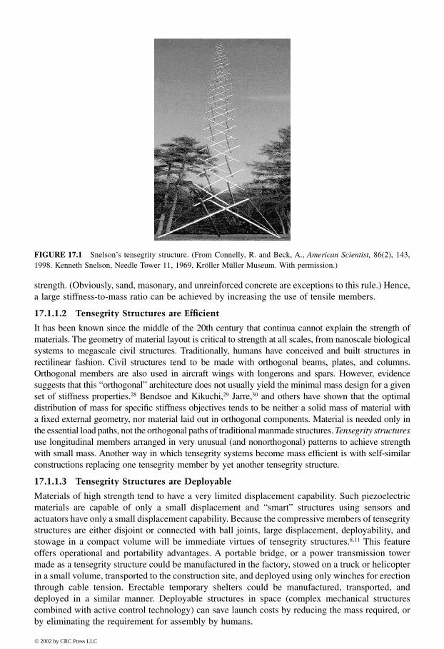
FIGURE 17.1

Snelson’s tensegrity structure. (From Connelly, R. and Beck, A.,

American Scientist,

86(2), 143,1998. Kenneth Snelson, Needle Tower 11, 1969, Kröller Müller Museum. With permission.)



17.1.1.4 Tensegrity Structures are Easily Tunable

The same deployment technique can also make small adjustments for fine tuning of the loadedstructures, or adjustment of a damaged structure. Structures that are designed to allow tuning will bean important feature of next generation mechanical structures, including civil engineering structures.

17.1.1.5 Tensegrity Structures Can be More Reliably Modeled

All members of a tensegrity structure are axially loaded. Perhaps the most promising scientificfeature of tensegrity structures is that while the

global

structure bends with external static loads,none of the

individual

members of the tensegrity structure experience bending moments. (In thischapter, we design all compressive members to experience loads well below their Euler bucklingloads.) Generally, members that experience deformation in two or three dimensions are much harderto model than members that experience deformation in only one dimension. The Euler bucklingload of a compressive member is from a bending instability calculation, and it is known in practiceto be very unreliable. That is, the actual buckling load measured from the test data has a largervariation and is not as predictable as the tensile strength. Hence, increased use of tensile membersis expected to yield more robust models and more efficient structures. More reliable models canbe expected for axially loaded members compared to models for members in bending.

31

17.1.1.6 Tensegrity Structures Facilitate High Precision Control

Structures that can be more precisely modeled can be more precisely controlled. Hence, tensegritystructures might open the door to quantum leaps in the precision of controlled structures. Thearchitecture (geometry) dictates the mathematical properties and, hence, these mathematical resultseasily scale from the nanoscale to the megascale, from applications in microsurgery to antennas,to aircraft wings, and to robotic manipulators.

17.1.1.7 Tensegrity is a Paradigm that Promotes the Integration of Structure and Control Disciplines

A given tensile or compressive member of a tensegrity structure can serve multiple functions. Itcan simultaneously be a load-carrying member of the structure, a sensor (measuring tension orlength), an actuator (such as nickel-titanium wire), a thermal insulator, or an electrical conductor.In other words, by proper choice of materials and geometry, a grand challenge awaits the tensegritydesigner: How to control the electrical, thermal, and mechanical energy in a material or structure?For example, smart tensegrity wings could use shape control to maneuver the aircraft or to optimizethe air foil as a function of flight condition, without the use of hinged surfaces. Tensegrity structuresprovide a promising paradigm for integrating structure and control design.

17.1.1.8 Tensegrity Structures are Motivated from Biology

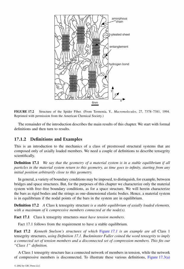
Figure 17.2 shows a rendition of a spider fiber, where amino acids of two types have formed hard

β−

pleated sheets that can take compression, and thin strands that take tension.

32,33

The

β−

pleatedsheets are discontinuous and the tension members form a continuous network. Hence, the nano-structure of the spider fiber is a tensegrity structure. Nature’s endorsement of tensegrity structureswarrants our attention because per unit mass, spider fiber is the strongest natural fiber.

Articles by Ingber

7,34,35

argue that tensegrity is the fundamental building architecture of life. Hisobservations come from experiments in cell biology, where prestressed truss structures of thetensegrity type have been observed in cells. It is encouraging to see the similarities in structuralbuilding blocks over a wide range of scales. If tensegrity is nature’s preferred building architecture,modern analytical and computational capabilities of tensegrity could make the same incredibleefficiency possessed by natural systems transferrable to manmade systems, from the nano- to themegascale. This is a grand design challenge, to develop scientific procedures to create smarttensegrity structures that can regulate the flow of thermal, mechanical, and electrical energy in amaterial system by proper choice of materials, geometry, and controls. This chapter contributes tothis cause by exploring the mechanical properties of simple tensegrity structures.



The remainder of the introduction describes the main results of this chapter. We start with formaldefinitions and then turn to results.

17.1.2 Definitions and Examples

This is an introduction to the mechanics of a class of prestressed structural systems that arecomposed only of axially loaded members. We need a couple of definitions to describe tensegrityscientifically.

Definition 17.1

We say that the geometry of a material system is in a stable equilibrium if allparticles in the material system return to this geometry, as time goes to infinity, starting from anyinitial position arbitrarily close to this geometry.

In general, a variety of boundary conditions may be imposed, to distinguish, for example, betweenbridges and space structures. But, for the purposes of this chapter we characterize only the materialsystem with free–free boundary conditions, as for a space structure. We will herein characterizethe bars as rigid bodies and the strings as one-dimensional elastic bodies. Hence, a material systemis in equilibrium if the nodal points of the bars in the system are in equilibrium.

Definition 17.2

A

Class k tensegrity structure

is a stable equilibrium of axially loaded elements,with a maximum of k compressive members connected at the node(s).

Fact 17.1

Class k tensegrity structures

must have tension members

.

Fact 17.1 follows from the requirement to have a stable equilibrium.

Fact 17.2

Kenneth Snelson’s structures of which

Figure

17.1 is an example are all

Class 1tensegrity structures,

using Definition 17.1. Buckminster Fuller coined the word tensegrity to implya connected set of tension members and a disconnected set of compression members. This fits our“Class 1” definition.

A Class 1 tensegrity structure has a connected network of members in tension, while the networkof compressive members is disconnected. To illustrate these various definitions, Figure 17.3(a)

FIGURE 17.2

Structure of the Spider Fiber. (From Termonia, Y.,

Macromolecules

, 27, 7378–7381, 1994.Reprinted with permission from the American Chemical Society.)

amorphouschain

β-pleated sheet

entanglement

hydrogen bond

yz

x6nm



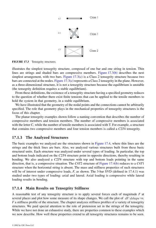
illustrates the simplest tensegrity structure, composed of one bar and one string in tension. Thinlines are strings and shaded bars are compressive members. Figure 17.3(b) describes the nextsimplest arrangement, with two bars. Figure 17.3(c) is a Class 2 tensegrity structure because twobars are connected at the nodes. Figure 17.3(c) represents a Class 2 tensegrity in the plane. However,as a three-dimensional structure, it is not a tensegrity structure because the equilibrium is unstable(the tensegrity definition requires a stable equilibrium).

From these definitions, the existence of a tensegrity structure having a specified geometry reducesto the question of whether there exist finite tensions that can be applied to the tensile members tohold the system in that geometry, in a stable equilibrium.

We have illustrated that the geometry of the nodal points and the connections cannot be arbitrarilyspecified. The role that geometry plays in the mechanical properties of tensegrity structures is thefocus of this chapter.

The planar tensegrity examples shown follow a naming convention that describes the number ofcompressive members and tension members. The number of compressive members is associatedwith the letter C, while the number of tensile members is associated with T. For example, a structurethat contains two compressive members and four tension members is called a

C

2

T

4 tensegrity.

17.1.3 The Analyzed Structures

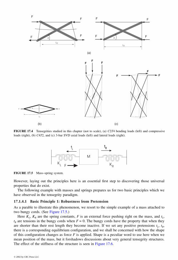
The basic examples we analyzed are the structures shown in Figure 17.4, where thin lines are thestrings and the thick lines are bars. Also, we analyzed various structures built from these basicstructural units. Each structure was analyzed under several types of loading. In particular, the topand bottom loads indicated on the

C

2

T

4 structure point in opposite directions, thereby resulting inbending. We also analyzed a

C

2

T

4 structure with top and bottom loads pointing in the samedirection, that is, a compressive situation. The

C

4

T

2 structure of Figure 17.4(b) reduces to a

C

4

T

1structure when the horizontal string is absent. The mass and stiffness properties of such structureswill be of interest under compressive loads,

F

, as shown. The 3-bar SVD (defined in 17.4.1) wasstudied under two types of loading: axial and lateral. Axial loading is compressive while lateralloading results in bending.

17.1.4 Main Results on Tensegrity Stiffness

A reasonable test of any tensegrity structure is to apply several forces each of magnitude

F

atseveral places and plot how some measure of its shape changes. We call the plot of vs.

F

a stiffness profile of the structure. The chapter analyzes stiffness profiles of a variety of tensegritystructures. We paid special attention to the role of pretension set in the strings of the tensegrity.While we have not done an exhaustive study, there are properties common to these examples whichwe now describe. How well these properties extend to all tensegrity structures remains to be seen.

FIGURE 17.3

Tensegrity structures.

dF dshape



However, laying out the principles here is an essential first step to discovering those universalproperties that do exist.

The following example with masses and springs prepares us for two basic principles which wehave observed in the tensegrity paradigm.

17.1.4.1 Basic Principle 1: Robustness from Pretension

As a parable to illustrate this phenomenon, we resort to the simple example of a mass attached totwo bungy cords. (See Figure 17.5.)

Here

K

L

,

K

R

are the spring constants,

F

is an external force pushing right on the mass, and

t

L

,

t

R

are tensions in the bungy cords when

F

= 0. The bungy cords have the property that when theyare shorter than their rest length they become inactive. If we set any positive pretensions

t

L

,

t

R

,there is a corresponding equilibrium configuration, and we shall be concerned with how the shapeof this configuration changes as force

F

is applied. Shape is a peculiar word to use here when wemean position of the mass, but it forshadows discussions about very general tensegrity structures.The effect of the stiffness of the structure is seen in Figure 17.6.

FIGURE 17.4

Tensegrities studied in this chapter (not to scale), (a)

C

2

T

4 bending loads (left) and compressiveloads (right), (b)

C

4

T

2, and (c) 3-bar SVD axial loads (left) and lateral loads (right).

FIGURE 17.5

Mass–spring system.

(a)

(b) (c)



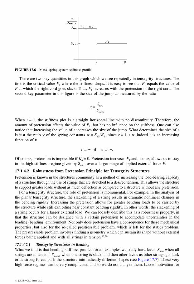
There are two key quantities in this graph which we see repeatedly in tensegrity structures. Thefirst is the critical value F1 where the stiffness drops. It is easy to see that F1 equals the value ofF at which the right cord goes slack. Thus, F1 increases with the pretension in the right cord. Thesecond key parameter in this figure is the size of the jump as measured by the ratio

When r = 1, the stiffness plot is a straight horizontal line with no discontinuity. Therefore, theamount of pretension affects the value of F1, but has no influence on the stiffness. One can alsonotice that increasing the value of r increases the size of the jump. What determines the size of ris just the ratio κ of the spring constants , since r = 1 + κ, indeed r is an increasingfunction of κ

r ≅ ∞ if κ ≅ ∞.

Of course, pretension is impossible if KR = 0. Pretension increases F1 and, hence, allows us to stayin the high stiffness regime given by Stens, over a larger range of applied external force F.

17.1.4.2 Robustness from Pretension Principle for Tensegrity Structures

Pretension is known in the structures community as a method of increasing the load-bearing capacityof a structure through the use of strings that are stretched to a desired tension. This allows the structureto support greater loads without as much deflection as compared to a structure without any pretension.

For a tensegrity structure, the role of pretension is monumental. For example, in the analysis ofthe planar tensegrity structure, the slackening of a string results in dramatic nonlinear changes inthe bending rigidity. Increasing the pretension allows for greater bending loads to be carried bythe structure while still exhibiting near constant bending rigidity. In other words, the slackening ofa string occurs for a larger external load. We can loosely describe this as a robustness property, inthat the structure can be designed with a certain pretension to accomodate uncertainties in theloading (bending) environment. Not only does pretension have a consequence for these mechanicalproperties, but also for the so-called prestressable problem, which is left for the statics problem.The prestressable problem involves finding a geometry which can sustain its shape without externalforces being applied and with all strings in tension.12,20

17.1.4.2.1 Tensegrity Structures in BendingWhat we find is that bending stiffness profiles for all examples we study have levels Stens when allstrings are in tension, Sslack1 when one string is slack, and then other levels as other strings go slackor as strong forces push the structure into radically different shapes (see Figure 17.7). These veryhigh force regimes can be very complicated and so we do not analyze them. Loose motivation for

FIGURE 17.6 Mass–spring system stiffness profile.

rS

Stens

slack

:=

κ:= K KR L



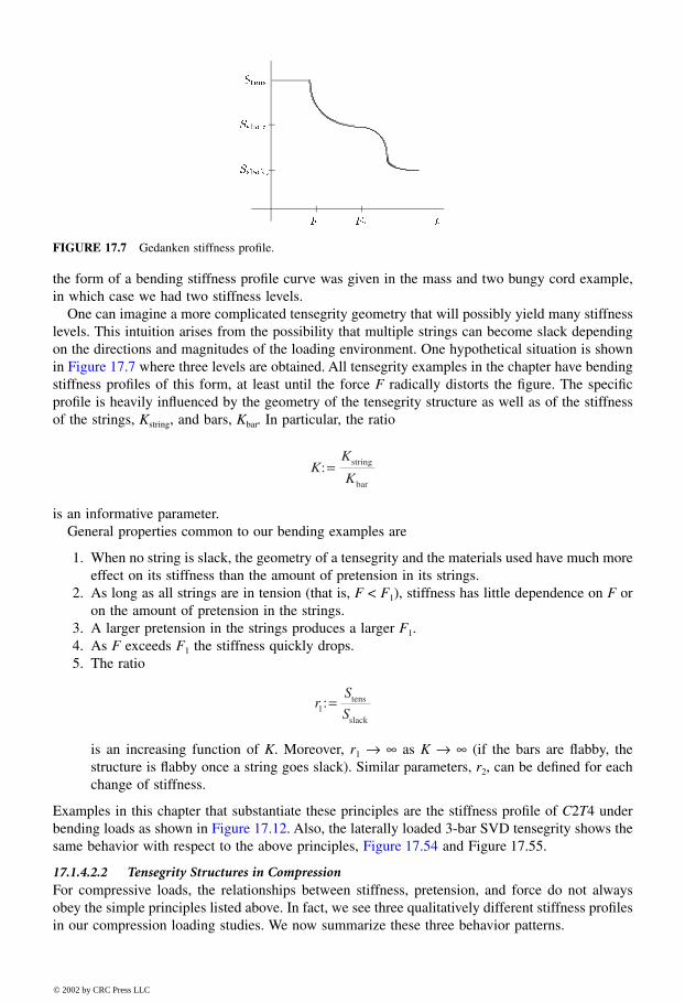
the form of a bending stiffness profile curve was given in the mass and two bungy cord example,in which case we had two stiffness levels.

One can imagine a more complicated tensegrity geometry that will possibly yield many stiffnesslevels. This intuition arises from the possibility that multiple strings can become slack dependingon the directions and magnitudes of the loading environment. One hypothetical situation is shownin Figure 17.7 where three levels are obtained. All tensegrity examples in the chapter have bendingstiffness profiles of this form, at least until the force F radically distorts the figure. The specificprofile is heavily influenced by the geometry of the tensegrity structure as well as of the stiffnessof the strings, Kstring, and bars, Kbar. In particular, the ratio

is an informative parameter.General properties common to our bending examples are

1. When no string is slack, the geometry of a tensegrity and the materials used have much moreeffect on its stiffness than the amount of pretension in its strings.

2. As long as all strings are in tension (that is, F < F1), stiffness has little dependence on F oron the amount of pretension in the strings.

3. A larger pretension in the strings produces a larger F1.4. As F exceeds F1 the stiffness quickly drops.5. The ratio

is an increasing function of K. Moreover, r1 → ∞ as K → ∞ (if the bars are flabby, thestructure is flabby once a string goes slack). Similar parameters, r2, can be defined for eachchange of stiffness.

Examples in this chapter that substantiate these principles are the stiffness profile of C2T4 underbending loads as shown in Figure 17.12. Also, the laterally loaded 3-bar SVD tensegrity shows thesame behavior with respect to the above principles, Figure 17.54 and Figure 17.55.

17.1.4.2.2 Tensegrity Structures in CompressionFor compressive loads, the relationships between stiffness, pretension, and force do not alwaysobey the simple principles listed above. In fact, we see three qualitatively different stiffness profilesin our compression loading studies. We now summarize these three behavior patterns.

FIGURE 17.7 Gedanken stiffness profile.

KK

K:= string

bar

rS

S1:= tens

slack



The C2T4 planar tensegrity exhibits the pretension robustness properties of Principles I, II, III,as shown in Figure 17.6. The pretension tends to prevent slack strings.

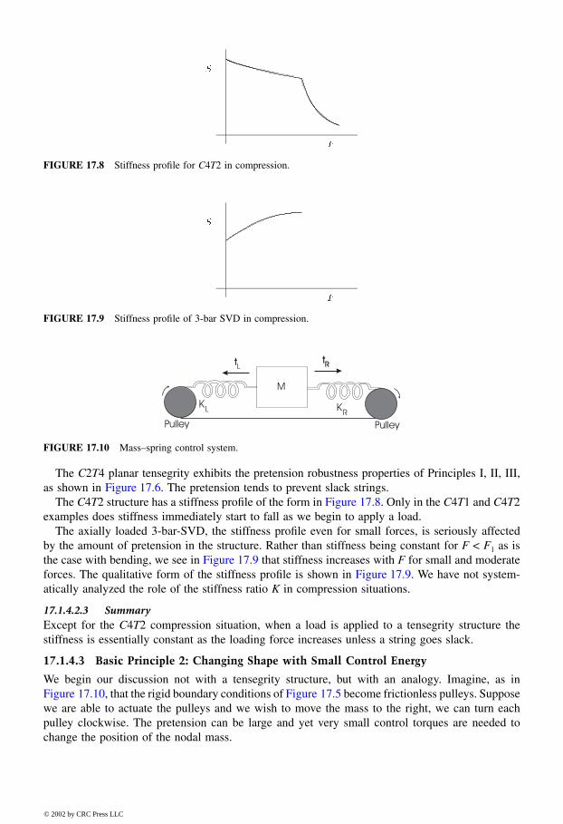
The C4T2 structure has a stiffness profile of the form in Figure 17.8. Only in the C4T1 and C4T2examples does stiffness immediately start to fall as we begin to apply a load.

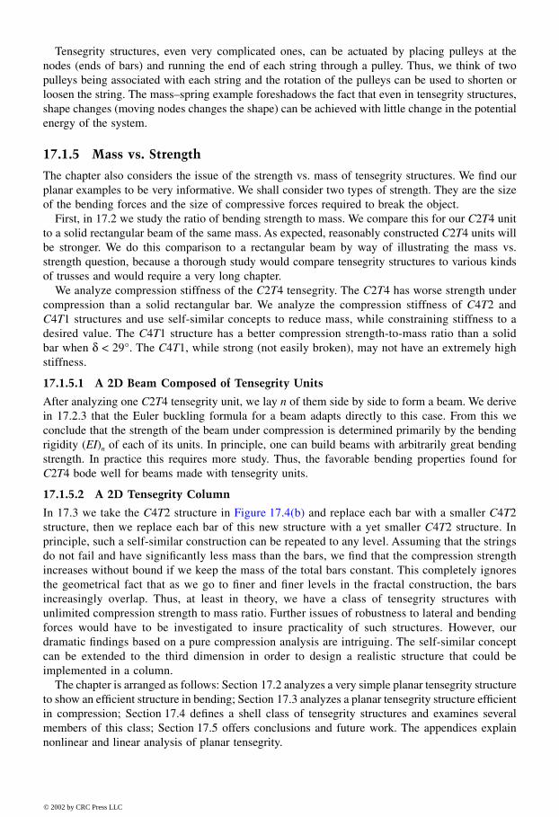
The axially loaded 3-bar-SVD, the stiffness profile even for small forces, is seriously affectedby the amount of pretension in the structure. Rather than stiffness being constant for F < F1 as isthe case with bending, we see in Figure 17.9 that stiffness increases with F for small and moderateforces. The qualitative form of the stiffness profile is shown in Figure 17.9. We have not system-atically analyzed the role of the stiffness ratio K in compression situations.

17.1.4.2.3 SummaryExcept for the C4T2 compression situation, when a load is applied to a tensegrity structure thestiffness is essentially constant as the loading force increases unless a string goes slack.

17.1.4.3 Basic Principle 2: Changing Shape with Small Control Energy

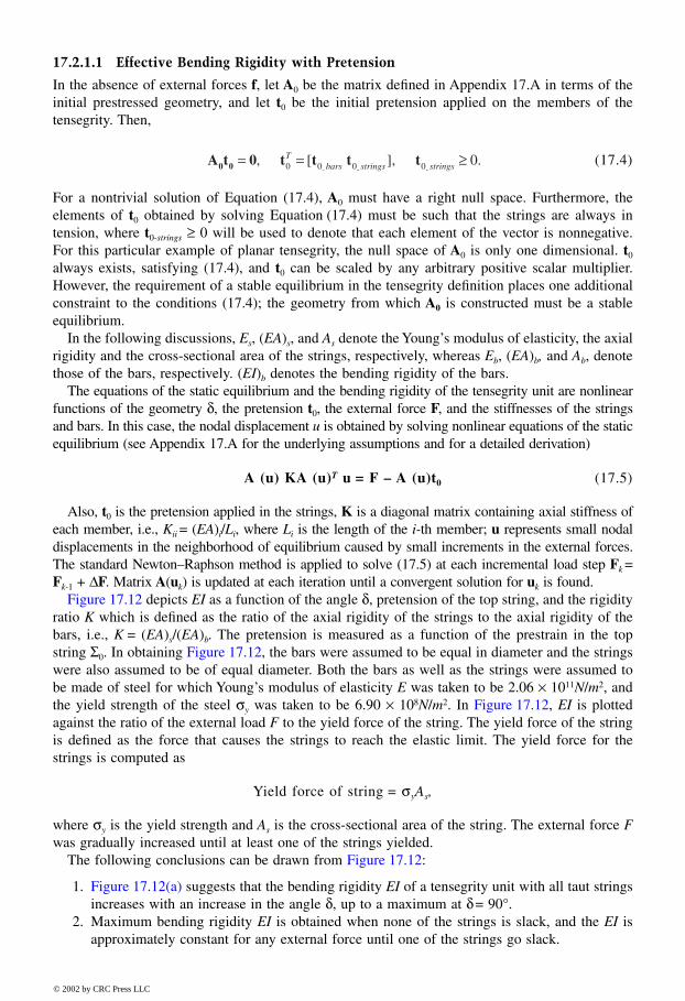
We begin our discussion not with a tensegrity structure, but with an analogy. Imagine, as inFigure 17.10, that the rigid boundary conditions of Figure 17.5 become frictionless pulleys. Supposewe are able to actuate the pulleys and we wish to move the mass to the right, we can turn eachpulley clockwise. The pretension can be large and yet very small control torques are needed tochange the position of the nodal mass.

FIGURE 17.8 Stiffness profile for C4T2 in compression.

FIGURE 17.9 Stiffness profile of 3-bar SVD in compression.

FIGURE 17.10 Mass–spring control system.



Tensegrity structures, even very complicated ones, can be actuated by placing pulleys at thenodes (ends of bars) and running the end of each string through a pulley. Thus, we think of twopulleys being associated with each string and the rotation of the pulleys can be used to shorten orloosen the string. The mass–spring example foreshadows the fact that even in tensegrity structures,shape changes (moving nodes changes the shape) can be achieved with little change in the potentialenergy of the system.

17.1.5 Mass vs. Strength

The chapter also considers the issue of the strength vs. mass of tensegrity structures. We find ourplanar examples to be very informative. We shall consider two types of strength. They are the sizeof the bending forces and the size of compressive forces required to break the object.

First, in 17.2 we study the ratio of bending strength to mass. We compare this for our C2T4 unitto a solid rectangular beam of the same mass. As expected, reasonably constructed C2T4 units willbe stronger. We do this comparison to a rectangular beam by way of illustrating the mass vs.strength question, because a thorough study would compare tensegrity structures to various kindsof trusses and would require a very long chapter.

We analyze compression stiffness of the C2T4 tensegrity. The C2T4 has worse strength undercompression than a solid rectangular bar. We analyze the compression stiffness of C4T2 andC4T1 structures and use self-similar concepts to reduce mass, while constraining stiffness to adesired value. The C4T1 structure has a better compression strength-to-mass ratio than a solidbar when δ < 29°. The C4T1, while strong (not easily broken), may not have an extremely highstiffness.

17.1.5.1 A 2D Beam Composed of Tensegrity Units

After analyzing one C2T4 tensegrity unit, we lay n of them side by side to form a beam. We derivein 17.2.3 that the Euler buckling formula for a beam adapts directly to this case. From this weconclude that the strength of the beam under compression is determined primarily by the bendingrigidity (EI)n of each of its units. In principle, one can build beams with arbitrarily great bendingstrength. In practice this requires more study. Thus, the favorable bending properties found forC2T4 bode well for beams made with tensegrity units.

17.1.5.2 A 2D Tensegrity Column

In 17.3 we take the C4T2 structure in Figure 17.4(b) and replace each bar with a smaller C4T2structure, then we replace each bar of this new structure with a yet smaller C4T2 structure. Inprinciple, such a self-similar construction can be repeated to any level. Assuming that the stringsdo not fail and have significantly less mass than the bars, we find that the compression strengthincreases without bound if we keep the mass of the total bars constant. This completely ignoresthe geometrical fact that as we go to finer and finer levels in the fractal construction, the barsincreasingly overlap. Thus, at least in theory, we have a class of tensegrity structures withunlimited compression strength to mass ratio. Further issues of robustness to lateral and bendingforces would have to be investigated to insure practicality of such structures. However, ourdramatic findings based on a pure compression analysis are intriguing. The self-similar conceptcan be extended to the third dimension in order to design a realistic structure that could beimplemented in a column.

The chapter is arranged as follows: Section 17.2 analyzes a very simple planar tensegrity structureto show an efficient structure in bending; Section 17.3 analyzes a planar tensegrity structure efficientin compression; Section 17.4 defines a shell class of tensegrity structures and examines severalmembers of this class; Section 17.5 offers conclusions and future work. The appendices explainnonlinear and linear analysis of planar tensegrity.



17.2 Planar Tensegrity Structures Efficient in Bending

In this section, we examine the bending rigidity of a single tensegrity unit, a planar tensegritymodel under pure bending as shown in Figure 17.11, where thin lines are the four strings and thetwo thick lines are bars. Because the structure in Figure 17.11 has two compressive and four tensilemembers, we refer to it as a C2T4 structure.

17.2.1 Bending Rigidity of a Single Tensegrity Unit

To arrive at a definition of bending stiffness suitable to C2T4, note that the moment M acting onthe section is given by

M = FLbar sin δ, (17.1)

where F is the magnitude of the external force, Lbar is the length of the bar, and δ is the angle thatthe bars make with strings in the deformed state, as shown in Figure 17.11.

In Figure 17.11, ρ is the radius of curvature of the tensegrity unit under bending deformation.It can be shown from Figure 17.11 that

(17.2)

The bending rigidity is defined by EI = Mρ. Hence,

(17.3)

where EI is the equivalent bending rigidity of the planar one-stage tensegrity unit and u is the nodaldisplacement. The evaluation of the bending rigidity of the planar unit requires the evaluation ofu, which will follow under various hypotheses. The bending rigidity will later be obtained bysubstituting u in (17.3).

FIGURE 17.11 Planar one-stage tensegrity unit under pure bending.

ρ δ δ δ θ=

=L

uu Lbar

bar212

2

cos sin 1

sin tan .,

EI FL FLL

ubar barbar= =

sin sin cos 12δρ δ δ

2

2

.



17.2.1.1 Effective Bending Rigidity with Pretension

In the absence of external forces f, let A0 be the matrix defined in Appendix 17.A in terms of theinitial prestressed geometry, and let t0 be the initial pretension applied on the members of thetensegrity. Then,

(17.4)

For a nontrivial solution of Equation (17.4), A0 must have a right null space. Furthermore, theelements of t0 obtained by solving Equation (17.4) must be such that the strings are always intension, where t0-strings ≥ 0 will be used to denote that each element of the vector is nonnegative.For this particular example of planar tensegrity, the null space of A0 is only one dimensional. t0

always exists, satisfying (17.4), and t0 can be scaled by any arbitrary positive scalar multiplier.However, the requirement of a stable equilibrium in the tensegrity definition places one additionalconstraint to the conditions (17.4); the geometry from which A0 is constructed must be a stableequilibrium.

In the following discussions, Es, (EA)s, and As denote the Young’s modulus of elasticity, the axialrigidity and the cross-sectional area of the strings, respectively, whereas Eb, (EA)b, and Ab, denotethose of the bars, respectively. (EI)b denotes the bending rigidity of the bars.

The equations of the static equilibrium and the bending rigidity of the tensegrity unit are nonlinearfunctions of the geometry δ, the pretension t0, the external force F, and the stiffnesses of the stringsand bars. In this case, the nodal displacement u is obtained by solving nonlinear equations of the staticequilibrium (see Appendix 17.A for the underlying assumptions and for a detailed derivation)

A (u) KA (u)T u = F – A (u)t0 (17.5)

Also, t0 is the pretension applied in the strings, K is a diagonal matrix containing axial stiffness ofeach member, i.e., Kii = (EA)i/Li, where Li is the length of the i-th member; u represents small nodaldisplacements in the neighborhood of equilibrium caused by small increments in the external forces.The standard Newton–Raphson method is applied to solve (17.5) at each incremental load step Fk =Fk-1 + ∆F. Matrix A(uk) is updated at each iteration until a convergent solution for uk is found.

Figure 17.12 depicts EI as a function of the angle δ, pretension of the top string, and the rigidityratio K which is defined as the ratio of the axial rigidity of the strings to the axial rigidity of thebars, i.e., K = (EA)s/(EA)b. The pretension is measured as a function of the prestrain in the topstring Σ0. In obtaining Figure 17.12, the bars were assumed to be equal in diameter and the stringswere also assumed to be of equal diameter. Both the bars as well as the strings were assumed tobe made of steel for which Young’s modulus of elasticity E was taken to be 2.06 × 1011N/m2, andthe yield strength of the steel σy was taken to be 6.90 × 108N/m2. In Figure 17.12, EI is plottedagainst the ratio of the external load F to the yield force of the string. The yield force of the stringis defined as the force that causes the strings to reach the elastic limit. The yield force for thestrings is computed as

Yield force of string = σyAs,

where σy is the yield strength and As is the cross-sectional area of the string. The external force Fwas gradually increased until at least one of the strings yielded.

The following conclusions can be drawn from Figure 17.12:

1. Figure 17.12(a) suggests that the bending rigidity EI of a tensegrity unit with all taut stringsincreases with an increase in the angle δ, up to a maximum at δ = 90°.

2. Maximum bending rigidity EI is obtained when none of the strings is slack, and the EI isapproximately constant for any external force until one of the strings go slack.

A t 0 t t t t0 0 = = ≥, [ ], . 0 0 0- - -0 0T

bars strings strings



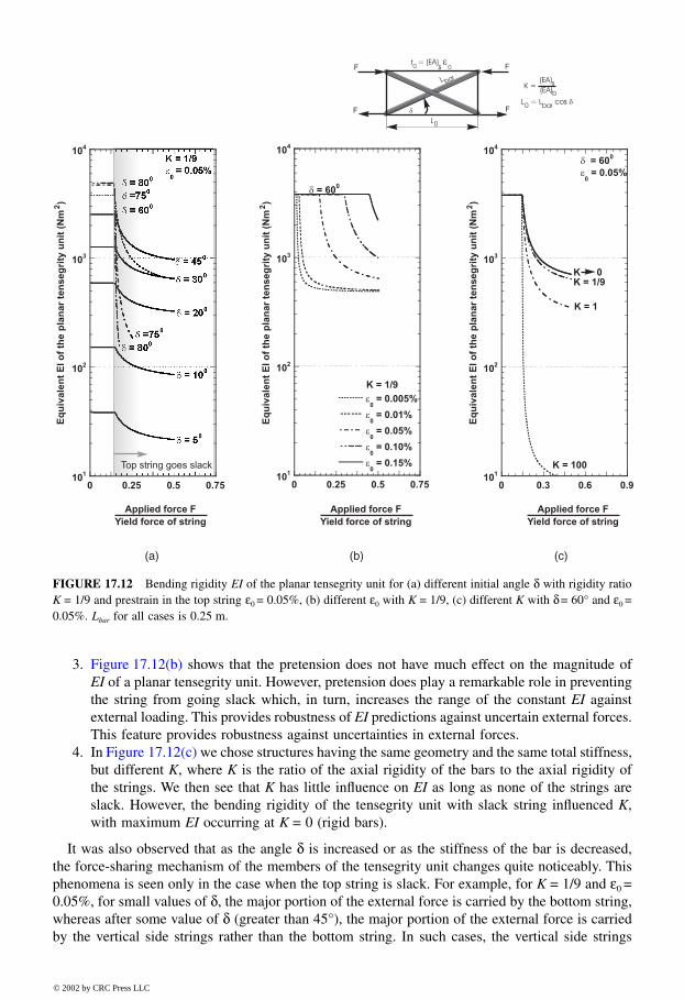
3. Figure 17.12(b) shows that the pretension does not have much effect on the magnitude ofEI of a planar tensegrity unit. However, pretension does play a remarkable role in preventingthe string from going slack which, in turn, increases the range of the constant EI againstexternal loading. This provides robustness of EI predictions against uncertain external forces.This feature provides robustness against uncertainties in external forces.

4. In Figure 17.12(c) we chose structures having the same geometry and the same total stiffness,but different K, where K is the ratio of the axial rigidity of the bars to the axial rigidity ofthe strings. We then see that K has little influence on EI as long as none of the strings areslack. However, the bending rigidity of the tensegrity unit with slack string influenced K,with maximum EI occurring at K = 0 (rigid bars).

It was also observed that as the angle δ is increased or as the stiffness of the bar is decreased,the force-sharing mechanism of the members of the tensegrity unit changes quite noticeably. Thisphenomena is seen only in the case when the top string is slack. For example, for K = 1/9 and ε0 =0.05%, for small values of δ, the major portion of the external force is carried by the bottom string,whereas after some value of δ (greater than 45°), the major portion of the external force is carriedby the vertical side strings rather than the bottom string. In such cases, the vertical side strings

FIGURE 17.12 Bending rigidity EI of the planar tensegrity unit for (a) different initial angle δ with rigidity ratioK = 1/9 and prestrain in the top string ε0 = 0.05%, (b) different ε0 with K = 1/9, (c) different K with δ = 60° and ε0 =0.05%. Lbar for all cases is 0.25 m.

(a) (b) (c)



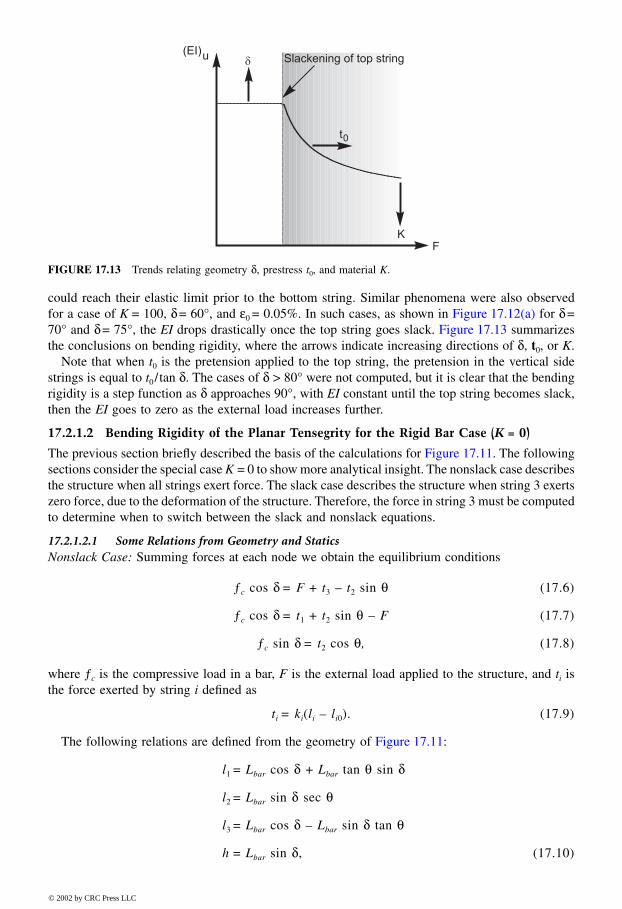
could reach their elastic limit prior to the bottom string. Similar phenomena were also observedfor a case of K = 100, δ = 60°, and ε0 = 0.05%. In such cases, as shown in Figure 17.12(a) for δ =70° and δ = 75°, the EI drops drastically once the top string goes slack. Figure 17.13 summarizesthe conclusions on bending rigidity, where the arrows indicate increasing directions of δ, t0, or K.

Note that when t0 is the pretension applied to the top string, the pretension in the vertical sidestrings is equal to t0/tan δ. The cases of δ > 80° were not computed, but it is clear that the bendingrigidity is a step function as δ approaches 90°, with EI constant until the top string becomes slack,then the EI goes to zero as the external load increases further.

17.2.1.2 Bending Rigidity of the Planar Tensegrity for the Rigid Bar Case (K = 0)

The previous section briefly described the basis of the calculations for Figure 17.11. The followingsections consider the special case K = 0 to show more analytical insight. The nonslack case describesthe structure when all strings exert force. The slack case describes the structure when string 3 exertszero force, due to the deformation of the structure. Therefore, the force in string 3 must be computedto determine when to switch between the slack and nonslack equations.

17.2.1.2.1 Some Relations from Geometry and StaticsNonslack Case: Summing forces at each node we obtain the equilibrium conditions

ƒc cos δ = F + t3 – t2 sin θ (17.6)

ƒc cos δ = t1 + t2 sin θ – F (17.7)

ƒc sin δ = t2 cos θ, (17.8)

where ƒc is the compressive load in a bar, F is the external load applied to the structure, and ti isthe force exerted by string i defined as

ti = ki(li – li0). (17.9)

The following relations are defined from the geometry of Figure 17.11:

l1 = Lbar cos δ + Lbar tan θ sin δ

l2 = Lbar sin δ sec θ

l3 = Lbar cos δ – Lbar sin δ tan θ

h = Lbar sin δ, (17.10)

FIGURE 17.13 Trends relating geometry δ, prestress t0, and material K.



where li denote the geometric length of the strings. We will find the relation between δ and θ byeliminating fc and F from (17.6)–(17.8)

(17.11)

Substitution of relations (17.10) and (17.9) into (17.11) yields

(17.12)

If ki = k, then (17.12) simplifies to

(17.13)

Slack Case: In order to find a relation between δ and θ for the slack case when t3 has zerotension, we use (17.12) and set k3 to zero. With the simplification that we use the same materialproperties, we obtain

0 = Lbar tan θ sin δ tan δ + 2l20 cos θ – l10 tan δ – Lbar sin δ. (17.14)

This relationship between δ and θ will be used in (17.22) to describe bending rigidity.

17.2.1.2.2 Bending Rigidity EquationsThe bending rigidity is defined in (17.3) in terms of ρ and F. Now we will solve the geometric andstatic equations for ρ and F in terms of the parameters θ, δ of the structure. For the nonslack case,we will use (17.13) to get an analytical formula for the EI. For the slack case, we do not have ananalytical formula. Hence, this must be done numerically.

From geometry, we can obtain ρ,

Solving for ρ we obtain

(17.15)

Nonslack Case: In the nonslack case, we now apply the relation in (17.13) to simplify (17.15)

(17.16)

cos tan .θ δ=+t t

t1 3

22

cos( cos tan sin ) ( cos tan sin )

( sin sec )tan

+ .θ

δ θ δ δ θ δδ θ

δ=− + − −

−k L L l k L L l

k L lbar bar bar bar

bar

1 10 3 30

2 202

tan δ θ β θ=+

2 20

10 30

l

l lcos = cos .

tan( )

θρ

=+

lh

1

22.

ρθ

δ θ δθ

δ

δθ

= −

+−

=

l h

L L L

L

bar bar bar

bar

1

2 2

2 2

2

tan

cos tan sin

tan

sin

costan

.

=

ρθ β θ

=+

Lbar

21

1 2 2tan cos.



From (17.6)–(17.8) we can solve for the equilibrium external F

– k3 Lbar cos δ + k3 Lbar sin δ tan θ + k3l30). (17.17)

Again, using (17.13) and ki = k, Equation (17.17) simplifies to

(17.18)

We can substitute (17.18) and (17.16) into (17.3)

(17.19)

and we obtain the bending rigidity of the planar structure with no slack strings present. Theexpression for string length l3 in the nonslack case reduces to

(17.20)

This expression can be used to determine the angle which causes l3 to become slack.Slack Case: Similarly, for the case when string 3 goes slack, we set k3 = 0 and ki = k in (17.17),

which yield simply

(17.21)

and

(17.22)

See Figure 17.12(c) for a plot of EI for the K = 0 (rigid bar) case.

17.2.1.2.3 Constants and ConversionsAll plots shown are generated with the following data which can then be converted as follows ifnecessary.

F t t t

k L k L k l

k L k l

bar bar

bar

= + −

= + −

+ −

12

2

12

2 2

1 2 3

1 1 1 10

2 2 20

( sin )

( cos tan sin

sin tan sin

θ

δ θ δ

δ θ θ

FkL k

l l lbar=+

− −2

1 22

2 2 10 30 20

β θβ θ

θsin

cossin ( + ).

ElL kL k

l l lbar bar=+ +

− −

2 2

2 2 2 2 10 30 202 1

2

1 22

β θβ θ θ

β θβ θ

θcos

( cos ) (sin )

sin

cossin , ( + )

l Lbar3 2 2

= 1 + cos

1− β θβ θ sin

.

F t t

kL kL kl kl

slack

bar bar

= ( + )

= (

12

2

12

3 2

1 2

10 20

sin

cos tan sin sin )

θ

δ θ δ θ+ − −

EIL

kL kL kl klslackbar

bar bar=

( 2

10 2043 2

sin cos

tancos tan sin sin ).

δ δθ

δ θ δ θ+ − −



Young’s Modulus, E = 2.06 × 1011 N/m2

Yield Stress, σ = 6.9 × 108 N/m2

Diameter of Tendons = 1 mm

Cross-Sectional Area of Tendon = 7.8540 × 10–7 m2

Length of Bar, Lbar = .25 m

Prestress = e0

Initial Angle = δ0

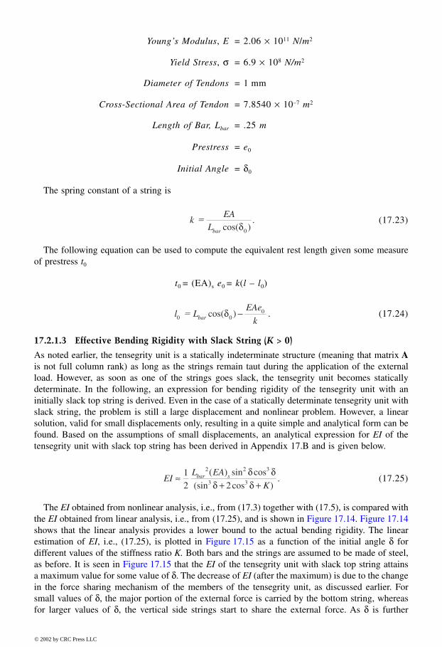
The spring constant of a string is

(17.23)

The following equation can be used to compute the equivalent rest length given some measureof prestress t0

t0 = (EA)s e0 = k(l – l0)

. (17.24)

17.2.1.3 Effective Bending Rigidity with Slack String (K > 0)

As noted earlier, the tensegrity unit is a statically indeterminate structure (meaning that matrix Ais not full column rank) as long as the strings remain taut during the application of the externalload. However, as soon as one of the strings goes slack, the tensegrity unit becomes staticallydeterminate. In the following, an expression for bending rigidity of the tensegrity unit with aninitially slack top string is derived. Even in the case of a statically determinate tensegrity unit withslack string, the problem is still a large displacement and nonlinear problem. However, a linearsolution, valid for small displacements only, resulting in a quite simple and analytical form can befound. Based on the assumptions of small displacements, an analytical expression for EI of thetensegrity unit with slack top string has been derived in Appendix 17.B and is given below.

(17.25)

The EI obtained from nonlinear analysis, i.e., from (17.3) together with (17.5), is compared withthe EI obtained from linear analysis, i.e., from (17.25), and is shown in Figure 17.14. Figure 17.14shows that the linear analysis provides a lower bound to the actual bending rigidity. The linearestimation of EI, i.e., (17.25), is plotted in Figure 17.15 as a function of the initial angle δ fordifferent values of the stiffness ratio K. Both bars and the strings are assumed to be made of steel,as before. It is seen in Figure 17.15 that the EI of the tensegrity unit with slack top string attainsa maximum value for some value of δ. The decrease of EI (after the maximum) is due to the changein the force sharing mechanism of the members of the tensegrity unit, as discussed earlier. Forsmall values of δ, the major portion of the external force is carried by the bottom string, whereasfor larger values of δ, the vertical side strings start to share the external force. As δ is further

k

EALbar

=cos( )

.δ0

l LEAe

kbar0 00 = cos( )δ −

EIL EA

Kbar s≈

+ +12 2

2 2 3

3 3

( ) sin cos

(sin cos ).

δ δδ δ



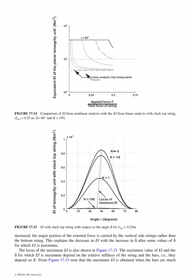
increased, the major portion of the external force is carried by the vertical side strings rather thanthe bottom string. This explains the decrease in EI with the increase in δ after some values of δfor which EI is maximum.

The locus of the maximum EI is also shown in Figure 17.15. The maximum value of EI and theδ for which EI is maximum depend on the relative stiffness of the string and the bars, i.e., theydepend on K. From Figure 17.15 note that the maximum EI is obtained when the bars are much

FIGURE 17.14 Comparison of EI from nonlinear analysis with the EI from linear analysis with slack top string(Lbar = 0.25 m, δ = 60° and K = 1/9).

FIGURE 17.15 EI with slack top string with respect to the angle δ for Lbar = 0.25m.



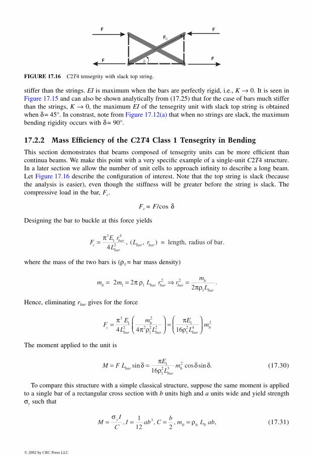
stiffer than the strings. EI is maximum when the bars are perfectly rigid, i.e., K → 0. It is seen inFigure 17.15 and can also be shown analytically from (17.25) that for the case of bars much stifferthan the strings, K → 0, the maximum EI of the tensegrity unit with slack top string is obtainedwhen δ = 45°. In constrast, note from Figure 17.12(a) that when no strings are slack, the maximumbending rigidity occurs with δ = 90°.

17.2.2 Mass Efficiency of the C2T4 Class 1 Tensegrity in Bending

This section demonstrates that beams composed of tensegrity units can be more efficient thancontinua beams. We make this point with a very specific example of a single-unit C2T4 structure.In a later section we allow the number of unit cells to approach infinity to describe a long beam.Let Figure 17.16 describe the configuration of interest. Note that the top string is slack (becausethe analysis is easier), even though the stiffness will be greater before the string is slack. Thecompressive load in the bar, Fc.

Fc = F/cos δ

Designing the bar to buckle at this force yields

where the mass of the two bars is (ρ1 = bar mass density)

Hence, eliminating rbar gives for the force

The moment applied to the unit is

(17.30)

To compare this structure with a simple classical structure, suppose the same moment is appliedto a single bar of a rectangular cross section with b units high and a units wide and yield strengthσy such that

(17.31)

FIGURE 17.16 C2T4 tensegrity with slack top string.

FE r

LL rc

bar

barbar bar=

π31

4

24

( = length, radius of bar, , ) .

m m L r rm

Lb bar bar barb

bar

= = ⇒ = 2 221 1

2 2

1

π ρπρ

.

F

E

L

m

L

E

Lmc

bar

b

bar barb=

=

ππ ρ

πρ

31

2

2

212 2

1

12 4

2

4 4 16

M F LE

Lmbar

barb= =sin cos sin .δ π

ρδ δ1

12 3

2

16

M

II ab C

bm L aby= = = =

σρ

C, , , ,

112 2

300 0



then, for the rectangular bar

(17.32)

Equating (17.30) and (17.32), using L0 = Lbar cos δ, yields the material/geometry conservationlaw ( is a material property and g is a property of the geometry)

(17.33)

The mass ratio µ is infinity if δ = 0°, 90°, and the lower bound on the mass ratio is achievedwhen = 26.565°.

Lemma 17.1 Let σy denote the yield stress of a bar with modulus of elasticity E1 and dimensiona × b × L0. Let M denote the bending moment about an axis perpendicular to the b dimension. Mis the moment at which the bar fails in bending. Then, the C2T4 tensegrity fails at the same M buthas less mass if and minimal mass is achieved at .

Proof: From (17.33),

(17.34)

where the lower bound is achieved at by setting ∂g/∂δ = 0 and solvingcos2 δ = 4sin2 δ, or tan δ = 1/2. ❏

For steel with (σy , E1) = (6.9 × 108, 2 × 1011)

(17.35)

where the lower bound is achieved for = 26.565°. Hence, for geometry of the steelcomparison bar given by then mb = 0.51 m0, showing49% improvemen t i n mas s f o r a g iven y i e ld momen t . Fo r t he geome t ry

, mb = 0.2m0, showing 80% improvement in mass for a given yieldmoment, M. The main point here is that strength and mass efficiency are achieved by geometry(δ = 26.565°), not materials.

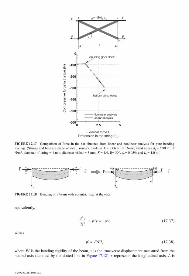
It can be shown that the compressive force in a bar when the system C2T4 is under a purebending load exhibits a similar robustness property that was shown with the bending rigidity. Theforce in a bar is constant until a string becomes slack, which is shown in Figure 17.17.

17.2.3 Global Bending of a Beam Made from C2T4 Units

The question naturally arises “what is the bending rigidity of a beam made from many tensegritycells?” 17.2.3.2 answers that question. First, in Section 17.2.3.1 we review the standard beam theory.

17.2.3.1 Bucklings Load

For a beam loaded as shown in Figure 17.18, we have

(17.36)

M

m

a Ly=

σρ

02

02

026

.

σ

µ δ

πσ σ

σδ δ

2 0

=

= = =∆ ∆ ∆m

mg

Eg

L

ab y

2

1

043

, ,cos sin

δ = −tan ( )1 1 2

σg < ( ),3π δ δ = −tan ( )1 1 2

µ δπ

σ δπ

σ2 0

3 33 493856= ≥ =g g g

L

a, , .

( )δ π σ3 g δ = −tan ( )1 1 2

( ),N m2

µ δ

πσ2 = ≥

30 008035869 0g

L

a.

tan ( )−1 1 2L a o

0150 1 2 26 565= = ={ }−, tan ( ) . ,and δ

L a0

o= ={ }20 26 565and δ .

EI

d v

dzFv Fe

2

2 = − −



equivalently,

(17.37)

where

p2 = F/EI, (17.38)

where EI is the bending rigidity of the beam, v is the transverse displacement measured from theneutral axis (denoted by the dotted line in Figure 17.18), z represents the longitudinal axis, L is

FIGURE 17.17 Comparison of force in the bar obtained from linear and nonlinear analysis for pure bendingloading. (Strings and bars are made of steel, Young’s modulus E = 2.06 × 1011 N/m2, yield stress σy = 6.90 × 108

N/m2, diameter of string = 1 mm, diameter of bar = 3 mm, K = 1/9, δ = 30°, ε0 = 0.05% and L0 = 1.0 m.)

FIGURE 17.18 Bending of a beam with eccentric load at the ends.

d v

dzp v p e

2

22 2 + = −



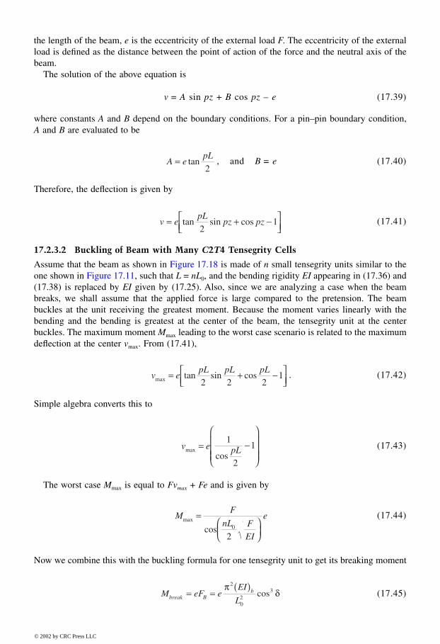
the length of the beam, e is the eccentricity of the external load F. The eccentricity of the externalload is defined as the distance between the point of action of the force and the neutral axis of thebeam.

The solution of the above equation is

v = A sin pz + B cos pz – e (17.39)

where constants A and B depend on the boundary conditions. For a pin–pin boundary condition,A and B are evaluated to be

, and B = e (17.40)

Therefore, the deflection is given by

(17.41)

17.2.3.2 Buckling of Beam with Many C2T4 Tensegrity Cells

Assume that the beam as shown in Figure 17.18 is made of n small tensegrity units similar to theone shown in Figure 17.11, such that L = nL0, and the bending rigidity EI appearing in (17.36) and(17.38) is replaced by EI given by (17.25). Also, since we are analyzing a case when the beambreaks, we shall assume that the applied force is large compared to the pretension. The beambuckles at the unit receiving the greatest moment. Because the moment varies linearly with thebending and the bending is greatest at the center of the beam, the tensegrity unit at the centerbuckles. The maximum moment Mmax leading to the worst case scenario is related to the maximumdeflection at the center vmax. From (17.41),

. (17.42)

Simple algebra converts this to

(17.43)

The worst case Mmax is equal to Fvmax + Fe and is given by

(17.44)

Now we combine this with the buckling formula for one tensegrity unit to get its breaking moment

(17.45)

A epL= tan2

v epL

pz pz= + −

tan sin cos2

1

v epL pL pL

max tan sin cos= + −

2 2 2

1

v e pLmaxcos

= −

1

2

1

MF

nL FEI

emax

cos

=

0

2

M eF eEI

Lbreak Bb= =

( )πδ

2

02

3cos



Thus, from Equations (17.44) and (17.45), if F exceeds FgB given by

(17.46)

the central unit buckles, and FgB is called the global buckling load.Multiplying both sides of (17.46) by (nL0)2 and introducing three new variables,

F = FgB(nL0)2, (17.47)

we rewrite (17.46) as

(17.48)

Equivalently,

, (17.49)

where η is a function defined as

. (17.50)

η is a monotonically increasing function in

, (17.51)

satisfying

η ≥ F (17.52)

It is interesting to know the buckling properties of the beam as the number of the tensegrityelements become large. As n → ∞, (nL0)2 → ∞, and from (17.49) and (17.51)

(17.53)

and � approaches the limit from below. From Equations (17.47) and (17.49),

(17.54)

Thus, for large n, using (17.53), we get

F EI

LgB

nL FEI

b

gBcos

( )cos

02

2

02

3

=π

δ

P = ( )π

δ2

02

3EI

Lb cos ,

K = 1

21EI

,

F

K FP

cos( ) = n L202

η( )F P= n L202

η( )

cos ( )F

FK F

=

0

212

2≤ ≤

F

Kπ

F P

K= [ ] →

−η π1 202

2

222

n L

Fn L

n LgB = ( )[ ]−1 12

02

1 202η P



(17.55)

The global buckling load as given by (17.55) is exactly the same as the classical Euler’s bucklingequation evaluated for the bending rigidity EI of the tensegrity unit. Therefore, asymptotically thebuckling performance of the beam depends only on the characteristics of EI and just as a classicalbeam.

Note, for each n

The implication here is that the standard Euler buckling formula applies where EI is a functionof the geometrical properties of the tensegrity unit. Figure 17.12(a) shows that EI can be assignedany finite value. Hence, the beam can be arbitrarily stiff if the tensegrity unit has horizontal lengtharbitrarily small. This is achieved by using an arbitrarily large number of tensegrity units with largeδ (arbitrarily close to 90°). More work is needed to define practical limits on stiffness.

17.2.4 A Class 1 C2T4 Planar Tensegrity in Compression

In this section we derive equations that describe the stiffness of the Class 1 C2T4 planar tensegrityunder compressive loads. The nonslack case describes the structure when all strings exert force.The slack case describes the structure when string 3 and string 1 exert zero force, due to thedeformation of the structure. Therefore, the force in string 3 and string 1 must be computed inorder to determine when to switch between the slack and nonslack equations. We make theassumption that bars are rigid, that is, K = 0.

17.2.4.1 Compressive Stiffness Derivation

Nonslack Case: Summing forces at each node we obtain the equilibrium conditions

(17.56)

(17.57)

, (17.58)

where fc is the compressive load in a bar, F is the external load applied to the structure, and ti isthe force exerted by string i defined as

.

The following relations are defined from the geometry of Figure 17.19:

Fn L

n L

nEI

L

gB

EI

≈

≈

≈

1 12

1

1 12

1

1

202

2

2

202

2

14

1

2

2

02

π

π

π

K

L02

Fn

EI

LgB ≤ 12

2

02

π.

f F tc cosδ = + 3

f F tc cosδ = + 1

f tc sin δ = 2

t k l li i i i= −( )0



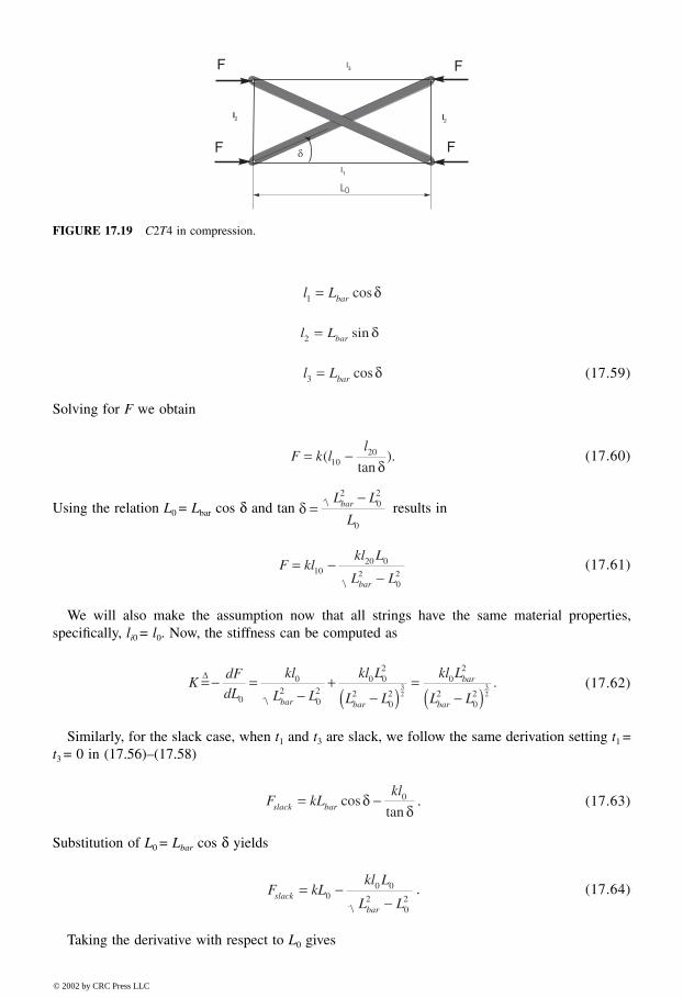
(17.59)

Solving for F we obtain

(17.60)

Using the relation L0 = Lbar cos δ and tan results in

(17.61)

We will also make the assumption now that all strings have the same material properties,specifically, li0 = l0. Now, the stiffness can be computed as

(17.62)

Similarly, for the slack case, when t1 and t3 are slack, we follow the same derivation setting t1 =t3 = 0 in (17.56)–(17.58)

. (17.63)

Substitution of L0 = Lbar cos δ yields

. (17.64)

Taking the derivative with respect to L0 gives

FIGURE 17.19 C2T4 in compression.

l Lbar1 = cosδ

l Lbar2 = sin δ

l Lbar3 = cosδ

F k ll

= −(tan

).1020

δ

δ =−L L

Lbar2

02

0

F klkl L

L Lbar

= −−10

20 0

202

KdFdL

kl

L L

kl L

L L

kl L

L Lbar bar

bar

bar

= − =−

+−( )

=−( )

∆

0

02

02

0 02

202

02

202

32

32

.

F kLkl

slack bar= −costan

δδ

0

F kLkl L

L Lslack

bar

= −−0

0 0

202



. (17.65)

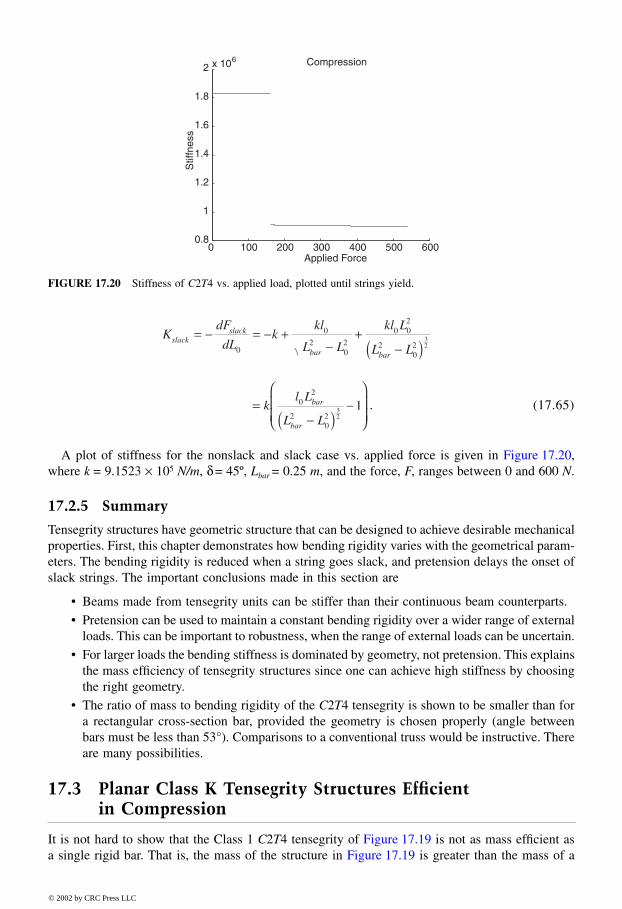
A plot of stiffness for the nonslack and slack case vs. applied force is given in Figure 17.20,where k = 9.1523 × 105 N/m, δ = 45º, Lbar = 0.25 m, and the force, F, ranges between 0 and 600 N.

17.2.5 Summary

Tensegrity structures have geometric structure that can be designed to achieve desirable mechanicalproperties. First, this chapter demonstrates how bending rigidity varies with the geometrical param-eters. The bending rigidity is reduced when a string goes slack, and pretension delays the onset ofslack strings. The important conclusions made in this section are

• Beams made from tensegrity units can be stiffer than their continuous beam counterparts.

• Pretension can be used to maintain a constant bending rigidity over a wider range of externalloads. This can be important to robustness, when the range of external loads can be uncertain.

• For larger loads the bending stiffness is dominated by geometry, not pretension. This explainsthe mass efficiency of tensegrity structures since one can achieve high stiffness by choosingthe right geometry.

• The ratio of mass to bending rigidity of the C2T4 tensegrity is shown to be smaller than fora rectangular cross-section bar, provided the geometry is chosen properly (angle betweenbars must be less than 53°). Comparisons to a conventional truss would be instructive. Thereare many possibilities.

17.3 Planar Class K Tensegrity Structures Efficient in Compression

It is not hard to show that the Class 1 C2T4 tensegrity of Figure 17.19 is not as mass efficient asa single rigid bar. That is, the mass of the structure in Figure 17.19 is greater than the mass of a

FIGURE 17.20 Stiffness of C2T4 vs. applied load, plotted until strings yield.

0 100 200 300 400 500 6000.8

1

1.2

1.4

1.6

1.8

2 x 106

Applied Force

Stif

fnes

s

Compression

KdF

dLk

kl

L L

kl L

L Lslack

slack

bar bar

= − = − +−

+−( )0

0

202

0 02

202

32

=−( )

−

kl L

L L

bar

bar

02

202

32

1



single bar which buckles at the same load 2F. This motivates the examination of Class 2 tensegritystructures which have the potential of greater strength and stiffness due to ball joints that canefficiently transfer loads from one bar to another. Compressive members are disconnected in thetraditional definition2 of tensegrity structures, which we call Class 1 tensegrity. However, if stifftendons connecting two nodes are very short, then for all practical purposes, the nodes behave asthough they are connected. Hence, Class 1 tensegrity generates Class k tensegrity structures asspecial cases when certain tendons become relatively short. Class k tensegrity describes a networkof axially loaded members in which the ends of not more than k compressive members are connected(by ball joints, of course, because torques are not permitted) at nodes of the network.

In this section, we examine one basic structure that is efficient under compressive loads. In orderto design a structure that can carry a compressive load with small mass we employ Class k tensegritytogether with the concept of self-similarity. Self-similar structures involve replacing a compressivemember with a more efficient compressive system. This algorithm, or fractal, can be repeated foreach member in the structure. The basic principle responsible for the compression efficiency ofthis structure is geometrical advantage, combined with the use of tensile members that have beenshown to exhibit large load to mass ratios. We begin the derivation by starting with a single barand its Euler buckling conditions. Then this bar is replaced by four smaller bars and one tensilemember. This process can be generalized and the formulae are given in the following sections. Theobjective is to characterize the mass of the structure in terms of strength and stiffness. This allowsone to design for minimal mass while bounding stiffness. In designing this structure there are trade-offs; for example, geometrical complexity poses manufacturing difficulties.

The materials of the bars and strings used for all calculations in this section are steel, which hasthe mass density ρ = 7.862 , Young’s modulus E = 2.0611 and yield strength σ = 6.98

. Except when specified, we will normalize the length of the structures L0 = 1 in numericalcalculations.

17.3.1 Compressive Properties of the C4T2 Class 2 Tensegrity

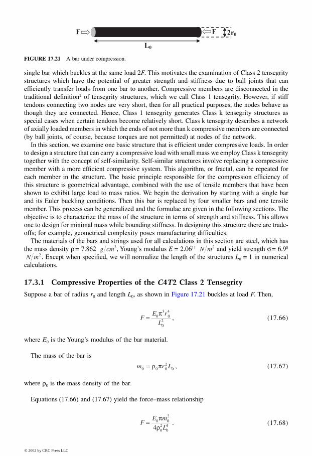
Suppose a bar of radius r0 and length L0, as shown in Figure 17.21 buckles at load F. Then,

, (17.66)

where E0 is the Young’s modulus of the bar material.

The mass of the bar is

, (17.67)

where ρ0 is the mass density of the bar.

Equations (17.66) and (17.67) yield the force–mass relationship

. (17.68)

FIGURE 17.21 A bar under compression.

g cm3 N m2

N m2

FE r

L= 0

304

02

π

m r L0 0 02

0= ρ π

FE m

L= 0 0

2

02

044

πρ



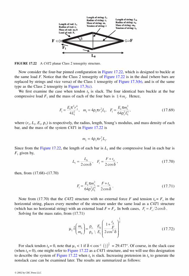
Now consider the four-bar pinned configuration in Figure 17.22, which is designed to buckle atthe same load F. Notice that the Class 2 tensegrity of Figure 17.22 is in the dual (where bars arereplaced by strings and vice versa) of the Class 1 tensegrity of Figure 17.3(b), and is of the sametype as the Class 2 tensegrity in Figure 17.3(c).

We first examine the case when tendon th is slack. The four identical bars buckle at the barcompressive load F1 and the mass of each of the four bars is Hence,

(17.69)

where (r1, L1, E1, ρ1) is respectively, the radius, length, Young’s modulus, and mass density of eachbar, and the mass of the system C4T1 in Figure 17.22 is

Since from the Figure 17.22, the length of each bar is L1 and the compressive load in each bar isF1 given by,

, (17.70)

then, from (17.68)–(17.70)

. (17.71)

Note from (17.70) that the C4T2 structure with no external force F and tension th = Fx in thehorizontal string, places every member of the structure under the same load as a C4T1 structure(which has no horizontal string) with an external load F = Fx. In both cases, .

Solving for the mass ratio, from (17.71)

(17.72)

For slack tendon th = 0, note that µ1 < 1 if δ < cos–1 = 29.477°. Of course, in the slack case(when th = 0), one might refer to Figure 17.22 as a C4T1 structure, and we will use this designationto describe the system of Figure 17.22 when th is slack. Increasing pretension in th to generate thenonslack case can be examined later. The results are summarized as follows:

FIGURE 17.22 A C4T2 planar Class 2 tensegrity structure.

1 4 1m .

FE r

Lm r L F

E m

L11

214

12 1 1 1

21 1

1 12

12

144

464

= = =π ρ π πρ

, , ,

m r L1 1 12

14= ρ π .

LL

FF th

10

12 2= =

+cos

,cosδ δ

FE m

L

F th1

1 12

12

1464 2

= =+π

ρ δcos

F Fx1 2= cosδ

µ ρρ δ1

1

0

1

0

0

15

12

1

2=

=+

∆ m

m

E

E

t

Fh

cos

12

15( )



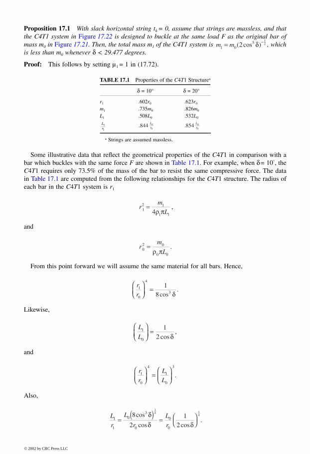
Proposition 17.1 With slack horizontal string th = 0, assume that strings are massless, and thatthe C4T1 system in Figure 17.22 is designed to buckle at the same load F as the original bar ofmass m0 in Figure 17.21. Then, the total mass m1 of the C4T1 system is , whichis less than m0 whenever δ < 29.477 degrees.

Proof: This follows by setting µ1 = 1 in (17.72).

Some illustrative data that reflect the geometrical properties of the C4T1 in comparison with abar which buckles with the same force F are shown in Table 17.1. For example, when δ = 10°, theC4T1 requires only 73.5% of the mass of the bar to resist the same compressive force. The datain Table 17.1 are computed from the following relationships for the C4T1 structure. The radius ofeach bar in the C4T1 system is r1

,

and

From this point forward we will assume the same material for all bars. Hence,

Likewise,

and

Also,

TABLE 17.1 Properties of the C4T1 Structurea

δ = 10° δ = 20°

r1 .602r0 .623r0

m1 .735m0 .826m0

L1 .508L0 .532L0

a Strings are assumed massless.

m m1 052

12= −( cos )δ

Lr1

1.844 0

0

Lr .854 0

0

Lr

rm

L12 1

1 14=

ρ π

rm

L02 0

0 0

=ρ π

.

r

r1

0

4

3

18

=

cos.

δ

L

L1

0

12

=

cos,

δ

r

r

L

L1

0

4

1

0

3

=

.

L

r

L

r

L

r1

1

03

0

0

0

8

21

2

14 1

4

=( )

=

cos

cos cos.

δδ δ



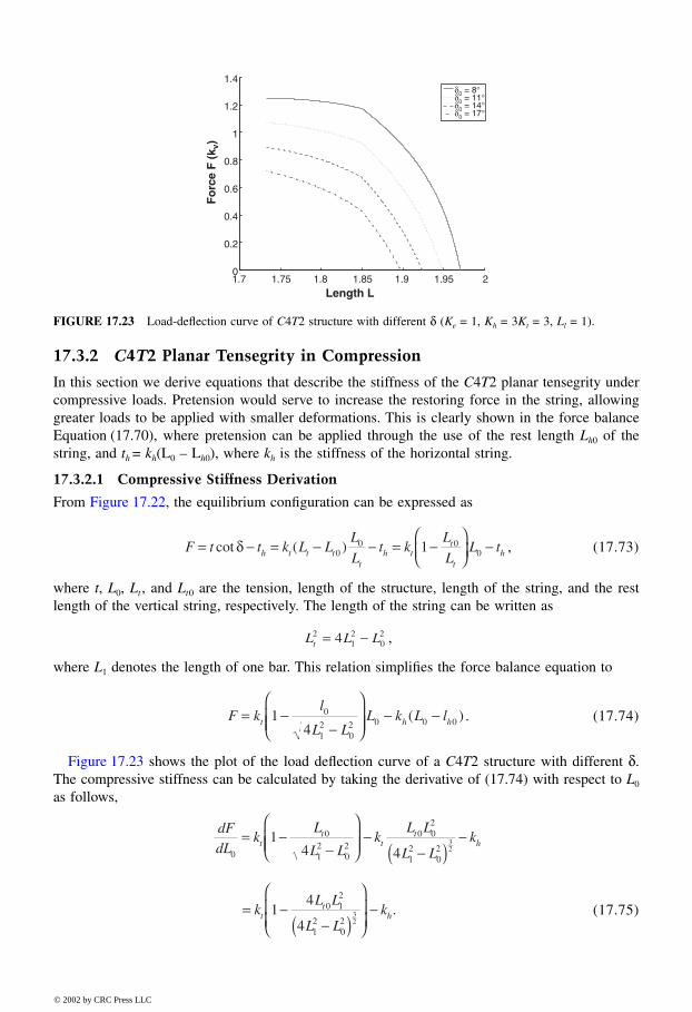
17.3.2 C4T2 Planar Tensegrity in Compression

In this section we derive equations that describe the stiffness of the C4T2 planar tensegrity undercompressive loads. Pretension would serve to increase the restoring force in the string, allowinggreater loads to be applied with smaller deformations. This is clearly shown in the force balanceEquation (17.70), where pretension can be applied through the use of the rest length Lh0 of thestring, and th = kh(L0 – Lh0), where kh is the stiffness of the horizontal string.

17.3.2.1 Compressive Stiffness Derivation

From Figure 17.22, the equilibrium configuration can be expressed as

, (17.73)

where t, L0, Lt , and Lt0 are the tension, length of the structure, length of the string, and the restlength of the vertical string, respectively. The length of the string can be written as

,

where L1 denotes the length of one bar. This relation simplifies the force balance equation to

. (17.74)

Figure 17.23 shows the plot of the load deflection curve of a C4T2 structure with different δ.The compressive stiffness can be calculated by taking the derivative of (17.74) with respect to L0

as follows,

(17.75)

FIGURE 17.23 Load-deflection curve of C4T2 structure with different δ (Ke = 1, Kh = 3Kt = 3, Ll = 1).

1.7 1.75 1.8 1.85 1.9 1.95 20

0.2

0.4

0.6

0.8

1

1.2

1.4

Length L

Fo

rce

F (

k v)

δ0 = 8°δ0 = 11°δ0 = 14°δ0 = 17°

F t t k L LL

Lt k

L

LL th t t t

th t

t

th= − = − − = −

−cot ( )δ 00 0

01

L L Lt2

12

024= −

F kl

L LL k L lt h h= −

−

− −1

40

12

02 0 0 0( )

dFdL

kL

L Lk

L L

L Lkt

tt

th

0

0

12

02

0 02

12

02

14 4

32

= −−

−

−( )−

= −−( )

−kL L

L Lkt

th1

4

4

0 12

12

02

32

.



Therefore, the stiffness is defined as

. (17.76)

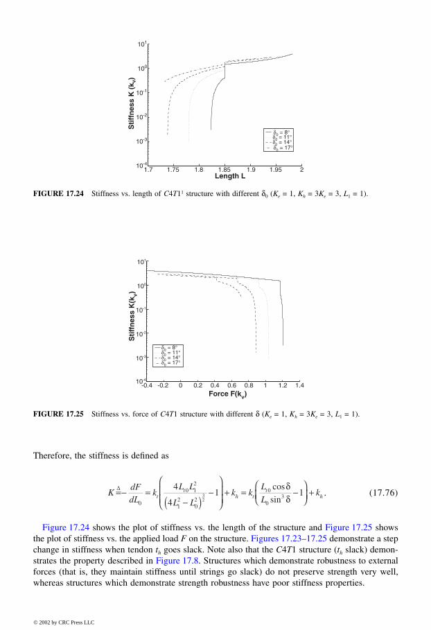
Figure 17.24 shows the plot of stiffness vs. the length of the structure and Figure 17.25 showsthe plot of stiffness vs. the applied load F on the structure. Figures 17.23–17.25 demonstrate a stepchange in stiffness when tendon th goes slack. Note also that the C4T1 structure (th slack) demon-strates the property described in Figure 17.8. Structures which demonstrate robustness to externalforces (that is, they maintain stiffness until strings go slack) do not preserve strength very well,whereas structures which demonstrate strength robustness have poor stiffness properties.

FIGURE 17.24 Stiffness vs. length of C4T11 structure with different δ0 (Ke = 1, Kh = 3Ke = 3, L1 = 1).

FIGURE 17.25 Stiffness vs. force of C4T1 structure with different δ (Ke = 1, Kh = 3Ke = 3, L1 = 1).

1.7 1.75 1.8 1.85 1.9 1.95 210-4

10-3

10-2

10-1

100

101

Length L

Sti

ffn

ess

K (

k v)

δ0 = 8°

δ0 = 11°δ0 = 14°δ0 = 17°

-0.4 -0.2 0 0.2 0.4 0.6 0.8 1 1.2 1.410-4

10-3

10-2

10-1

100

101

Force F(kv)

Sti

ffn

ess

K(k

v)

δ0 = 8°

δ0 = 11°δ0 = 14°δ0 = 17°

KdFdL

kL L

L Lk k

L

Lkt

th t

th=− =

−( )−

+ = −

+∆

0

0 12

12

02

0

03

4

41 13

2

cos

sin

δδ



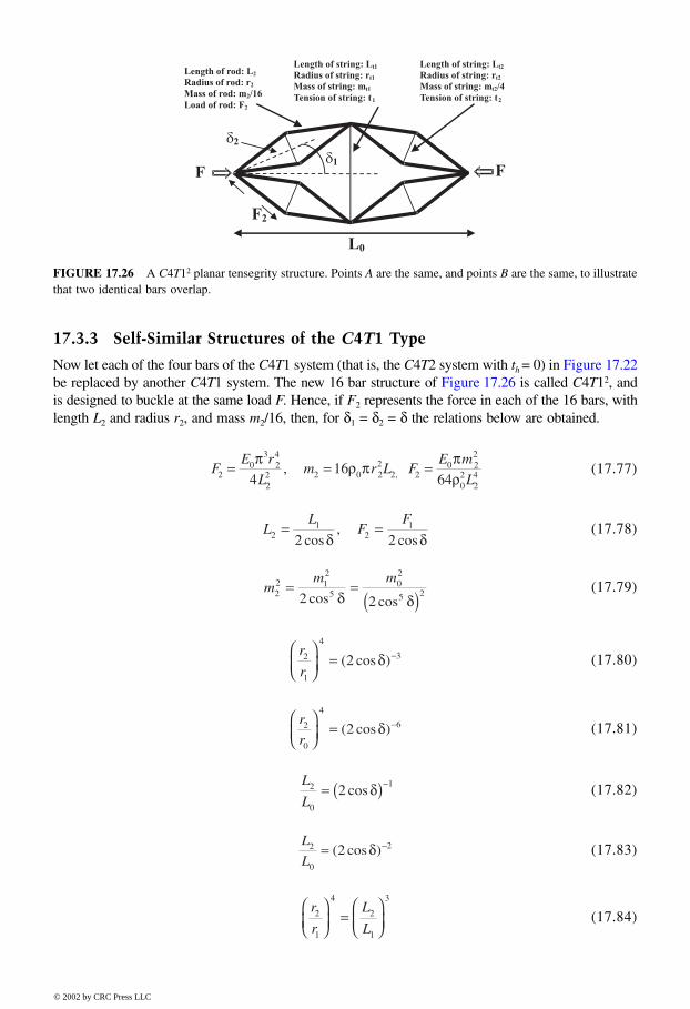
17.3.3 Self-Similar Structures of the C4T1 Type

Now let each of the four bars of the C4T1 system (that is, the C4T2 system with th = 0) in Figure 17.22be replaced by another C4T1 system. The new 16 bar structure of Figure 17.26 is called C4T12, andis designed to buckle at the same load F. Hence, if F2 represents the force in each of the 16 bars, withlength L2 and radius r2, and mass m2/16, then, for δ1 = δ2 = δ the relations below are obtained.

(17.77)

(17.78)

(17.79)

(17.80)

(17.81)

(17.82)

(17.83)

(17.84)

FIGURE 17.26 A C4T12 planar tensegrity structure. Points A are the same, and points B are the same, to illustratethat two identical bars overlap.

FE r

Lm r L F

E m

L20

324

22 2 0 2

22 2

0 22

02

244

1664

= = =π

ρ ππρ

, ,

LL

FF

21

21

2 2= =

cos,

cosδ δ

mm m

22 1

2

502

5 22 2= =

( )cos cosδ δ

r

r2

1

4

32

= −( cos )δ

r

r2

0

4

62

= −( cos )δ

L

L2

0

12= ( )−

cosδ

L

L2

0

22= −( cos )δ

r

r

L

L2

1

4

2

1

3

=

8596Ch17Frame 7 Friday, November 9, 2001 6:33 PM


(17.85)

(17.86)

Now let us replace each bar in the structure of Figure 17.26 by yet another C4T1 structure andcontinue this process indefinitely. To simplify the language for these instructions, we coin somenames that will simplify the description of the process we consider later.

Definition 17.3 Let the operation which replaces the bar of length L0 with the design ofFigure 17.22 be called the “C4T1 operator.” This replaces one compressive member with fourcompressive members plus one tension member, where the bar radii obey (17.88). Let δ be thesame for any i. Let the operation which replaces the design of the bar Figure 17.21 with the designof Figure 17.26 be called the “C4T12 operator.” If this C4T1 operation is repeated i times, thencall it the C4T1i operator, yielding the C4T1i system.

Lemma 17.2 Let the C4T1i operator be applied to the initial bar, always using the same materialand preserving buckling strength. Then, δ1 = δ the mass mi, bar radius ri , bar length Li of theC4T1i system satisfy:

(17.87)

(17.88)

(17.89)

(17.90)

(17.91)

. (17.92)

Note from (17.90) that the length-to-diameter ratio of the bars decreases with i if δ < 60°.Figure 17.27 illustrates C4T1i structures for i = 3, 4, 5, 6. Taking the limit of (17.87) as i → ∞

proves the following:

Theorem 17.1 Suppose the compressive force which buckles a C4T1i system is a specified value,F. Then if δ < 29.477°, the total mass of the bars in the C4T1i system approaches zero as i → ∞.

Proof: Take i toward infinity in (17.87). ❏

r

r

L

L2

0

4

2

0

3

=

L

r

L

r

L

r2

2

1

1

0

0

2 214

12= =− −

( cos ) ( cos )δ δ

m

mi

i

0

52 2= −( cos )δ

r

r

L

Li i

i

0 0

234

34

= =

−

( cos )δ

L

Li i

0

2= −( cos )δ

L

r

L

ri

i

i

= −0

0

2 4( cos )δ

FE r

L

E m

Lii

i

ii

i

= =04

20

2

202 44

πρ

m r Lii

i i= 4 02ρ π



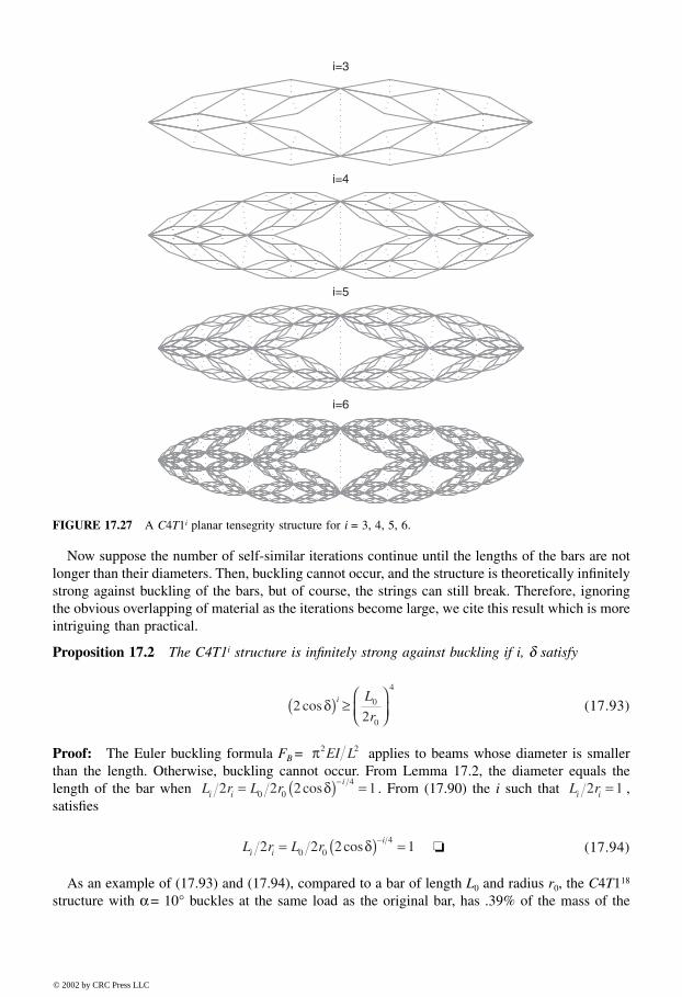
Now suppose the number of self-similar iterations continue until the lengths of the bars are notlonger than their diameters. Then, buckling cannot occur, and the structure is theoretically infinitelystrong against buckling of the bars, but of course, the strings can still break. Therefore, ignoringthe obvious overlapping of material as the iterations become large, we cite this result which is moreintriguing than practical.

Proposition 17.2 The C4T1i structure is infinitely strong against buckling if i, δ satisfy

(17.93)

Proof: The Euler buckling formula FB = applies to beams whose diameter is smallerthan the length. Otherwise, buckling cannot occur. From Lemma 17.2, the diameter equals thelength of the bar when . From (17.90) the i such that ,satisfies

❏ (17.94)

As an example of (17.93) and (17.94), compared to a bar of length L0 and radius r0, the C4T118

structure with α = 10° buckles at the same load as the original bar, has .39% of the mass of the

FIGURE 17.27 A C4T1i planar tensegrity structure for i = 3, 4, 5, 6.

i=3

i=4

i=5

i=6

22

0

0

4

cosδ( ) ≥

i L

r

π2 2EI L

L r L ri i

i2 2 2 10 0

4= ( ) =−cosδ L ri i2 1=

L r L ri i

i2 2 2 10 0

4= ( ) =−cosδ



original bar, and is infinitely stronger than the bar. For a given specified strength, this examplesuggests that solid materials are quite wasteful of mass. Of course, the above result has ignoredthe fact that the material overlaps, if one tried to place all elements in the same plane. However,multiple planar layers of elements can be pinned to give the desired planar effect mathematicallydescribed herein. A more important omission of the above analysis is the calculation of string mass.The string mass increases with self-similar iterations (increases with i) because strings are addedin the process. The mass of the bars decrease with i, so obviously minimal mass of the system(bars plus strings) occurs at finite i. This calculation will be shown momentarily.

17.3.3.1 Robustness of the C4T1

In this section we discuss briefly the issue of stability under a lateral force FL = 0 in Figure 17.22.We begin by mentioning two disastrous circumstances. First, if the applied force F is small and FL

is big, then the C4T1 will collapse. Second, if the angle δ is very small and F is big, then a modestlateral force FL will collapse the structure. Of course, a larger pretension in th will protect againstlarger FL. Three important points on more general structures of this type: first, big F always helpslateral robustness; second, larger δ helps lateral robustness; third, increasing th helps robustness.

17.3.3.2 Mass and Tension of String in a C4T11 Structure

The mass mt1, length Lt1 and tension t1 of string in the C4T11 structure are expressed as

(17.95)

(17.96)

and

, (17.97)

respectively.With (17.95) and (17.97),

Hence,

So, the mass of string mt1 is

(17.98)

m L rt t t t1 1 1 12= ρ π ,

L Lt1 0= tan ,δ

t F rt t1 1 12= =tan δ σ π

t F rm

Lt t tt

t t1 1 1

21

1

1 1

= = =tan .δ σ π σρ

m L Ftt

tt1

1

11= ρ

σδtan

=

ρσ

δπ

ρδt

tL

E m

L11 40

0 02

02

04( tan ) tan

=

E

Lm

t

t02

1 03

1

02 0

2

4

π δσ

ρρ

tan

=

E

Lr L m

t

t02

1 03

1

02 0 0

20 04

π δσ

ρρ

ρ πtan

.

mE

lmt

t

t1

02 2

1 02

1

0016

=

π δσ

ρρ

tan.



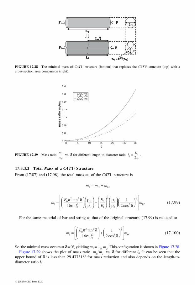
17.3.3.3 Total Mass of a C4T11 Structure

From (17.87) and (17.98), the total mass m1 of the C4T11 structure is

(17.99)

For the same material of bar and string as that of the original structure, (17.99) is reduced to

(17.100)

So, the minimal mass occurs at δ = 0º, yielding m1 = . This configuration is shown in Figure 17.28.Figure 17.29 shows the plot of mass ratio vs. δ for different l0. It can be seen that the

upper bound of δ is less than 29.477318º for mass reduction and also depends on the length-to-diameter ratio l0.

FIGURE 17.28 The minimal mass of C4T11 structure (bottom) that replaces the C4T10 structure (top) with across-section area comparison (right).

FIGURE 17.29 Mass ratio vs. δ for different length-to-diameter ratio .

0 5 10 15 20 25 300.7

0.8

0.9

1

1.1

1.2

1.3

1.4

δ

mas

s ra

tio

m1/

m0

L0/2r0 =15L0/2r0 =30 L0/2r0 =45

m

m1

0

lL

ro0

0

2=

m m mt b1 1 1= +

mE

l

E

Em

t

t

o1

02 2

1 02

1 0

1

1

05 016

12

12 1

2

=

+

π δσ

ρρ

ρρ δ

tan

cos.

mE

lm

t1

02 2

1 02 5 016

12

12

=

+

π δσ δtan

cos.

12

mo

m m1 0



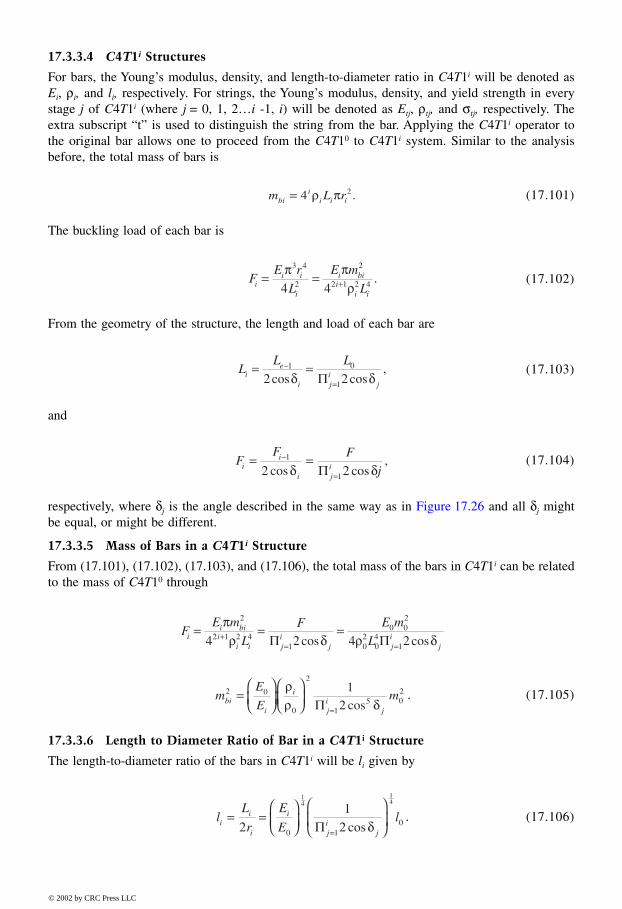
17.3.3.4 C4T1i Structures

For bars, the Young’s modulus, density, and length-to-diameter ratio in C4T1i will be denoted asEi, ρi, and li, respectively. For strings, the Young’s modulus, density, and yield strength in everystage j of C4T1i (where j = 0, 1, 2…i -1, i) will be denoted as Etj, ρtj, and σtj, respectively. Theextra subscript “t” is used to distinguish the string from the bar. Applying the C4T1i operator tothe original bar allows one to proceed from the C4T10 to C4T1i system. Similar to the analysisbefore, the total mass of bars is

(17.101)

The buckling load of each bar is

(17.102)

From the geometry of the structure, the length and load of each bar are

(17.103)

and

(17.104)

respectively, where δj is the angle described in the same way as in Figure 17.26 and all δj mightbe equal, or might be different.

17.3.3.5 Mass of Bars in a C4T1i Structure

From (17.101), (17.102), (17.103), and (17.106), the total mass of the bars in C4T1i can be relatedto the mass of C4T10 through

. (17.105)

17.3.3.6 Length to Diameter Ratio of Bar in a C4T1i Structure

The length-to-diameter ratio of the bars in C4T1i will be li given by

. (17.106)

m L rbii

i i i= 4 2ρ π .

FE r

L

E m

Lii i

i

i bii

i i

= = +π π

ρ

3 4

2

2

2 1 2 44 4.

LL L

ie

i ji

j

= =−

=

1 0

12 2cos cos,

δ δΠ

FF F

jii

i ji= =−

=

1

12 2cos cos,

δ δΠ

FE m

LF E m

Lii bi

ii i j

ij j

ij

= = =+= =

πρ δ ρ δ

2

2 1 2 41

0 02

02

04

14 2 4 2Π Πcos cos

mE

Embi

i

i

ji

j

2 0

0

2

15 0

212

=

=

ρρ δΠ cos

lL

r

E

Eli

i

i

i

ji

j

= =

=21

20 10

14

14

Π cosδ



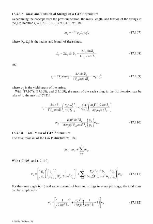
17.3.3.7 Mass and Tension of Strings in a C4T1i Structure

Generalizing the concept from the previous section, the mass, length, and tension of the strings inthe j-th iteration (j = 1,2,3,…i–1, i) of C4T1i will be

(17.107)

where (rtj, Ltj) is the radius and length of the strings,

(17.108)

and

(17.109)

where σtj is the yield stress of the string.With (17.107), (17.108), and (17.109), the mass of the each string in the i-th iteration can be

related to the mass of C4T10

. (17.110)

17.3.3.8 Total Mass of C4T1i Structure

The total mass mi of the C4T1i structure will be

With (17.105) and (17.110)

. (17.111)

For the same angle δj = δ and same material of bars and strings in every j-th stage, the total masscan be simplified to

(17.112)

m L rtjj

tj tj tj= −4 1 2ρ π ,

L LL

tj j jj

rj

r

= ==

22

20

1

sinsin

cos.δ

δδΠ

t FF

rj j jj

rj

jtj tj= = =

=

22

21

2sinsin

cos,δ

δδ

σ πΠ

tE m

L i

m

Ljj

rj

rtj

tj sj

s

tj j

=

=

=

=2

444

2

21

0 02

02

04

1

0

sin

cos

cos

sin

δδ

πρ

σδ

ρ δΠΠ

mE

lmtj

j

tj rj

r

tj=

=

02 2

02

12

0016

π δσ δ

ρρ

sin

cosΠ

m m mi bi tj

j

i

= +=

∑1

.

mE

E

E

lmi

i

i

ji

j

j

tj rj

j

tj

j

i

=

+

= ==

∑0

0 15

02 2

02

12

01

0

12

12

12 16

ρρ δ

π δσ δ

ρρΠ Πcos

sin

cos

mE

lmi

ti

i

=

+ −

12 16

115

02

02 2 0

2

cos cos.

δπ

σ δ



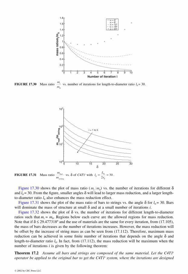
Figure 17.30 shows the plot of mass ratio ( ) vs. the number of iterations for different δand l0 = 30. From the figure, smaller angles δ will lead to larger mass reduction, and a larger length-to-diameter ratio l0 also enhances the mass reduction effect.

Figure 17.31 shows the plot of the mass ratio of bars to strings vs. the angle δ for l0 = 30. Barswill dominate the mass of structure at small δ and at a small number of iterations i.

Figure 17.32 shows the plot of δ vs. the number of iterations for different length-to-diameterratios such that mi = m0. Regions below each curve are the allowed regions for mass reduction.Note that if δ ≤ 29.477318º and the use of materials are the same for every iteration, from (17.105),the mass of bars decreases as the number of iterations increases. However, the mass reduction willbe offset by the increase of string mass as can be seen from (17.112). Therefore, maximum massreduction can be achieved in some finite number of iterations that depends on the angle δ andlength-to-diameter ratio l0. In fact, from (17.112), the mass reduction will be maximum when thenumber of iterations i is given by the following theorem:

Theorem 17.2 Assume all bars and strings are composed of the same material. Let the C4T1i

operator be applied to the original bar to get the C4T1i system, where the iterations are designed

FIGURE 17.30 Mass ratio vs. number of iterations for length-to-diameter ratio l0 = 30.

FIGURE 17.31 Mass ratio vs. δ of C4T1i with .

0 1 2 3 4 5 6 7 8 9 100

0.2

0.4

0.6

0.8

1

1.2

1.4

1.6

1.8

Number of iteration i

mas

s ra

tio

mi/m

0

α = 0°

α = 6°

α = 12°α = 18°α = 24°

m

mi

0

5 10 15 20 25 30100

101

102

103

δ

mro

d/m

stri

ng i = 1 to 5

m

mbar

string

lL

r00

0230= =

m mi 0



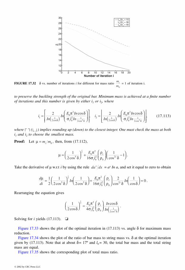
to preserve the buckling strength of the original bar. Minimum mass is achieved at a finite numberof iterations and this number is given by either i1 or i2, where

(17.113)

where ( ) implies rounding up (down) to the closest integer. One must check the mass at bothi1 and i2 to choose the smallest mass.

Proof: Let then, from (17.112),

.

Take the derivative of µ w.r.t i by using the rule = ax In a, and set it equal to zero to obtain

.

Rearranging the equation gives

.

Solving for i yields (17.113). ❏

Figure 17.33 shows the plot of the optimal iteration in (17.113) vs. angle δ for maximum massreduction.

Figure 17.34 shows the plot of the ratio of bar mass to string mass vs. δ at the optimal iterationgiven by (17.113). Note that at about δ = 17º and l0 = 30, the total bar mass and the total stringmass are equal.

Figure 17.35 shows the corresponding plot of total mass ratio.

FIGURE 17.32 δ vs. number of iterations i for different for mass ratio = 1 of iteration i.

0 2 4 6 8 10 12 14 16 18 2010

12

14

16

18

20

22

24

26

28

30

Number of iteration i

δ

L0/2r0 = 15L0/2r0 = 30L0/2r0 = 45

m

mi

0

iIn

InE In

l Ini

InIn

E In

l Int t1 1

2

02

02 1

2

2 12

02

02 1

2

2 2

5 5

= ( )

= ( )

cos cos cos cos

cos,

cos,

δ δ δ δ

π δσ

π δσ

µ = m mi 0 ,

µδ

πσ

ρρ δ

=

+

−

12 16

115

02

02

02

2

cos cos

i

E

lt

ti

da dxx

ddi

InE

lIn

i

t

ti

µδ δ

πσ

ρρ δ δ

=

+

=1

21

21

2 162 1

05 50

2

02

02

2

cos cos cos cos

12 4

12

5

02

02

01

2cos

cos

cosδ

πσ

ρρ

δ

δ

=

( )

E

lIn

Int

t



FIGURE 17.33 Optimal number of iterations i vs. δ for the maximum mass reduction.

FIGURE 17.34 Mass ratio of bars to strings vs. δ at the optimal iteration.

FIGURE 17.35 Total mass ratio vs. δ at the optimal iteration.

0 5 10 15 20 25 300

5

10

15

20

25

30

35

40

δ

nu

mb

er o

f it

erat

ion

i

L0/2r0 = 15L0/2r0 = 30L0/2r0 = 45

0 5 10 15 20 25

10-1

100

δ

mro

d/m

stri

ng

L0/2r0 = 10L0/2r0 = 20L0/2r0 = 30

m

mbar

string

0 5 10 15 20 25 300

0.1

0.2

0.3

0.4

0.5

0.6

0.7

0.8

0.9

1

δ

To

tal m

ass

rati

o m

i/m0

L0/2r0 = 10L0/2r0 = 20L0/2r0 = 30

m

mi

0



17.3.4 Stiffness of the C4T1i Structure

17.3.4.1 Stiffness Definition

For the C4T1i, the structure will change its length (measured from two nodal points where externalload is applied) in the same direction as the applied force. Therefore, the stiffness calculation is aone-dimensional problem. For an external load F applied to the structure of length L, the stiffnessK of the structure is defined as

, (17.114)

where the negative sign means the length of the structure decreases as the applied load increases.Since the external load can be related to the potential energy of the structure U by

,

the stiffness can also be calculated from the potential energy by

. (17.115)

17.3.4.2 The Stiffness Equation of a C4T1i Structure

In the calculations of stiffness (see Appendix 17.C), it is assumed that the stiffness of bars kbi andstrings ktj, where 1 ≤ j ≤ i, is constant under deformation. This is not always a good assumption,but other string stiffness models, such as can be analyzed in a straightforward manner.If Li0 and Ltj0 are the rest lengths of bars in the i-th iteration and strings in the j-th iteration,respectively, the stiffness of C4T1i is given by

, (17.116)

where, in the buckling design (see Appendix 17.B)

KdF

dL= −

FdU

dL= −

Kd U

dL=

2

2

k EA L=

K kL

L

k

k

L

L

L

L

k

k

L

L

L

Li tt

t

i t

bi

i

i

i j

j

i

t

tj

tj

tjo

tj= −

+

+

−

=

−

∑110

1

1

0 0

2

1

1

1

0

2 1

1 4 4

L Li si

s0 12= =Π cosδ

L Ltj i j s ji

s= = +2 21sin cosδ δΠ

k

k

E

Et

tj

t tj

tj t

1 1

1

=σσ

k

k

E

l

E

Et

bi

t

t isi

s1 1

1 02

01162

12= ( )=

πσ

δΠ cos

L

L Etjo

tj

tj

tj

= −1σ



In particular, if the materials of the bars and strings used are the same as those of original structure(C4T10) and δj = δ, the stiffness equation will be simplified to

(17.117)

where

17.3.4.3 The Rigid Bar Case

If the bar has infinite rigidity (large compared to the stiffness of strings), this means

,

then, the stiffness equation becomes

, (17.118)

where

Figure 17.36 shows the plot of the stiffness Ki vs. δ for length-to-diameter ratio l0 = 30.

kE E L

ltt

t1

0 13

0

1 0416

=π

σ

L

L lio

isi

s= + ( )=116

202 1

12π δΠ cos .

K kE

k

k

L

L

L

L E

L

L

kE

k

k

L

L

L

L

i tt

t

i t

bi

i

i

i t

t

j tj

j

i

tt

t

i t

bi

i

i

i

= − +

+ −

= − +

−−

=

−

∑11

0 0

2 1

1

0

2

1

1

11

0 0

4 1 4

4

σ σ

σ

+ −

−

− −2 1

2

1

11

1σ

δt

tiE cos

L Lii

0 2= ( cos )δ

k

k

E

lt

bi

t

t

i1

2

0216

2 2= ( )πσ

δcos

kE E L

ltt

t1

03

0

0464

=π

σ

L

L li

i

i0

021

162 2= + ( )π δcos .

k

kti

bi

→ 0

K ki t

iE

i

t

t=−

−

1

2

21

cos

cos

δδ

σ

kE E L

ltt

t1

03

0

0464

=π

σ.



Figure 17.37 shows the plot of the stiffness ratio vs. δ for the infinite rigid bar C4T1i

structure. Note that the ratio is independent of l0.Because the stiffness reduces with each iteration i, it is of interest to know how many iterations

may be taken before the stiffness violates a desired lower bound K.

Proposition 17.3 Given δ and a desired lower bound stiffness K of C4T1i, that is, K ≤ Ki , thenumber of iterations i which achieves this stiffness requirement is bounded by

(17.119)

Proof: From (17.118),

Rearrange the inequality to expose cos2i δ on one side and then take the log of both sides to obtain(17.119) ❏

FIGURE 17.36 Stiffness Ki of C4T1i structure with rigid bars vs. δ for l0 = 30.

FIGURE 17.37 Stiffness ratio of C4T1i structure with rigid bars vs. δ.

5 10 15 20 25 30106

107

108

109

1010

δ

Sti

ffn

ess

to le

ng

th r

atio

Ki /

L0

i = 1 to 10

5 10 15 20 25 3010-2

10-1

100

101

102

103

δ

Sti

ffn

ess

rati

o K

i /k t1

i = 1 to10

K

kti

1

K ki i1

i

Kkt

tEt

Kkt≤

+

+log

log.

1

11

2

σ

δcos

K K

k

i

t

iE

i

t

t

≤

≤−

−

1

2

21

cos

cos.

δδ

σ



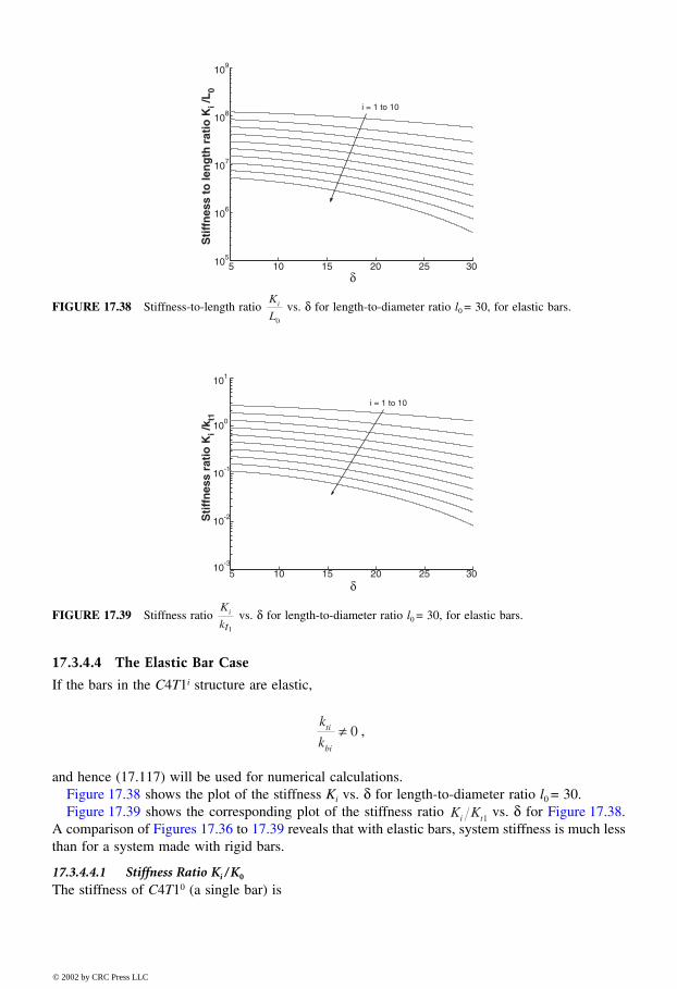
17.3.4.4 The Elastic Bar Case

If the bars in the C4T1i structure are elastic,

,

and hence (17.117) will be used for numerical calculations.Figure 17.38 shows the plot of the stiffness Ki vs. δ for length-to-diameter ratio l0 = 30.Figure 17.39 shows the corresponding plot of the stiffness ratio vs. δ for Figure 17.38.

A comparison of Figures 17.36 to 17.39 reveals that with elastic bars, system stiffness is much lessthan for a system made with rigid bars.

17.3.4.4.1 Stiffness Ratio Ki / K0

The stiffness of C4T10 (a single bar) is

FIGURE 17.38 Stiffness-to-length ratio vs. δ for length-to-diameter ratio l0 = 30, for elastic bars.

FIGURE 17.39 Stiffness ratio vs. δ for length-to-diameter ratio l0 = 30, for elastic bars.

5 10 15 20 25 30105

106

107

108

109

δ

Sti

ffn

ess

to le

ng

th r

atio

Ki /

L0

i = 1 to 10

K

Li

0

5 10 15 20 25 3010-3

10-2

10-1

100

101

δ

Sti

ffn

ess

rati

o K

i /k t1

i = 1 to 10

K

kti

1

k

kti

bi

≠ 0

K Ki t1



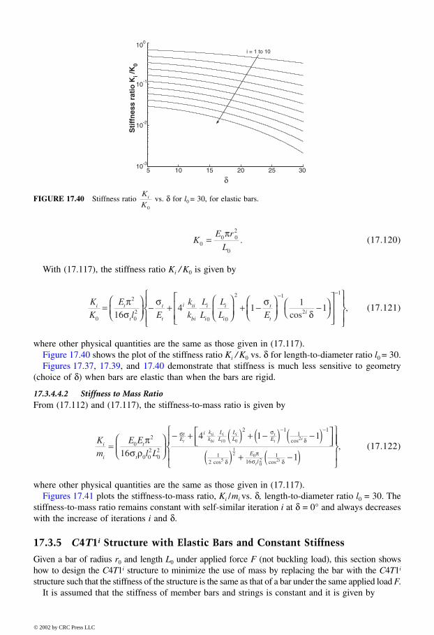
(17.120)

With (17.117), the stiffness ratio Ki / K0 is given by

(17.121)

where other physical quantities are the same as those given in (17.117).Figure 17.40 shows the plot of the stiffness ratio Ki / K0 vs. δ for length-to-diameter ratio l0 = 30.Figures 17.37, 17.39, and 17.40 demonstrate that stiffness is much less sensitive to geometry

(choice of δ) when bars are elastic than when the bars are rigid.

17.3.4.4.2 Stiffness to Mass RatioFrom (17.112) and (17.117), the stiffness-to-mass ratio is given by

(17.122)

where other physical quantities are the same as those given in (17.117).Figures 17.41 plots the stiffness-to-mass ratio, Ki /mi vs. δ, length-to-diameter ratio l0 = 30. The

stiffness-to-mass ratio remains constant with self-similar iteration i at δ = 0° and always decreaseswith the increase of iterations i and δ.

17.3.5 C4T1i Structure with Elastic Bars and Constant Stiffness

Given a bar of radius r0 and length L0 under applied force F (not buckling load), this section showshow to design the C4T1i structure to minimize the use of mass by replacing the bar with the C4T1i

structure such that the stiffness of the structure is the same as that of a bar under the same applied load F.It is assumed that the stiffness of member bars and strings is constant and it is given by

FIGURE 17.40 Stiffness ratio vs. δ for l0 = 30, for elastic bars.

5 10 15 20 25 3010-3

10-2

10-1

100

δ

Sti

ffn

ess

rati

o K

i /K

0

i = 1 to 10

K

Ki

0

KE r

L00 0

2

0

=π

.

K

K

E

l E

k

k

L

L

L

L Ei t

t

t

t

i ti

bi

i

i

i

i

t

ti

0

2

02

0 0

2 1

2

1

164 1

11=

− +

+ −

−

− −

πσ

σ σδcos

,

K

m

E E

l Li

i

t

t

tE

i kk

LL

LL E

E

l

t

ti

bi

i

i

i t

t i

t

=

− + ( ) + −( ) −( )

( ) + −( )

− −

02

0 02

02

2 11

1

12 16

116

4 1 1

1

0 0 2

12 0

20

πσ ρ

σ σδ

δπ

σ δ

cos

cos cos 5 2i

,



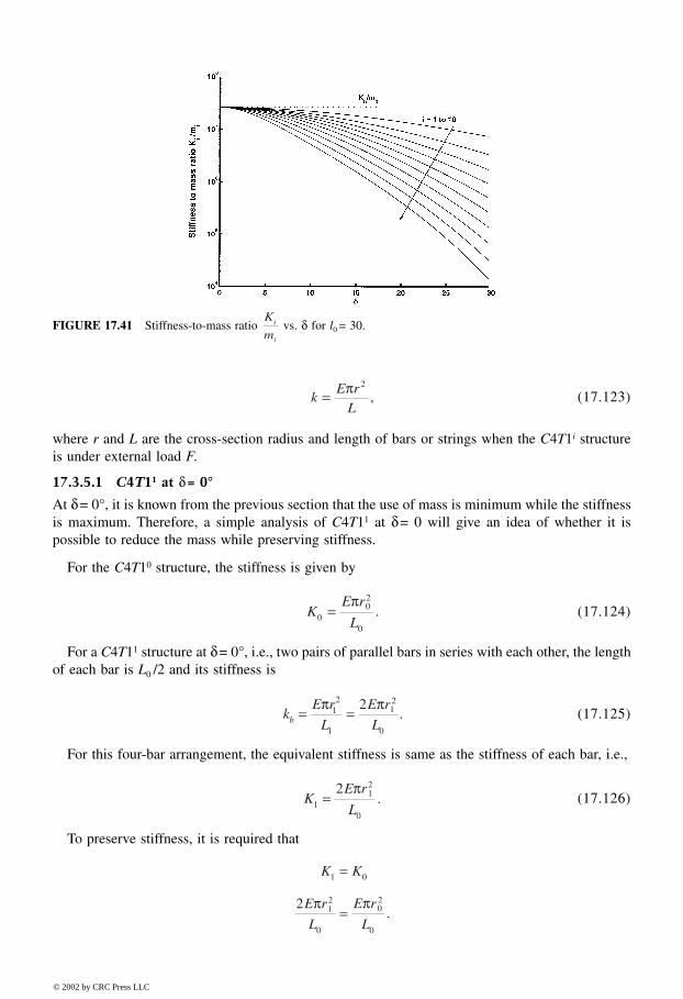
(17.123)

where r and L are the cross-section radius and length of bars or strings when the C4T1i structureis under external load F.

17.3.5.1 C4T11 at δ = 0°

At δ = 0°, it is known from the previous section that the use of mass is minimum while the stiffnessis maximum. Therefore, a simple analysis of C4T11 at δ = 0 will give an idea of whether it ispossible to reduce the mass while preserving stiffness.

For the C4T10 structure, the stiffness is given by

(17.124)

For a C4T11 structure at δ = 0°, i.e., two pairs of parallel bars in series with each other, the lengthof each bar is L0 /2 and its stiffness is

(17.125)

For this four-bar arrangement, the equivalent stiffness is same as the stiffness of each bar, i.e.,

(17.126)

To preserve stiffness, it is required that

FIGURE 17.41 Stiffness-to-mass ratio vs. δ for l0 = 30.K

mi

i

kE r

L= π 2

,

KE r

L002

0

=π

.

kE r

L

E r

Lb = =π π12

1

12

0

2.

KE r

L112

0

2=

π.

K K

E r

L

E r

L

1 0

12

0

02

0

2

=

=π π

.



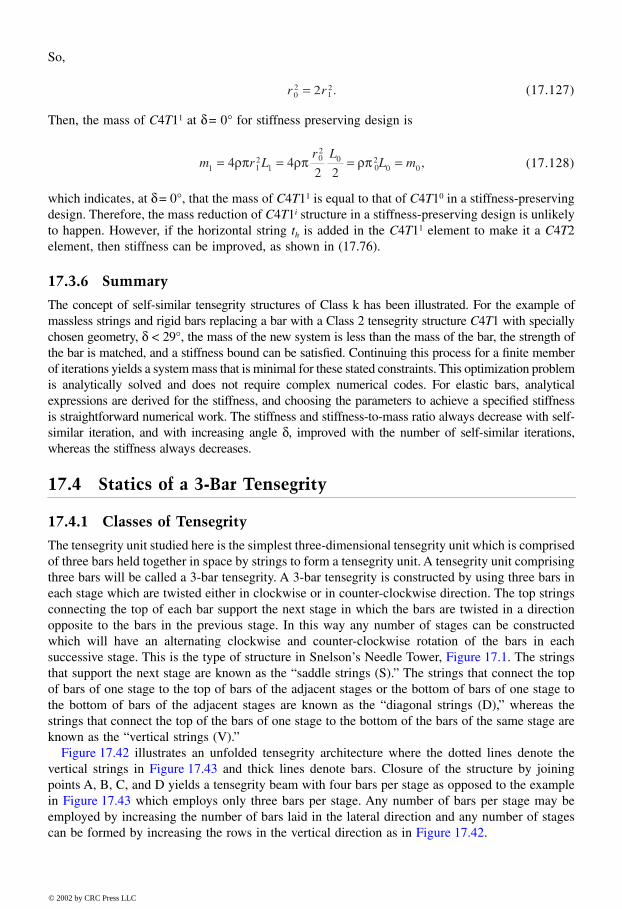
So,

(17.127)

Then, the mass of C4T11 at δ = 0° for stiffness preserving design is

(17.128)

which indicates, at δ = 0°, that the mass of C4T11 is equal to that of C4T10 in a stiffness-preservingdesign. Therefore, the mass reduction of C4T1i structure in a stiffness-preserving design is unlikelyto happen. However, if the horizontal string th is added in the C4T11 element to make it a C4T2element, then stiffness can be improved, as shown in (17.76).

17.3.6 Summary

The concept of self-similar tensegrity structures of Class k has been illustrated. For the example ofmassless strings and rigid bars replacing a bar with a Class 2 tensegrity structure C4T1 with speciallychosen geometry, δ < 29°, the mass of the new system is less than the mass of the bar, the strength ofthe bar is matched, and a stiffness bound can be satisfied. Continuing this process for a finite memberof iterations yields a system mass that is minimal for these stated constraints. This optimization problemis analytically solved and does not require complex numerical codes. For elastic bars, analyticalexpressions are derived for the stiffness, and choosing the parameters to achieve a specified stiffnessis straightforward numerical work. The stiffness and stiffness-to-mass ratio always decrease with self-similar iteration, and with increasing angle δ, improved with the number of self-similar iterations,whereas the stiffness always decreases.

17.4 Statics of a 3-Bar Tensegrity

17.4.1 Classes of Tensegrity

The tensegrity unit studied here is the simplest three-dimensional tensegrity unit which is comprisedof three bars held together in space by strings to form a tensegrity unit. A tensegrity unit comprisingthree bars will be called a 3-bar tensegrity. A 3-bar tensegrity is constructed by using three bars ineach stage which are twisted either in clockwise or in counter-clockwise direction. The top stringsconnecting the top of each bar support the next stage in which the bars are twisted in a directionopposite to the bars in the previous stage. In this way any number of stages can be constructedwhich will have an alternating clockwise and counter-clockwise rotation of the bars in eachsuccessive stage. This is the type of structure in Snelson’s Needle Tower, Figure 17.1. The stringsthat support the next stage are known as the “saddle strings (S).” The strings that connect the topof bars of one stage to the top of bars of the adjacent stages or the bottom of bars of one stage tothe bottom of bars of the adjacent stages are known as the “diagonal strings (D),” whereas thestrings that connect the top of the bars of one stage to the bottom of the bars of the same stage areknown as the “vertical strings (V).”

Figure 17.42 illustrates an unfolded tensegrity architecture where the dotted lines denote thevertical strings in Figure 17.43 and thick lines denote bars. Closure of the structure by joiningpoints A, B, C, and D yields a tensegrity beam with four bars per stage as opposed to the examplein Figure 17.43 which employs only three bars per stage. Any number of bars per stage may beemployed by increasing the number of bars laid in the lateral direction and any number of stagescan be formed by increasing the rows in the vertical direction as in Figure 17.42.

r r02

122= .

m r Lr L

L m1 12

102

002

0 04 42 2

= = = =ρπ ρπ ρπ ,



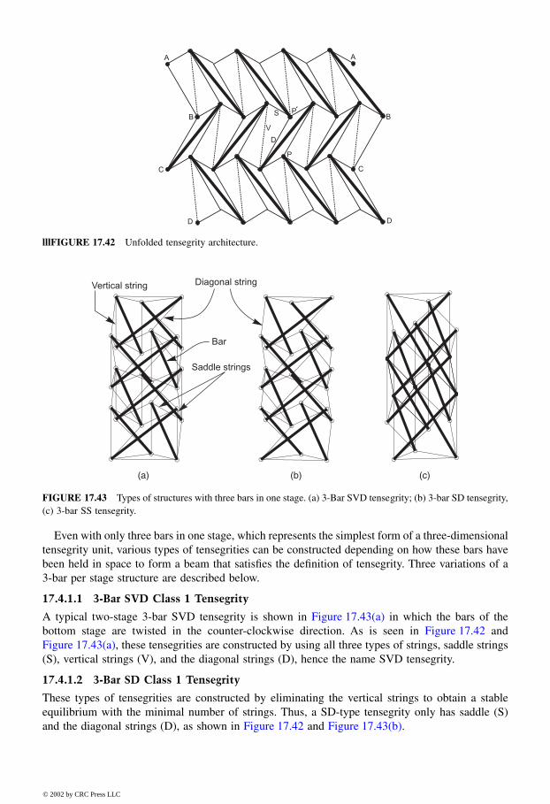
Even with only three bars in one stage, which represents the simplest form of a three-dimensionaltensegrity unit, various types of tensegrities can be constructed depending on how these bars havebeen held in space to form a beam that satisfies the definition of tensegrity. Three variations of a3-bar per stage structure are described below.

17.4.1.1 3-Bar SVD Class 1 Tensegrity

A typical two-stage 3-bar SVD tensegrity is shown in Figure 17.43(a) in which the bars of thebottom stage are twisted in the counter-clockwise direction. As is seen in Figure 17.42 andFigure 17.43(a), these tensegrities are constructed by using all three types of strings, saddle strings(S), vertical strings (V), and the diagonal strings (D), hence the name SVD tensegrity.

17.4.1.2 3-Bar SD Class 1 Tensegrity

These types of tensegrities are constructed by eliminating the vertical strings to obtain a stableequilibrium with the minimal number of strings. Thus, a SD-type tensegrity only has saddle (S)and the diagonal strings (D), as shown in Figure 17.42 and Figure 17.43(b).

lllFIGURE 17.42 Unfolded tensegrity architecture.

FIGURE 17.43 Types of structures with three bars in one stage. (a) 3-Bar SVD tensegrity; (b) 3-bar SD tensegrity,(c) 3-bar SS tensegrity.

(a) (b) (c)



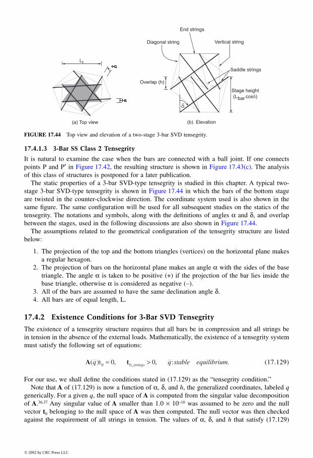
17.4.1.3 3-Bar SS Class 2 Tensegrity

It is natural to examine the case when the bars are connected with a ball joint. If one connectspoints P and P′ in Figure 17.42, the resulting structure is shown in Figure 17.43(c). The analysisof this class of structures is postponed for a later publication.

The static properties of a 3-bar SVD-type tensegrity is studied in this chapter. A typical two-stage 3-bar SVD-type tensegrity is shown in Figure 17.44 in which the bars of the bottom stageare twisted in the counter-clockwise direction. The coordinate system used is also shown in thesame figure. The same configuration will be used for all subsequent studies on the statics of thetensegrity. The notations and symbols, along with the definitions of angles α and δ, and overlapbetween the stages, used in the following discussions are also shown in Figure 17.44.

The assumptions related to the geometrical configuration of the tensegrity structure are listedbelow:

1. The projection of the top and the bottom triangles (vertices) on the horizontal plane makesa regular hexagon.

2. The projection of bars on the horizontal plane makes an angle α with the sides of the basetriangle. The angle α is taken to be positive (+) if the projection of the bar lies inside thebase triangle, otherwise α is considered as negative (–).

3. All of the bars are assumed to have the same declination angle δ.4. All bars are of equal length, L.

17.4.2 Existence Conditions for 3-Bar SVD Tensegrity

The existence of a tensegrity structure requires that all bars be in compression and all strings bein tension in the absence of the external loads. Mathematically, the existence of a tensegrity systemmust satisfy the following set of equations:

(17.129)

For our use, we shall define the conditions stated in (17.129) as the “tensegrity condition.”Note that A of (17.129) is now a function of α, δ, and h, the generalized coordinates, labeled q

generically. For a given q, the null space of A is computed from the singular value decompositionof A.36,37 Any singular value of A smaller than 1.0 × 10–10 was assumed to be zero and the nullvector t0 belonging to the null space of A was then computed. The null vector was then checkedagainst the requirement of all strings in tension. The values of α, δ, and h that satisfy (17.129)

FIGURE 17.44 Top view and elevation of a two-stage 3-bar SVD tensegrity.

A t( ) , , : .q q stable equilibriumstringst 0 0_= >0 0



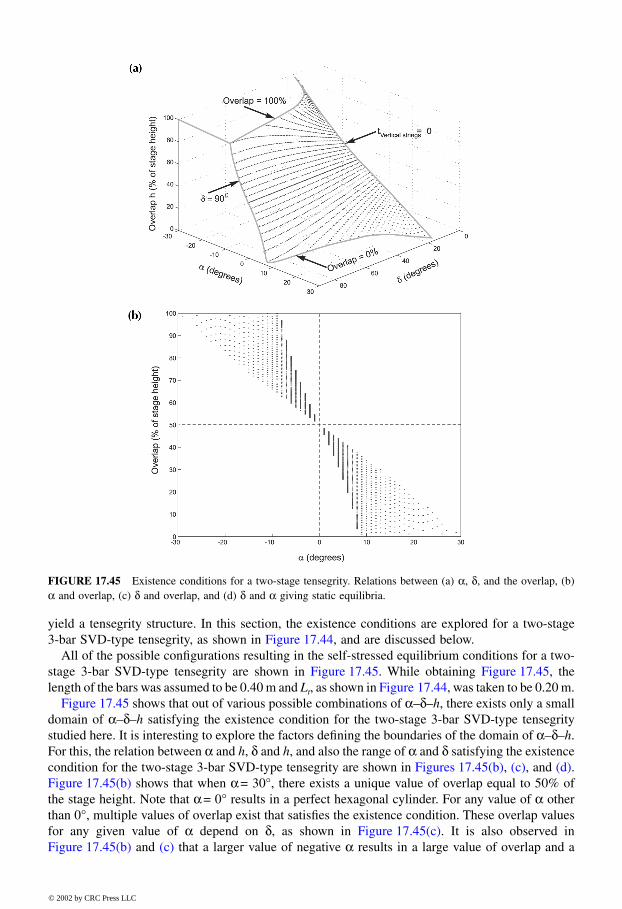
yield a tensegrity structure. In this section, the existence conditions are explored for a two-stage3-bar SVD-type tensegrity, as shown in Figure 17.44, and are discussed below.

All of the possible configurations resulting in the self-stressed equilibrium conditions for a two-stage 3-bar SVD-type tensegrity are shown in Figure 17.45. While obtaining Figure 17.45, thelength of the bars was assumed to be 0.40 m and Lt, as shown in Figure 17.44, was taken to be 0.20 m.

Figure 17.45 shows that out of various possible combinations of α–δ–h, there exists only a smalldomain of α–δ–h satisfying the existence condition for the two-stage 3-bar SVD-type tensegritystudied here. It is interesting to explore the factors defining the boundaries of the domain of α–δ–h.For this, the relation between α and h, δ and h, and also the range of α and δ satisfying the existencecondition for the two-stage 3-bar SVD-type tensegrity are shown in Figures 17.45(b), (c), and (d).Figure 17.45(b) shows that when α = 30°, there exists a unique value of overlap equal to 50% ofthe stage height. Note that α = 0° results in a perfect hexagonal cylinder. For any value of α otherthan 0°, multiple values of overlap exist that satisfies the existence condition. These overlap valuesfor any given value of α depend on δ, as shown in Figure 17.45(c). It is also observed inFigure 17.45(b) and (c) that a larger value of negative α results in a large value of overlap and a

FIGURE 17.45 Existence conditions for a two-stage tensegrity. Relations between (a) α, δ, and the overlap, (b)α and overlap, (c) δ and overlap, and (d) δ and α giving static equilibria.



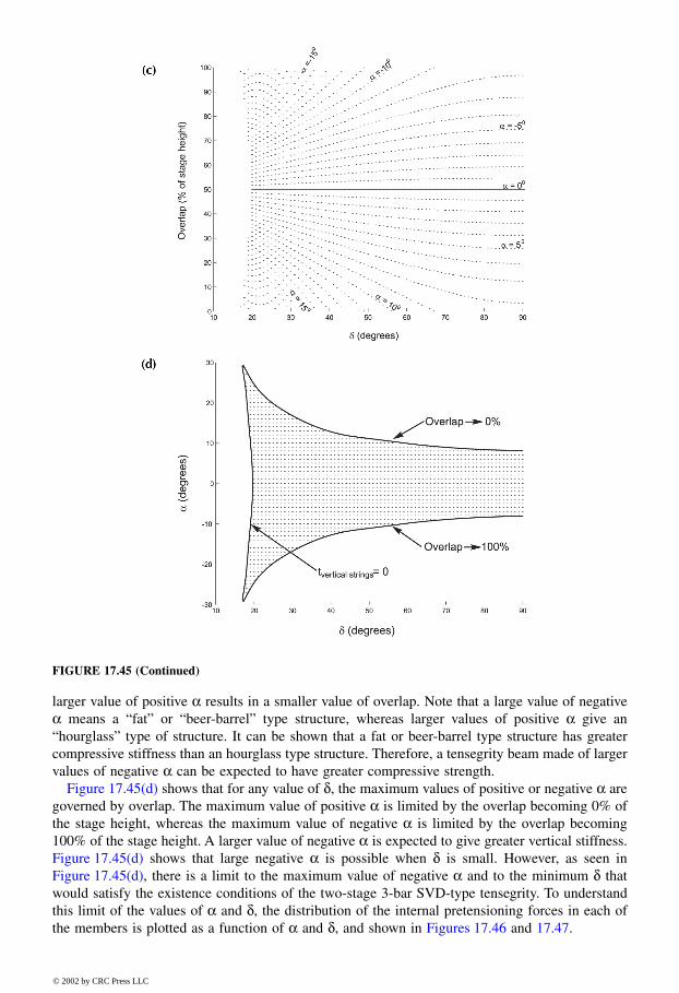
larger value of positive α results in a smaller value of overlap. Note that a large value of negativeα means a “fat” or “beer-barrel” type structure, whereas larger values of positive α give an“hourglass” type of structure. It can be shown that a fat or beer-barrel type structure has greatercompressive stiffness than an hourglass type structure. Therefore, a tensegrity beam made of largervalues of negative α can be expected to have greater compressive strength.

Figure 17.45(d) shows that for any value of δ, the maximum values of positive or negative α aregoverned by overlap. The maximum value of positive α is limited by the overlap becoming 0% ofthe stage height, whereas the maximum value of negative α is limited by the overlap becoming100% of the stage height. A larger value of negative α is expected to give greater vertical stiffness.Figure 17.45(d) shows that large negative α is possible when δ is small. However, as seen inFigure 17.45(d), there is a limit to the maximum value of negative α and to the minimum δ thatwould satisfy the existence conditions of the two-stage 3-bar SVD-type tensegrity. To understandthis limit of the values of α and δ, the distribution of the internal pretensioning forces in each ofthe members is plotted as a function of α and δ, and shown in Figures 17.46 and 17.47.

FIGURE 17.45 (Continued)


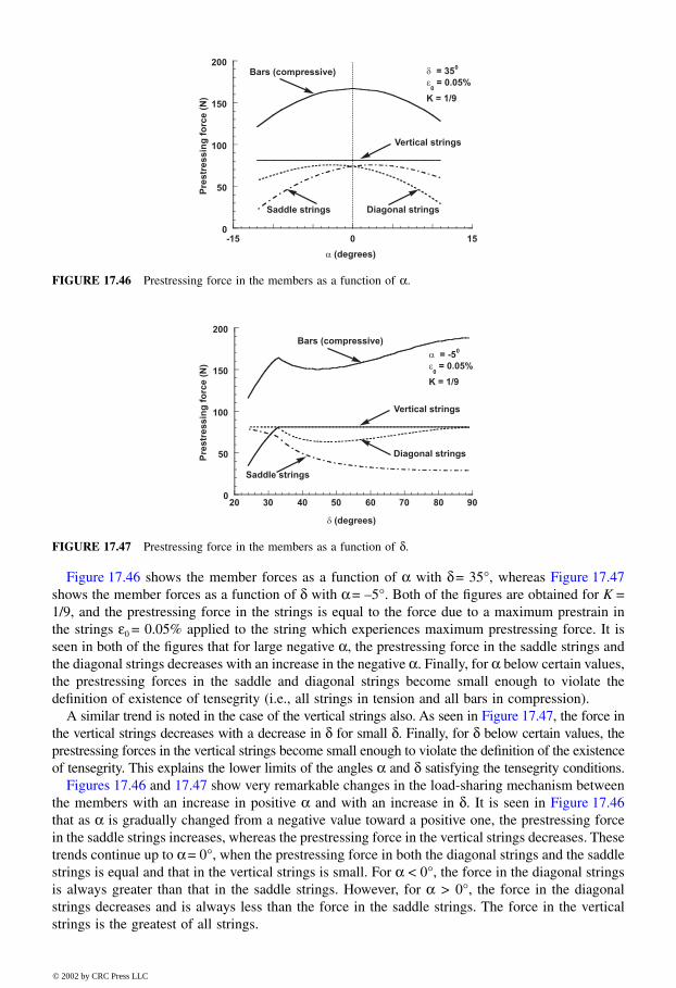
Figure 17.46 shows the member forces as a function of α with δ = 35°, whereas Figure 17.47shows the member forces as a function of δ with α = –5°. Both of the figures are obtained for K =1/9, and the prestressing force in the strings is equal to the force due to a maximum prestrain inthe strings ε0 = 0.05% applied to the string which experiences maximum prestressing force. It isseen in both of the figures that for large negative α, the prestressing force in the saddle strings andthe diagonal strings decreases with an increase in the negative α. Finally, for α below certain values,the prestressing forces in the saddle and diagonal strings become small enough to violate thedefinition of existence of tensegrity (i.e., all strings in tension and all bars in compression).

A similar trend is noted in the case of the vertical strings also. As seen in Figure 17.47, the force inthe vertical strings decreases with a decrease in δ for small δ. Finally, for δ below certain values, theprestressing forces in the vertical strings become small enough to violate the definition of the existenceof tensegrity. This explains the lower limits of the angles α and δ satisfying the tensegrity conditions.

Figures 17.46 and 17.47 show very remarkable changes in the load-sharing mechanism betweenthe members with an increase in positive α and with an increase in δ. It is seen in Figure 17.46that as α is gradually changed from a negative value toward a positive one, the prestressing forcein the saddle strings increases, whereas the prestressing force in the vertical strings decreases. Thesetrends continue up to α = 0°, when the prestressing force in both the diagonal strings and the saddlestrings is equal and that in the vertical strings is small. For α < 0°, the force in the diagonal stringsis always greater than that in the saddle strings. However, for α > 0°, the force in the diagonalstrings decreases and is always less than the force in the saddle strings. The force in the verticalstrings is the greatest of all strings.

FIGURE 17.46 Prestressing force in the members as a function of α.

FIGURE 17.47 Prestressing force in the members as a function of δ.



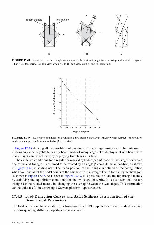
Figure 17.45 showing all the possible configurations of a two-stage tensegrity can be quite usefulin designing a deployable tensegrity beam made of many stages. The deployment of a beam withmany stages can be achieved by deploying two stages at a time.

The existence conditions for a regular hexagonal cylinder (beam) made of two stages for whichone of the end triangles is assumed to be rotated by an angle β about its mean position, as shownin Figure 17.48, is studied next. The mean position of the triangle is defined as the configurationwhen β = 0 and all of the nodal points of the bars line up in a straight line to form a regular hexagon,as shown in Figure 17.48. As is seen in Figure 17.49, it is possible to rotate the top triangle merelyby satisfying the equilibrium conditions for the two-stage tensegrity. It is also seen that the toptriangle can be rotated merely by changing the overlap between the two stages. This informationcan be quite useful in designing a Stewart platform-type structure.

17.4.3 Load-Deflection Curves and Axial Stiffness as a Function of the Geometrical Parameters

The load deflection characteristics of a two-stage 3-bar SVD-type tensegrity are studied next andthe corresponding stiffness properties are investigated.

FIGURE 17.48 Rotation of the top triangle with respect to the bottom triangle for a two-stage cylindrical hexagonal3-bar SVD tensegrity. (a) Top view when β = 0, (b) top view with β, and (c) elevation.

FIGURE 17.49 Existence conditions for a cylindrical two-stage 3-bars SVD tensegrity with respect to the rotationangle of the top triangle (anticlockwise β is positive).



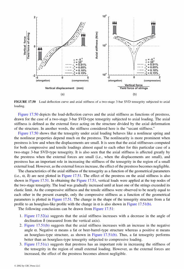
Figure 17.50 depicts the load-deflection curves and the axial stiffness as functions of prestress,drawn for the case of a two-stage 3-bar SVD-type tensegrity subjected to axial loading. The axialstiffness is defined as the external force acting on the structure divided by the axial deformationof the structure. In another words, the stiffness considered here is the “secant stiffness.”

Figure 17.50 shows that the tensegrity under axial loading behaves like a nonlinear spring andthe nonlinear properties depend much on the prestress. The nonlinearity is more prominent whenprestress is low and when the displacements are small. It is seen that the axial stiffnesses computedfor both compressive and tensile loadings almost equal to each other for this particular case of atwo-stage 3-bar SVD-type tensegrity. It is also seen that the axial stiffness is affected greatly bythe prestress when the external forces are small (i.e., when the displacements are small), andprestress has an important role in increasing the stiffness of the tensegrity in the region of a smallexternal load. However, as the external forces increase, the effect of the prestress becomes negligible.

The characteristics of the axial stiffness of the tensegrity as a function of the geometrical parameters(i.e., α, δ) are next plotted in Figure 17.51. The effect of the prestress on the axial stiffness is alsoshown in Figure 17.51. In obtaining the Figure 17.51, vertical loads were applied at the top nodes ofthe two-stage tensegrity. The load was gradually increased until at least one of the strings exceeded itselastic limit. As the compressive stiffness and the tensile stiffness were observed to be nearly equal toeach other in the present example, only the compressive stiffness as a function of the geometricalparameters is plotted in Figure 17.51. The change in the shape of the tensegrity structure from a fatprofile to an hourglass-like profile with the change in α is also shown in Figure 17.51(b).

The following conclusions can be drawn from Figure 17.51:

1. Figure 17.52(a) suggests that the axial stiffness increases with a decrease in the angle ofdeclination δ (measured from the vertical axis).

2. Figure 17.51(b) suggests that the axial stiffness increases with an increase in the negativeangle α. Negative α means a fat or beer-barrel-type structure whereas a positive α meansan hourglass-type structure, as shown in Figure 17.51(b). Thus, a fat tensegrity performsbetter than an hourglass-type tensegrity subjected to compressive loading.

3. Figure 17.51(c) suggests that prestress has an important role in increasing the stiffness ofthe tensegrity in the region of small external loading. However, as the external forces areincreased, the effect of the prestress becomes almost negligible.

FIGURE 17.50 Load deflection curve and axial stiffness of a two-stage 3-bar SVD tensegrity subjected to axialloading.

(a) (b)



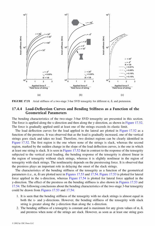
17.4.4 Load-Deflection Curves and Bending Stiffness as a Function of the Geometrical Parameters

The bending characteristics of the two-stage 3-bar SVD tensegrity are presented in this section.The force is applied along the x-direction and then along the y-direction, as shown in Figure 17.52.The force is gradually applied until at least one of the strings exceeds its elastic limit.

The load deflection curves for the load applied in the lateral are plotted in Figure 17.52 as afunction of the prestress. It was observed that as the load is gradually increased, one of the verticalstrings goes slack and takes no load. Therefore, two distinct regions can be clearly identified inFigure 17.52. The first region is the one where none of the strings is slack, whereas the secondregion, marked by the sudden change in the slope of the load deflection curves, is the one in whichat least one string is slack. It is seen in Figure 17.52 that in contrast to the response of the tensegritysubjected to the vertical axial loading, the bending response of the tensegrity is almost linear inthe region of tensegrity without slack strings, whereas it is slightly nonlinear in the region oftensegrity with slack strings. The nonlinearity depends on the prestressing force. It is observed thatthe prestress plays an important role in delaying the onset of the slack strings.

The characteristics of the bending stiffness of the tensegrity as a function of the geometricalparameters (i.e., α, δ) are plotted next in Figures 17.53 and 17.54. Figure 17.53 is plotted for lateralforce applied in the x-direction, whereas Figure 17.54 is plotted for lateral force applied in they-direction. The effect of the prestress on the bending stiffness is also shown in Figures 17.53 and17.54. The following conclusions about the bending characteristics of the two-stage 3-bar tensegritycould be drawn from Figures 17.53 and 17.54:

1. It is seen that the bending stiffness of the tensegrity with no slack strings is almost equal inboth the x- and y-directions. However, the bending stiffness of the tensegrity with slackstring is greater along the y-direction than along the x-direction.

2. The bending stiffness of a tensegrity is constant and is maximum for any given values of α, δ,and prestress when none of the strings are slack. However, as soon as at least one string goes

FIGURE 17.51 Axial stiffness of a two-stage 3-bar SVD tensegrity for different α, δ, and pretension.

(a) (b) (c)



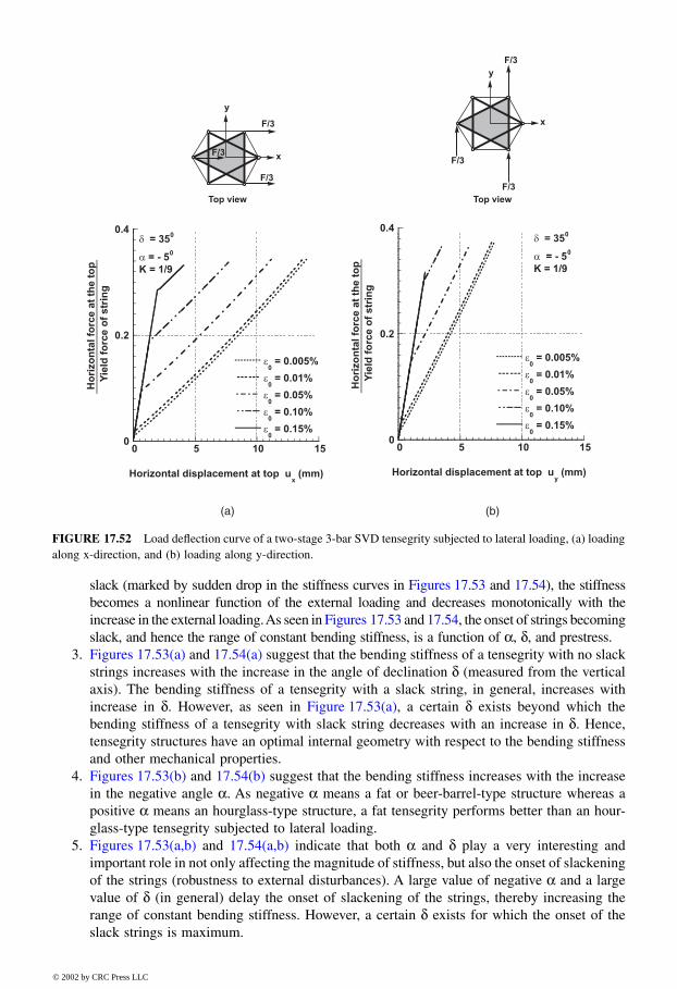
slack (marked by sudden drop in the stiffness curves in Figures 17.53 and 17.54), the stiffnessbecomes a nonlinear function of the external loading and decreases monotonically with theincrease in the external loading. As seen in Figures 17.53 and 17.54, the onset of strings becomingslack, and hence the range of constant bending stiffness, is a function of α, δ, and prestress.

3. Figures 17.53(a) and 17.54(a) suggest that the bending stiffness of a tensegrity with no slackstrings increases with the increase in the angle of declination δ (measured from the verticalaxis). The bending stiffness of a tensegrity with a slack string, in general, increases withincrease in δ. However, as seen in Figure 17.53(a), a certain δ exists beyond which thebending stiffness of a tensegrity with slack string decreases with an increase in δ. Hence,tensegrity structures have an optimal internal geometry with respect to the bending stiffnessand other mechanical properties.

4. Figures 17.53(b) and 17.54(b) suggest that the bending stiffness increases with the increasein the negative angle α. As negative α means a fat or beer-barrel-type structure whereas apositive α means an hourglass-type structure, a fat tensegrity performs better than an hour-glass-type tensegrity subjected to lateral loading.

5. Figures 17.53(a,b) and 17.54(a,b) indicate that both α and δ play a very interesting andimportant role in not only affecting the magnitude of stiffness, but also the onset of slackeningof the strings (robustness to external disturbances). A large value of negative α and a largevalue of δ (in general) delay the onset of slackening of the strings, thereby increasing therange of constant bending stiffness. However, a certain δ exists for which the onset of theslack strings is maximum.

FIGURE 17.52 Load deflection curve of a two-stage 3-bar SVD tensegrity subjected to lateral loading, (a) loadingalong x-direction, and (b) loading along y-direction.

(a) (b)



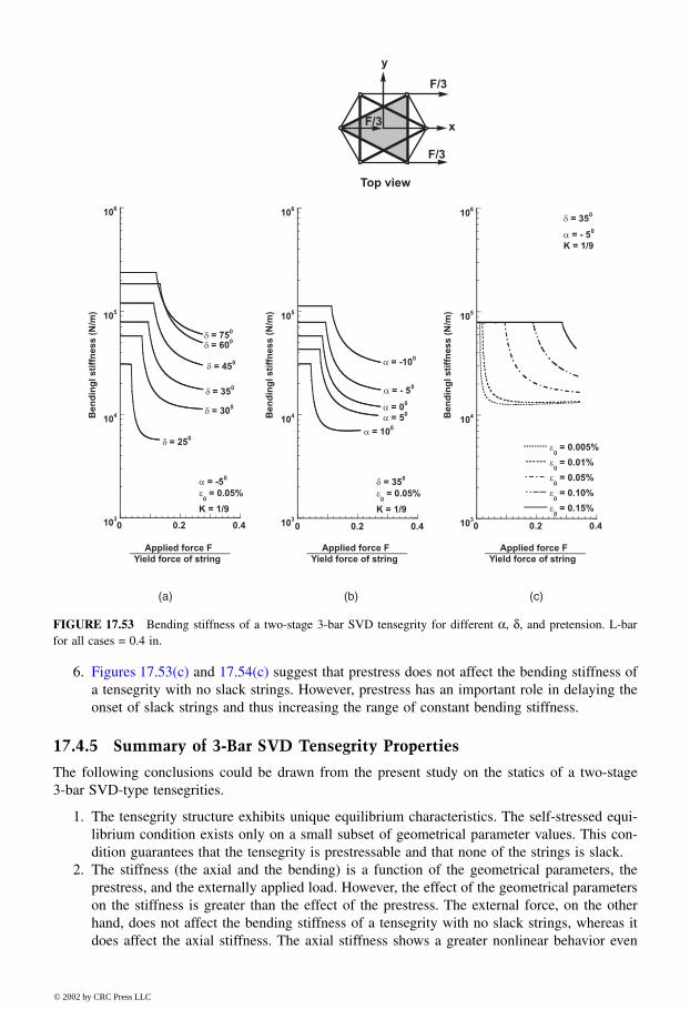
6. Figures 17.53(c) and 17.54(c) suggest that prestress does not affect the bending stiffness ofa tensegrity with no slack strings. However, prestress has an important role in delaying theonset of slack strings and thus increasing the range of constant bending stiffness.

17.4.5 Summary of 3-Bar SVD Tensegrity Properties

The following conclusions could be drawn from the present study on the statics of a two-stage3-bar SVD-type tensegrities.

1. The tensegrity structure exhibits unique equilibrium characteristics. The self-stressed equi-librium condition exists only on a small subset of geometrical parameter values. This con-dition guarantees that the tensegrity is prestressable and that none of the strings is slack.

2. The stiffness (the axial and the bending) is a function of the geometrical parameters, theprestress, and the externally applied load. However, the effect of the geometrical parameterson the stiffness is greater than the effect of the prestress. The external force, on the otherhand, does not affect the bending stiffness of a tensegrity with no slack strings, whereas itdoes affect the axial stiffness. The axial stiffness shows a greater nonlinear behavior even

FIGURE 17.53 Bending stiffness of a two-stage 3-bar SVD tensegrity for different α, δ, and pretension. L-barfor all cases = 0.4 in.

(a) (b) (c)



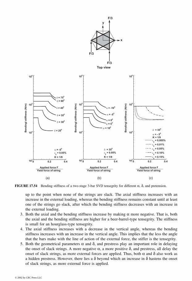
up to the point when none of the strings are slack. The axial stiffness increases with anincrease in the external loading, whereas the bending stiffness remains constant until at leastone of the strings go slack, after which the bending stiffness decreases with an increase inthe external loading.

3. Both the axial and the bending stiffness increase by making α more negative. That is, boththe axial and the bending stiffness are higher for a beer-barrel-type tensegrity. The stiffnessis small for an hourglass-type tensegrity.

4. The axial stiffness increases with a decrease in the vertical angle, whereas the bendingstiffness increases with an increase in the vertical angle. This implies that the less the anglethat the bars make with the line of action of the external force, the stiffer is the tensegrity.

5. Both the geometrical parameters α and δ, and prestress play an important role in delayingthe onset of slack strings. A more negative α, a more positive δ, and prestress, all delay theonset of slack strings, as more external forces are applied. Thus, both α and δ also work asa hidden prestress. However, there lies a δ beyond which an increase in δ hastens the onsetof slack strings, as more external force is applied.

FIGURE 17.54 Bending stiffness of a two-stage 3-bar SVD tensegrity for different α, δ, and pretension.

(a) (b) (c)



17.5 Concluding Remarks

Tensegrity structures present a remarkable blend of geometry and mechanics. Out of variousavailable combinations of geometrical parameters, only a small subset exists that guarantees theexistence of the tensegrity. The choice of these parameters dictates the mechanical properties ofthe structure. The choice of the geometrical parameters has a great influence on the stiffness.Pretension serves the important role of maintaining stiffness until a string goes slack. The geomet-rical parameters not only affect the magnitude of the stiffness either with or without slack strings,but also affect the onset of slack strings. We now list the major findings of this chapter.

17.5.1 Pretension vs. Stiffness Principle

This principle states that increased pretension increases robustness to uncertain disturbances. Moreprecisely, for all situations we have seen (except for the C4T2):

When a load is applied to a tensegrity structure, the stiffness does not decrease as the loadingforce increases unless a string goes slack.

The effect of the pretension on the stiffness of a tensegrity without slack strings is almost negligible.The bending stiffness of a tensegrity without slack strings is not affected appreciably by prestress.

17.5.2 Small Control Energy Principle

The second principle is that the shape of the structure can be changed with very little control energy.This is because shape changes are achieved by changing the equilibrium of the structure. In thiscase, control energy is not required to hold the new shape. This is in contrast to the control ofclassical structures, where shape changes required control energy to work against the old equilibrium.

17.5.3 Mass vs. Strength

This chapter also considered the issue of strength vs. mass of tensegrity structures. We found planarexamples to be very informative. We considered two types of strength: the size of bending forcesand the size of compressive forces required to break the object. We studied the ratio of bendingstrength to mass and compression strength to mass. We compared this for two planar structures,one the C2T4 unit and the other a C4T1 unit, to a solid rectangular bar of the same mass.

We find:

• Reasonably constructed C2T4 units are stronger in bending than a rectangular bar, but theyare weaker under compression.

• The C2T4 has worse strength under compression than a solid rectangular bar.

• The simple analysis we did indicates that C4T2 and C4T1 structures with reasonably chosenproportions have larger compression strength-to-mass ratios than a solid bar.

• On the other hand, a C4T1, while strong (not easily broken), need not be an extremely stiffstructure.

• C4T2 and C4T1 structures can be designed for minimal mass subjected to a constraint onboth strength and stiffness.

It is possible to amplify the effects stated above by the use of self-similar constructions:

• A 2D Tensegrity Beam. After analyzing a C2T4 tensegrity unit, we lay n of them side byside to form a beam. In principle, we find that one can build beams with arbitrarily greatbending strength. In practice, this requires more study. However, the favorable bendingproperties found for C2T4 bode well for tensegrity beams.



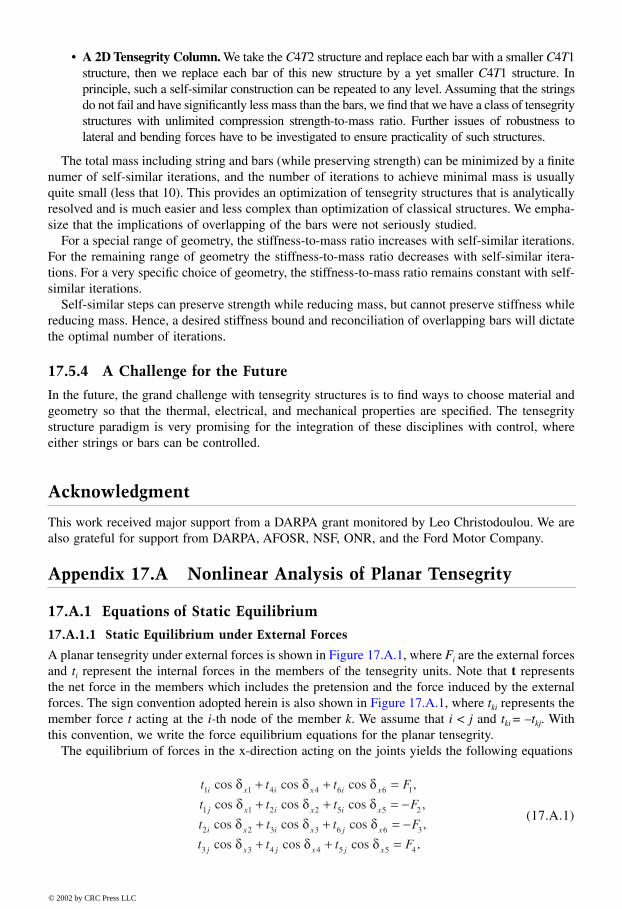
• A 2D Tensegrity Column. We take the C4T2 structure and replace each bar with a smaller C4T1structure, then we replace each bar of this new structure by a yet smaller C4T1 structure. Inprinciple, such a self-similar construction can be repeated to any level. Assuming that the stringsdo not fail and have significantly less mass than the bars, we find that we have a class of tensegritystructures with unlimited compression strength-to-mass ratio. Further issues of robustness tolateral and bending forces have to be investigated to ensure practicality of such structures.

The total mass including string and bars (while preserving strength) can be minimized by a finitenumer of self-similar iterations, and the number of iterations to achieve minimal mass is usuallyquite small (less that 10). This provides an optimization of tensegrity structures that is analyticallyresolved and is much easier and less complex than optimization of classical structures. We empha-size that the implications of overlapping of the bars were not seriously studied.

For a special range of geometry, the stiffness-to-mass ratio increases with self-similar iterations.For the remaining range of geometry the stiffness-to-mass ratio decreases with self-similar itera-tions. For a very specific choice of geometry, the stiffness-to-mass ratio remains constant with self-similar iterations.

Self-similar steps can preserve strength while reducing mass, but cannot preserve stiffness whilereducing mass. Hence, a desired stiffness bound and reconciliation of overlapping bars will dictatethe optimal number of iterations.

17.5.4 A Challenge for the Future

In the future, the grand challenge with tensegrity structures is to find ways to choose material andgeometry so that the thermal, electrical, and mechanical properties are specified. The tensegritystructure paradigm is very promising for the integration of these disciplines with control, whereeither strings or bars can be controlled.

Acknowledgment

This work received major support from a DARPA grant monitored by Leo Christodoulou. We arealso grateful for support from DARPA, AFOSR, NSF, ONR, and the Ford Motor Company.

Appendix 17.A Nonlinear Analysis of Planar Tensegrity

17.A.1 Equations of Static Equilibrium

17.A.1.1 Static Equilibrium under External Forces

A planar tensegrity under external forces is shown in Figure 17.A.1, where Fi are the external forcesand ti represent the internal forces in the members of the tensegrity units. Note that t representsthe net force in the members which includes the pretension and the force induced by the externalforces. The sign convention adopted herein is also shown in Figure 17.A.1, where tki represents themember force t acting at the i-th node of the member k. We assume that i < j and tki = –tkj. Withthis convention, we write the force equilibrium equations for the planar tensegrity.

The equilibrium of forces in the x-direction acting on the joints yields the following equations

(17.A.1)

t t t F

t t t F

t t t F

t t t F

i x i x i x

j x i x i x

i x i x j x

j x j x j x

1 1 4 4 6 6 1

1 1 2 2 5 5 2

2 2 3 3 6 6 3

3 3 4 4 5 5 4

cos cos cos

cos cos cos

cos cos cos

cos cos cos

δ δ δδ δ δδ δ δδ δ δ

+ + =+ + = −+ + = −+ + =

,

,

,

..



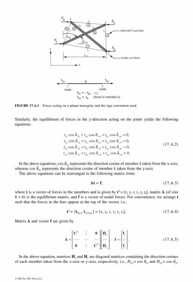
Similarly, the equilibrium of forces in the y-direction acting on the joints yields the followingequations

(17.A.2)

In the above equations, cos δxk represents the direction cosine of member k taken from the x-axis,whereas cos δyk represents the direction cosine of member k taken from the y-axis.

The above equations can be rearranged in the following matrix form:

At = f, (17.A.3)

where t is a vector of forces in the members and is given by tT = [t1 t2 t3 t4 t5 t6], matrix A (of size8 × 6) is the equilibrium matrix, and f is a vector of nodal forces. For convenience, we arrange tsuch that the forces in the bars appear at the top of the vector, i.e.,

tT = [tbars tstrings] = [t5 t6 t1 t2 t3 t4]. (17.A.4)

Matrix A and vector f are given by

(17.A.5)

In the above equation, matrices Hx and Hy are diagonal matrices containing the direction cosinesof each member taken from the x-axis or y-axis, respectively, i.e., Hxii = cos δxi and Hyii = cos δyi.

FIGURE 17.A.1 Forces acting on a planar tensegrity and the sign convention used.

t t t

t t t

t t t

t t t

i y i y i y

j y i y i y

i y i y j y

j y j y j y

1 1 4 4 6 6

1 1 2 2 5 5

2 2 3 3 6 6

3 3 4 4 5 5

0

0

0

0

cos cos cos

cos cos cos

cos cos cos

cos cos cos

δ δ δδ δ δδ δ δδ δ δ

+ + =+ + =+ + =+ + =

,

,

,

.

A

C 0

0 C

H

H

f

f

f

=

=

T

T

x

y

x

y

M

L L L

M

L L, .



Similar to the arrangement of t, Hx and Hy are also arranged such that the direction cosines of barsappear at the top of Hx and Hy whereas the direction cosines of strings appear at the bottom of Hx

and Hy. Vectors fx and fy are the nodal forces acting on the nodes along x- and y-axes, respectively.Matrix C is a 6 × 4 (number of members × number of nodes) matrix. The k-th row of matrix Ccontains –1 (for i-th node of the k-th member), +1 (for j-th node of the k-th member) and 0. MatrixC for the present case is given as

(17.A.6)

It should be noted here that matrix A is a nonlinear function of the geometry of the tensegrity unit, thenonlinearity being induced by the matrices Hx and Hy containing the direction cosines of the members.

17.A.2 Solution of the Nonlinear Equation of Static Equilibrium

Because the equilibrium equation given in (17.A.3) is nonlinear and also A (of size 8 × 6) is nota square matrix, we solve the problem in the following way.

Let be the member forces induced by the external force f, then from (17.A.3)

(17.A.7)

where e is the deformation from the initial prestressed condition of each member, and from Hooke’slaw = Ke, where K is a diagonal matrix of size 6 × 6, with Kii = (EA)i/Li. (EA)i and Li are theaxial rigidity and the length of the i-th member. Note that A expressed above is composed of boththe original A0 and the change in A0 caused by the external forces f.

A = A0 + Ã (17.A.8)

where Ã is the change in A0 caused by the external forces f.The nonlinear equation given above can be linearized in the neighborhood of an equilibrium. In

the neighborhood of the equilibrium, we have the linearized relationship,

(17.A.9)

Let the external force f be gradually increased in small increments (fk = fk-1 + ∆f at the k-th step),and the equilibrium of the planar tensegrity be satisfied for each incremental force, then (17.A.7)can be written as

A(uk)KA (uk)T uk = fk – A(uk)t0 (17.A.10)

The standard Newton–Raphson method can now be used to evaluate uk of (17.A.10) for eachincremental load step ∆∆∆∆fk. The external force is gradually applied until it reaches its specific value

C =

−−−

−−

−

0 1 0 1

1 0 1 0

1 1 0 0

0 1 1 0

0 0 1 1

1 0 0 1

Bars

Strings

t

At f

A t t f

At f At

AKe f At

=⇒ + =⇒ = −⇒ = −

( )0

0

0

˜

˜

t

e A uk kT

k=



and uk is evaluated at every load step. Matrix A, which is now a nonlinear function of u, is updatedduring each load step.

To compute the external force that would be required to buckle the bars in the tensegrity unit,we must estimate the force being transferred to the bars. The estimation of the compressive forcein the bars following full nonlinear analysis can be done numerically. However, in the followingwe seek to find an analytical expression for the compressive force in the bars. For this we adopt alinear and small displacement theory. Thus, the results that follow are valid only for small displace-ment and small deformation.



Appendix 17.B Linear Analysis of Planar Tensegrity

17.B.1 EI of the Tensegrity Unit with Slack Top String

17.B.1.1 Forces in the Members

A tensegrity with a slack top string does not have prestress. As mentioned earlier, we adopt thesmall displacement assumptions, which imply that the change in the angle δ due to the externalforces is negligible. Therefore, in the following, we assume that δ remains constant. The memberforces in this case are obtained as

(17.B.1)

The strain energy in each of the members is computed as

(17.B.2)

The total strain energy is then obtained as

(17.B.3)

where K is defined as

(17.B.4)

t F

t F

t

t F

tF

tF

1

2

3

4

5

6

2

0

=

=

=

=

= −

= −

,

,

,

,

.

tan ,

tan

cos

cos

δ

δ

δ

δ

UL F

EA

UL F

EA

U

UL F

EA

UL F

EA

UL F

EA

s

s

s

b

b

10

2

20

2

3

40

2

50

2

60

2

12

4

12

0

12

12

12

=

=

=

=

=

=

( ),

( ),

,

( ),

( ),

( ).

tan

tan

cos

cos

3

3

3

3

δ

δ

δ

δ

U UL

EA

FKi

si

= = + +∑ 12

220

2

( )[ ],

cossin cos3

3 3

δδ δ

KEA

EAs

b

=( )

( ).



Thus, large values of K mean that the strings are stiffer than the bars, whereas small values of Kmean that the bars are stiffer than the strings. K → 0 means bars are rigid.

17.B.1.2 External Work and Displacement

External work W is given by

(17.B.5)

where u is the displacement as shown in Figure 17.11.Equating the total strain energy given by (17.B.3) to the work done by the external forces given

by (17.B.5), and then solving for u yields

(17.B.6)

17.B.1.3 Effective EI

Because EI = Mρ, we have

(17.B.7)

Substitution of from (17.B.6) into (17.B.7) yields

(17.B.8)

Substituting L0 = Lbar cos δ in (17.B.7) and (17.B.8) yields the following expressions for theequivalent bending rigidity of the planar section in terms of the length of the bars Lbar,

(17.B.9)

or equivalently,

(17.B.10)

W Fu Fu= =412

2 ,

uFL

EAK

s

= + +0

22

( )[ ].

cossin cos3

3 3

δδ δ

EI FLL

u=

0

02

2tan tan

1δ δ .

u

EIL EA

Ks=

+ +12 2

02

3

( ) cos

( cos ).

sin

sin

2

3

δ δδ δ

EI FLL

ubarbar=

sin cos sin1δ δ δ

2

2

.

EIL EA

Kbar s=

+ +12 2

2

3

( )

(sin ).

sin cos

cos

2 3

3

δ δ

δ δ



Appendix 17.C Derivation of Stiffness of the C4T1i Structure

17.C.1 Derivation of Stiffness Equation

For a C4T1i structure under the buckling load F, the compressive load of bar in the i-th iteration is

(17.C.1)

Similarly, the tension of strings in the i-th iteration is

(17.C.2)

So, the buckling load F can be written in terms of any one of the compressive bar loads or tensionof strings in i-th iteration

(17.C.3)

From the geometry of the structure,

(17.C.4)

Equation (17.C.3) can be simplified to

(17.C.5)

From this,

(17.C.6)

This means the force-to-length ratio of every compressive or tensile members is the same. It isassumed that all the bars and strings have constant stiffness and, hence, are linear. With thisassumption,

(17.C.7)

So (17.C.6) becomes

(17.C.8)

FF

i

ji

j

==∏ cos12 δ

.

tF

j i ijj

sj

s

= = −=∏

2

21 2 3 1

1

sinfor

δ

δcos, , , ..., , .

F Ft

j i ii sj

jp

p

j

s

i

= = = −==

∏∏22

2 1 2 3 111

cos sin

for δδ

δcos , , , ..., , .

sinδ

δ

jtj

j

jj

j

L

L

L

L

=

= −

2

21

,

cos .

F FL

Lt

L

Lii

jtj

= =0 0 .

F

L

F

L

t

L

t

Li

i

j

tj t0

1

1

= = = .

F k L L

t k L L

i bi i i

j tj tj tj

= −

= −

( ),

( ).

0

0

kL

Lk

L

Lk

L

Lbii

itj

tj

tjt

t

t

0 01

10

1

1 1 1−

= −

= −

.



Taking the infinitesimal of all the length quantities yields

and hence,

(17.C.9)

From the geometry of the structure,

(17.C.10)

Taking the infinitesimal of (17.C.10), noting that Li is length of bars, yields

(17.C.11)

Combining the (17.C.11) with (17.C.9) yields

(17.C.12)

From (17.C.5), it is natural to choose F in terms of the tension in the first iteration, i.e.,

The derivative of F w.r.t. L0 yields

(17.C.13)

With (17.C.12), the stiffness of C4T1i will be

(17.C.14)

− = =kL

LdL k

L

LdL k

L

LdLbi

i

ii tj

tj

tjtj t

t

tt

02

02 1

10

12 1,

dLk L

k L

L

LdL

dLk L

k L

L

LdL

it t

bi i

i

tt

tjt t

tj tj

tj

tt

= −

=

1 10

0

2

12 1

1 10

0

2

12 1

,

.

L L L

L L L

L L

t

t t

ii

jtj

j

i

02

12

12

22

22

12

2 1 2

1

4

4 4

4 4

= −

= − −

=

= − −

=∑

( )

...

.

dLL

LdL

LL dLi i

ij

tj tj

j

i

00 0

1

1

41

4= − −

=∑ .

dL

dL

k L

L L

L

k L

L

k Lt

t t

t

i i

bi i

j tj

tj tjj

i

0

1

1 10

0 12

3

0

13

01

4 4= +

−

=∑ .

F tL

Lk

L

LL

tt

t

t

= = −

10

11

10

101 .

dF

dLk

L

Lk L

L

L

dL

dLtt

tt

t

t

t

01

10

11 0

10

12

1

0

1= −

+ .

KdF

dLk

L

LL

L

k L

L

k L

kL

L

k

k

L

L

L

L

k

i tt

t

i i

bi i

j

j

itj

tj tj

tt

t

i t

bi

i

i

i j t

= − = −

+ +

= −

+

+

−

=

−

−

∑0

110

102

3

0

1

1

3

0

1

110

1

1

0 0

2

1 1

1 4 4

1 4 4kk

L

L

L

Ltj

tj

tj

tj

j

i

0 0

2

1

1

=

−

∑ .



17.C.2 Some Mathematical Relations in Buckling Design

In the strength-preserving design, the C4T1i system is designed to buckle at the same load as theoriginal bar C4T10. The angles δj, where j = 1, 2, …, i–1, i are free variables to be specified to fixthe geometry. Therefore, it is important to find out all the lengths and ratio quantities in terms ofthese angles.

17.C.2.1 Length of Structure and Strings

From the geometry of the structure, it can be shown that

(17.C.15)

17.C.2.2 Computing the Stiffness Ratio of Strings,

Consider the ratio

From (17.109)

With (17.C.2) and (17.C.15), the ratio can be simplified to

From this,

(17.C.16)

In particular, if Etj = Et and σtj = σt, then

(17.C.17)

L L

L L

i si

s

tj i j s ji

s

0 1

1

2

2 2

=

=

=

= +

∏∏cos ,

sin cos .

δ

δ δ

k

kfor s j i its

tj

, , , ,..., ,= −1 2 3 1

k

k

E A

L

L

E A

E

E

r

r

L

L

t j

tj

t j t j

t j

tj

tj tj

t j

tj

t j

tj

tj

t j

( ) ( ) ( )

( )

( ) ( )

( )

.

+ + +

+

+ +

+

=

=

1 1 1

1

1 12

21

ππ

k

k

E

E

t

t

L

Lt j

tj

t j

tj

tj j

t j j

tj

t j

( ) ( )

( ) ( )

.+ + +

+ +

=

1 1 1

1 1

σσ

k

k

E

Et j

tj

t j

tj

tj

t j

( ) ( )

( )

.+ +

+

=

1 1

1

σσ

k

k

E

Ets

tj

ts tj

tj ts

=σσ

.

k

kts

tj

= 1.



So, in the strength-preserving design, if the same material is used, then all strings have the samestiffness.

17.C.2.3 Computing the Stiffness Ratio of String to Bar

The stiffness of bar and strings are defined by

where E is the Young’s modulus, A is the cross-section area, and L is the length of bar or stringsat the buckling load. With this definition and (17.C.16),

From (17.106), (17.109), and (17.C.15),

Substitute F from (17.66) into the above equation to obtain

(17.C.18)

For some materials of bars and strings, (17.C.18) reduces to

(17.C.19)

17.C.2.4 Computing the Rest Length-to-Length Ratio of Strings, Ltj0/Ltj

The tension in the strings is given by

k

kj i itj

bi

where = −1 2 3 1, , ,..., ,

kEA

L= ,

k

k

k

k

k

k

E

E

E r

L

L

E r

E

E L L

L

rr

tj

bi

tj

ti

ti

bi

tj ti

ti tj

ti ti

ti

i

i

tj ti

i tj ti i

i

iti

i

= =

=

σσ

ππ

σσ

2

2

2

221.

k

k

E

E

t l

L

E

E

F

L

E

El

tj

bi

tj ti

i tj

i

ti

i

i i

tj ti

i tj

i

ti si

s i i

i

pi

p

=

=

= =

σσ πσ δ

σσ

δπσ δ δ δ

4

2

2

22 1

2

2

2

12

0

1

2

1

1

2

0

sin

sin

cos sin cosΠ Π22 .

k

k

E

l

E

Etj

bi

tj

tj is

s

i

=

=∏π

σδ

2

02

0

1

12

162cos .

k

k

E

ltj

bi

tj

tjs

s

i

=

=∏π

σδ

2

02

1

12

162cos .



From (17.109),

So,

(17.C.20)

17.C.2.5 Computing the Rest Length to Length Ratio of Bars, Li0 /Li

From (17.C.6),

Hence,

leading to

(17.C.21)

Using (17.C.20) and (17.C.21) reduces to

(17.C.22)

17.C.2.6 Computing the String Stiffness, kt1

Recall that the string stiffness is given by

Using (17.66), (17.108), and (17.109) yields

t k L L

tE r

LL L

j tj tj tj

jtj tj

tjtj tj

= −

= −

( ),

( ).

0

2

0

π

tE t

LL Lj

tj j

tj tjtj tj= −

σ( ).0

L

L Etj

tj

tj

tj

0 1= −σ

.

F

L

t

Li

i t

= 1

1

kL

Lk

L

Lbii

it

t

t

01

10

1

1 1−

= −

L

L

k

k

L

Lio

i

t

bi

t

t

= + −

1 11 10

1

.

L

L

k

k Ei

i

t

bi

t

t

0 1 1

1

1= +σ

.

kE r

L

t

tt t

t1

1 12

1

2

021

1161

=

= +

π.



(17.C.23)

References

1. K. Snelson, Continuous tension, discontinous compression structures, US Patent 3, 169, 611, 1965.2. B. Fuller. Tensile-integrity structures, US Patent, 3, 063, 521, 1962.3. R. Adhikari, R. E. Skelton, and W. J. Helton, Mechanics of Tensegrity Beams, UCSD, Structural

System and Control Lab., Report No. 1998-1, 1998.4. D. M. Campbell, D. Chen, P. A. Gossen, and K. P. Hamilton, Effects of spatial triangulation on

the behavior of “tensegrity” domes, 652–663, IASS-ASCE International Symposium, April 24–28,Atlanta, GA, 1994.

5. R. Chu, Tensegrity, Journal of Synergetics, 2(l), 1988.6. M. F. Coughlin and D. Stamenovic, A tensegrity structure with buckling compression elements:

Application to cell mechanics, Transactions of ASME, Journal of Applied Mechanics, 64, 480–486,1997.

7. D. E. Ingber, Tensegrity: The architectural basis of cellular mechanotransduction, Annual Reviewof Physiology, 59, 575–599, 1997.

8. I. J. Oppenheim and W. J. Williams, Tensegrity prisms as adaptive structures, ASME Annualmeeting, Dallas, November 1997.

9. A. Pugh, An Introduction to Tensegrity, University of California Press, Berkeley, 1976.10. R. Motro et al., Form finding numerical methods for tensegrity systems, IASS-ASCE International

Symposium, Atlanta, GA, April 24–28, 706–713, 1994.11. H. Faruya, Concept of deployable tensegrity structures in space applications, International Journal

of Space Structures, 7(2), 143–151, 1992.12. S. Pellegrino, Analysis of prestressed mechanisms, International Journal of Solids and Structures,

26(12), 1329–1350, 1989.13. S. Pellegrino, A class of tensegrity domes, International Journal of Space Structures, 7(2), 1992.14. A. Hanaor, Double-layer tensegrity grids as deployable structures, International Journal of Space

Structures, 8, 1992.15. S. Pellegrino, Foldable bar structures, International Journal of Solids and Structures, 34(15),

1825–1847, 1996.16. D. Williamson and R. E. Skelton, A general class of tensegrity systems: Equilibrium analysis,

Engineering Mechanics for the 21st Century, ASCE Conference, La Jolla, 1998.17. R. E. Skelton, J. P. Pinaud, and D. L. Mingori, Dynamics of the shell class of tensegrity structures,

Journal of the Franklin Institute, 338(2–3), 255–320, 2001.18. H. Murakami and Y. Nishimura, Static and dynamic characterization of regular truncated icosa-

hedral and dodecahedral tensegrity modules, International Journal of Solids and Structures, 2001(to appear).

19. B. de Jager and R. E. Skelton, Optimizing stiffness properties of tensegrity structures, Proceedingsof International Mechanical Engineering Congress and Exposition, 3330, New York, 2001.

20. C. Sultan, Modeling, design, and control of tensegrity structures with applications, Ph.D. disser-tation, Purdue University, Lafayette, Indiana, 1999.

kE

L

t

E F

L

E E r

L

E E L

l

tt

t t

t

t

t

t

t

t

11

1

1

1

1

1

1

0 1

1

1

03

04

03

0 13

0

1 04

4

64

=

=

=

=

σ

σδδ

σπ

πσ

tan

.

tan



21. C. Sultan, M. Corless, and R. E. Skelton, The prestressability problem of tensegrity structures:Some analytical solutions, International Journal of Solids and Structures, 2001 (to appear).

22. C. Sultan, M. Corless, and R. E. Skelton, Tensegrity flight simulator, Journal of Guidance, Control,and Dynamics, 23(6), 1055–1064, 2000.

23. C. Sultan, M. Corless, and R. E. Skelton. Linear dynamics of tensegrity structures, EngineeringStructures, 2001 (to appear).

24. C. Sultan, M. Corless, and R. E. Skelton, Symmetrical reconfiguration of tensegrity structures,International Journal of Solids and Structures, 2001 (to appear).

25. L. Caviglione, Modellazione statica e dinamica di una tensegrity nell’ambito di una strategia dicontrollo attivo, Laurea thesis, University of Genoa, 1999.

26. M. Pedretti, Smart tensegrity structures for the Swiss expo, Smart Structures and Materials, 3330,San Diego, 1998.

27. L. Caviglione, A. Del Grosso, and M. Pedretti, Stabilisation and control of large tensegritystructures, private communication.

28. A. G. M. Michell, The limits of economy in frame structures, Philosophical Magazine, 8, 589–597,1904.

29. M. P. Bendsoc and N. Kikuchi, Generating optimal topologies in structural design using ahomozenization method, Computer Methods in Applied Mechanics and Engineering, 71, 197–224,1988.

30. F. Jarre, M. Koevara, and J. Zowe, Optimal truss design by interior-point methods, SIAM Journalon Optimization, 8(4), 1084–1107, 1998.

31. J. Lu and R. E. Skelton, Optimal hybrid control for structures, Computer-Aided Civil and Infra-structure Engineering, 13, 405–414, 1998.

32. A. H. Simmons, C. A. Michal, and L. W. Jelinski, Molecular orientation and two-component natureof the crystalline fraction of dragline silk, Science, 271, 84–87, 1996.

33. Y. Termonia, Molecular modeling of spider silk elasticity, Macromolecules, 27, 7378–7381, 1994.34. D. E. Ingber, Architecture of life, Scientific American, 48–57, January 1998.35. D. E. Ingber, Cellular tensegrity: Defining new rules of biological design that govern the cyto-

skeleton, Journal of Cell Science, 104(3), 613–627, 1993.36. R.E. Skelton, Dynamic Systems Control — Linear Systems Analysis and Synthesis, John Wiley &

Sons, New York, 1988.37. S. Pellegrino and C. R. Calladine, Matrix analysis of statistically and kinematically indeterminate

frameworks, International Journal of Solids and Structures, 22(4), 409–428, 1985.



dynamics and control of aerospace systems - ucsd …helton/billspapersscanned/shapc01.pdfsvd...

Documents