revised version forthcoming in the Journal of International Economics

Trade Deflection and Trade Depression†

Chad P. Bown Meredith A. Crowley

Brandeis University Federal Reserve Bank of Chicago

This version: September 2006

Original version: November 2003

Abstract

This is the first paper to empirically examine whether a country’s use of an import restrictingtrade policy distorts a foreign country’s exports to third markets. We first develop a theoretical modelof worldwide trade in which the imposition of antidumping and safeguard tariffs, or “trade remedies,” byone country causes significant distortions in world trade flows. We then empirically test this model byinvestigating the effect of the United States’ use of such import restrictions on Japanese exports of roughly4800 products into 37 countries between 1992 and 2001. Our estimation yields evidence that US restrictionsboth deflect and depress Japanese export flows to third countries. Imposition of a US antidumping measureagainst Japan deflects trade, as the average antidumping duty on Japanese exports leads to a 5-7% increasein Japanese exports of the same product to the average third country market. The imposition of a USantidumping measure against a third country depresses trade, as the average US duty imposed on a thirdcountry leads to a 5-19% decrease in Japanese exports of that same product to the average third country’smarket. We also document the substantial variation in trade deflection and trade depression across differentimporting countries and exported products.

JEL No. F10, F12, F13Keywords: Deflected Trade, Depressed Trade, Antidumping, Safeguards, MFN

†Bown (corresponding author): Department of Economics and International Business School, MS 021,Brandeis University, Waltham, MA 02454-9110 USA tel: 781-736-4823, fax: 781-736-2269,email: cbown@brandeis.edu, web: http://www.brandeis.edu/̃cbown/

Crowley: Department of Economic Research, Federal Reserve Bank of Chicago, 230 S. LaSalle St, Chicago,IL 60604-1413 USA tel: 312-322-5856, fax: 312-322-2357, email: mcrowley@frbchi.org

1 Introduction

In March 2002, the United States imposed a “safeguard” - a broad-based set of tariffs and quotas - on imports

of steel to shield its domestic industry from foreign competition. Shortly thereafter, the European Union and a

number of other steel-importing countries responded by imposing their own import restrictions on steel.1 The

EU partially justified its trade policy by arguing that the change in US trade policy would re-route or “deflect”

Asian steel exports - initially destined for the newly closed US market - to what would have otherwise been a

relatively open EU market.2

Are the EU’s concerns in the steel case consistent with historical experience? When a large importing

country, such as the US, uses import restrictions such as a safeguard or antidumping duties to protect domestic

producers from imports, does this lead to the substantial deflection of exports to third country markets like the

EU? To our knowledge, this is the first paper to address this question empirically. We begin by presenting a

simple theoretical model to illustrate the EU’s argument on deflected trade. This model embodies the potential

differential impact on world trade flows of a country-specific antidumping duty (AD) versus a nondiscriminatory

safeguard measure (SG).3 We then test the model’s implications on a panel of Japanese product-level exports

from 1992-2001 that is matched at the product level to changes in US trade policy through the application of

antidumping duties and safeguard measures. We investigate whether there is evidence that the US use of such

AD and SG “trade remedies” has an impact on Japanese export patterns to third markets and then whether1In addition to the EU, other WTO members that imposed at least preliminary safeguard protection on steel products between

March 2002 and October 2003 included Chile, China, Czech Republic, Hungary, Poland and Venezuela (WTO, 2002 and 2003).

Canada and Bulgaria had also initiated steel safeguard investigations after the US imposition of protection but did not apply

protection.2The 25 March 2002 EU press release announcing its steel safeguard response to the US steel safeguard of 5 March noted that

“[w]hilst US imports of steel have fallen by 33% since 1998, EU imports have risen by 18%. Given that worldwide there are 2

major steel markets (EU with 26.6m tonnes of imports in 2001 and US with 27.6m tonnes), this additional protection of the US

steel market will inevitably result in gravitation of steel from the rest of the world to the EU. This diversion is estimated to be as

much as 15m tonnes per year (56% of current import levels).” (European Union, 2002)3A ‘nondiscriminatory’ trade policy (tariff) is one that is applied equally to all importing countries, e.g., all imports into a

country face the same tariff rate. The term most-favored-nation (MFN) will be synonymous with ‘nondiscriminatory’ for the

purpose of this paper. A ‘discriminatory’ or ‘preferential’ trade policy is one in which an importing country applies different

tariffs to imports from different exporting countries. For example, the import tariff on goods from regional trade agreement

partners is usually lower than that imposed on goods from other countries. Although the WTO requires that all its members have

nondiscriminatory trade policies, there are numerous exceptions to this rule. Two of the most important exceptions in practice

are that the WTO allows for discriminatory tariffs when countries participate in preferential trade agreements and when countries

impose antidumping duties.

1

there is variation across importing countries and/or products of the size of any potential distortions.

In the empirical investigation, we use a dynamic panel data model to estimate the impact of US import

restrictions on Japanese exports to third countries. We construct a dataset of Japanese exports of roughly

4800 products into 37 countries between 1992 and 2001 to assess the effect of US import restrictions, thus

exploiting the substantial variation across products and time of Japanese exports to third countries. Our

empirical approach allows us to estimate the impact of a US-imposed, Japan-specific antidumping duty on

Japanese exports, identifying whether trade is deflected to third markets. In addition we are able to identify

a second impact of US antidumping duties on Japanese exports; when a US duty is applied against a third

country’s exports, Japanese exports of the targeted product to the third country market are depressed.

Japan is a particularly useful starting point for such an investigation for a variety of reasons. First, Japanese

firms are frequently targeted by US acts of country-specific import protection; e.g., Japanese firms made up

10% of the US antidumping caseload that resulted in duties between 1992 and 2001.4 Over the period of our

sample, the US imposed antidumping duties on 157 unique 6-digit HS products from Japan. Furthermore, US

import restrictions targeting third country exports affected an additional 167 products that Japan exports to

one or more third countries. Second, Japanese exporters are particularly prominent in world trade. Japanese

total exports as a share of world total exports was 7.5% in 1997, the midpoint of our sample.5 Third, as table 1

illustrates, Japanese exports to the US represent a substantial share of Japan’s total exports, i.e., roughly one

quarter of its total exports. This allows for the possibility of substantial trade being deflected to third country

markets after the imposition of a US trade restriction.

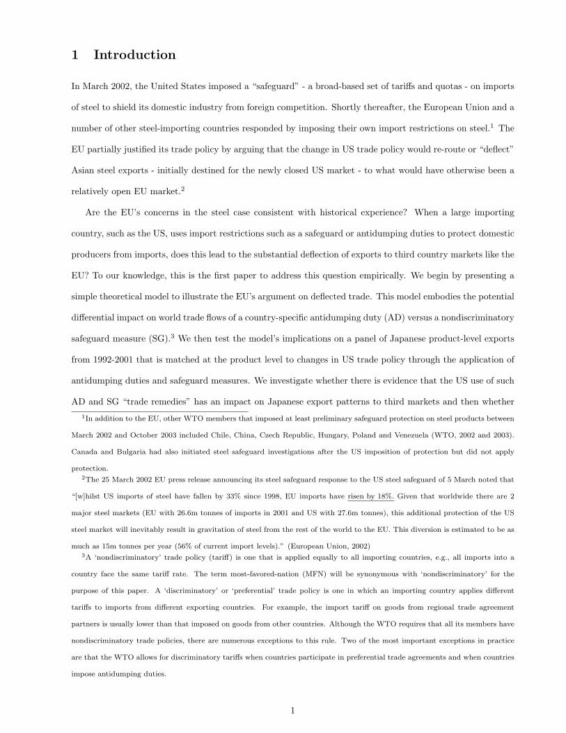
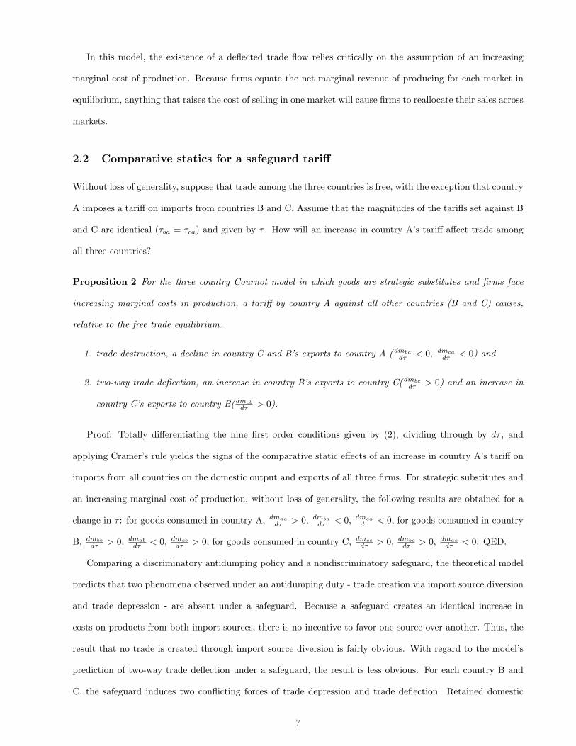
Figure 1 provides a preview of our empirical results on trade deflection and trade depression. The figure

presents the time path of Japanese exports to third country (i.e., non-US) markets of three different categories

of Japanese products: 1) those for which only Japanese firms were hit with a US antidumping measure, 2) those

for which only non-Japanese firms were hit with a US antidumping measure, and 3) those for which no US

antidumping measures were applied. We use the mean growth rates of these three subsamples of observations

to plot the basic pattern in the data over a three year window: the year of the US antidumping investigation,

as well as the two preceding years. For the Japanese products that are the target of US AD cases, there is a

dramatic increase in Japanese exports to third country markets (i.e., “trade deflection”) in the year of the AD

4Japan was actually the second most targeted exporter, when measured as the number of petitions resulting in duties, as China

made up 16% of the caseload.5Japanese exports as a share of world total exports peaked in 1986 at 10.3%. These calculations are based on the data provided

in Feenstra (2000) and include intra-EU trade in the calculation of world total exports.

2

investigation. Furthermore, for the Japanese exports of products to third countries where the third country

exporters were the target of a US AD investigation, there is a substantial reduction (i.e., “trade depression”)

of Japanese exports to that third country in the year of the AD investigation. In this paper we assess whether

the suggestive evidence presented in figure 1 is statistically and economically signicant when we control for

other factors affecting Japan’s product-level export growth.

Our formal econometric results indicate that the imposition of US import restraints over the 1992-2001

period both deflect and depress Japanese export flows to third country markets. Imposition of a US antidumping

duty against Japanese exporters is associated with substantial deflection of trade. For example, the median

antidumping duty against Japan leads to a 5-7% average increase in Japanese exports to a non-US trading

partner. Furthermore, there is also evidence of trade depression. When the median US antidumping duty

is imposed against a third country’s exporters, Japanese exports to the third country in the same product

category decrease by an average of 5-19%. Finally, when faced with a US safeguard measure, Japanese exports

to third countries fall by somewhere between 55% and 70%. Finally, in terms of the policy relevance, these

results provide evidence that the concerns voiced by the EU in their response to the March 2002 act of US

import protection may not be unfounded, given the historical experience with US trade remedies and the

associated Japanese export response.

Our empirical analysis, which examines how a discriminatory trade policy change affects trade flows, fits

broadly into the literature on preferential trade agreements initiated by Viner (1950). Viner identified that

discriminatory trade policies associated with preferential trade agreements (PTAs) had both positive ‘trade

creation’ welfare effects due to the enhanced trade between members (allowing members to exploit compara-

tive advantage amongst themselves) and negative ‘trade diversion’ welfare effects by potentially reducing trade

between members and non-members (and thus preventing the full exploitation of worldwide comparative ad-

vantage). Ultimately, Viner recognized that the overall welfare effect of a PTA would have to be assessed

empirically. More recently, a substantial theoretical literature (including, but not limited to Bond and Sy-

ropoulos, 1996; Bagwell and Staiger, 1997, 1999, 2004; Levy, 1997; Ethier, 2004; and McLaren, 2002) examines

the role of preferential policy exceptions in multilateral trade agreements.6 These papers typically focus on

the import source diversion as the mechanism through which discriminatory trade policies affect welfare; the

domestic welfare losses are derived from importing from someone who is not the lowest cost producer and6For a survey of other recent papers focusing on different theoretical elements of the interaction between preferential and

multilateral agreements, see Krishna (2004). For a literature survey on the nondiscrimination principle and the economic aspects

of the MFN clause in trade agreements, see Horn and Mavroidis (2001).

3

failing to (globally) exploit comparative advantage. In contrast, our analysis will focus on export diversion

where global welfare costs would arise because the low cost exporter is being shut out of a market for which it

would potentially be the most efficient producer if there were non-discriminatory application of tariffs.

Our empirical approach is most similar to Romalis (2002) which investigates the import source diversion of

Mexican and Canadian exports to the US resulting from the North American Free Trade Agreement (NAFTA)

and the earlier Canada-US Free Trade Agreement (CUSFTA), respectively.7 Romalis uses a similarly disag-

gregated panel of product-level export data and finds that Mexican and Canadian shares of US imports have

increased most rapidly in the products facing the largest changes in trade policy; i.e., where the greatest PTA

tariff preferences were conferred. While not the focus of his analysis, in presenting information on two of his

controls, Mexican and Canadian shares of EU imports, he documents evidence that is consistent with our re-

sults regarding the deflection of trade.8 Although related, our paper differs from Romalis’ both in terms of the

question we ask and the empirical methodology we employ. Romalis uses a difference-in-differences approach

to examine if changes in US trade policy (NAFTA and CUSFTA) produced import source diversion. We use

dynamic panel data methods to examine if changes in US trade policy (AD and SG) are associated with the

deflection and also the depression of exports.

With respect to the economics literature on trade remedies, our results on the trade distorting effects of

antidumping measures complement the work of Prusa (1997, 2001).9 Prusa (2001), for example, uses a panel

of US industry-level imports and data on US antidumping measures for 1980-1994 to investigate the import

source diversion that occurs for the United States when a discriminatory trade policy causes importers to

switch from a lower cost to a higher cost foreign supplier. He provides evidence that foreign exporters in an

industry subject to a US AD measure who are not-named in an antidumping petition increase exports to the

US in conjunction with the exports of the country targeted by the AD petition falling. Our paper can provide

insight as to where the products targeted by the US petition go, since they are no longer being exported to

the US market.10

7Clausing (2001) is another recent paper that looks at the trade creation and trade diversion effects of the CUSFTA through an

analysis of a panel on product-level trade data and tariff changes. Romalis (2002) presents a thorough discussion of the differences

in approaches and results of the two papers.8We interpret Romalis’ Figures 1B and 1C for Mexico and Figures 2B and 2C for Canada as evidence of the deflection of

exports from the EU to the US. Starting from a non-discriminatory benchmark, the discriminatory removal of US trade barriers

lowers tariffs facing a Mexican or Canadian product, and leads to trade being deflected away from a third market like the EU.9For a recent survey of the economics literature on antidumping, see Blonigen and Prusa (2004). For a survey on safeguards

protection, see Bown and Crowley (2005).10While we do not investigate the issue here, our results suggest that there may also be substantial welfare distorting effects

4

The rest of this paper proceeds as follows. Section 2 presents our simple economic model to flush out

our empirical predictions. Section 3 presents our empirical model that will be used in the estimation and

a discussion of variable construction and data. In section 4 we discuss our empirical results, and section 5

concludes with a discussion of additional questions and further puzzles for future research.

2 Theoretical Model

Assume there are three countries indexed i or j ∈ {A,B,C}, i 6= j. Each country has one firm, also indexed

i or j, which produces a single good for domestic consumption and for export. A good is denoted mij , where

the first index, i, indicates the country of production, and the second index, j, indicates the country in which

the good is consumed. Thus, a good produced by firm i for export to country j is denoted mij . Output

produced for domestic consumption is denoted mii. Markets are segmented, firms compete on quantity, and

the good produced for domestic consumption and the imported goods are strategic substitutes (πmiimji< 0,

πmjim−ji< 0).

Production in each country employs the same technology. The marginal cost of production is increasing,

the cost function is c(xi) where c′(xi) > 0 and c′′(xi) > 0 and xi is firm i’s total output. Firm i’s total output

is the sum of domestic sales and sales in the two foreign markets, xi =∑

j mij , j ∈ {A,B,C}.

Inverse demand in all countries is given by p(Qi, Yi) where Qi is the total output sold in country i and Yi

is national income. Total output sold in i is the sum of domestic sales by the domestic firm and imports from

the other two countries, Qi =∑

j mji, j ∈ {A,B,C}.

The objective of the firm in i is to chose a total output level and a level of sales for each market in order

to maximize profits,

maxmij

πi =∑

j

[p(Qj)mij − τijmij

]− c(xi), (1)

where τij represents country j’s tariff on imports from i and τii, the tariff on consumption of the domestically

produced good, is equal to zero. The firms’ first order conditions are given by the following:

∂πi

∂mij= p(Qj) + p′(Qj)mij − τij − c′(xi) = 0. (2)

of acts of US trade protection outside of the US, in addition to the sizable welfare distortions experienced inside the US and

documented, for example, by Gallaway, Blonigen and Flynn (1999).

5

Solving the first order conditions for each j ∈ {A,B,C} yields firm i’s best responses to the sales decisions of

the other two firms. A best response function specifies an amount to sell in each market, given the sales in that

market of the firm’s two rivals. Solving the nine best response functions simultaneously yields the Cournot

Nash equilibrium quantities sold by each firm in each country.

mij = f(p(Qi, Yi), c(xi), τij

)∀i, j ∈ {A,B,C} (3)

In the Cournot Nash equilibrium, because the marginal cost of production is increasing, each firm will

choose to allocate its total output across the three countries so that its net marginal revenue (marginal revenue

less tariff costs) is the same in all three markets.

2.1 Comparative statics for an antidumping duty

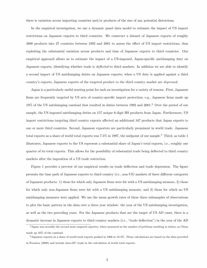
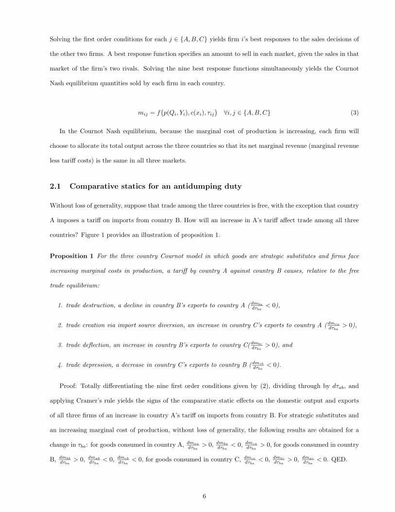
Without loss of generality, suppose that trade among the three countries is free, with the exception that country

A imposes a tariff on imports from country B. How will an increase in A’s tariff affect trade among all three

countries? Figure 1 provides an illustration of proposition 1.

Proposition 1 For the three country Cournot model in which goods are strategic substitutes and firms face

increasing marginal costs in production, a tariff by country A against country B causes, relative to the free

trade equilibrium:

1. trade destruction, a decline in country B’s exports to country A (dmba

dτba< 0),

2. trade creation via import source diversion, an increase in country C’s exports to country A (dmca

dτba> 0),

3. trade deflection, an increase in country B’s exports to country C(dmbc

dτba> 0), and

4. trade depression, a decrease in country C’s exports to country B (dmcb

dτba< 0).

Proof: Totally differentiating the nine first order conditions given by (2), dividing through by dτab, and

applying Cramer’s rule yields the signs of the comparative static effects on the domestic output and exports

of all three firms of an increase in country A’s tariff on imports from country B. For strategic substitutes and

an increasing marginal cost of production, without loss of generality, the following results are obtained for a

change in τba: for goods consumed in country A, dmaa

dτba> 0, dmba

dτba< 0, dmca

dτba> 0, for goods consumed in country

B, dmbb

dτba> 0, dmab

dτba< 0, dmcb

dτba< 0, for goods consumed in country C, dmcc

dτba< 0, dmbc

dτba> 0, dmac

dτba< 0. QED.

6

In this model, the existence of a deflected trade flow relies critically on the assumption of an increasing

marginal cost of production. Because firms equate the net marginal revenue of producing for each market in

equilibrium, anything that raises the cost of selling in one market will cause firms to reallocate their sales across

markets.

2.2 Comparative statics for a safeguard tariff

Without loss of generality, suppose that trade among the three countries is free, with the exception that country

A imposes a tariff on imports from countries B and C. Assume that the magnitudes of the tariffs set against B

and C are identical (τba = τca) and given by τ . How will an increase in country A’s tariff affect trade among

all three countries?

Proposition 2 For the three country Cournot model in which goods are strategic substitutes and firms face

increasing marginal costs in production, a tariff by country A against all other countries (B and C) causes,

relative to the free trade equilibrium:

1. trade destruction, a decline in country C and B’s exports to country A (dmba

dτ < 0, dmca

dτ < 0) and

2. two-way trade deflection, an increase in country B’s exports to country C(dmbc

dτ > 0) and an increase in

country C’s exports to country B(dmcb

dτ > 0).

Proof: Totally differentiating the nine first order conditions given by (2), dividing through by dτ , and

applying Cramer’s rule yields the signs of the comparative static effects of an increase in country A’s tariff on

imports from all countries on the domestic output and exports of all three firms. For strategic substitutes and

an increasing marginal cost of production, without loss of generality, the following results are obtained for a

change in τ : for goods consumed in country A, dmaa

dτ > 0, dmba

dτ < 0, dmca

dτ < 0, for goods consumed in country

B, dmbb

dτ > 0, dmab

dτ < 0, dmcb

dτ > 0, for goods consumed in country C, dmcc

dτ > 0, dmbc

dτ > 0, dmac

dτ < 0. QED.

Comparing a discriminatory antidumping policy and a nondiscriminatory safeguard, the theoretical model

predicts that two phenomena observed under an antidumping duty - trade creation via import source diversion

and trade depression - are absent under a safeguard. Because a safeguard creates an identical increase in

costs on products from both import sources, there is no incentive to favor one source over another. Thus, the

result that no trade is created through import source diversion is fairly obvious. With regard to the model’s

prediction of two-way trade deflection under a safeguard, the result is less obvious. For each country B and

C, the safeguard induces two conflicting forces of trade depression and trade deflection. Retained domestic

7

production that can no longer be sold in country A could “crowd out” imports and lead to trade depression,

but in the model this effect is swamped by each firm’s strong desire to export so that it will not be competing

against itself in its domestic market.

In the next section, we test the model’s predictions about trade deflection, trade depression, and two-way

trade deflection on a panel of Japanese product exports. Our approach is thus different from papers by Romalis

(2002) and Prusa (1997, 2001) who estimate empirical models of what we refer to as “trade destruction” and

“trade creation via import source diversion,”11 respectively.

3 Empirical Model and Estimation

3.1 The empirical investigation

The theoretical model presented in section 2 yields a number of predictions relating one country’s tariffs to trade

flows between foreign countries. Our empirical analysis focuses on the predictions of deflected, depressed and

two-way deflected trade for Japanese exports to 37 non-US trading partners. For clarity of exposition, ignoring

Japan’s 36 other trading partners, what does our theoretical model predict when the country imposing tariffs

is the US and the foreign countries are Japan and the EU? First, if the US imposes a country-specific tariff

against Japan in the form of an antidumping duty and imposes no tariff against the EU, the model predicts

deflected trade, an increase in Japanese exports to the EU. Second, if the US imposes a country-specific tariff

against the EU in the form of an antidumping duty, but not against Japan, the model predicts that Japanese

exports to the EU will fall, i.e., depressed trade. In this case, European exports that are diverted away from

the US market by the tariff and sold domestically within the EU depress imports from Japan. Third, if the

US imposes tariffs against both Japan and the EU in the form of a broadly-applied safeguard measure or two

simultaneously-imposed antidumping duties, the model predicts two-way deflected trade, a rise in Japanese

exports to the EU and in EU exports to Japan.12

3.2 Basic empirical model

To investigate the questions identified by the theoretical model, we develop the following reduced-form speci-

fication for the value of Japanese exports to country i based on equation (3):13

11More precisely, Romalis estimates the opposite effect - trade creation arising from the removal of a tariff.12We do not test for the rise in EU exports to Japan here as our analysis focuses on the response of Japanese exports only.13Unfortunately, only the value of imports is consistently available in the TRAINS data, so we cannot analyze the price and

quantity responses to a trade policy change separately.

8

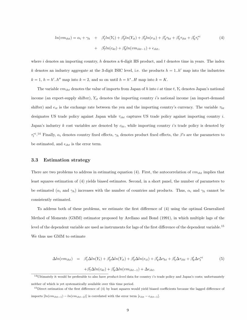
ln(vmiht) = αi + γh + β′1ln(Yt) + β′

2ln(Yit) + β′3ln(eit) + β′

4τht + β′5τiht + β′

6τ∗it (4)

+ β′7ln(ckt) + β′

8ln(vmiht−1) + εiht,

where i denotes an importing country, h denotes a 6-digit HS product, and t denotes time in years. The index

k denotes an industry aggregate at the 3-digit ISIC level, i.e. the products h = 1..h′ map into the industries

k = 1, h = h′..h′′ map into k = 2, and so on until h = h∗..H map into k = K.

The variable vmiht denotes the value of imports from Japan of h into i at time t, Yt denotes Japan’s national

income (an export-supply shifter), Yit denotes the importing country i’s national income (an import-demand

shifter) and eit is the exchange rate between the yen and the importing country’s currency. The variable τht

designates US trade policy against Japan while τiht captures US trade policy against importing country i.

Japan’s industry k cost variables are denoted by ckt, while importing country i’s trade policy is denoted by

τ∗it .14 Finally, αi denotes country fixed effects, γh denotes product fixed effects, the β’s are the parameters to

be estimated, and εiht is the error term.

3.3 Estimation strategy

There are two problems to address in estimating equation (4). First, the autocorrelation of vmiht implies that

least squares estimation of (4) yields biased estimates. Second, in a short panel, the number of parameters to

be estimated (αi and γh) increases with the number of countries and products. Thus, αi and γh cannot be

consistently estimated.

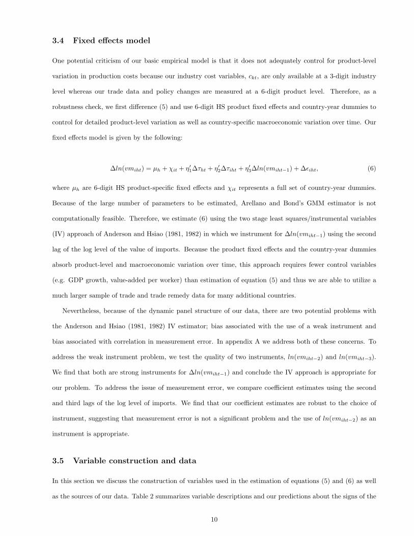
To address both of these problems, we estimate the first difference of (4) using the optimal Generalized

Method of Moments (GMM) estimator proposed by Arellano and Bond (1991), in which multiple lags of the

level of the dependent variable are used as instruments for lags of the first difference of the dependent variable.15

We thus use GMM to estimate

∆ln(vmiht) = β′1∆ln(Yt) + β′

2∆ln(Yit) + β′3∆ln(eit) + β′

4∆τht + β′5∆τiht + β′

6∆τ∗it (5)

+β′7∆ln(ckt) + β′

8∆ln(vmiht−1) + ∆εiht.

14Ultimately it would be preferable to also have product-level data for country i’s trade policy and Japan’s costs; unfortunately

neither of which is yet systematically available over this time period.15Direct estimation of the first difference of (4) by least squares would yield biased coefficients because the lagged difference of

imports [ln(vmiht−1)− ln(vmiht−2)] is correlated with the error term [εiht − εiht−1].

9

3.4 Fixed effects model

One potential criticism of our basic empirical model is that it does not adequately control for product-level

variation in production costs because our industry cost variables, ckt, are only available at a 3-digit industry

level whereas our trade data and policy changes are measured at a 6-digit product level. Therefore, as a

robustness check, we first difference (5) and use 6-digit HS product fixed effects and country-year dummies to

control for detailed product-level variation as well as country-specific macroeconomic variation over time. Our

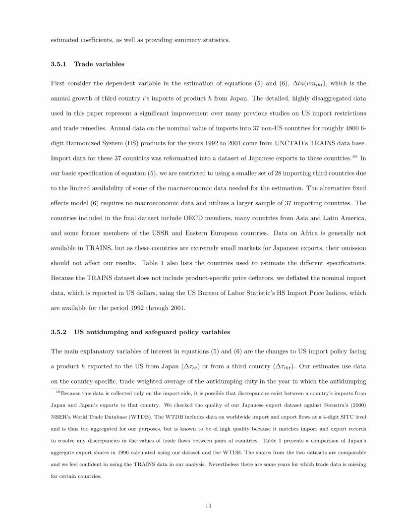
fixed effects model is given by the following:

∆ln(vmiht) = µh + χit + η′1∆τht + η′2∆τiht + η′3∆ln(vmiht−1) + ∆εiht, (6)

where µh are 6-digit HS product-specific fixed effects and χit represents a full set of country-year dummies.

Because of the large number of parameters to be estimated, Arellano and Bond’s GMM estimator is not

computationally feasible. Therefore, we estimate (6) using the two stage least squares/instrumental variables

(IV) approach of Anderson and Hsiao (1981, 1982) in which we instrument for ∆ln(vmiht−1) using the second

lag of the log level of the value of imports. Because the product fixed effects and the country-year dummies

absorb product-level and macroeconomic variation over time, this approach requires fewer control variables

(e.g. GDP growth, value-added per worker) than estimation of equation (5) and thus we are able to utilize a

much larger sample of trade and trade remedy data for many additional countries.

Nevertheless, because of the dynamic panel structure of our data, there are two potential problems with

the Anderson and Hsiao (1981, 1982) IV estimator; bias associated with the use of a weak instrument and

bias associated with correlation in measurement error. In appendix A we address both of these concerns. To

address the weak instrument problem, we test the quality of two instruments, ln(vmiht−2) and ln(vmiht−3).

We find that both are strong instruments for ∆ln(vmiht−1) and conclude the IV approach is appropriate for

our problem. To address the issue of measurement error, we compare coefficient estimates using the second

and third lags of the log level of imports. We find that our coefficient estimates are robust to the choice of

instrument, suggesting that measurement error is not a significant problem and the use of ln(vmiht−2) as an

instrument is appropriate.

3.5 Variable construction and data

In this section we discuss the construction of variables used in the estimation of equations (5) and (6) as well

as the sources of our data. Table 2 summarizes variable descriptions and our predictions about the signs of the

10

estimated coefficients, as well as providing summary statistics.

3.5.1 Trade variables

First consider the dependent variable in the estimation of equations (5) and (6), ∆ln(vmiht), which is the

annual growth of third country i’s imports of product h from Japan. The detailed, highly disaggregated data

used in this paper represent a significant improvement over many previous studies on US import restrictions

and trade remedies. Annual data on the nominal value of imports into 37 non-US countries for roughly 4800 6-

digit Harmonized System (HS) products for the years 1992 to 2001 come from UNCTAD’s TRAINS data base.

Import data for these 37 countries was reformatted into a dataset of Japanese exports to these countries.16 In

our basic specification of equation (5), we are restricted to using a smaller set of 28 importing third countries due

to the limited availability of some of the macroeconomic data needed for the estimation. The alternative fixed

effects model (6) requires no macroeconomic data and utilizes a larger sample of 37 importing countries. The

countries included in the final dataset include OECD members, many countries from Asia and Latin America,

and some former members of the USSR and Eastern European countries. Data on Africa is generally not

available in TRAINS, but as these countries are extremely small markets for Japanese exports, their omission

should not affect our results. Table 1 also lists the countries used to estimate the different specifications.

Because the TRAINS dataset does not include product-specific price deflators, we deflated the nominal import

data, which is reported in US dollars, using the US Bureau of Labor Statistic’s HS Import Price Indices, which

are available for the period 1992 through 2001.

3.5.2 US antidumping and safeguard policy variables

The main explanatory variables of interest in equations (5) and (6) are the changes to US import policy facing

a product h exported to the US from Japan (∆τht) or from a third country (∆τiht). Our estimates use data

on the country-specific, trade-weighted average of the antidumping duty in the year in which the antidumping16Because this data is collected only on the import side, it is possible that discrepancies exist between a country’s imports from

Japan and Japan’s exports to that country. We checked the quality of our Japanese export dataset against Feenstra’s (2000)

NBER’s World Trade Database (WTDB). The WTDB includes data on worldwide import and export flows at a 4-digit SITC level

and is thus too aggregated for our purposes, but is known to be of high quality because it matches import and export records

to resolve any discrepancies in the values of trade flows between pairs of countries. Table 1 presents a comparison of Japan’s

aggregate export shares in 1996 calculated using our dataset and the WTDB. The shares from the two datasets are comparable

and we feel confident in using the TRAINS data in our analysis. Nevertheless there are some years for which trade data is missing

for certain countries.

11

measure was imposed.17 For a product h, we examine the effect of (1) the imposition of a US antidumping duty

against Japan, (2) the imposition of a US antidumping duty against a third country i, and (3) the imposition of

a US safeguard policy. As discussed in section 2, the theoretical model predicts that the sign of the coefficient

on (1) is positive, on (2) is negative, and on (3) is positive.18

We collected data on the US imposition of country-specific antidumping duties and safeguard measures

at the 6-digit HS level over the 1992 through 2001 period from a variety of US government publications,

most notably the Federal Register. For antidumping and safeguard cases filed during the sample, we obtained

the names and 6-digit HS codes for the products involved, the outcome of the case (affirmative, negative, or

terminated, as well as the type of measure for safeguards), the names of the countries that faced the import

restrictions, the trade-weighted average duty when duties were imposed, and, most importantly, the date a

case was initiated and the date a trade restriction began.19 For the antidumping policies, we interact a variable

indicating that the policy was imposed in year t with the level of the antidumping duty that is imposed, to

help control for the heterogeneity in duties imposed across exporters and across investigations. On the other

hand, we use a simple indicator variable to examine the safeguard policies, due to the fact that sometimes the

safeguard measure is imposed as a quantitative restriction or a tariff-rate quota, as opposed to a simple ad

valorem duty.17The duty data was generously provided by Bruce Blonigen and his AD website

http://darkwing.uoregon.edu/ bruceb/adpage.html .18We do not investigate the impact on Japanese exports of US AD (or SG) investigations that do not result in duties, but

which are terminated or settled. While such an investigation could lend further insight into the overall impact of Staiger and

Wolak’s (1994) “investigation effect,” “suspension effect” and “withdrawal effect,” of the non-duty impact of AD investigations, it

is beyond the scope of issues under investigation here and thus we leave it to future research. Furthermore, while the theoretical

model also generates predictions on the expected impact of the removal of trade remedies, we do not report estimates of those

impacts here. The primary issue is the quality of the antidumping policy removal data. We are primarily concerned with

measurement error as it is difficult to “time” when an antidumping measure is removed, given that in many cases the removal is

applied retroactively (with the refunding of duties), but in a manner which could not have been reasonably anticipated by the

exporters. Nevertheless, we do note that the estimates (available from the authors upon request) for our policy variables of interest

are not significantly altered with the inclusion of the policy removal variables.19To clarify the timing of our different variables, the variables ∆ AD Dutyjpn,ht and ∆ AD Dutyiht are nonzero in the period

in which the investigation into an antidumping case that results in a duty is begun. The ∆ SG Policyht variable is an indicator

that is equal to 1 in the period in which a safeguard measure goes into effect. This reflects the fact that in AD cases the targeted

exporters begin to respond to provisional antidumping duties that are imposed shortly after the date the investigation is announced.

Safeguard cases, on the other hand, have a very uncertain outcome and almost never use temporary trade restrictions during the

investigation phase.

12

3.5.3 Macroeconomic variables

We include controls for growth in the exporting (∆ln(Yt)) and importing countries’ GDP (∆ln(Yit)), growth of

the real yen/country i currency exchange rate (∆ln(eit)), and proxies for changes in the importing countries’

trade policies (∆τ∗it ).

We expect an increase in the GDP growth of the exporting country (Japan) to lead to a fall in Japanese

export growth because domestic demand for the export goods will be higher. In other words, Japan is expected

to export domestic weakness. Second, in terms of currency changes, export growth should be higher when the

yen is weakening relative to the importing country’s currency. Thus, we expect a positive sign on the coefficient

for growth of the real exchange rate.

For the importing country, an increase in GDP growth should be associated with higher Japanese export

growth. To proxy for changes to an importing country’s overall trade policy that we cannot observe, for example,

an across the board tariff reduction or a reduction in the administrative cost of exporting to a particular

importing country, we control for changes in an importing country’s “openness.” Openness is defined as the

sum of real aggregate imports and exports divided by real GDP. For some countries, real aggregate import

and export series were not available. For these countries, we calculated “openness” using the corresponding

nominal variables. We believe that an increase in this variable is associated with liberalization of country i’s

trade policy, and thus, expect a positive sign on its coefficient.

Data on real GDP, real aggregate imports, and real aggregate exports come from two sources: the OECD

Main Economic Indicators and the IMF’s International Financial Statistics (IFS). Whenever possible, we used

the OECD data to construct the macroeconomic controls. When OECD data were not available or were only

available for a short timespan, we used data from the IFS. We construct real bilateral Japanese Yen to country

i currency rates for 20 countries using data supplied by the USDA Economic Research Service. An increase in

the value of the real exchange rate implies an appreciation of country i’s currency. For Norway and Switzerland,

bilateral rates were not available from USDA so we use real exchange rate indices from the IFS.20

3.5.4 Industry-level variables

Lastly, we use two measures of productivity changes for Japanese manufacturing industries: the growth of the

average wage and the growth of value-added per worker. This addresses a concern that our policy variables20For the IFS series, an increase in the value of the real exchange rate index implies a real appreciation of the Norwegian and

Swiss currencies, respectively. We thank Matthew Shane of the ERS of the USDA for providing us with the data and answering

questions about the construction of the USDA’s real exchange rates.

13

may not be measuring true treatment effects, but may be picking up the effect of an omitted variable - like a

Japanese productivity improvement - that would be associated with the imposition of a US import barrier on

Japanese imports and an increase in Japanese export growth to other countries. We expect the sign on both

productivity measures to be positive.

Japanese manufacturing industry data at the 3-digit ISIC (Rev. 2) level for the years 1992-1999 came from

the UNIDO (2002). We used data on number of employees, value-added and average wages to construct two

productivity measures: the growth of value-added per worker and the growth of average wages.

4 Empirical Results

4.1 Estimation results using the GMM procedure

Table 3 presents our estimates of equation (5) using the Arellano and Bond (1991) GMM estimator. Speci-

fications (1) and (2) present estimates on the full set of industries (agricultural and manufacturing) over the

1992-2001 period thus leaving out the industry-level controls. Specifications (3) through (5) present estimates

for all manufacturing industries from 1992-1999, all years for which the ISIC industry variables are available.

Consider first specification (1) and our estimates for the policy variables of interest, which provide evidence

in support of some of the key predictions of our theoretical model. US imposition of antidumping measures

against Japan is associated with statistically significant deflection of Japanese exports to third country markets,

and US imposition of antidumping measures against third countries is associated with a statistically signifi-

cant depression of Japanese exports to those markets. Interestingly, the coefficient estimate on the safeguard

indicator variable also implies that a safeguard policy is associated with a statistically significant depression of

Japanese exports to third markets.

With respect to the size of the estimates, specification (1) indicates that the imposition of a 1% antidumping

duty against Japanese exports of product h (but not exporters from country i) is associated with an 0.14%

increase in Japanese exports of h to country i. To understand the magnitude of the effect, consider that the

median antidumping duty (conditional on a duty being imposed) facing a Japanese exporter in the sample is

37.13%, which implies a 5.24% average increase in Japanese exports of h to an importing country i. In the

next section we investigate whether the magnitude of the trade deflection effect facing Japanese exports varies

substantially across some of its particularly important trading partners i as well important product categories

of h.

14

On the other hand, the imposition of a 1% antidumping duty against the third country i’s exporters, but

not against Japan, is associated with a 1.269% reduction in Japanese exports of that same product h to country

i. This is consistent with the idea that when the output produced by firms in country i cannot be sold in the

US, but is sold domestically, it depresses (crowds out) country i’s imports of the same product from Japan.

With the median duty facing a country i’s exports of h being 14.84% in this particular sample of data, this

translates into an 18.83% average reduction in Japanese exports to a third country, which is also a significant

effect.

Finally, and perhaps surprisingly, the US imposition of an MFN safeguard policy also has a strong trade

depressing effect. After using the Kennedy (1981) formula to convert the coefficient estimate for the dummy

variable to its marginal effects interpretation, the imposition of a US SG on an HS product implies a 67%

reduction in Japanese exports of that product to country i.21

Next, the coefficient estimates in specification (1) for the macroeconomic and “openness” control variables

also have the predicted sign. Since they are not of particular interest to our investigation and are fairly robust

across specifications, we will omit a substantive discussion of them here.

In specifications (2) through (4) of table 3, we sequentially consider additional control variables as one

way to check the sensitivity of our results. Overall, the estimates on the policy variables of interest appear

robust to changes in model specification. For example, the estimated impacts of the growth in the values

of the Yen/country i exchange rate, which we add in specification (2), is positive as predicted by the theory.

Nevertheless, we do lose a substantial number of observations from the sample when we add in the real exchange

rate variable.

More importantly, in specifications (3) and (4) we add industry-level (ISIC 3-digit) control variables (avail-

able from 1992-1999). Because our results for the policy variables are robust to the inclusion of industry level

controls, we believe that the policy variables are likely capturing the true treatment effect of the policy. Unfor-

tunately, because the industry variables are only available for manufacturing industries between 1992 and 1999,

we also lose a number of observations in these specifications. Specification (5) shows that the small changes

to the estimates for the policy variables of interest (the slight increase in the size of the AD duty imposition

21While safeguard measures often include exemptions for free-trade partners and developing countries, in our sample, safeguard

measures were applied quite broadly to almost all US import sources. The correlation coefficient between changes in US safeguard

policy against Japan - the variable in our estimation - and against all other countries was 0.73. In contrast, there was considerably

more variation in the application of antidumping duties. The correlation coefficient between changes in US antidumping policy

against Japan and against all other countries was only 0.24.

15

variables and decrease in the statistical significance of the SG policy imposition variable) are most likely due to

the loss of observations from years 2000 and 2001. For the case of the safeguard variable in particular, this is

likely due to the variation generated by the observations surrounding the 2000 US safeguard policy on circular

welded pipe that particularly affected global pipe trade from and into markets such as Korea, Japan and the

EU.22

At the bottom of table 3 we also report the z-statistic on the average autocovariance in residuals of order

2 for specifications (1) through (5). For all specifications, we are able to reject the hypothesis of second order

autocovariance in the residuals, which leads us to conclude that our Arellano and Bond GMM estimator yields

consistent parameter estimates. In all of the specifications reported in (1) through (5) we include two lags of

the dependent variable, as we found that inclusion of a second lag improved the fit of the model and yet did

not significantly change our parametric estimates.

Finally, specification (6) presents a final robustness check on the results in table 3. Using the sample from

specification (1), we estimate the fixed effects specification of equation (6) with the Anderson and Hsiao (1981,

1982) instrumental variables technique, as described in section 3.4. The results in specification (6) are broadly

consistent with those in specifications (1) - (5). The estimated impact of a 0.127% increase in exports in

response to a 1% increase in the US antidumping duty against Japan falls within the 95% confidence intervals

of the estimated coefficients in specifications (1) - (5), but is not significantly different from zero. We will show

in the next section, however, this result appears to be driven by the particular sample of countries and years

available in the data set required for the GMM estimation.

To summarize the results of table 3, we find first that the US imposition of an AD duty against Japan

leads to a deflection of Japanese trade to third markets (row 1): Japanese exports to third markets increase

by estimates ranging from 0.127% to 0.168% for each 1% increase in the US duty. Second, the US imposition

of an AD duty against a third country is associated with the depression of Japanese exports to those third

markets (row 2): Japanese exports to third markets fall by 0.870% to 1.292% for each 1% increase in the duty.

Third, the US imposition of a broadly applied SG measure against Japan and other exporting countries leads

to a depression of Japanese trade to third markets (row 3): Japanese exports to third markets fall by 63% to

70%.22Korea was the largest exporter adversely affected by the US policy, so much so that it contested the measure through a formal

WTO trade dispute. It is therefore likely that because of a glut of Korean pipe being retained domestically, Japanese exports of

pipe to Korea were depressed in 2000, thus driving the significance of the safeguard results in specifications in which the year 2000

data is included.

16

Even though the trade depressing effect of a US safeguard measure is statistically significant, we are con-

cerned about the robustness of this particular result. While there were hundreds of US AD measures imposed

over the 1992-2001 period, there were only five US SG investigations which resulted in the imposition of defini-

tive measures (tariffs, quotas or tariff-rate quotas). Even though each of the SG measures may affect more than

one 6-digit HS category, we are nevertheless concerned about the relatively few number of safeguard observa-

tions in the estimation. This concern is further driven by the fact that some US safeguard measures covered

products (e.g., brooms, lamb meat, wheat gluten) which were not of substantial importance to Japanese ex-

porters. Nevertheless, our results with regard to the imposition of a safeguard measure do reject our theoretical

model’s prediction of two-way trade deflection.

4.2 IV estimates using fixed effects from an expanded sample of data

As described in section 3.4, an advantage to using the fixed effects model and instrumental variables estimation

procedure is that it does not require macroeconomic and industry controls. Thus, we can estimate the model

using a significantly larger sample of trade data.23 Therefore, in table 4 we provide a set of estimation results

using data on Japanese exports to all of the countries listed in table 1 except the US. When compared to the

sample of specification (6) of table 3, for example, this adds to the estimation sizable import markets such

as Taiwan, China, Singapore and the Philippines, in addition to requiring one fewer lag of the dependant

variable in the estimation, providing effectively another year (1994) of trade remedy data. Together, these

elements add roughly 113,000 observations. Estimates of the coeffcients on the policy variables are consistent

with our findings of trade deflection and trade depression reported in table 3. In Appendix A we formally

describe the tests we perform on the strength of our instrumental variables. Because F-tests confirm that all of

our instrumental variables are strong instruments, we conclude that our instrumental variables estimates are

unbiased.

Specification (7) of table 4 presents the baseline IV specification for comparison with the results of table 3.24

The estimates for trade deflection and trade depression are statistically significant on this larger sample of

data. The primary change in results from table 3 relates to the size of the coefficient estimate on the trade

depression effect of an antidumping duty against country i, as it falls from -1.271 in specification (1) to -0.281

in specification (7).

Nevertheless, to better interpret and compare the magnitude of the estimates, consider table 5. The first23The results presented in table 4 use country-year dummies and 6-digit HS product fixed effects.24Note that specification (10) presents the biased OLS estimates as a benchmark for comparison.

17

column presents the median duty, conditional on a duty being applied, for the sample of 141,164 observations

used in specifications (1) - (6). The second column presents the median duty, conditional on a duty being

applied, for the sample of 254,074 observations used in specifications (7) -(10). The third column quantifies

the effect of imposing a typical duty, in this case, the conditional median25 using the coefficient estimated from

specification (1). The fourth and fifth columns similarly quantify the effect of imposing a typical duty using the

coefficient estimates from specifications (7) and (8). First, comparing our estimates from specifications (1) and

(7), we see that the magnitudes of the trade deflection effect in the two samples, using two different econometric

specifications, is similar. In our GMM specification (1), imposing the conditional median duty is associated

with a roughly 5% increase in Japanese exports of that product to third countries while for our IV specification

(7), imposing the conditional median duty is associated with a roughly 7% increase in Japanese exports. There

is, however, a noticeable difference in the magnitude of the trade depression effect between specifications (1)

and (7). The depression effect associated with the conditional median in the GMM specification (1) of a 19%

fall in Japanese exports to country i is considerably larger than that in the IV specification (7) of a 5% fall in

Japanese exports. We believe this difference in the magnitude of trade depression is likely due to differences

in the underlying sample of data. In particular, the GMM sample requiring macroeconomic data does not

contain observations for a number of Japan’s sizable export markets, including China, Taiwan, Singapore and

the Philippines. Furthermore, the GMM procedure also requires an additional lag of the trade data, and the

result for those specifications is to lose all useful trade remedy variation taking place in 1994.

Thus, in specification (8) of table 4 we explore the question of whether there are substantial differences

in trade deflection and trade depression effects for Japanese exports across importing country markets. This

specification is estimated on the identical sample of data as specification (7), but in this column we present

estimates where we interact the antidumping variables of interest with a number of importing country indica-

tors, examining the variation across some of Japan’s important import markets. This approach yields strong

evidence of trade deflection, for example, associated with Japan’s exports to both the EU and Korea, which

is quite intuitive, given that they are the two largest destination markets for Japanese exports in the sample

(see again table 1). These two countries are thus likely to be the “next best” alternative markets for Japanese

exports that get shut out of the US because of a US trade policy. Table 5 further illustrates the significance of

the economic magnitude of Japan’s trade deflection to the EU and Korea, as the median duty imposed against25In all our samples, the mean duty conditional on a duty being imposed is larger than the median. Thus, when we use the

conditional mean duty as a typical duty to quantify the magnitudes of trade deflection and trade depression, the results are slightly

(1-5 percentage points) larger.

18

products which the Japanese export to these countries results in a 16% increase in Japanese exports to the EU

and a 20% increase in Japanese exports to Korea. This is considerably larger than the roughly 7% increase in

Japanese exports to countries other than the EU, Korea, China, and India.

Turning to the country-specificity of trade depression, specification (8) of table 4 indicates that US an-

tidumping duties on third countries are associated with statistically significant reduction in Japanese exports

to China and India. Table 5 illustrates the economic significance of these results as well, quantifying an 81%

decrease in Japanese exports to India and a 30% decrease in Japanese exports to China associated with the im-

position of median US antidumping duties against each of these two countries. We believe that the magnitude

and significance of trade depression for India and China in particular may be related to three phenomena. First,

the second column of table 5 indicates that both of these countries face extremely high US antidumping duties:

the median duty imposed against Chinese exports to the US was 121% while the median duty against Indian

exports was 72%. It seems likely that duties facing these two countries are frequently prohibitive, which would

create a severe glut of the affected products in the Chinese and Indian markets which could crowd out imports

from Japan and lead to a sizable amount of trade depression. Second, unlike a number of other importing

countries in the sample, China and India are also frequent targets of US antidumping activity. And finally,

even beyond a higher frequency of being targeted, both of these countries are also less frequently targeted

alongside Japan in a multi-country US AD investigation over the same product (i.e., relative to the EU and

Korea, whose exporters have a higher frequency of being alongside Japan in a multi-country US AD investiga-

tions over the same product). This variation likely allows for more precise estimation of the trade depressing

effect associated with a US antidumping duty being applied on third countries such as China and India alone

(i.e., not simultaneously with Japan). This is also a potential explanation for the imprecisely estimated trade

depressing effects of US antidumping toward the EU and Korea in specification (8) of table 4.

4.3 IV estimates for steel versus non-steel products

Another question to consider is whether the AD or SG measures associated with the US steel industry are

particularly important in our results, given that this industry is the most frequent user of US trade remedies.26

To address this issue, in specification (9) of table 4 we separate out the estimated policy effects for steel and

non-steel products by interacting each policy variable of interest with an indicator for whether the underlying

6-digit HS product was a steel (HS chapter 72 or 73) or non-steel product. With the exception of the estimates

26For example, for the 1992-2001 period, over 50% of US AD investigations that resulted in duties affected steel imports.

19

for the SG policy (which again are tested on a relatively small number of policy actions), the estimates suggest

that the trade deflection and trade depression results may be even stronger for non-steel products than the steel

products that have traditionally been the most active targets of US trade remedy laws. This is particularly

important, given the likelihood that any future growth in use of US trade remedies is likely to come from

non-steel industries as they learn from the steel industry’s experience. Thus this table might suggest that

future use of trade remedies may lead to even more trade deflection and trade depression.

4.4 Specification tests

As a final check on our results, we conduct a specification test on our GMM (5) and IV-fixed effects (6) econo-

metric models. These results are reported in Table 6. The thought experiment is similar to that conducted in

the labor literature, beginning with Ashenfelter (1978), on the evaluation of training programs for unemployed

workers. As applied to our context, we investigate whether the imposed policy (i.e., an AD duty) can be used

to predict the change in the dependent variable that occurred before the policy was imposed. Specifically, we

might be concerned that a Japanese, product-level cost shock in t− 1 led to an increase in Japanese exports to

US and non-US markets in t − 1, and thus that the US policy response in t could actually be used to predict

the t − 1 export growth to importing countries i. If this were the case, our model could be misspecified and

what we claim to be trade deflection might just be an increase in Japanese exports associated with a favorable

cost shock to a particular product exported to many different markets.

To investigate this question we therefore regress lagged (t − 1) product-level Japanese export growth to

country i on period t US policy changes and other explanatory variables.27 If the coefficient on a US policy

change in t were positive and statistically significant, the imposition of the US AD policy could be interpreted

as a predictor of higher than normal Japanese export growth of that product to all markets in t− 1 which, in

turn, might have been due to a cost shock. Similarly, if US imposition of an AD duty against country i in t

were a statistically significant predictor of a reduction in Japanese exports to i in t− 1, this could suggest that

a product-level cost shock in the importing country was behind what we have described as “trade depression.”

Nevertheless, in all specifications in table 6, the coefficients on changes in US AD policies against Japan and

country i are not statistically significant. Our results indicate that the model is correctly specified and that

the policy variables are measuring the true treatment effect of a policy change.27Due to the small number of changes in safeguards policy, there were insufficient observations to perform this specification test

using safeguards.

20

5 Conclusion

This paper empirically examines whether a country’s use of an import-restricting trade policy distorts a foreign

country’s exports to third markets. To investigate this question we match data on US use of antidumping and

safeguard trade remedies over the 1992-2001 period to Japanese product-level exports to third countries. We

find evidence that US trade remedies both deflect and depress Japanese exports. The median antidumping

duty against Japan leads to a 5-7% average increase in Japanese exports to a non-US trading partner. When

the median US antidumping duty is imposed against a third country’s exporters, Japanese exports in the same

product to that third country decrease by an average of 5-19%. Finally, when faced with a US safeguard

measure, Japanese exports to third countries fall by somewhere between 55% and 70%. Our results on the

“deflection” and “depression” of Japanese exports vary substantially (and in intuitively appealing ways) across

importing countries, and the estimated impact appears stronger for non-steel relative to steel products.

There are some limitations of our results and approach. First, we have focused on the export response

of only one US trading partner. An open research question is whether US trade policy similarly distorts the

exports of other trading partners, including developing countries. We speculate, for example, that the ability of

developing countries to deflect trade may be more limited than that of a country like Japan. Furthermore, we

are less confident in our results regarding the impact of safeguard policies, as there are relatively few safeguard

observations in our dataset.

Nevertheless, our results have implications for the empirical literature on the impact of trade policy decisions

made by “large” countries, defined as those that are able to affect exporters’ prices. For example, Chang and

Winters (2002) use similarly disaggregated, product level data on unit values and tariffs for Brazil and its

trading partners and find that the creation of MERCOSUR was accompanied with a substantial decline in

the prices of non-member exporters to the region. While we do not test whether any of the countries in our

analysis are “large” in the sense of their ability to affect the prices of foreign exporters, we provide evidence

that the US’s trade policy decisions do impact the export behavior of a particularly important trading partner.

Finally, we speculate that the results of this paper suggest an additional explanation for the proliferation

of antidumping laws around the world (Miranda et al., 1998; Prusa, 2001) that has not previously been inves-

tigated. Much of the prior literature commenting on this proliferation has focused on the retaliation argument:

countries adopt trade remedy laws in order to establish a credible retaliatory threat that will discourage for-

eign trade remedies targeted against their exporters (Prusa and Skeath, 2002; Blonigen and Bown, 2003). Our

results indicate that the imposition of a US trade remedy can lead to a substantial export surge to a third

21

country’s market. This third country may therefore face pressure of its own to respond with a trade remedy.

Therefore, US actions may induce trade policy actions by third country importers in addition to (and that is

separate from) retaliation-based trade policy actions. While we do not test here for the formal link between

US trade policy actions and responses by the governments of third countries facing deflected trade, our results

that associate substantial export surges with US trade policy changes suggests an additional explanatory factor

that should be an area of future research.

Acknowledgements

We thank Robert Staiger, Bruce Blonigen, Andrew Bernard, Matt Slaughter, Tom Prusa, Steve Redding,

James Tybout, Jeff Campbell, Eric French, Dan Sullivan, Rachel McCulloch, Jay Shambaugh, Matthew Shane

and seminar participants at the 2004 NBER ITI Summer Institute, the 2003 MWIEG Spring meetings, the

2003 NASMES meetings, the 2003 ETSG meetings, the 2003 Federal Reserve SCIEA Fall meetings, Brandeis

University, Dartmouth College, the Federal Reserve Bank of Chicago, University of Maryland and American

University for helpful comments on an early version of the paper. Jaimie Lien provided outstanding research

assistance. Bown acknowledges financial support from a Mazer Award and Perlmutter Fellowship at Brandeis

University, as well as the Okun-Model Fellowship at the Brookings Institution. The opinions expressed in this

paper are those of the authors and do not necessarily reflect those of the Federal Reserve Bank of Chicago or

the Federal Reserve System. All remaining errors are our own.

22

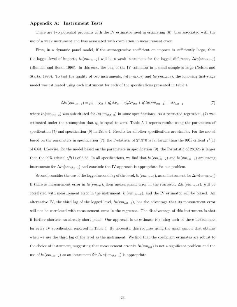
Appendix A: Instrument Tests

There are two potential problems with the IV estimator used in estimating (6); bias associated with the

use of a weak instrument and bias associated with correlation in measurement error.

First, in a dynamic panel model, if the autoregressive coefficient on imports is sufficiently large, then

the lagged level of imports, ln(vmiht−2) will be a weak instrument for the lagged difference, ∆ln(vmiht−1)

(Blundell and Bond, 1998). In this case, the bias of the IV estimator in a small sample is large (Nelson and

Startz, 1990). To test the quality of two instruments, ln(vmiht−2) and ln(vmiht−3), the following first-stage

model was estimated using each instrument for each of the specifications presented in table 4.

∆ln(vmiht−1) = µh + χit + η′1∆τht + η′2∆τiht + η′3ln(vmiht−2) + ∆εiht−1, (7)

where ln(vmiht−3) was substituted for ln(vmiht−2) in some specifications. As a restricted regression, (7) was

estimated under the assumption that η3 is equal to zero. Table A-1 reports results using the parameters of

specification (7) and specification (9) in Table 4. Results for all other specifications are similar. For the model

based on the parameters in specification (7), the F-statistic of 27,370 is far larger than the 99% critical χ2(1)

of 6.63. Likewise, for the model based on the parameters in specification (9), the F-statistic of 28,025 is larger

than the 99% critical χ2(1) of 6.63. In all specifications, we find that ln(vmiht−2) and ln(vmiht−3) are strong

instruments for ∆ln(vmiht−1) and conclude the IV approach is appropriate for our problem.

Second, consider the use of the logged second lag of the level, ln(vmiht−2), as an instrument for ∆ln(vmiht−1).

If there is measurement error in ln(vmiht), then measurement error in the regressor, ∆ln(vmiht−1), will be

correlated with measurement error in the instrument, ln(vmiht−2), and the IV estimator will be biased. An

alternative IV, the third lag of the logged level, ln(vmiht−3), has the advantage that its measurement error

will not be correlated with measurement error in the regressor. The disadvantage of this instrument is that

it further shortens an already short panel. Our approach is to estimate (6) using each of these instruments

for every IV specification reported in Table 4. By necessity, this requires using the small sample that obtains

when we use the third lag of the level as the instrument. We find that the coefficient estimates are robust to

the choice of instrument, suggesting that measurement error in ln(vmiht) is not a significant problem and the

use of ln(vmiht−2) as an instrument for ∆ln(vmiht−1) is appropriate.

23

References

[1] Anderson, T.W., Hsiao, C., 1981. Estimation of Dynamic Models with Error Components. Journal of the

American Statistical Association 76, 598-606.

[2] Anderson, T.W., Hsiao, C., 1982. Formulation and Estimation of Dynamic Models Using Panel Data.

Journal of Econometrics 18, 47-82.

[3] Arellano, M., Bond, S., 1991. Some Tests of Specification for Panel Data: Monte Carlo Evidence and an

Application to Employment Equations. Review of Economic Studies 58, 277-297.

[4] Ashenfelter, O., 1978. Estimating the Effect of Training Programs on Earnings. Review of Economics and

Statistics 60, 47-57.

[5] Bagwell, K., Staiger, R.W., 1997. Multilateral Tariff Cooperation during the Formation of Free Trade

Areas. International Economic Review 38, 291-319.

[6] Bagwell, K., Staiger, R.W., 1999. An Economic Theory of GATT. American Economic Review 89, 215-248.

[7] Bagwell, K., Staiger, R.W., 2004. Multilateral Trade Negotiations, Bilateral Opportunism and the Rules

of GATT/WTO. Journal of International Economics 63, 1-29.

[8] Blundell, R., Bond, S., 1998. Initial Conditions and Moment Restrictions in Dynamic Panel Data Models.

Journal of Econometrics 87, 115-143.

[9] Blonigen, B.A., Prusa, T.J., 2004. Antidumping. in: Harrigan, J., Choi, E.K., (Eds.), Handbook of

International Trade, Vol. I. Blackwell, Oxford, pp. 251-284.

[10] Blonigen, B.A., Bown, C.P., 2003. Antidumping and Retaliation Threats. Journal of International Eco-

nomics 60, 249-273.

[11] Bown, C.P., Crowley, M.A., 2005. Safeguards. in: Macrory, P., Appleton, A., Plummer, M. (Eds.), The

World Trade Organization, Legal, Economic and Political Analysis, Vol. II. Springer, Dordrecht, pp. 43-66.

[12] Bond, E.W., Syropolous, C., 1996. The Size of Trading Blocs: Market Power and World Welfare Effects.

Journal of International Economics 40, 411-437.

[13] Chang, W., Winters, L.A., 2002. How Regional Blocs Affect Excluded Countries: The Price Effects of

MERCOSUR. American Economic Review 92, 889-904.

24

[14] Clausing, K.A., 2001. Trade Creation and Trade Diversion in the Canada - United States Free Trade

Agreement. Canadian Journal of Economics 34, 677-696.

[15] Ethier, W.J., 2004. Political Externalites, Nondiscrimination, and a Multilateral World. Review of Inter-

national Economics 12, 303-320.

[16] European Union., 2002. Proposed EU Steel Safeguard Measures. Press release MEMO/02/67, 25 March.

[17] Feenstra, R.C., 2000. World Trade Flows, 1980-1997, with Production and Tariff Data. UC-Davis, mimeo

(and accompanying CD-Rom).

[18] Gallaway, M.P., Blonigen, B.A., Flynn, J.E., 1999. Welfare Costs of the US Antidumping and Counter-

vailing Duty Laws. Journal of International Economics 49, 211-244.

[19] Horn, H., Mavroidis, P., 2001. Economic and Legal Aspects of the Most-Favored Nation Clause. European

Journal of Political Economy 17, 233-279.

[20] International Monetary Fund, 2003. International Financial Statistics, Database and Browser CD-Rom.

[21] Kennedy, P.E., 1981. Estimation with Correctly Interpreted Dummy Variables in Semilogarithmic Equa-

tions. American Economic Review 71, 801.

[22] Krishna, P., 2004. The Economics of Preferential Trade Agreements. in: Choi, E.K., Hartigan, J. (Eds.),

Handbook of International Trade, Vol. II: Economic and Legal Analyses of Trade Policy and Institutions,

Blackwell, Oxford.

[23] Levy, P., 1997. A Political-Economic Analysis of Free-Trade Agreements. American Economic Review. 87,

506-519.

[24] McLaren, J.E., 2002. A Theory of Insidious Regionalism. Quarterly Journal of Economics CXVII, 571-608.

[25] Miranda, J., Torres, R.A., Ruiz, M., 1998. The International Use of Antidumping: 1987-1997. Journal of

World Trade 32, 5-71.

[26] Nelson, C.R., Startz, R., 1990. Some Further Results on the Exact Small Sample Properties of the Instru-

mental Variable Estimator. Econometrica 58, 967-976.

[27] Organization for Economic Cooperation and Development, 2002. OECD Main Economic Indicators.

25

[28] Prusa, T.J., 1997. The Trade Effects of US Antidumping Actions. in: Feenstra, R.C. (Ed.), The Effects of

US Trade Protection and Promotion Policies. University of Chicago Press, Chicago.

[29] Prusa, T.J., 2001. On the Spread and Impact of Anti-Dumping. Canadian Journal of Economics 34,

591-611.

[30] Prusa, T.J., Skeath, S., 2002. The Economic and Strategic Motives for Antidumping Filings.

Weltwirtschaftliches Archiv 138, 389-413.

[31] Romalis, J., 2002. NAFTA’s and CUSFTA’s Impact on North American Trade. University of Chicago -

GSB mimeo, July.

[32] Staiger, R.W., Wolak, F.A., 1994. Measuring Industry Specific Protection: Antidumping in the United

States. Brookings Papers on Economic Activity: Microeconomics, 51-118.

[33] United Nations Industrial Development Organization, 2002. Industrial Statistics Database: 3-digit level

of ISIC Code (Rev. 2) CD-Rom.

[34] United Nations Conference on Trade and Development, various issues. Trade Analysis and Information

System (TRAINS) CD-Rom.

[35] United States Department of Agriculture (Economic Research Service), 2005. International Macroeconomic

Dataset. available on-line at http://www.ers.usda.gov/Data/macroeconomics/.

[36] Viner, J., 1950. The Customs Union Issue. Carnegie Endowment for International Peace, New York.

[37] WTO, 2002. Report (2002) of the Committee on Safeguards to the Council for Trade in Goods. available

on-line at http://www.wto.org/, document number G/L/583, 4 November.

[38] WTO, 2003. Report (2003) of the Committee on Safeguards to the Council for Trade in Goods. available

on-line at http://www.wto.org/, document number G/L/651, 24 October.

26

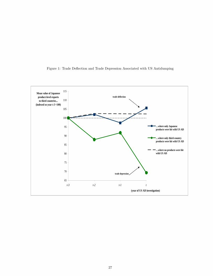
Figure 1: Trade Deflection and Trade Depression Associated with US Antidumping

65

70

75

80

85

90

95

100

105

110

115

t-3 t-2 t-1 t

Mean value of Japanese product-level exportsto third countries...

(indexed so year t-3 =100)

…where only Japaneseproducts were hit with US AD

…where only third-countryproducts were hit with US AD

…where no products were hitwith US AD

(year of US AD investigation)

trade depression

trade deflection

27

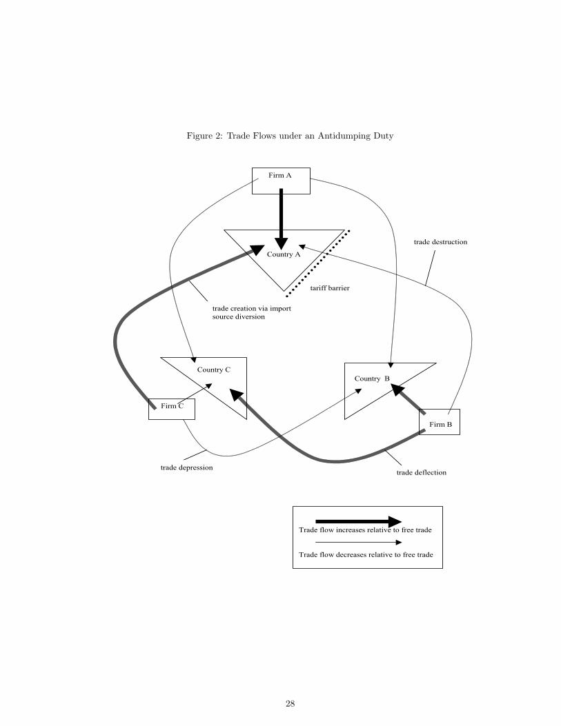
Figure 2: Trade Flows under an Antidumping Duty

Country A

Country B Country C

Firm A

Firm C Firm B

Trade flow increases relative to free trade Trade flow decreases relative to free trade

trade deflection trade depression

trade destruction

trade creation via import source diversion

tariff barrier

28

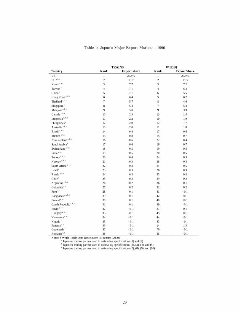
Table 1: Japan’s Major Export Markets - 1996

TRAINS WTDB† Country Rank Export share Rank Export Share US 1 26.4% 1 27.5% EU a, b, c 2 13.7 2 15.3 Korea a, b, c 3 7.7 3 7.2 Taiwan c 4 7.1 4 6.3 China c 5 7.1 6 5.5 Hong Kong a, b, c 6 6.4 5 6.2 Thailand a, b, c 7 5.7 8 4.6 Singapore c 8 5.4 7 5.3 Malaysia a, b, c 9 5.0 9 3.9 Canada a, b, c 10 2.5 13 1.4 Indonesia a, b, c 11 2.2 10 1.9 Philippines c 12 2.0 12 1.7 Australia a, b, c 13 2.0 11 1.8 Brazil a, b, c 14 0.8 17 0.6 Mexico a, b, c 15 0.8 15 0.7 New Zealand a, b, c 16 0.6 22 0.4 Saudi Arabia c 17 0.6 16 0.7 Switzerland a, b, c 18 0.5 19 0.5 India a, b, c 19 0.5 20 0.5 Turkey a, b, c 20 0.4 24 0.3 Norway a, b, c 21 0.3 28 0.3 South Africa a, b, c 22 0.3 21 0.5 Israel c 23 0.3 26 0.3 Russia a, b, c 24 0.3 23 0.3 Chile c 25 0.2 29 0.2 Argentina a, b, c 26 0.2 36 0.1 Colombia a, c 27 0.2 32 0.2 Peru a, c 28 0.1 41 <0.1 Bangladesh a, b, c 29 0.1 42 <0.1 Poland a, b, c 30 0.1 40 <0.1 Czech Republic a, b, c 31 0.1 39 <0.1 Egypt a, b, c 32 <0.1 37 0.1 Hungary a, b, c 33 <0.1 45 <0.1 Venezuela a, c 34 <0.1 44 <0.1 Nigeria c 35 <0.1 43 <0.1 Panama a, c 36 <0.1 14 1.3 Guatemala c 37 <0.1 76 <0.1 Romania a, c 38 <0.1 85 <0.1 Notes: † World Trade Data Base source is Feenstra (2000).

a Japanese trading partner used in estimating specifications (1) and (6) b Japanese trading partner used in estimating specifications (2), (3), (4), and (5) c Japanese trading partner used in estimating specifications (7), (8), (9), and (10)

29

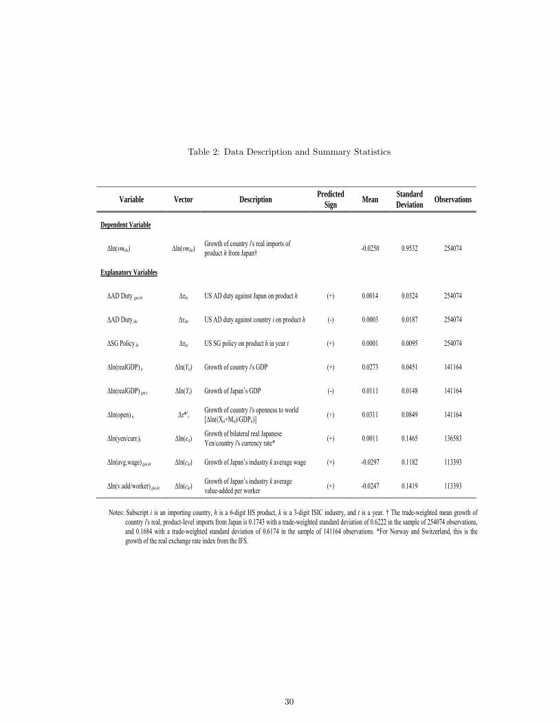
Table 2: Data Description and Summary Statistics

Variable Vector Description Predicted Sign Mean Standard

Deviation Observations

Dependent Variable

∆ln(vmiht) ∆ln(vmiht) Growth of country i's real imports of product h from Japan† -0.0250 0.9532 254074

Explanatory Variables

∆AD Duty jpn,ht ∆τht US AD duty against Japan on product h (+) 0.0014 0.0324 254074

∆AD Duty iht ∆τiht US AD duty against country i on product h (-) 0.0003 0.0187 254074

∆SG Policy ht ∆τht US SG policy on product h in year t (+) 0.0001 0.0095 254074

∆ln(realGDP) it ∆ln(Yit) Growth of country i's GDP (+) 0.0273 0.0451 141164

∆ln(realGDP) jpn,t ∆ln(Yt) Growth of Japan’s GDP (-) 0.0111 0.0148 141164

∆ln(open) it ∆τ*it

Growth of country i's openness to world [∆ln((Xit+Mit)/GDPit)]

(+) 0.0311 0.0849 141164

∆ln(yen/curri)t ∆ln(eit) Growth of bilateral real Japanese Yen/country i's currency rate* (+) 0.0011 0.1465 136583

∆ln(avg.wage) jpn,kt ∆ln(ckt) Growth of Japan’s industry k average wage (+) -0.0297 0.1182 113393

∆ln(v.add/worker) jpn,kt ∆ln(ckt) Growth of Japan’s industry k average value-added per worker (+) -0.0247 0.1419 113393

Notes: Subscript i is an importing country, h is a 6-digit HS product, k is a 3-digit ISIC industry, and t is a year. † The trade-weighted mean growth of

country i's real, product-level imports from Japan is 0.1743 with a trade-weighted standard deviation of 0.6222 in the sample of 254074 observations, and 0.1684 with a trade-weighted standard deviation of 0.6174 in the sample of 141164 observations. *For Norway and Switzerland, this is the growth of the real exchange rate index from the IFS.

30

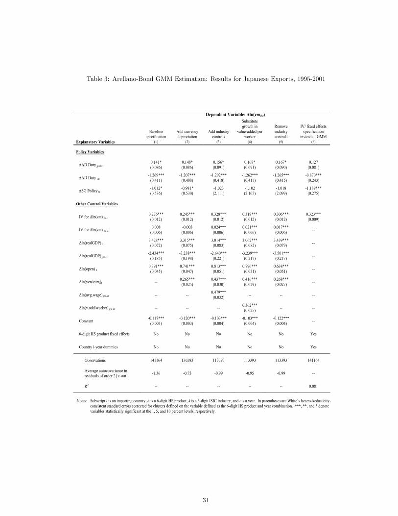
Table 3: Arellano-Bond GMM Estimation: Results for Japanese Exports, 1995-2001

Dependent Variable: Δln(vmiht)

Baseline specification

Add currency depreciation

Add industry controls

Substitute growth in

value-added per worker

Remove industry controls

IV/ fixed effects specification

instead of GMM Explanatory Variables (1) (2) (3) (4) (5) (6)

Policy Variables

ΔAD Duty jpn,ht0.141* (0.086)

0.148* (0.086)

0.156* (0.091)

0.168* (0.091)

0.167* (0.090)

0.127 (0.081)

ΔAD Duty iht-1.269***

(0.411) -1.207***

(0.408) -1.292***

(0.418) -1.262***

(0.417) -1.265***

(0.415) -0.870***

(0.243)

ΔSG Policy ht-1.012* (0.536)

-0.981* (0.530)

-1.023 (2.111)

-1.102 (2.105)

-1.018 (2.099)

-1.189*** (0.275)

Other Control Variables

IV for Δln(vm) iht-10.276*** (0.012)

0.245*** (0.012)

0.328*** (0.012)

0.319*** (0.012)

0.306*** (0.012)

0.323*** (0.009)

IV for Δln(vm) iht-20.008

(0.006) -0.003 (0.006)

0.024*** (0.006)

0.021*** (0.006)

0.017*** (0.006) --

Δln(realGDP) it3.428*** (0.072)

3.315*** (0.075)

3.014*** (0.083)

3.062*** (0.082)

3.439*** (0.079) --

Δln(realGDP) jpn,t-2.434***

(0.185) -3.238***

(0.198) -2.640***

(0.221) -3.239***

(0.217) -3.501***

(0.217) --

Δln(open) it0.391*** (0.045)

0.741*** (0.047)

0.813*** (0.051)

0.790*** (0.051)

0.638*** (0.051) --

Δln(yen/curri)t -- 0.265*** (0.025)

0.437*** (0.030)

0.416*** (0.029)

0.268*** (0.027) --

Δln(avg.wage) jpn,kt -- -- 0.479*** (0.032) -- -- --

Δln(v.add/worker) jpn,kt -- -- -- 0.362*** (0.025) -- --

Constant -0.117*** (0.003)

-0.120*** (0.003)

-0.103*** (0.004)

-0.103*** (0.004)

-0.122*** (0.004) --

6-digit HS product fixed effects No No No No No Yes

Country i-year dummies No No No No No Yes

Observations 141164 136583 113393 113393 113393 141164

Average autocovariance in residuals of order 2 [z-stat] -1.36 -0.73 -0.99 -0.95 -0.99 --

R2 -- -- -- -- -- 0.081

Notes: Subscript i is an importing country, h is a 6-digit HS product, k is a 3-digit ISIC industry, and t is a year. In parentheses are White’s heteroskedasticity-

consistent standard errors corrected for clusters defined on the variable defined as the 6-digit HS product and year combination. ***, **, and * denote variables statistically significant at the 1, 5, and 10 percent levels, respectively.

31

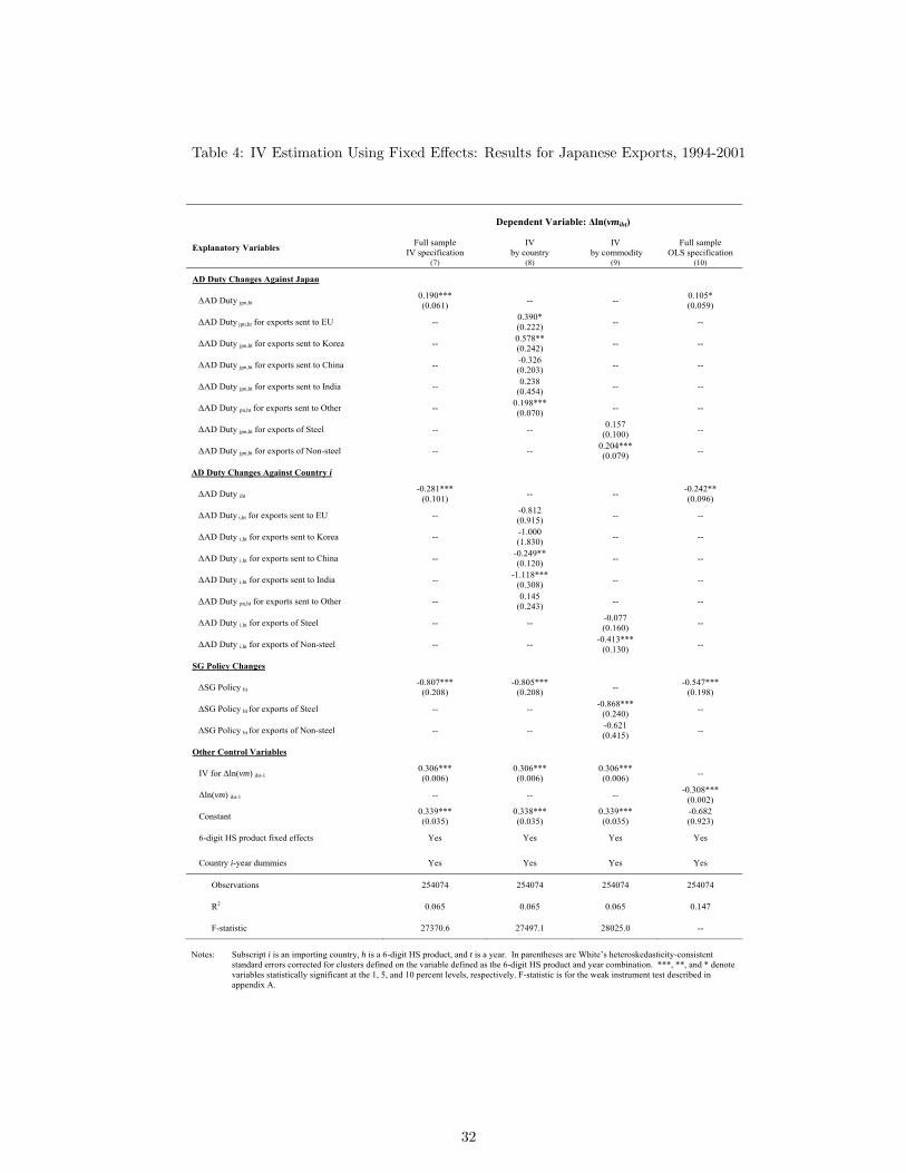
Table 4: IV Estimation Using Fixed Effects: Results for Japanese Exports, 1994-2001

Dependent Variable: ∆ln(vmiht)

Explanatory Variables Full sample IV specification

IV by country

IV by commodity

Full sample OLS specification

(7) (8) (9) (10)

AD Duty Changes Against Japan

∆AD Duty jpn,ht0.190*** (0.061) -- -- 0.105*

(0.059)

∆AD Duty jpn,ht for exports sent to EU -- 0.390* (0.222) -- --

∆AD Duty jpn,ht for exports sent to Korea -- 0.578** (0.242) -- --

∆AD Duty jpn,ht for exports sent to China -- -0.326 (0.203) -- --

∆AD Duty jpn,ht for exports sent to India -- 0.238 (0.454) -- --

∆AD Duty pn,ht for exports sent to Other -- 0.198*** (0.070) -- --

∆AD Duty jpn,ht for exports of Steel -- -- 0.157 (0.100) --

∆AD Duty jpn,ht for exports of Non-steel -- -- 0.204*** (0.079) --

AD Duty Changes Against Country i

∆AD Duty iht-0.281***

(0.101) -- -- -0.242** (0.096)

∆AD Duty i,ht for exports sent to EU -- -0.812 (0.915) -- --

∆AD Duty i,ht for exports sent to Korea -- -1.000 (1.830) -- --

∆AD Duty i,ht for exports sent to China -- -0.249** (0.120) -- --

∆AD Duty i,ht for exports sent to India -- -1.118*** (0.308) -- --

∆AD Duty pn,ht for exports sent to Other -- 0.145 (0.243) -- --

∆AD Duty i,ht for exports of Steel -- -- -0.077 (0.160) --

∆AD Duty i,ht for exports of Non-steel -- -- -0.413*** (0.130) --

SG Policy Changes

∆SG Policy ht-0.807***

(0.208) -0.805***

(0.208) -- -0.547*** (0.198)

∆SG Policy ht for exports of Steel -- -- -0.868*** (0.240) --

∆SG Policy ht for exports of Non-steel -- -- -0.621 (0.415) --

Other Control Variables

IV for ∆ln(vm) iht-10.306*** (0.006)

0.306*** (0.006)

0.306*** (0.006) --

∆ln(vm) iht-1 -- -- -- -0.308*** (0.002)

Constant 0.339*** (0.035)

0.338*** (0.035)

0.339*** (0.035)

-0.682 (0.923)

6-digit HS product fixed effects Yes Yes Yes Yes

Country i-year dummies Yes Yes Yes Yes

Observations 254074 254074 254074 254074

R2 0.065 0.065 0.065 0.147

F-statistic 27370.6 27497.1 28025.0 --

Notes: Subscript i is an importing country, h is a 6-digit HS product, and t is a year. In parentheses are White’s heteroskedasticity-consistent

standard errors corrected for clusters defined on the variable defined as the 6-digit HS product and year combination. ***, **, and * denote variables statistically significant at the 1, 5, and 10 percent levels, respectively. F-statistic is for the weak instrument test described in appendix A.

32

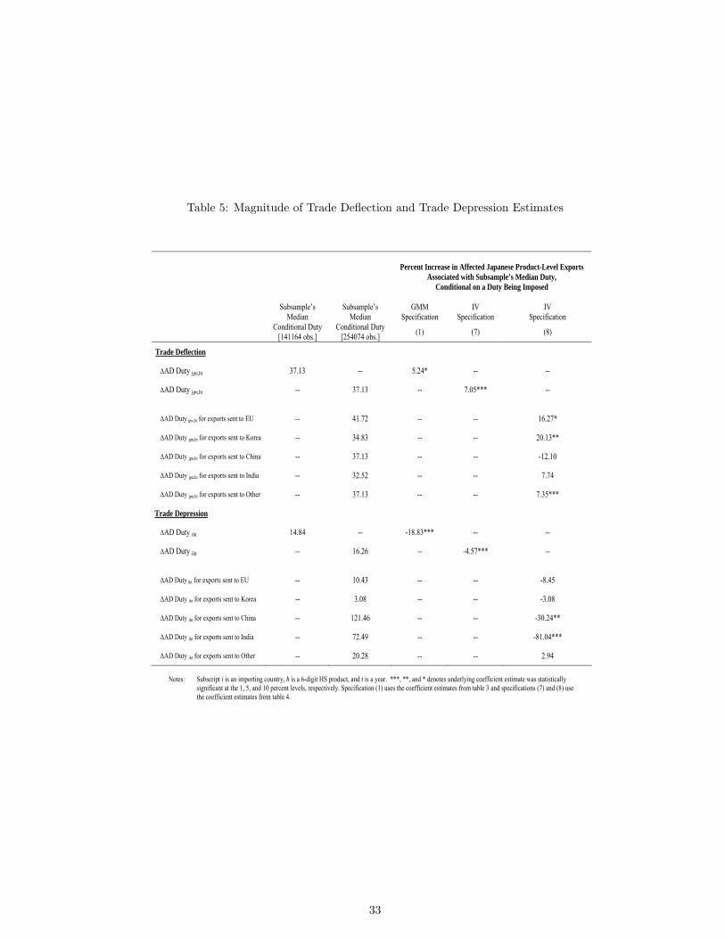
Table 5: Magnitude of Trade Deflection and Trade Depression Estimates

Percent Increase in Affected Japanese Product-Level Exports

Associated with Subsample’s Median Duty, Conditional on a Duty Being Imposed

GMM

Specification IV

Specification IV

Specification

Subsample’s Median

Conditional Duty [141164 obs.]

Subsample’s Median

Conditional Duty [254074 obs.] (1) (7) (8)

Trade Deflection

∆AD Duty jpn,ht 37.13 -- 5.24* -- --

∆AD Duty jpn,ht -- 37.13 -- 7.05*** -- ∆AD Duty jpn,ht for exports sent to EU -- 41.72 -- -- 16.27*

∆AD Duty jpn,ht for exports sent to Korea -- 34.83 -- -- 20.13**

∆AD Duty jpn,ht for exports sent to China -- 37.13 -- -- -12.10

∆AD Duty jpn,ht for exports sent to India -- 32.52 -- -- 7.74

∆AD Duty jpn,ht for exports sent to Other -- 37.13 -- -- 7.35***

Trade Depression

∆AD Duty iht 14.84 -- -18.83*** -- --

∆AD Duty iht -- 16.26 -- -4.57*** -- ∆AD Duty iht for exports sent to EU -- 10.43 -- -- -8.45

∆AD Duty iht for exports sent to Korea -- 3.08 -- -- -3.08

∆AD Duty iht for exports sent to China -- 121.46 -- -- -30.24**

∆AD Duty iht for exports sent to India -- 72.49 -- -- -81.04***

∆AD Duty iht for exports sent to Other -- 20.28 -- -- 2.94

Notes: Subscript i is an importing country, h is a 6-digit HS product, and t is a year. ***, **, and * denotes underlying coefficient estimate was statistically significant at the 1, 5, and 10 percent levels, respectively. Specification (1) uses the coefficient estimates from table 3 and specifications (7) and (8) use the coefficient estimates from table 4.

33

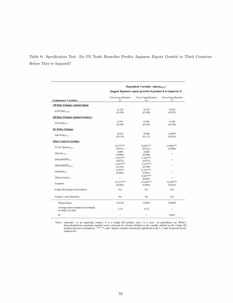
Table 6: Specification Test: Do US Trade Remedies Predict Japanese Export Growth to Third Countries

Before They’re Imposed?

Dependent Variable: Δln(vmiht-1)

[lagged Japanese export growth of product h to importer i]

Test of specification Test of specification Test of specification Explanatory Variables (1) (2) (7)

AD Duty Changes Against Japan

ΔAD Duty jpn,ht-0.124 (0.109)

-0.152 (0.108)

-0.053 (0.072)

AD Duty Changes Against Country i

ΔAD Duty iht0.391

(0.349) 0.396

(0.345) 0.148

(0.144)

SG Policy Changes

ΔSG Policy ht-0.016 (0.118)

-0.006 (0.117)

-0.099* (0.055)

Other Control Variables

IV for Δln(vm) iht-20.277*** (0.012)

0.245*** (0.012)

0.306*** (0.006)

Δln(vm) iht-30.009

(0.006) -0.002 (0.006) --

Δln(realGDP) it-13.425*** (0.072)

3.310*** (0.075) --

Δln(realGDP) jpn,t-1-2.412***

(0.185) -3.222***

(0.198) --

Δln(open) it-10.395** (0.045)

0.747*** (0.047) --

Δln(yen/curri)t-1 -- 0.267*** (0.045) --

Constant -0.117*** (0.003)

-0.120*** (0.003)

0.339*** (0.035)

6-digit HS product fixed effects No No Yes

Country i-year dummies No No Yes

Observations 141162 136581 254070

Average autocovariance in residuals of order 2 [z-stat] -1.35 -0.72 --

R2 -- -- 0.065

Notes: subscript i is an importing country, h is a 6-digit HS product, and t is a year. In parentheses are White’s

heteroskedasticity-consistent standard errors corrected for clusters defined on the variable defined as the 6-digit HS product and year combination. ***, **, and * denote variables statistically significant at the 1, 5, and 10 percent levels, respectively.

34

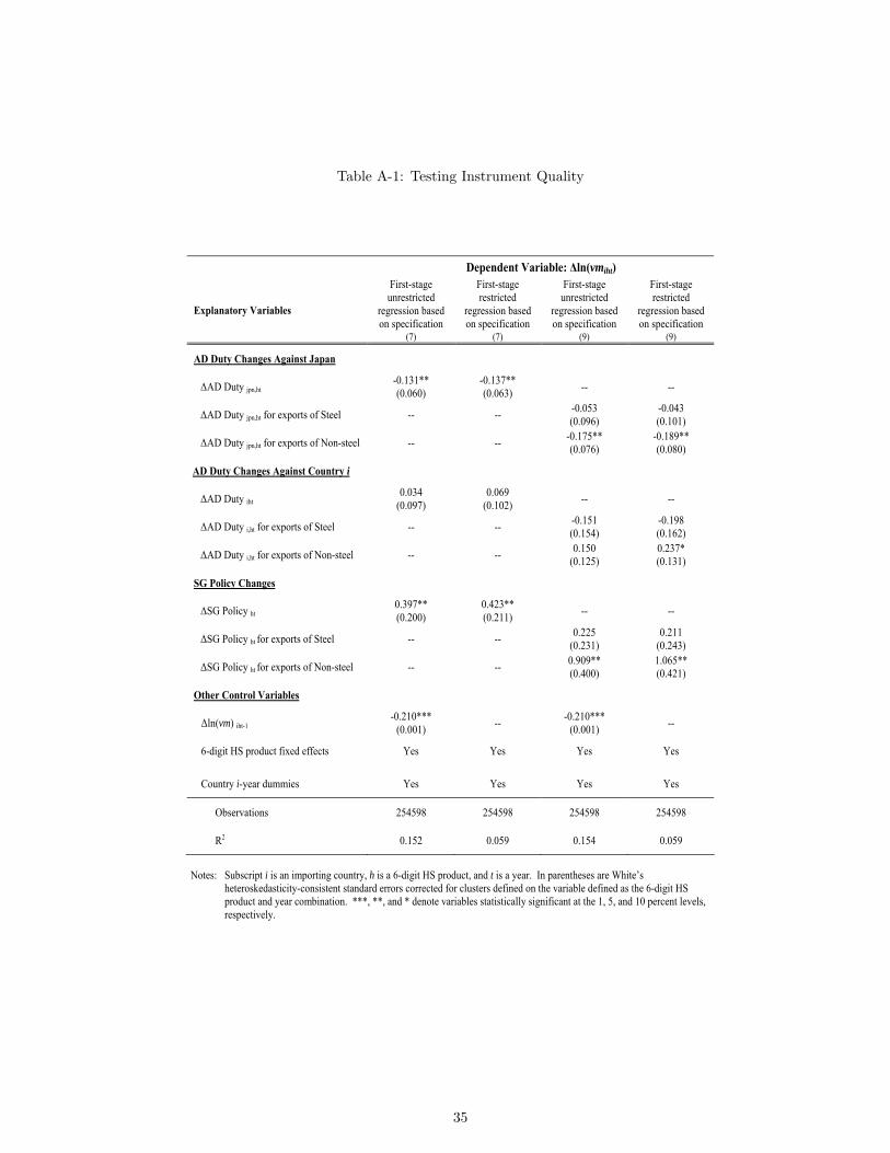
Table A-1: Testing Instrument Quality

Dependent Variable: Δln(vmiht) First-stage

unrestricted regression based on specification

First-stage restricted

regression based on specification

First-stage unrestricted

regression based on specification

First-stage restricted

regression based on specification

Explanatory Variables

(7) (7) (9) (9)

AD Duty Changes Against Japan

ΔAD Duty jpn,ht-0.131** (0.060)

-0.137** (0.063) -- --

ΔAD Duty jpn,ht for exports of Steel -- -- -0.053 (0.096)

-0.043 (0.101)

ΔAD Duty jpn,ht for exports of Non-steel -- -- -0.175** (0.076)

-0.189** (0.080)

AD Duty Changes Against Country i

ΔAD Duty iht0.034

(0.097) 0.069

(0.102) -- --

ΔAD Duty i,ht for exports of Steel -- -- -0.151 (0.154)

-0.198 (0.162)

ΔAD Duty i,ht for exports of Non-steel -- -- 0.150 (0.125)

0.237* (0.131)

SG Policy Changes

ΔSG Policy ht0.397** (0.200)

0.423** (0.211) -- --

ΔSG Policy ht for exports of Steel -- -- 0.225 (0.231)

0.211 (0.243)

ΔSG Policy ht for exports of Non-steel -- -- 0.909** (0.400)

1.065** (0.421)

Other Control Variables

Δln(vm) iht-1-0.210***

(0.001) -- -0.210*** (0.001) --

6-digit HS product fixed effects Yes Yes Yes Yes

Country i-year dummies Yes Yes Yes Yes

Observations 254598 254598 254598 254598

R2 0.152 0.059 0.154 0.059

Notes: Subscript i is an importing country, h is a 6-digit HS product, and t is a year. In parentheses are White’s

heteroskedasticity-consistent standard errors corrected for clusters defined on the variable defined as the 6-digit HS product and year combination. ***, **, and * denote variables statistically significant at the 1, 5, and 10 percent levels, respectively.

35