dynamically set lead times in mrp environments
TRANSCRIPT

University of Calgary
PRISM: University of Calgary's Digital Repository
Graduate Studies Legacy Theses
1997
Dynamically set lead times in MRP environments
Mattar, Roger
Mattar, R. (1997). Dynamically set lead times in MRP environments (Unpublished master's
thesis). University of Calgary, Calgary, AB. doi:10.11575/PRISM/24246
http://hdl.handle.net/1880/26731
master thesis
University of Calgary graduate students retain copyright ownership and moral rights for their
thesis. You may use this material in any way that is permitted by the Copyright Act or through
licensing that has been assigned to the document. For uses that are not allowable under
copyright legislation or licensing, you are required to seek permission.
Downloaded from PRISM: https://prism.ucalgary.ca

THE UNIVERSITY OF CALGAFiY
Dynamically Sec Lead Times
In MRP Environments
by
Roger Mattar
A THESIS
SUBKITTED TO THE FACULTY OF GE?A!XJATE STUDIES
IN PARTIAL FULFILMENT OF THE REQUIREMENTS FOR THE
DEGREY O F -WSTER OF SCIENCE
DEPARTMENT OF MECHANICAL ENGINEERING
CALGARY, ALBERTA
J U L Y , 1997
O Roger Mattar 1997

National Library 1+1 of,, Bibliothèque nationale du Canada
Acquisitions and Acquisitions et Bibliographic SeMces services bibliographiques
395 Wellington Street 395. rue Wellington OttawaON K1AON4 Ottawa ON K1A ON4 Canada Canada
The author has granted a ron- exclusive licence allowing the National Library of Canada to reproduce, loan, distribute or sell copies of this thesis in microform, paper or electronic formats.
The author retains ownership of the copyright in this thesis. Neither the thesis nor substantial extracts fiom it may be printed or otherwise reproduced without the author's permission.
L'auteur a accordé une licence non exclusive permettant à la Bibliothèque nationale du Canada de reproduire, prêter, distribuer ou vendre des copies de cette thèse sous la fome de microfiche/^ de reproduction sur papier ou sur format électronique.
L'auteur conserve la propriété du droit d'auteur qui protège cette thése. Ni la thèse ni des extraits substantiels de celle-ci ne doivent être imprimés ou autrement reproduits sans son autorisation.

Abs tract
Material Requirements Planning l o g i c is w i d e l y iised i n c h e
manufacture of discrete goods in batch productior?
env i romen t s . Y I P is of ton cri t icisec for pronocing excessive
work-in-progress inventory. This Fs related t o the use of
L s t a t i c planned l e a c times, which are s e to acccmmc~azs wcrs,
case scenarios,
in this research, it is proposeà t h a t lead cimes are set
ciynamically current s hop loads and batch sizes i n t o
acco~rit. The updated lead r i m e s a re used to set nore vziia
release and due dates f o r jobs.
A. literature r e v i e w is providea. An MRP syscern is i n t e r f a c e c
with the simulation of a production environment. The
p e r f c r m c n c e cf tne system r u n n i n g under s t a t i c lead tirne-: is
compared to the same when dynamic lead times are used. Resul t s
indicate t h a t when shop load fluctuates, dynamic lead t i m e s
can improve delivery performance. However, at very high loads,
the relarrionship used to set lead times is not responsive
enough.

Acknowledgements
Many t h a n k s go to
Dr. Van tnns, my supervisor, f o r h i s parrience, guiàance, che
many t o u r s , and for being a friend.
Dr. Gu a ~ d Dr. Balakrishnan of my examining comiCtee f o r
their effort in reviewing a n d examining t h i s thesis.
family; Tony, Samirâ a n d Johnny. Thanks f o r the food,
advice, s u p p o r t , encouragement and love.
extended family; Tante Hoda, Boss Zouzou, Louis, Shei la ,
Jarnil, Nada, Sarah , Jad, Car la , Pierre, Monique, and
A n d r e w .
The Departmerit of Mechanical Engineering, the University
Research Grants Cornittee and the Natural Sciences and
Engineering Research Council for their generous f i n a n c i a l
support of thls research.
Thank you also t o a l 1 those who helped me in many ways,
particularly Lynn Banach.

Table of Contents
Approval Page . . . .. . . . . . . . . . . . . . . . . . ii . . . - 1 ; - 4 b ~ t r â C t . . . . . . . . . . . . . r . . , . . . . . . --A
Acknowledgernents . . . . . . . . . . . . . . . - . . . iv Table of Contents . . , . . , , . , . . . . , . . . . . . v
L i s t o f A b b r e v i a t i o n s . . . . . . . . . . . . . . . - . . ix
1.0 I n t r o d u c t i o n 0 . . . . . . . . . . . . , 1.1 Introduction to MRP - . . . . . . .
1.1.1 Material Requirement Logic . 1.1.2 Time Phasing L o g i c . . . - . 1.1.3 MX2 Prerequisite Information
1.1.4 -!!P Assumptions . . . . . . . 1.1.5 MRP Applicability . .. . . .
1.2 The M W System . . . . . . . . . . . 1.2.1 Objectives , . , . . . . . . 1.2.2 Inputs and Outputs . . . . . 1.2.3 Record Processing . . . . . .
1.3 Alternatives to MRP . . . . . , . .
1.3.2 Drum-Bufler-Rope Scheduling .

2 .0 L i t e r a t u r e Review . . . . . . m . . . . . . . . . . 1 7
2.1FlowtimePrediction . . . . . . . . . O . . . 1 7
2 .2 Controlling L e a d Times . . . . . . . . . . . . . 22
2.3 Developments in MRP . . . . . . . O . . . . . 25
2 .4 Agile N a n c f a c t u r i n g Systems . . O . . . . . . 30
3.0 The Experimental Production Environment . 33
3.1 T h e Production F a c i l i t ÿ . . . . . . . . . . . . 3 3
3.2 Products fo rManufac tu re O . . . . . . . . . . 3 4
3 .3 Dernana Parsterns . . . . . . . . . . . . . . . . 35
3 . 4 Further Assumptions . . . . . . . . . . . . . 39 3.5 Modelling Che Productim Enviroment . 42
4.0SoftwareDevelopment . . . . . . . . . . . . . . O -
4 . 1 The Simulation Mode1 . . . . . . . . . . . . . . 4 . 1 . 1 I r i i i i a I i s z t i o n . . . . . . . . . . . . .
. . . . . . . . . . . . . . 4 . 1 . 2 O r d e r R e a d I n
4 . 1 . 3 Shop Floor Emulation . . . . . . . . . . 4.1.4 Data Collection . . . . . . . . . . . . . 4 . 1 . 5 The Experiment File . . . . . . . . . . .
4 . 2 T h e M R P S y s t e m . . . . o . . . . . . . . . . - .
4 . 2 . 1 Shop Floor Feedback . . . . . . . . . . . 4.2 .2 Updating L e a d T i m e s . . . . . . . - . . .
4 . 2 . 3 M R P Explosion . . . . . . . . . . . . . .


6.2.1 S t a t i s t i c a l Test R e s u l t s . . . . . . . . 94
6.2.2 Analysis . . . . . . . . . . . . . . . . 97
7 . 0 Conclus ions . . . . . . . . . . . . . . . . . . . . L03
7.lSummary . . . . . . . . . . . . . . . . 1 0 3
7 . 2 Future Work . . . . . . . . . . . . . . . 1C5 Bibliography . . . . . . . . . . . . . . . . . . . . . 107 Table cf Appendices . . . . . . . . . . . . . . . . . . 115
v i i i

L i s t of Abbreviations
BOM
CNC
CRP
CV
di
D E 2
EDD
ESOFT
FCS
ms
FT
GR
H.4
Hz
3IT
Exponential smoothing constant
Adapcive Forecast iriç Mcdel
Analysis of Variance
Bill of Materials
C o m p l e t i o n date of order i
Continuous Delivery Material Requirements 3 l a n n F n q
Confidence Interval
Cornputer N u m e r i c a l l y Controlled
Capacity Requir~ients Plann ing
C o e f f i c i e n t of V a r i a t i o n
Due date of order i
Drurn-Buffer-Rope scheduling technique
Ear l i e s t Due Date dispatching rule
Exponensially S m o o t h e d Operation Ç l o w t i m e
F i n i t e Capacity Scheduling
Flexible Manufacturinç System
Flowt ime
Gross Requirements
Alternate Hypothesis
Nul1 Hypothesis
Just-In-Time

MPS
MRP
OFT
OLT
rand
RCCP
TOC
TWK
TWKCP
VBA
WINS
WIP
Lateness of order i
Lot For Loc batch s i z i n g technique
L o t S i z e
Lead T h e
Master Production Schedule
Material Requirements P l a n n i n g
Mean
O p e r a t i o n F l o w t i m e
Operation Lead T i m e
. P e r c e n t Tardy
Random nurnber betweeri O and 1
Rough C u t Capacit y Planning
Standard deviation
Scheduled Receipts
M e a r i tardiness of order i
Theory of C o n s t r a i n t s
Tota l Work Con ten t
T o t a l Work Content on C r i t i c a l P a t h
Visüal Basic f o r - p l i c a t i o n s
Work i n Systems
Work-in-Progress inventory

Chapter One
INTRODUCTION
Materiai Requirements Plann ing (MRP) s y s r e m s a re u s e c i n t h e
manufac tu r e of discrete goods i n ba tch production
env i romer i t s . Developed in the 1960rs , MRP s y s t e m s are s t i i l
i n w i d e use today despite some well recognised weaknesses. The
i n t r o d u c t i o n of o t h e r production p l a n n i n g and control s y s t e m s
has not dampened e n t h u s i a s m f o r MRP: many companies look f o r
ways to adapt rhe NRP approach o r e n h a n c e t h e i r existing
systems (Vollrnann e t al., 1992).
1 t is g e n e r a l l y recognised thac p r o d u c t i o n environments
o p e r a t i n g unde r MRP c o n t r o l t end t o have high levels of work-
i n - p r o g r e s s (WIP) inventory a n d correspondingly long
manufacturing lead times. These n o t only worsen a cornpany's
f i n a n c i a l p o s i t i o n b u t make t h e shop f l o o r more congested and
d i f f i c u l t t o coordinate . It is claimed that this poor
performance is connec t ed to the way manufacturing planned lead
t i m e s are set. Oves the years, t h i s has led t o suggestions
t h a t lead times be set dynamically (e.g. Hoyt, 1978).
The o b 2 e c t i v e of t h i s research i s to test the hypothesis that

dynamically setting manufacturing planned lead times improves
t h e perfo-mance of MRP-controlled p r o d u c t i o n environments . Planned lead times f o r purchased prodwts continue to be
stacicaily sec. DynamFc lead times are expected to ad jüs t to
shop cond i t ions and main ta in the validity of t h e p l a n n e d lead
t i m e s .
T n e remairider of t h i r chapter is an introduction to MRP
systems. A rev iew of the l i t e r a t u r e is provided in chapter
two. The p r o d u c t i o n environment assumed i s defined i n c h a p ï e r
three and t h e f o u r t h chapter describes deve lopment of the
software. RI experirnental plan is discussed and outlined in
chapter f ive. I n chapter s i x t h e results are presented and
analysis of statistical tests i s underraken. Conclusions
drawn f r o m t h i s research are offered in chapter seven.
Some tems used extensiveiy throughout the thesis are defined
below:
L e a d time: the time allowed for an order to progress
through the shop floor (completion time - release time =
lead time). Lead time is planned, and is z l s o referred t o
as f l o w a l l o w a n c e or planned l e a d tirne-
Flowtime: the actrial tirne t h a t it takes for an order to
progress t h r o u g h t h e shop floor (frorn tirne of release

3
i n t o shop until tirne of completior?). Flowtime is not
planneci, and i s referred t o in some o f tne 1Fterotüre as
a c t u a l l e a d t i m e s -
Lecd 'Lime and f lowtiïne can be calccLazsd o r rneasured fcr
a single o p e r a t i o n - In such cases, we refer to the lead
cime p e r o p e r a t i o n and flowtime per O-erat ion.
1.1 Introduction to MRP
The aevelopment of MRP did n o t become possible u n t i l rrhe
advent of commercial cornputers i n the mid-1950's. As t h e power
o f computing became r e c o g n i s e d , existing inventory c o n t r o l
sys t ems (which were based on assumptions inappropriate for
manufacturing environments) Segan to be questioneà. IL? example
of assumptions used i n t h e s e systemç (e.g re-order point,
s t o c k replenishment) is the idea of inciependent demafid.
P roponen t s of MRP argued that demand for components used i n
production was not inciependent but depended on the demand for
t h e end item being produced. MRP was developed t o exactly
calculate the dependent dernand for components. Demand i s
defined as dependent when it derives from the demand for
another p r o d u c t . Dependent demand can be calculated and need
(should) n o t be forecast. Demand is defined a s independen t
when i t i s not d i r ec t l y related t o demand f o r any other items.

Independent
automobiles
independent.
plzyers for
4
demand has to be forecast. The demand for
from a manufacturer may be classified as
Demand by t h e manufacturer for stereo cassette
t h e same a u t o m b i l e s shoxlc! be c lass i f i eà as
dependent demand. The purchase of a stereo cassette player, by
a cuçtomer, from the manufacturer, as a replacement, however,
is classified as independent demand.
1.1.1 Material Requirement L o g i c
In actual production environments, there are many components
which are comon to several end items. It was recognised thac
demands for the same components by multiple parent parts or
assemblies shoula be j o i n t l y considered. Low-level coding was
developed in response to some of these concerns. Al1 bills of
materials are anzlyseci and tne lowest ievel in the product
trees a t which a component appears is identified. This low-
level code is added to cornponent recozds . When d e t e r r n i n i n g
gross requirements for al1 components, MRP processes al1
component records by level, highest first. The processing of
a record is therefore delayed until al1 requirements for the
component from higher ievels have been established (Orlicky,
1975) .

5
In many cases production or procurement of components involves
e-qensive setups o r long delivery tintes. To offse: t h e effecrr
of costly setups and long delivery times, different lo t sizing
r u l o s w e r e deve1ozed anci iised. L o t sizes w o i i l d Se sez to
arrive at a compromise between low costs and short batch
cimes. Such lot sizing techniques include economir order
quantiry, least t o t c l cost, ana l o C for lot. Full
explanations of these and other lot sizing rules can be found
in Meinyk and Piper ( 1 9 8 5 ) , Lunn and Neff (1982) ana Fogarïy
et al (1991) . Some additional principles of MEW systems are
outlined in the n e x t sections. These are t a k e n from OrlicKÿ
(1975).
1.1.2 Time Phasing L o g i c
The time intervals allowed to manufacture a component (or for
it to be delivered) are called planned lead tirnes. Lead times
are made up from estimâtes including queueing, setup,
processing and moving times. They are u s e d t o calculate
planned lead t i m e offsets for each component.
For example, an order for a desk is to be shipped at t h e end
of week 19, and the assembly lead tirne is one week. The
components for the desk (legs, desktop) must t h e n be ready by

6
the end o f w e e k 18. If it takes two weeks for delivery of t h e
legs, then the order must be.placed two weeks p r i o r to the end
of week 18 ( L e by the end of week 16). The desktop can be
manufactured in only one week. MRP will therefore release an
order authorising 2roducr ion to commence at the ena of week
17. An i m p o r t a n t feature here is t h e use of backward
scheduling . This, together w i ï h the time phasing, provides
coordination of parts going i n t o assembly. In the above
exampie, the legs are started a t a differenc t i m e t o the
desktop s u c h chat t hey bo th a r r ive a t Che same tirne for
assembly. This coordination reduces i n v e n t o r ÿ ( & n e n c e cos t s )
and improves work flow.
1.1.3 MRP Prerequisite Information
The following p o i n t s summarise the essential pre-requisites
for using MRP:
existence o f a mascer production schedule (MPS). The MPS
tells the MRP how much and when t o produce what e n d items
each i n v e n t o r y i t e m uniquely identified by part number
e x i s t e n c e o f a bill of materials ( B O M ) . T h e BOM
i d e n t i f i e s each manufactured item's components. BOM
structure o f t e n reflects p r o d u c t i o n procedure
availability of i n v e n t o r y records (may include part

number, batch s i z e , inventory s t a t u s , product
7
s u p p l i e r ,
lead time) for al1 items
availability of inventory
(e. g lot sizes)
i n t e g r i t y of ciata in z'iles
s ta tus anc! plznnlrig factors
Below are listed several important assuniptions for operating
MRP systems:
a planned lead times are specified for a i l inventory irems
every inventory i t e m goes i n t o
o n l y momentarily}
al1 components of an assembly
assembly order release
and out of stock (even
are needed at Che time
discrete disbursement and üsage of component materials
process independence of manufactured items. This means an
o r d e r for any i t e m may be started and f i n i s h e d and n o ï be
dependent on any other order for purposes of completion
The applicability of using an MRP system to generate component
release plans can be determined as follows:

8
end item requirernents are stated in the MPS. Gross
component requirements and t h e i r t i m i n g are derived by
the MRP from this MPS and the BOM's for the end items
discrete rnanuf actüring process
any level of product complexity
any discrete i t e m subject t o dependent dernand
1.2 The MRP System
This section looks at the objectives of MRP systems. Inputs
and o u t p u t s are listed. T h e MRP planning and control system
i s illustrateci.
The o b j e c ~ i v e of ali MRP systems is to dete-mine the
appropriate amount and timing of gross and n e t material
requiremects. T h i s information is used to generate correct
action pertaining to p u r c h a s i n g a n d production. Actions are
either new ones o r r e v i s i o n s of old ones. Revisions will
f r e q u e n t l y rnodify information on order quantity, release and
due dates.
Net requirements are always related to time and are covered by

9
planned or open orders. Planned orders are one of the ou tpu t s
of an LMRP system. They i n d i c a t ê a time in the f u t u r e when a n
o r d e r should S e placed wich a s u p p l i e r o r a work order
releasod t o t h e shop f loor . Planned orde r s become open o r d e r s
(also known as scheduled receipts) when t h e planner releases
the order t o the shop f l o o r o r t o a s u p p l i e r .
1.2 - 2 Inputs and ûutputs
There are f ive main i n p u t s into an MRP system:
master production schedule
inventory records
l o t sizing r u l e s
bills of materials
plamed l ead tirne d a t ~
Tho outputs of a n MRP system i n c l u d e :
cornponent order release and rescheduling
order cancellation notices
planned orders scheduled f o r r e l e a s e
i t e m status analysis b a c k u p data
inventory forecasts
notices
the f u t u r e
Figure 1.1 i l l u s t r a t e s i n more d e t a i l how MRP f u n c t i o n s wi thin

the overall frarnework of a production planning system. The
front end in figure 1.1 represents the longer te-m planning
portion. Resouce and product ion planning take a l o n g term
view. They dece-mine Company needs f o r the foreseeable f u i a r e .
Resource Production Planning Planning I
I 4
R C C P M P S Front End
C R P M R P
v Tirne-Phased
w Plans
Engine
F C S Order Release
w Vendor Shop Floor Control Control
Back End
Adapted from Vollmann, Berry, Whybark (7992) and Enns (1995a)
F i g u r e 1.1 MRP w i t h i n the production planning ana control hierarchy
The MPS can then be set f o r a n extended period using
guidelines set by market ing and production management. The MPS
is checked for feasibility using a rough cut capacity planning
(RCCP) tool. The engine portion represents the MRP system and

II
its associated inputs and outputs. The CRP module is described
in section 2.3. The routing file for a part descr ibes how t o
produce that part (which machine, tooling, setup times, etc).
Time-phased plans toke t he fom of orders, their release dates
and due dates. The back end in figure 1.1 dep ic t s the day-to-
day shop floor and vendor control system. A f i n i t e capacicy
scheduling (FCS) module may be run, using the plans generated
by MR?. FCS is discussed in secrion 2.3.
1.2.3 Record Processing
T h e basic MRP record is displayed i n table 1.1 This record
displays t h e following:
grcss requirements (GR): anticipatec fzture usage f o r the
item d u r i n g each time b u c k e t
scheduled receipts ( S R ) : existing replenishmenc orders
for the item due in at the beginning of each time bucket
projected on hand: current inventoxy ir! period i and
future inventory status for the item at the end of each
t h e bucket
planned order release: planned r e p l e n i s h e n t orders for
item at t h e beginning of each time b u c k e t
net requirements : Max (GR-SR-On Hand Inventory , 0 )

Table 1.1 The Basic YXP Record
A simple exarnple is shown in table 1.2 below. A product (P101)
i s assembled from several components, including two units of
component C102. A customer orders 120 units of Pl01 to be
delivered in period 3. The planned order for Pl01 is released
2 time buckets in advance (period 1). This is called lead time
offsettinç. The planned o r d e r s for the parent ( P101) become
the gross requirements for the component (C102). Records for
o t h e r cornponents that woulà be required fcr assembly of Pl01
would be filled in exactly the same way. Thus the components
ara coordinated tc arrive toge ther f o r assembly. for more
cornplicated product structures, the techniques used are
exactly the same. The d i f f i c u l t y lies in coordinating several
large end items with corrunon parts simultaneously.
In actual produc t ion environments, most end items involve
several assembly stages. Part numbers will change several
times, as different stages of assembly are reached. At each of

these stages, a work order may be required to allow a part to
continue through the shop.
LT=
2
LS=
1
Table 1.2 A Simple Example of MRP Records
LT=
I
tS=
40
In t h i s research, the product s t r u c t u r e s used are simple
enough and involve no commonality of parts. They are described
f u r t h e r ir;, chapter tnree. Therefore once an order is released
to the shop floor, assembly is assumed to be authorised at the
time al1 components become available. Although MRP systems do
not work in this way in real life, this method will not have
a s i g n i f icant impact u n t il product complexity increases
substant i a l l y .
Part: Pl01 Gross Requirements
Scheduled Receipts
Pro jected On Hand
Net Requirements
Planned Order Releases
P a r t : Cl02 Grass Requirements
Scheduled Receipcs
Pro jectea Or? Hznd
Net Requirements
Planned Ozder ReLeases
50
P D
225
25
2 s
110
1 220
40
45
15
10
2
45
120
P D 1 2 3 4 5 6 7 8
O
120
O
110
7 O
3 1 4 O
25
95
7 0
O
70
1s
25
4c
O
1 5
O
15
4 . 5 3 O
35
2s
O
35
6 7
35
8
35

1.3 Alternatives to MRP
Produc t ion p l a n n i n g and c o n t r o l systems can be diviaed into
t h r e e broad classes: 'pushr systems, which i n c l u d e M W , ' p u l l r
systems like just-in-time (JIT), and t h o s e based or? t h e theory
of c o n s t r a i n t s (TOC) , such as drum-buffer- rope ( D B R j
s c h e d u l i n g . I t c o u l d be argued t h a t DBR is a hybrid \ p u s h r -
r p u l l ' system. Browne e t a l . (1996) offer a good comparison o f
t h e s e t h r e e systems.
P u l l sy s t ems maintain a constant level of WIP on t h e shop
f l oo r . An order cannot be released u n t i l a n o t h e r h a s finished.
Push systems release o r d o r s as n e c e s s a r y i n order t o have then
completed by t h e i r due date. The level of WIP f l u c t u a t e s .
1.3.1 Ri11 Systems
The Kanban p r o d u c t i o n control system has received s i g ~ i f i c a n t
a t t e n t i o n r e c e n t l y . A great deal o f benefit has been ga ined i n
many p roduc t ion environments from t h e emergence of J I T sys tems
us ing Kanban p r o d u c t i o n c o n t r o l . T h e irnprovements that needed
t o be implemented t o make Kanban f e a s i b l e , such as s e t u p tirne,
batch s i z e and process variability r e d u c t i o n , can be
b e n e f i c i a l t o any Company. Due t o t h e v e r y small b u f f e r s i z e

between s t a t i o n s , however, Kanban r e q u i r e s a very stable
p r o a u c t i o n environment, where demmd can be smoothed out. For
example, Toyota Motor Co-rporationrs p roduc t ion plan covers one
yoar a n d is updaced monthly (Vol lmâr rn et al., 1992). In rnariy
environments, demand patterns cannot be smoothed out this well
meaninq that O u f f e r sizes must be much h i g h e r . In c h i s
respect, MRP systems have proven to be more u n i v e r s a l l y
applicable thari J I T systems, since t h e y cape better witn
variability.
1.3.2 D m - B u f f e r - R o p e Scheduling
Drurn-5üffer-rope (DBR) is a schedu l ing t o o l based on TOC ideas
d e v e l o p e d by Goldrat t ( G o l d r a t t and Cox, 1 9 9 2 ) . DBR assumes
t h e existence of a b o t t l e n e c k resource and acknowledges that
the throughput of t h e f a c i l i t y will be dictated by t h a t o f t h e
bottleneck. DBR then advocaïes placing p r i o r i t y on keeping t h e
bottlenecks busy. Work is fed i n t o t h e sys t em a t a r a t e
consistent w i t h t h e bottleneck r e s o u r c e r s t h r o u g h p u t . The
ob j ective is to keep the bot tleneck r e s o u r c e busy while
m i n i r n i s i n g i n v e n t o r y flowing to the b o t t l e n e c k . Tt c o u l d be
argued t h a t w i t h DBR, work is pulled through to the
bottleneck, and pushed downstream from t h e b o t t l e n e c k .

16
DBR, l i k e J f T , forces people to examine what is really going
on and find ways to improve the situation. Both JIT and DBR
stress continuous improvement. A big b e n e f i t of TOC is t h a t i c
h a s challenged t h e t r a d i t i o n a l thinking which e n c o u r a g e s non-
b o t t l e n e c k r e s o u r c e s t o keep producing unwanted parts j u s t to
maintain high efficiencies. Instead, it p u t s forward the
c o n c e p t tna t l o t sizes at non-bottleneck r e s o u r c e s may be
l o w e r e d ( e v e n with additional setups t h a t will be incurred)
since tnere is capacity l e f t over (Enns, 1995a ) . This dynamic
variation of lot sizes leads to lower inventories and
flowtimes.
It is anticipated that dynamically setting lead times in MRP
would have the same effect as DBR, since lead times at the
b o t t l e n e c k resource w i l l i n s r i n c t i v e l y D e h i g h e r t o ref lect
t h e longer queues. Perhaps it is time that MRP systems are
developed to take accoun t of these ideas and move forward into
the 2 1 s t century.

Chapter Two
LITERATURE REVIEW
T h i s chapter presents a review of topical literature. It is
divided into f o u r sec t ions . Literature on flowtime prediction
is presented in the first section. This is followed by a
review of load-orienired rnanufac tur ing control. Seccion three
looks at t h e development of MRP systems. The final section
considers agile rnanufacturing systems.
2.1 Flowtime Prediction
F l o w t i m e prediction per t a ins to t h e ability to a c c u r a ~ e l y
forecast how long an order w i l l take to progress th rough a
workstation or cne e n t i r e shop f l o o r . Flowtime prediction is
important as it would allow planned lead times to be adjusted
in order to maintain their validity. The = s e o f valid lead
t i m e s allows the MRP to compute valid release and due dates.
Most cf t h e l i t e r â t u r e on flowtime prediction and düe àate
setting concentrates on job shop enviroments (Conway et a l . ,
1 9 6 7 ) . After this literature is reviewed, some research which
considers assembly is examined.

18
Flowtime estimates can be static or dynamic. Static estimates
may be found from cpeueing analysis or steady-state simulation
results and are constant over Cime. Dynamic estimates may be
obtained using various inputs as predictors. For example,
regressior i equations wnick incorporate shop scatus and job
information may be developed. They can be derived to predict
accuai lead rimes (flowtimes) using hisccrical àata, and m à y
include terms like total work in shop and order 3atch size. As
Their values fluctuate, the predicted ac tua l lead time will
change too. The estimates of actual lead times from these
rnoàels rnay be used to set planned lead times.
One f o m of static flowtime prediction is queueing analysis.
Very b r i e f l y , a system is treated as a network of queues.
Using established relationships and utilisation levels, queue
l e n g t h s and flowtimes rnay be detemined. Planned Lead times
are calculated based on steady-state flowtime estimates and
used in due date setting. A more cornpiete account of t h i s
process is g i v e n in Enns (1993). Several tools are now
commercially available whicn use queueing heuristics including
Queu ing Network Analyser (Whitt, 1983) and MPX (Network
Dynamics, 1991 and Suri and de Treville, 1991)
Baker (1984) surveys sequencing and due date assignment rules

19
in job shops. While none o f the due date assignment rules
considers shop s t a t u s , he concludes t h a t Que dates s h o u l d
r e f l e c t work c o n t e n t . Recenï ly due date setting rias stârted CO
consider dynamic shop status. Bertrand (1983) uses tinte-phased
w o r k l o a d information ana time-phased capacity information t o
set due dates. Jobs are r e s c h e d u l e d for l a te r p e r i o d s when
c a p a c i t y i s u n a v a i l a b l e . A r e d u c t i o n i n l a t e n e s s v a r i a n c e i s
reported. A survey of due date assignment r u l e s by Ragatz and
Mabert ( 1 9 8 4 ) concludes t ha t r u l e s which c o n s i d e r shop status
and job i n f o r m a t i o n (e.g Jobs I n Queue) perform better t h a n
those which o n l y c o n s i d e r job i n f o r m a t i o n . Vig and Dooley
(199 l )p ropose a mixed estimate by combining s t a t i c and dynamic
e s t i m a t e s i n a l i n e a r weighted form. The aim is t o cornbine t h e
accuracy (no Mas) of s t a t i c estimates wi th the precision (low
variance) of dynamic estimates. T h e rnethod reduced but did not
eliminate bias. Chang (1996) develops a h e u r i s t i c f o r dynamic
job shop schedu l ing which estimates queue times and feeds them
b a c k t o the scheduler for improved performance. The most
signif i c a n t factor is idemif ied f rom samples u s i n g analysis
of var iance (ANOVA, see Devor et al., 1992) . T h i s is f o l l o w e d
by c o n s t r u c t i o n of a rule based on t h i s factor. His results
show t h a t t h e use of queue time estimates improve due date
per formance (mean tardiness and p e r c e n t tardy). Cheng and
Gupta (1989) s u r v e y due date a s s ignmen t r u l e s f o r job shops.

20
The literature reviewed which examined the use of shop status
information supports the conclusion that making use of shop
status information uhen setting due darrês h e l p s improve due
date performance. Lawrence (1995) models flowtime prediction
as s forecasting problem. The actual flowtirne is made up of c
flowtime estimate plus a n error tem. The error term is a
random variable estimated using a method of moments. Job lead
times and due dates are t h e n calculated. The method works well
in single semer networks but performance deterioratos i11 more
complex environments .
Goodwin and Goodwin (l982), study che relative impact of
different operating policies on the performance of an assembly
shop. They snow Chat not a l 1 job shop r e s e a r c h can be
generalised to assembly systems. Fry et al. (1989) test
several due dace setting rules in an assen ib ly environment.
Nine different product structures (3 tall, 3 f l a t , 3 mixed)
are a n a l y s e d in a simulation using che earliest due date (EDD)
sequencing r u l e . The due date setting r u l e s include total work
content ( T W K ) , total work content on the critical path
(TWKCP), work in system (WINS), a n d combinations of these
three. As with the l i t e r a t u r e on job shops, they conclude that
rules that consider shop status information (combination of
TWK or TWKCP with WINÇ) work best. Enns (199513) presents a

21
forecasting approach to flowtime prediction. The adaptive
forecast ing nodel (AFM) developed considers snop loading,
workload conditions and job characteristics i n setting due
dates. The nodel i d j u s t s to changes, since data on due date
performance is dynamically fed back t o it. The model perfoms
well under u n b a l a n c e d shop loads. T h i s mode1 is t h e n adapted
by Enns (1 995c) for assembly environments . Flowtime f orecasts are deteminoci for various production stages a n d are stackeà
according. to product structure. As in MRP, release dates for
components a re obcained by backward s c h e d u l i n g from ïhe end
iten due date. Lead times for operations are updated. Unlike
MRP, this model does n o t g e n e r a t e assembly order releases, and
- iïet r equ i r e rnen t s are assumed to equal gross requirements. in
other words, since al1 order releases are assumed to be
dedicated to a specific end item requirement, lot-for-lot
batch sizing is used and assembly is assumed to be autnorised
at the cin.e al1 cornponents are available. The mode1 perfoms
well under assembly conditions.
The next step in t h i s evolutionary process is to l i n k an
actual MRP system to a shop f loor emulated by a simulation
model. If lead times are a d j u s t e d to reflect actual shop
conditions, a dynamic MRP system which can respond to changes
in the production environment should result.

2.2 Con-olling Actual L e a d Times (Flowtimes)
As with the literactlre on flowtime prediction in section 2.1,
most of the literature on c o n t r o l of lead times also focuses
on jo5 shops. Ir is generally acknowledged t h a t queueing t h e s
frequently make up 90% or more of actual lead times for a
product. Hence it is important t o control leac! cimes for
several reasons. F i r s t l y , the time spent queueing is not
productive beyond what is required to bilffer againsr
uncertainty and variability. Secondly, long queues lead to
congestea shop f l o o r s which are d i f f i c u l t t o manage.
Wight ( 1 9 7 0 ) identifies errat ic order input and l a c k of
control over outpu t rates, togecher w i t h lead t i m e i n f l a t i o n
as the reasons why many p l a n t s have very l o n g backlogs ( i n
some cases 1 year o r more) when two weeks woulc! n o m a l l y
suffice. Such backlogs have t h e i r o r i g i n s i n capacity
botclenecks and excessive work input. Wight proposes
input/output control to remedy the s i t u a t i o n . His ideas are
based on t h e axiom that shop floor input must not exceed shop
floor output capabilities. He also places responsibility for
s e t t i n g order priorities and order release squarely with the
production control department and not the shop foreman.
E r r a t i c customer demand is smoothed out t o m a i n t a i n planned

rates of input. Onur and Fabrycky (1987) develop and test a n
input/output control system for a job shop. I n p u t and output
are controlled f o r t h e whole shop,
centres . Job release and capacity are
shop d u e date perfcrmance.
not individual work
con t rolled to improve
Spearman ec a l . (1990b) divide lead time reducticn stratecies
i n t o f ive c a t e g o r i e s : elimination of variability; work f low
smoothing (includes l e v e l l i n g of work loads); synchronisation
of produc t ion (becween fabrication and assembly, f o r
i n s t a n c e ) ; keep t h i n g s moving (smaller batches at non-
bottleneck w o r k c e n t r e s ) ; ar,d elimination of unnecessary WIP.
They r e c o g n i s e the value of WIP a t bottlenecks and observe
thai reduction o f mean flowtime and flowtime variance reduces
lead times. Speaman et al. (1990a) also propose a new control
system called CONWIP (CONstant WIP) for use in flow l i n e s . Ft
allows WIP t o collect i n f r o n t of b o t t l e n e c k s . They clairn
reduced levels of W I P when compared t o JIT systems.
Bechte (1988) and Wiendahl (1995) propose a c o n t r o l system
t h a t iç s imi lar but more detailed than CONWIP. It i s ca l led
load-oriented manufacturing control. Feedback from a job s h o p
i s evaluated. Actual lead times are compared to planned lead
times. Order release is controlled to keep WIP inventory at a

24
controlled level. This maintains actual lead times at a
planned and predetermined level. Orders may be domloaded from
an MRP systern. In such cases, the lead times used i n t h e MRP
cari be set equal t o t h e planned and pre-determinea l n v e l
mentioned above. S i n c e shop load is controlled the validity of
those s t a t i c lead times is betcer rnaintained.
Watson et al. (1993) use b a c k w a r d simulation t o generate
component release plans. Starting with due dates, jobs pass
through a simulation model of the snop Dackwards ( L e .
assembly operations become dis-assembly operat ions) . The
finisn t i m e in bzckward simulation is rhen recordec 2s the
release date for the component. A forward simulation run is
then done to check feasibility. These component plans (which
would n o m a l l y be generated by an MRP system) are t h e n
downloaded to a shop floor control system, in this case a
s imula t ion-based scheduler. T h e rnodels for generating these
pians are deterministic, much like those used in FCS. Only one
replication needs to be made so the simulation is very fast.
However, stochastic environment characteristics such as
process inç tirne variability, machine breakdown, and future job
arrivals are not represented. Deterministic models are less
realistic than stochastic models s ince schedules quickly
becorne invalid as uncertainty is introduced.

25
Hoyt (1978, 1982) puts the blame for poor MRP performance on
the improper setting of lead times, n o m a l l y s e t t o cover al1
scenarios. Planned lead times are supposed to indicate the
time for a job to go through the shop floor. If they are
wrong, che release a n a due daces calcuiated w i l l a l s o be
wrong. This leads to a host of problems (Hoyt, 1982). Aoyt
advocates setring the lead times dynamically for each work
station using equation 2.1. Exponential smoothing of the two
terms in the equation is süggested to reduce MRP nervousness
and dampen
Actua2
fluctuations. The lead time file is then updated.
Avera ge L T = Average Queue for Peri od Average Ou tpu t f o r same P e r i od
- (2 -1)
Such a calcula t ion of lead time considers queue times, shop
status, t r ans fe r times, s e tups , and almost a n y other f ac to r .
Despite its veaknesses, MRP has developed irito perhaps the
dominant production planning system in North America today.
Some of MRPrs strengths include the ability to handle large
volumes of data and many changes. Whybark and Williams (1976)
identify four sources of uncertainty (combinations of demand
o r supply, and t i m i n g or quantities). They propose a safety

26
lead time concept t o cover for uncertainty in timing and
safety stocks to cover uncertainty in quanticies. MRP systems
are insensitive t o capacity, that is , they assume that w h a t
car! 5e scheduled can be made. It is assumed thac capscity
considerations are t a k e n care of in the formulation of the
MPÇ. The earliest attempts Co consider capacity were the rough
cut capacity planning (RCCP) methods. They were designed t o
e n s u r e MPS feasiSilicy before the MRP generated its plans.
This was to avoid unnecessary MRP runs, s i n c e computer time
was expensive. These methods were only approxirnace. The next
developrnent was the closed-loop MRP which included a capacity
requirement planning (CRP] module. Oden et al. (1993) o f f e r s
an excellent review of CRP. The closed-loop is highlighted by
t h e bold arrows i n figure 1.1. The CRP module checks the plans
generated by the MRP for feasibility. If in feas ib le ,
adjustments should made ir! the MPS and/or to capacity be= ore
the MRP I s ruri again. If feasible, the time-phased MRP plans
are released to the shop f l oo r . Enns (1995a) identifies
several problems with CRP. While a p lan may be feasible in
CRP, t h a t is no guarantee the work can be compieted within a
specified time bucket. Work is placed in buckets specified by
stacking lead time allowances d u r i n g backward scheduling. If
the lead times are invalid, work gets placed i n the wrong
buckets. There is a l s o another problem related t o lead time

27
setting. As shop loads i n c r e a s e , average operation waiting
times are also expected to. increase due CO longer queues.
Since t h e iead times used by CRP remain unchanged, it does n o t
a n c i c i p a t e changes i n expecred w a i t i n g cimes. T h e loading
p r o f i l e s generated by CRP become less realistic. CRP w i l l not
f i x problems r e l a t i n g t o capacity; it is up CO che planners to
manually fix t h e problem. CRP uses i n f i n i t e loading
assumpt ions , like MRP, s o capacity is v i r t u a l l y ignoreà when
the load report is produced. Capacity violations must be
manually identified by the planners and fixed. Lasrly, CRP i s
n o t a scheduling t o o l , s i n c e it does not determine specific
s t a r t cimes for opera t ions o r oven the sequence in which to
process jobs competing fo r the same machine.
The most recent development has been finite capacity
scheduling (FCS) systems. Wyman (1993), Roder (1993) and Enns
(1995e, 19965) describe FCS in greater d e t a i l . When FCS
systems are run u n d e r M W , detailed schedules f o r a l 1
opera t ions are generated based on MRP release and due date
outputs. These schedules can be displayed as Gantt charts.
Detailed s c h e d u l e s also p r o v i d e forward v i s i b i l i t y , so
problems are identif ied earlier. Several problems are s t i l l
outstanding though. Any changes in shop c o n d i t i o n s will r e n d e r
t h e schedule invalid. If the frequency of changes is high ,

28
forward visibility decreases precisely when it is required
rnost- The other problern is t h a t of lead times. If the lead
times used by t h e MRP to calculate release and due daces ore
invalid, then zhe schedule generaced by cne C E is also
invalid. Static lead times, designed to cover al1 scenarios,
are almost always invalid. Establishing a feedback ioop to the
MRP would allow lead times to be adjusted based on c u r r e n t
w o r k load conditions. The focus of t h i s research is to t r y and
l Resou rce Production Planning Planning I R C C P k-f M P S Front End
1Y
M R P
1 6 1 y Lead Time
I Pians 1
/ I Engine /
r F C S > Order
Release Back End . . ,
Vendor Shop Floor Fee-k Control Control
Adapted from Vollrnann. Berry. Whybark (1992) and Enns (1995a)
Figure 2.1 Production planning and con t ro l w i t h feedback on shop status to t h e MRP

29
establish t h i s feedback. Figure 2 .1 illustrates one way the
MRP system could look with such a feedback loop.
There have been many other developments. Many relate tu the
development of add-on modules to support other functional
areas like f inance , account ing, hurnan resources and marketing.
This has led to tne acrcnym MRPII (manufacturing resources
planning) to distinguish it from the basic MRP. Fogarty et al.
(1991) o f f e r a good description of MRPII. However, there are
still some fundamental issues which seem to have been
overlooked i r ? the drive for a bettes MRP system. With very f e w
excep t ions the basic logic behind MRP has remained unchanged
for over thirty years. One such exception is put fo-mard by
Piper and Kuik (1988). They suggest a continuous delivery MRP
(CDMSP) s y s t e m . Unlike conventional M W systems where al1
input materials must be delivered p r io r to the start of a
p l a n n e d o rde r , CDMRP a l lows components t o be delivered in
small transportation batches to the point of use. Whereas i n
conventional MR? the lead times are stacked a c c o r d i n g to
product structure, lead times in CDMRP can overlap, with an
overall reduction in both WIP inventory and product lead
times. CDMRP works best when variability is rninimised and
setups are s h o r t , much l i k e in J I T environments. CDMRP s e e k s
to make production flow continuously.

2 .4 Agile Manufacturing Systems
This seccion presents s general look ae worlu manufacturi~g
trends. From a technological point of view, there has been a
trend towards automation in discrete par: manufacturing. This
trend started with Henry Ford in 1909 and has been accelerated
by the advent of the cornputer in rrhe 19501s. Robots were
introduced in the 1960's and by the 19701s, cornputer numerical
contro1 (CNC) was a reality. In the 1980's flexible
manufacturing systems (FMS) were becoming commonplace. From
the production management point of view, there have been cwo
worla streams. In the 1950's and 196O1s, throughput was the
most important consideration for Western companies. This was
a u e to the high levels of consumer demand following the en& of
the second world war. At the same time, Japanese firms were
focusing on producr: quality in an artempt to gain a
competitive edge and enter world markets. By the early 19801s,
Japan had becorne an economic and manuFacturing superpower.
While Japanese and Western corporations boasted similar
advanced manufacturing rechnology, Western companies were
still engrossed in mass production while their Japanese
counterparts were practising l e a n manufacturing. This was
exemplified in the development and use of the JIT
manufacturing philosophy . As market sharê was continuously

31
being lost to the Japanese, a radical shakeup of Western
thinking was required. Concurrent ençineering was the next
paradigm to take hold. Bedworth et al. (1991) offer a n
explanarion of what concurrent engineering is a l 1 about.
Briefly,
pro j ect
earlier,
overcome
inter-departmental personnel work together on a
and identify potential problems in design much
when it would be easier, faster and cheaper to
such problems.
The current trend (and one that is not likely to change) is
towards s h o r t e r product l i f e cycles, more customisation, lower
volumes, and rapid customer demand. The rnanufacturing
enterprise of the past or the present is not going to be
enough for many cornpanies to survive. What is (will bel needea
is an ability to make use of people's talents and respond
quickly to changing conditions. Innovation will have to corne
from al1 parts of the Company, not j u s t the R & D department.
Agile manufacturing (Kidd, 1994) is the t e m used to describe
such abilities. Concurrent engineering, lean rnanufacturing or
flexible manufacturing alone do not constitute agile
manufacturing, yet these and other techniques, tools and
methodologies must be present fo r a manufactur ing entity t o be
agile. Agile manufacturing is not a tool, but a concept. It
implies radical changes in the way manufacturing systerns, and

even whole organisations, are designed. Knowledge will become
ever more important, and harnessing the knowledge of people in
the e n t i r e organisation will be vital for survival.
Motivation for che development of MRP sysrems in the 1 9 5 0 ' s
was lower inventory levels coupled with better delivery
performance. The motivation today for dynamically setting lead
times is still the same, that is to lower inventory levels and
improve delivery performance. New information technology
together with new ideas and approaches make this a
possibility. This is consistent with the aims and ideas of
agile manufacturing.

Chapter Three
THE EXPERIMENTAL PRODUCTION ENVIRONMENT
The ob jec t ive of this chapter is to describe and j u s t i f y the
production environment assumed in the research. The f i rs t
section describes the produc t ion facility, including t h e
layout. The second s e c t i o n considers the products to be
na~ufactured in t h e facilitjr. Section three lcoks at t h e
demand pa t t e rns for the products. Assumptions are stated i n
section four, anc in s e c t i o n f i v e a modei of t h e production
environment b u i l t using rapid rnodelling s o f t w a r e is described.
3.1 The Production Facility
The p r o d u c t i o n facility assumed is the same as that proposed
Dy Enns (1996). There are f o u pre-assembly stations, one
assembly station and two post-assembly s t a t i o n s . Each o f t h e
seven stations has one machine whic:? is capable of performing
a single type of operation. No task preemption is allowed,
hence once a job is started, it must be finished before that
machine becomes available to another job. There is no scrap
and machines do not breakdown or require maintenance. The
facility works one eight-hour shift per day, seven days a

week. There is no overtime allowed. Queue l eng ths and work-in-
progress (WIP) levels are n o t restricred. Transportat ion t b e s
between machines and stations are assurned t o be zero- For
every p r o d ~ c c at each operation, there is a fixed setup tirne
fol lowed by a processing time which is dependent on t h e batch
size. There iç variability in t h e processing time b u t n o t in
the s e t u p time. Figure 3.1 i l l u s t r a t e s t h e assumed layout of
the facility.
C
' , Press Packing ' 3 c + Saw - Station -i' -0 cn - Co
2.1 - ,"'. ';\ VI- L w m . , ' BR*e \\ ES - O CI
Weiding 3 Shear -> Punch Station Paint . - Booth
~-> Material Flow F i g u r e 3.1 Layout of assurned product ion f a c i l i t y
wi th p o s s i b l e material f l o w routes
3.2 Products for Manufactu~e
Two sets of products are identified for manufacture. Each set
is made up of t w o f i n i s h e d products , n a e d Pl and P2. There is
no commonality of parts, hence t h e components tha t go i n t o
making Pl are not required for producing P2, and v i c e versa.
T h e first set, called t h e original set , i s t a k e n fron Enns
{ 1996) . Both Pl and PZ require use of the same machines,

35
although their setup and processing times are different , Both
P I a n d PZ include o n e assembly stage. Two components (Cl an.d
C2) are required t o produce one u n i t of Pl a n d two other
components are needed to manufacture a unit of 3 2 . The prodiict
structures for Pl and PZ i n the o r i g i n a l set are shown i n
f i g u r e 3 .2 . T h i s figure a l s o c o n t a i n s a d d i t i o n a l i n f o r m a t i o n
t o t h e right of the p a r t numbers. T h e first l i n e indicates t h e
nacnine required. Line t w o r e p r e s e E t s t h e p r o d u c t i o n rate and
l i n e t h r e e t h e s e tup tirne.
Two p r o d u c t s e t s are considered i n t h i s research. T h i s is àone
t o t e s t t h e effect of producr s t r u c t u r e , if any. Figure 3 . 3
illustrates the product structures f o r PI and PZ in the second
s e t of p r o d u c t s , nmed the modified set. Pl includes one
assembly stage and is made from one u n i t each of Cl and C2. PZ
does noc i n c l u u e any assembly. A d d i t i o n a l i n f o r m a t i o n on t h e
p r o d u c t s i n the modified set i s a l so given in f i g u r e 3.3.
3.3 D e n a n d Patterns
The demand patterns chosen r e s u l t i n f l u c t u a t i n g shop loads,
s i n c e production is assumed t o chase demand. M o s t production
f ac i l i t i e s are s u b j e c t t o fluctuating loads. I t is t h i s
f luc tua t ion which i s thought t o be a major c o n t r i b u t o r t o t h e

Figure 3.2 The o r i g i n a l product
Cl-1 O Shear I C S / i i r 40 nin
F i g u r e 3.3 The
Shear 155/h r 20 nia
modified product
LEGEND 1
I CE - Cornponent/ P a r t No, O - O p e r a t ~ o n No. l set
1 CP - Component/ P a r t No. I
O - O p e r a t i o n No.
set
poor performance of many MRP systems. Shop loading and
queueing times are highly correlated. Since queue times o f t e n

37
account f o r 90% or more of total flowtime, shop loads are also
highly correlated with f lowtirnes. Planned lead tirnes are
supposed ta be based on flowtime. Hence if sho- load
fluctuates and lead times remain constant, the quality of
re lease and due date output from t he MRP would be expectod to
deteriorate. Excess inventory or tardy deliveries resulrr.
A seasonai patcern is choseri whereby peak seascn and off-
season average demand levels are 25% above and below the
a n n u a l mean demand respectively. Figure 3.4 illustrates the
F i g u r e 3.4 Demand pa t t e rn subjected to seasonality
expected seasonal demand pattern. Actual weekly demand is
drawn from a normal distribution with a standard deviation of
100 and a mean which is equal to the expected demand for that
week.

F i g u r e 3 .5 a Demand with staggered seasonality
Figure 3.5 b Demznd with syncnronised seasoriality
Figure 3.5 c Demand with no seasonality

39
Three dif f erent configurations are tested. In the first
scenario, peak season for Pl coincides with the off-season for
P2. This is termed staggered seasonal i ty . In the second
scenario, peak season and off-season for Pl and P2 occur
sirnul taneoils ly. This is termed synchronised seasonali cy. In
the t h i rd , there is no seasonality in t h e demand. Figure 3 . 5
(parts a, b, c) illustrates t h e three demand pattern
ccnfigurations.
Three levels of demand are chosen such tnat at the bottleneck
workstation, peak season average utilisations are 80%, 95%,
and 105% for a moderâtely loaded, heavily loaded, and
overloaded shop f loor.
3 .4 Further Assumptions
T h e lot-for-lot (LFL) bacch sizing approach is assümed. This
c h o i c e i s partly based on remarks by Orlicky (1975) that the
LFL approach should be used whenever feasible, and that one
discrete lot-sizing algorithm is about as good as another.
Studies since then have not conclusively disproved this l a s t
remark. Melnyk and Piper (1985) showed that in MRP
environments LFL works at least as well as other lot-sizing
algorithms. Moreover, it is easily implemented and minimises

inventory carrying c o s t s (Orlicky, 1975) .
A coefficient of variation (CV) of 0 . 3 is set f o r the
processing t i m e s . Al1 process ing t i m e s are drawn from normal
a i r t r i b u t i o n s w i t h means, p, calculated based on figures 3.2
and 3 . 3 . T h e standard devia t ions , o, are then ca lcu la ted us ing
equation 3.1.
The earliest due d a t e ( E D D ) dispatch r u l e is used throughout
t h e f a c i l i t y . I t is simple, due d a t e dependent , and o f f e r s
good performance. There is a choice t o make as t o which due
date t o u s e i n t h e EDD r u l e . It has been shown by Kanet and
Hayya (1982) and B a k e r (1984) that operat ion-oriented p r i o r i t y
r u l e s perfcm b e t t e r than order -or ien ted r u l e s , i n t h i s case
end i tem-or iented r u l e s . The i r s t u d i e s , however, d id not
assume assembly condi t ions . T h e first op t ion is t o u s e the end
i t e m due d a t e f o r al1 dispatching decis ions . T h e second option
i s t o u s e t h e component due d a t e for o p e r a t i o n s p r i o r t o
assembly and t h e end i t e m due date f o r operations a f t e r
assembly. MRP systerns use t h e second opt ion since t h e lot-for-
l o t r u l e is not always used when there is commonality of par ts
across t h e product line. In t h i s case the end i t e m i n t o which

41
components will go is unknown so an end item (or MPS) due date
cannot be used. Under t h i s . scenar io , MZP systems generate
release dates f o r every stage of production.
The complicating fac tor i n t h i s reçearch is tnar no t al1
products have assembly requirements. T o use t h e second option,
an a r t i f i c i a l 'cornponent due da te r would have t o be created t o
allow fair campetition f o r resources on t h e shop f loor . A side
experiment w a s set u p t o test t h e significance of using one
option over the other. The simulation c i l t pu t is shown in
appendix 5. It indicates t h a t f o r the modified product set
which incluaes the product with no assembly requirement, there
is no significant difference between t h e two options. For t h e
o r ig ina l product s e t , there is a difference in average mean
tardiness of about 0.5 dayç. As t h e number of assembly s tages
increases, it is expected t h o t the u s e of componect due aates
becomes more advantageous. Therefore, to keep cornparisons as
fair as poss ib l e , rrhe end item due d a t e option (option 1) is
selected.
The MRP system sanctions the release of I batch pe r week o f
each product. T h e batch s i z e s are obtained from the master
production schedule (MPS). Master production schedules are
generated which ref lect t h e seasonal nature of demand, t h e

42
di f fe ren t levels of average shop loading and the random
fluctuarion in demand from week to week. Care is takeri to
ensure that the random numbers used to generate demand values
are the same for a l1 shop loads and seasons. I n other w o r d s ,
common ranciom numbers are used as a vzriance reduction
technique.
3.5 Modelling the Production Environment
The proàuction environment is emulated using discrete-event
simulation. Discrete-event simulation is extremely versatile
and can be used to m o d e l complex features. Discrete-event
simulation and the process of building the model are discussed
i n chapter four. I n order to do some rough preliminary
a n a l y s i s , however, a model of che p r o d u c t i o n environment i s
constructed using rapid modelling software. The MPX package
developed by Network D y n a m i c s ( 1 9 9 1 ) is used. Advantages of
this p a r t i c u l a r package include the ability to handle assembly
environments and the impressive graphics used in presenting
output. Suri and de Treville (1991) provide an additional
description of MPX. The purpose of building the model is to
provide a quick check on the a b i l i t y of the facility to handle
the loads imposed on it. The rapid model i n MPX a l s o allows
what-if s c e n a r i o s , such as changes i n the part structure, to

4 3
be quickly tested. The calculations in MPX are based on
queueing approximations. Hence the r e s u l t s will not be exact,
but c a n instead be used as good approximations. The rapid
modelling software used a lsc cannot be used to model cer ta in
features l i k e variable production rates through t h e . Finally,
the NPX model c a n be used to he lp i n verifyicg ana validatiriç
the simulation model, as described in the n e x t chapter.

Chap ter Four
SOF- DEVELOPMENT
This chapter discusses the process of interfacing a sirr.ulation
of the production environment witn an MRP systern. The
simulation mode1 emulates production floor a c t i v i t y and t h e
MKP acts ir, a production planning capacity. A major challenge
in t h i s r e s e a r c h is t h a t information has to be fed back and
f o r t h as plans are p e r i o d i c a l l y generated. This is shown in
figure 4 - 1,
Shop Status < , MRP . Shop floor / prod. planning i ' simulation 1 Order Release
Figure 4.1 Two-way flow of information between shop floor and MRP system
Section one looks a t developing the simulation mode1 in SIMAN.
The second sec t i on considers adapting a spreadsheet-based MRP
sys tem t o t h e production environment assumed. Lead tirne
adjustrnent is based on exponentially smoothed flowtime
feedback and is descr ibed i n this sec t i on . I n section three
the i n t e r f a c e and running t h e system are discussed. The f o u r t h
and f i f t h sections describe the verification and validation

4 5
e f fo r t s . Reader familiarity with the SIMAN V simulation
language and with LOTUSm 1-2-30 spreadsheets is assumed.
4.1 The Simulation Mode1
The production facil
written in rhe SIMAN
Corporation (Pegden
ity is emulated using a simulation m o d e l
V language develoged by Systems Modelling
e t al., 1990). SIMAN V is chosen for
reasons or'
the coding
models are
order read
availability and familiarity. Appenaix I contains
of the model files to run both product sets. The
divided into f o u r main modules : inicialiçation,
in, shop floor emulation and the data collection
station. Sections 4.1.1 t h rouqh 4.1.4 describe t h e important
features o f each module. Section 4 . 1 . 5 looks at
file. E n t i t i e s in the model represent BATCHES
the experiment
of par t s , NOT
individual parts.
4.1.1 Initialisation
V a r i a b l e s i n the model, such as parts in current work- i r i -
progress, are initialised at the start of each experiment.
This helps the mode1 attain steady state conditions much more
quickly and reduces the w a m up period, This in t u r n leads to
better computing efficiency. In i t i a l i sa t ion values are average

46
values obtained from pilot runs. Initialisation occurs once,
at the start of each experiment. A full l ist of variables is
shown on the first page of each mode1 file in Appendix 1.
4-1.2 O=* Read 111
Every w e e k , one order each for products Pl and P2 is read i n
to the simulation from a text f i l e . This is done u s i n g the
READ and CLOSE blocks. Each text file contains batch
information on order number, batch s i z e , the lowest levei
component re lease dates, a n d end i t e m due date. A complete
list of an order 's attributes i s show2 at the start of the
model f i l e s i n Appendix 1. Each order is then held up via a
DELAY block until its re lease date, or is released immediately
i f the release date has already passed. Released orders (SIMAN
e n t i t i e s ) t h e n pass on to t h e shop f loo r portion of the model.
4.1-3 Shop Floor Emulation
This portion of the model is made up of the logic for
processing at the seven stations (machines). At each station
a r r i v i n g orders e n t e r a queue and are held here until
processed on the machine. The feedback mechanism used to
u p d a t e lead times is based on exponentially smoothing
operation flowtimes by part type. This method is chosen among

4 7
the alternatives desc r ibed in section 2 . 1 for its simplicity
and because many of the alternatives have not been previously
teszed i n asse-nbly environments. Ir. addition, very f e w 5aza
elements need Co be maintained. Exponential smoothing of
cperaticri flowtimes (ESOrT) is aone as shown in equarion 4.1.
ESOFTneY = CL ( OFT) 4 ( 1 -a ) ESOFTo,,
The r x e of rospor,se when usinç exponential smoothing can Se
controlled by s e l e c t i o n o f appropriate smoothing constants.
Selection of t3is cons tan i is a compromise between
responsiveness and stability. In this research, the smoothing
constant a is set at 0.1. T h e flowtime per part (OFT) is
calculated on the b a s i s of b a t c h queue t i m e s p l u s setup time
plus processing tines, divided by the batcn sire.
Exponentially smoothed o p e r a t i o n f lowtimes per pzr t are then
calculateti acd written to a t e x t f i l e . This f i l e c o n t a i n s o n l y
one number (the exponentially srnoothed operation f lowtime per
part) and is updated whenever that p a r t i c u l a r operation
f i n i s n e s processing an order. The ESOFT term i s l a t e r read by
the MRP when it is updating the planned lead times. The order
then moves to t h e next s t a t i o n i n i ts v i s i t a t i o n sequence. A t
the welding s t a t i o n , where assembly takes place, additional
logic is used to emulate assembly. When ba tcnes of components
enter this station, they are placed in a queue where they wait

4 8
f o r the other matching cornponents to a r r i v e [e.g. a batch of
Cl parts will wait until the -mtching batch of C2 parts with
the same order number arrives, o r vice versa). When both sets
of ronpmencs are available, the WATCH block allowr t hem ïo
proceed. The MATCH block provides a u t h o r i s a t i o n t o commence
asçembly. One entity r ep re sen t i ng a batch of components
decrements the WIP counter and is disposed. The other entity
proceeds 2 s the assenbled item (e. g. Pl) .
4 . 1 . 4 D a t a Collection
Orders that have been completed on the shop f l o o r pass through
t h e data c o l l e c t i o n module where data is c o l l e c t e d on
f l o w t i i n e , mean tardiness, exponentially srnoothed fiowtimes,
flow allowance (p lanned lead time) and percent tardy. These
measures are exp l a ined i n chapter five. The data is then
w r i t t e n t o text files via the WRITE block.
4 . 1 . 5 The Erperiment File
This section summarises the main features in t h e experiment
files, shown i n full i n Appendix 2. SIMAN V uses a n
experimental f i l e t o control various experimental i npu t s and
outputs. This file is compiled and linked t o t h e mode1 file,

09
which specifies the system logic, p r i o r to execution. Variable
arrays are used to store setup and mean processing Cimes, and
processing time standard deviations. The SEQUENCES element
defines the s t a t i o n visitation sequences for al1 products and
components. The ARRIVALS element is used to help load up the
mode1 a: the start of each exper i rnen t . Tests showed chat
loading the mode1 and initialising variables reduced the w a r m
up period by a factor of 10.
The FILES element is used in conjunction with the READ, WRITE
and CLOSE blocks to control file access. The DSTATS and
TALLIES elements, g e n e r a l l y used to assist in collection of
data, are used to obtain average response v a l u e s . This is
described in section 4.3.
The REPLICATE element starts one long replication at time
36570. Data collecced frorn this long replication is t h e n
truncaced to obtain samples. The time u n i t s i n t h e simulation
are days. This is rro a l l o w the SIMULATION and the MRP to work
in c o n s i s t e n t time units. The JYRP uses the LOTUSa 1-2-3@ date
numbering system, where 36570 is equivalent t o February 1 4 ,
2000 and 36571 is equivalent to February 15, 2000 and so on.
Hence 365 s i m u l a t i o n t i m e units are equivalent to 1 year.

4.2 The MRP System
An evaluation of some comercially available MRP packages was
carried out. The Spreadsheet Resource Manager from User
Solutions Xc. (1996) is a spreadsheet-based MRP package which
not only is the cheapest of those investigated but is shipped
with al1 the source code. It has a bill of materials processor
and is capable of forward or backward scheduling. A variety of
reports can be run against the generated scheduies. These
include capacity load reports and Gantt charts. It is a macro-
based package requiring user input at various stages. In order
to allow interfacing, several features are added. These are
described below.
4 . 2 . 1 Shop Floor Feedback
The observed exponentially smoothed operation flowtimes per
part (ESOFT) that are written to text files by the simulation
mode1 (section 4.1.3) are read into the MRP. This is done via
a LOTUSM 1-2-38 macro. There are seven workstations, each
w o r k i n g on one of two poss ib le products. T h i s results in 14
values to be read, each value representing the f l o w t i m e for a
part at one machine. Each value is h e l d in a separate file and
is updated in SIMAN V independently of the other 13 values.

Mter t h e MRP nas read in the srnoothed part flowtimes, the new
order batch s i z e s are read in from the MPS. Operation planned
lead tises (OLT) are t h e n calculated as in equation 4.2.
OLT = ESOFT * Ba tch Size
The ESOFT term in equation 4.2 accounts for shop load and the
Batch Size te-m accounts for t h e s i z e of the new order . Al1 14
operation lead times are calculated in this way. The bills of
materials (which, in this particular MRP systern, contain leaa
tirne data) are t h e n u p d a t e d . Lead times are u p d a t e à weekly
j u s t prior to the r egene ra t ion of the nex t w e e k i y MRP plan.
An MRP explosion is the rem used t o describe t h e process
which determines the required quantities and timing for the
production or procurement of components and r a w materials
needed to build the end items on time. Prior to t h e MRP
explosion, t h e due dates for product orders are known. The MRP
is fed this information, toge ther with p a r t numbers and
quantities required. Using backward scheduling (Oàen e t al.,
1993), MRP computes opera t ion start dates by subtracting the

52
operation lead times (equation 4.2) frorn the due date.
S t a r t i n g w i t h t h e end i t e m d u e date a t t h e final operation,
this process continues backwards through the product s t r u c t u r e
untii the lowest-level components have Deen processea.
4.2.4 Writing Out Data
When t h e MRP explosion has t a k e n place and release and due
dates have been c a l c u l a t e d , certain information f r o m the
schedule is s e a r c h e d and recorded. This information (order
number, ba tch sizes, release and due dates) is t h e n w r i t t e n t o
text files,
I t is d e f i n i t e l y possible t o extract ail operacion due dates
for a p a r t i c u l a r order a n d w r i t e t h e m o u t t o a f i l e . However
i n orcler t o keep the system s i m p l e , only t h e end item due
d a t e s (a long w i t h order n w b e r s , batch s i z e s , and release
dates) are e x t r a c t e d . The data for Pl is w r i t t e n t o one f i l e
and che d a t a f o r P 2 to a n o t h e r file.
4.3 Interfaciag and Erecution
The simulation r u n s i n SIMAN V, which is an MS-DOS@ program.
The MRP r u n s i n LOTUSm 1-2-3@, which is a Windowsm program.

5 3
There are two basic methods to interface the two programs. In
the first method, coding is developed in SIMAN V to launch the
MRP regeneration cycle periodically. Developing the coding in
SIMAN V results in the whole experiment running a l i t t l e
faster a n d the data collecrion system being straightforward.
This option requires the use of an EVENT block in SIMAN V,
wnich is visited by an e n t i t y whenever an MRP r e g e n e r a t i o n is
required. The event block passes control to a user-coded event
which executes a subroutine in FORTRAN o r C . The main drawback
to this method of interfacing is to locate (or create from
scracch] a function which will execute a LOTUSm 1-2-38 macro
from a program running i n an MS-DOS8 shell.
In the second method, che interface is coaed in LOTUSM 1-2-30
and the simulation mode1 launched after each MRP cycle. The
whole experiment will run slightly slower. After ân MRP cycle
has completed, LOTUSm 1-2-30
means it executes a command in
the simulation in SIMAN. This
executes a SYSTEM call, which
MS-DOSO. This comrnand launches
method is much easier to code
and is the one chosen. Command-line switches may be used to
l aunch SIMAN V directly into the interactive debugger. A file
with al1 the necessary commands is then read
commands automatically executed from within the
debugger. Placing END as the f i n a l command in the
in and the
interactive
file causes

54
the simulation to terminate. The following interactive
debugger commands (b r i e f l y explained below) are piaced in the
ccmnand file cslleà "snp. txt":
RESTORE "snapshot . snp"
GO UNTIL
SAVE "snapshot.snpM
END
The RESTORE command restores the simulation to tne status when
it was previously terminated. The status is kept in the f i l e
'snapshot. snp' . GO UNTIL TNOW+7 causes the simulation to
advance 7 time u n i t s (days) . In these 7 days, o r d e r s will be
read in, and shop status updated. The SAVE command writes
system status to the file \snapshot.snpr. END causes the
simulation run to terminate, with control returning to the
MRP .
When the SYSTEM cal1 follows the MRP cycle, a command ic
issued to load the simulation in SIMAN V and the above
commands are executed. F i g u r e 4 . 2 shows this repeating cycle.
The main drawback to this method is that data collection via
the DSTATS and TALLIES into data files is not possible. The
DSTATS element in SIMAN V collects time-dependent statistics
for t h i n g s like resource utilisation and queue lengths. The
TALLY block and TALLIES element record obse~ationai data like

E a3
' d
V)
, ) r m V l f

56
average flowtime. Every t i m e t h e simulation i s launched, al1
t h e relevant output data files are reset . T h i s necessi tates
u s e o f t h e WRITE blocks, described i n section 4.1.0, a s a n
a l ternat ive method of output data collection. I n conjunction
w i t h the FILES element, the WRITE block can be made to append
t o a f i l e every time it accesses that f i le . The data collected
i n these f i l e s is then loaded into any s t a t i s t i c a l analysis
package .
4 . 4 M o d e l Verification
Verification i s defined as the process of determining t h a t a
model operates as intended (Pegden, Shsnnon, Sadowski 1 9 9 0 ) . It involves making su re t ha t syntax and logic e r ro r s are
removed from t h e model. There are many ways to verify a model.
Some of t h e methods used i n t h i s case are described below.
Syntax er rors a re ident i f ied by the SIMAN compi la t ion and
execution programs (Model . EXE, Expmt . EXE, L i n k e r . EXE, and
Siman.EXE) and are eas i ly remedied. Such errors u s u a l l y
involve the omission of punctuation marks. Catching logical
errors involved the use of the TRACE element, the in te rac t ive
debugger and walkthroughs with persons familiar with the SIMAN
V language. The TRACE element records t h e detailed movement of

57
entities within a model. This is useful i n locating flow-of-
control and i n i t i a l i s a t i o n errors. The i n t e r a c t i v e debugger
p r o v i d e s s i m i l a r c a p a b i l i t i e s as t h e TRACE elernent b u t i t s
i n t e r a c t i v e nature provides greater flexibility. The
i n t e r a c t i v e debugger helped resolve a logic e r r o r i n v o l v i n g
t h e creatment of assembled parts after e x i t i n g the MATCH block
i n t h e welding s t a t i o n . The walkthrough s e s s i o n s i d e n t i f i e d
e r r o r s i n t h e w a y s t a t i s t i c s were calculateci.
4 . 5 M o d e 1 Validation
Law and Kel ton (1991) d e f i n e v a l i d a t i o n as be ing concerned
w i t h d e t e r m i n i n g whether t h e conceptual simulation model (as
opposed t o t h e computer program) i s an a c c u r a t e r e p r e s e n t a t i o n
of t h e system under study. There are several ways t o v a l i d a t e
a model, depending on t h e circumstances. I n t h i s case, t h e
production envirorment has already been designed, testeà a n d
r u n using r a p i d modelling by Enns (1996) . T h i s is t h e least
difficult type of case t o validate. The tests carried o u t t o
try and v a l i d a t e t h e model are grouped u n d e r t w o broad
categories as suggested by Pegden, Shannon, Sadowski (1990).
The first ca t ego ry are tests for reasonableness. A c o n s i s t e n c y
check r e v e a l e d t h a t c h a n g i n g t h e random number seeds had a

58
v e r y small impact on the systemfs long-term performance. T h e
d u r a t i o n o f the working shift (8 hours ) was inconsistent with
the MPX rnodelfs shift. This anomaly was corrected. Shop f l o o r
resources (machines and Labour) were de-activated. The
resulting deterioration in system performance was as expected.
A check for absurd conditions revealed the o c c u r r e n c e of
negative WIP values. This was traced back to incorrect
initialisation of WIP variables. The root of t h i s problem was
entities entering via the ARRIVALS element.
The second category tested mode1 structure and data. Although
the model was not animated, face v a l i d i t y w a s established
during a walkthrough s e s s i o n with two other persons.
Parameters such as means and s t a n d a r d deviations were adjusted
t o observe the sensitivity of the mode1 to changes. As
expected, small i n c r e a s e s in v a r i a t i o n cause a slight
deterioration i n model perfomance.
Two simple a n a l y t i c a l models of the f a c i l i t y are built within
a spreadsheet with the aim of predicting equipment utilisation
levels f o r al1 machines. The models, one for each product set,
are shown i n Appendix 3 . T h e simulation model is then run
using t h e original product set and t h e rnodified product set.
In each case, t h e error in the average shop floor u t i l i s a t i o n

59
b e t w e e n t h e analytical rnodel and t h e simulation model is less
than 0.5%.
The MPX mode1 described in section 3.5 w a s u s e c as a
representation of the real system after it had been verif ied
and validated. T h e predictive behaviour of rrhe simulation
model w a s tested as new input data w a s entered and t h e output
r e s u l ï s w e r e consistent w i t h those of t h e MPX model u s i n g the
n e w data.
Having ascertained that the model as set up t o process parts
from t h e original product set was suf f i c i e n t l y validated, t h e
modi f i ed product set w a s introduced and many of the tests
described d i r e c t l y above were repeated. A f t e r be ing satisfied
about the validity of t h e model, the design of experimenrrs is
started.

C h a p ter F i v e
FXPERIMENTAL DESIGN
This chapter focuses on the design of t h e exper imenta l plan.
The first section examines t h e issues considered. Section t w o
looks at experimental factors considered and chosen. The
performance measures used are defined and discussed in section
three. Section four examines the strategy to carry ouc the
experiments. The f i f t h section cons ide r s t h e analysis t o be
done on collected data. Finally, section six outlines the
experimental plan.
5.1 Issues Considered
The issues identified and discussed are highly interdependent
and should r ea l ly be cons idered together. However i n t h e
i n t e r e s t s of clarity, they are addressed separately.
The flowtime for a job, def ined as the t i m e a job spends on a
shop floor (Baker, 1984) can be split up into many components.
In an ideal situation the flowtime w i l l equal the processing

t ime . real i ty , p a r t s have s e t u p
processing and i n spec ted after process ing . This leads t o s e t u p
and i n s p e c t i o n t i m e s . Reduction ( o r elimination) of setup
times is an inportant part of ZIT. Queueing times are
genera l ly believed t o account for 80-90% of the total flowtime
(Fogarty et al., 1991), hence they deserve the attention
directed towards trying to reduce them. Batch times occur when
prccessed par ts must wait for the resr of the batch CO be
processed before movinç on. T r a n s f e r cime includes
transportation between machines and stations, to and from
storage, and sometimes i nc ludes tinte spent waiting for a
t r a n s p o r t e r . I n t h i s research transfer times are ignored.
x = order release = order completion
B A.B = components x a C = parent
+-+ SD = staging delay SD
Figure 5.1 Diagram d e p i c t i n g staging delay
In assembly environments, two special forms of delay o f t e n
occur. T h e f i rs t is called staging d e l a y and is depicted i n
figure 5.1. It occurs when one component is ready for assembly
but another component needed is not yet available, or when

62
assembly i s s c h e d u l e d t o have started but b o t h components
needed are u n a v a i l a b l e . T h i s c a n o c c u r when lead tims are set
too t i g h t , o r there is an unexpected increase in o r d e r s .
In tne second type of delay, known as order release delay and
shown i n f i g u r e 5 .2 , bo th components are ready t o assernbly,
b u t t h e o r d e r r e l e a s e for assembly has n o t yet corne into
effect. This s i t u a t i o n can a r i s e when lead times are set too
high i n an attempt t o cover a l1 s c e n a r i o s , o r when there is a
sudden d r a p i n orders. When p l a n n e r s increase lead C i m e s to
improve delivery performance (mean tardiness, % t a r d y ) , there
w i l l be more time allowed f o r o p e r a t i o n s to comple t e . A s
processing times w i l l not change, jobs w i l l simply w a i t l o n g e r
for t h e n e x t s t a g e ' s o rder release. This leads t o i n c r e a s e d
WIP levels. These l a s t two delay components of Elowtime
i l l u s t r a t e the special need to m a i n t a i n valid lead times.
C X = order release - = order completion
B A,B = components C = parent - ORD = order release delay ++
ORD Figure 5.2 Diagrarn depicting order release delay

5.1.2 Lead Times
The importance o f m i n t a i n i n g valid p l a n n e d lead cimes cannor
be o v e r s t a t e d . Lead times are used t o e s t a b l i s h how much time
is al lowed for a n o r d e r t o pass rrhrough the shop f i o o r . The
s i z e of t h e order w i l l make a ci i f ference, as w i l l t h e level of
congestion on the shop f l o o r . These l e a d times a r e used In
calculating r e l e a s e dates and due dates, When setting çtatic
lead t i m e s , p r o d u c t i o n p lanners u s e dernand f o r e c a s t s and
historical estimates, as well a s t h e i r intuition. While i t is
possible that general trends in customer demand can be
p r e d i c t e d , it is almost imposs ib le t o forecast t h e e x a c t
quantity anà t i m i n g of customer o r d e r s . Quantity u n c e r t a i n t y
i s o f f s e t by h i g h e r levels o f f i n i s h e d goods inventory. Lead
timeç as set by produc t ion p lanners are
case s c e n a r i o s . They are almost always
that MRP w i l l set incorrect release dates
b u i l d up on t h e shop f l o o r , and actual
i n f l a t ed due to h i g h e r queueing times.
set to cover worst-
i n v a l i d . T h i s means
f o r orders . WIP wili
lead times w i l l get
One major weakness of MRP systems i s the assumption of
i n f i n i t e capacity. F i n i t e c a p a c i t y s c h e d u l i n g (FCS) systems
used with MRP are one r e c e n t attempt t o overcome this
weakness. Release and due dates are downloaded from the MRP

64
and the FCS c rea te s a schedule for t h e shop floor, taking
capacity into account. The use of inva l id lead times means the
FCS F s being fed inva l id r e l e a s e 2nd due dates wiCh which t o
work. A füller discussion on FCS is given i n Roder ( 1 9 9 3 ) and
i n Wyman ( 1 9 9 3 ) .
Final ly , lead times a r e s e l f - f u l f i l l i n g (Hoyt, 1 9 8 2 ) meaning
t h a t the more time i s allowed for an order t o complete, t h e
longer t h a t order w i l l actually take t o complete. This i s
illustrated i n f igure 5 .2 . The lead tirne is increased to
redüce che probabil i ty of la teness . Components then spend more
t i m e waiting f o r an order re lease . Hence keeping lead t h e s as
long o r as shor t a s a c t u a l l y needed w i l l keep t h e production
planning a n d control system running more smoothly.
5.1.3 Flowtime Prediction
I n order t o detennine t h e c o r r e c t planned lead t h e s , it is
necessary t o know how long an order w i l l cake t o p a s s through
t h e shop f loo r . While this i s not possible, it is always
possible t o predict flowtimes . Several algorithms have been
developed which are q u i t e accurate in predic t ing flowtimes.
Some are examined below. Lawrence ( 1995 ) uses a flowtime
es t imate p lus an error term drawn f r o m an error density

65
estimated using t h e method of moments (Winkler and Hays,
1975). This method nas not been tested i n assembly
environments. Enns (1995b) has developed an adaptive
forecasring mode1 ( A . This rnodei f o r e c s s t s and sets
i n t e r n a 1 due dates in a job shop. Interna1 due dates are set
Sy the producer (not the customer) and are c a l c u l a t e d as
arriva1 time plus surn of setup & processing times plus sum of
expected waiting times. Enns ( 1 9 9 5 ~ ) has adapted the -4r'M to an
assernbly environment. Using backward scheduling, as in MRP,
the mode1 forecasts flowtimes with Little or no bias. However,
unlike MRP, it only generates release dates for bottom level
components. Watson et a l . (1993) u s e backward and eorward
simulation runs to generate release and due dates based on
expected flowtimes. Up to three i t e r a t i o n s may be required.
Hoyt (1978, 1982) advocates us ing exponent ia l ly smoothed
actual queueing tirne as a feedback mechanism to set lead times
dynamically .
The selected approach is to exponentially smooth operation
flowtimes and feed them back to the MRP to update lead times.
As an operation finishes, the flowtime per part is
exponentially smoothed and written to a text file. The
operation lead time in the MRP is then set as descr ibed in
section 4.2.2. It could be argued that, as with Hoytrs method,


67
same random numbers are used across all levels of loading as
a variance reduction t e c h n i q u e .
where D, = demand f o r each prcduct
rand = u n i f o r m l y distributed random number
between O and 1
5.1.5 S a f e t y Factors
It is noc u n u s ü a l to f i n d chat iead times include sa fe ty time
in many MRP systems. T h i s is done in an at tempt to improve on-
time delivery. A s a f e t ÿ lead tine may be added t o cover
uncertainties i n t h e timing of orders. U n c e r t a i n t y p e r t a i n s t o
p o s s i b l e changes Sy the customer ana/or supplier (e.g.
supplier püts back delivery d a t e ) . The size of t h i s saferry
lead tirne is cricical. I f it is too large, many orders wili j e
r e l e a s e d i n t o the shop floor much too early, and t h i s causes
a conges ted shop floor and poor shop performance. It is also
then much harder t o s e t order p r i o r i t i e s correctly. If t h e
safetÿ lead t i m e is too small, orders wiil âIways struggle to
keep up w i t h the set due dates. The need for expediting
increases and t h e formal production p l a n n i n g and con t ro l
system can break down as shop foremen discard its outputs .
Hoyt ( 1 9 8 2 ) recommends building i n a safety factor to avoic

stockouts and
bias, orders
68
decreased service levels. In a system with no
will only on average be completed on the due
date. About half will finish e a r l y and half will 5e l a t e .
Since chis research is essentially comparing two alternatives
(static lead times and dynamical lead t i m e s ) , s a f e t y f c c t c r s
are deemed irrelevant if both cases are treated the same way.
It also avoids the issue of how much safety time to add.
5 . 2 Experimental Factors
Four experirnental factors are ident i f ied . A full factorial
experiment is designed to test the significance of the Eour
factors descr ibed below- Two of t h e factors have 2 levels each
and the o t h e r two factors have 3 levels eacn, The first factor
is demand seasonality- This factor is the primary mechanism
for fluctuating shop loading within an experiment. This factor
has three levels: no seasonality, staggered seasonality and
synchronised seasonality, as d e s c r i b e d in section 3 . 3 and
shown i n figure 3.5.
The second factor is t h e average shop load w i t h i n an
experiment. T h e first leve1 sets the peak b o t t l e n e c k
u t i l i s a t i o n a t 8 0 % . Th i s translates t o an average weekly
demand per product per week of 2100 u n i t s . For t h e second

69
level, 95% utilisation translates to 2500 u n i t s , and f o r level
t h r e e , 105% u t i l i s a t i o n (i ..e. overload) translates to 2800
u n i t s .
The t h i r d factor i n t h e expe r imen t s is t h e product s t r u c t u r e s .
At one level products f r o m the modi f i ed product set ( f i g u r e
3 . 3 ) are manufactured i n the f a c i l i t y . A t the other level t h e
original product set ( f i g u r e 3 .2) is used .
The final factor is the type of lead tirne c o n t r o l eniployed.
Static lead times r e p r e s e n t one level and d y n a m i c a l l y set lead
t i m e s r e p r e s e n t t h e o t h e r level. A side experiment was set up
i n which d i f f e r e n t v a l u e s fo r t h e e x p o n e n t i a l smoothing
c o n s t a n t , a, were tested. The selected value is a compromise
between responsiveness and s t a b i l i t y i n t h e s y s t e m . a is set
t o 0.1.
5.3 Performance Measures
In r e s e a r c h studies f l o w t i m e a n d due date p e r f o r m a n c e are
important cri teria. In a c t u a l manufac tur ing practice, meeting
due dates tends to be more important than m i n i m i s i n g f lowt imes
[ B a k e r , 1 9 8 4 ) . Due date performance is t h e r e f o r e set as t h e
primary performance c r i t e r i o n i n t h i s research. Mean tardiness

70
is used t o judge due date performance. It is defined (in
e q u a t i o n 5.3) as zero or the amount by which a job is l a t e ,
whichever is greater. The notation used is consistent with t h e
lisc of abbroviations [page ix following Cable cf concen:~! .
F lowt ime is defined as cornpletion date less the release date.
Ir is a secondary p e r f o r n a ~ c e cr icerion. Lateness is a o f i n e d
a s the completion date less the due date. Lateness (equation
5.2) may. be p o s i t i v e o r negative, mean t a r d i n e s s may be
positive o r zero. P e r c e n t t a r d y (PT) measures t h e proportion
of jobs Char aze laie (equation 5 . 4 ) .
hTumber of j o b where Li>O PT = *
Total AÏumber of Zobs
Many other measures are also used, mainly as checks on t h e
experiments. Flow allowance is the t i m e between release dcte
and due date. Every a t t e m p t i s made t o ensure the flow
allowances for cor re spond ing s t a t i c and dynamic lead time
experiments are equal. Lateness and percent tardy are used to
check f o r bias i n t h e system. A system with no bias w i l l have

7 1
z e r o lateness and 50% tardy, meaning that on average, orders
will f i n i s h on the due d a t e , an equal amount f i n i s h i n g early
and f i n i s h i n g la te . Average utilisation is compared and
checked against results from the a n a l y t i c a l and MPX rnodels.
Average utilisations for s t a t i c and dynamic lead time
exper iments are set t o b e e q u a l .
5 . 4 ûpetation Stsategy
This section describes how the experiments are run. I n o r d e r
t o h e l p e n s u r e t h e lead t i m e s ( f low allowances) are t h e same
for corresponding static and dynamic lead t ime exper iments ,
t h e dynamic lead t i m e experiments are run first. The average
flow allowances are then fixed for the static lead t i m e
exper imen t s t o be equal the average dynamic f low allowance . The s r r a t i c lead t i m e experiments are then r u n as for the
dynamic lead tirne exper imen t s , b u t with no updating of lead
cimes. This strategy e l i m i n a t e s t h e need t o correct t h e
results for unequal flow a l lowances . I t is worth n o t i n g t h a t
there is no p r e s c r i b e d method for setting s t a t i c lead times.
The rnethod used in this r e s e a r c h has the advan tage of using
results from an actual 'product ion ' run ( t h e dynamic run) . This is rarely t h e case in a c t u a l rnanufacturing practice.

This secr ion descciPes the analysis chat is done a i t e r the
experiments are run. Data from a long run is truncated before
rests a re r u n ,
5 -5.1 D a t a Truncation
The batch means approach (Pegden et al., 1990) is used to
obtain data for analysis. Here, one long run is made and t h e
sequence of data is divided into independent sub-sequences . Each sub-sequence is treated as a n independent sample. In
cases where the transient (warm up) phase is large, as is the
case here, this approach wastes less computer time, as the
w a m u p phase is encountered only once. An accepted rule of
thurnb for ensuring independent sets of data is that batch s i z e
should be at least ten times as large as the largest lag for
which correlation between observations remains significant.
The data from one long r e p l i c a t i o n is t r u n c a t e d into batches
t e n times t h e size computed. Due to the slow execution speed
of the system, t h i s approach is impractical. Instead, another
approach is usea.
An experiment is run and the warm up period truncated. The

7 3
largest l ag f o r which t h e correlation r e m a i n s s i g n i f i c a n t i s
determined, as before. For most experinents, t h i s lag is
expected to be about 26 observations, or 26 weeks, which
corresponds tu t h e onsec of the low demand season. For zhe
remainder, it is expected to be only a l i t t l e higher. The
Satches are then defined as a fixed àuration of time (52
weeks, or 1 year). The remaining data f r o m the one long run is
then diviaed 2 s follows:
1st year +
2nd year -+
3rd ÿear +
4th year -*
5 t h year +
38th year -+
39th year -+
sample #1
discard
sample #2
discard
sample # 3
discard
sample #20
Run length is t h e n fixed a t 39 years p l u s a warm up period. A
side experiment was run to determine a suitable length for the
w a r m up period. T h e warm up period lasts about 4 years.

5.5 .2 S t a t i s t i c a l Packages
The truncation method described above is carried oilt in che
MINITAB statistical analysis program, version 9.2 (Minitab,
1993). The data ( 2 0 samples) is t h e n written t o a têxt f i l e .
This data is then imported into t h e SIMAN I V Output Processor,
version 1.12 (Systems Kodelling, 198 9) . B o t h these packages
are selected for reasons of availability and familiarity.
5.5.3 S t a t i s t i c a l Tests
The first test is done in the SIMAN IV Outpu t Processor
(OUTPTJ . It is a CORRELOGRAM on the flowtime data collected.
This test assumes an autocovariance-starionary process and
cornputes sample auto-covariances and auto-correlations over a
range of lags (Pegden e'L al., 1990). It is carried out to
check whether t h e truncation method described in section 5.5 .1
will yield samples which violate the independence assumptions.
The second test is a paired-t test. This t e s t is carried out
on truncated mean tardiness data in OUTPT using the
COMPARISONS command. This technique is appealing since t h e
variances from the two groups (A and B) can be unequal and t h e
observations between A and B need not be independent. It is 0
only necessary that observations within each group be

75
independent. The test generates a confidence interval on the
difference of means for two sets of data (one set for dynanic
lead t i m e s experiment, one set for corresponding static lead
tirne experiment] . For example, this te l l s us whether, ot:?er
factors being at the sarne levels, the use of dynamically set
lead times significantly improved performance of the system.
The paired-t test calculates the d i f f e r e n c e between eacn pair
of observations across the two sets of data. Each data set
contains twenty observations representing twenty independent
replications. Law and Kel ton (1991) prcvide a complete
explanation of the paired-t test.
5 . 6 Experimental Plan
Table 5.1 outlines the experimen'is carried out, and the o rde r
of execution. While it is recommended for physical experiments
that order of e x e c u t i o n be randomised, it is not important
here since there are no 'noisef factors which could r e s u l t i n
unaccounted for variation (Le. randomness is controlled). A
legend of the teminology used is g i v e n at the bottom of the
table.
The experiments are run on a personal computer (80486DX2
processor, 66MHz CPU, 16Mb RAM) . Generating one yearr s worth

76
of shop f loor data t a k e s approximately one h o u r . T h i s hour i s
broken down roughly as fo l lows :
Update lead times 30%
MRP e x p l o s i o n 25%
Shop f l oo r emula t ion 1 0 %
W r i t e o u t o r d e r release d a t a 35%
T o t a l 100%
-P
No,
1
2
3
4
Pattern (Utilisation) Control Structure
Synchronises 2100 Dynarnic Modif ied
Synchronised 2 1 0 G Dynamic Original
Synchronised 2100 Static Mcdif ied
Synchronised 2100 Static O r i g i n a l
Synchronised 2500 Dynamic Modi f ied - - - - --
S ynchronised 2500 Dynami c Original
S yncnron i sea 2300 Static Modif ied
S ynchronised 2500 S t a t i c O r i g i n a l
Synchronised 2800 Dynamic Modified
S ynchron i sed 2800 Dynaml c Original
Synchronised 2800 Static M o d i f i e d
Synchronised 2800 Static Original - --
S t aggered 2100 Dynamic Modi f ied
S taggered 2100 Dynamic O r i g i n a l
S t aggered 2100 S t a t i c Modi f ied
S t aggered 2100 S t a t i c Original

18
1 20 1 Staggered 1
Staggered
19 Staggered
32
33
34
35
Modif ied
Original
2500
2500
I 2500
2500
2800
2800
2800
2800
2100
2100
2100
2100
2500
2500
2500
2500
2800
2800
2800
2800
No Seasonality
No Seasonality
No Seasonality
No Seasonality
Original
Dynamic
Dynamic
Static
Static
Dynami c
Dynamic
Static
Static
Dynamic
Dynamic
Static
Static
Dynamic
Dynamic
Static
Static
Dynamic
Dynamic
Static
Static
Original 1
Original
Modif ied
Original - -
Modif i ed
Original
Modif ied
Original
Modi f ied
Original
Modif ied
Original
Original 1
Table 5.1 Experirnental Plan OutLine
Table 5 - 1 Legend r
Demand Pat te rn Type of seasonality shop f l o o r is subjected to . Product Dentand
Lead T h e Control
Product Struc ture
Average demand per product per week (utilisation)
Lead time setting mechan i a (Dynamic / Static)
Product set used i n the experiment

Chapter Six
EXPERIMENTAL RESULTS AND ANALYSIS
The objective of this chapter is to r e p o r t on t h e results of
t h e experiments and present analysis of t h e output. Section
one presents results taken directly from the simulation
output. Section two provides analysis including results cf
statistical tests.
6.1 R e s u l t s
A s m p l e outpuc summary r e p o r t from the simulation runs is
shown in appendix 6. This sample shows t h e results from
experiment 01 (synchronised demand pattern, low level shop
loading, dynamic lead times, modif ied product structure) . The other 35 output summary r e p o r t s are n o t shown.
Al1 values i n t h e t ab les that follow a re taken from the 36
( 3 x 3 ~ 2 ~ 2 ) output sumrnary reports. They are averages from one
long simulation run. Table 6.1 summarises results from a l 1
experiments for al1 products on t h e shop f l o o r . Tables 6.2 and
6 .3 separate these results for products Pl and P2
respectively.

Synch, 2100, Dyn,Modi S p c h , 2100, D y n , Orig Synch, 2100,Sta,Modi Synch, 2100, Sta, Orig Synch, 2500, Dyn,Modi Synch, 2500, Dyn, Ozig Synch, 2500, Sta,Modi Synch, 2500, Sta, Orig Synch, 2800, Dyn,Modi Synch, 2800, Dyn, Orig Synch, 2800, Sta,Modi Synch, 2800, Star O r i g
Stagg, 2100, Dyn,Modi Stagg, 2100, Dyn, Orig Stagg, 2100, Sta,Modi Stagg, 210C, Sta, Orig Stagg, 2500, Dyn,Modi Stogg, 2500, Dyn, Orig Sragg, 2SOG, Sta,Modi Stagg, 2500,Sza, Orig Stagg, 2800, Dyn, Modi Staggt2800,Dyn,0rig Stagg,2800rSta,Modi Stagg, 2800,Sta, Orig
25 No Sea, 2100,Dyn,Modi 72.27 12.19 26 No Sea,2100,DyntOrig 11.42 11.38 27 No Sear2100,Sta,Moci 12.36 12.25 26 No Sea,2100,Sta,Orig 11.30 11.36 29 No Sea,2SOO,Dyn,Modi 14.52 14.84 30 No Sea,2500, Dyn, Orig 13.78 13.76 31 No Sea,2500, Sta,Modi 14-99 14.90 32 No Sea, 2500,Sta, Orig 13.65 13.73 33 No Sea,2800,Dyn,Modi 17.46 17.32 34 No Sea, 2800, Dyn, Orig 16.09 16.06 35 Nc Sea, 2800, Sta,Modi 17-21 17.44 36 No Sea, 2800,Sta,Orig- 15-78 f 6.02
T a b l e 6.1 Results fo r al1 products
Exp ExperMent Nimrber ESE‘T Exponentlally srnoothed flowtime FLOW Lead time / f f o x allowance MT Mear, tardiness
- - - -- - LATE Lateness UTIL Shop uzilisatron
WTP Average UIP level PT Percent tardy


Synch, 2100, Dyn, Modi
36 No Sea, 28COr Sta, Oriq
Synch, 21.00, D y n , Oriq Synch, 2100, Sta, Modi Synch, 2100, Sta, Oriç Synch, 2500, D y n , M o d i Syncii, 2500, Dyr, , Orig Synch, 2500, Star Modi Synch, 2500, Sta, Orig Synch, 2800, Dyn,Modi Synch, 2800, Dyn, Orig Synch, 2800, Sta, Modi Synch, 2800, Sta, Orig
Stagg, 2100, Dyn,Modi Stagg, 2100, Dyn, Orig Stagg, 2100, Sta, Modi Stagg, 2100, Sta, Orig Stagç, 2 5 0 0 , Dyn,Modi Stagg, 2500, Dyn, Orig Stagq, 2500, Sta, Modi Stagg, 2500, Sta, O x i g Stagç, 2800, Dp,Modi Stagg, 260GrDyn, Orig Stagg, 2800, Sra,Moci Stagg, 26CO, Sta, Orig
No Sea,2100,9ynrModi No Sea, 2100, D y n , Orig No Sea, 2100, StarModi No Sea, 2190, Sta, Orig No Sea, 2500, D m , Modi No Sea, 2500, Dyn, Orig No Sea, 2500, Star Modi No Sea, 2500, Sta, Orig No Sea, 2800, Dyn,Modi No Seê, 2800, Dyn, Orig No Sea, 2800, Sta, Modi
Table 6.3 Results for Product P2 only

82
Several p l o t s t o i l l u s t r a t e typical performance o v e r tirne are
shown in f igu res 6.1 t h rough 6 . 5 . T h e data i n these plots is
fo r al1 p r o d u c t s on the shop f100r so the lines are a L i t t l e
' f c z z y r . I n each case the l a ) graph ropresonts d y n m i c load
time setting and t h e {b! graph represents s t a t i c lead t i m e
s e t t i n g . T h e plots are over a f o u r year period i ' o i l o w i q
system s t ab i l i s a t i on . Figures 6 . 1 through 6.4 are meant to
show dynarnic Lead t i m e s e t t i c g responding to fluctuations i n
shop loading. T h e r e f o r e , the dara i s from ac experiment where
seasonality is p r e s e n t . The seasonality ir, the demand is s e e n
in the flowtime p l o t s ( f i g u r e 6.1) . The response of the systen when dynamic lead times are i n u s e is evident from f i g u r e s 6 .2
through 6.0. T h i s is i n s t a r k c o n t r a s t t o the sharp peaks in
l a t e n e s s and rnean tardiness wher! static lead times are i n u se .
The plots i n f i g u r e s 6.5 (a) and ( 5 ) are fron an experiment
where there is no s e a s o n a l i t y i n the demand. The f l owt imes
fluctuate randomly.
The experimental factors i d e n t i f i e d i n s e c t i o n 5 .2 al1
affected t h e results. Higher shop load ing led t o an i n c r e a s e
i n mean tardiness levels when seasonality was present. With no
seasonality, the numbers are very close. T h i s suggests a n
in terac t ion effect between seasonali ty a n d shop loading.


Mean tardiness


93
The benefits of dynamic lead times are best s e e n when demand
fluctuates (seasonality is present). In these instances,
dynamic lead times adjust to changing conditions and h e l p
irnprove LMRP octpirt validity. When stâtic lead times are used,
they are very rarely correct (4 or 5 weeks of the year) hence
release dates are set incorrectly most of the tirne. Wher? there
is no seasonality in the demand, adjustments in the lead times
are not really necessary (if t hey were s e t correczly CO s r a r t
with!).
In chis case static lead times are oniy sec afcer the àynamic
experiments have been run. This means very good estimates
(based on actual production r uns ) are used to sot sca t i c iead
times. This is not usually the case in actual manufacturing
ractice. The result is t h a t when there is CO seasonality
present in the demand, dynamic lead times, at best, o f f e r no
advantage over static lead times. In many experiments, sraîic
lead times yielded the better delivery performance.
T t is ratner difficult (and perhaps u n f a i r ) to compare the t w o
product structures, since the work and assembly content are
different. However, t h e results described above g e n e r a l l y hold
true for both product sets.

94
Comparisons between dynamic and static lead time setting
mechanisms on the basis of mean tardiness levels should o n l y
be carried out u n d e r conditions of equal average lead times
(equal flow allowances). Since the static lead times were set
equal tc the average dynamic iead times, good control was
maintained over flow allowances, as s e e n in Table 6-1
6 . 2 Analysis of Results
This section p r e s e n t s o u t p u t from the statistical tes ts and an
ana lys i s of what t h e r e s u l t s actua l ly show. F i r s t the results
are displayed. Detailed discussions then follow.
6.2.1 Stat i s t ica l Test Results
The first test done is a correlation test to check that the
method of data truncation does not violate independence
assumptions. This test is carried out in the OUTPT processor
using the CORRELOGRAM command (Systems Modelling, 1989). It is
carried o u t on the flowtime data collected in each experiment.
The largest lag f o r which correlation remains significant is
recorded in table 6.4. Sample CORRELOGRAM output is given in
Appendix 7.

2 6 weeks 2 6 wee k s 26 weeks 2 6 weeks
Experiment Number
2 6 weeks 26 weeks 2 6 wee k s 2 6 weeks
2 8 weeks 27 weeks 27 weeks 2 6 weeks
Largest Lag f o r wbich Correlation is Siqnificant -
3 0 wee k s 2 4 wee k s 35 weeks 25 weeks
Truncation Method
2 6 wee k s 26 weeks 2 6 wee k s 2 6 wee ks
3 3 wee k s 2 6 weeks 29 weeks 23 weeks
3 1 weekc 31 weeks 27 weeks 2 1 wee k s
3 1 wee k s 3 9 wee k s 33 weeks 39 weeks
27 weeks 4 8 weeks 33 weeks 30 weeks
Table 6.4 Summary of r e s u i t s of cor re la t ion test

96
Having ascertained that the truncation method is acceptable,
î h e mean tardiness data is truncated iri. the MINITAB progrm.
Macros written t o perform the truncation are included i r i
Appendix 4 . The trunca'ied data for ex-erinents where shop
load, demand pattern and products is identical is then
subjected t o a paired-t test. Hence mean tardiness performance
with dynamic lead times are compared against those with static
lead times under similar conditions. The nul1 hypothesis is
and the alternative hypothesis is HA. These are shown below,
w i t h p being the mean tcrdiness.
H,: : p:=ps
HA: P2*F25
The result of the paired-s t e s t is a confidence intervâl on
the ciifference in means of the two sets of data (e.g -0.285,
- 0 . 2 7 7 : . If tnis confidence interval (CI) c o n t a i n s zero, the
nul1 hypothesis cannot be rejected. If the CI misses zero, H,
is rejected. If the CI misses zero and is positive, the static
lead times are better than the dynamic lead times for those
conditions. If the CI misses zero and is negative, the
dynamical lead times are better t h a n the static lead times for
those conditions. Appendix 8 contains sample output from the
paired-t tests carried out, as well as a normal probability
p l o t indicating that the differences are normally distributed.

6.2 - 2 Analysis
The r e s u l t s of che c o r r e l a t i o n tesrrs (table 6.4) i n d i c a ï e thct
wnen seasonalicy I s present, the systern gets che chance once
per year t o c a t c h up if necessary. T h i s f i t s i n w i t h
expectations. During t h e low dernand season î h e r e should be
very l i t t l e queue ing activity i n t h e shop, hence l i t t l e
c o r r e l a t i o n w i t h o b s e r v a t i o n s when shop loads were higher.
When there i s no s e a s o n a l i t y p r e s e n t t h e c o r r e l a t i o n results
are a l i t t l e higher. Again t h i s is e x p e c t e d . There is n o low
s e a s o n f o r the shop f loor t o c a t c h up b u t no peak season
either C O load up t h e shop i n t h e first p l a c e . The m a x i m m
value f rom a l1 the c o r r e l a t i o n tests is f r o m experiment 34,
where the value is s t i l l less than one year. This indicates
the t r u n c a t i o n rnethod outlined i n s e c t i o n 5.5.1 is acceptable.
The u t i l i s a t i o n values should be the same for experiments
whose average shop load is the same. T h e results in Table 6 . 1
show tha t this is t h e case. Since t h e shop f l o o r is be ing fed
t h e same s i z e o r d e r s on a v e r a g e , t h e u t i l i s a t ions shou ld be
t h e same. Another measure used t o check t h e behav iou r o f t h e
sys t em is l a t e n e s s . T h e v a l u e s i n Table 6.1 are a v e r a g e
l a t e n e s s f o r al1 products on t h e shop floor. They are
rnonitored t o check f o r bias. Large p o s i t i v e o r negative v a l u e s

98
indicate that the MRP is biased i n i ts setting of release and
due dates. The values in Table 6.1 indicate t h a t there is no
bias i n rhe system, since a l 1 t h e l a t e n e s s values are very
close to zero and t h e r e are no safety allowances. The percent
cardy [PT) results also s u p p o r t this conc lus ion , as i h e y are
t i g h t l y scattered about a mean of 49.7% for a l 1 e x p e r i m e n t s .
I n o t h e r words t h e u s e of e x p o n e n t i a l l y smoothed flow~ime
feedback provides unbiased flowtime prediction r e s u l t s on
average. .
The data on mean taïdiness is t r u n c a t e d and paired-t tests
carried o u t as explained in section 6.2.1. Table 6.5
summarises t h e results of t he tests. 'Reject H C f indicates t h e
means are not e q u a l at t h e 95% confidence 1eve1. T a i l t o
reject H,' i n d i c a t e s t h e means are equal at the 95% confidence
level. Positive confidence interval (CI) values signify that
static lead times outperformed dynamic lead times, and
n e g a t i v e C I values vice versa-
When there i s s e a s o n a l i t y i n the demanc and the bottleiieck is
n o t overloaded i n t h e peak season , t h e use of dynarnically set
lead tirnes improves due date performance significantly. T h i s
is as expected, s i n c e t h e flow allowances (lead times) are
being adjusted to f l u c t u a t i o n s in demand. When t h e r e is no

01 vs, 03 (-0. 430, -0.277) Reject Ho 02 vs, 04 (-0,285, -0.132) Reject Ho 05 as. 07 (-0- 322, -0,003) Reject Ho 06 vs- 08 (-0,310, -0,060) Reject Ho 09 vs. 11 (-0 , 243, O. 858) F a i l to reject Ho 10 vs. 12 (-0.563, O ,765) F a i l to reject Ho
Experirne~ts Corn~ared
13 vs. 15 (-0.405, -0,280) Reject Ho 1 4 vs- 16 (-0.485, -0,367) Reject Ho 17 vs, 19 (-0 . 556, -0.244) Reject Ho 18 vs. 20 (-0.214, O -004) F a i l to reject Ho 21 vs- 23 (-0.060, O. 116) F a i l t o reject Ho 22 vs. 24 (-0.130, O, 104) F a i l to reject Ho
25 vs. 27 (-0.059, O. 023) F a i l t o reject Ho 26 vs. 28 (0,032, 0,169) Reject Ho 29 vs. 31 (-0.117, 0,074) F a i l to reject Ho 30 vs- 32 (-0,047, 0,187) F a i l to reject Ho 33 vs- 35 (0.075, 0 ,269) Reject H o 34 vs. 36 (0.116, 0.291) Reject Ho
Confidence Interval on Difterence in Means
Table 6.5 Srrmmary of r e s u l t s of paired-t tests
Test - R e s u l t

100
s e a s o n a l i t y , and any f l u c t u a t i o n is random, t h e use of
dynamically set lead times either of f e r s no improvemenr: in Que
date performance or this performance deteriorates. T h i s can be
partially explained as the MRP is c c n t i n u a l l y adjüsting flow
allowances f o r minor ( & random) fluctuations in demand when
these allowances should be left alone. This is sornewhat
analogous to nervousness i n the MRP. The demand in the 'no
seasonality' experiments does not Vary greatly (coefficient of
variation < 0 . 0 5 ) . This is in contrast to the process ing times
where t h e CV is set at 0.3. It could also be noted that n o t
only is there no seasonality in demand, but there is also no
trend. Dynamic lead tirne s e t t i n g would also be expected to
work better t h a n static lead times if a trend is present.
At heavy shop loading levels (2800 units per week per
product), dynamically set lead times do not irnprove due date
performance at all, and when seasonality is removed, due date
performance deteriorates. A t this loading level, work builds
up at the bottleneck in t h e peak seasons. Batch flowtimes more
than double at this time o f the year. T h e input rate of orders
into the shop floor does not alter, o n l y the order s i z e gets
bigger. Assuming processing times to be approximately the
same, this means t h a t for every order that finishes an
operation and feeds back part flowtime data to the MRP, at

101
least t w o more orders w i l l have been released by the MRP with
release and due dates calculated u s i n g t h e old lead times.
Hence there is a significant l ag in adjustments to rapidly
changing shop loads. Moreover, the j m p i n demand (25% in 211
cases) is higher at the heavy loading levels, s i n c e 25% of
2800 unitç is greater t h a n 25% of 2100 units.
Finally, it is observed from table 6.6 that dynamical ly
setting lead times results in quite a large reduction in
lateness variance when seasonality in demand is present. When
demand does not fluctuate with seasonality, the values f o r
lateness variance are much closer. These results tend to agree
with results published by Bertrand (1983) . The reduction in variance can lead to smallor safety allowances being added on
to lead times, making them shorter overall.

[ E x d conditions1 ~eanl Std. Dev. (
Synch, 2100, Dyn,Mod Synch, 2100, Dm, O r i Synch, 2100, Sta,Mod Synch, 2100, Sta, Ori
S ~ c h , 2SOO, Dw,Mod Synch, 2500, Dyn, Ori, Synch, 2500, Sta,Mod. Synch, 2500, Sta, O r i l
Stagg, 2102,Dyn,Moc: Stagg, 210C, Dyn, Ori! Stâgg, 2100, ScatModi Stagç, 2100, Sta, O r i s
Szagg, 2500, Dyn,Modj Stagg, 2503, Dyn, O r i c Stagg, 2500, Sta,Modi Stagg, 2503,Sta, Oric
Stagg, 2800, Dyr-, Modi Stagg, 2800, Dyn, Orig Stagg, 2800, Sta,Moai Stagg, î8GO, Sta, Orig
25 Nû Sea, 2100, Dyn,Modi 26 No Sea, 2100, Dyn, Orig 27 No Sea, 2100, Sta,Modi 28 No Sea, 2100,Sta,Orig
31 No Sea, 2500, Sta,Modi 32 No Sea, 2500, Sta, Orig
33 No Sea, 2800, Dyn,Modi 34 No Sea,2803,Dyn,Orig 35 No Sear28OO,Sta,Modi 36 No Sea, 2800, Sta, Orig
Table 6.6 Product lateness

Chaptet Seven
CONCLUSIONS
This ~hesis examines the concept of setcinq planned lead cimes
dynamically in MRP systems. The objective of this chapter is
tc provide a summary of findings and commenrr on possible
future work in this area.
An introduction to the research t o p i c is given in Chapter one.
Chapter two provides a survey of issues related tc this
t~esis. MRP and other production planning and c o n ~ r o l systems
are reviewed. Their advantages and limitations are identified.
In Chapter three the ~roduction environment âssuned in r h i s
research is defined. Development of the MRP-simulacion
interface i s described in Chapter four together with
verif icat ior i and validation e f f o r t s . Chapter five discusses
experinental factors, performance measures, operation
strategy, and defines an experimental plan.
Results and analysis are presented in Chapter s ix . The results
are o n l y partly as expected. Dynamically s e t lead times

104
improve due date performance wnen demand fluctuates
seasonally. Due date performance generally deceriorates w l t h
dynamically set lead times when demand f l u c t u a t i o n is very
srnall. This could Se in terpre ted as t h e M W a d j a s t i n g lead
times wher? it should not, since shop loads are more or less
c o n s t a n t .
A s t h e sshcp l o a d is increased, the systernrs abilicy to respond
to changes decreases. This is unexpected, but the deviation
from expeccacions is explained. At the highest ioading level,
the system is tested under extreme conditions. No satisfactory
s o i u t i o n has Seen found for r u n n i n g an overloaded system. Ey
loading the bottleneck machine beyond capacity, the system is
Seing pushed to instâbility.
In this research it has been demonstrated that dynanic lead
time setting is jenoficial under rnany conditions n o m a l l y
encountered i n batch manufacturing. T h i s has been made
possible by linking a commercial MRP system with the
simulation of a production facility; something tnat has not
knowingly been previously accomplished. Some features of the
MRP systern are bypassed. Nevertheless, it is now possible to
enhance t h e whole system by reintroducing sorne of these
features and making the simulation more realistic.

7 0 5
The operat ion s t ra tegy used t o run t h e experiments could
itself prove u s e f u l as a means of determining lead cimes in
MRP systems. A dynamic experiment is run which y i e l d s flowtime
estimaies. These estinaxes can then be risec! to set leod times.
Such a method of detemining planned lead times could be a
vast improvement mer some methods c u r r e n t l y in iise.
7 . 2 Future Work
T h e work done for this thesis is a good starting point, yet
there remains much to be done i n this area of r e s e a r c h . A
n a t u r a l extensiori o f Che w o r k i n t h i s thesis is t o add more
reaf world features to the MRP and the simulation. Such
f e a t u r e s incluae b u t are n o t linited t o commonality cf par ts ,
different b a t c h s i z i n g logic, order review, more fluctuation
in demand, more proouc ts , scrap a n d breakdowns.
Some changes should be made to the experimental system. The
s y s t e m ' s response t o changes must be improved by u s i n g a
di f fe ren t feedback mechanism or more sophisticated flowtime
prediction relationships. Including current queue information
i n t h e data fed back t o the MRP cou ld make t h e system more
responsive. Several existing flowtime prediction relationships
may b e t r i ed . Operation due dates should a l s o be used

1 0 6
t h r o u g h o u t t h e simulation model. This would make t h e
i n t r o d u c t i o n of l o t s i z i n g t e c h n i q u e s other than l o t - f o r - l o t
p o s s i b l e .
One of cbe biggest research limitations o f the system
d e v e l o p e d i s i ts o v e r a l l e x e c u t i o n speed. Each e x p e r i m e n t
typ ica i ly t o o k 1-2 days to r u n on a \ 4 8 6 ' p e r s o n a l computer .
There are several ways t o t ry overcoming t h i s problem, some of
which involve major changes. It is p o s s i b l e a n o t h e r MRP system
(written i n C o r FORTRAN) could be obtained with the s o u r c e
code . T h i s systern would be launched from SIMAN V t h r c u g h a
user-coded func t ion . Another method, which i s favoured , is t o
re-write t h e s imi i l a t ion model i n a package wri~ten f o r t he
Wind0ws95~ o p e r a t i n g sys tem. Arena 3 .0 (which i n c l u d e s t h e
SIMAN lançuage), recent ly i n t r o d u c e d by Systems Modelling
C o r p o r a t i o n , i s one such package. Arena 3 . 0 is capable of
C
linking i n t o sp readshee t s t n rough the use o f Visual Basic ror
A p p l i c a t i o n s (VBA) t echno logy . T h e direct l i n k a g e of a
spreadsheet-based MRP package t o t h e s i m u l a t i o n model would
eliminate t h e n e e d t o restart the s i m u l a t i o n a f ter every MRP
r e g e n e r a t i o n a n d would make existing SIMAN o u t p u t p r o c e s s o r
tools more u s e f u l . Macros currently w r i t t e n i n LOTUSm 1-2-38
would need t o be re-written in t h e VBA language t o accommodate
this change.


1-08
F.R.Chang (1996) Heuristics for dynamic job shop scheduling
with real-tirne updated queuing tirne ostimates 1996 IERC
proceedings, Minneapolis Conf erence.
T.C.E.Cheng, M-C-Gupta (1989) Survey of scheduling research
involving due date determination decisions European Journal of
Operations Researcnr38,154-166.
R.W.Conway, W.L.Maxwell, L.W.Mi1ler
scheduling Addison-Wesley P u b l i s h i n g Co.
R.E.Devor, T-Chang, J.W.Sutherland (1992) S t a t i s t i c a l Q u a l i t y
D e s i g n and Con t r o l M a c M i l l a r i . Publishing Co.
S. T. Enns ( 1993) Job shop f lowtirne prediction and tardiness
control using q u e u e i n g analysis International Journal of
Production Re~earch~Vol.31, No.9, p2045.
S.T.Enns (1995a) Scnedul ing i n MRP environments - an a n a l y s i s
of i s s u e s and trends Working Paper WP94-17, University of
Calgary.
S .T.Enns (1995b) An a d a p t i v e forecasting mode1 for joS shop
f l o w t i m e prediction Working Paper WP94-39, University of

Calgary.
S. T . Znns ( 1 9 % ~ ) An a d a p t i v e forecasting mode1 f o r f l o w t i m e
predic t ion o f assembied produc t s W o r k i n g Paper W>94-46,
University of C a l g a r y .
Ç . T . E n n s (1995e) Fifiite Scneduling: Performance conparisons
when due dates are i n t e r n a l l y set Production & Inventory
management Jou rna l , 3rd Qtr, pp5-10.
S.T.Enns (1996a) Analysis of a process irnprovement p a t h u s i n g
rapid modelling Total Quality M a n a g e m e n t , Vol 7 , 3 , 1996, p283.
S.T.Enns (1996b) F i n i t e ca2acity systems: Perfomance issuos
and comparisons Cornputers i n Industrial E n g i n e e r i n g , V o l . 30,
N0.4, ~ ~ 7 2 7 - 7 3 9 ,
D.W.iogarty, J.H.Blackstcne Z r . , T . R . H o f f m a n ( 1 9 9 1 ) Production
and Inventory Management, 20 Ed. South-Western / APICS.
T.D.Fry, P.R.Philipoom, R-E-Markland (1989) Due date
assignment i n a r n u l t i - s t a g e job shop I I E Transactions, June,
p l 5 3 .

110
E-M-Goldratt, J.Cox (1992) The Goal: A process of ongoing
improvemen~ 2nd ec'. Croton-on-Hudson, NY: North River Press
%S.Goodwin. J.C.Goodwin (1982) Operating policies for
scheauling assenbled products Decision Sciences, ~01.l3, ~ 5 8 5 -
603.
J.H.Hoyt ( 1 9 8 2 ) Eetermining aymnamic lead times f o r
manufac tured parts in a job shop Computers in Manufacturing
Zxecu t i o n anc! Con t r o l Systems, Auerbach Pubiishers Inc, NJ.
J.H.Hoyt (1978) Dynamic lead times that fit today's dynamic
planning Production ana ïnventory Management, 1st Q t r , p63.
J.J.Kanet, J.C.Hayya (1982) Priority dispatching with
opera t ion due dates in a job shop Journal of Operations
Management, 2,3, May 1982, 155-163.
P. T. Kidd (1994) Agile manufzcturing: forginq new frontiers
Addison-Wesley Publishing Company
A.M.Law, W.D. Kelton (1991) Simulation modelling and ana iys i s ,
2nd Ed McGraw-Hill International Editions

S.R.Lawrence (1995) Estimating flowt
in complex production systoms IIE TL
T-Lunn, S.A.Neff (1992) MR,??: Inteqra
planning & modem Susiness Susiness
S-A-Melnyk, C.J.Piper (1985) Leadti
sizing effect Internat ional
Minitab Inc. (1993) Mini tab referencc
Colloge, PA.
Network Dynamlcs (1997) I-PX user's mr
Ma, Network Dynamics Inc .
m a t e r i a l and c a p a c i t y recpirements 1
the dynamic j ob-shop I I E Tranaction:
J. Orlicky ( 1 9 7 5 ) Ma t e r ia l Reqiireme
Book Company.

112
C.D.Pegden, R-E-Shannon, R.P.Sadowski (1990) Introduction to
simula t i o n u s i n g SIMFLN McGraw-Hill I n c .
,-- L. 3. Tiper, R.Kuik (1968) MRP w i 2 . 5 e x p l i c i t p o d u c t i o n ra tes
and cont inuous delivery Working P a p e r 88-32, October 1986,
University of Western Octario
G.L.Raqatz, V.A.Mabert (1984) A s imu la t io r , a n a l y s i s of due
date assigrnent rules Journal of @ers t ions M a m g m e n t , Vol. 5,
No.1, p27-39,
R.Ramasesh (1990) Dynamic job shop scheduling: A survey cf
simulation research International Journal of Management
Science, Vol. 18, No. 1, p43-57
P . 1. Roder F i n i t e scheduling systems A1ICS - The Perfo-mance
Advantage, August , pp40-42.
M.L.Spearman, W.J.Hopp, D.L.Woodruff (199Oa) CONWIP: A pull
alternat ive to Kanban In terna t i o n a l Journal of Production
Research, Vo1.28, No.5, p879.
M-LSpearman, W.J.Hopp, D.L.Woodruff (1990b) Practical
strategies fo r lead t ime reduct ion Manufac tur ing Review,

Vol-3, No.2, June.
R.Suri, Sede Treville (1991) Full speed ahead: A look at rapic
modelling technology in operations management OR/MS Today,
J u n e , pp34-42.
Systems Modelling Corporation (1989 ) T n e SI.WN IV reference
guide, Sewickley, PA
User SoluCions Inc. ( 1996) Spreadsneet Reçource Manager ver. 3,
South Lyon, MI.
M.M.Vig, K.J.Dooley [1993! Mixing static anà dynanic flowtime
est imates for due-date assignment Journal of Opera t ions
Management., 11 (1993) 67-79
T . E-Voilmann, W.L. Be r ry , D.C. Whybark (1992) Manufacturinq
P l a n n i n g and Control Systems, 3 r d E d . Richard D. I r w i n , Inc.
E.F.Watson, D.J.Medeiros, R.P.Sadowski ( 1993 ) G e n e r a t i n q
Componenrr Release Plans with Backward Simulation Proceedingç,
1 9 9 3 Winter Simulation Conference, pp930-938 G.W.Evans,
M.Mollaghasemi, E.C.Russe1, W.E.Biles (eds.)

1 1 4
H.J.Watson, J-H-Blackstone, Jr. (1989) Computer Simulation 2nd
Ed., John Wiley, New Y o r k .
W.Whitt (1983) The queu ing ne twork analyser
The B e l l Systems Technical Journal, Vol 62, 2779-2815.
D.C. Whybark, J.G. Williams (1976) Material requirements
planning with uncertainty Decision Sciences, Vol. 7 , ~ 5 9 5 .
H. P. Wiendahl (1995) Load-oriented manufacturinq control
S p r i n g e r - V e r l a g , New York
O.Wight (1970) Inpi l t /Output control - a real h a n d l e on Leâd
time Production and Inventory Management, 3rd Qtr.
R.L.Winkler, W.L.Hayes ( 1 9 7 5 ) S t a t i s t i c s : ProSa5ility,
inference, and decision, 2nd Ed. H o l t R ineha r t & Wins ton , NY.
F.P.Wyman ( 1993 ) Th ink ing about simulation-based schedüling?
Herers what you ought t o know APICS - Tne Performance
Advantape, November, pp57-61.

Table of Appendices
1. SI,W&lVMoàel Fi les . . . . . . . . . . O . . . . i 2. SIMAN V Experiment Files . . . . - . . . . . . O . . xv
. . . . . . . . . 3 . Analyîicsl Spreadsheet Models xxiii
4. M i n l t a b M a c r o s . . . . . . . . . . . . . . . . . xxv 5 . Side Experiment R e s u l t s (Comprt vs End Due Date) xxviii
6 . S m p l e O u t p u t Report (Experiment 01) . . . xxxvi
7. Çample COEURELOGRAMOutput . - . . . xxxviii
8. Smple Paired-t Test O u t p u t . - . . . l . l l l . xL

Appendix 1
BEGIN,yes,Modif id;
AïTRIBUTES (afso used i n ExitSystem s tn as tenp vars) A(1) - Job Nulber AC21 - Part Type AC31 - Batch Size A(4) - Conponent A Release Date A(5) - Conpanent Due Date ( E S T e l t types) A(6) - Time I n a t Shop A(7) - Time I n a t Stat ion (ESFT by type) A(8) - End Item Due Date A(9) - Tardiness A t t r ibu te A(10) - Conponent 0 Release Date
VARIABLES X(1) - Total Clunber o f Batches ConpLeted X(2) - Nuher of Batches Caiipleted THIS Ueek X(3) - Nmber of Batches Caipleted by U S T Ueek X ( 4 ) - Job Nuiiber Index X(5) - Parts UIP P l C l X(6) - N m r of Tardy Jobs ~ ( 7 ) - Tenp Variable
ühich f i l e t o read P l jobs from Uhich f i l e t o read PZ jobs frm LT tenp variable Cused a t a l t stns)
Smoothed Adj FT per part a t Smoothed Adj FT per part a t
Smoothed A d j FT per part a t Smoothed Adj FT pet part a t Smoothed Adj FT per part a t Smoothed A d j FT per part a t Smoothed Adj FT per part e t Smoothed Adj FT per part a t Smoothed Adj FT per part a t Smoothd Adj FT per part e t Smoothed Adj FT per part a t Smoothed Smaothed Smoothed
Saw Stn (P2) Shear Stn (Pl)
Brake Stn (Pl ) Brake Stn (PZ) Punch Stn <Pl) Punch Stn <PZ) UeLd Stn (Pl) Ueld Stn (PZ) Paint Stn (Pl) Paint Stn (PZ) Pack Stn < P l ) Pack Stn (PZ) Adj FT per part a t
Adj ûvera l l Batch FT f o r P l A d j ilveral1 Batch FT for P2
Smoothed FT for a l 1 jobs (Pl & P2) Parts UfP P l CS Parts UIP PZ
Stup - Setup l ime (defineci i n an array) Uean - Process Mean Cdefined i n an array) Stdv - Process Standard Deviation Cdefined i n an array)
I n i t i a l i s e Global Variables
CREATE; ASSIGN: XCb)=lO:
X(5 )=6000: X( 1O)=l: X( 1 1 )=2: X(lt)=0,0010662: X(15)=0,0011303: X(17)=0,00117965: X(18)=0,00132345: X(19)=0,0010228: X(20)=0,00110015: X<21)=0.00120295: X(22)=0,0012858:

URITE, CLOSE, URITE, CLOSE, URITE, CLOSE, URITE, CLOSE, URITE, CLOSE, YRITE, CLOSE, URITE, CLOSE, URITE, CLOSE, URITE, CLOSE, URITE, CLOSE, URITE, CLOSE, VRITE, CLOSE,
r
; Create Type 1 Jobs 8
repea t 1
C Losel
c-1
coiipt
8
CREATE, , DELAY : READ,
ASSI GN:
BRANCH,
CLOSE,
ASSI GN : DELAY: ASSIGN: ROUTE:
ASSIGW: DELAY: ASSIGW: RûüTE :
; Create Type I l Jobs 8
CUEATE, , repeat2 DELAY:
READ,
XC23)=0.00081345: X(24)=0,000810îS: xc25)=0.00116445: X(26)=0.00086335 : XC27)=10.6: XC28)=10.4: X(t9)=10.5: X(30)=2000: xc31 )=M)OO; SawOutZ:XC14); SanM2; Shearaitl :XClS); Sheatartl; Brakeûutl :X<17); BrakeOut 1 ; Brakeûut2:XC181; BrakeOut2; Puxhûutl :X<19); PunchOut 1 ; Punchûut2:X<20); PunchOutB; ideldûut1 :XC21>; Uelalutl; UeidOut2:KCZZI; Ue tdûut2; Paintûutl :XC23); Paintûutl; PaintOutZ:X<24); Pai ntOut2; PackOutl :~C25); PackOut 1 ; PackOut2:XC26); PackOut2: D 1 SPOSE;

A < ~ ) , A C ~ ) , A C ~ ) , A < ~ O ) , A ( ~ ) ~ A C S > ; ASSf GU: At2)=2:
H=Enter : X(6)=XC4>+1: A(l)=XC4): AC5)=A(8);
BUANCH, 3: ALüAYS,Close2,Yes: A L W S ,Cm@, No;
Close2 CLOSE, XCl l ) : ~ R ( i c repeat2);
Cm@ ASSIGN: NS=3; DELAY: CIAXCAC4 -TWûü, 0 ) ,3; ASSIGN: XC31 )=X<31 )+A(3); ROUTE : 0,SEQ:CURKCACb)I;
STAT 1 ON, ASS 1 GN: QUEUE, SEIZE: DELAY :
RELEASE : BRANCH,
l a b e l t A TALLY: TALLY: ASS 1 GH :
URITE, CLOSE,
Labe l 1B TALLY: TALLY : ASSIGN:
URITE, CLOSE,
out 1 RWTE:
STAT 1 ON, ASSI GN : WEUE , SEIZE: DELAY:
RELEASE : BRANCH,
Labet2A TALLY: TALLY: ASS 1 GN :
WRITE, CLOSE,
Label2B TALLY: TALLY: ASSI GN :
URITE, CLOSE,
Saustn; ACI)=TNoU; Sau-Q; Saw:Hachinist; StupCNS8U)+AC3)*N0Rn(neanCNS,n), Stdv(NS,M),9); Saw:Machinist; 1: IF,ACZ)==l, Label lA: IF,A(2)=2,Labe118; M, I N 1 CAC?)); Z l M , 1 NT(AC6) ); X(?Z)=CTNOU-A(7))fAC3): xc13)=0~1=X(12)+0.9*xC13); S a u û u t l :X(13); SawOut1:NEXTCoutl); 14+H, 1 NT(A(?) 1; 2l+M, INT(AC6)); X(lZ)=CTNW-A(f))fA<3): XCl4)=0.1*XClZ)+O.PXC1G); SawDut2:XClb); SawOut2; O, SEQ;
ShearStn; ACI)=TNOU; Shear-Q; Shear:Machinist ; StupCWS,~)+A(3)*NORHCUeanCNS8M~, Stdv<NS,N)*9); Shear:îîachinist; 1: IF,A(2)==18LabeL2A: 1 F,AC2)==2, Labet2B; n, I N 1 CAC7)); 2 1 M , fNT(AC6)); XC~~)=CTNW-A(?) ) /AC~) : X C ~ S ) = O ~ I * K ~ I Z ) + O . ~ C I S ) ; Shearartl :XC 15); S h e a r û u t l :WEXTCoutZ) ; 14W, tNT(A(7)); Zl+U, INTCA(6) ); X(lZ)=(TNW-A(7) )/AC31 : XC16)=O, teX(12)+0.P*XC16); Shearûut2:XClb); Shea rOut2;

out2 ROUTE : O, SEQ;
STAT 1 ON, ASS 1 GN : QUEUE, SEIZE : DELAY :
RELEASE: BRANCH,
LabeL3A TALLY: TALLY: ASS I GN :
VRITE, CLOSE,
LabeL30 TAtLY: TALLY: ASS 1 GN :
URITE, CLOSE,
out3 RUJTE :
STAT 1 ON, ASSIGN: QUEUE, SEIZE: DEMY:
RELEASE : BRANCH,
Labet4A TALLY: TALLY: ASSI GN:
URITE, CLOSE,
Label40 TALLY: TALLY: ASSIGN:
URITE, CLOSE,
o u t 4 RWTE:
STAT 1 ON, ASSI GN : BRANCH,
Q I 3 QUEUE, 4 2 6 QUEUE,
MATCH,
s o r t TALLY: BRANCH,
disp2 ASSIGN:
PrnchStn; ACT)=TNW; Punch-Q; Punch:Machinist; StupCNS,U)+AC3)*WORHCCIeanCNS,M), StdvCNS,M),9); P u n c h t U a c h i n i s t ; 1 : 1 F,A<î)==l, LabelbA: 1 F,AC2)--2, LabelbB; M, I N T <AU)) ; Zl+M,INT(A(6)); XC12)=(TNOU-A(7))/A(3): XC19)=0,1+X(12)+0,9*XC19); P u n c h û u t l :X(19); P u n c h O u t l rNEXT(out4); 14+U, INT(A(7)); 21+H,ItJT(AC6)); XCl2)=CfNW-A(7))/A(3): x(20)=0.1'3(C12)+0.P%~20); Punchûutt:XC20); PunchOut2; O, SEQ;
ide t dS tn; A( T)=TMW; 1: IF,NS=l,Q13: IF,NS=2,Q24; Coi ip l3Q :DETACH; Conp24û:DET ACii; AC1 1: Q24,sott: a13,sort; 7+USfIUTCA(7)); 1: IF,US=l ,out: 1 F,NS=Z,dispZ;
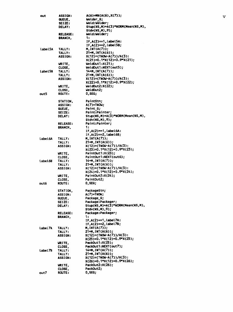
out ASSIGN: QUELJE, SEI 2E: DEUY:
RELEASE : BRANCH,
TALLY: TALLY: ASSIGN:
URITE, CLOSE, TALLY: TALLY: ASSIGN:
URITE, CLOSE, RWfE:
STAT 1 ON, ASSIGN: QUEUE, SEIZE: DELAY:
RELEASE : BRANCH,
TALLY: TALLY: ASSIGW:
URITE, CLOSE, TALLY: TALLY: ASSIGN:
URITE, CLOSE, ROUTE :
STAT 1 ON, ASS 1 GN : QUEUE, SEIZE : DELAY:
RELEASE : BRANCH,
T ALLY: TALLY: ASSIGN:
MI TE, CLOSE, TALLY : TALLY: ASS 1 GN :
VRITE, CLOSE, ROUfE:
Pain tStn ; A(7)=TNOU; Paint-Q; Paint :Painter; St~(NS,M)+AC3)*NORUCMean<wS,n), StdvCNS,M),9); Pa in t zPa in te r ; 1: IF,A(2)=1,labelbA: IF,A(2)=2,LabeLbB; M, INTCAC7)); 21+H,INTCAC611; X(12)=<TNW-A<7))/AC3): x(23~=0*1*X~12)+0.~Xcu) ; P a i n t O u t l :X(231; P a i n t O u t l :NEXT(out6); 14+ü,INT<AC7>); 21+çI,INTCAC6>); X<12)=CT NW-A(7) )/AC31 : X(24)=0*1*XC~2)+0.9*XC24); PaintOut2:XC24); PaintOut2; 0,SEO;
PackageStn; AC7)=TNOV; Package-Q; Package:Packager; S~~~(NS,U)+AC~)*NORMCH~~~CNS,M), StdvCUS,M),91; Package:Patkager; 1: IF,A(2)==l81abel7A: i F,A(Z)==Z, LabeLiB; !t,INTCACI)); 21*, I W f CAC61 ); XC~Z)=CTNOU-A(~))/AC~): ~(25)=0.1 =xc12)+0.~xc251; Packûut1:XCZS); Paclahrt l :NEXT(out?); 14+n,INTCAC7)); 214, fYTCAC6)); x(~ZI=CTNOV-AC~) )/AC31 : x(26)4.1*XC12)+0,PX<26); Packûut2:XCZb); Packûut2; O, SEO;

STAT 1 ON, ExitSystem;
ASSIGN: TALLY: TALLY: ASSIGN:
BRANCH,
ESFTl ASSIGN:
TALLY : TALLY:
ESFT2 ASSIGN:
TALLY: TALLY:
T a r d i n e s s TALLY: TALLY: TALLY: TALLY: BRANCH,
T a r d y ASS1 GN:
NoTardy ASSIGN:
MeanTardy TALLY: TAL LY : CWNT : CWNT: BRANCH,
displ ASSIGN: URITE,
disp3 ASSIGN: URI TE,
CREATE ; delblk DELAY:
URITE, CLOSE,
PlPZinfo: TNOü8A(S),TNOU-AC6),AC8),A(6),X(5)+X(30)+X(31), DA%( 12) ,DAVG(22) ,oAV~<26) ,AC31 : D 1 SPOSE;
7; timef i te:TNW; timef i te:


v i i i ATTRIEIUTES Calso used in ExitSystem stn as tcmp vars) AC1 ) - Job Ytmber AC21 - Part Type A(3) - Batch Size A(&) - Coupment A Release Date A(S) - Conparient Due Date CESFT a l L types) A(6) - Tinre In a t Shop ACT) - l ime In a t s ta t ion (ESFT by type) AC81 - End 1 tm Due Date AC9) - Tardiness A t t r i k r t e AC101 - Caiponent B Release Date
VAR f ABLES X(?) - Total Nuber o f Batches Caiipleted X(2) - Y u i i b e r o f Batches Conpleted THIS Ueek X(3) - Nuiiber o f Batches Coripleted by U S T Ueek X(b) - Job N-r Index X(5) - Parts UIP Pl C l X(6) - Nunbér of Tardy Jobs X(7) - Tenp Variable XC8) - XC9) - ~ ( 1 0 ) - Uhich f i l e t o read Pl jobs frcnn X(1l) - ühich f i l e t o read P2 jobs from X(t2) - LT tenp var iable (used a t a l l stns) X(13) - -th& Adj FT per pa r t a t Ssw Stn (Pl) X(14) - Smoothed A d j FT pr par t a t Saw Stn <PZ) X(15) - Smoothed Adj FT per part a t Shear Stn (Pl) X(16) - Smoothed Adj FT per pa r t a t Shear Stn (PZ) X(17) - Smoothed Adj FT per pa r t a t Brake Stn ( P l ) X(18) - Smothed A d j FT per par t a t Brake Stn (PZ) X(19) - Smoathed Adj FT pet p a r t a t Punch Stn ( P l ) X(20) - Smothed Adj FT per p a r t a t Prrmh Stn (PZ) X(2l) - Smothed Adj F l per p a r t e t ~ e l d S t n (Pl) X(22) - Smoathed Adj Ft per par t a t Ueld Stn (P2) X(23) - knoothed Adj FT per p a r t a t Paint S t n (Pl) X(24) - Smoothed Adj FT per pa r t a t Peint Stn (PZ) X(25) - Smoothed Adj FT per pa r t a t Pack S t n (Pl) X(26) - Smoothed Adj FT per par t a t Pack Stn (P2) XC27) - Smoothed Adj Overall Batch FT f o r P l X(28) - Smoothed A d j Overall Batch FT f o r P2 x(29) - Smothed FT f o r a l 1 jobs <Pl & PZ) X(30) - Parts VIP P l C2 X(31) - Parts UIP P2 C3 X(32) - Parts UIP PZ C4 Stup - Setup Time (defined i n an array) Mean - Process Hean (defined i n an array) Stdv - Process Standard Deviation (defincd in an array)
I n i t i a l i s e Global Variables
CRUTE; ASS 1 GN : X(4)=10:
X(5 )=6OOO: X(10)=1: X(11)=2: X(13)=0-00100635: X(14)=0.0010662: X(15)=0.0011303: X(16)=0.00114: X(lf)=O.OOlt796S: XC18)=0.00132345: XC19)=0.0010228: X(20)=0.001 tOOl5: X~21)=0.00120295 : X(22)=0.0012858: XC23)=0.00081345: X(24)=0.00081025 :

URITE, CLûSE , URITE, CLME, URITE, CLOSE, URfTE, CLOSE, YRfTE, CLOSE, URITE, CLOSE, URITE, CLOSE, URITE, CLOSE, URITE, CLOSE, URITE, CLOSE, YRITE, CLOSE, URI 7 E, CLOSE, URI TE, CLOSE, URITE, CLOSE,
X(25)=0.00116445: Xc26 )=O. 00086335: X(27)=10.6: X<28)=10.6: X(29)=10,5: XC30)=2000: X<31)=6000: XC32)=2000; S a u u i t l :X(13); SaeOut 1 ; Saiiart2:X(14); SawOut2; S h e a r û u t l :XClS); S h e a r a r t l ; Shearûut2:XC 16); Shearûut2; Braket3utl:XClT); B rakeûu t 1; BrakeûutZ:XC18); Brakeûut2; Punchûutl:XC19); Punchûut 1 ; Punchûut2:XC20); PrachOutZ; Ueldoutf :XC21); UeldOut1; WeldOutE:XC22); UeldOut2; P a i n t û u t f :XCU); Pa in tOu t l ; PaintOut2:KCZb); PaintOutZ; P a c k û u t l :X(2S 1; P a c k û u t l ; PackûutZ:X(Z6); PackOutZ: D 1 SPOSE;
8
; Create Type 1 Jobs 8
CREATE , , 36570 ; repeatl DELAY: 7;
READ 8 XC10): AC1 ),AC3),AC4),ACIO),AC8),A(S);
ASSIGN : A C 2 1 4 : M=Enter: X(4 )=X(b)+l: A( 1 )=X(4);
SRANCH, 3: ALüAYS,CLosel,Yes: ALUAYS, Carp l ,No: ALUAYS,CompZ,Wo;
CLosel CLOSE, XC10): UEXTCrepeatl );
Canpl ASSIGN: HS=1 ; DELAY: W < A C 6 ) - T N ~ , 0 ) 8 1 ; ASS 1 GN : X(S)=X(S)+A<3); RWTE: O,SEQ:WKCA(6) 1;
Cofp2 ASSIGN: NS=2; DELAY: WCA(1O)-TUOU,O) ,2; ASSIGN: XC30)=X(30)+A<3); ROUTE: O,SEQ:IIARK(A(6) );
, ; C r e a t e Type 1 t Jobs 8

CREATE,, 36570; repeat2 DEUY: 7;
R m , XC11): AC1 ,Ac3),ACb) ,A<10) A 8 1 ,ACs);
ASSIGN: AC2)=2: M=Enter: X(4)=X(4)+l: ACI)=XCL);
BRANCH, 3: ALWYS,CLose2,Yes: ALUAYS,Ca@,No: A L W S , Coirpri, No;
C 1 ose2 CLOSE, X(11): NOCTC repeat2);
Cal@ ASSIGN: NS=3; DELAY : W(AC4)-TNûU,O),3; ASS 1 GN : X(31 >=XC31 )+A(3); ROUTE : O,SEQ:MRK(AC6));
C a p 4 ASSIGN: )1S=4; DELAY: CiIAXCAC10)-TNOU,0>,6; ASSIGN: XC32>=X<32>+A<3); RQUfE : O,SEQ:EiURK(A(6) );
STAT I OU, ASSIGN: QUEUE, SEIZE: DELAY:
RELEASE: BRANCH,
l a b e l l A TALLY: TALLY: ASS 1 GN :
URITE, CLOSE,
Label 16 TALLY: TALLY: ASSIGN:
URITE, CLOSE,
o u t 1 ROUTE :
STAT I ON, ASSIGU: QUEUE, SEIZE: DELAY:
RELEASE : BRAICH,
t a b e l 2A TALLY: TALLY : ASS 1 GN :
ShearStn ; A( f)=TNW; Shear-Q; Shear :Wach in is t ; StupCNS8M)+A<3)*NORn<nean(MSrH), StdvCNS ,U) ,9); Shear :Mach in is t ; 1 : IF,AC2>==l,labelîA: 1 F8A(2>==2, Label%; M,INTCAC?J); 214, INTCA(6) ); %C~Z)=<TNOW-AC~)) /A(~) : x<15)=0~1=Xc12)+0~9.X(15);

üûITE, CLOSE,
Labe lZB TALLY: TALLY : ASSIGN:
URITE, CLOSE,
out2 ROUfE:
STAT 1 ON, ASSI GN : QüEUE , SEIZE: DELAY:
RELEASE: BRANCH ,
labeL3A TALLY : TALLY: ASSIGN:
URITE, CLOSE,
LabeL3B TALLY i TALLY: ASSIGN:
URITE, CLOSE,
out3 ROUTE :
STATION, ASSIGN: QUEUE, SEIZE: DELAY :
RELEASE : BRANCH,
l a b e l 4 A TALLY: T ALLY : ASS I GN :
URITE, CLOSE ,
L a b e l 4 8 TALLY: TALLY: ASS 1 GIS :
üUITE, CLOSE,
w t 4 ROUTE :
STAT IûN, ASSIGW: BRANCH,
013 QUEUE , Q26 QUEUE,
MTCH ,
S h e a r a t t l :X<15); S h e a n k t l :NEXTCoutZ); lWi, INTCAC7)); 2l+n, INTCAC6)); xC~~)=(TNOU-AC?) )/AC31 : XC16)=0.1~C12)+0.PXC16); ShearûutZ:X(16) ; Shearûut2; O, SEQ;
PunchStn; A(7 )=TNOV; Punch-Q ; Ptmch:Hachin is t ; Stup(NS,U)+A<3)wNORHCUeanCNS,H), Stdv(NS,M) ,9); Puncl t :Uachin is t ; 1: IF,ACZ)=l,tabet4A: 1FtAC2)==2,label4B; U, INTCAC7)); 2 1 H , INT(AC6)); X(l2)=(TNOU-A(7))/A(3): X(19)=0.1*X(l2)+0.PXC19); P u n c h û u t l :XCl9); Punchûutl:WEXT<wt4); 14+M,INT(A(7)); 2 1 W , INTCAC6)); X(lZ)=(TNW-A(?))/A<3): ~ ~ z o ~ = a . i ~ c i 2 ~ + o . ~ ~ c ~ 0 ~ ; Punchûut2:XC20); P u n c h û u t 2; O, SEO;
Ye ldStn ; A(?) =TNW; 1: IF,NS-1.Q.NS==3,Q13: IFtNS=2.0R.NS==4,Q24; C a i p l W :DETACH; Co@& :DE1 ACH ; A(1): 024, s o r t :
so r t TALLY :

dispi!
displ)
out
l a b e l 5 A
labe lSB
o u t 5
Labe M A
Labe l60
o u t 6
B W C H ,
ASSIGN:
ASSIGN:
ASSIGN: QUEUE, SEIZE: DEtAY:
RELEASE : BRANCH,
TALLY: TALLY: ASSIGN:
VRITE, CLOSE, TALLY: TALLY: ASSIGN:
WRITE, CLOSE , ROUTE :
STAT 1 OH, ASSIGN: QUEUE, SEIZE: DELAY:
RELEASE : BRANCH,
TALLY : TALLY: ASS 1 GN:
URITE, CLOSE, T ALLY : TALLY: ASS 1 GN :
VRITE, CLOSE, RWT E:
STAT 1 ON, ASSIGU: Qu=, SEIZE: DELAY:
RELEASE : BRANCH,
l a b e l 7 A TALLY:
XC30)=X(30)-AC3> : X(7)=A(6): D 1 SPOSE;
~(32)=XC32)-AC3) : XC7)=A(6); D 1 SPOSE;
AC6)=MNCAC6) ,XC7)); Uelder-Q; Ye1d:Uelder; StupcNS,M)+A(3)*N0RMCMean(NS,n), st&c~s,n),w; Ue1d:Uelder; 1: IF,A(2)=lrlabeL5A: 1F,A<2)==2,1abeLSB; M, INTCAC7) 1; 2l+U,INTCAC6)); X<~S)=(TNOU-AC?) )/AC31 : X(21 )=O. 1*XC12)+0.9W21); U e l d O u t l :X<Zl); Ue1a)otl :NEXT<outS); MM, I N 1 CAC7)); 21+MrINTCA<6)); X<12)=(TNW-A(7) )/AC31 : x<22)=0.1''X~12)+0.Pxc22~; UelâûutZ:XC22); UeldOut2; O, SEQ;
P a i n t S t n ; AC7)=T NW; P a i n t Q ; P a i n t ~ P a i n t e r ; stupc~s, u)+Ac3)*NORn(nean(NS,n), StdvCNS,M) ,9); P a i n t : P a i n t e r ; 1: 1 F,A<Z)==I, label6A: 1 F,A(2)=2, Lebe168; M, I U T CAC?) 1; Zl+M,INT(AC6)); X(lZ>=(TNW-AC?) )/AC31 : X(U>=O. 1'~~12)+O.PzX(23); P a i n t û u t l :K(231; ~ a i n t O u t l : N E X t ( w t 6 ) ; 14+n,INT(AC7)); 214, INT CAC6)); x C ~ ~ ) = < T W O U - A ( ~ ) ) / A G ) : ~(24)=0.1.3((12)+O.PX<24); PaintOut2:XC24); P e i n t û u t 2 ; O, SEQ;

TALLY: ASSIGN:
URITE, CLOSE,
labe 17ü TALLY : TALLY: ASSI GN :
üRITE8 CLOSE,
out7 ROUTE:
21+M8tNTCA<6)); XCfZ)=CT NW-AC71 )fAC3) : Xc25)=0~1'X<12)+0~9=x~25); Packûutl :KCZS >; P a c k a r t 1 :NMTCout7); 16+U,INTCA(?)); 21+ü, INTCAC6) >; X<12)=CTlOU-A<7))/AC3): X<26)=0.1"X<12)+0.9*XC2rS); Packurt2:XCZo); Pac k m 2 ; 0, SEQ;
STATION,
ASSIGN: TALLY: TALLY: ASSIGN:
ESFTl ASS 1 GN :
TALLY: TALLY:
ESFTZ ASS 1 Gli :
TALLY: 1 ALLY :
Tard iness TALLY: TALLY : TALLY: TALLY: BRANCH,
Tarây ASSIGN:
N o l ardy ASSIGN:
Hean la rdy TALLY: TAL LY: eOUWT: MUWT : BRAWCH,
di s p t ASS 1 GN : UR 1 TE,
d i s @ ASSIGN: URITE,
X(1)=XC1)+1; 7 l+NS, INT CAC6> 1; 13,INTCAC6)); XC12)=TNW-AC6): x ~ 2 9 ) = 0 ~ 1 ~ c l 2 ~ + 0 ~ m c 2 9 ) : A(S)=XC29); 1: 1 F,A(2)==1 ,ESFTI : IF8A(2)==Z,ESFT2;
xiii

CREATE ; delbtk DELAY:
URITE, CLOSE,
7; t imef i Le:TWü; timef i le: NEXT(âeLb1k);
xiv
END ;

Appendix 2
PROJECT, Modified, Rn;
D 1 SCRETE , 2000,10,9,9;
QUEUES: 1,Saw_QRLVF(A(8)): Z,Shear_Q,LVF(AC8) ) : 3,Brake-Q,LVF(AC8) > 4,Puich0,LVF(A(8)): S,Uelder_Q,LVF(AC8) ) : 6,Paint_Q,LVF(A(8)): ?,Package-Q,LVF(AC8)): 8,Caip13Q:

xvi
SEPUENCES: l,,ShearStn&PunchStn& UeldStn&PaintStn& PackageStnEx i tSys tem:
Z,,BrakeStn&üeldStn: 3,,SauStn&ShearStn&
PunchS tnaBrakeS td PaintStngPackageStngExitSysteai;
F 1 LES: 1 ,Data1 ,". ,\SRM\DATAl .rXT1l,SEQ,FREE, IGNORE: 2,Data2,u..\SRn\DATA2.TXT11,SEQ,FREE,IGNOE: ~ , P ~ ~ ~ ~ O , ~ P ~ ~ ~ ~ O . ~ ~ ~ , S E Q , F R E E , I G N O R E : ~,P~~~~O,~~PZ~~~O.TXP,SEQ,FREE,IGUORE: 5, SauOut l , Il.. \SRM\SawPl . TXtlI, SEQ, FREE, I e E : b ,Sa~Ou t2 ,~~ . .\SRH\SawP2ZfXT11,SEQ, FREE, IGNORE: ~,S~~~~~U~~,~..\SRM\S~~~~P~.TXT~~,SEQ,FREE,IGN~RE: 8, ShearOut2, lm.. \SRn\ShearP2.fXT11, SEQ, FREE, IGNûRE : ~ , B ~ ~ ~ ~ ~ U ~ ~ , ~ . . \ S R H \ B ~ ~ ~ ~ P ~ . ~ X T ~ ~ , S E Q , F R E E , I G N ~ R E : l O , B r a k e û ~ t Z , ~ ~ . .\SRn\BrakeP2.TXT11,SEQ,FREE,IGYORE: 11,PwrchOutl,u..\SRn\P~hP11rXT11,SEQ,FREE,IGNORE: I~,P~~C~O~~Z,~~..\SRM\P~~~~P~.~~~~,SEQ,FREE,IGNORE: ~~,U~~~OU~~,~~..\SR~\U~I~PI.T)(~~~,SEQ,FREE,IGNORE: 14,iiel#)ut2, Il. .\SRîî\UeIdP22TXT1s,SEQ, FREE, IGNORE: ~~,P~~~~~U~~,~~..\SRM\P~~~~P~.T%T~~,SEQ,FREE,IGN~RE: 16,PaintOut2,1m..\SRn\PaintP2,r)(T11,SEQ,FREE,IGNORE: ~~,P~C~O~~~,~..\SRU\P~C~P~.TXT~~,SEQ,FREE,~GNORE: ~~,P~C~O~~~,~..\SR~\P~C~PZ.TXT~~,SEQ,FREE,IGN~RE: ~ ~ , P ~ P ~ ~ ~ ~ ~ , ~ P ~ P Z ~ ~ ~ O . ~ X ~ ~ ~ , S E Q , F R E E , X G N O R E : ZO,timefiLe,~..\SRH\timefiCe.txt~,,FREE,;
STORAGES : 1 ,RelDatel : 2,RelDateZ: 3 ,Re lDate ;
RESWRCES: Hach in is t ,b : Me lder : Painter: Packager : Saw: Shear : Brake: P m c h : UeLd: P a i n t : Package;
ARRIVALS: l ,STATIW(BrakcStn),, l , AC1>=1,A(2)=1,A(3)=2000,A(4)=36571,AC5)=36576, A(6>=TWOU,A(7)=TNW,AC81=36585tA(10)=M571, M=l,NS=Z,IS=l:
2,STAf IûUCShearStn), , 1 , AC1)=1,AC2)=1,AC3)=2000,A(4)=36S71,AC5)=S~?6, AC6)=TNW,A(7)=TNOU,A(8)=36585,A(1O)=MS71, M=2,NS=l,IS=l:
3,STATIWCPaintStn), ,1, AC1 )=2,ACZ)=t ,A(3)=2000,A(4)=365m,AC5)=36574, AC6)=TNW ,A(?)=TWOU,A(8)=36581 ,A(10>=36570, U=tS,NS=l,IS=4:
t,STATIOWCPackageStn), ,l, AC1 )=3,AC2)=1 ,AC3)=2OOO~A(b)=MSbP,A(S)=MS~,

DSTATS : 1OiFNRCSaw) ,Sau U t i 1: fOO*NRCShear),Shear U t i l : 10WNRCBrake) ,Brake U t i 1: lOIrNRCPuich),Pmch U t i L: 10fPNRCUeld),Ueld U t i l : lOPNR(Paint),Paint U t i l : lOWNRCPackage),Package UtiL: 1 0OfNRCHachinist)~CRachinist) ,Machinist U t i 1: 100"MRCUelder),Uelder U t i l : lOOfNRCPainter),?ainter U t i l : lOPNRCPackager), Packager U t i 1 : 10PCNRCSaw)+NRCShear)+NR(Brake)
+URCPuich )+NRCUeLd)+NR(Peint)+~R(Package) )/ 7, Shap Avg Ut i 1 : NQCSau-O) ,Saw 0 Length: NQCShear-O) ,Shear Q Length: NQCBrake-Q1,Brake 9 tength: NQCPunch-Q),Punch Q Length: NQCUelder-Q),Uelder Q Lmgth: NQCPaint-Q),Paint Q Length: NQCPackage-Q),Package Q Length: NOCCoiipl3Q),Uatch Q I Length: NQCCaqQ4Q),!îatch Q2 Length: 10~<6)/MXCXC1)81),Percmt Tardy: XCS),ClP1 i n system: XC30),C2 i n system: %<31),P2 in system: XCS)+X<30)+X(31),Total UIP;
TALLIES: 1,Saw FT Type 1: 2, Shear FT T y p e 1 : 3,Brake FT T y p e 1: 4, Pmch FT T y p e 1 : 5,Ueld FT Type 1: 6,Paint FT Type 1: 7,Package FT Type 1: 8,Cl Uait for Match: 9,C2 Uai t f o r Match: 10,C3 Uai t f o r Match: 11,C4 Uai t f o r Match: 12,Type f FT: 13,Overall FT: 14,Type II FT: 15,Saw FT Type II: 16,Shear FT Type t I : 17,Brake FT Type 1 I : 18,P-h FT Type II: 19,Yeld FT Type II: 20,Paint FT Type II: 21,Package FT Type II: 22,Stnl Cm. FT: 23,StnZ Cm. FT: 24 ,S td C m . FT: 2!5,Stn4 Cm. FI: 26,StnS Cun. FT: 27,StM C m . FT: 28,Stn? C m . FT:

î9,Uean Tardimss 1: 30,Mean Tardiness II: 31,Type 1 ESFT: 32,Type II ESFT: 33,OveraL L ESFT: %,No SF Letenessi 35,Uean Tardimss A-: 36,Adj 10% Lateness: 37,FLow Al lwance 1: %,Flow AlLouance II: 39,Adj 20% Lateneçs;
CWNT ERS: 1,Type 1 Parts Finished: 2,Type II Parts Finished: 3,Type 1 Batches Finished: 4,Type 1 I Batches Finished;
OUT WTS: TAVG(3l),,Type 1 ESFT: TAVG(32), ,Type 1 I ESFT: TAVG<33),,0verall ESFT: TAVG(29),,Mean Tardiness 1: TAVG<30),,Uean Tardiness II: TAVG(35), ,Mean T ardiness Avg: TAVG(34),,No SF Lateness: TAvG<36),,Adj 10% Lateness: TAvG(39), ,Adj 20% Lateness: T AVG(37), , Flow AL L owance 1 : TAVG(38),,FLaw Allowance II: DAVGC22), ,Percent Ta*: DAVG(26),,UIP in system: DAVGClZ),,Shop Avg U t i l : TNW, ,End of Rep;
SEEDS: 1,12345,no: 2,23456,no: 3,36567, no: 4,45678,no: 5,56789,110: 6,67890,no: 7,?89Ol ,no: 8,89012,no: 9,90123,no: 10,01234,no;
REPLICATE, 1,36570;

PROJECT , Originat, RU;
D 1 SCRETE, 2000,10,9,9;
VARIABLES: 1: 2: 3: 6: 5: 6: 7: 8: 9: 10 : 11: 12: 13: 14: 15: 16: 17: 18: 19: 20: 21 : 22: 23 : 24: 25 : 26: 27: 28: 29: 30: 31 : 32: StupC4,7) 8
STATl ONS : 1 ,SawStn:

2, ShearStn: 3, BrakeStn: 4, PmchStn: 5,UeldStn: 6,PaintStn: 7, PackageStn: 8,ExitSystem: 9,Enter;
SEWENCES: l,,ShearStn&PrnchStn& UeldStnePaintStn& PackageStn&ExitSystem=
2,,SawStn&BrakeStn&UeLdStn: 3,,ShearStn&PrnchStn&
UeLdStnePaintStni% PackageStnBExitSystem:
4,,SawSt&BrakeStnBUeL&tn;
FILES: l,Datal,B1,.\SRM\DATAl.fXT~l,SEQ,FREE,IGNORE: 2,Data2,B1..\SRn\DATA2.TXT1t,SEQ,FREE,IGNORE: 3,Pl info,~Pl inf0.~~~,SEQ,fREE,tGNûRE: ~ , P ~ ~ ~ ~ O , ~ ~ P ~ ~ ~ ~ O . T X T ~ , S E Q , F R E E , I G N ~ R E : S,SawOutl, IB. ,\SRM\SawPl .TXTUr SEP, FREE, IGNORE: 6, Sauûut2, IB. ,\SRM\SawPZ. T XfBB , SEQ, FREE, 1 GNORE : 7, Shearûutf ,II. .\SRU\ShearPl .fXTBt,SEQ, FREE, i GNORE: B,S~~~~~U~~,~~,.\SRU\S~~~~P~.TXT~~,SEQ,FREE,IGWRE: 9,Brak-1 ,al. .\SRU\BrakefV .TXTBt,SEQ,FREE, IGNORE: ~ ~ , B ~ ~ ~ ~ G U ~ ~ , ~ . . \ S R ~ \ B ~ ~ ~ ~ P ~ ~ T X T ~ ~ , S E Q , F R E E , I G N O R E : ll,PunchOut1,~..\SRM\PmchP1.TXTB1,SEO,FREE,IGNORE: 1 2, Punchout2 , . \ S R ~ \ P M C ~ P ~ fXtIB, SE9 , FREE , 1 GNORE : 13,UeLdOutl,1B,.\Sl~\YetdPl.fXfBt,SEQ,FREE,~GNORE: ~~,U~~~OU~~,~..\SRM\U~~~P~.'FXT~~,SEQ,FREE,IGNORE: 15,PaintOut1,i1..\SRM\PaintP1.lXTm,SEQ,FREE,IGN0RE: 16,PaintOut2,~..\SRH\PaintPZZTXTtB,SEQ,FREE,IGN~E: 17,PackOutl,1B..\SR~\Pa~kP1.TXT~1,SEQ,FREErIGNORE: 18, PackOut2, lm,. \SRM\PackP2 . TXT1l,SEQ, FREE, IGNORE: ~ ~ , P ~ P ~ ~ ~ ~ O , ~ W P ~ ~ ~ ~ O . ~ X ~ I ~ , S E Q , F R E E ~ I G N O R E : 20, timefi Le,". .\SRM\timefi le. txtts,,FREE,;
STORAGES : 1 ,ReLDatef : 2,ReLDateS: 3,RelDates: 4,RelDate4;
RESWRCES: Hachinist,4: iielder: Painter: Packager: Saw: Shear : Brake: Punch : Ueld: Paint: Package;
ARRIVALS: 1 ,STATI ONCSawStn), ,1, A(1)=1 ,A(2)=1 ,A(3)=20OO,AC4>=365?1 ,A(5)=36576, A(6)=TYW,A(7)=fNOU,A(8)=3658S,AC10)=365?1, M=l,NS=Z,IS=l: 2,STATIûNCShearStn), ,1, A(l)=l,AC2)=l,A(3)=2OOO,AC4>=365?l,A(5)=36576, A(6)=TNW,A<7)=TNOU,AC8)=36585,A(10)=365?1, H=Z,NS=l,IS=l: 3,STATIûN(PaintStn), ,1, A(1)=2,AC2)=1,A<3)=2000,ACb)=36570,A(5)=36574, A[6)=TNW,A(n=TNOU,A(8)=36581,AClO)=M5~, M-d,NS=1,ISet: b,STATIûNCPackegeStn), ,1, AC1 )=3,A(2)=1 ,A(3)=2000,A<6)=36569,A(S )=36S?3, AC6)=TNOU,A<7)=TNOU,A~8}=36580,AC10)=36569,

D STATS : lOOWRCSaw),Saw U t i l : lOPNRCShear),Shear U t i l : lOO*NR(Brake),Brake U t i l : 100*NR(Punch) , P m h U t i l : lOPNR(Ue1d) ,Ueld U t i 1: lOPNRCPaint),Paint U t i l : 100*MRCPackage) ,Package U t i 1 : lOPWR(~achinist)/MR(~achinist) , M a c h i n t U t i 1: 10PNR(Uelder),Uelder U t i l : lOPNR(Painter),Painter UtiL: lOO*UR(Packager),Packager U t i l : lOO*CNRCSaw)+NR(Shear)+NR(Brake)
+ ~ ~ < ~ u n c h ) + ~ ~ ( i i e l d ) + ~ ~ ( ~ a i n t )+NRCPackage> )/7, Shop Avg U t i L : NQCSaw-a) , Saw Q Length: NQCShear-0) ,Shear Q Length: NQCBrake-Q),Brake O Length: NQ(Puich-Q),Punch O Length: NQ(Ue1der-O),Uelder O Length: NQCPaint-Q),Paint O Length: NQ(Package_Q),Package Q Length: NQ(Conpl3Q),Uatch 01 Length: NQ(Catp24Q) ,Match Q2 Length : I O ~ X ( 6 ) / ~ ~ X ( I ) , 1 ) , P e r c e n t Tardy: X<S),CIP1 i n System: X(30),C2 in system: X(31),C3P2 in system: X(32),C4 i n system: XCS)+XC30)+X(31)+X(32),Total UIP;
TALLIES: 1 ,Saw FT Type 1 : 2,Shear FT Type 1: 3,Brake FT Type 1: 4 , P m h FT Type 1: 5,UeLd FT Type 1: 6,Paint Ff Type 1: 7,Package FT Type 1 : 8,Cl U e i t f o r Match: 9,CZ Ua i t f o r Hatch: 10,B U a i t f o r Match: 11,Ct i iait fo r Uatch: 12,Type 1 FT: 13,Overall FT: 14,Type II FT: 15,Saw FT Type II: 16,Shear FT Type II: 17,Brake FT Type Ii: 18,Pmch FT Type II: 19,Ueld FT Type II: 20,Paint FT Type II: 21,Packsge FT Type II: 22,Stnl C m . F l : 23,StnZ C m . FT: 24,Sta Cm. FT:

zs,st& km, n: 26,StnS Cun, FT: 27,Stnb Cun. FT: 28,Stn7 C m . FT: 29,Hean Tardiness 1: 30,Mean Tardiness II: 31,Type 1 ESFT: 32,Type II ESFT: 33,ûverall ESFT: 34,Lâteriess: 35,Mean Tardiness Avg: 36,Adj 10% Lateness: 37,Flow ALLowance 1: 38,FLow AtLowance II: 39,Ad j 20% Lateness;
COLINTERS: 1 ,Type 1 Parts Finished: &Type I I Parts Finished: 3,Type 1 Batches Finished: 4,Type I I Batches Finished;
WTPUTS: TAVG<3118,Type 1 ESFT: TAVGC32I8,TYPe I f ESFT: ~~~~(33),,0~erall ESFT: TAVG(29),,Mean Tardiness 1: TAVG(30), ,Mean Tardiness 1 1 : TAVG(35),,Mean Tardiness Avg: TAVG(%),,NO SF Lateness: T~vG(36),,Adj 10% LôteneSS: TAVG<39>,,Adj 20% LatmSS: ~~~~(37),,Flow Allowance 1: TAVG(~~),,F~W ALL0wanCe 11: DAVGC~~), ,Percent Tardy: D A V G < ~ ~ > , , W ~ P in system: DAVGCIZ), ,Sh0p AVg Utf 1: TNW,,End of Rep;
SEEDS : 1,12345,no: 2,23456,no: 3,34567,no: 4,45678,no: 5,56789,no: 6,67890,no: 7,78901 ,no: 8,890t2,no: 9,90123,no: 10,01234,no;
REPLICATE, 1,36570;
END ;

Original Product Set - Calculation of Average Utilisation Level
total available tirne 3360 demand per week 21 O0
1 P l 1 PZ 1 TOTALS 1 setup partslhr part proc total setup partslhr part proc total Total Prod Mach Util Bln mlc U tirne rate lime time t ime rate time time Time %
SBW 60 165 0.36 823.64 60 160 0.38 847.50 1671.14 49.74 shear 40 145 0.41 908.97 50 155 0.39 862.90 1771.87 52.73 brake 35 135 0.44 968.33 40 1 I O 0.55 1185.45 2153.79 64.10 brake punch 15 1 35 0.44 948.33 5 125 0.48 1013.00 1961.33 58.37 weld 30 150 0.40 870.00 30 140 0.43 930.00 1800.00 53.57 pain! 60 175 0.34 780.00 25 160 0.38 812.50 1592.50 47.40 pack 10 115 0.52 1105.65 40 175 0.34 760.00 1865.65 55.53

Modified Product Set - Calculation of Average Utilisation Level
total auailable time 3360 demand per week 2100
1 P l 1 P2 1 TOTALS 1 setup partdhr part proc total setup partslhr part proc total Total Pro( Mach Util Bln mlc time rate t ime t ime t ime rate time time Time %
saw O O 0.00 O. 00 60 160 0.38 847.50 847.50 25.22 shear 40 145 0.41 908.97 50 155 0.39 862,90 1771.87 52.73 brahe 35 135 0.44 968.33 40 110 0.55 1185.45 2153.79 64.10 brake punch 15 135 0.44 948.33 5 125 0.48 1033.00 1961.33 58.37 weld 30 150 0.40 870.00 O O 0.00 0.00 870.00 25.89 paint 60 175 0.34 780.00 25 160 0.38 812.50 1592.50 47.40 pack 10 115 0.52 9105.65 40 175 0.34 760.00 1865.65 55.53
1 i I I I 1 1 1 1 @IF(@MAX(J$S.. ~$12)=~6,~6," '~)

MACRO T r u n c a t e wl w2
MCOLW wl w 2 xl x2 temp te-2 MCONSTAKT yst yend E i rn
copy wl w 2 x1-x2; omit w l = 0 : 3802% 9999,
LET yst=38030 LET yend=38 3 95 LET n=20
DO i=l:n COLY x2 temp; USE xl=yst:yend. LET tm=mean ( t enp ) PRINT tm LET temp2 ( i ) =tm LST yst=yst+730.5 LET yend=yendi730.5
ENDDO
NOTE NOIE ** CHANGE FILE NWE * * NOTE NOTE * * DO NOT f o r g e t tc change file names as necessary ** NOTE

W C R O PI P2Read erase ci-c20 Read 1C:\THESIS\DYNAMIC\~?27\?'IP21XF0.TXT1 cl-CLO. END let c31=cl-c4 let cl2=cl-cl maximuni cl? cl2 c l 3
Rame ci7='1atenesst nzme c12=' ze ro ' name c13='nxaraÿ1 aescribe cl: Sove 'C: \TI.;'3SIS\MINIT...d\Ff PL .MTW ; Repicce. NCTZ NOTE

MACRO Filetext wl w 2
copy wl w2 x1-x2; omit wï=0:38029.9999.
WRITE tsamples.txt' xi x2
NOTE NOTE NOTE NOTE NOTE
NOT f o rge r to change file names as necesscry "
ENDMACRO

Appendix 5 xxvi i i
S I W V - License #510000 Roger Hattar
Sramery for RepLication 1 o f 1
Project: n a d i f i d Set, Coirponent Due Date R u n execution date : 2/27/1997 AMLyst: Rn Mode1 r w i s i o n date: 2/26/199?
Replication ended a t time : 42708.0
TALLY VARIABLES
I d e n t i f i e r Average Var iat ion Minimm Maximm Observations
Saw FT Type 1 Shear FT Type 1 Brake FT Type 1 Punch FT Type 1 Uetd FT Type 1 Paint FT Type 1 Package FT Type 1 Cl Wait f o r Hatch C2 Ua i t for Match C3 Mai t for Match C4 U a i t fo r Match Type I FT OveraL t FT Type II FT Saw FT Type II Shear FT Type II Brake FT Type II Punch FT Type 1 I Veld FT Type II Paint FT Type II Package FT Type II Stnl Cun,FT Stn2 Cun.FT Stn3 Cm.FT StnG Cun.FT StriS Cun.FT S m 6 Cun.FT S t n 7 C m . FT Mean Tardiness 1 Hean Tardiness 11 Type 1 ESFT Type II ESFT Overall ESFT No SF Lateness Mean Tardiness Avg A d j 10% Lateness Flow Allowance 1 Flow AlLouance II A d j 20% Lateness

DISCRETE-CHNGE VARIABLES
Identifier Average Variation Hiniaun Maximrm
Saw Ut i L Shear U t i l Brake U t i L Punch Ut iL Ueid U t i l Paint U t i 1 Package U t i l Wachinist U t i t Uelder Ut i 1 Painter U t i l Packager U t i l Shop Avg U t i l Saw 0 Length Shear Q Length Brake Q Length Punch O Length Uelder Q Length Paint Q Length Package Q Length Match Q1 Length Match QZ ~ength Percent Tardy ClPl i n system C 2 i n system P2 i n system Total UIP
CWNTERS
I d e n t i f i e r Count Limi t
Type 1 Par ts Finished 2444080 I n f i n i t e Type II Parts Finished 2438570 I n f i n i t e Type 1 Batches Finishe 877 I n f i n i t e Type II Batches Finish 876 I n f i n i t e
I d e n t i f i e r Va lue
Type 1 ESFT Type 1 1 ESFT OveraLL ESFT Mean Tardiness 1 Mean Tardiness II Mean Tardiness A v g No SF Lateness A d j 10% Lateness A d j 20% Lateness Flow AlLouance 1 F L o w AL lowance II Percent Tardy UIP in system Shop Avg U t i l End of Rep
Final Value
Execution time: 0.00 minutes. Siru le t ion rm conplete.

SIMAN V - License #9510000 Rager Mattar
Sunnary f o r Repl icat ion 1 o f 1
Project: Uodi f ied Set, End I t e m Due Date R u n executiondate : 2/27/1997 . Analyst: RC(: Uodel revis ion date: 2/27/3997
Repl icat ion ended a t t ime : 42708.0
TALLY VARIABLES
I d e n t i f i e r Average Var iat ion Minimm Maximun Observations
Saw FT Type 1 Shear FT T y p e 1 Brake FT Type 1 Punch FT Type 1 Ueld FT Type 1 Paint FT Type 1 Package FT Type I C l Uai t f o r Match C2 U a i t f o r Match C3 U a i t f o r Match C4 U a i t f o r Match Type 1 FT Overa 1 L FT Type I I FT Saw FT Type II Shear FT Type II Brake FT Type I I Punch FT Type I I UeLd FT Type II Pa in t FT Type I I Package FT Type I I S t n l Cun.FT Stn2 Cun,FT S t r J Cun.FT Stn4 Cun.FT Stn5 Cm. F f Stn6 Cun.FT Stn7 Cm. FT Uean T a r d i n e s s 1 Uean Tardiness II Type 1 ESFT Type II ESFT ûvera l 1 ESFT No SF Lateness Uean Tardiness Avg A d j 10% Lateness FLow Al lowance 1 FLow ALlwance II A d j 20% Lateness

DISCRETE-CHANGE VARIABLES xxxi I d e n t i f i e r Average Var ia t ion Minimm MaXiaun
Saw U t i 1 Shear U t i 1 Erake U t i l Punch Ut iL UeLd Ut i 1 Pain t U t i 1 Package U t i t Machinist U t i l UeLder U t i 1 Painter U t i l Packager UtiC Shop Avg UtiL Saw Q Length Shear Q Length Brake Q Length Pmcb 0 Length Uelder Q Length Paint Q Length Package Q Length Match Q1 Length Match O2 Length Percent Tardy ClP1 i n system C2 in s y s t m PZ in system Total UIP
Iden t i f i e r Count L imi t
Type I Parts Finished 2444080 I n f i n i t e Type I I Parts Finished 2660730 I n f i n i t e Type 1 Batches Finishe 877 f n f i n i t e Type I I Batches F in ish 877 I n f i n i t e
Ident i f ie r Va Lue
Type 1 ESFT Type II ESFT OveralL ESFT Mean Tardiness 1 Mean Tardiness I I Mean Tardiness Avg No SF Lateness A d j 10% Lateness A d j 20% Lateness Flow AlLouance I FLOU Atlowance II Percent Tardy UIP i n system Shop Avg Ut i l End of R e p
Final Value
Execution time: 0.00 minutes, S imi la t ion run coqtete.

S I W V - License 1Y9510000 Roger î la t tar
Surniary f o r Rep l i ce t ion 1 o f 1
Pro ject : O r i g i n a l Set, Ca i ipo rwt Due Date Rm execu t ion date : 2/28/1997 AnaLyst: RH Hadel r e v i s i o n &te: 2/28/1997
RepLicat ion erded a t t i m e : 41343.0
TALLY VARIABLES
I d e n t i f i e r Average Var ia t ion Rinimm Maximm Observations
Saw FT Type 1 Shear F l Type I Brake FT Type 1 Punch Ff Type 1 Uetd n Type I P a i n t FT Type 1 Package FT Type 1 Cl U a i t for Match CZ Ua i t f o r Match C3 Wait f o r Match C4 U a i t f o r Match Type 1 FT Overall FT Type I I FT Saw FT T y p e I I Shear FT Type 11 Brake FT Type 11 Punch FT Type I I Weld FT T y p e I I P a i n t FT Type I I Package FT Type I I S t n l Cun.FT Stn2 Cun.FT Stn3 Cun.FT Stn4 Cm-FT StnS Cun-FT Stnb CULFT Stn7 Cm. FT Uean Tard iness 1 Mean Tardiness I I Type 1 ESFT Type I I ESFT Ovetall ESFT Lateness Mean Tard iness Avg Ad j 10% Lateness Flow AlLouance 1 Flow AL l w a n c e f f Adj 20% Lateness

I den t i f i e r
DISCRETE-CHANGE VARIABLES
Average Variation Minimm Uaximrm Final Value xxxi i i
Saw Ut i 1 Shear U t i l Brake U t i l Punch U t i 1 UeLd U t i l Paint U t i 1 Package U t i l Uachinist U t i l Uelder U t i l Painter U t i l Packager U t i 1 Shop Avg U t i l Sau Q Length Shear Q Length Brake Q Length Punch Q Length Uelder Q Length Paint Q Length Package Q Length Match QI Length Match Q2 Length Percent Tardy C1Pl i n System C2 i n system C3P2 in system C4 i n system Total VIP
65 ,3R 68.680 84.834 76,206 7O.567 62,582 73.285 7 3 . m 70,547 62,582 n.2a5 71.644 -15551 -20818 ,59429 .îà942 . O9099 .O6892 16880
-34529 -23096 48,884 6408.6 3224.5 6962. 0 3960.1 20535.
Iden t i f i e r C m t Limi t
Type 1 Parts Finished 1901020 I n f i n i t e Type II Parts Finished 1896330 I n f i n i t e Type 1 Batches Finishe 682 I n f i n i t e Type II Batches Finish 681 I n f i n i t e
OUTPUTS
Iden t i f i e r Va Lue
Type 1 ESFT Type II ESFT Overalt ESFT Mean tardiness 1 Mean Tardiness II Uean Tardiness Avg Lateness Adiusted Lateness ~ l & AlLwance Flow Allowance Percent t a r e UIP i n system Shop Avg U t i 1 End o f Rep
Execution time: 0.00 minutes. Sinulation run conplete.

S I W V - License #9510000 Roger Hattar xxxiv
Suunary f o r Replicatian 1 of 1
P r o j e t : Or ig inal Set, End Item Due Date Rm execution date : 2/28/1997 Analyst: RM Hodel revis ion date: 2/26/1997
Replication ended a t time : 42708.0
TACLY VARIABLES
I d e n t i f i e r Average Var iat ion Minimun Maximm m e r v a t i o n s
Saw FT Type 1 Shear FT Type 1 Brake FT Type 1 Punch FT Type 1 Ueld FT Type 1 Paint Fl Type 1 Package FT Type 1 Cl Uai t f o r Match C 2 Ua i t for Match C3 Uai t f o r Match C1 Uai t f o r Match Type 1 FT Overal 1 FT Type I I FT Saw FT Type I I Shear FT Type I I Brake FT Type I I Punch FT Typ: I I Ueld FT Type I I Paint FT Type I l Package FT Type II Stn l Cun.FT Stn2 Cun.FT Stn3 Cun.FT Stn4 Cun.FT Stn5 Cm.FT Stn6 Cun.FT Stn7 Cun.FT Mean Tardiness 1 Mean Tardiness I I Type 1 ESFT Type I I ESFT ûvera l l ESFT Lateness Mean Tardiness Avg A d j 10% Lateness Flow A t lowance 1 Flow A l h a n c e I I A d j 20% Lateness

DISCRETE-CWGE VARIABLES
Average Variat ion Mininun lhxiaun F i m l Value XXXV
Saw U t i 1 Shear U t i 1 Brake U t i 1 Punch U t i 1 Yeld Ut iL Paint U t i l Package U t i t Machinist U t i l Ueider U t i l Painter U t i l Packager UtiL Shop Avg U t i l Saw Q Length Shear Q tength Brake P Length Punch Q Length Uelder P Length Paint Q tength Package Q Length Match Q I tength Match Q2 Length Percent Tardy C1P1 i n System C2 in system C3P2 i n system C4 i n system Total Y I P
65.179 68.852 85-05? 76.030 70,495 62.190 73.347 73-??9 70.495 62- 190 73,347 71,593 .l894? -21664 .SE16 .îS9?6 . O9571 . (36671 -16569 .6279l .267l 7 51.152 6919.9 3762.7 7309.3 6624.0 22416.
Iden t i f i e r
100.00 fOO.OO 100.00 t00*00 100.00 100.00 100.00 100.00 900.00 100,oo 100.00 100.00 2.0000 2.0000 7.0000 5 .O000 2.0000 2 .O000 3.0000 6.0000 3.0000 64.062 19TIO. 13590. 189ïû. 14220. 61160.
i m i t
Type 1 Parts Finished 2441830 I n f i n i t e Type I I Parts Finished 2443290 I n f i n i t e Type 1 Batches Finishe 876 I n f i n i t e Type I I Batches Finish 876 I n f i n i t e
Iden t i f i e r Va tue
Type 1 ESFT Type II ESFT ûveral l ESFT Hean Tardiness 1 Mean Tardiness I I Mean Tardiness Avg Lateness Adjusted Lateness Flow Atlwance 1 FLOW ALlwance II Percent Tardy UIP in system Shop Avg U t i l End of R e p
Execution the: 0.00 m imes . Simi let ion tm conplete.

Appendix 6
S I W V - License 29210467 Roger Mattar
Stnmary f o r Repl icat ion 1 o f 1
Project: Experimnt 01 R m execution date : 4/ 3/1997 Analyst: RH Model rev is ion date: 4/ 1/1997
Replication erided a t time : 52823.0
TALLY VARIABLES
Identif i e r Average Var ia t ion niniaun M a x i m Observations
Saw FT Type 1 Shear FT Type 1 Brake FT Type 1 Punch FT Type 1 Ueld FT Type 1 Paint FT Type 1 Package FT Type f Cl Uai t f o r îîatch C2 Uai t f o r Match C3 Uait f o r Match C4 Uait f o r Match Type I FT m e r a l L FT Type I I FT Saw FT Type I I Shear fT Type II Brake FT Type 1 i Punch FT Type II UeLd FT Type II Paint FT Type I I Package FT Type If Stnl Cm.FT StnZ Cm.FT Stn3 Cun.FT Stn4 Cun.FT S t n S Cm-FT Stn6 Cun.FT Stn7 Cm.FT Mean Tardiness 1 Xean f ardiness 1 1 Type 1 ESFT Type I I ESFT Overall ESFT No SF Lateness Mean Tardiness Avg A d j 10% Lateness FLOW AlLwance i FLOU AlLwance II A d j 20% Lateness

Iden t i f i e r
DISCRETE-CHANGE VARIABLES
Average Var iat ion M i n i u m Maximm FinalValue
xxxvi i
Saw U t i l Shear Ut i L Brake U t i t Pmch Uti 1 Ueld U t i l Paint Ut i 1 Package U t i l Machinist U t i 1 Yetder U t i l Painter Ut i 1 Packeger Ut i L Shop Avg U t i l Saw Q Length Shear Q Length Brake 0 Length Punch Q Length YeLder Q Length Paint O Length Package O Length match QI Length Match 02 Length Percent Tardy C1PI i n system C2 i n system PZ i n system Total UIP
I den t i f i e r Count L imi t
Type 1 Parts Finished 6857130 I n f i n i t e Type II Parts Finished 4851190 I n f i n i t e Type 1 Batches Finishe 2321 I n f i n i t e Type 11 Batches Finish 2321 I n f i n i t e
M P U T S
I den t i f i e r Va tue
Type I ESFT Type II ESFT ûveral t ESFT Mean Tardiness 1 Mean Tardiness II Mean Tardiness Avg No SF Lateness A d j 10% Lateness A d j 20% Lateness Flou Allowance Flow AlLowame Percmt Tarây UIP in system Shop Avg U t i l End of Rep
Execution time: 0.00 minutes. Simrlation run conplete.


xxxix

Appendix 8
IDENTIFIER ESTD. MEAN STANDARD -950 C.1. MfNItilOM MAXIMLM NWBER DIFFERENCE DEVIATIûN HALF-VIDTH VALUE VALUE OF OBS
REJECT HO => MANS ARE MOT EQUAL AT -050 LEVEL
HEAN-DIFFEREMCE INTERVALS : EXPO1-VS-EXP03
------------------------------------*-----------------------------------
/ 1 = TEST < O OR 1 ) C = L M R 95% CL X = AVERAGE 1 = UPPER 95% CL 1

x l i

I M A ~ ~ LVALUAIIUN TEST TARGET (QA-3)
APPLIED I W G E . lnc = 1653 East Main Street - -. - - Rochester, NY 14609 USA -- -- - - Phone: 71 W4û2-0300 -- -- - - F a 71 6/28&5989