dynamic toll pricing framework for discrete-time dynamic...
TRANSCRIPT
Dynamic Toll Pricing Framework
for Discrete-Time Dynamic Traffic Assignment Models
Artyom Nahapetyan (corresponding author)
Tel. (352) 392 1464 ex. 2032
Fax: (352) 392 3537
Email address: [email protected]
Center for Applied Optimization, Department of Industrial and Systems Engineering
University of Florida, 303 Weil Hall, P.O. Box 116595, Gainesville, FL 32611-6595
Siriphong Lawphongpanich
Email address: [email protected],
Center for Applied Optimization, Department of Industrial and Systems Engineering
University of Florida, 303 Weil Hall, P.O. Box 116595, Gainesville, FL 32611-6595
September 19, 2006
1

Abstract
This paper discusses a toll pricing framework for a traffic network in a dynamic setting.
The model is based on a discrete-time dynamic traffic assignment problem, where the travel
time is a function of density. We construct a set of time-varying toll vectors such that a
solution (or an approximate solution) of the system problem is a solution of the corresponding
tolled user equilibrium problem. In general, a valid time-varying toll vector is not unique
and the set of valid toll vectors can be expressed algebraically. Then, a desired time-varying
toll vector can be chosen to optimize a secondary objective. Illustrative numerical results
from a small network are provided.
Key words: congestion toll pricing, time-varying tolls, dynamic traffic assignment.
2
1 Introduction
Along with the system optimum (SO) and user equilibrium (UE) problems the congestion toll
pricing problem plays an important role in the road planning and the control of the traffic flows.
Although the solution of the system optimum problem provides the most efficient utilization of
the existing roads, an user equilibrium solution better represents travelers’ behavior because it
assumes that the drivers choose the shortest path in reaching their destination. The toll pricing
problem imposes additional costs on the roads to transform the system optimum solution into
a solution to an user equilibrium problem with tolls (see, e.g., Beckmann (1965) and Dafermos
and Sparrow (1971)). In the literature a toll vector that allows this transformation is often
called a valid toll vector.
In the static traffic assignment models, the travel time is a function of the arc flow, and
toll pricing can be classified as “first-best” or “second-best”. The former assumes that every
road in the network can be tolled, and it is well known that a toll vector based on marginal
social costs is always a valid toll vector. Bergendorff el al. (1997) and Hearn and Ramana (1998)
show that other valid toll vectors exist and describe the set of valid toll vectors algebraically.
In an ideal case, when the travel time function is strictly monotone, and the system optimum
problem is convex, the set of valid toll vectors reduces to a convex cone. The toll set allows
choosing a valid toll vector that optimizes a secondary objective function (e.g., minimizing the
total revenue, maximum toll, or number of toll booths). Yildirim and Hearn (2005) extended
the results for the elastic demand case. Computational methods for such models are discussed
in Hearn et al. (2001), Bai et al. (2004, 2006), and Yildirim and Hearn (2005). If only a subset of
roads is allowed to toll, then usually the set of valid toll vectors is empty. In other words, there
is no a toll vector that transforms a system optimum solution into a solution of the tolled user
3

equilibrium problem. The objective of the second-best problem is to find a toll vector where a
solution of the corresponding tolled user equilibrium problems minimizes the total travel time
as well. Mathematical formulations of the second-best problem are either bilevel optimization
problems or mathematical programs with equilibrium constraints (see, e.g., Labbe et al. (1998),
Ferrari (2002), Brotcorne (2001), Yang and Lam (1996), Patriksson and Rockafellar (2002), and
Lawphongpanich and Hearn (2004)).
Dynamic models assume that travel demand between origin-destination pairs vary over time.
Despite a variety of models proposed for both problems, user equilibrium and system optimum,
few papers address the dynamic toll pricing. Agnew (1977) presents a dynamic model for a
highway and using optimal control theory analyzes marginal costs and associated tolls. Carey
and Srinivasan (1993) derive system marginal costs, user perceived costs and user externality
costs. The authors consider a set of tolls that depend not only on the level of congestion but also
the rate of change of congestion. Using optimal control theory, Huang and Yang (1996) propose a
congestion pricing problem on a network of parallel routes with elastic demand. Another optimal
control formulation of the problem as well as a marginal cost based toll vector is discussed by
Wie and Tobin (1998).
In this paper, we consider the first-best dynamic toll pricing framework similar to the one
developed by Bergendorff el al. (1997) and Hearn and Ramana (1998) for the static case. In par-
ticular, the framework consists of the following steps: (i) solve a system optimum problem, (ii)
derive the set of valid toll vectors for a solution of the problem and (iii) solve a toll pricing prob-
lem with a secondary objective. However, most of the system optimum problems with dynamic
settings are non-convex and can have multiple solutions. Furthermore, finding an exact solution
of a large problem is computationally expensive (see, e.g., Nahapetyan and Lawphongpanich
4
(2006)), and heuristic algorithms provide an approximate solution of the problem. Therefore,
we consider the following problem: given a feasible flow, e.g., an approximate solution to the
system problem, find time-varying tolls that transform it into a tolled user equilibrium solution.
A toll vector inducing a desirable feasible flow is called “flow-inducing” toll vector.
Based on a solution or an approximate solution to the discrete-time dynamic traffic assign-
ment problem from Nahapetyan and Lawphongpanich (2006), we construct a time-expanded
network, which we refer to as reduced time-expanded network (RTE). Using the RTE, we prove
that the feasible solution is in user equilibrium if and only if it is a solution of a linear minimiza-
tion problem associated with the underlying RTE network. By adding tolls to the objective of
the minimization problem and applying LP duality, the set of flow-inducing toll vectors can be
expressed algebraically. When the feasible flow is a system optimum, we show that tolls related
to marginal social costs always induce a system optimum solution.
Although we derive flow-inducing toll vectors using a feasible solution of the discrete-time
dynamic traffic assignment problem from Nahapetyan and Lawphongpanich (2006), a similar
framework can be easily applied to other models as well. In particular given an approximate or
a desirable feasible flow obtained from other models or simulation techniques, one can compute
the travel time, construct an appropriate RTE network, and apply the framework discussed in
this paper.
For the remainder, Section 2 briefly discusses the DTDTA problem. See Nahapetyan and
Lawphongpanich (2006) for more details. Sections 3 and 4 discuss the reduced time-expanded
network and the set of flow-inducing toll vectors, respectively. The toll pricing problems with
different objectives and constraints are presented in Section 5. Some illustrative examples are
provided in the Section 6 and finally, Section 7 concludes the paper.
5
2 Discrete-Time Dynamic Traffic Assignment Problem
In this section, we briefly discuss the discrete-time dynamic traffic assignment problem with a
periodic planning horizon in Nahapetyan and Lawphongpanich (2006). The model considers a
circular planning horizon [0, T ), where 0 and T are the same instant of time (see Figure 1), and
assume that if an event occurs at time t, then the same event also occurs at time t + kT , for all
integer k ≥ 1. Because the planning horizon is circular, events occurring in the next period are
assumed to occur in the same interval that represents the current period. In general, if a car
enters a street at time t1 < T and takes τ < T units of time to traverse, then the two events
are assumed to occur at t1 and modt1 + τ, T on the interval [0, T ). This section presents a
discrete-time version of the problem in which the interval [0, T ) is represented as a set of discrete
points, i.e., ∆ = 0, δ, 2δ, · · · , T − δ, where δ = TN and N is a positive integer.
To formulate the problem, let G(N,A) represent the underlying transportation network
where N and A denote the set of nodes and arcs, respectively. It is convenient to refer to
elements of A either as a single index a or a pair of indices (i, j). The latter is used when it
is necessary to reference the two ends of an arc explicitly. Furthermore, C is a set of origin-
destination (OD) pairs and the travel demand for OD pair k during the time interval [t, t + δ],
t ∈ ∆, is hkt . Although the travel time function associated with each arc, φa, can depend on a
number of factors (see, e.g., Wu et al. (1997), Ran and Boyce (1996), and Carey el al. (2003)), in
this formulation we assume that it depends only on the number of cars on the arc. Furthermore,
φa is continuous, non-decreasing and bounded by T , i.e., 0 < φa(w) < T , ∀w ∈ [0, Ma], where
Ma is a sufficiently large upper bound for the range of φa(w). In particular, φa(0) represents
the free-flow travel time on arc a.
We use the dynamic or time-expanded (TE) network to determine the state of vehicular
6
traffic in the system at each time t ∈ ∆. To construct the TE network, the travel time also
needs to be discretized, and the set of possible discrete travel times of arc a is Γa = s : s =
dφa(w)δ e, 0 ≤ w ≤ Ma. To incorporate the time component in the TE network, every node in
the static network (or static node) is ‘expanded’ or replicated once for each t ∈ ∆. Let it denotes
the corresponding replicate of the node i ∈ N in the TE network. Similarly, each static arc (i, j)
expands into |∆| × |Γ(i,j)| TE arcs of the form (it, j mod (t+s,T )),∀ t ∈ ∆, s ∈ Γ(i,j).
To reference flows on TE arcs, let yka(t,s) denote the amount of flow on corresponding arcs of
the TE network. In particular, if a = (i, j), then the subscript a(t, s) refers to TE arcs of the
form (it, j mod (t+s,T )). To compute the time to traverse a static arc at time t, let
Ωa(t) = (τ, s) : τ = [t− 1]T , [t− 2]T , · · · , [t− s]T , s ∈ Γa .
where
[q]T =
q if q ≥ 0
T + q if q < 0
In words, Ωa(t) contains pairs of entrance, τ , and travel times, s, for static arc a such that, if
a car enters static arc a at time τ and takes s time units to traverse it, the car will still be on
the arc at time t. Using the set Ωa(t), the total number of cars on static arc a at time t or xa(t)
is∑
(τ,s)∈Ωa(t)
∑k∈C yk
a(τ,s). Although the variable xa(t) is eliminated from the formulation of
the problem by substituting the appropriate sums into the corresponding constraints and the
objective function, in the paper we use it to describe explicitly the number of cars on the arc a
at time t.
There are two additional sets of decision variables. One set consists of za(t,s), a binary
variable that equals one if it takes between (s− δ) and s units of time to traverse arc a at time
t. In the formulation below, the value of za(t,s) depends on xa(t) and, for each t, za(t,s) = 1
7
for only one s ∈ Γa. The other set consists of gk, a vector with a component for each node in
the TE network. Component it of gk is set to zero if i is not the destination node of OD pair
k. Otherwise, gkd(k)t
, where d(k) denotes the destination node of the OD pair k, is a decision
variable that represents the amount of flow for commodity k that reaches its destination, d(k),
at time t.
Below is a mathematical formulation of the discrete-time dynamic traffic assignment problem
with periodic planning horizon (DTDTA).
min(y,g,z)
∑
t∈∆
∑
a∈A
φa
∑
(τ,s)∈Ωa(t)
∑
k∈C
yka(τ,s)
∑
s∈Γa
∑
k∈C
yka(t,s)
= Φ(y)T y
subject to:
Byk + gk = bk ∀k ∈ C (1)
∑
t∈∆
gkd(k)t
=∑
t∈∆
hkt ∀k ∈ C (2)
∑
s∈Γa
za(t,s) = 1 ∀t ∈ ∆ and a ∈ A (3)
∑
s∈Γa
φ−1a (s− δ)za(t,s) <
∑
(τ,s)∈Ωa(t)
∑
k∈C
yka(τ,s) ≤
∑
s∈Γa
φ−1a (s)za(t,s) ∀t ∈ ∆ and a ∈ A (4)
∑
k∈C
yka(t,s) ≤ Maza(t,s) ∀t ∈ ∆, a ∈ A and a ∈ Γa (5)
yka(t,s) ≥ 0, gk
d(k)t≥ 0, za(t,s) ∈ 0, 1 ∀t ∈ ∆, a ∈ A, s ∈ Γa and k ∈ C (6)
where y and Φ(y) are vectors of arc flows (yka(t,s)) and travel times (Φa(t)(y) = φa(xa(t)) =
φa(∑
(τ,s)∈Ωa(t)
∑k∈C yk
a(τ,s))) whose components are defined so that their inner product is con-
sistent with the summations.
In the objective function,∑
s∈Γa
∑k∈C yk
a(t,s) represents the number of cars that enter arc a
at time t and, based on our assumption, these cars experience the same travel time, φa(xa(t)).
Thus, the goal of this problem is to minimize the total travel time or delay. In that sense,
DTDTA is a system optimum (SO) problem.
8
Constraint (1) ensures that flows are balanced at each node in the TE network, where B
denotes the node-arc incidence matrix of the TE network and bk is a constant vector with a
component for each TE node. The component of bk are defined as follows:
bkit =
0 if i 6= o(k)
hkt if i = o(k)
where o(k) denotes the origin node of OD pair k. Constraint (2) guarantees that the number of
cars arriving at the destination node d(k) equals the total travel demand of OD pair k during
the planning horizon.
It is easy to show that constraint (4) can be replaced by
∑
s∈Γa
(s− δ)za(t,s) < φa
∑
(τ,s)∈Ωa(t)
∑
k∈C
yka(τ,s)
≤
∑
s∈Γa
sza(t,s).
The latter in combination with constraints (3) and (5) compute the travel time for the cars that
enter arc a at time t and only allow flows to traverse the corresponding arc in the TE network.
In particular, constraint (3), in conjunction with the above inequality, chooses one (discretized)
travel time s ∈ Γa that best approximates Φa(t)(y), i.e., Φa(t)(y) ∈ (s− δ, s]. When a represents
arc (i, j), constraint (5) only allows arc (it, imod(t+s,T )) to have a positive flow. Otherwise, (5)
forces flows on arc (it, imod(t+τ,T )), for τ ∈ Γa and τ 6= s, to be zero. Finally, constraint (6)
makes sure that appropriate decision variables are either nonnegative or binary.
3 Reduced Time-Expanded Network and User Equilibrium So-
lution
In this section, we introduce a reduced time-expanded network constructed based on a given
feasible solution to DTDTA. The network provides a useful tool to check weather the feasible
9
vector is in user equilibrium or not. In particular, we show that a feasible vector is an user
equilibrium solution if and only if it is a solution of a set of shortest path problems constructed
on the reduced time-expanded network.
Let (y, g, z) denote a feasible solution of the DTDTA problem and Φa(t) = Φa(t)(y). For each
pair (a, t), a ∈ A, t ∈ ∆, let sa(t) denote the element from the set Γa such that za(t,sa(t)) = 1.
Observe that za(t,s) = 0, for all s ∈ Γa, s 6= sa(t). As a result, yka(t,s) = 0, ∀s ∈ Γa, s 6= sa(t), and
in the TE network arcs a(t, s), s 6= sa(t), do not have flows. By removing those arcs, i.e., all
arcs a(t, s) such that za(t,s) = 0, we refer to the simplified TE network as reduced TE network
and denote by RTE(z). Notice that the structure of the reduced TE network depends on vector
z, and the network consists of arcs a(t, sa(t)). In the RTE(z) network, there are |∆| copies of
origin and destination nodes, i.e., one copy for each t ∈ ∆. For each OD pair k, let Okt represent
the corresponding copy of the origin node at time t and P k(t) denote the set of paths in the
RTE(z) network that emanate from the Okt node and terminate at the destination node Dk
t′ , for
some t′ ∈ ∆. In addition, let P k represent the set of paths in the static network G(N, A) that
emanate from the origin node and terminate at the destination node of the OD pair k.
Lemma 1 Given a feasible solution to the DTDTA problem, (y, g, z), there is a one-to-one
correspondence between sets P k × ∆ and⋃
t∈∆ P k(t) for all k ∈ C such that the travel time
on path pk of the static network at time t equals to the travel time on the corresponding path
pk(t) ∈ P k(t) in the RTE(z) network.
Proof: Let path pk ∈ P k consist of arcs a1, a2, ... an and t0 ∈ ∆ represent the time to enter
the network. Consider the first arc in the path, a1 = (i, j). Because the travel time on arc a1
is known, the (discrete) time to leave the arc is t1 = t0 + dΦa1(t0)/δe = t0 + sa1(t0). In the TE
network za1(t0,sa1 (t0)) = 1; therefore, arc (it0 , jt1) belongs to the RTE(z) network. Associate arc
10
a1(t0, sa1(t0)) in the RTE(z) network with the pair (a1, t0). Assume that ∀l < m correspondence
between arcs al(tl−1, sal(tl−1)) and pairs (al, tl−1) is established. Consider arc am. From the
assumption it follows that the time to enter the arc is tm−1. The latter implies that the time
to leave the arc is tm = tm−1 + dΦam(tm−1)/δe = tm−1 + sam(tm−1), and zam(tm−1,sam (tm−1)) = 1.
Thus, associate arc am(tm−1, sam(tm−1)) of the RTE(z) with pair (am, tm−1). The described
procedure constructs a path in the RTE(z) network that emanates from the origin node Okt0 and
terminates at a destination node Dkt′ , for some t′ ∈ ∆. Let pk(t0) denote the constructed path,
i.e. pk(t0) = a1(t0, sa1(t0)), . . . , an(tn−1, san(tn−1)). This shows that (pk, t0) corresponds to
pk(t0). Conversely, it is easy to see that pk(t0) also corresponds to (pk, t0). Thus, there is a
one-to-one correspondence between pair (pk, t) and path pk(t). Furthermore, because Φai(ti−1)
represents the travel time on arc a at the time to enter the arc ti−1, the travel time on path pk
at the time to enter the arc t is equal to the travel time on path pk(t) of the RTE(z) network.
¥
From Lemma 1 it follows that given a feasible solution, (y, g, z), one can construct the reduced
TE network and analyze the solution using paths in the RTE(z) network. Although RTE(z)
is a subgraph of the TE network, to some extend it can be viewed as a static network. The
latter makes easier proving some properties of the feasible solution. Because of the one-to-one
correspondence, below we use notation p(t) to describe path p ∈ ⋃k∈C P k at time t in the static
network G(N, A) as well as the corresponding path in the RTE(z) network.
The DTDTA problem discussed in Section 2 is a system optimum problem, where the ob-
jective is to minimize the total delay of all drivers during the time horizon [0, T ). In the user
equilibrium problem, the objective is to find a feasible vector to the DTDTA problem, (y, g, z),
such that all users choose one of the shortest paths among all alternative paths available at
11
the time to enter the network. Given a feasible vector (y, g, z), yka(t,sa(t)) represents the flow on
the arc a(t, sa(t)) of the RTE(z) network that belongs to the OD pair k. Let up(t) denote the
number of cars entering the path p(t) ∈ ⋃k∈C P k(t) during the time interval [t, t + δ). Observe
that up(t) depends on the vector y. Similarly, let Φp(t)(y) represent the travel time on path p(t).
Using these notations, formally the concept of a user equilibrium solution can be defined as
follows:
Definition 1 A feasible vector (y, g, z) of the DTDTA problem is called a dynamic user equi-
librium solution if
up(t)[Φp(t)(y)− πkt ] = 0 ∀k ∈ C, t ∈ ∆ and p(t) ∈ P k(t), (7)
where πkt = minp(t)∈P k(t) Φp(t)(y).
According to the definition, if up(t) > 0 then path p(t) is the shortest one among alterna-
tive paths, i.e., Φp(t)(y) = πkt . On the other hand, if the path is not used, i.e., up(t) = 0, then
Φp(t)(y) ≥ πkt . Although the definition deals with the paths in the RTE(z) network, observe that
by interpreting p(t) as the path p of the static network G(N,A) at the time t, it is similar to other
definitions of the user equilibrium solution in the literature. Given a feasible vector, (y, g, z), the
definition allows to check if it is an user equilibrium solution. In particular, compute the travel
time on all arcs at all discrete times t ∈ ∆, Φa(t)(y) = φa(xa(t)) = φa(∑
(τ,s)∈Ωa(t)
∑k∈C yk
a(τ,s)),
compute the travel times on all paths p at time t, Φp(t)(y), and check if equality (7) is satisfied.
The theorem below provides an alternative way to check if a feasible vector is an user equilib-
rium solution. The procedure involves solving the following minimization problem, where the
underlying network is RTE(z).
12
SP (y, z):
minu
ΦT u
subject to∑
p(t)∈P k(t)
up(t) = htk ∀k ∈ C and t ∈ ∆
up(t) ≥ 0 ∀k ∈ C, t ∈ ∆ and p(t) ∈ P k(t)
where Φ and u are the vectors of Φp(t)(y) and up(t), respectively. Observe that the problem can
be decomposed into |C||∆| problems, i.e., one problem for each pair (k, t) ∈ C × ∆, where t
is a (discrete) time to enter the network. In addition, note that each decomposed problem is
equivalent to finding a shortest path from node Okt to one of the copies of the destination node of
the same OD pair k. Although the above problem is formulated based on the RTE(z) network,
SP (y, z) is an ordinary shortest path problem with path costs Φp(t)(y).
Theorem 1 Given a feasible solution to DTDTA, (y, g, z), up(t) satisfies (7) if and only if it is
an optimal solution of the corresponding SP (y, z) problem.
Proof: Observe that SP (y, z) is a linear problem. If πkt denotes the dual variable of the
first constraint of SP (y, z) then the statement of the theorem follows directly from the comple-
mentarity theorem in LP. ¥
According to the theorem, given a feasible solution (y, g, z), we can check if up(t) solves
the SP (y, z) problem. The result confirms or rejects the assumption that (y, g, z) is an user
equilibrium solution. The SP (y, z) problem requires enumerating all paths in the network. To
overcome this difficulty, consider the following alternative arc based formulation instead.
SP (y, z)-A:
miny,g
ΦT∑
k∈C
yk
subject to Bzyk + gk = bk ∀k ∈ C
13
∑
t∈∆
gkd(k)t
=∑
t∈∆
hkt ∀k ∈ C
yka(t,sa(t)) ≥ 0, gk
d(k)t≥ 0 ∀k ∈ C, a ∈ A and t ∈ ∆
where Bz is the node-arc incident matrix of RTE(z), and Φ and yk are the vectors of Φa(t)(y)
and yka(t,sa(t)), respectively. Using the arc based formulation, Theorem 1 can be restated as
follows.
Corollary 1 A feasible vector (y, g, z) is an user equilibrium solution if and only if yka(t,sa(t)) is
an optimal solution of the corresponding SP (y, z)-A problem.
4 Time-Varying Toll Set
In the user equilibrium problem, the solution consists of traffic flows such that each driver
utilizes the shortest path among alternative paths available at the time to enter the network.
On the other hand an optimal solution of the system optimum problem, i.e., the solution of the
DTDTA problem, minimizes the total travel time of all drivers during the time horizon [0, T ). It
is well known that the system and the user equilibrium problems may not have the same solution.
Although the system solution is more efficient than one provided by the user equilibrium problem,
the latter is more realistic in the traffic networks. The toll pricing framework considers charging
additional costs on the arcs, i.e., tolls converted into time units, such that the system optimum
solution is a solution of the tolled user equilibrium problem. The latter is an user equilibrium
problem, where the arc costs include tolls in addition to the travel times. The concept of the
reduced time-expanded network and the theoretical results from Section 3 allow developing a
toll pricing framework similar to the static case (see Hearn and Ramana (1998) and Bergendorff
el al. (1997)).
14
Let (y, g, z) and β denote a feasible solution of the DTDTA problem and a toll vector,
respectively. We refer to the vector β as a y-inducing toll if (y, g, z) is a solution of the tolled
user equilibrium problem. Consider the following problem:
SP (y, z, β)-A:
miny,g
(Φ + β)T∑
k∈C
yk
subject to Bzyk + gk = bk ∀k ∈ C (8)
∑
t∈∆
gkd(k)t
=∑
t∈∆
hkt ∀k ∈ C (9)
yka(t,sa(t)) ≥ 0, gk
d(k)t≥ 0 ∀k ∈ C, a ∈ A and t ∈ ∆ (10)
where the feasible region is the same as in the problem SP (y, z)-A and the objective function
includes the toll vector β in addition to the travel time. The following corollary is a direct
consequence of Corollary 1.
Corollary 2 Given a feasible vector (y, g, z), vector β is a y-inducing toll if and only if (y, g)
is an optimal solution of the corresponding SP (y, z, β)-A problem.
Theorem 2 Given a feasible vector (y, g, z), β is a y-inducing toll if and only if there are vectors
ρk and γ such that
∑
k∈C
[(bk)T ρk + γk
∑
t∈∆
hkt
]= (Φ + β)T
∑
k∈C
yk (11)
BTz ρk ≤ Φ + β ∀k ∈ C (12)
ρkd(k)t
≤ γk ∀k ∈ C and t ∈ ∆ (13)
Proof: Consider the dual problem of SP (z, g, β)-A, i.e.,
maxρ,γ
∑
k∈C
[(bk)T ρk + γk
∑
t∈∆
hkt
]
15
BTz ρk ≤ Φ + β ∀k ∈ C
ρkd(k)t
− γk ≤ 0 ∀k ∈ C and t ∈ ∆
where ρk represents the vector of dual variables of corresponding node conservation constrains
(8), and γk are the dual variables of the constraints (9). From Corollary 2 it follows that vector
β is a y-inducing toll if and only if (y, g) is a solution of the SP (y, z, β)-A problem. Observe that
(y, g) is feasible to the problem. Using the duality theory, vector (y, g) is an optimal solution of
SP (y, z, β)-A if and only if there are vectors ρk and γ feasible to equations (11)-(13). ¥
Theorem 2 provides an algebraic description of the y-inducing toll set. In particular, given
a feasible vector (y, g, z), equations (11)-(13) describe the set of y-inducing tolls associated with
triplet (y, g, z). Using the set, secondary toll pricing problems can be formulated. Observe that
for all feasible vectors (y, g, z), β = −Φ ≤ 0 is a y-inducing toll vector, i.e., the y-inducing toll
set is not empty.
Let (y∗, g∗, z∗) and RTE(z∗) denote the system optimum solution, i.e., the solution of the
DTDTA problem, and the corresponding reduced time-expanded network, respectively. Define
Θa(t) =
(τ, s) : (τ, s) ∈ Ωa(t), z∗a(τ,s) = 1
. In words, Θa(t) is a subset of Ωa(t) such that arc
a(τ, s) remains in the RTE(z∗) network. Because RTE(z∗) consists of arcs of the form a(t, s∗a(t)),
Θa(t) =(τ, s∗a(τ)) : (τ, s∗a(τ)) ∈ Ωa(t)
. In addition, given z∗ compute the lower and the upper
bounds in the equation (4), i.e., L∗a(t) =∑
s∈Γaφ−1
a (s− δ)z∗a(t,s) and U∗a(t) =
∑s∈Γa
φ−1a (s)z∗a(t,s).
Consider the following optimization problem with the underlying RTE(z∗) network structure.
DTDTA(z∗) :
min(y,g)
∑
t∈∆
∑
a∈A
φa
∑
(τ,s∗a(τ))∈Θa(t)
∑
k∈C
yka(τ,s∗a(τ))
∑
k∈C
yka(t,s∗a(t))
= ΦT (y)y
subject to Bz∗yk + gk = bk ∀k ∈ C (14)
16
∑
t∈∆
gkd(k)t
=∑
t∈∆
hkt ∀k ∈ C (15)
L∗a(t) ≤∑
(τ,s∗a(τ))∈Θa(t)
∑
k∈C
yka(τ,s∗a(τ)) ≤ U∗
a(t) ∀t ∈ ∆ and a ∈ A (16)
yka(t,s∗a(t)) ≥ 0, gk
d(k)t≥ 0, ∀t ∈ ∆, a ∈ A, and k ∈ C (17)
where Bz∗ denotes the node-arc incident matrix of the RTE(z∗) network and the vector yk
consists of components yka(t,s∗a(t)). In words, problem DTDTA(z∗) is the DTDTA problem,
where the vector z is fixed to the value of the vector z∗. As we have mentioned above, β∗ = −Φ∗
is a y∗-inducing toll vector. The theorem below proves the existence of another y∗-inducing toll
vector.
Theorem 3 Given a system optimum solution (y∗, g∗, z∗), vector βMSC with components
βMSCa(t,s∗a(t)) =
∑
r∈∆|(t,s∗a(t))∈Θa(r)
[∇xa(r)
φa(r)(x∗a(r))
∑
k∈C
y∗ka(r,s∗a(r)) + λ∗a(r) − µ∗a(r)
](18)
is a y∗-inducing toll vector, where x∗a(t) represents the optimal number of cars on arc a at time
t, λ∗ and µ∗ are the dual multipliers of inequalities (16), and λ∗a(t)µ∗a(t) = 0, ∀a ∈ A and t ∈ ∆.
Proof: Observe that from optimality of (y∗, g∗, z∗) in the DTDTA problem it follows that
(y∗, g∗) is an optimal solution of the DTDTA(z∗) problem. From the KKT sufficient conditions
of the DTDTA(z∗) problem it follows that
Φa(t)(y∗) +
∑
r∈∆|(t,s∗a(t))∈Θa(r)
[∇yk
a(t,s∗a(t))Φa(r)(y
∗)∑
k∈C
y∗ka(r,s∗a(r)) + λ∗a(r) − µ∗a(r)
]
+ρ∗ik − ρ∗jk − ζ∗ka(t,s∗a(t)) = 0,
ζ∗ka(t,sa(t))y∗ka(t,sa(t)) = 0, and ζ∗ka(t,sa(t)) ≥ 0
where vectors ρ∗, λ∗, µ∗, and ζ∗ are the dual variables of corresponding constraints (14), (16),
and (17), and i and j denote the tail and the head nodes of the arc a(t, s∗a(t)), respectively. As
17

a result, if y∗ka(t,s∗a(t)) > 0 then ζ∗ka(t,s∗a(t)) = 0 and
Φa(t)(y∗) +
∑
r∈∆|(t,s∗a(t))∈Θa(r)
[∇yk
a(t,s∗a(t))Φa(r)(y
∗)∑
k∈C
y∗ka(r,s∗a(r)) + λ∗a(r) − µ∗a(r)
]= ρ∗jk − ρ∗ik
On the other hand, if y∗ka(t,s∗a(t)) = 0 then
Φa(t)(y∗) +
∑
r∈∆|(t,s∗a(t))∈Θa(r)
[∇yk
a(t,s∗a(t))Φa(r)(y
∗)∑
k∈C
y∗ka(r,s∗a(r)) + λ∗a(r) − µ∗a(r)
]≥ ρ∗jk − ρ∗ik
Let βMSCa(t,s∗a(t)) =
∑r∈∆|(t,s∗a(t))∈Θa(r)
[∇yk
a(t,s∗a(t))Φa(r)(y∗)
∑k∈C y∗ka(r,s∗a(r)) + λ∗a(r) − µ∗a(r)
]and βMSC
denote the vector of βMSCa(t,s∗a(t)). By viewing the dual multiplies ρ∗ik as potentials of the nodes in
the RTE(z∗) network, it is easy to show that βMSC is a y∗-inducing toll vector; i.e., (y∗, g∗) is
an optimum solution of SP (y∗, z∗, βMSC)-A. In addition, if r ∈ ∆ is such that (t, s∗a(t)) ∈ Θa(r)
then ∇yk′
a(t,s∗a(t))
Φa(r)(y∗) = ∇yk′′
a(t,s∗a(t))
Φa(r)(y∗) = ∇xa(r)φa(r)
(x∗a(t)
), ∀k′ and k′′ ∈ C, k′ 6= k′′.
From the KKT condition it also follows that
µ∗a(t)
L∗a(t) −
∑
(τ,s∗a(τ))∈Θa(t)
∑
k∈C
y∗ka(τ,s∗a(τ))
= 0, and λ∗a(t)
∑
(τ,s∗a(τ))∈Θa(t)
∑
k∈C
y∗ka(τ,s∗a(τ)) − U∗a(t)
= 0.
Observe that at optimality either
∑
(τ,s∗a(τ))∈Θa(t)
∑
k∈C
y∗ka(τ,s∗a(τ)) 6= L∗a(t) or∑
(τ,s∗a(τ))∈Θa(t)
∑
k∈C
y∗ka(τ,s∗a(τ)) 6= U∗a(t).
As a result, at least on of the multipliers is zero, i.e., µ∗a(t)λ∗a(t) = 0. ¥
Because βMSC is a y∗-inducing toll vector; i.e., (y∗, g∗) is a solution of SP (y∗, z∗, βMSC),
from Theorem 2 it follows that there are vectors ρ∗ and γ∗ such that the system
∑
k∈C
[(bk)T ρ∗k + γ∗k
∑
t∈∆
hkt
]= (Φ∗ + βMSC)T
∑
k∈C
y∗k
BTz∗ρ
∗k ≤ Φ∗ + βMSC ∀k ∈ C
ρ∗kd(k)t≤ γ∗k ∀k ∈ C and t ∈ ∆
18

is satisfied. On the other hand, the above system follows directly from the KKT conditions of the
DTDTA(z∗) problem, and corresponding dual variables ρ∗ and γ∗ satisfy the system. However,
observe that (βMSC , ρ∗, γ∗) is not the only solution of the system. In particular (−Φ∗, 0, 0) also
satisfies the system, and β = −Φ∗ is another y∗-inducing toll vector.
The toll vector in Theorem 3 is similar to one obtained from the marginal social cost price
in the static case. In particular, the first component of the toll vector, i.e.,
∑
r∈∆|(t,s∗a(t))∈Θa(r)
[∇xa(r)
φa(r)(x∗a(r))
∑
k∈C
y∗ka(r,s∗a(r))
],
measures the total benefit that is experienced by drivers who enter the arc after time t. In
addition, observe that λ∗a(r) and µ∗a(r) are the dual variables of the inequalities (16), and they
represent the changes in the objective function value in the presence of minor perturbations of
the values of U∗a(t) and L∗a(t), respectively. However, to change the values of U∗
a(t) or L∗a(t), the
binary variable z∗a(t,s) should be changed as well, and the resulting vector may not be feasible or
optimal. In that sense, the second component of the toll vector, i.e,
∑
r∈∆|(t,s∗a(t))∈Θa(r)
[λ∗a(r) − µ∗a(r)
],
measures the cost to maintain the (optimal) network structure of RTE(z∗).
5 Dynamic Toll Pricing Problems
Given a feasible vector to DTDTA, (y, g, z), let =(y, g, z) denote the set of β, ρ, and γ that
are feasible to the system (11)-(13). In the previous section, we have shown that (−Φ, 0, 0) ∈
=(y, g, z) for all vectors (y, g, z) feasible to the DTDTA. In the case of the system solution, i.e.,
(y, g, z) = (y∗, g∗, z∗), Theorem 3 provides another y∗-inducing toll vector; therefore, there are
at least two vectors in the set =(y∗, g∗, z∗). The latter suggests developing toll pricing problems
19
with a secondary objective, where the underlying feasible region is constructed based on the set
=(y∗, g∗, z∗). For instance, a traffic management might be interested in minimizing the total
operating cost, costs of constructing a proper infrastructure (e.g., constructing toll boothes), or
minimizing/maximizing the total revenue. Although the problems below are constructed based
on a system solution (y∗, g∗, z∗), a similar framework applies to an approximate solution or a
feasible vector to the DTDTA problem.
Let κopa(t) and κinf
a denote binary variables such that
κopa(t) =
1 if |βa(t,s∗a(t))| > 0
0 if |βa(t,s∗a(t))| = 0, and κinf
a =
1 if∑t∈∆
|βa(t,s∗a(t))| > 0
0 if∑t∈∆
|βa(t,s∗a(t))| = 0.
Using these variables, consider the following optimization problem to minimize the total oper-
ating and infrastructure costs.
min(β,ρ,γ,κop,κinf )
(cop)T κop + (cinf )T κinf
subject to (β, ρ, γ) ∈ =(y∗, g∗, z∗)
|βa(t,s∗a(t))| ≤ Mκopa(t) ∀a ∈ A and t ∈ ∆
κopa(t) ≤ κinf
a ∀a ∈ A and t ∈ ∆
κopa(t) and κinf
a ∈ 0, 1, ∀a ∈ A, and t ∈ ∆
where cop and cinf are the vectors of operating and infrastructure costs, respectively, and M is
a sufficiently large number. The optimization problem below minimizes the total revenue.
min(β,ρ,γ)∈=(y∗,g∗,z∗)
yT β
Observe that in the above two problems there is no additional requirements on the set of
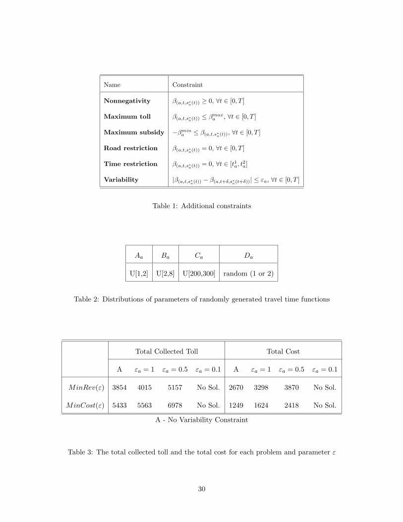
y∗-inducing tolls. However, it might be more desirable to add some constraints from Table 1. In
20
particular, adding the nonnegativity and/or maximum toll constraints prevent from charging a
negative and/or an unrealistically large toll, respectively. If the tolls are allowed to be negative;
i.e., it is allowed to subsidy the drivers on particular arcs, then the maximum subsidy constraint
prevent from paying large amount of money to the drivers. The road and time restriction
constraints prevent from tolling certain roads at certain times of the time horizon, e.g., from
1:00 am to 5:00 am. Finally, the variability constraint restricts the variation of the toll during
the planning horizon. It is noticed that adding those constraints may be too restrictive and
violate the feasibility of the toll set. In such cases the second best pricing problem should be
considered.
6 Illustrative Examples
The toll pricing framework consists of the following steps: (i) solve the DTDTA problem to find
a system optimum solution, (ii) derive the set of flow-inducing tolls, i.e., the set of tolls such
that the system optimum solution is a solution of the tolled user equilibrium problem, and (iii)
solve a toll pricing problem with a secondary objective. Although the DTDTA problem belongs
to the class of nonlinear mixed integer problems that are hard to solve, the set of flow-inducing
toll vectors can be constructed based on any feasible solution; therefore, it is not necessary to
find an exact solution to the DTDTA problem. To find an approximate solution, in the examples
below first we solve a linear mixed integer upper bound problem and then improve the solution
by solving a continuous nonlinear refinement problem. The discussion on those problems is out
of scopes of this paper, and for details we refer to the paper Nahapetyan and Lawphongpanich
(2006). In this section, the approximate solution is used to construct a flow-inducing toll set,
and we consider several examples of toll pricing problems based on the set and some of the
21

constraints from Table 1.
All experiments are conducted on the 9-node network (see Figure 2), which has four OD
pars: (1,8), (1,9), (2,8), and (2,9). In the problems, the time horizon is [0, 30), and δ = 1, i.e.,
∆ = 0, 1, . . . , 29. In addition, the travel time functions are generated according to the formula
φa(xa(t)) = Aa + Ba(xa(t)/Ca)Da , where parameters Aa, Ba, Ca and Da, are random numbers
(see Table 2). To imitate a congestion on the arcs, for each OD pair a demand is generated
according to the formula hkt = 1.1αtζ, where the value of αt depends on time t (see Figure 3), and
ζ is a number uniformly generated from the interval [20, 30]. As a result, the demand gradually
increases during the time interval [0, 9], remains on the same high level during the next 10 units
of time, and then decreases to the initial level at the end of the planning horizon. Note that
according to the formula the demand varies from ζ to 2.36ζ. As it was mentioned above, we find
an approximate solution of the problem by solving the upper bound problem and the refinement
problem. Let (y∗, g∗, z∗) and =(y∗, g∗, z∗) denote the obtained solution and corresponding set
of y∗-inducing tolls, respectively.
One of the toll pricing problems minimizes the total collected toll, subject to the set of y∗-
inducing toll vectors =(y∗, g∗, z∗) and additional nonnegativity and variability constraints. Below
is the mathematical formulation of the resulting problem, which we refer to as MinRev(ε).
min(β,ρ,γ)
y∗T β
subject to (β, ρ, γ) ∈ =(y∗, g∗, z∗)
−εa ≤ β(a,t,s∗a(t)) − β(a,t+δ,s∗a(t+δ)) ≤ εa ∀a ∈ A and t ∈ [0, T ]
β ≥ 0
In the numerical experiments we solve the problem without the variability constraints as well
22
as with variability constraints, where ε = 1, 0.5, or 0.1.
Similarly consider minimizing the total cost subject to the same nonnegativity and variability
constraints. In the experiments, the costs cop and cinf are randomly generated from the intervals
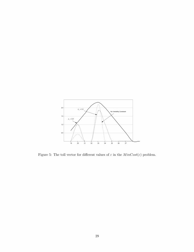
[5, 10] and [100, 150], respectively. We refer to the resulting problem as MinCost(ε).
min(β,ρ,γ,κop,κinf )
(cop)T κop + (cinf )T κinf
subject to (β, ρ, γ) ∈ =(y∗, g∗, z∗)
−εa ≤ β(a,t,s∗a(t)) − β(a,t+δ,s∗a(t+δ)) ≤ εa ∀a ∈ A and t ∈ [0, T ]
βa(t,s∗a(t)) ≤ Mκopa(t) ∀a ∈ A and t ∈ ∆
κopa(t) ≤ κinf
a ∀a ∈ A and t ∈ ∆
β ≥ 0, κopa(t), κ
infa ∈ 0, 1, ∀a ∈ A, and t ∈ ∆
In both problems, at optimality the total collected toll as well as the total cost are computed
(see Table 3). Observe that in both problems the objective function value increases with the
decrease of the value of ε. In the case of ε = 0.1, the variability constraints are too restrictive,
and there is no a nonnegative y∗-inducing toll vector that satisfies the constraints. Table 4
describes the number of toll collecting centers that are necessary to build. Figures 4 and 5
illustrate the influence of the variability constraint on the optimal toll vector. In particular,
the figures illustrate the changes in the toll on the arc (6, 9) during the time interval [19, 28].
Observe that in the case of εa = 0.5 the toll vector is smoother than in other two cases.
7 Concluding Remarks
In the paper, we have developed a toll pricing framework for the discrete-time dynamic traffic
assignment problem. One of the key components of the framework is the reduced time-expanded
23
network, which can be constructed based on an optimal as well as an approximate solutions of
the DTDTA problem. The set of flow-inducing tolls is derived with respect to an optimal
(approximate) solution.
Ideally one would like to construct the set of flow-inducing tolls and the corresponding toll
pricing problems with respect to an optimal solution of the DTDTA problem. However, the
latter belongs to the class of nonlinear mixed integer program, and it is hard to find an exact
solution of the problem. Section 6 discusses several examples of toll pricing problems based on
an approximate solution, which is obtained using the technique discussed in Nahapetyan and
Lawphongpanich (2006).
Although the toll pricing framework is based on an optimal (approximate) solution of DT-
DTA problem, it can be applied to a solution of other system optimum problems or a desirable
feasible flow obtained by simulation techniques. In particular, given a desirable flow y∗, compute
travel time on the arcs at each discrete time t ∈ ∆, construct the corresponding RTE network,
derive the set of y∗-inducing tolls using equations (11)-(13), i.e., the set =(y∗), and solve a toll
pricing problem base on the set =(y∗).
References
Agnew, C.E., 1977. The theory of congestion tolls. Journal of Regional Science 17(3), pp. 381-
393.
Bai, L., Hearn, D., Lawphongpanich, S., 2004. Decomposition Techniques for the Minimum Toll
Revenue Problem. Networks 44(2), pp. 142-150.
Bai, L., Hearn, D., Lawphongpanich, S., 2006. Relaxed Toll Sets for Congestion Pricing Prob-
24

lems. Mathematicl and Computational Models for Congestion Charging, Springer, New York.
Beckmann, M., 1965. On Optimal Tolls for Highways, Tunnels and Bridges. In: Vehicular Traffic
Science, American Elsevier, New York, pp. 331-341.
Bergendorff, P., Hearn, D., Ramana, M., 1997. Congestion Toll Pricing of Traffic Networks.
Network Optimization, Springer-Verlag series, Lecture Notes in Economics and Mathematical
Systems, pp. 51-71.
Brotcorne, L., Labbe, M., Marcotte, P., Savard, G., 2001. A Bilevel Model for Toll Optimization
on a Multicommodity Transportation Network. Transportation Science 35(4), pp. 345-358.
Carey, M., Ge, Y., McCartney, M., 2003. A Whole-Link Travel-Time Model with Desirable
Properties. Transportation Science 37(1), pp. 83-96.
Carey, M., Srinivasan, A., 1993. Externalities, average and marginal costs, and tolls on congested
networks with time-varying flows. Operations Research 41(1), pp. 217-231.
Dafermos, S., Sparrow, F., 1971. Optimal Resource Allocation and Toll Patterns in User-
Optimized Transportation Network. Journal of Transportation Economics and Policy 5, pp.
198-200.
Ferrari, P., 2002. Road network toll pricing and social welfare. Transportation Research Part B
36(5), pp. 471-483.
Florian, M., Hearn, D., 1999. Network Equilibrium and Pricing. Handbook of Transportation
Science, Kluwer Academic Publishers, pp. 361-393.
Hearn, D., Ramana, M., 1998. Solving Congestion Toll Pricing Models. Equilibrium and Ad-
vanced Transportation Modeling, Kluwer Academic Publishers, pp. 109-124.
25
Hearn, D., Yildirim, M., Romana M., Bai L., 2001. Computational Methods for Congestion
Toll Pricing Models. Proceedings of IEEE Conference on Itelligent Transportation Systems,
Berkeley, pp. 257-262.
Huang, H.J., Yang, H., 1996. Optimal variable road-use pricing on a congested network of
parallel routes with elastic demand. Proceedings of the 13th International Symposium on the
Theory of Trafc Flow and Transportation, Lyon , France, pp. 479-500.
Labbe, M., Marcotte, P., Savard, G., 1998. A bilevel model of taxation and its application to
optimal highway pricing. Management Science 44(12), pp. 16081622.
Lawphongpanich, S., Hearn, D., 2004. An MPEC Approach to Second Best Toll Pricing. Math-
ematical Programming 101(1), pp. 33-55.
Nahapetyan, A., Lawphongpanich, S., 2006. Discrete-Time Dynamic Traffic Assignment Model
with Periodic Planning Horizon: System Optimum. Journal of Global Optimization, in press.
Patriksson, M., Rockafellar, R.T., 2002. A Mathematical Model and Descent Algorithm for
Bilevel Traffic Management. Transportation Science 36(3), pp. 271291.
Ran, B., Boyce, D., 1996. Modeling Dynamic Transportation Networks, Springer.
Wu, J., Chen, Y., Florian, M., 1997. The Continuous Dynamic Network Loading Problem: a
Mathematical Fromulation and Solutions Methods. Transportation Research Part B 32(3),
pp. 173-187.
Wie, B., Tobin, R., 1998. Dynamic congestion pricing models for general traffic networks. Trans-
portation Research B 32(5), pp. 313-327.
26
Yang, H., Lam, W.H.K., 1996. Optimal road tolls under conditions of queuing and congestion.
Transportation Research PArt A 30(5), pp. 319332.
Yildirim, M., Hearn, D., 2005. A first best toll pricing framework for variable demand traffic
assignment problems . Transportation Research Part B 39(8), pp. 659-678.
27

0 T
vs
1t
2t
t
0/T
1t
2t
Figure 1: Events occurring in two consecutive planning horizons.
1
2
3
4
6
7
8
9
5
Figure 2: 9-node network.
0 2 4 6 8 10 12 14 16 18 20 22 24 26 28
2
4
6
8
10
tα
t
Figure 3: The value of αt.
19 20 21 22 23 24 25 26 27
0.5
1.0
1.5
2.0
No Variability Constraint
0.1=a
ε
5.0=a
ε
Figure 4: The toll vector for different values of ε in the MinRev(ε) problem.
28
19 20 21 22 23 24 25 26 27
0.5
1.0
1.5
2.0
No Variability Constraint
0.1=a
ε
5.0=a
ε
Figure 5: The toll vector for different values of ε in the MinCost(ε) problem.
29
Name Constraint
Nonnegativity β(a,t,s∗a(t)) ≥ 0, ∀t ∈ [0, T ]
Maximum toll β(a,t,s∗a(t)) ≤ βmaxa , ∀t ∈ [0, T ]
Maximum subsidy −βmina ≤ β(a,t,s∗a(t)), ∀t ∈ [0, T ]
Road restriction β(a,t,s∗a(t)) = 0, ∀t ∈ [0, T ]
Time restriction β(a,t,s∗a(t)) = 0, ∀t ∈ [t1a, t2a]
Variability |β(a,t,s∗a(t)) − β(a,t+δ,s∗a(t+δ))| ≤ εa, ∀t ∈ [0, T ]
Table 1: Additional constraints
Aa Ba Ca Da
U[1,2] U[2,8] U[200,300] random (1 or 2)
Table 2: Distributions of parameters of randomly generated travel time functions
Total Collected Toll Total Cost
A εa = 1 εa = 0.5 εa = 0.1 A εa = 1 εa = 0.5 εa = 0.1
MinRev(ε) 3854 4015 5157 No Sol. 2670 3298 3870 No Sol.
MinCost(ε) 5433 5563 6978 No Sol. 1249 1624 2418 No Sol.
A - No Variability Constraint
Table 3: The total collected toll and the total cost for each problem and parameter ε
30

Number of Toll Collecting Centers
A εa = 1 εa = 0.5 εa = 0.1
MinRev(ε) 17 16 17 N/A
MinCost(ε) 8 9 12 N/A
A - No Variability Constraint
Table 4: The number of toll collecting center for each problem and parameter ε
31