dynamic source inversion of the m6.5 intermediate-depth...

Dynamic source inversion of theM6.5 intermediate-depth Zumpango earthquake in central Mexico:A parallel genetic algorithmJohn Díaz-Mojica1,2, Víctor M. Cruz-Atienza1, Raúl Madariaga3, Shri K. Singh1, Josué Tago1,2,and Arturo Iglesias1

1Instituto de Geofísica, Universidad Nacional Autónoma de México, Mexico, 2Institut des Sciences de la Terre, UniversitéJoseph Fourier, Grenoble, France, 3Laboratoire de Géologie, Ecole Normale Supérieure, Paris, France

Abstract We introduce a method for imaging the earthquake source dynamics from the inversion ofground motion records based on a parallel genetic algorithm. The source model follows an elliptical patchapproach and uses the staggered-grid split-node method to simulate the earthquake dynamics. A statisticalanalysis is used to estimate errors in both inverted and derived source parameters. Synthetic inversiontests reveal that the average rupture speed (Vr), the rupture area, and the stress drop (Δτ) may be determinedwith formal errors of ~30%, ~12%, and ~10%, respectively. In contrast, derived parameters such as theradiated energy (Er), the radiation efficiency (ηr), and the fracture energy (G) have larger errors, around ~70%,~40%, and ~25%, respectively. We applied themethod to theMw 6.5 intermediate-depth (62 km) normal-faultingearthquake of 11 December 2011 in Guerrero, Mexico. Inferred values of Δτ =29.2 ±6.2 MPa and ηr=0.26±0.1are significantly higher and lower, respectively, than those of typical subduction thrust events. Fracture energy islarge so that more than 73% of the available potential energy for the dynamic process of faulting was depositedin the focal region (i.e., G= (14.4±3.5) ×1014J), producing a slow rupture process (Vr/VS=0.47±0.09) despitethe relatively high energy radiation (Er= (0.54 ±0.31) × 1015 J) and energy-moment ratio (Er/M0=5.7 × 10� 5). It isinteresting to point out that such a slow and inefficient rupture along with the large stress drop in a small focalregion are features also observed in both the 1994 deep Bolivian earthquake and the seismicity of theintermediate-depth Bucaramanga nest.

1. Introduction

Fracture mechanics has been the fundamental tool used by seismologists to explain seismic radiation and thepropagation of seismic ruptures [Kostrov, 1966; Andrews, 1976; Madariaga, 1976; Das and Aki, 1977; Mikumoand Miyatake, 1978]. Dynamic source models based on mechanical considerations have thus become apowerful mean to understand fundamental aspects of the physics behind the spontaneous rupture ofgeological faults [Ida, 1972; Palmer and Rice, 1973; Burridge et al., 1979; Day, 1982; Madariaga et al., 1998;Freund, 1989]. These models have primarily been used to characterize the overall properties of the ruptureprocess from a fracture mechanics point of view by integrating different friction and rheological behaviorsinto the source models.

Different studies have tried to estimate fault frictional parameters from well-recorded earthquakes based onkinematic source inversions of strong motion seismograms [e.g., Ide and Takeo, 1997; Mikumo et al., 2003].Unfortunately, due to the limited bandwidth of the recorded data, these parameters were poorly resolved.Dynamicmodels based on such indirectly inferred parameters may thus be biased and not able to resolve thesmall-scale rupture dynamics [Guatteri and Spudich, 2000; Spudich and Guatteri, 2004]. Direct observation ofthe stress breakdown slip from near-field data, for instance, is seldom possible [Cruz-Atienza et al., 2009],except in some special cases where rupture propagates at supershear speeds [Cruz-Atienza and Olsen, 2010].Despite this limitation inherent to the radiated wavefield from earthquake sources, the macroscopicproperties (i.e., low frequencies) of seismic radiation far from the source are linked to the mesoscopic sourcefeatures through the elastodynamic and fault constitutive equations governing the rupture. This constrainsthe space of solution models to those physically acceptable and is the reason why the dynamic sourceinversion of ground motions represents a more attractive alternative for imaging the source process thanpurely and simple phenomenological approaches based on kinematic source descriptions.

DÍAZ-MOJICA ET AL. ©2014. American Geophysical Union. All Rights Reserved. 1

PUBLICATIONSJournal of Geophysical Research: Solid Earth

RESEARCH ARTICLE10.1002/2013JB010854

Key Points:• New method for imaging theearthquakes source dynamics

• Fundamental source parameters of anintermediate-depthMexican earthquake

• Slow rupture, low radiation efficiency,high stress drop, and small rupture area

Supporting Information:• Text S1• Figure S1• Figure S2• Figure S3• Figure S4• Figure S5• Figure S6• Figure S7

Correspondence to:V. M. Cruz-Atienza,[email protected]

Citation:Díaz-Mojica, J., V. M. Cruz-Atienza,R. Madariaga, S. K. Singh, J. Tago, andA. Iglesias (2014), Dynamic sourceinversion of the M6.5 intermediate-depth Zumpango earthquake in centralMexico: A parallel genetic algorithm,J. Geophys. Res. Solid Earth, 119,doi:10.1002/2013JB010854.

Received 14 NOV 2013Accepted 23 SEP 2014Accepted article online 27 SEP 2014

http://publications.agu.org/journals/

http://onlinelibrary.wiley.com/journal/10.1002/(ISSN)2169-9356

http://dx.doi.org/10.1002/2013JB010854

http://dx.doi.org/10.1002/2013JB010854

Despite the advances in computational methods, solving the earthquake elastodynamic problem in 3-D stillrepresents an important numerical challenge for supercomputer platforms when thousands of problemsolutions are required. Finite difference (FD) dynamic rupture models have provided a key strategy toovercome this problem, thanks to their numerical efficiency [e.g.,Madariaga, 1976; Andrews, 1976; Virieux andMadariaga, 1982; Day, 1982; Madariaga et al., 1998; Mikumo and Miyatake, 1993; Cruz-Atienza and Virieux,2004; Cruz-Atienza et al., 2007; Dalguer and Day, 2007]. In spite of this quality inherent to the FD approach,hybridmethods to propagate thewavefield from the source to the receivers at regional scales are still necessary toafford thousands ofmodel solutions, although new and promising computational developments [Tago et al., 2012]may shortly allow the dynamic source imaging by means of a single and versatile numerical model.

Peyrat and Olsen [2004] attempted dynamic rupture inversion for imaging the Mw6.6 Tottori earthquake, inJapan, by means of a heuristic optimization method (i.e., neighborhood algorithm) directly from groundmotion records. Subsequently, similar strategies have been used to achieve the dynamic source inversion ofdifferent earthquakes [Corish et al., 2007; Di Carli et al., 2010; Peyrat and Favreau, 2010; Ruiz and Madariaga,2011, 2013]. In this study we introduce a novel approach for imaging earthquake source dynamics fromground motion records based on a simple source description and a parallel genetic algorithm. It follows theelliptical dynamic-rupture-patch approach introduced by Di Carli et al. [2010] and has been carefully verifiedthrough numerous synthetic inversion tests [Díaz-Mojica, 2012]. In this work we first introduce and validatethe inversion method and then apply it to image the source dynamics of the Mw 6.5 intermediate-depth(i.e., intraslab) normal-faulting Zumpango earthquake, Guerrero, Mexico, ~185 km to the southwest ofMexico City. Estimates of stress drop, rupture velocity, and radiated energy (among others parameters)are obtained and discussed under the light of different and independent estimates for Mexican andworldwide earthquakes.

2. Dynamic Source Inversion Method2.1. Source Model Parameterization

Earthquakes are highly nonlinear phenomena produced by sliding instabilities on geological faults. Thestability of faults primarily depends on the initial state of stress, the medium properties, and the friction law,which is the constitutive relationship dictating the mechanical behavior of the sliding surface. For the sake ofsimplicity and to minimize the number of model parameters, our source model consists of a single ellipticalpatch in which the governing parameters are constant. This approach was first proposed by Vallée andBouchon [2004] for the kinematic source inversion and then extended to the dynamic source analysis byDi Carli et al. [2010] and Ruiz and Madariaga [2011, 2013]. Following the latter works, we assume a linearslip-weakening friction law [Ida, 1972], which is controlled by three constitutive parameters: the static (μs) andthe dynamic (μd) friction coefficients and the slip-weakening distance (Dc). Actually, for earthquake dynamics,only the difference μs�μd matters. It is possible to use other friction laws in the inversion, such as rate- andstate-dependent models, but those laws would require increasing the numerical effort for solving thedirect problem. Besides, it is well known that at high slip rates, rate and state behaves like slip weakening,as shown by Bizzarri and Cocco [2003].

In our dynamic inversion method, the source geometry is controlled by five parameters defining the shapeand orientation of an elliptical patch. These are the lengths of the two semiaxes of the ellipse, the twoCartesian coordinates of its center on the fault plane with respect to the hypocenter, and the angle ofthe semimajor axis with respect to the fault strike. Four more parameters complete our source modelparameterization: the initial shear stress in both the elliptical patch, τ0, and the nucleation patch, τn0 , whichis circular and has a radius of 1.5 km, the slip-weakening distance, Dc, and the change in the friction coefficientΔμ=μs�μd. We thus invert for nine parameters: five determining the geometry of the rupture patch and theother four dealing with the friction law and the initial state of stress on the fault plane (see Table 2).

Although we cannot infer the absolute prestress values on the fault, to set a reasonable reference level, wetook the fault normal stress (σN) equal to the lithostatic load at 60 km depth (i.e., 1564MPa) and μd= 0.5 sothat the residual fault strength is given by the Coulomb law as τd=μd × σN =782MPa. This choice has noconsequences in the spontaneous rupture process but provides more realistic estimates of Δμ. To initiaterupture, the static fault strength inside the nucleation patch, τns , is set slightly below τn0 (i.e., τ

ns ¼ τn0 � 1:5MPa)

Journal of Geophysical Research: Solid Earth 10.1002/2013JB010854


so that rupture initiates with an instantaneous stress drop equal to τn0 � τns . Outside the nucleation zone butinside the elliptical patch, the static strength is model dependent and given by τs=μs × σN. Rupture cannotpropagate beyond the elliptical patch because μs is set to a very large value outside the patch as in the barriermodel of Das and Aki [1977]. It is also possible to invert for an asperity model, as shown by Di Carli et al. [2010].

2.2. Forward Problem

To compute the synthetic seismograms at the stations for each dynamic source model tested during theinversion, we follow a two-step hybrid procedure. Since 3-D dynamic source modeling demands largecomputational time, in the first step we solve the dynamic rupture problem for a given set of sourceparameters within a small box by means of an efficient and very accurate finite difference approach, namely,the staggered-grid split-node (SGSN) method [Dalguer and Day, 2007]. Aware of the SGSN numericalproperties, we have chosen a spatial grid step of 300m with a time increment of 0.016 s all along this workin order to obtain a good compromise between the efficiency, the accuracy, and the stability of the scheme[Dalguer and Day, 2007]. The dynamic source problem is thus solved in an elastic cube with seismic propertiescorresponding to the source depth. The cube has 40 km length per edge (i.e., 134 nodes per dimension) andperfectly matched layer (PML) absorbing boundary conditions in every external face of the simulation domain[Marcinkovich and Olsen, 2003;Olsen et al., 2009]. The fault plane where the inversion scheme searches for the bestrupture patch geometry is centered in the cubic domain and has 30 km length on each side.

The second step to compute the synthetic seismograms consists in propagating the wavefield from the dynamicsource up to the stations. To this purpose, we use a representation theorem [Das and Kostrov, 1990] that combinesthe modulus of the slip rate history in every subfault with the corresponding point dislocation Green tensor foreach station and for a given fault mechanism. The slip rate functions are the output of the dynamic sourcesimulation, while the Green tensors for the givenmechanism are computed in a layeredmediumwith the discretewave number (DWN)method [Bouchon, 1981; Coutant, 1989] and stored prior to the inversion. This strategymakeswavefield propagation at regional scales extremely fast when computing synthetic seismograms during forwardmodeling. To optimize even more the forward problem, we use average slip rate functions over fault cellscontaining 5 by 5 grid points (i.e., 1.5 by 1.5 km) of the finite differencemesh [Di Carli et al., 2010]. Verification testsof the algorithm for many different fault mechanisms and sizes have been done comparing syntheticseismograms at the free surface with those computed with independent methods, namely, the DWNmethod forpoint sources and the SGSN method for extended sources, finding excellent results [Díaz-Mojica, 2012].

2.3. Parallel Genetic Algorithm

For solving the dynamic source inverse problem given a set of seismological observations (i.e., groundmotion records of a given earthquake), we have developed a heuristic optimizationmethod based on geneticalgorithms (GA) [Holland, 1975; Goldberg, 1989]. Since the solution of the inverse problem requires solvingthousands of computationally expensive forward problems, like the dynamic rupture modeling concerned inthis study, parallel optimization strategies are the only way to solve the inverse problem. Our method takesadvantage of the GA strategy to incorporate the Message Passing Interface (MPI) for simultaneously solving alarge number of forward problems in parallel. In GA a randomly generated initial model population evolvesfollowing three basic mechanisms of natural evolution: selection, crossover, and mutation. Similar to otherparallel optimizing methods [e.g., Pikaia, 2002; Fernández de Vega and Cantú-Paz, 2010], to equitablydistribute the workload in the computing platform, the same number of models is assigned to eachcomputing core so that the size of the model population is always a multiple of the number of processesrequired for the parallel inversion procedure. This guarantees that each core solves the same amount offorward problems per generation (i.e., per algorithm iteration, Figure 1). Once the forward problem is solvedfor the whole population, the output synthetic seismograms are gathered in the master processor to pursuewith the next GA steps (i.e., selection, crossover, and mutation; see Figure 1).

Selection is one of the key mechanisms promoting the evolution of a population. Different selection criteriahave been proposed for GA in the literature [e.g., Goldberg, 1989; Iglesias et al., 2001; Cruz-Atienza et al., 2010].In all cases, selection is based on the aptitude of the individuals to survive over generations given some kindof “environmental” conditions. In our method, each individual of the population corresponds to a set ofsource model parameters. The aptitude of an individual is given by a misfit function between theassociated synthetic seismograms, ds, produced by the forward problem solution, and the observed



seismograms, do (i.e., data). The misfit function wehave used is based on the correlation functionbetween the signals, and it is composed by twomain terms (equation (1)). The first term is knownas the semblance, which provides a measure ofthe waveforms similarity [Spudich and Miller, 1990;Cruz-Atienza et al., 2010]. The second terminvolves the time shift of the maximum cross-correlation coefficient between both signals sothat it provides a control of their phases (absolutearrival times).

M ¼ 0:5 1� cross ds; doð Þauto dsð Þ þ auto doð Þ þ

δτj j � τc2τc

� �

(1)

In equation (1), auto(ds) and auto(do) are theautocorrelation of the synthetic and observeddata, respectively, and cross(ds� do) is the crosscorrelation of both signals. In the last term, |δτ| isthe time shift absolute value for the maximumcross-correlation coefficient and τc is a referencedelay, approximately given by half the sourceduration. We found τc=2 s to be a good value forthis earthquake, properly weighting both misfitterms. The misfit function becomes zero if bothsignals are the same. Adding the phase term wascritical to resolve rupture causality in our dynamicsource model, because time delays in thespontaneous rupture propagation (which aretranslated into delays of radiated waves) aredirectly related to the prestress and frictionparameters over the fault.

Each iteration of the GA algorithm starts by estimating the aptitude for all individuals through equation (1).To select the fittest models based on their aptitude, we use the biased roulette criterion [Goldberg, 1989],which attributes a survival probability to each model depending on the associated misfit function value.Those with the higher aptitude (i.e., lower values of M) have the larger probabilities of survival. To preservethe best individuals in the next generation, we guarantee the survival of an elite corresponding to the 15%top models. After selection, the population size remains the same.

The values of the model parameters per individual are binary coded to form a string of bits (i.e., chromosome),which represents the genetic footprint of the associated source model. To evolve, the population exchangesinformation via the crossover of genes (i.e., bits) between pairs of individuals (Figure 1). For this purpose, we havetested different strategies and found that coupling the best half of the population with the other halfsystematically yields robust andmonotonic convergence of the problem solution. Cutting both chromosomes in arandomly selected gen and exchanging the second half of each chromosome does the crossover between a pairof models. After the crossover, an evolving percentage of the population is mutated to promote diversity(Figure 1). This percentage evolves linearly fromhigh to low values in the inversion (i.e., from60% to 10%), allowinga large exploration of the model space at the beginning and the exploitation of the best solution neighborhoodsby the end of the inversion. Mutation is simply performed by changing the value of a randomly selected gene (bit)in the chromosome of a randomly selected individual.

The parallel GA method has been optimized in several ways. Models that have been computed in anyprevious generation are not computed again. In these cases, the algorithm attributes the misfit valuepreviously obtained to repeated models. Besides this, after 1.5 s of each dynamic rupture FD simulation, theprogram looks at the slip rate over the whole fault to determine whether the rupture is propagating (i.e., it

Initial Population

Multiple Forward Problems in Parallel

Crossover

Selection

Mutation

N-Population

Generation ofStatitstical

Solution

Figure 1. Flow diagram of the parallel genetic algorithm devel-oped in this study.



verifies if the slip rate is differentfrom zero somewhere). If not, itautomatically stops the FDcomputation, attributes a misfit valueof 0.5 to the model, and continuessolving the next forward problem.

2.4. Multiscale Inversion andError Estimates

We follow a GA multiscale inversionapproach consisting of twosuccessive steps: an initial coarseinversion (i.e., with low sampling rate)exploring the full model space and asecond and finer inversion (i.e., withhigh sampling rate) exploring thesurroundings of the best solutionfound in the first inversion. Theparameter ranges of the finer gridinversion were chosen so that valuesof the best solution from the coarseinversion lie in the middle of the

ranges. Several synthetic inversion tests were carried out by Díaz-Mojica [2012], considering the problemsetup discussed later in section 3 for the 2011 Zumpango intraslab normal-faulting event studied here(Figure 3). One representative test was selected and discussed in the supporting information of this paper.Results from the test are excellent as shown in Figure 2, where we summarize the outcomes of such syntheticinversion in terms of differences between the best fit model parameters (red circles) and those of the targetmodel. Note that the source geometrical parameters are lumped, for displaying purposes only, into therupture area, A, that depends on the length of both semiaxis of the elliptical patch. Recovery of the entirerupture geometry may be appreciated in Figure S1. Since the dynamic fault strength is fixed and equal toτd=782MPa (see section 2.1), stress estimates may be expressed in terms of the dynamic stress drops,Δτn and Δτ, inside and outside the nucleation patch, respectively. Beside the inverted parameters (left doublearrow in Figure 2), we also report results for some derived parameters (right double arrow) introduced later insection 3.3, such as the rupture speed (Vr) and both the fracture (G) and radiated (Er) energies, among others.Except for the stress drop inside the nucleation patch (Δτn), which differs from the target value by about 40%,the other eleven source parameters differ by less than ~5% of the target value. Moreover, the second GAsampling gives information about the probability density function (PDF) of the model parameters (Figure S4).Details of the PDF generation from our GA are given in the supporting information. Although the velocitystructure and both the source location and mechanism were known in this test, considering the highnonlinearity of the problem and the large model space explored in the inversion (i.e., between 60% andmorethan 90% of the actual parameter values, black vertical lines in Figure 2 and Table 2), this test providesconfidence in our source model parameterization and the GA multiscale approach for imaging theearthquakes source dynamics.

However, given the nonlinearity of the problem and the uncertainties in the source model, the velocitystructure, and the source location and mechanism, the best fit single solution model is not very meaningfulfor real earthquakes. We thus propose a statistical procedure to generate a set of solution models basedon the sensitivity of the associated synthetic seismograms. The criterion used to select the solution modelsaims to guarantee that the three components of the observed seismograms lie within the standard deviationband around the average of the solution synthetics. Yet due to the strong sensitivity of ground motionsto small perturbations of the dynamic source parameters, only segments of the observed seismograms arelikely to fall within the band. This is true even for synthetic inversion tests (Figure S2), where the solutionmodels are very close to the target one and both the velocity structure and the source location andmechanism are known (see the supporting information).

Figure 2. Source parameters convergence, uncertainty estimates, andsearch variation ranges in the synthetic inversion. The variation range forthe rupture area, A, has been divided by 5 for plotting purposes.



Following Cruz-Atienza et al. [2010], in order to establish a quantitative criterion for selecting the solutionmodels, we define the area described by the observed seismograms outside the synthetics standarddeviation band relative to the area of the band as follows:

SR ¼ 100Sb∫T

0g tð Þdt; (2)

where

Sb ¼ 2∫T

0σ tð Þdt (3)

and

g tð Þ ¼ ds�doj j�σ ∀ t ∋ σ ≤ ds�doj j0 ∀ t ∋σ> ds�doj j

n:

In these equations, σ(t) represents the standard deviation function associated with the solution modelssynthetics, Sb is the area of the standard deviation band around the mean, ds and do are the synthetic andthe observed data, respectively, T is the seismograms duration, and t is the time. To satisfy the selectioncriterion, SR must be smaller than a given percentile value. This procedure makes it possible to quantifythe error of the problem solution in the sense that for each model parameter, we obtain a set of valuessatisfying the same misfit criterion with respect to the observed data.

The way we translate the set of solution models into a single preferred (i.e., representative) model is througha weighted average involving the misfit function M (equation (1)) of every solution model. If p is a givensource parameter and n is the number of solution models, then the weighted average of that parameter, p, iscomputed as follows:

p ¼ 1Xn

j¼1αj∑ni¼1piαi (4)

where

αi ¼ nintMworst

Mi

� �

and Mworst is the largest misfit value in the whole set of solution models. In both equations, the subscriptsrefer to the current model. Function nint means the nearest integer. This average makes the best models tooutweigh the rest of themodels without affecting the actual parameter values per model andmay be appliedto both source average and fault-extended quantities.

Figure 2 also shows, for the synthetic inversion test, average values using equation (4) for all parameters(blue circles) along with the associated standard deviations (blue lines) (see also Figure S4). In this case, theselection criterion was such that SR< 25 % so that 325 models among the 27,000 tested models during theinversion procedure were selected to establish the final solution (see details in the supporting information).Except for the stress drop in the nucleation patch, the average solution is slightly off but within ~15% of thetarget model, and the standard deviation around the average contains the target value for each of theseparameters (see also Figure S4).

As discussed earlier, although in this synthetic test (where no model uncertainties are present) the best fitmodel is closer to the target than the average solution (see Table 3), in real earthquake conditions, whereuncertainties are often present, a set of solution models translated into an average solution with associatedstandard deviations should always be more representative of the actual problem solution provided thatthe model parameters have a normal distribution [Menke, 2012; see Figure S4 in the supporting information].This can be seen in Table 3, where errors for the average models in different synthetic tests are significantlysmaller than those of the best fit models if uncertainties are present in the event location or the velocitystructure (see the supporting information for a description of the tests). Thus, if a good knowledge of theseattributes is available, then several fundamental parameters like the average rupture speed (Vr), the rupturearea (A) and the stress drop (Δτ), which are very difficult to resolve in kinematic source inversions, are wellconstrained in our dynamic source inversion, with formal errors smaller than ~30%, ~12%, and ~10%, respectively.In contrast, derived parameters, such as the radiated energy (Er), the radiation efficiency (η), and the fractureenergy (G) have larger errors around ~70%, ~40%, and ~25%, respectively, but smaller than those resulting from



the use of other methods [Venkataraman and Kanamori, 2004]. Mean values reported for the Zumpangoearthquake in sections 3 (Table 3) and 4 are thus subject to these errors because of the inversion procedure,provided that the uncertainties are small in the velocity model, the earthquake location, and the mechanism.

3. The Mw 6.5 Zumpango Earthquake

The Zumpango earthquake of 11 December 2011 (1:47:28.4 GMT), in the State of Guerrero was an intraslabnormal-faulting event in the subducted Cocos plate at 62 km depth, with an epicenter about 160 km fromthe Middle American trench (~95 km inland from the coast). It was strongly felt in Mexico City located~185 km to the north-northeast of the epicenter, where no significant damage occurred. However, threecasualties and several injuries due to landslides and the collapse of small structures were reportedin Guerrero. Moment magnitude, Mw, of the earthquake reported in the Global centroid moment tensor(CMT) web page (www.globalcmt.org) is 6.5, with one of the nodal planes of the focal mechanism givenby φ= 284°, δ=34°, λ=�84°. Relocation of the earthquake and centroid moment tensor (CMT) inversionsusing local/regional data yield the epicenter at 17.84°N and �99.93°E, with one of the nodal planes describedby φ=277°, δ=44°, λ=�107° (red beach ball, Figure 3). This mechanism better explains the relatively low

Figure 3. (a) Zumpango earthquake location andmechanism (red beach ball), stations location (blue squares), and tectonicsetting. (b) Blue lines depict the subducted Cocos plate as images by Pérez-Campos et al. [2008]. Modified after Pacheco andSingh [2010].



http://www.globalcmt.org

S wave amplitude observed at stationsCAIG and PLIG (Figure 3). Five stations(MEIG, ARIG, PLIG, CAIG, and TLIG) of theServicio Sismológico Nacional (SSN,Instituto de Geofísica, www.ssn.unam.mx)network and one of the Instituto deIngeniería (II) free-field strong motionnetwork (TNLP station), with epicentraldistances less than 155 km, were chosenfor the analysis (Figure 3). The SSN stationsare equipped with a broadband (BB) STS-2seismometer and a Kinemetrics FBA-23accelerometer connected to a 24 bitQuanterra digitizer, while that from the II isequipped with a Kinemetrics Altusaccelerograph.

3.1. Tectonic Setting andRecorded Data

The hypocenter of the Zumpangoearthquake is located inland where the~15° dipping subducted slab unbends tobecome subhorizontal [Suárez et al., 1990;Singh and Pardo, 1993; Pérez-Camposet al., 2008; Kim et al., 2010]. This region ischaracterized by normal-faulting intraslabseismicity of downdip extension type[Pacheco and Singh, 2010]. The intraslabseismicity of this region is located in themantle lithosphere a few kilometersbelow the subducting oceanic crust. Focalmechanisms shown in Figure 3 (black andwhite beach balls) correspond to theevents studied by Pacheco and Singh[2010] and form, along with theZumpango quake, a fringe (grey shade) tothe north of a ~50 km wide region which

is nearly devoid of seismicity. The extensional stress regime characterizing this fringe may be explained bystrain concentrations in the external part (i.e., convex and deeper part) of the slab bend [Lemoine et al., 2002].

The BB seismograms of the closest stations, MEIG, ARIG, and PLIG of the SSN network were saturated. For thisreason, we double integrated the acceleration records to get the displacement seismograms for the inversion. Thesame procedure was followed for the TNLP record. A simple integration was performed on BB velocities recordedat CAIG and TLIG. Figure 4 presents raw data of the north-south component for three of the closest stations.Although the maximum peak ground acceleration was observed at ARIG (322gal, Δ =65km), a maximumdisplacement of 4.2 cm was recorded in the closest station, MEIG (Δ =34km). As mentioned earlier, an anomalouslow-amplitude Swave train was observed at PLIG. This can be clearly seen in the acceleration records where bothP and S waves trains at that station have similar amplitude envelopes, as compared to the other two stations.Detailed CMT inversions using local data revealed the PLIG station to be located close to S wave nodal plane.

The displacement seismograms (red traces) at MEIG and ARIG show a similar near-field ramp between theP and S waves. The width and shape of the S pulses, however, differ. Two main observations emerge: (1)the S train at MEIG to the east of the epicenter is narrower (by about 1.0 s) than the one observed to thenorthwest, at ARIG, and (2) two separated pulses are observed at ARIG but only one at MEIG. Despite the shortrupture process of the earthquake (about ~3.5 s as measured from the width of the S waves displacement

−1

−0.5

0

0.5

1

MEIGPGA 254 galPGD 4.2 cm

AccelerationDisplacement

−1

−0.5

0

0.5

1

ARIGPGA 322 galPGD 2.3 cm

0 5 10 15 20 25−1

−0.5

0

0.5

1

Time from P−Wave (s)

PLIGPGA 33 galPGD 0.9 cm

North-South Components

Figure 4. Observed raw data of the Zumpango earthquake at three dif-ferent stations. Accelerations (solid black) and displacements (red).



http://www.ssn.unam.mx

pulses), these observations reveal complexity of the source process (i.e., two main seismic radiation patches)and suggest rupture directivity toward MEIG and away from ARIG. To study the source dynamics, thedisplacement seismograms at the six stations were band-pass filtered (four-poles one-pass (i.e., causal)Butterworth filter) between 0.02 Hz and 0.25 Hz and then inverted with our GAmethod. Prior to the inversion,the observed seismograms were cut at the Pwave arrival times and then aligned with the theoretical ones forthe source location and structure considered in the study (Table 1, red curves in Figure 6). This choice iscritical since a hypocenter mislocation would directly bias the source model as a consequence of wrongpredictions of the S-P arrival times.

3.2. Dynamic Source Inversion Results

We carried out several GA inversion tests considering both nodal planes obtained from the regional CMTinversion and different velocity structures including the ultraslow layer below the continental crust reportedin previous studies [Pérez-Campos et al., 2008; Song et al., 2009]. Based on the quality of waveform fits, ourresults indicate that the more plausible fault plane is the one dipping to the north-northeast, reported insection 3 (φ=277°, δ= 44°, λ=�107°), and that the simple one-dimensional velocity structure for theGuerrero region (Table 1), reported by Campillo et al. [1996], with rock quality factors obtained fromregressions by Brocher [2008], provides the best overall result.

Five hundred four individuals formed the model population in the final two-step multiscale inversion,consisting of 50 generations per step. This makes a total of 50,400 dynamic source models tested during thewhole inversion procedure. Using 168 processors of our cluster Pohualli, the multiscale inversion lasted about24 h. Table 2 presents both themodel space and the parameters sampling rates considered in each one of thetwo successive inversions steps. The numerical parameters used for the forward problem are given insection 2.2 and those setting the GA algorithm in section 2.3.

Figure 5 presents the evolution of the misfit function, M (equation (1)), for the whole inversion procedure. Themultiscale approach has successfully converged. After the first 50 generations searching for solutions in a largeand coarsely sampled model space, the second and finer inversion significantly improved the solution of theproblem by reducing 42% the misfit of the population median and 22% the best fitting model misfit. However,during the entire inversion process, the population lying between the 25 and 75 percentiles (blue bars) remained

Table 1. Layered Medium Used in This Study for the Guerrero Region [From Campillo et al., 1996] With Rock QualityFactors Determined From Regressions by Brocher [2008]

Thick (km) VP (km/s) VS (km/s) ρ (gr/cm3) QP QS

5.0 5.37 3.1 2.49 619 30912.0 5.72 3.3 2.60 697 34828.0 6.58 3.8 2.88 932 466∞ 8.14 4.7 3.38 1539 769

Table 2. Synthetic Inversion Model Space, as Defined by the Lower and Upper Variation Limits, and the CorrespondingIncrements Per Parametera

Coarse Inversion Fine Inversion

Parameter Lower Upper Increment Lower Upper Increment

Semiaxis 1 (km) 4.0 14.0 0.2 2.8 6.8 0.05Semiaxis 2 (km) 4.0 14.0 0.2 4.2 8.2 0.05Along strike (km) �5.0 5.0 0.2 �3.0 3.0 0.05Along dip (km) �5.0 5.0 0.2 1.8 5.8 0.05Angle (deg) 0.0 90.0 5.0 40.0 90.0 2.0τ0 (MPa) 800.0 860.0 0.2 830.0 860.0 0.005τn0 (MPa) 800.0 860.0 0.2 800.0 830.0 0.005Δμ 0.018 0.056 0.0002 0.018 0.038 0.00005Dc (m) 0.3 1.4 0.02 0.5 0.9 0.002

aThe first five parameters define the geometry of the elliptical patch, while the other four describe the prestress conditionsand the friction law (see text). The fault normal stress, σN, and the dynamic friction coefficient, μd, are constant and equal to1564MPa and 0.5, respectively (see section 2.1). As a reference, the best model yielded by the coarse inversion has thefollowing parameters: 4.8 km, 6.2 km, �0.2 km, 3.8 km, 65°, 845.4MPa, 804.4MPa, 0.0282, and 0.7m, respectively.



significantly sparser around the medianthan for the synthetic inversion case(compare with Figure S3). This wasexpected considering the simplicity of thesource model we have adopted forinverting real data.

A comparison of the observedseismograms (red curves) with thoseproduced by the inversion is shown inFigure 6. By taking a selection criterionsuch that SR=100% (equation (2)), ourfinalset of solution models consists of 300individuals. The average seismograms(black curves) from this sample along withthe corresponding standard deviationenvelopes (black dotted curves) are alsoplotted in the figure, with the syntheticwaveforms associated to the best model

solution shown in blue. The overall fit at the six stations is excellent, although there are minor problems with thearrival times and amplitudes of the S wave at some stations. After many inversions, we concluded that theseproblems are not due to an error in the focalmechanismbut to errors in the velocity structure and/or source location.

Our set of solution models is projected into the fault plane as a single source model through a weightedaverage defined in equation (4). The resulting quantities are shown in Figure 7b, where the average source

1 10 20 30 40 50 60 70 80 90 100

Mis

fit F

unct

ion

Generation

Population median

Best-fit model

Fine InversionCoarse Inversion

0.1

0.15

0.2

0.25

0.3

0.35

Figure 5. Misfit function evolution for the multiscale GA inversion of theZumpango ground motion records.

X 1MEIG 35.6 km

X 1.03 TNLP 49.2 km

X 1.67ARIG 65.8 km

X 2.06PLIG 75.5 km

X 2.36CAIG 91.9 km

X 15.9 TLIG 154 km

North−South

0 20 40 60

Time (s)

5.0 cm

X 1 MEIG 35.6 km

X 2.94 TNLP 49.2 km

X 4.35 ARIG 65.8 km

X 3.57 PLIG 75.5 km

X 4.98 CAIG 91.9 km

X 5.99 TLIG 154 km

East−West

2.5 cm

0 20 40 60

Time (s)

Vertical

X 1 MEIG 35.6 km

X 0.906 TNLP 49.2 km

X 1.7 ARIG 65.8 km

X 1.41 PLIG 75.5 km

X 0.997 CAIG 91.9 km

X 5.07TLIG 154 km

0 20 40 60

Time (s)

ObservedBest-fit modelAverage model +/− standard deviation

2.0 cm

Figure 6. Zumpango earthquake seismograms fit produced by the GA inversion procedure. Seismograms are band-passfiltered between 0.02 Hz and 0.25 Hz with a one-pass (causal) Butterworth filter.



model (ASM) solution is plotted in terms of the final slip, the peak slip rate, the local rupture speed normalizedby 4.7 km/s (i.e., the S wave velocity in the source region), the stress drop, the change in the frictioncoefficient, and the slip-weakening distance (Table 1). For comparison, the best fit model (BFM) is also shownin Figure 7a. As discussed earlier (section 2.4), because of the uncertainties in the propagation medium, sourcelocation, and focal mechanism, we expect the ASM to be more representative of the earthquake’s actual sourcethan the BFM. Unmodeled effects related to these factors will more easily bias the BFM. Despite this, both modelsshare important features, such as the direction of rupture propagation, the locations of the slip rate maxima, andthe overall rupture speed variability. The values of the inverted parameters are given in Table 4. It is interestingto see that both solutions indicate updip rupture propagation. On the other hand, theoretical predictions forthe S wave pulse widths at stations ARIG and MEIG reveal that the widths may be satisfactorily explained byboth updip and downdip rupture propagation (not shown). For this reason, we performed a complementary testforcing rupture propagation in the downdip direction. We find that (1) the misfit function for the best solutionmodel was about 3 times larger than the corresponding value for updip solutions (Figure 7) and that (2) the overalldynamic source parameters reported in Table 4 are essentially the same regardless of the rupture direction.Thus, the uncertainty in the rupture directivity has little effect on our estimated dynamic source parameters.

3.3. Estimation of Dynamic Source Parameters

Based on our dynamic inversions, several interesting estimates of the source process may be obtained. Let Σbe the fault surface with unit normal vector ν. By neglecting the energy required for creating a new unit fault

surface, ∬2γeff dΣ, which is a reasonable proxy along preexistent faults, the balance of energy partition duringrupture leads us to define the radiated energy as [Rivera and Kanamori, 2005]

Er ¼ 12∬Df τ0 þ τ1ð ÞνdΣ�∬dΣ∫

t1

t0τ tð ÞD tð Þνdt; (5)

where τ0 and τ1 are the initial and final values of the stress tensor, τ(t), respectively, D tð Þ is the slip ratefunction, Df is the final slip, and t1� t0 is the rise time in every point of Σ. It turns out that the initial state ofstress, τ0, which is present in both terms of the right-hand side (implicit in the second term), cancels out[Kostrov, 1974; Rivera and Kanamori, 2005] so that equation (5), expressed in terms of fault tractions, τ(t) = τ(t)ν,and carrying out the surface integrals, may be rewritten as

Er ¼ A12

τ0 � τdð ÞDf � ∫t1

t0τ tð Þ � τd½ �D tð Þdt

� �; (6)

where A is the rupture area, τd= τ1ν=μd σN is the final fault traction, and both terms in the brackets nowrepresent cumulative quantities over Σ. Since τ(t)� τd=0 ∀ t ≥ tc for our slip-weakening friction law, where tcis the stress breakdown time required for the slip, D, to reach the critical value Dc and dD ¼ D tð Þdt, equation (6)may be approximated as

Er ¼ A12

τ0 � τdð ÞDf � ∫Dc

0τ Dð Þ � τd½ �dD

� �; (7)

where the first term, ΔW0, represents the available potential energy for the dynamic process of faulting[Kanamori and Brodsky, 2004] and the second one,

Gc ¼ ∫Dc

0τ Dð Þ � τd½ �dD; (8)

is called the specific (i.e., per unit area) fracture energy [Kostrov, 1974] and represents the mechanical workdone by fault tractions in a point during the stress breakdown. Cumulative values of this quantity over Σ leadto the definition of the total fracture energy G=A �Gc.

One property of equation (7) is that, as expected, the radiated energy does not depend on the absolute stresslevels at the source. Instead, Ermay be directly estimated from the static (Δτ = τ0� τd) and dynamic (τ(D)� τd)stress drops. Furthermore, all quantities involved in the equation are known from the dynamic source modelsproduced by the inversion. We can thus estimate the radiation efficiency [Husseini, 1977]

ηr ¼Er

ΔW0¼ Er

Er þ G; (9)

which, in terms of the seismic moment, M0, the shear modulus, μ, and Δτ, may be approximated (i.e., byassuming τs=μsσN= τ0) as ηr= (2μ/Δτ)(Er/M0) [Kanamori and Brodsky, 2004]. This is an important parameter



expressing the amount of energy radiated from the source as compared to the available energy for therupture to propagate. For some earthquakes, it has been determined directly from seismologicalobservations [e.g., Singh et al., 2004; Venkataraman and Kanamori, 2004].

Another parameter revealing the dynamic character or criticality of earthquakes is the nondimensionalparameter kappa, K, introduced by Madariaga and Olsen [2000], that may be expressed in terms ofS = (τs� τ0)/Δτ [Andrews, 1976] as

K ¼ Δτμ Sþ 1ð Þ �

LDc

; (10)

0

0.5

1

1.5

2

2.5

0

0.5

1

1.5

2

2.5

3

3.5

0.5

0.5

1

1

1

1.5

1.5

1.5

2

2

2

2.5

2.5

2.5

2.5

3

3

3

3

0.1

0.2

0.3

0.4

0.5

0.6

m/sm

0

10

0

20

30

Alo

ng−

dip

dist

ance

(km

)

Final Slip Peak Sliprate Vr/Vs

Best-fit model Best-fit model Best-fit model

100 20 30Along−strike distance (km)



(A)

0

0.1

0.2

0.3

0.4

0.5

0.6

Vr/Vs

Average model

0

0.5

1

1.5

2

2.5

3

3.5m/sPeak Sliprate

Average model

0

0.5

1

1.5

2

2.5

10

0

20

30

Alo

ng−

dip

dist

ance

(km

)

mFinal Slip

Average model

0

0.005

0.01

0.015

0.02

0.025

0.03


Increment in Friction Coefficient

10

0

20

30

Alo

ng−

dip

dist

ance

(km

)

0

5

10

15

20

25


Static Stress Drop MPa

0.1

0.2

0.3

0.4

0.5

0.6

0.7


Slip Weakening Distance m

Average modelAverage modelAverage model

(B)

Figure 7. Fault solutions for (a) the best fit and (b) the averagemodels of the Zumpango earthquake. Best fit model solutions for the stress drop (Δτ), the increment offriction coefficient (Δμ), and the slip-weakening distance (Dc) are those reported in Table 4 over the same ellipse shown in Figure 7a.



where L represents a source characteristic length that, following Ruiz and Madariaga [2011], we took as thesmaller semiaxis of the elliptical patch. Kappa has also been used in the literature to characterize the ruptureprocess of several earthquakes [e.g., Madariaga and Olsen, 2000; Di Carli et al., 2010; Ruiz and Madariaga,2011] and reveals the dynamic condition of a fault to steadily break with a given rupture speed.

Table 4 reports the derived dynamic source parameters for the Zumpango earthquake using either equations(7) to (10) or the solution models kinematics averaged over the rupture surface. These include the seismicmoment, M0, the stress drop, Δτ, the radiated seismic energy, Er, the fracture energy, G, the radiationefficiency, ηr, the rupture velocity, Vr, and the final slip, Df.

Er obtained here from dynamic source inversion is (5.4 ± 3.1) × 1014 J for the average solution and 3.1 × 1014 Jfor the best fit solution. Other estimates of Er for the earthquake are the following: (1) 1.2 × 1014 J from localand regional seismograms and 0.69 × 1014 J from teleseismic P waves by X. Pérez-Campos (personalcommunication, 2013) and (2) 0.43 × 1014 J from teleseismic Pwaves by the National Earthquake InformationCenter (NEIC), U.S. Geological Survey. Although the ratio between our best fit model estimate and that fromlocal and regional data is about 2.5, there is roughly an order of magnitude difference in the whole set ofvalues, with Er from dynamic inversion being at the high end. Such differences between regional andteleseismic estimates are common in the literature [Singh and Ordaz, 1994; Pérez-Campos et al., 2003]. Werecall that our dynamic source parameters have been retrieved by fitting band-pass filtered (0.02Hz–0.25 Hz)seismograms. The corner frequency, fc, of the earthquake, estimated from S wave spectra, is ~0.47 Hz [Singhet al., 2013]. For an ω2 Brune source model, which assumes an infinite rupture speed, the radiated energycontained in frequencies f< fc is less than 18% of the total [Singh and Ordaz, 1994]. This suggests that thedynamic source models developed to explain observations in the frequency band of 0.02 Hz–0.25 Hz retainsome characteristics of the source at higher frequencies through a downscale causal relationship given by theelastodynamic and fault constitutive equations governing the propagating crack. This can be clearly seen inFigure S1 for a synthetic inversion, where the rupture speed of the target model (Figure S1, top right), whichsignificantly varies in space, is almost perfectly retrieved by the best fit model solution at time scales shorterthan 1 s (Figure S1, middle right) even though the “observed” seismograms were low-pass filtered in the same

Table 3. Model Errors for Different Synthetic Inversion Testsa

Inversion Test Description Best Fit Model Error Average Model Error

No model uncertainty 5.2 ± 11.8 (%) 10.1 ± 10.2 (%)8 km epicentral mislocation 47.6 ± 39.8 (%) 31.5 ± 34.1 (%)5% velocity structure uncertainty 15.1 ± 11.3 (%) 15.5 ± 11.9 (%)Zumpango up to 0.5 Hz seismogramsb 31.6 ± 20.7 (%) 20.1 ± 15.4 (%)

aA description of each test is found in the supporting information. Each model error corresponds to the average andstandard deviation of the percentile differences with respect to the target model parameters.

bThis test corresponds to the inversion of the Zumpango earthquake real seismograms band-pass filtered between0.02 Hz and 0.5 Hz (see Figure S7). Errors are computed with respect to the average values reported in Table 4, whichwere obtained from the same seismograms but band-pass filtered between 0.02 Hz and 0.25 Hz.

Table 4. Inverted and Derived Source Parameters for the Zumpango Earthquake

Parameter Best Fit Model Average Model

Inverted Δτ 27.7 MPa 29.2 ± 6.2MPaΔτn 58.5 MPa 60.0 ± 7.9MPaDc 0.71m 0.74 ± 0.11mΔμ 0.036 0.03 ± 0.005A 78.4 km2 88.5 ± 18.0 km2

Derived M0 5.75 × 1018 Nm (9.54 ± 2.27) × 1018 NmDf 1.45m 1.45 ± 0.21m

Vr/VS 0.38 0.47 ± 0.09G 14.5 × 1014 J (14.4 ± 3.5) × 1014 JEr 3.1 × 1014 J (5.4 ± 3.1) × 1014 Jηr 0.18 0.26 ± 0.10Κ 0.84 1.01 ± 0.22



frequency band (i.e., f <0.25Hz). In other words, there exists an interscale causality in rupture dynamics thatmakes the wavefield at long periods to depend strongly on the small-scale source properties. As a result, theinversion may solve rupture details with characteristic times shorter than 4 s (i.e., the data cutoff period).

Figure S7 shows the percentile deviations of both the average and the best fit models yielded by the inversion ofthe band-pass filtered seismograms between 0.02Hz and 0.5Hz with respect to the average values reported inTable 4, whichwere obtained from the same seismograms but filtered between 0.02Hz and 0.25Hz. In accordancewith our synthetic inversions including model uncertainties, these results show that the average solution model iscloser (i.e., 36% closer; see bottom line of Table 3) to the reference solution than the best fit model. Besides, finalseismogram misfits of the median and best fit models are 59% and 71% larger than those obtained fromseismograms below 0.25Hz. Although the average solutions for both frequency bandwidths are essentially thesame (i.e., 20% average discrepancy; see bottom line of Table 3), given its outstanding waveform fitting, we keepthe source parameters of Table 4 as our preferred model for the Zumpango earthquake.

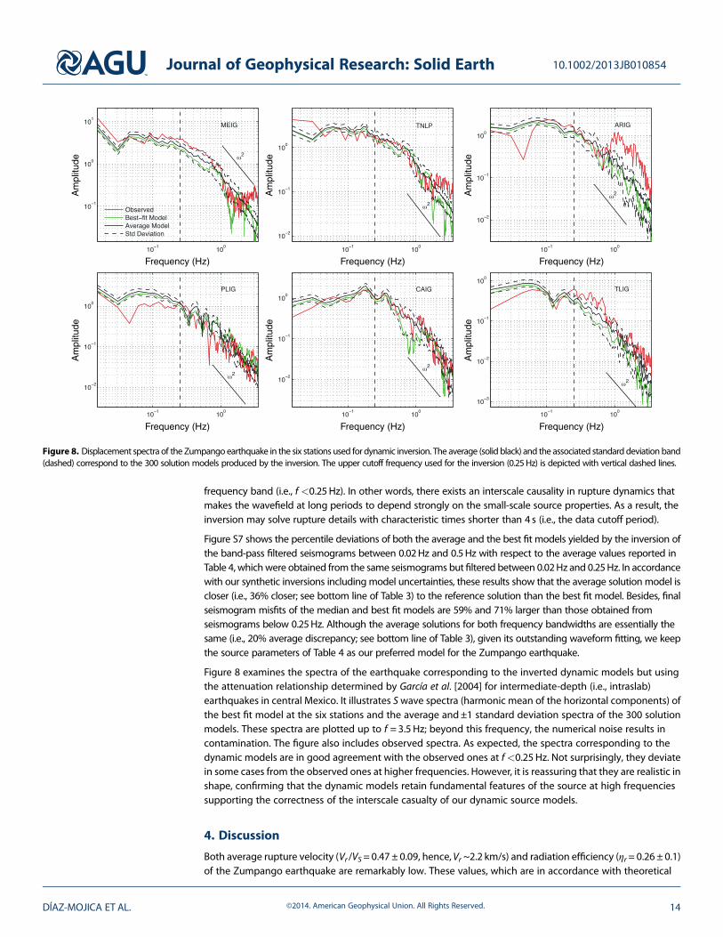
Figure 8 examines the spectra of the earthquake corresponding to the inverted dynamic models but usingthe attenuation relationship determined by García et al. [2004] for intermediate-depth (i.e., intraslab)earthquakes in central Mexico. It illustrates Swave spectra (harmonic mean of the horizontal components) ofthe best fit model at the six stations and the average and±1 standard deviation spectra of the 300 solutionmodels. These spectra are plotted up to f =3.5 Hz; beyond this frequency, the numerical noise results incontamination. The figure also includes observed spectra. As expected, the spectra corresponding to thedynamic models are in good agreement with the observed ones at f <0.25 Hz. Not surprisingly, they deviatein some cases from the observed ones at higher frequencies. However, it is reassuring that they are realistic inshape, confirming that the dynamic models retain fundamental features of the source at high frequenciessupporting the correctness of the interscale casualty of our dynamic source models.

4. Discussion

Both average rupture velocity (Vr /VS=0.47 ± 0.09, hence,Vr ~2.2 km/s) and radiation efficiency (ηr= 0.26 ± 0.1)of the Zumpango earthquake are remarkably low. These values, which are in accordance with theoretical

Am

plitu

de

Frequency (Hz) Frequency (Hz) Frequency (Hz)

Frequency (Hz) Frequency (Hz) Frequency (Hz)

Am

plitu

de

Am

plitu

deA

mpl

itude

Am

plitu

deA

mpl

itude

Figure 8. Displacement spectra of the Zumpango earthquake in the six stations used for dynamic inversion. The average (solid black) and the associated standard deviation band(dashed) correspond to the 300 solution models produced by the inversion. The upper cutoff frequency used for the inversion (0.25Hz) is depicted with vertical dashed lines.



expectations for a Mode II dynamic crack propagation [Kanamori and Rivera, 2006], are typical of slow,interplate tsunami earthquakes [e.g., Kanamori and Kikuchi, 1993; Venkataraman and Kanamori, 2004].Tsunami earthquakes are characterized by large (Ms-Mw) disparity [Kanamori and Kikuchi, 1993] andanomalously low value of Er and the ratio Er/M0 [Newman and Okal, 1998; Ammon et al., 2006]. The radiatedenergy of the Zumpango event (Er= (5.4 ±3.1) × 1014 J) is close to those of other Mexican earthquakes of similarM0 irrespective of their faulting mechanism and depth (Pérez-Campos, personal communication, 2013). The sameis true with its ratio Er/M0=5.7 × 10� 5 in a large range of seismicmoments (even for the value of Er obtained fromteleseismic records by the NEIC which is 1 order of magnitude smaller; see last section and Figure 11 of UNAMSeismology Group [2013]). This observation is not surprising for normal-faulting earthquakes in the subductedCocos plate, which systematically produce high peak ground accelerations [García et al., 2005; Singh et al., 2013]. Itseems then to be a paradox that prevents conciliating two main observations: (1) a slow and inefficient ruptureprocess and (2) a remarkably high radiation of short period waves.

Low radiation efficiency and high Er imply very high fracture energy, G (equation (9)), which makes thisearthquake highly energetic. The available potential energy for the dynamic process of faulting is ΔW0 =(1.98 ± 0.66) × 1015 J (equations (7) and (9)), from which we deduce that 73% or more (i.e., 82% for the best fitmodel; see Table 4) was not radiated (i.e., it was dissipated as fracture energy) and must have been used topropagate the rupture. Most shallow crust and interplate earthquakes have radiation efficiencies larger than 0.5[Venkataraman and Kanamori, 2004], which implies G< Er. For the Zumpango event, ηr=0.26± 0.1 (andηr=0.18 for the best fit model) soG=2.7Er (andG=4.7Er for the best fit model). In a closer view, our estimate forthe specific fracture energy, Gc, or breakdown work density (Wb=G/A) as defined by Tinti et al. [2005] is close to1.7 × 107 J/m2 (Table 4), which is about 10 times larger than expected for shallow crust earthquakes based on aregression analysis by these authors. In contrast, as compared to other estimates for this kind of earthquakes byAbercrombie and Rice [2005] and Lancieri et al. [2012] using a different approach based on spectral analysisfor ω2 source models, although dispersion is high and the comparison is not obvious, the estimate for theZumpango earthquake is in general agreement. In our simple slip-weakening friction model, this largeamount of nonradiated energy is spent in mechanical work done by fault tractions during the stressbreakdown. However, the actual manner in which it is partitioned to produce plastic strain, off-fault fracturing,heat, or any other dissipative process, especially at intermediate depths, still is a matter of debate, althoughresent observations favor the thermal shear runaway (with possible partial melting) as the dominant physicalmechanism [Prieto et al., 2013]. What is true is that energy dissipation controls rupture speed. The higher thedissipation, the lower is Vr despite the high energy radiation observed for this earthquake.

The large stress drop determined for the Zumpango earthquake (Δτ =29.2 ± 6.2 MPa, Table 4), which is inaccordance with independent estimates for intraslab quakes in central Mexico [García et al., 2004], the observedlow rupture speed, and high-energy dissipation are thus logical and compatible. Considering a slip-weakening

distance of 0.7m (Table 4) and taking D ¼ 1:8 m=s as the mean slip rate during the initial dislocation phase(Figure 7), the stress breakdown should have taken place in about 0.4 s, which is a reasonable value even forcrustal earthquakes [Mikumo et al., 2003; Cruz-Atienza et al., 2009]. The peak slip rate (PSR) is approximatelyreached at the time when the stress drop is completed [Mikumo et al., 2003; Cruz-Atienza et al., 2009] so thatby taking 3.5m/s as the maximum PSR (Figure 7) the focal particles acceleration produced by the stressdrop should be close to 1 g (i.e., ~8.8m/s2) during the initiation and arrest of the rupture process.

Our source model is essentially a penny shape crack with radial rupture speed. For Sato and Hirasawa’s [1973]

source model, which satisfies the exact slip solution for a circular shear crack by Eshelby [1957], we haveΔτ ≈

7π=24ð Þ Vs=Vrð Þ μD=2Vs

� . Taking Vs/Vr=2.1 (Table 4), this model predicts Δτ ≈ 28.1 MPa, which is consistent

with our results. This is simply telling us that, given a slow rupture propagation process, to achieve accelerationsclose to 1 g in a deep focal region where the shear modulus is high, the stress drop must be several times (i.e.,about 4 times) higher than those of shallower interplate earthquakes [García et al., 2004]. This also explainsstrong high-frequency radiation (and therefore large Er) from intermediate-depth intraslab events despite theirslow and inefficient rupture process, as previously discussed and shown for the earthquake studied here.

Error analysis discussed in section 2.4 and the supporting information yields a set of solution modelssatisfying the same ground motion misfit criterion. Differences between these models (e.g., between the



average and the best fit models) may be significant. However, estimates of the nondimensional K parameter(equation (10)) (1.01 ± 0.22 and 0.84 for the best fit model, Table 4), which reveals the general dynamiccharacter of earthquakes, is constrained to a small region predicting subshear ruptures and perfectly inagreement with the range determined by Ruiz and Madariaga [2011, Figure 4] for their best solution modelsof the Mw6.7 intraslab Michilla earthquake. Our synthetic inversion tests also revealed that the averagesolution model is closer to the actual solution than the best fit model if uncertainty is present in the sourcelocation (Figure S5). The average model error for an epicentral mislocation of 8 km to the south, which is areasonable value given the number of local stations used to relocate the event, is ~30% smaller than that ofthe best fit solution (see Table 3). In contrast, both errors are similar and close to 15% (Figure S6) if the bulkproperties surrounding the source are 5% lower than the actual ones (see Table 3). Besides, the uncertaintyassociated to each parameter includes, in most of cases, the corresponding target value.

5. Conclusions

We have developed an inversion method for imaging the earthquakes source dynamics from regionalrecords of ground motions. The method is based in genetic algorithms and is able to simultaneously solvehundreds of computationally expensive forward problems via MPI, like the one required here for modelingthe spontaneous rupture process. The source model follows an elliptical patch approach where rupture isgoverned by constant parameters determining the static stress drop and the cohesive forces evolutionthrough a slip-weakening constitutive law. Our method allows estimation of errors in both inverted andderived source parameters. If a good knowledge of the source location and the velocity structure is available,then the rupture speed (Vr), the rupture area (A), and the stress drop (Δτ), which are difficult to resolve inkinematic source inversions, are well constrained and may have errors of ~30%, ~12%, and ~10%,respectively. In contrast, parameters like the radiated energy (Er), the radiation efficiency (ηr), and the fractureenergy (G) have larger errors, around ~70%, ~40%, and ~25%, respectively.

We applied the method to the Mw 6.5 intermediate depth (62 km) Zumpango earthquake and found twomain features of the source process: (1) rupture speed (Vr/VS= 0.47 ± 0.09, i.e., about 2.2 km/s) and radiationefficiency (ηr= 0.26 ± 0.1) were remarkably low and (2) energy radiation (Er= (0.54 ± 0.31) × 1015J and the ratioEr/M0 = 5.7 × 10� 5) is similar to typical values for Mexican thrust events. These observations imply both largeenergy dissipation (i.e., more than 73% of ΔW0, the available potential energy for the dynamic process offaulting) and large stress drop (Δτ = 29.2 ± 6.2 MPa) in the focal region. It is interesting to note that Zumpangoearthquake and the deep 1994 Bolivian earthquake (Mw8.3; depth = 637 km) [Kanamori et al., 1998] sharesome fundamental features (i.e., slow rupture speed, low radiation efficiency, high stress drop, and smallrupture area), as it also does the intermediate-depth seismicity of the Bucaramanga nest for the stress dropand the radiation efficiency [Prieto et al., 2013].

ReferencesAmmon, C. J., H. Kanamori, T. Lay, and A. A. Velasco (2006), The 17 July 2006 Java tsunami earthquake (Mw7.8), Geophys. Res. Lett., 33, L24308,

doi:10.1029/2006GLO26303.Andrews, D. J. (1976), Rupture velocity of plane strain shear cracks, J. Geophys. Res., 81, 5679–5687, doi:10.1029/JB081i032p05679.Abercrombie, R. E., and J. R. Rice (2005), Can observations of earthquake scaling constrain slip weakening?, Geophys. J. Int., 162(2), 406–424,

doi:10.1111/j.1365-246X.2005.02579.x.Bizzarri, A., and M. Cocco (2003), Slip-weakening behavior during the propagation of dynamic ruptures obeying rate- and state dependent

friction laws, J. Geophys. Res., 108(B8), 2373, doi:10.1029/2002JB002198.Bouchon, M. (1981), A simple method to calculate Green’s Functions for elastic layered media, Bull. Seismol. Soc. Am., 71, 959–971.Brocher, T. M. (2008), Key elements of regional seismic velocity models for long period ground motion simulations, J. Seismol., 12, 217–221,

doi:10.1007/s10950-007-9061-3.Burridge, R., G. Kohn, and L. B. Freund (1979), The stability of rapid mode II shear crack with finite cohesive friction, J. Geophys. Res., 85,

2210–2222, doi:10.1029/JB084iB05p02210.Campillo, M., S. K. Singh, N. Shapiro, J. Pacheco, and R. B. Herrmann (1996), Crustal structure south of the Mexican volcanic belt, based on

group velocity dispersion, Geofis. Int., 35, 361–370.Corish, S. C., R. Bradley, and K. B. Olsen (2007), Assessment of a nonlinear dynamic rupture inversion technique, Bull. Seismol. Soc. Am., 97(3),

901–914, doi:10.1785/0120060066.Coutant, O. (1989), Program of numerical simulation AXITRA [in French], Res. Rep. LGIT, Univ. Joseph Fourier, Grenoble, France.Cruz-Atienza, V. M., and J. Virieux (2004), Dynamic rupture simulation of non-planar faults with a finite-difference approach, Geophys. J. Int.,

158, 939–954.Cruz-Atienza V. M., and K. B. Olsen (2010), Supershear mach-waves expose the fault breakdown slip, in Earthquake With Supershear Rupture

Speeds, edited by S. Das and M. Bouchon, Tectonophysics, 493, 285–296, doi:10.1016/j.tecto.2010.05.012.Cruz-Atienza, V. M., J. Virieux, and H. Aochi (2007), 3D finite-difference dynamic-rupture modelling along non-planar faults, Geophysics, 72,

SM123, doi:10.1190/1.2766756.



AcknowledgmentsWe thank Hiroo Kanamori, Steven Day,Jean Virieux, Sergio Ruiz, and VíctorHugo Espíndola for fruitful discussions.The data for this paper are availableupon proper request at the ServicioSismológico Nacional (SSN) and theInstituto de Ingeniería, both at UNAM.This work was possible, thanks to theUNAM-PAPIIT grants IN119409,IN113814, and IN111314, the Mexican“Consejo Nacional de Ciencia yTecnología” (CONACyT) under grant80205, and the French “AgenceNationale de la Recherche” under grantANR-2011-BS56-017.

http://dx.doi.org/10.1029/2006GLO26303

http://dx.doi.org/10.1029/JB081i032p05679

http://dx.doi.org/10.1111/j.1365-246X.2005.02579.x

http://dx.doi.org/10.1029/2002JB002198

http://dx.doi.org/10.1007/s10950-007-9061-3

http://dx.doi.org/10.1029/JB084iB05p02210

http://dx.doi.org/10.1785/0120060066

http://dx.doi.org/10.1016/j.tecto.2010.05.012

http://dx.doi.org/10.1190/1.2766756

Cruz-Atienza, V. M., K. B. Olsen, and L. A. Dalguer (2009), Estimation of the breakdown slip from strong-motion seismograms: Insights fromnumerical experiments, Bull. Seismol. Soc. Am., 99, 3454–3469, doi:10.1785/0120080330.

Cruz-Atienza, V. M., A. Iglesias, J. F. Pacheco, N. M. Shapiro, and S. K. Singh (2010), Crustal structure below the Valley of Mexico estimated fromreceiver functions, Bull. Seismol. Soc. Am., 100, 3304–3311, doi:10.1785/0120100051.

Dalguer, L. A., and S. Day (2007), Staggered-grid split-node method for spontaneous rupture simulation, J. Geophys. Res., 112, B02302,doi:10.1029/2006JB004467.

Das, S., and K. Aki (1977), Fault plane with barriers: A versatile earthquake model, J. Geophys. Res., 82, 5658–5670, doi:10.1029/JB082i036p05658.

Das, S., and B. K. Kostrov (1990), Inversion for seismic slip rate history and distribution with stabilizing constraints: Application to the 1986Andreanof Islands Earthquake, J. Geophys. Res., 95(B5), 6899–6913, doi:10.1029/JB095iB05p06899.

Day, S. M. (1982), Three-dimensional simulation of spontaneous rupture: The effect of nonuniform prestress, Bull. Seismol. Soc. Am., 72, 1881–1902.Díaz-Mojica, J. (2012), Inversión de la dinámica de sismos mexicanos, McS thesis, Posgrado en Ciencias de la Tierra, Universidad Nacional

Autónoma de México, Mexico City, Mexico.Di Carli, S., C. Francois-Holden, S. Peyrat, and R. Madariaga (2010), Dynamic inversion of the 2000 Tottori earthquake based on elliptical

subfault approximations, J. Geophys. Res., 115, B12328, doi:10.1029/2009JB006358.Eshelby, J. D. (1957), The determination of the elastic field of an ellipsoidal inclusion and related problems, Proc. R. Soc. London, Ser. A, 241,

376–396.Fernández de Vega, F., and E. Cantú-Paz (2010), Parallel and Distributed Computational Intelligence, Studies in Comput. Intell., vol. 269, Springer,

Berlin, doi:10.1007/978-3-642-10675-0.Freund, L. B. (1989), Dynamic Fracture Mechanics, Cambridge Univ. Press, Cambridge, U. K.García, D., S. K. Singh, M. Herraíz, J. F. Pacheco, and M. Ordaz (2004), Inslab earthquakes of central Mexico: Q, source spectra and stress drop,

Bull. Seismol. Soc. Am., 94, 789–802.García, D., S. K. Singh, M. Herráiz, M. Ordaz, and J. F. Pacheco (2005), Inslab earthquakes of central Mexico: Peak ground-motion parameters

and response spectra, Bull. Seismol. Soc. Am., 95, 2272–2282.Goldberg, D. E. (1989), Genetic Algorithms in Search, Optimization and Machine Learning, pp. 432, Addison Wesley, Reading, Mass.Guatteri, M., and P. Spudich (2000), What can strong motion data tell us about slip weakening fault friction laws?, Bull. Seismol. Soc. Am., 90,

98–116.Holland, J. H. (1975), Adaptation in Natural and Artificial Systems, pp. 228, Univ. Mich. Press, Ann Arbor.Husseini, M. I. (1977), Energy balance for motion along a fault, Geophys. J. R. Astron. Soc., 49, 699–714.Ida, Y. (1972), Cohesive force across tip of a longitudinal-shear crack Griffith specific surface energy, J. Geophys. Res., 77, 3796–3805,

doi:10.1029/JB077i020p03796.Ide, S., and M. Takeo (1997), Determination of constitutive relations of fault slip based on seismic wave analysis, J. Geophys. Res., 102,

27,379–27,391, doi:10.1029/97JB02675.Iglesias, A., V. M. Cruz-Atienza, N. M. Shapiro, S. K. Singh, and J. F. Pacheco (2001), Crustal structure of south-central Mexico estimated from

the inversion of surface waves dispersion curves using genetic and simulated annealing algorithms, Geofis. Int., 40, 181–190.Kanamori, H., and E. E. Brodsky (2004), The physics of earthquakes, Rep. Prog. Phys., 67, 1429–1496.Kanamori, H., and L. Rivera (2006), Energy partitioning during an earthquake, in Earthquakes: Radiated Energy and the Physics of Faulting,

Geophys. Monogr. Ser., vol. 170, edited by R. Abercrombie et al., pp. 3–13, AGU, Washington, D. C., doi:10.1029/170GM03.Kanamori, H., J. Mori, E. Hauksson, T. H. Heaton, L. K. Hutton, and L. M. Jones (1993), Determination of earthquake energy release and ML

using terrascope, Bull. Seismol. Soc. Am., 83, 330–346.Kanamori, H., D. L. Anderson, and T. H. Heaton (1998), Frictional melting during the rupture of the 1994 Bolivian earthquake, Science, 279,

839–842.Kim, Y., R. W. Clayton, and J. M. Jackson (2010), Geometry and seismic properties of the subducting Cocos plate in central Mexico, J. Geophys.

Res., 115, B06310, doi:10.1029/2009JB006942.Kostrov, B. V. (1966), Unsteady propagation of longitudinal cracks, J. Appl. Math. Mech., 30, 1241–1248.Kostrov, B. V., (1974), Seismic moment and energy of earthquakes, and seismic flow of rock [Engl. transl.], Izv. Earth Phys., 1, 23–40.Lancieri, M., R. Madariaga, and F. Bonilla (2012), Spectral scaling of the aftershocks of the Tocopilla 2007 earthquake in northern Chile,

Geophys. J. Int., doi:10.1111/j.1365-246X.2011.05327.x.Lemoine, A., R. Madariaga, and J. Campos (2002), Slab-pull and slab-push earthquakes in the Mexican, Chilean and Peruvian subduction

zones, Phys. Earth Planet. Inter., 132(1–3), 157–175.Madariaga, R. (1976), Dynamics of an expanding circular fault, Bull. Seismol. Soc. Am., 66, 639–666.Madariaga, R., and K. B. Olsen (2000), Criticality of rupture dynamics in 3-D, Pure Appl. Geophys., 157, 1981–2001.Madariaga, R., K. B. Olsen, and R. J. Archuleta (1998), Modeling dynamic rupture in a 3D earthquake fault model, Bull. Seismol. Soc. Am., 88,

1182–1197.Marcinkovich, C., and K. Olsen (2003), On the implementation of perfectly matched layers in a three-dimensional fourth-order velocity-stress

finite difference scheme, J. Geophys. Res., 108(B5), 2276, doi:10.1029/2002JB002235.Menke, W. (2012), Geophysical Data Analysis: Discrete Inverse Theory, 3rd ed. (textbook), 293 pp., Academic Press (Elsevier), Oxford, U. K.,

doi:10.1016/B978-0-12-397160-9.00001-1.Mikumo, T., and T. Miyatake (1978), Dynamical rupture process on a three-dimensional fault with non-uniform frictions and near field seismic

waves, Geophys. J. R. Astron. Soc., 54, 417–438.Mikumo, T., and T. Miyatake (1993), Dynamic rupture processes on a dipping fault, and estimate of stress drop and strength excess from the

results of waveform inversion, Geophys. J. Int., 112, 481–496.Mikumo, T., K. B. Olsen, E. Fukuyama, and Y. Yagi (2003), Stress-breakdown time and slip-weakening distance inferred from slip-velocity

functions on earthquake faults, Bull. Seismol. Soc. Am., 93(1), 264–282.Newman, A. V., and E. A. Okal (1998), Teleseismic estimates of radiated seismic energy: The E/M0 discriminant for tsunami earthquakes,

J. Geophys. Res., 103(26), 885–898.Olsen, K. B., et al. (2009), ShakeOut-D: Ground motion estimates using an ensemble of large earthquakes on the southern San Andreas Fault

with spontaneous rupture propagation, Geophys. Res. Lett., 36, L04303, doi:10.1029/2008GL036832.Pacheco, J. F., and S. K. Singh (2010), Seismicity and state of stress in Guerrero segment of the Mexican subduction zone, J. Geophys. Res., 115,

B01303, doi:10.1029/2009JB006453.Palmer, A., and J. R. Rice (1973), The grow of slip surfaces in the progressive failure of overconsolidated clay, Proc. R. Soc. London, Ser. A, 332,

527–548.



http://dx.doi.org/10.1785/0120080330

http://dx.doi.org/10.1785/0120100051

http://dx.doi.org/10.1029/2006JB004467



http://dx.doi.org/10.1029/JB095iB05p06899

http://dx.doi.org/10.1029/2009JB006358

http://dx.doi.org/10.1007/978-3-642-10675-0


http://dx.doi.org/10.1029/97JB02675

http://dx.doi.org/10.1029/170GM03

http://dx.doi.org/10.1029/2009JB006942


http://dx.doi.org/10.1029/2002JB002235

http://dx.doi.org/10.1016/B978-0-12-397160-9.00001-1

http://dx.doi.org/10.1029/2008GL036832

http://dx.doi.org/10.1029/2009JB006453

Pérez-Campos, X., Y. Kim, A. Husker, P. M. Davis, R. W. Clayton, A. Iglesias, J. F. Pacheco, S. K. Singh, V. C. Manea, and M. Gurnis (2008), Horizontalsubduction and truncation of the Cocos Plate beneath central Mexico, Geophys. Res. Lett., 35, L18303, doi:10.1029/2008GL035127.

Pérez-Campos, X., S. K. Singh, and G. C. Beroza (2003), Reconciling teleseismic and regional estimates of seismic energy, Bull. Seismol. Soc.Am., 93(5), 2123–2130.

Peyrat, S., and K. B. Olsen (2004), Nonlinear dynamic rupture inversion of the 2000 Western Tottori, Japan, earthquake, Geophys. Res. Lett., 31,L05604, doi:10.1029/2003GL019058.

Peyrat, S., and P. Favreau (2010), Kinematic and spontaneous rupture models of the 2005 Tarapacá intermediate depth, Geophys. J. Int., 181,369–381.

Pikaia (2002), Sofware developed by P. Charbonneau and B. Knapp. [Available at www.whitedwarf.org/parallel.]Prieto, G. A., M. Florez, S. A. Barrett, and G. C. Beroza (2013), Seismic evidence for thermal runaway during intermediate-depth earthquake

rupture, Geophys. Res. Lett., 40, 1–5, doi:10.1002/2013GL058109.Rivera, L., and H. Kanamori (2005), Representations of the radiated energy in earthquakes, Geophys. J. Int., 162(1), 148–155, doi:10.1111/

j.1365-246X.2005.02648.x.Ruiz, S., and R. Madariaga (2011), Determination of the friction law parameters of the Mw 6.7 Michilla earthquake in northern Chile by

dynamic inversion, Geophys. Res. Lett., 38, L09317, doi:10.1029/2011GL047147.Ruiz, S., and R. Madariaga (2013), Kinematic and dynamic inversion of the 2008 Northern Iwate earthquake, Bull. Seismol. Soc. Am., 103,

694–708.Sato, T., and T. Hirasawa (1973), Body wave spectra from propagating shear waves, J. Phys. Earth, 21, 415–431.Singh, S. K., and M. Pardo (1993), Geometry of the Benioff Zone and state of stress in the overriding plate in Central Mexico, Geophys. Res.

Lett., 20, 1483–1486, doi:10.1029/93GL01310.Singh, S. K., and M. Ordaz (1994), Seismic energy release in Mexican subduction zone earthquakes, Bull. Seismol. Soc. Am., 84, 1533–1550.Singh, S. K., J. F. Pacheco, B. K. Bansal, X. Pérez-Campos, R. S. Dattatrayam, and G. Suresh (2004), A source study of the Bhuj, India, earthquake

of 26 January 2001 (Mw 7.6), Bull. Seismol. Soc. Am., 94(4), 1195–1206.Singh, S. K., M. Ordaz, X. Pérez-Campos, and A. Iglesias (2013), Intraslab versus interplate earthquakes as recorded in Mexico City: Implications

for seismic hazard, Earthquake Spectra, doi:10.1193/110612EQS324M.Song, T.-R. A., D. V. Helmberger, M. R. Brudzinski, R. W. Clayton, P. Davis, X. Pérez-Campos, and S. K. Singh (2009), Subducting slab ultra-slow

velocity layer coincident with silent earthquake in southern Mexico, Science, 324, 502–506, doi:10.1126/science.1167595.Spudich, P., and M. Guatteri (2004), The effect of bandwidth limitations on the inference of earthquake slip-weakening distance from seis-

mograms, Bull. Seismol. Soc. Am., 94, 2028–2036.Spudich, P., and D. P. Miller (1990), Seismic site effects and the spatial interpolation of earthquake seismograms: Results using aftershocks of

the 1986 North Palm Springs, California, earthquake, Bull. Seismol. Soc. Am., 80, 1504–1532.Suárez, G., T. Monfret, G. Wittlinger, and C. David (1990), Geometry of subduction and depth of the seismogenic zone in the Guerrero gap,

Mexico, Nature, 345, 336–338.Tago, J., V. M. Cruz-Atienza, J. Virieux, V. Etienne, and F. J. Sánchez-Sesma (2012), A 3D hp-adaptive discontinuous Galerkin method for

modeling earthquake dynamics, J. Geophys. Res., 117, B09312, doi:10.1029/2012JB009313.Tinti, E., P. Spudich, and M. Cocco (2005), Earthquake fracture energy inferred from kinematic rupture models on extended faults, J. Geophys.

Res., 110, B12303, doi:10.1029/2005JB003644.UNAM Seismology Group (2013), Ometepec-Pinotepa Nacional, Mexico Earthquake of 20 March 2012 (Mw7.5): A preliminary report, Geofis.

Int., 52(2), 173–196.Vallée, M., and M. Bouchon (2004), Imaging coseismic rupture in far field by slip patches, Geophys. J. Int., 156, 615–630.Venkataraman, A., and H. Kanamori (2004), Observational constraints on the fracture energy of subduction zone earthquakes, J. Geophys.

Res., 109, B05302, doi:10.1029/2003JB002549.Virieux, J., and R. Madariaga (1982), Dynamic faulting studied by a finite difference method, Bull. Seismol. Soc. Am., 72, 345–369.



http://dx.doi.org/10.1029/2008GL035127

http://dx.doi.org/10.1029/2003GL019058

http://www.whitedwarf.org/parallel

http://dx.doi.org/10.1002/2013GL058109



http://dx.doi.org/10.1029/2011GL047147

http://dx.doi.org/10.1029/93GL01310

http://dx.doi.org/10.1193/110612EQS324M

http://dx.doi.org/10.1126/science.1167595

http://dx.doi.org/10.1029/2012JB009313

http://dx.doi.org/10.1029/2005JB003644

http://dx.doi.org/10.1029/2003JB002549

dynamic source inversion of the m6.5 intermediate-depth...

Documents