dynamic programming & optimal control advanced … · 2020-04-03 · dynamic programming &...
TRANSCRIPT

Dynamic Programming & Optimal ControlAdvanced Macroeconomics
Ph.D. Program in Economics, HUST
Changsheng Xu, Shihui Ma, Ming Yi ([email protected])
School of Economics, Huazhong University of Science and Technology
This version: November 21, 2019
Ming Yi (Econ@HUST) Doctoral Macroeconomics Notes on D.P. & O.C. 1 / 61

Course information:http://www.yiming.website/teaching/2019fdmacro/
This lecture note is based mainly on selected materials in Chapter 6and Chapter 7 of Acemoglu (2008).
Ming Yi (Econ@HUST) Doctoral Macroeconomics Notes on D.P. & O.C. 2 / 61

(a) Richard E. Bellman (1920-1984) (b) Lev S. Pontryagin (1908-1988)
Figure 1: Pictures of the two pioneers.
Ming Yi (Econ@HUST) Doctoral Macroeconomics Notes on D.P. & O.C. 3 / 61

Dynamic Programming:the Problems Canonical Form
Canonical Discrete-Time Infinite-Horizon OptimizationProblemCanonical form of the problem:
sup{x(t),y(t)}∞t=0
∞∑t=0
βtU(t, x(t), y(t)) (1)
subject to y(t) ∈ G(t, x(t)) for all t ≥ 0, (2)x(t + 1) = f(t, x(t), y(t)) for all t ≥ 0, (3)x(0) given. (4)
“sup” interchangeable with “max” within the note. β ∈ [0, 1).x(t) ∈ X ⊂ RKx : state variables (state vector), y(t) ∈ Y ⊂ RKy :control variables (control vector). Kx,Ky ≥ 1.instantaneous payoff function U : Z+ × X × Y → R. Objectivefunction:
∑∞t=0 β
tU(t, x(t), y(t)). Correspondence G : Z+ × x ⇒ Y.Ming Yi (Econ@HUST) Doctoral Macroeconomics Notes on D.P. & O.C. 4 / 61

Dynamic Programming:the Problems Problem A2
Problem A1
The canonical form is rewritten as Problem A1:
V∗(0, x(0)) = sup{x(t)}∞t=0
∞∑t=0
βtU(t, x(t), x(t + 1)) (5)
subject to x(t + 1) ∈ G(t, x(t)) for all t ≥ 0, (6)x(0) given. (7)
Problem A1 is identical to the canonical problem above.New expression, why bother?V∗(0, x(0)) obtained upon optimal plan {x∗(t + 1)}∞t=0 ∈ X∞.What if symbol ∞ is replaced by some T ∈ Z+?Based on G, U, f, the definitions of G, U, and V∗ are trivial.
Ming Yi (Econ@HUST) Doctoral Macroeconomics Notes on D.P. & O.C. 5 / 61

Dynamic Programming:the Problems Problem A2
Problem A1 (Continued)
Problem A1:
V∗(0, x(0)) = sup{x(t)}∞t=0
∞∑t=0
βtU(t, x(t), x(t + 1))
subject to x(t + 1) ∈ G(t, x(t)) for all t ≥ 0,
x(0) given.
Try to define G(t, x(t)).
G(t, x(t)) = {f(t, x(t), y(t)) ∈ X | yt ∈ G(t, x(t))}
Ming Yi (Econ@HUST) Doctoral Macroeconomics Notes on D.P. & O.C. 6 / 61

Dynamic Programming:the Problems Problem A2
Problem A2
In this note, we focus only on Problem A2:
V∗(x(0)) = sup{x(t)}∞t=0
∞∑t=0
βtU(x(t), x(t + 1)) (8)
subject to x(t + 1) ∈ G(x(t)) for all t ≥ 0, (9)x(0) given. (10)
Problem A2 is a stationary form of Problem A1: U and G do notexplicitly depend on time.Stationary dynamic programming.Applicable to most economic applications.
Ming Yi (Econ@HUST) Doctoral Macroeconomics Notes on D.P. & O.C. 7 / 61

Bellman Equation Problem A3
Problem A3
Let us consider Problem A3:
V(x) = supy∈G(x)
{U(x, y) + βV(y)}, for all x ∈ X. (11)
The recursively defined V(x) is called Bellman Equation.The previous problem of finding a sequence {x∗(t + 1)}∞t=0 isreplaced by the problem of finding a function V(x).V(·) is called value function.Define policy function π(·) by y∗ = π(x).So V(x) = U(x, π(x)) + βV(π(x)).Once the value function is known, it is straightforward to inducethe policy function.
Ming Yi (Econ@HUST) Doctoral Macroeconomics Notes on D.P. & O.C. 8 / 61

Bellman Equation Problem A3
An Example
The problem is given in the canonical form:
max{k(t),c(t)}∞t=0
∞∑t=0
βtu(c(t)),
subject to k(t + 1) = f(k(t)) + (1− δ)k(t)− c(t),
where k(t) ≥ 0 and given k(0) > 0, u : R+ → R.
Try to transform the canonical problem above to Problem A2 and A3.
Ming Yi (Econ@HUST) Doctoral Macroeconomics Notes on D.P. & O.C. 9 / 61

Bellman Equation Problem A3
V∗ satisfies Bellman EquationRecalling the relationship between V∗(x(0)) and {x∗(t + 1)}∞t=1 inProblem A2:
V∗(x(0)) =∞∑
t=0
βtU(x∗(t), x∗(t + 1)) (12)
= U(x(0), x∗(1)) + β
∞∑s=0
βsU(x∗(s + 1), x∗(s + 2)) (13)
= U(x(0), x∗(1)) + βV∗(x∗(1)) (14)= sup
y∈G(x(0)){U(x(0), y) + βV∗(y)}, ∀x(0) ∈ X. (15)
Equation (14): An optimal plan from t = 0 must also be anoptimal plan from t = 1.Equation (15): An optimal plan solves the optimization problem.x∗(t + 1) = π(x∗(t)) holds for all t.
Ming Yi (Econ@HUST) Doctoral Macroeconomics Notes on D.P. & O.C. 10 / 61

Bellman Equation Problem A3
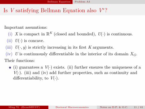
Is V satisfying Bellman Equation also V∗?
Important assumtions:(i) X is compact in RK (closed and bounded), U(·) is continuous.(ii) U(·) is concave.(iii) U(·, y) is strictly increasing in its first K arguments.(iv) U is continuously differentiable in the interior of its domain XG.Their functions:
(i) guarantees a V(·) exists. (ii) further ensures the uniqueness of aV(·). (iii) and (iv) add further properties, such as continuity anddifferentiability, to V(·).So, given the uniqueness, we know that V(·) satisfying is also V∗
solving Problem A2.
Ming Yi (Econ@HUST) Doctoral Macroeconomics Notes on D.P. & O.C. 11 / 61
Bellman Equation Problem A3
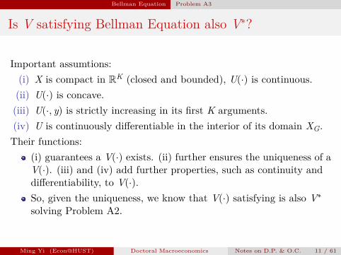
Is V satisfying Bellman Equation also V∗?
Important assumtions:(i) X is compact in RK (closed and bounded), U(·) is continuous.(ii) U(·) is concave.(iii) U(·, y) is strictly increasing in its first K arguments.(iv) U is continuously differentiable in the interior of its domain XG.Their functions:
(i) guarantees a V(·) exists. (ii) further ensures the uniqueness of aV(·). (iii) and (iv) add further properties, such as continuity anddifferentiability, to V(·).
So, given the uniqueness, we know that V(·) satisfying is also V∗
solving Problem A2.
Ming Yi (Econ@HUST) Doctoral Macroeconomics Notes on D.P. & O.C. 11 / 61
Bellman Equation Problem A3
Is V satisfying Bellman Equation also V∗?
Important assumtions:(i) X is compact in RK (closed and bounded), U(·) is continuous.(ii) U(·) is concave.(iii) U(·, y) is strictly increasing in its first K arguments.(iv) U is continuously differentiable in the interior of its domain XG.Their functions:
(i) guarantees a V(·) exists. (ii) further ensures the uniqueness of aV(·). (iii) and (iv) add further properties, such as continuity anddifferentiability, to V(·).So, given the uniqueness, we know that V(·) satisfying is also V∗
solving Problem A2.
Ming Yi (Econ@HUST) Doctoral Macroeconomics Notes on D.P. & O.C. 11 / 61
Bellman Equation Problem A3
Bellman Equation
We have shown that, under pretty weak assumptions, finding theV∗(·) in Problem A2 is equivalent to finding the V(·) in ProblemA3.We haven’t answer the question: Is it easier or more convenient tosearch for V(·) instead of V∗(·)?
To answer the question above, as well as to unfold the beauty ofthe Bellman Equation, we should take a detour by spending some(rewarding) time on contraction mapping.
Ming Yi (Econ@HUST) Doctoral Macroeconomics Notes on D.P. & O.C. 12 / 61

Bellman Equation Problem A3
Bellman Equation
We have shown that, under pretty weak assumptions, finding theV∗(·) in Problem A2 is equivalent to finding the V(·) in ProblemA3.We haven’t answer the question: Is it easier or more convenient tosearch for V(·) instead of V∗(·)?To answer the question above, as well as to unfold the beauty ofthe Bellman Equation, we should take a detour by spending some(rewarding) time on contraction mapping.
Ming Yi (Econ@HUST) Doctoral Macroeconomics Notes on D.P. & O.C. 12 / 61

Bellman Equation Contraction Mapping
Newton’s Method: A Taste
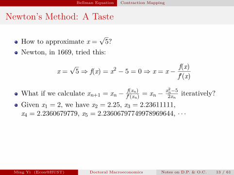
How to approximate x =√5?
Newton, in 1669, tried this:
x =√5 ⇒ f(x) = x2 − 5 = 0 ⇒ x = x − f(x)
f′(x)
What if we calculate xn+1 = xn − f(xn)f′(xn)
= xn − x2n−52xn
iteratively?Given x1 = 2, we have x2 = 2.25, x3 = 2.23611111,x4 = 2.2360679779, x5 = 2.23606797749978969644, · · ·this method is obviously applicable to many equation-solvingscenarios.We will show that the method here is a contraction mapping on aproperly defined domain.
Ming Yi (Econ@HUST) Doctoral Macroeconomics Notes on D.P. & O.C. 13 / 61

Bellman Equation Contraction Mapping
Newton’s Method: A Taste
How to approximate x =√5?
Newton, in 1669, tried this:
x =√5 ⇒ f(x) = x2 − 5 = 0 ⇒ x = x − f(x)
f′(x)
What if we calculate xn+1 = xn − f(xn)f′(xn)
= xn − x2n−52xn
iteratively?
Given x1 = 2, we have x2 = 2.25, x3 = 2.23611111,x4 = 2.2360679779, x5 = 2.23606797749978969644, · · ·this method is obviously applicable to many equation-solvingscenarios.We will show that the method here is a contraction mapping on aproperly defined domain.
Ming Yi (Econ@HUST) Doctoral Macroeconomics Notes on D.P. & O.C. 13 / 61
Bellman Equation Contraction Mapping
Newton’s Method: A Taste
How to approximate x =√5?
Newton, in 1669, tried this:
x =√5 ⇒ f(x) = x2 − 5 = 0 ⇒ x = x − f(x)
f′(x)
What if we calculate xn+1 = xn − f(xn)f′(xn)
= xn − x2n−52xn
iteratively?Given x1 = 2, we have x2 = 2.25, x3 = 2.23611111,x4 = 2.2360679779, x5 = 2.23606797749978969644, · · ·
this method is obviously applicable to many equation-solvingscenarios.We will show that the method here is a contraction mapping on aproperly defined domain.
Ming Yi (Econ@HUST) Doctoral Macroeconomics Notes on D.P. & O.C. 13 / 61

Bellman Equation Contraction Mapping
Newton’s Method: A Taste
How to approximate x =√5?
Newton, in 1669, tried this:
x =√5 ⇒ f(x) = x2 − 5 = 0 ⇒ x = x − f(x)
f′(x)
What if we calculate xn+1 = xn − f(xn)f′(xn)
= xn − x2n−52xn
iteratively?Given x1 = 2, we have x2 = 2.25, x3 = 2.23611111,x4 = 2.2360679779, x5 = 2.23606797749978969644, · · ·this method is obviously applicable to many equation-solvingscenarios.
We will show that the method here is a contraction mapping on aproperly defined domain.
Ming Yi (Econ@HUST) Doctoral Macroeconomics Notes on D.P. & O.C. 13 / 61

Bellman Equation Contraction Mapping
Newton’s Method: A Taste
How to approximate x =√5?
Newton, in 1669, tried this:
x =√5 ⇒ f(x) = x2 − 5 = 0 ⇒ x = x − f(x)
f′(x)
What if we calculate xn+1 = xn − f(xn)f′(xn)
= xn − x2n−52xn
iteratively?Given x1 = 2, we have x2 = 2.25, x3 = 2.23611111,x4 = 2.2360679779, x5 = 2.23606797749978969644, · · ·this method is obviously applicable to many equation-solvingscenarios.We will show that the method here is a contraction mapping on aproperly defined domain.
Ming Yi (Econ@HUST) Doctoral Macroeconomics Notes on D.P. & O.C. 13 / 61

Bellman Equation Contraction Mapping
Contraction Mapping
Definition 1Let (S, d) be a metric space and T : S → S be an operator mapping Sinto itself. If for some β ∈ (0, 1),
d(Tz1,Tz2) ≤ βd(z1, z2) for all z1, z2 ∈ S,
Then T is a contraction mapping (with modulus β).
A contraction mapping makes any couple of elements closer.
Ming Yi (Econ@HUST) Doctoral Macroeconomics Notes on D.P. & O.C. 14 / 61

Bellman Equation Contraction Mapping
Contraction Mapping (Continued)
Theorem 1(Contraction Mapping Theorem) Let (S, d) be a complete metric spaceand suppose that T : S → S is a contraction mapping. Then T has aunique z ∈ S such that
Tz = z.
Ming Yi (Econ@HUST) Doctoral Macroeconomics Notes on D.P. & O.C. 15 / 61

Bellman Equation Contraction Mapping
Contraction Mapping (Continued)
The formal proof of Theorem 1 is omitted here. The intuition,however, is quite straightforward: Starting from any given point inS, impose T infinitely many times. As the contraction mappingmakes the adjacent pair of points closer and closer, the resultingCauchy sequence must converges to a point in a complete space.
Don’t worry about the requirement “complete”. The spacesusually dealt with in Economics are all complete: the Euclideanspace, the space of continuous real-valued function on a compactset, and so on.
Ming Yi (Econ@HUST) Doctoral Macroeconomics Notes on D.P. & O.C. 16 / 61

Bellman Equation Contraction Mapping
Contraction Mapping (Continued)
The formal proof of Theorem 1 is omitted here. The intuition,however, is quite straightforward: Starting from any given point inS, impose T infinitely many times. As the contraction mappingmakes the adjacent pair of points closer and closer, the resultingCauchy sequence must converges to a point in a complete space.Don’t worry about the requirement “complete”. The spacesusually dealt with in Economics are all complete: the Euclideanspace, the space of continuous real-valued function on a compactset, and so on.
Ming Yi (Econ@HUST) Doctoral Macroeconomics Notes on D.P. & O.C. 16 / 61

Bellman Equation Contraction Mapping
Contraction Mapping (Continued)
Theorem 2(Applications of Contraction Mappings) Let (S, d) be a complete metricspace and T : S → S be a contraction mapping with Tz = z.(a) If S′ is a closed subset of S, and T(S′) ⊂ S′, then z ∈ S′.(b) Moreover, if T(S′) ⊂ S′′ ⊂ S′, then z ∈ S′′.
These results are irrelevant to the main materials in this note.Question: If you have the opportunity to draw a pretty precisemap of China and spread it out on the square in front of theschool building, are you capable of finding a point, if any, on themap, that coincides with its corresponding geographical locationon the earth?
Ming Yi (Econ@HUST) Doctoral Macroeconomics Notes on D.P. & O.C. 17 / 61

Bellman Equation Contraction Mapping
Contraction Mapping (Continued)
Theorem 2(Applications of Contraction Mappings) Let (S, d) be a complete metricspace and T : S → S be a contraction mapping with Tz = z.(a) If S′ is a closed subset of S, and T(S′) ⊂ S′, then z ∈ S′.(b) Moreover, if T(S′) ⊂ S′′ ⊂ S′, then z ∈ S′′.
These results are irrelevant to the main materials in this note.
Question: If you have the opportunity to draw a pretty precisemap of China and spread it out on the square in front of theschool building, are you capable of finding a point, if any, on themap, that coincides with its corresponding geographical locationon the earth?
Ming Yi (Econ@HUST) Doctoral Macroeconomics Notes on D.P. & O.C. 17 / 61

Bellman Equation Contraction Mapping
Contraction Mapping (Continued)
Theorem 2(Applications of Contraction Mappings) Let (S, d) be a complete metricspace and T : S → S be a contraction mapping with Tz = z.(a) If S′ is a closed subset of S, and T(S′) ⊂ S′, then z ∈ S′.(b) Moreover, if T(S′) ⊂ S′′ ⊂ S′, then z ∈ S′′.
These results are irrelevant to the main materials in this note.Question: If you have the opportunity to draw a pretty precisemap of China and spread it out on the square in front of theschool building, are you capable of finding a point, if any, on themap, that coincides with its corresponding geographical locationon the earth?
Ming Yi (Econ@HUST) Doctoral Macroeconomics Notes on D.P. & O.C. 17 / 61

Bellman Equation Contraction Mapping
Newton’s Method: Revisit
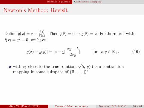
Define g(x) = x − f(x)f′(x) . Then f(x) = 0 → g(x) = x. Furthermore, with
f(x) = x2 − 5, we have
|g(x)− g(y)| = |x − y||xy − 5
2xy |, for x, y ∈ R+. (16)
with x1 close to the true solution,√5, g(·) is a contraction
mapping in some subspace of (R+, | · |)!The initialization point chosen in Newton’s method is crucial.
Ming Yi (Econ@HUST) Doctoral Macroeconomics Notes on D.P. & O.C. 18 / 61
Bellman Equation Contraction Mapping
Newton’s Method: Revisit
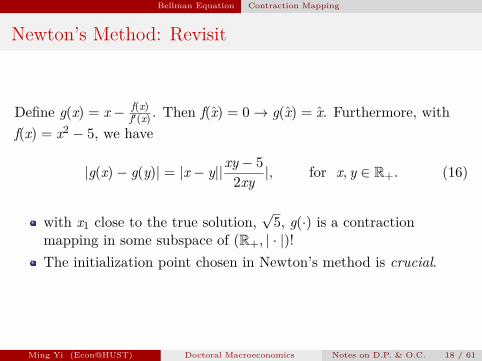
Define g(x) = x − f(x)f′(x) . Then f(x) = 0 → g(x) = x. Furthermore, with
f(x) = x2 − 5, we have
|g(x)− g(y)| = |x − y||xy − 5
2xy |, for x, y ∈ R+. (16)
with x1 close to the true solution,√5, g(·) is a contraction
mapping in some subspace of (R+, | · |)!
The initialization point chosen in Newton’s method is crucial.
Ming Yi (Econ@HUST) Doctoral Macroeconomics Notes on D.P. & O.C. 18 / 61
Bellman Equation Contraction Mapping
Newton’s Method: Revisit
Define g(x) = x − f(x)f′(x) . Then f(x) = 0 → g(x) = x. Furthermore, with
f(x) = x2 − 5, we have
|g(x)− g(y)| = |x − y||xy − 5
2xy |, for x, y ∈ R+. (16)
with x1 close to the true solution,√5, g(·) is a contraction
mapping in some subspace of (R+, | · |)!The initialization point chosen in Newton’s method is crucial.
Ming Yi (Econ@HUST) Doctoral Macroeconomics Notes on D.P. & O.C. 18 / 61

Bellman Equation Bellman Equation and Contraction Mapping
Bellman Equation and Contraction Mapping
Recall the Bellman equation:
V(x) = supy∈G(x)
{U(x, y) + βV(y)}, for all x ∈ X. (17)
= TV(x), for all x ∈ X, (18)
where the second equality is a definition of operator T.
We will show that T is a contraction mapping.Space for T to operate: all bounded functions defined on X.So T is a functional: It maps a function to another.How should we choose the metric, d(·), of the space?
Ming Yi (Econ@HUST) Doctoral Macroeconomics Notes on D.P. & O.C. 19 / 61

Bellman Equation Bellman Equation and Contraction Mapping
Define the Metric
For functions f, g defined on X, the supremum norm is used for metric:
d(f, g) = ∥f − g∥ = supx∈X
|f(x)− g(x)| (19)
The “distance” between two functions defined on X is determinedby the greatest “gap” between the two functions on X.You can, of course, adopt other kinds of metrics. But any welldefined norm will prove the same result as the supremum normdoes.
Ming Yi (Econ@HUST) Doctoral Macroeconomics Notes on D.P. & O.C. 20 / 61

Bellman Equation Bellman Equation and Contraction Mapping
Prove T is a Contraction Mapping
Proposition 1Let X ∈ RK and B(X) be the space of bounded functions f : X → Rdefined on X, equipped with the supremum norm ∥ · ∥, Define mappingT : B(X) → B(X) by
(Tf)(x) = supy∈G(x)
{U(x, y) + βf(y)}, ∀x ∈ X, ∀f ∈ B(X).
Then T is a contraction mapping.
Ming Yi (Econ@HUST) Doctoral Macroeconomics Notes on D.P. & O.C. 21 / 61

Bellman Equation Bellman Equation and Contraction Mapping
Prove T is a Contraction Mapping (Continued)Proof: Given f, g ∈ B(X),
f(x)− g(x) ≤ |f(x)− g(x)| ≤ ∥f − g∥ ∀x ∈ X (20)⇒ f(x) ≤g(x) + ∥f − g∥ ∀x ∈ X (21)⇒ (Tf)(x) = sup
y∈G(x){U(x, y) + βf(y)} ∀x ∈ X
≤ supy∈G(x)
{U(x, y) + βg(y) + β∥f − g∥} ∀x ∈ X
⇒ (Tf)(x) ≤ (Tg)(x) + β∥f − g∥ ∀x ∈ X (22)Analogously, (Tg)(x) ≤ (Tf)(x) + β∥f − g∥ ∀x ∈ X (23)
Combining (22) and (23) yields
∥Tf − Tg∥ = supx∈X
|(Tf)(x)− (Tg)(x)| ≤ β∥f − g∥ (24)
T is thus a contraction mapping.Ming Yi (Econ@HUST) Doctoral Macroeconomics Notes on D.P. & O.C. 22 / 61

Bellman Equation Bellman Equation and Contraction Mapping
V(x)
x
V∗ ≡ TV∗
V2
TV2
V1
TV1
Figure 2: T : B(X) → B(X) defined in the Bellman equation is a contraction mapping.
Ming Yi (Econ@HUST) Doctoral Macroeconomics Notes on D.P. & O.C. 23 / 61

Bellman Equation Bellman Equation and Contraction Mapping
Utilizing Contraction Mapping T
We have shown that T is a contraction mapping in space B(X).
So, T admits a unique fixed point, i.e., a unique V(·) such thatV ≡ TV.Recall that, the unique solution to the Bellman equation, V, isalso the function V∗ in Problem A2.Then, as long as the fixed point in B(X), function V, is found, wehave the value function, and can thus deduce the policy function.Problem solved!Question: How to find the fixed point V?
Ming Yi (Econ@HUST) Doctoral Macroeconomics Notes on D.P. & O.C. 24 / 61
Bellman Equation Bellman Equation and Contraction Mapping
Utilizing Contraction Mapping T
We have shown that T is a contraction mapping in space B(X).So, T admits a unique fixed point, i.e., a unique V(·) such thatV ≡ TV.
Recall that, the unique solution to the Bellman equation, V, isalso the function V∗ in Problem A2.Then, as long as the fixed point in B(X), function V, is found, wehave the value function, and can thus deduce the policy function.Problem solved!Question: How to find the fixed point V?
Ming Yi (Econ@HUST) Doctoral Macroeconomics Notes on D.P. & O.C. 24 / 61

Bellman Equation Bellman Equation and Contraction Mapping
Utilizing Contraction Mapping T
We have shown that T is a contraction mapping in space B(X).So, T admits a unique fixed point, i.e., a unique V(·) such thatV ≡ TV.Recall that, the unique solution to the Bellman equation, V, isalso the function V∗ in Problem A2.
Then, as long as the fixed point in B(X), function V, is found, wehave the value function, and can thus deduce the policy function.Problem solved!Question: How to find the fixed point V?
Ming Yi (Econ@HUST) Doctoral Macroeconomics Notes on D.P. & O.C. 24 / 61

Bellman Equation Bellman Equation and Contraction Mapping
Utilizing Contraction Mapping T
We have shown that T is a contraction mapping in space B(X).So, T admits a unique fixed point, i.e., a unique V(·) such thatV ≡ TV.Recall that, the unique solution to the Bellman equation, V, isalso the function V∗ in Problem A2.Then, as long as the fixed point in B(X), function V, is found, wehave the value function, and can thus deduce the policy function.Problem solved!
Question: How to find the fixed point V?
Ming Yi (Econ@HUST) Doctoral Macroeconomics Notes on D.P. & O.C. 24 / 61

Bellman Equation Bellman Equation and Contraction Mapping
Utilizing Contraction Mapping T
We have shown that T is a contraction mapping in space B(X).So, T admits a unique fixed point, i.e., a unique V(·) such thatV ≡ TV.Recall that, the unique solution to the Bellman equation, V, isalso the function V∗ in Problem A2.Then, as long as the fixed point in B(X), function V, is found, wehave the value function, and can thus deduce the policy function.Problem solved!Question: How to find the fixed point V?
Ming Yi (Econ@HUST) Doctoral Macroeconomics Notes on D.P. & O.C. 24 / 61

Bellman Equation Bellman Equation and Contraction Mapping
Utilizing Contraction Mapping T (Continued)
Answer: Just like how function g is used iteratively in theNewton’s method example, we can guess here any kind of boundedfunction, denoted by V1 in B(X), and use T iteratively to generatefunctions V2,V3,V4, · · · . The contraction mapping T will makesure that the resulting sequence of function converges to the trueV (or say, V∗).
Complexity. Usually, it is impossible to track the iterative processin a analytical way. We instead use numerical approximations.The homework questions give you some basic ideas on how torealize iterations in a functional space using numericalapproximations. Please do spend enough time on it!
Ming Yi (Econ@HUST) Doctoral Macroeconomics Notes on D.P. & O.C. 25 / 61

Bellman Equation Bellman Equation and Contraction Mapping
Utilizing Contraction Mapping T (Continued)
Answer: Just like how function g is used iteratively in theNewton’s method example, we can guess here any kind of boundedfunction, denoted by V1 in B(X), and use T iteratively to generatefunctions V2,V3,V4, · · · . The contraction mapping T will makesure that the resulting sequence of function converges to the trueV (or say, V∗).Complexity. Usually, it is impossible to track the iterative processin a analytical way. We instead use numerical approximations.
The homework questions give you some basic ideas on how torealize iterations in a functional space using numericalapproximations. Please do spend enough time on it!
Ming Yi (Econ@HUST) Doctoral Macroeconomics Notes on D.P. & O.C. 25 / 61

Bellman Equation Bellman Equation and Contraction Mapping
Utilizing Contraction Mapping T (Continued)
Answer: Just like how function g is used iteratively in theNewton’s method example, we can guess here any kind of boundedfunction, denoted by V1 in B(X), and use T iteratively to generatefunctions V2,V3,V4, · · · . The contraction mapping T will makesure that the resulting sequence of function converges to the trueV (or say, V∗).Complexity. Usually, it is impossible to track the iterative processin a analytical way. We instead use numerical approximations.The homework questions give you some basic ideas on how torealize iterations in a functional space using numericalapproximations. Please do spend enough time on it!
Ming Yi (Econ@HUST) Doctoral Macroeconomics Notes on D.P. & O.C. 25 / 61
Bellman Equation Another Approach: Euler Equation
Another Approach: Euler Equation
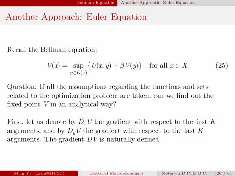
Recall the Bellman equation:
V(x) = supy∈G(x)
{U(x, y) + βV(y)} for all x ∈ X. (25)
Question: If all the assumptions regarding the functions and setsrelated to the optimization problem are taken, can we find out thefixed point V in an analytical way?
First, let us denote by DxU the gradient with respect to the first Karguments, and by DyU the gradient with respect to the last Karguments. The gradient DV is naturally defined.
Ming Yi (Econ@HUST) Doctoral Macroeconomics Notes on D.P. & O.C. 26 / 61

Bellman Equation Another Approach: Euler Equation
Another Approach: Euler Equation (Continued)
Suppose for an given x, y∗(x) ∈ G(x) solves the problem, then wemust have:
DyU(x, y∗(x)) + βDV(y∗(x)) = 0. (26)
The Euler equations above should hold for all x ∈ X.Also notice that V(x) = U (x, y∗(x)) + βV(y∗(x)) holds for allx ∈ X. Differentiating both sides with respect to x and inserting(26) into it yield (it could also be interpreted as an application ofthe Envelope Theorem with an interior solution assumed):
DV(x) =DxU(x, y∗(x)) +[∂y∗(x)∂x
]′[DyU(x, y∗(x)) + βDV(y∗(x))]
=DxU(x, y∗(x)) (27)
Ming Yi (Econ@HUST) Doctoral Macroeconomics Notes on D.P. & O.C. 27 / 61

Bellman Equation Another Approach: Euler Equation
Another Approach: Euler Equation (Continued)
Suppose for an given x, y∗(x) ∈ G(x) solves the problem, then wemust have:
DyU(x, y∗(x)) + βDV(y∗(x)) = 0. (26)
The Euler equations above should hold for all x ∈ X.
Also notice that V(x) = U (x, y∗(x)) + βV(y∗(x)) holds for allx ∈ X. Differentiating both sides with respect to x and inserting(26) into it yield (it could also be interpreted as an application ofthe Envelope Theorem with an interior solution assumed):
DV(x) =DxU(x, y∗(x)) +[∂y∗(x)∂x
]′[DyU(x, y∗(x)) + βDV(y∗(x))]
=DxU(x, y∗(x)) (27)
Ming Yi (Econ@HUST) Doctoral Macroeconomics Notes on D.P. & O.C. 27 / 61

Bellman Equation Another Approach: Euler Equation
Another Approach: Euler Equation (Continued)
Suppose for an given x, y∗(x) ∈ G(x) solves the problem, then wemust have:
DyU(x, y∗(x)) + βDV(y∗(x)) = 0. (26)
The Euler equations above should hold for all x ∈ X.Also notice that V(x) = U (x, y∗(x)) + βV(y∗(x)) holds for allx ∈ X. Differentiating both sides with respect to x and inserting(26) into it yield (it could also be interpreted as an application ofthe Envelope Theorem with an interior solution assumed):
DV(x) =DxU(x, y∗(x)) +[∂y∗(x)∂x
]′[DyU(x, y∗(x)) + βDV(y∗(x))]
=DxU(x, y∗(x)) (27)
Ming Yi (Econ@HUST) Doctoral Macroeconomics Notes on D.P. & O.C. 27 / 61

Bellman Equation Another Approach: Euler Equation
Another Approach: Euler Equation (Continued)
Reall y∗ maps X into X. Applying recursively Equation (27),DV(x) = DxU(x, y∗(x)), yields:
DV(y∗(x)) = DxU (y∗(x), y∗(y∗(x))) (28)
Denote y∗(x) = π(x), after inserting Equation (28) into (26), theEuler equations appears:
DyU(x, π(x)) + βDxU(π(x), π(π(x))) = 0, ∀x ∈ X. (29)
Ming Yi (Econ@HUST) Doctoral Macroeconomics Notes on D.P. & O.C. 28 / 61

Bellman Equation Another Approach: Euler Equation
Another Approach: Euler Equation (Continued)
When both x and y are variables (vectors with dimension 1), the Eulerequations are:
∂U(x(t), x∗(t + 1))
∂y + β∂U(x∗(t + 1), x∗(t + 2))
∂x = 0 (30)
The Euler equations themselves are only necessary condtions forthe problem, combining with the transversality condition
limt→∞
βtDxU(x∗(t), x∗(t + 1)) · x∗(t) = 0
makes them both necessary and sufficient conditions.If you are lucky enough, you can solve the problem using Eulerequations in a analytical and beautiful way, by correctly guessingthe form of the policy function.
Ming Yi (Econ@HUST) Doctoral Macroeconomics Notes on D.P. & O.C. 29 / 61

Bellman Equation Another Approach: Euler Equation
Another Approach: Euler Equation (Continued)
When both x and y are variables (vectors with dimension 1), the Eulerequations are:
∂U(x(t), x∗(t + 1))
∂y + β∂U(x∗(t + 1), x∗(t + 2))
∂x = 0 (30)
The Euler equations themselves are only necessary condtions forthe problem, combining with the transversality condition
limt→∞
βtDxU(x∗(t), x∗(t + 1)) · x∗(t) = 0
makes them both necessary and sufficient conditions.
If you are lucky enough, you can solve the problem using Eulerequations in a analytical and beautiful way, by correctly guessingthe form of the policy function.
Ming Yi (Econ@HUST) Doctoral Macroeconomics Notes on D.P. & O.C. 29 / 61

Bellman Equation Another Approach: Euler Equation
Another Approach: Euler Equation (Continued)
When both x and y are variables (vectors with dimension 1), the Eulerequations are:
∂U(x(t), x∗(t + 1))
∂y + β∂U(x∗(t + 1), x∗(t + 2))
∂x = 0 (30)
The Euler equations themselves are only necessary condtions forthe problem, combining with the transversality condition
limt→∞
βtDxU(x∗(t), x∗(t + 1)) · x∗(t) = 0
makes them both necessary and sufficient conditions.If you are lucky enough, you can solve the problem using Eulerequations in a analytical and beautiful way, by correctly guessingthe form of the policy function.
Ming Yi (Econ@HUST) Doctoral Macroeconomics Notes on D.P. & O.C. 29 / 61
Bellman Equation Another Approach: Euler Equation
Example 6.4
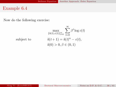
Now do the following exercise:
max{k(t),c(t)}∞t=0
∞∑t=0
βt log c(t)
subject to k(t + 1) = k(t)α − c(t),k(0) > 0, β ∈ (0, 1)
Method 1: Guess the policy function as π(x) = γxα, and verifyyour guess by determining the value of γ. (economic intuition?)Method 2: Guess the value function as V(x) = λ+ ξ log x, andverify your guess by determining the values of λ and ξ.You should find that the two methods above are equivalent.
Ming Yi (Econ@HUST) Doctoral Macroeconomics Notes on D.P. & O.C. 30 / 61

Bellman Equation Another Approach: Euler Equation
Example 6.4
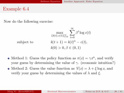
Now do the following exercise:
max{k(t),c(t)}∞t=0
∞∑t=0
βt log c(t)
subject to k(t + 1) = k(t)α − c(t),k(0) > 0, β ∈ (0, 1)
Method 1: Guess the policy function as π(x) = γxα, and verifyyour guess by determining the value of γ. (economic intuition?)
Method 2: Guess the value function as V(x) = λ+ ξ log x, andverify your guess by determining the values of λ and ξ.You should find that the two methods above are equivalent.
Ming Yi (Econ@HUST) Doctoral Macroeconomics Notes on D.P. & O.C. 30 / 61
Bellman Equation Another Approach: Euler Equation
Example 6.4
Now do the following exercise:
max{k(t),c(t)}∞t=0
∞∑t=0
βt log c(t)
subject to k(t + 1) = k(t)α − c(t),k(0) > 0, β ∈ (0, 1)
Method 1: Guess the policy function as π(x) = γxα, and verifyyour guess by determining the value of γ. (economic intuition?)Method 2: Guess the value function as V(x) = λ+ ξ log x, andverify your guess by determining the values of λ and ξ.
You should find that the two methods above are equivalent.
Ming Yi (Econ@HUST) Doctoral Macroeconomics Notes on D.P. & O.C. 30 / 61

Bellman Equation Another Approach: Euler Equation
Example 6.4
Now do the following exercise:
max{k(t),c(t)}∞t=0
∞∑t=0
βt log c(t)
subject to k(t + 1) = k(t)α − c(t),k(0) > 0, β ∈ (0, 1)
Method 1: Guess the policy function as π(x) = γxα, and verifyyour guess by determining the value of γ. (economic intuition?)Method 2: Guess the value function as V(x) = λ+ ξ log x, andverify your guess by determining the values of λ and ξ.You should find that the two methods above are equivalent.
Ming Yi (Econ@HUST) Doctoral Macroeconomics Notes on D.P. & O.C. 30 / 61

Bellman Equation Another Approach: Euler Equation
Guess and Verify
Question: If you have a guess that is successfully verified, can it bean incorrect one?
Answer: usually not in economic applications, especially afterassumptions (i)− (iv) have been made. The tough question here ishow would you know the specific form of the policy function (valuefunction) without any clue, for any given utility function?
Ming Yi (Econ@HUST) Doctoral Macroeconomics Notes on D.P. & O.C. 31 / 61

Bellman Equation Another Approach: Euler Equation
Guess and Verify
Question: If you have a guess that is successfully verified, can it bean incorrect one?Answer: usually not in economic applications, especially afterassumptions (i)− (iv) have been made. The tough question here ishow would you know the specific form of the policy function (valuefunction) without any clue, for any given utility function?
Ming Yi (Econ@HUST) Doctoral Macroeconomics Notes on D.P. & O.C. 31 / 61

Bellman Equation Miscellaneous Notes
Miscellaneous Notes
There are also tools for non-stationary dynamic programmingproblems.
What if there are noises in the problem, e.g., noises instate-evolution function f?Answer: E(·) appears in the objective function.What if the function f is totally unknown?Learn it from experience!Reinforcement Learning. Everybody is talking about ArtificialIntelligence and Machine Learning!
Ming Yi (Econ@HUST) Doctoral Macroeconomics Notes on D.P. & O.C. 32 / 61

Bellman Equation Miscellaneous Notes
Miscellaneous Notes
There are also tools for non-stationary dynamic programmingproblems.What if there are noises in the problem, e.g., noises instate-evolution function f?
Answer: E(·) appears in the objective function.What if the function f is totally unknown?Learn it from experience!Reinforcement Learning. Everybody is talking about ArtificialIntelligence and Machine Learning!
Ming Yi (Econ@HUST) Doctoral Macroeconomics Notes on D.P. & O.C. 32 / 61

Bellman Equation Miscellaneous Notes
Miscellaneous Notes
There are also tools for non-stationary dynamic programmingproblems.What if there are noises in the problem, e.g., noises instate-evolution function f?Answer: E(·) appears in the objective function.
What if the function f is totally unknown?Learn it from experience!Reinforcement Learning. Everybody is talking about ArtificialIntelligence and Machine Learning!
Ming Yi (Econ@HUST) Doctoral Macroeconomics Notes on D.P. & O.C. 32 / 61

Bellman Equation Miscellaneous Notes
Miscellaneous Notes
There are also tools for non-stationary dynamic programmingproblems.What if there are noises in the problem, e.g., noises instate-evolution function f?Answer: E(·) appears in the objective function.What if the function f is totally unknown?
Learn it from experience!Reinforcement Learning. Everybody is talking about ArtificialIntelligence and Machine Learning!
Ming Yi (Econ@HUST) Doctoral Macroeconomics Notes on D.P. & O.C. 32 / 61

Bellman Equation Miscellaneous Notes
Miscellaneous Notes
There are also tools for non-stationary dynamic programmingproblems.What if there are noises in the problem, e.g., noises instate-evolution function f?Answer: E(·) appears in the objective function.What if the function f is totally unknown?Learn it from experience!
Reinforcement Learning. Everybody is talking about ArtificialIntelligence and Machine Learning!
Ming Yi (Econ@HUST) Doctoral Macroeconomics Notes on D.P. & O.C. 32 / 61

Bellman Equation Miscellaneous Notes
Miscellaneous Notes
There are also tools for non-stationary dynamic programmingproblems.What if there are noises in the problem, e.g., noises instate-evolution function f?Answer: E(·) appears in the objective function.What if the function f is totally unknown?Learn it from experience!Reinforcement Learning. Everybody is talking about ArtificialIntelligence and Machine Learning!
Ming Yi (Econ@HUST) Doctoral Macroeconomics Notes on D.P. & O.C. 32 / 61

Bellman Equation Miscellaneous Notes
(a) AlphaGo by DeepMind (b) Goole Self-Driving Car
Figure 3: The A.I. mania relies intensively on tools provided by dynamic programming.
Ming Yi (Econ@HUST) Doctoral Macroeconomics Notes on D.P. & O.C. 33 / 61

Calculus of variations (变分法)
Calculus of variations (变分法)
A field of mathematical analysis that deals with maximizing orminimizing functionals, which are mappings from a set offunctions to the real numbers.Functionals are often expressed as definite integrals involvingfunctions and their derivatives. (e.g., the famous shortest (in time)path problem)A useful tool providing a necessary condition for finding anextrema, is the Euler-Lagrange equation.
Ming Yi (Econ@HUST) Doctoral Macroeconomics Notes on D.P. & O.C. 34 / 61

Calculus of variations (变分法) Euler-Lagrange equation
Euler-Lagrange equation
Intuition: Finding the extrema of functionals is similar to finding themaxima and minima of functions. This tool provides a link betweenthem to solve the problem. Consider the functional
J[x] =∫ t2
t1L(t, x(t), x ′(t)
)dt, (31)
wheret1, t2 are constants.x(t) is twice continuously differentiable.x ′(t) = dx
dt .L (t, x(t), x′(t)) is twice continuously differentiable with respect toall arguments.
Ming Yi (Econ@HUST) Doctoral Macroeconomics Notes on D.P. & O.C. 35 / 61

Calculus of variations (变分法) Euler-Lagrange equation
Euler-Lagrange equation (Continued)
If J [x] attains a local maximum at f, and η(t) is an arbitrary functionthat has at least one derivative and vanishes at the endpoints t1 and t2,then for any number ε → 0, we must have
J [f ] ≥ J [f + εη] . (32)
Term εη is called the variation of the function f. Now define
Φ(ε) = J[f + εη]. (33)
Since J [x] has a local maximum at x = f, it must be the case that Φ(ε)has a maximum at ε = 0 and thus
Φ′(0) =dΦdε
∣∣∣∣ε=0
=
∫ t2
t1
dLdε
∣∣∣∣ε=0
dt = 0. (34)
Ming Yi (Econ@HUST) Doctoral Macroeconomics Notes on D.P. & O.C. 36 / 61

Calculus of variations (变分法) Euler-Lagrange equation
Euler-Lagrange equation (Continued)Now taking total derivative of L [t, f + εη, (f + εη)′], we have:
dLdε =
∂L∂x η +
∂L∂x ′ η
′. (35)
Inserting (35) into (34) gives us
0 =
∫ t2
t1
dLdε
∣∣∣∣ε=0
dt =
∫ t2
t1
(∂L∂f η +
∂L∂f ′ η
′)
dt
=
∫ t2
t1
(∂L∂f η − η
d( ∂L∂f ′ )
dt
)dt + ∂L
∂f ′ η∣∣∣∣t2t1
=
∫ t2
t1η
(∂L∂f −
d( ∂L∂f ′ )
dt
)dt,
where the last two equalities use integration by parts and the fact thatη vanishes at t1 and t2.
Ming Yi (Econ@HUST) Doctoral Macroeconomics Notes on D.P. & O.C. 37 / 61

Calculus of variations (变分法) Euler-Lagrange equation
Euler-Lagrange equation (Continued)Now given ∫ t2
t1η
(∂L∂f −
d( ∂L∂f ′ )
dt
)dt = 0, (36)
the fundamental lemma of calculus of variations makes sure that
∂L∂f −
d( ∂L∂f ′ )
dt = 0 , ∀t ∈ (t1, t2) (37)
must hold!
However, it is possible to attain (37) based on (36) withoutapplying the lemma!A special form of η?
How about η(t) equals −(t − t1)(t − t2)[∂L∂f −
d( ∂L∂f ′ )
dt
]for t ∈ [t1, t2]
and 0 for t ∈ [t1, t2]?
Ming Yi (Econ@HUST) Doctoral Macroeconomics Notes on D.P. & O.C. 38 / 61

Calculus of variations (变分法) Euler-Lagrange equation
Euler-Lagrange equation (Continued)Now given ∫ t2
t1η
(∂L∂f −
d( ∂L∂f ′ )
dt
)dt = 0, (36)
the fundamental lemma of calculus of variations makes sure that
∂L∂f −
d( ∂L∂f ′ )
dt = 0 , ∀t ∈ (t1, t2) (37)
must hold!However, it is possible to attain (37) based on (36) withoutapplying the lemma!
A special form of η?
How about η(t) equals −(t − t1)(t − t2)[∂L∂f −
d( ∂L∂f ′ )
dt
]for t ∈ [t1, t2]
and 0 for t ∈ [t1, t2]?
Ming Yi (Econ@HUST) Doctoral Macroeconomics Notes on D.P. & O.C. 38 / 61

Calculus of variations (变分法) Euler-Lagrange equation
Euler-Lagrange equation (Continued)Now given ∫ t2
t1η
(∂L∂f −
d( ∂L∂f ′ )
dt
)dt = 0, (36)
the fundamental lemma of calculus of variations makes sure that
∂L∂f −
d( ∂L∂f ′ )
dt = 0 , ∀t ∈ (t1, t2) (37)
must hold!However, it is possible to attain (37) based on (36) withoutapplying the lemma!A special form of η?
How about η(t) equals −(t − t1)(t − t2)[∂L∂f −
d( ∂L∂f ′ )
dt
]for t ∈ [t1, t2]
and 0 for t ∈ [t1, t2]?Ming Yi (Econ@HUST) Doctoral Macroeconomics Notes on D.P. & O.C. 38 / 61
Calculus of variations (变分法) Euler-Lagrange equation
A simple exercise
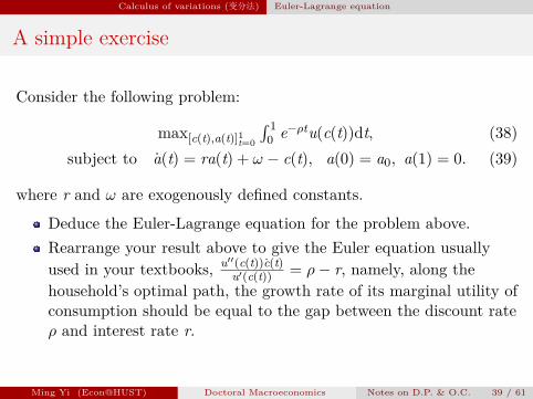
Consider the following problem:
max[c(t),a(t)]1t=0
∫ 10 e−ρtu(c(t))dt, (38)
subject to a(t) = ra(t) + ω − c(t), a(0) = a0, a(1) = 0. (39)
where r and ω are exogenously defined constants.
Deduce the Euler-Lagrange equation for the problem above.Rearrange your result above to give the Euler equation usuallyused in your textbooks, u′′(c(t))c(t)
u′(c(t)) = ρ− r, namely, along thehousehold’s optimal path, the growth rate of its marginal utility ofconsumption should be equal to the gap between the discount rateρ and interest rate r.
Ming Yi (Econ@HUST) Doctoral Macroeconomics Notes on D.P. & O.C. 39 / 61

Calculus of variations (变分法) Euler-Lagrange equation
Another exercise: the Brachistochrone Curve
The famous Brachistochrone Problem: given two points (x0, y0) and(x1, y1) with x0 < x1 and y0 > y1 in a two-dimensional world withgravitational acceleration g and without frictions . Find a smooth paththat connects these points and makes the travel time from (x0, y0) to(x1, y1) the shortest.The problem above is transformed into a mathematical one:
miny(x)
J(y) =∫ x1
x0
√1 + [y′(x)]2√
2g[y0 − y(x)]dx (40)
subject to y(x0) = y0, y(x1) = y1. (41)
Check outhttp://mathworld.wolfram.com/BrachistochroneProblem.html fora detailed introduction to this problem!
Ming Yi (Econ@HUST) Doctoral Macroeconomics Notes on D.P. & O.C. 40 / 61

Pontryagin’s Maximum Principle
Pontryagin’s Maximum Principle
Mainly developed by Pontryagin and his group.A Hamiltonian method that generalizes the Euler-Lagrangeequation above.
Ming Yi (Econ@HUST) Doctoral Macroeconomics Notes on D.P. & O.C. 41 / 61

Pontryagin’s Maximum Principle Variational Arguments
Variational ArgumentsProblem B1:
maxx(t),y(t),x1
W(x(t), y(t)) =∫ t1
0f(t, x(t), y(t))dt , (42)
subject to x(t) = g(t, x(t), y(t)), (43)x(0) = x0, and x(t1) = x1. (44)
Other settings:Continuous differentiability of functions are assumed again.the value of the state variable at the terminal of the horizon, x(t1),is flexible in this problem.We ignore here the trivial requirements stating that the values ofx(t) and y(t) should always be in some sets X ,Y ∈ R for all t.We suppose there exists an interior solution (x(t), y(t)), and focuson the necessary conditions for a solution.
Ming Yi (Econ@HUST) Doctoral Macroeconomics Notes on D.P. & O.C. 42 / 61

Pontryagin’s Maximum Principle Variational Arguments
Variational Arguments (Continued)
Take a variation of function y(t):
y(t, ϵ) = y(t) + ϵ η(t). (45)
Note that given y(t, ϵ), x(t) is now dependent on ϵ according toevolutionary equation (43), so the resulting x(t, ϵ) is defined by:
x(t, ϵ) = g(t, x(t, ϵ), y(t, ϵ)) for all t ∈ [0, t1], with x(0, ϵ) = x0. (46)
Define:
W(ϵ) = W(x(t, ϵ), y(t, ϵ))
=
∫ t1
0f(t, x(t, ϵ), y(t, ϵ))dt. (47)
Ming Yi (Econ@HUST) Doctoral Macroeconomics Notes on D.P. & O.C. 43 / 61

Pontryagin’s Maximum Principle Variational Arguments
Variational Arguments (Continued)
Since x(t), y(t) solve the optimal control problem, we must have:
W(ϵ) ≤ W(0) for all small engough ϵ → 0. (48)
Now recall that, g(t, x(t, ϵ), y(t, ϵ))− x(t, ϵ) = 0 holds for all t. Then forany function λ : [0, t1] → R, we must have:∫ t1
0λ(t)[g(t, x(t, ϵ), y(t, ϵ))− x(t, ϵ)]dt = 0. (49)
Function λ(t) is called the costate variable, with an interpretationsimilar to the Lagrange multipliers in standard (static) optimizationproblems.
Ming Yi (Econ@HUST) Doctoral Macroeconomics Notes on D.P. & O.C. 44 / 61

Pontryagin’s Maximum Principle Variational Arguments
Variational Arguments (Continued)
Combining (47) and (49) lets us redefine W(ϵ):
W(ϵ) =
∫ t1
0
f(t, x(t, ϵ), y(t, ϵ)) dt + 0
=
∫ t1
0
{f(t, x(t, ϵ), y(t, ϵ))+λ(t)[g(t, x(t, ϵ), y(t, ϵ))−x(t, ϵ)]}dt
=
∫ t1
0
{f(t, x(t, ϵ), y(t, ϵ))+λ(t)g(t, x(t, ϵ), y(t, ϵ))+λ(t)x(t, ϵ)}dt
−λ(t1)x(t1, ϵ) + λ(0)x0. (50)
The last equality above uses integration by parts.
Ming Yi (Econ@HUST) Doctoral Macroeconomics Notes on D.P. & O.C. 45 / 61

Pontryagin’s Maximum Principle Variational Arguments
Variational Arguments (Continued)Applying Leibniz’s Rule to (50) yields:
W ′(ϵ) =
∫ t1
0
[fx(t, x(t, ϵ), y(t, ϵ))+λ(t)gx(t, x(t, ϵ), y(t, ϵ))+λ(t)
]xϵ(t, ϵ)dt
+
∫ t1
0
[fy(t, x(t, ϵ), y(t, ϵ)) + λ(t)gy(t, x(t, ϵ), y(t, ϵ))] η(t)dt
−λ(t1)xϵ(t1, ϵ) (51)
Recall that condition (48) can be rewritten as W ′(0) = 0. We thushave:
0 =
∫ t1
0
[fx(t, x(t), y(t))+λ(t)gx(t, x(t), y(t))+λ(t)
]xϵ(t, 0)dt
+
∫ t1
0
[fy(t, x(t), y(t)) + λ(t)gy(t, x(t), y(t))] η(t)dt
−λ(t1)xϵ(t1, 0) (52)
Ming Yi (Econ@HUST) Doctoral Macroeconomics Notes on D.P. & O.C. 46 / 61

Pontryagin’s Maximum Principle Variational Arguments
Variational Arguments (Continued)Treating λ(t1)xϵ(t1, 0)
(52) must hold for any continuously differentiable λ(t).we simply focus on a class of costate variables satisfying
λ(t1) = 0 (53)
As a result, λ(t1)xϵ(t1, 0) = 0.
Ming Yi (Econ@HUST) Doctoral Macroeconomics Notes on D.P. & O.C. 47 / 61

Pontryagin’s Maximum Principle Variational Arguments
Variational Arguments (Continued)Treating
∫ t10
[fx(t, x(t), y(t))+λ(t)gx(t, x(t), y(t))+λ(t)
]xϵ(t, 0)dt
Besides λ(t1) = 0 as illustrated above, can we add morerequirements on the costate variable?Again, since (52) must hold for any continuously differentiableλ(t), why not focus on the following λ(t):
λ(t) = − [fx(t, x(t), y(t))+λ(t)gx(t, x(t), y(t))] , (54)λ(t1) = 0
Ming Yi (Econ@HUST) Doctoral Macroeconomics Notes on D.P. & O.C. 48 / 61

Pontryagin’s Maximum Principle Variational Arguments
Variational Arguments (Continued)Treating
∫ t10
[fy(t, x(t), y(t)) + λ(t)gy(t, x(t), y(t))] η(t)dt
Given the costate λ(t) defined above, equality∫ t10 [fy(t, x(t), y(t)) + λ(t)gy(t, x(t), y(t))] η(t)dt = 0 must hold for
arbitrary η(t).Applying the fundamental lemma of calculus of variations yields:
fy(t, x(t), y(t)) + λ(t)gy(t, x(t), y(t)) = 0 for all t ∈ [0, t1] (55)
Ming Yi (Econ@HUST) Doctoral Macroeconomics Notes on D.P. & O.C. 49 / 61

Pontryagin’s Maximum Principle Variational Arguments
Variational Arguments (Continued)
Theorem 3Suppose Problem B1 has an interior continuous solution (x(t), y(t)),then there exists a continuously differentiable costate λ(t) defined on[0, t1], such that (43), (53), (54), and (55) hold.
Ming Yi (Econ@HUST) Doctoral Macroeconomics Notes on D.P. & O.C. 50 / 61
Pontryagin’s Maximum Principle Variational Arguments
Problem B2
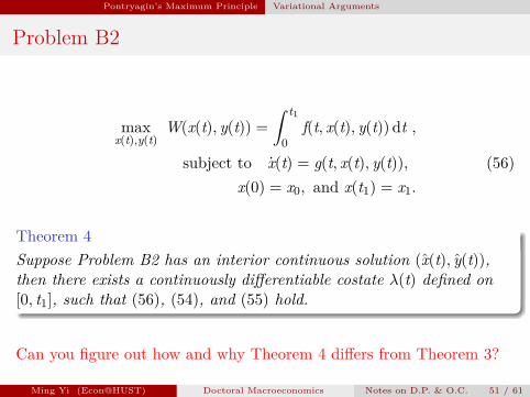
maxx(t),y(t)
W(x(t), y(t)) =∫ t1
0f(t, x(t), y(t))dt ,
subject to x(t) = g(t, x(t), y(t)), (56)x(0) = x0, and x(t1) = x1.
Theorem 4Suppose Problem B2 has an interior continuous solution (x(t), y(t)),then there exists a continuously differentiable costate λ(t) defined on[0, t1], such that (56), (54), and (55) hold.
Can you figure out how and why Theorem 4 differs from Theorem 3?
Ming Yi (Econ@HUST) Doctoral Macroeconomics Notes on D.P. & O.C. 51 / 61

Pontryagin’s Maximum Principle Variational Arguments
Revisiting the simple exercise
Consider the following problem:
max[c(t),a(t)]1t=0
∫ 10 e−ρtu(c(t))dt, (57)
subject to a(t) = ra(t) + ω − c(t), a(0) = a0, a(1) = 0. (58)
where r and ω are exogenously defined constants.
Use the Pontryagin’s Maximum Principle (Theorem 4 above) toget the same results (Euler equation) as before.Given u(c) = log(c), can you solve the problem above? What ifu(c) =
[θ − e−βc(t)]?
Ming Yi (Econ@HUST) Doctoral Macroeconomics Notes on D.P. & O.C. 52 / 61

Pontryagin’s Maximum Principle Variational Arguments
Problem B3
maxx(t),y(t)
W(x(t), y(t)) =∫ t1
0f(t, x(t), y(t))dt ,
subject to x(t) = g(t, x(t), y(t)), (59)x(0) = x0, and x(t1) ≥ x1.
Theorem 5Suppose Problem B3 has an interior continuous solution (x(t), y(t)),then there exists a continuously differentiable costate λ(t) defined on[0, t1], such that (59), (54), (55), and λ(t1)[x(t1)− x1] = 0 hold.
Can you figure out how and why Theorem 5 differs from Theorem 3?
Ming Yi (Econ@HUST) Doctoral Macroeconomics Notes on D.P. & O.C. 53 / 61

Pontryagin’s Maximum Principle Pontryagin’s Maximum Principle
Pontryagin’s Maximum PrincipleRevisit Problem B1. Define the Hamiltonian:
H(t, x(t), y(t), λ(t)) ≡ f(t, x(t), y(t)) + λ(t)g(t, x(t), y(t)). (60)
Theorem 6Suppose Problem B1 has an interior continuous solution (x(t), y(t)),then there exists a continuously differentiable function λ(t) such thatthe following necessary conditions hold:
λ(t) = −Hx(t, x(t), y(t), λ(t)) for all t ∈ [0, t1], (61)x(t) = Hλ(t, x(t), y(t), λ(t)) for all t ∈ [0, t1], (62)
H(t, x(t), y(t), λ(t)) ≥ H(t, x(t), y, λ(t)) for all feasible y, t, (63)x(0) = x0, λ(t1) = 0. (64)
Question: relationship between (55) and (63)?Ming Yi (Econ@HUST) Doctoral Macroeconomics Notes on D.P. & O.C. 54 / 61

Pontryagin’s Maximum Principle Pontryagin’s Maximum Principle
Pontryagin’s Maximum Principle (Continued)
The results of equations (61)-(64) are straightforward tounderstand given the variational arguments illustrated earlier.Can you figure out the Pontryagin’s Maximum Principle forProblems B2 and B3?(important) In all problems so far, we have both x and yone-dimensional variables. The Pontryagin’s maximum Principlealso applies to scenarios where x and y are actually vectors ofstate and control variables, respectively. In these cases, it may benecessary to introduce more than one costate variables, e.g.,λ1(t), · · · , λk(t) into the Hamiltonian. For instance, if theevolutionary equation becomes x = g1(·) and d2x
dt2 = g2(·). Weactually have two state variables here: x = (x, x).So far only necessary conditions discussed. Sufficient conditions?It suffices to have some degree of concavity of H(t, x, y, λ) in (x, y).
Ming Yi (Econ@HUST) Doctoral Macroeconomics Notes on D.P. & O.C. 55 / 61

Pontryagin’s Maximum Principle Infinite Horizon
Infinite Horizon Problem
Consider Problem B4:
maxx(t),y(t)
W(x(t), y(t)) =∫ ∞
0f(t, x(t), y(t))dt , (65)
subject to x(t) = g(t, x(t), y(t)), (66)x(0) = x0, and lim
t→∞b(t)x(t) ≥ x1.
Notice: When the integral is defined on an unbounded interval, weneed more assumptions (related to the dominated convergencetheorem) on the integrability of some functions for the Leibniz’s Ruleto apply. However, these details are trivial and almost always satisfiedin economic applications.
Ming Yi (Econ@HUST) Doctoral Macroeconomics Notes on D.P. & O.C. 56 / 61

Pontryagin’s Maximum Principle Infinite Horizon
Infinite Horizon Problem (continued)
Theorem 7Suppose Problem B4 has an interior continuous solution (x(t), y(t)),then there exists a continuously differentiable function λ(t) such thatthe following necessary conditions hold:
λ(t) = −Hx(t, x(t), y(t), λ(t)) for all t ∈ R+, (67)x(t) = Hλ(t, x(t), y(t), λ(t)) for all t ∈ R+, (68)
H(t, x(t), y(t), λ(t)) ≥ H(t, x(t), y, λ(t)) for all feasible y, t, (69)x(0) = x0, lim
t→∞b(t)x(t) ≥ x1. (70)
Ming Yi (Econ@HUST) Doctoral Macroeconomics Notes on D.P. & O.C. 57 / 61

Pontryagin’s Maximum Principle Current-Value Hamiltonian
Current-Value Hamiltonian
Consider Problem B5:
maxx(t),y(t)
W(x(t), y(t)) =∫ ∞
0e−ρtf(x(t), y(t))dt , (71)
subject to x(t) = g(t, x(t), y(t)), (72)x(0) = x0, and lim
t→∞b(t)x(t) ≥ x1.
The Hamiltonian is:
H(t, x(t), y(t), λ(t)) = e−ρt [f(x(t), y(t)) + eρtλ(t)g(t, x(t), y(t))]
(73)
Define function µ(t) ≡ eρtλ(t). The current-value Hamiltonian isthus defined as
H(t, x(t), y(t), µ(t)) ≡ f(x(t), y(t)) + µ(t)g(t, x(t), y(t)). (74)
Ming Yi (Econ@HUST) Doctoral Macroeconomics Notes on D.P. & O.C. 58 / 61
Pontryagin’s Maximum Principle Current-Value Hamiltonian
Current-Value Hamiltonian(continued)
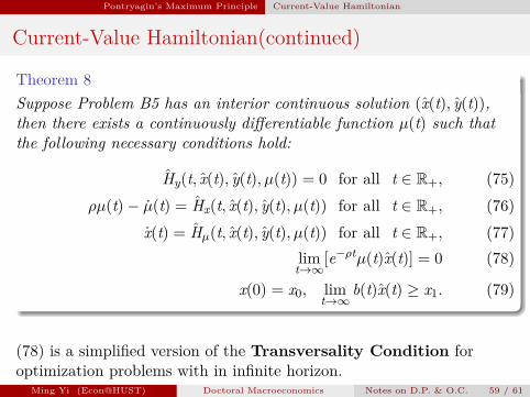
Theorem 8Suppose Problem B5 has an interior continuous solution (x(t), y(t)),then there exists a continuously differentiable function µ(t) such thatthe following necessary conditions hold:
Hy(t, x(t), y(t), µ(t)) = 0 for all t ∈ R+, (75)ρµ(t)− µ(t) = Hx(t, x(t), y(t), µ(t)) for all t ∈ R+, (76)
x(t) = Hµ(t, x(t), y(t), µ(t)) for all t ∈ R+, (77)lim
t→∞[e−ρtµ(t)x(t)] = 0 (78)
x(0) = x0, limt→∞
b(t)x(t) ≥ x1. (79)
(78) is a simplified version of the Transversality Condition foroptimization problems with in infinite horizon.
Ming Yi (Econ@HUST) Doctoral Macroeconomics Notes on D.P. & O.C. 59 / 61

Pontryagin’s Maximum Principle Homework
Homework
Try your best to understand:Example 7.1 (page 233), Example 7.3 (page 252), and Section 7.8:The q-theory (page 269) in Acemoglu (2008).Or examples between pages 641-643, and Section 20.5 (page 649)in Chiang and Wainwright (2005). Note that the notations used inthese books are different.
Ming Yi (Econ@HUST) Doctoral Macroeconomics Notes on D.P. & O.C. 60 / 61

References
References
[1] Acemoglu, D. (2008). Introduction to modern economic growth,Princeton University Press.
[2] Chiang, A. and Wainwright, K. (2005). Fundamental Methods ofMathematical Economics, McGraw-Hill higher education,McGraw-Hill.
Ming Yi (Econ@HUST) Doctoral Macroeconomics Notes on D.P. & O.C. 61 / 61