dynamic positioning conference october 9-10, 2007 design

Return to Session Directory Doug Phillips Failure is an Option

DYNAMIC POSITIONING CONFERENCE October 9-10, 2007

Design & Control

Exponentially Stable Underactuated Dynamic

Positioning of Marine Vehicle

Matthew Greytak, Franz Hover Massachusetts Institute of Technology

Return to Session Directory

Matthew Greytak DP 2007 Design & Control Underactuated Dynamic Positioning

DP Conference Houston October 9-10, 2007 Page 1

Abstract Dynamic positioning is mostly limited to fully actuated vessels. However many vessels, especially small ones, are underactuated with only two control inputs (throttle and rudder angle). We present an exponentially stable control system for dynamic positioning of an underactuated marine vehicle. A state feedback controller, such as a linear quadratic regulator (LQR), controls the heading of the vehicle and the longitudinal error relative to the desired position. For certain initial conditions the final transverse error will also be zero. These initial conditions form a manifold in the state space. A separate manifold convergence controller drives the vehicle states toward this manifold. Both controllers converge when the vehicle is at the desired position and orientation. Convergence of the state feedback controller within a large calculable region of the state space is proven using contraction analysis. The performance of the control system is demonstrated with simulations and with experiments using a 3.71-meter autonomous surface vessel.

1. Introduction Dynamic positioning refers to the active control of a marine surface vessel such that it remains at a fixed position and orientation without the use of moorings. Positioning without moorings is an attractive option for offshore drilling platforms and dive support because water depth is not an issue and repositioning to a new location is easy [1]. Vessels designed for dynamic positioning are fully actuated with many independent thrusters, and the control challenge is thrust allocation between the various control channels. Many surface vessels are underactuated with only two independent control channels (throttle and rudder angle for example). This is especially true for smaller vessels. Underactuated dynamic positioning (also known as underactuated point stabilization) is not possible with a fixed continuous state feedback law [2]. However the underactuated vessel is small-time locally controllable [3, 4]. It is shown in [3] that Lie brackets of differential rotation matrices span the entire space of desired motion vectors. This observation leads directly to control laws with small amplitude oscillations to repeatedly apply the Lie bracket-based motions to the system states. Specifically, [3-5] use a periodic time-varying control law to stabilize the averaged system; each period of control oscillation brings the system slightly closer to the origin. Another reference [6] uses a switched seesaw unstable/stable control law for stabilization. Yet another [7] uses virtual velocity controls as an intermediate step in the control law. Several solutions are presented in [8] for a simplified hovercraft model (no damping terms). All of these methods exhibit an undesirable oscillatory behavior of the controller inputs and state outputs even in the absence of noise or disturbances. Some solutions to this problem neglect the dynamics of the vessel, assuming small velocities and/or a fully symmetric vessel [3, 4, 8]. Furthermore, all of the aforementioned references assume that a surge force and yaw moment are the two control inputs, with neither input affecting sway. For most practical vessel configurations this is an unreasonable assumption unless the vessel is steered with differential thrust on two fore- or aft-facing propellers. That is not a common thruster configuration for most marine vehicles. In this paper we acknowledge that the mechanism that generates a yaw moment may also generate a sway force, such as with a rudder or azimuthing thruster. In Section 2 we derive a nonlinear state space formulation for the surface vessel equations of motion and kinematics. In Section 3 we show how a state feedback controller can potentially stabilize almost all of the vessel states in a computable region of the state space. This controller, acting alone, drives the vessel to the correct orientation along a line passing through the goal position. For



certain initial conditions this state feedback controller drives the vessel exactly to the goal in the absence of disturbances. That particular set of initial conditions forms a manifold in the state space. In Section 4 we derive an algorithm to move the vessel toward this manifold while the state feedback controller is running. In Section 5 we present simulation results demonstrating the overall algorithm. Experiments were performed using a 3.71-meter autonomous surface vessel; the results of these experiments are presented in Section 6.

2. Mathematical Surface Vessel Model We present a nonlinear state-space model for the vessel dynamics and a convenient coordinate transformation to map the global position onto a vessel-rotated frame. The model described here is used in the state feedback control law of Section 3 and the manifold convergence controller of Section 4.

2.1 Equations of motion

Borrowing Fossen's notation [1], the equations of motion for the vessel take the form:

!

˙ " = a "( )" + b# (1)

˙ $ = J $( )" (2)

where

!

" = u , v , r[ ]T (vessel frame surge, sway and yaw velocities) and

!

" = X ,Y ,#[ ]T (global Cartesian

frame position and orientation with the X axis pointing East and the Y axis pointing North). The hydrodynamic damping and Coriolis terms are included in

!

a "( )" . We assume that the mass matrix is diagonal. The system is underactuated if the rank of b is less than 3 or if the size of τ is less than 3. The position and heading of the boat are (X,Y,ψ) in the global frame and (z1,z2,ψ) in a frame centered at the origin but rotated by an angle ψ:

!

z1 = X cos" +Y sin"

z2 = #X sin" +Y cos"(3)

These coordinates are shown in Figure 1.

Figure 1: Global and rotated coordinate frames.



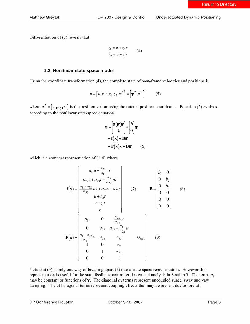
Differentiation of (3) reveals that

!

˙ z 1 = u + z2r

˙ z 2 = v " z1r(4)

2.2 Nonlinear state space model Using the coordinate transformation (4), the complete state of boat-frame velocities and positions is

!

x = u,v,r,z1,z2,"[ ]T

# $ T,zT[ ]

T

(5)

where

!

zT = z

1, z2,"[ ] is the position vector using the rotated position coordinates. Equation (5) evolves

according to the nonlinear state-space equation

!

˙ x =a "( )"

˙ z

#

$ %

&

' ( +

b

0

#

$ % &

' ( )

* f x( )+ B)

* F x( )x + B) (6)

which is a compact representation of (1-4) where

!

f x( ) =

a11u +m22

m11

vr

a22v + a23r "m11

m22

ur

m11"m22

m33

uv + a32v + a33r

u + z2r

v " z1r

r

#

$

% % % % % % % % %

&

'

( ( ( ( ( ( ( ( (

(7) B =

b1 0

0 b2

0 b3

0 0

0 0

0 0

#

$

% % % % % % %

&

'

( ( ( ( ( ( (

(8)

F x( ) =

a11 0m22

m11

v

0 a22 a23 "m11

m22

u

m11"m22

m33

v a32 a33

1 0 z2

0 1 "z10 0 1

06)3

#

$

% % % % % % % % %

&

'

( ( ( ( ( ( ( ( (

(9)

Note that (9) is only one way of breaking apart (7) into a state-space representation. However this representation is useful for the state feedback controller design and analysis in Section 3. The terms aij may be constant or functions of ν . The diagonal aii terms represent uncoupled surge, sway and yaw damping. The off-diagonal terms represent coupling effects that may be present due to fore-aft



asymmetry (a sway acceleration due to yaw velocity and vice versa). There are no terms a12, a21, a13 or a31 because we assume port-starboard symmetry. The goal of dynamic positioning is for the velocities

!

u , v , r{ } = 0 and the global positions

!

X,Y ,"{ } = 0. A coordinate transformation can map any other goal position to the origin. Using the state vector representation in (5) with the coordinate rotation in (3), we note that an equivalent goal is

!

x = 0.

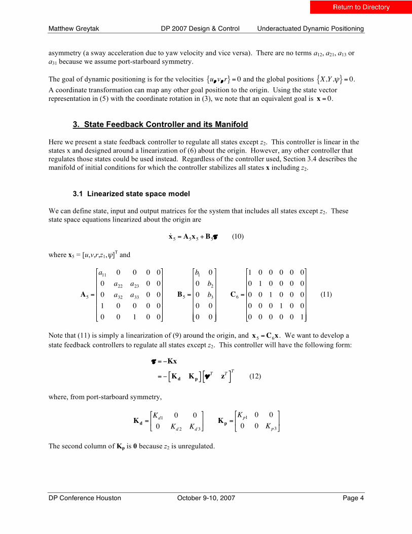
3. State Feedback Controller and its Manifold Here we present a state feedback controller to regulate all states except z2. This controller is linear in the states x and designed around a linearization of (6) about the origin. However, any other controller that regulates those states could be used instead. Regardless of the controller used, Section 3.4 describes the manifold of initial conditions for which the controller stabilizes all states x including z2.

3.1 Linearized state space model We can define state, input and output matrices for the system that includes all states except z2. These state space equations linearized about the origin are

!

˙ x 5 = A5x5 + B5" (10)

where x5 = [u,v,r,z1,ψ]T and

!

A5 =

a11 0 0 0 0

0 a22 a23 0 0

0 a32 a33 0 0

1 0 0 0 0

0 0 1 0 0

"

#

$ $ $ $ $ $

%

&

' ' ' ' ' '

B5 =

b1 0

0 b2

0 b3

0 0

0 0

"

#

$ $ $ $ $ $

%

&

' ' ' ' ' '

C6 =

1 0 0 0 0 0

0 1 0 0 0 0

0 0 1 0 0 0

0 0 0 1 0 0

0 0 0 0 0 1

"

#

$ $ $ $ $ $

%

&

' ' ' ' ' '

(11)

Note that (11) is simply a linearization of (9) around the origin, and

!

x5

=C6x . We want to develop a

state feedback controllers to regulate all states except z2. This controller will have the following form:

!

" = #Kx

= # Kd Kp[ ] $TzT[ ]

T

(12)

where, from port-starboard symmetry,

!

Kd =Kd1 0 0

0 Kd 2 Kd 3

"

# $

%

& ' Kp =

Kp1 0 0

0 0 Kp3

"

# $

%

& '

The second column of Kp is 0 because z2 is unregulated.



3.2 Linear quadratic regulator (LQR) One way to design this state feedback controller is to use a linear quadratic regulator (LQR). For an LQR we want to minimize the following cost function:

!

J = x5TQ5x5 + " T

R" dt0

#

$ (13)

where Q5 and R are diagonal weighting matrices of appropriate size. We achieve a minimum of J using state feedback when

!

" = #R#1BTC6

T

P5C6x (14)

$ #Kx

where P5 is the solution to the algebraic Riccati equation:

!

A5

T

P5

+P5A5"P

5B5R"1B5P5

+Q5

= 0

Recall that C6 is an output matrix for all states except z2, used here simply to expand from partial state feedback (with x5) to full state feedback (with x).

3.3 Stability of the nonlinear closed-loop system

When using state feedback control the nonlinear closed loop dynamics follow the equation

!

˙ x = f x( )"BKx

# fcl

x( )

= F x( )"BK( )x

# Fcl

x( )x (15)

The state feedback controller is designed for the linear state transition matrix (11). However the controller is applied to the nonlinear state transition matrix (9). Through the controller design we know that the linearized closed-loop state transition matrix

!

C6

TA5C6"BK is a constant matrix whose

eigenvalues all have negative real parts (except for the eigenvalue at the origin corresponding to the z2 state) but the actual closed-loop state transition matrix Fcl(x) is state-dependent. The state feedback controller is guaranteed to be stable in a neighborhood around the origin, due to the design of the controller, but we would like to be able to use the controller over a wider range of the state space. Both [9] and [10] address this problem using contraction analysis. A system is said to be contracting if, in that region, the Jacobian of fcl(x) is negative definite. More generally, a system is contracting if

!

˙ M + M" f

cl

" x+" f

cl

" x

#

$ %

&

' (

T

M < 0 (16)



for some metric M. (Reference [9] restricts M to be constant in time and refers to (16) as the Demidovich condition.) If there is a fixed point in the region of contraction then all trajectories starting in that region converge to the fixed point. For the closed loop system (15) this fixed point is the origin. The region of contraction is highly dependent on the choice of the metric M. Finding the optimal choice of this metric (that which gives the largest region of contraction) is a nonlinear optimization problem. In the absence of an analytic solution we would need to sample the state space to check the contraction condition (16) using our choice of M. It takes just as much computational effort to simply simulate the controller starting from the same grid of points in the state space to verify if the system stabilizes (except for z2) after some appropriately large amount of time. For this system the region of convergence is mostly a function of v and z2. The white space in Figure 2 shows the region of convergence for the vessel described in Section 5 over the entire sample space of u, r, z1 and ψ based on simulations of 200 seconds of closed-loop control. In the white region all of the x5 states had converged to the origin within a small tolerance and z2 and converged to a constant value.

Figure 2: The white space represents the states for which the closed-loop state feedback control system drives the x5 states to the origin. This plot shows a projection of the 6D x-space onto the (v, z2) plane.

3.4 Manifold of initial conditions Using the state feedback controller described in Section 3.2, or any other stable controller, u, v, r, z1 and ψ are regulated to zero as long as the states remain inside a computable region of convergence. The transverse position z2 will converge to a constant value as long as the other states are driven to zero. In the global frame the vessel will end up on the global Y axis pointing in the ψ = 0 direction. The steady-state z2 position (which equals the global Y position if z1 and ψ have been driven to zero) is a function of the initial conditions when the state feedback controller was switched on. That is, for any initial

!

x( t = 0) we know that the final state

!

x( t =") is

!

x "( ) = 0 0 0 0 z2 "( ) 0[ ]T

(17) The goal of dynamic positioning is for

!

x = 0, so an interesting set of initial conditions is the set for which

!

z2" # z2 "( ) = 0 given the state feedback controller designed in (12) (or any other stable controller). This

set forms a manifold in the state space. If the vessel state is on this manifold we can use the state



feedback controller to drive to the origin of the state space. The manifold convergence controller described in the next section is used to drive the vessel state toward this manifold. It is not possible to compute the location and shape of the manifold directly but for any initial state x(0) the expected final z2 value can be computed with a single forward simulation. This simulation includes the equations of motion and the control law but also any control limits, delays or known external environmental forces such as current or wind that may be present. The manifold for the experimental ship model from Section 5 is shown in Figure 3.

Figure 3: Manifold of initial conditions (u, v, r = 0) for which

!

z2"

= 0. The blue line represents the set of global initial conditions (0, Y, 0) for which

!

z2"

is trivially zero. This manifold is an isosurface of volume data, as it cannot be computed directly.

4. Manifold Convergence Controller (MCC)

We would like to augment the state feedback control law

!

" = "SF

= #Kx (14) with an extra control effort

!

"MC

to drive

!

z2"

to zero:

!

" = "SF

+ "MC

= #Kx + "MC

(18)

This control division (18) requires that the plant be linear in the control inputs. Our task is to derive a manifold convergence controller (MCC) for

!

"MC

. We define a positive definite Lyapunov function V that is zero on the manifold and positive elsewhere:

!

V =1

2z2"

2(19)

To monotonically converge to the manifold we need

!

˙ V , the time derivative of (19), to be a negative definite function. To get access to the inputs

!

"MC

we can represent

!

˙ V in the following way:



!

˙ V ="V

"x

dx

dt

="V

"xF x( )#BK( )x +B$

MC[ ]

= z2%

"z2%

"xF x( )#BK( )x +B$

MC[ ] = cv

(20)

where cv is a strictly negative scalar function of V and it is assumed that the state feedback controller is running the whole time. Rearranging we get

!

z2"#z2"

#xB$

MC= c

v% z2"

#z2"

#xF x( )%BK( )x (21)

which has the form

!

G"MC

= cv#Hx (22)

where

!

G " z2# $z2# $x( )B is a 1x2 vector,

!

"MC

is the 2x1 vector of inputs,

!

H " z2# $z2# $x( ) F x( )%BK( )

is a 1x6 vector, and both sides of (22) evaluate to a scalar. This equation can be solved for the inputs

!

"MC

using the pseudoinverse:

!

" MC = pinv G( ) cv # H( )x[ ] (23)

For a uniform rate of convergence to the manifold, cv can be a negative constant, and for first-order exponential convergence we set it equal to –V/TV where TV is a positive constant; then the function V will decay according to

!

V t( ) =V0e"t / T

V . In this latter case the input vector is:

!

" MC = #pinv$z2%$x

B&

' (

)

* + 1

2TVz2% +

$z2%$x

F x( )#BK( )x,

- .

/

0 1 (24)

The time constant TV need not be constant as long as

!

"t, TVt( ) > 0 . For a small TV the manifold

convergence controller drives the vessel state toward the manifold quickly using a large control effort, and for large TV the state moves toward the manifold more gradually. The derivatives

!

"z2# / "x can be computed by evaluating

!

z2"

at small perturbed values around the state x. Each evaluation is a forward simulation in time, including any control limits or known environmental disturbances as in Section 3.4. In each time step of the MCC, the forward simulation must be run seven times (one nominal plus six perturbations) to evaluate

!

"z2# / "x .

The MCC (24) constantly tries to improve the predicted future value of z2. Even if the state feedback controller is running at the same time, as in (18), the net effect may be to temporarily perturb the other states away from the origin in order to improve the predicted future steady-state position. To prevent a limit cycle the MCC must be switched off when

!

z2" drops below some positive value

!

z2tol1

. Then under the state feedback controller alone the vessel will now drive the states to



!

x "( ) = 0 0 0 0 z2tol1

0[ ]T

assuming no modeling error or disturbances. To account for modeling errors or disturbances we can choose a larger positive threshold

!

z2tol2

such that if the predicted value

!

z2" grows past

!

z2tol2

then the MCC is switched back on. This behavior is illustrated in Figure 4. In essence this means that the overall control system will try to deal with small disturbances with the state feedback controller but it will turn on the MCC to reposition itself in the presence of larger disturbances that push the vessel states away from the origin.

Figure 4: Hysteresis switching behavior for the manifold convergence controller.

!

z2tol1

defines the ultimate positioning accuracy and

!

z2tol2

defines the robustness to disturbances and modeling error.

5. Simulation In a simulation of the underactuated dynamic positioning algorithm we used a linear plant model for the 3.71-meter experimental vessel from Section 6 with no cross-terms (a fore-aft symmetry approximation). In this model a11 = -0.10 [s-1], a22 = -0.17 [s-1], a33 = -0.50 [s-1], a23 = a32 = 0, b1 = 0.20 [kg-1], b2 = 0.11 [kg-1], b3 = -0.18 [kg-1m-1], m11 = 145 [kg], m22 = 209 [kg] and m33 = 163 [kg m2]. An LQR was designed with Q5 = diag([1,0,1,1,10]) and R = diag([10,10]). The time constant for the MCC was TV = 5 [s]. In the simulation we used tight switching tolerances:

!

z2tol1

= 0.1 [m] and

!

z2tol2

= 0.2 [m].

Figure 5: Simulated trajectory converging to the origin. The arrows indicate the vessel heading at 2-second intervals.



Figure 5 shows the simulated trajectory starting from an initial global position of (X, Y, ψ) = (-2, -1, π/2) and driving to the origin (0, 0, 0). After 50 seconds of simulation the vessel is at the global position (0.011, 0.092, 0.000). In that time the X position has almost completely converged, the Y position has settled just inside the switching tolerance

!

z2tol1

, and the heading has completely converged. The corresponding control inputs are plotted in Figure 6.

Figure 6: Control inputs τx and τy from the simulation. Note the change in behavior at t = 26 seconds when the MCC is switched off. Figure 7 shows the convergence of the Lyapunov function V. Note that except for the first few seconds (during which the throttle hits its saturation limit) this function exhibits exponential decay. After 26 seconds V drops below

!

Vtol

=1

2z2tol1

2= 0.005 [m2] and remains constant thereafter.

Figure 7: Exponential decay of the Lyapunov function V with a time constant TV = 5 [s].

6. Experimental Results

Experiments were performed with the autonomous surface vessel depicted in Figure 8. It is a 3.71-meter kayak hull powered by a single azimuthing thruster. It is controlled by an onboard PC/104 660 MHz Pentium III CPU running Mathworks’ xPC Target real-time operating system. Sensors include a tilt-compensated 3-axis magnetometer and a WAAS-enabled GPS sensor. The linear vessel model is provided in the previous section. Experiments were performed in the Charles River in Boston, Massachusetts.



Figure 8: Autonomous surface vessel driving in the Charles River in Boston, Massachusetts.

The control parameters for the experiments are the same as for the simulation in the previous section except the switching tolerances were increased to

!

z2tol1

= 1.0 [m] and

!

z2tol2

= 2.0 [m] because of wind and wave disturbances and modeling error. During the experiment the wind was from the SE at 3-5 knots. The heading is plotted in Figure 9 and the position errors are plotted in Figure 10. The heading error never exceeds 45° and the position errors stay within one boatlength.

Figure 9: Heading errors during the experiment.



Figure 10: Global (X,Y) position errors during the experiment.

Figure 11 shows the vessel trajectory from t = 40 [s] to t = 80 [s], starting from the global position (14.9, 0.1, -52°) and driving to the reference position (15, -10, 0°). Initially the vessel is outside the outer switching boundary. The MCC switches on to drive

!

z2"

back inside the inner switching boundary. The MCC briefly switches back on to correct for wind and modeling error which have pushed the

!

z2"

prediction back outside

!

z2tol2

. Then the MCC switches off and the state feedback controller drives the vessel to the goal. The final position error is due to a wind force that was not programmed into the forward simulation in the control law (24).

7. Conclusions We have presented a controller to stabilize the position and orientation of an underactuated surface vessel. The controller works in two parts:

• Use a manifold convergence controller (MCC) to exponentially converge to within a nonzero tolerance of a particular manifold of the state space, then

• Turn off the MCC and drive along the manifold to the goal configuration using a state feedback controller.

A hysteresis switching law turns the MCC on and off in a robust manner. The overall behavior is intuitive in the presence of environmental disturbances. For small disturbances the state feedback controller deals with the state errors as well as possible, ignoring lateral position error. For larger disturbances the vessel uses the MCC to reposition and drive back to the goal. The drawback of this switching law is that the predicted final position error is bounded within

!

z2tol1

instead of being driven exactly to zero. When the state feedback controller is running alone, the state

!

z2 is unregulated and the predicted final

(

!

t =") value

!

z2" is constant in the absence of disturbances or modeling error. However, all of the other

states are regulated to zero. When additionally the MCC is running,

!

z2" is driven exponentially toward

zero. To accomplish this the other x5 states may be perturbed away from the origin. Once the MCC drives

!

z2" below

!

z2tol1

it turns off and the remaining states are regulated to zero by the state feedback controller. In this way either the future error state

!

z2" or the current states x5 are regulated at any

particular time, with the overall result that the vessel converges to the origin of the state space. The time



constant for the

!

z2" convergence when the MCC is running is explicitly TV. When the MCC is not

running the time constants for the convergence of the other states are a function of the state feedback controller parameters (Q5 in the case of the LQR). Depending on the ratio of MCC to state feedback time constants the controller will either be more or less aggressive about reducing

!

z2" at the expense of the x5

states. The choice of time constants is a design parameter that determines the speed and fluidity with which the vessel drives to the origin.

Figure 11: Vessel trajectory from t = 40 [s] to 80 [s] during the experiment (unfiltered GPS position). The arrows indicate the vessel heading at 2-second intervals. The switching behavior is indicated in the figure. The circle indicates the goal position (pointing East, along the X-axis). The MCC relies on a forward simulation of the nonlinear vessel equations of motion, control constraints and known environmental disturbances. The performance of this algorithm degrades with modeling error, so a logical extension of the algorithm is to add adaptation to learn the dynamic model and steady environmental forces in real-time. We are currently exploring extensions of this algorithm to 5 degree of freedom underactuated positioning (position, heading, and pitch) of an autonomous underwater vehicle using three control inputs (surge force, yaw moment, and pitch moment). Initial simulations indicate that the same formulation can be extended to the 5D case with almost no adjustments just as [11] extended the planar results of [4] to 5 degrees of freedom.



References

1. Fossen, T.I., Marine Control Systems: Guidance, Navigation, and Control of Ships, Rigs and

Underwater Vehicles. 2002, Trondheim, Norway: Marine Cybernetics. 2. Brockett, R.W., Asymptotic stability and feedback stabilization. Differential Geometric Control

Theory, 1983. 27: p. 181–191. 3. Leonard, N.E., Control synthesis and adaptation for an underactuated autonomous underwater

vehicle. IEEE Journal of Oceanic Engineering, , 1995. 20(3): p. 211-220. 4. Pettersen, K.Y. and O. Egeland. Exponential stabilization of an underactuated surface vessel. in

Proceedings of the 35th IEEE Conference on Decision and Control. 1996. 5. Pettersen, K.Y. and T.I. Fossen, Underactuated dynamic positioning of a ship-experimental

results. IEEE Transactions on Control Systems Technology, , 2000. 8(5): p. 856-863. 6. Aguiar, A.P., J.P. Hespanha, and A.M. Pascoal. Stability of switched seesaw systems with

application to the stabilization of underactuated vehicles. in 44th IEEE Conference on Decision and Control and 2005 European Control Conference. 2005.

7. Do, K.D., Z.P. Jiang, and J. Pan, Universal controllers for stabilization and tracking of underactuated ships. Systems and Control Letters, 2002. 47(4): p. 299-317.

8. Fantoni, I. and R. Lozano, Non-linear Control for Underactuated Mechanical Systems. 2002, London: Springer-Verlag London Ltd.

9. Pavlov, A., N. van de Wouw, and H. Nijmeijer, The local output regulation problem: convergence region estimates. IEEE Transactions on Automatic Control, 2004. 49(5): p. 814-819.

10. Lohmiller, W. and J.-J.E. Slotine, On contraction analysis for non-linear systems. Automatica, 1998. 34(6): p. 683-696.

11. Pettersen, K.Y. and O. Egeland, Time-varying exponential stabilization of the position and attitude of an underactuated autonomous underwater vehicle. IEEE Transactions on Automatic Control, 1999. 44(1): p. 112-115.

dynamic positioning conference october 9-10, 2007 design

Documents