dynamic neural networks for real-time water level predictions

HESSD7, 2317–2345, 2010

Dynamic neuralnetworks for

real-time water levelpredictions

Y.-M. Chiang et al.

Title Page

Abstract Introduction

Conclusions References

Tables Figures

J I

J I

Back Close

Full Screen / Esc

Printer-friendly Version

Interactive Discussion

Hydrol. Earth Syst. Sci. Discuss., 7, 2317–2345, 2010www.hydrol-earth-syst-sci-discuss.net/7/2317/2010/© Author(s) 2010. This work is distributed underthe Creative Commons Attribution 3.0 License.

Hydrology andEarth System

SciencesDiscussions

This discussion paper is/has been under review for the journal Hydrology and EarthSystem Sciences (HESS). Please refer to the corresponding final paper in HESSif available.

Dynamic neural networks for real-timewater level predictions of seweragesystems – covering gauged andungauged sites

Y.-M. Chiang1, L.-C. Chang2, M.-J. Tsai1, Y.-F. Wang3, and F.-J. Chang1

1Dept. of Bioenvironmental Systems Engineering, National Taiwan Univ., Taipei, Taiwan2Dept. of Water Resources and Environmental Engineering, Tamkang Univ., Taipei, Taiwan3Water Resources Agency, Ministry of Economic Affairs, R.O.C., Taiwan

Received: 17 March 2010 – Accepted: 23 March 2010 – Published: 13 April 2010

Correspondence to: F.-J. Chang ([email protected])

Published by Copernicus Publications on behalf of the European Geosciences Union.

2317

http://www.hydrol-earth-syst-sci-discuss.net

http://www.hydrol-earth-syst-sci-discuss.net/7/2317/2010/hessd-7-2317-2010-print.pdf

http://www.hydrol-earth-syst-sci-discuss.net/7/2317/2010/hessd-7-2317-2010-discussion.html

http://creativecommons.org/licenses/by/3.0/

HESSD7, 2317–2345, 2010



Y.-M. Chiang et al.

Title Page



Tables Figures

J I

J I

Back Close

Full Screen / Esc



Abstract

In this research, we propose recurrent neural networks (RNNs) to build a relationshipbetween rainfalls and water level patterns of an urban sewerage system based on his-torical torrential rain/storm events. The RNN allows a signal to propagate in backwarddirection which gives this network a dynamic memory to effectively deal with time-5

varying systems. The RNN is implemented at both gauged and ungauged sites for 5-,10-, 15-, and 20-min-ahead water level predictions. The results show that the RNNis capable of learning the nonlinear sewerage system and producing satisfactory pre-dictions at the gauged sites. Concerning the ungauged sites, there are no historicaldata of water level to support prediction. In order to overcome such problem, a set10

of synthetic data, generated from a storm water management model (SWMM) undercautious verification process of applicability based on the data from nearby gaugingstations, are introduced as the learning target to the training procedure of the RNNand moreover evaluating the performance of the RNN at the ungauged sites. The re-sults demonstrate that the potential role of the SWMM coupled with nearby rainfall and15

water level information can be of great use in enhancing the capability of the RNN atthe ungauged sites. Hence we can conclude that the RNN is an effective and suitablemodel for successfully predicting the water levels at both gauged and ungauged sitesin urban sewerage systems.

1 Introduction20

The growth of urbanization has paralleled the growth of the global economy over thelast decades. Owing to the rapid development of metropolitan areas, the natural hydro-logical mechanisms have been changed, such as the reduction of the infiltration and theconcentration response time in a catchment, which leads to unexpected inundationsand failures in operating pumping stations. Taiwan is prone to such circumstances.25

Taiwan is located in the northwestern Pacific Ocean where the activities of subtropical

2318





HESSD7, 2317–2345, 2010



Y.-M. Chiang et al.

Title Page



Tables Figures

J I

J I

Back Close

Full Screen / Esc



air currents happen frequently. Due to the irregular timing and location of precipitationsand the increase of impervious areas, the flood hydrographs during typhoon seasonsresult in large peak flows with fast-rising limbs which usually cause serious disasters inTaiwan. For example, on 17 September 2001, Typhoon Nari struck northern Taiwan ac-companied with heavy rainfalls, more than 500 mm/day, which caused 27 deaths. The5

flood inundated 4151 building basements that brought on countless economic losses.A surface inundation will occur as the surface runoff volume is larger than the de-

signed capacity of a storm drainage system. The operation of a pumping station highlydepends on the measurement of water level. The risks of inundations may be reducedif accurate water level prediction information can be provided. With such prediction10

information, a peak flow can be mitigated by pumping out the inner water prior to theapproach to a peak flow. Despite of the massive researches that have been investedin simulating the water levels of sewerage systems in storm events, the time-delay andthe magnitude of a peak flow still can not be estimated precisely and a comprehensivesolution of the assessment of sewerage systems does not seem to be on hand, either.15

In present practice, the assessments of the water level variations in sewerage systemsduring storm events count on conceptual models mainly. To implement these concep-tual models, it requires data generated from sewerage systems, e.g. storage volume,pumping capacity, contribution areas, and so on, and hydraulic loads such as precipi-tations and flows, etc. The conceptual models can only provide simulation results on20

the basis of given rainfall conditions and are not commonly used as real-time operationtools. For quantifying the influences of water level variations in sewerage systems andincreasing the operation ability of pumping stations, this research focuses on develop-ing real-time models to produce accurate multi-step-ahead water level predictions forurban sewerage systems by utilizing recurrent neural networks (RNNs).25

The artificial neural network (ANN) has evolved as a branch of artificial intelligenceand has been regarded as an efficient tool for the learning of any nonlinear input-output systems. Therefore, the ANN is described as a data processing system thatcomposed of many nonlinear interconnected artificial neurons. The main benefit of

2319





HESSD7, 2317–2345, 2010



Y.-M. Chiang et al.

Title Page



Tables Figures

J I

J I

Back Close

Full Screen / Esc



adapting ANNs are that they can effectively extract significant features and trends fromcomplex data structures even if the underlying physics is either unknown or difficult torecognize. In the field of hydrology, various research results that were produced bythe ANNs have reported the improvements in the performances of simulations such asrainfall forecasting (Chiang and Chang, 2009; Chiang et al., 2007a; Hung et al., 2009;5

Nasseri et al., 2008), reservoir operation (Chandramouli and Deka, 2005; Chang andChang, 2001; Chaves and Chang, 2008), stream flow forecasting (Akhtar et al., 2009;Chang and Chang, 2006; Chiang et al., 2007b; Maity and Kumar, 2008; Sudheer etal., 2008; Toth, 2009), and applications in urban drainage systems (Bruen and Yang,2006; Loke et al., 1997).10

In viewing the network topologies and the structures of the ANNs used in the fieldof hydrology, we can distinguish them into two different generic neural network types:feedforward and feedback networks. The topology of the feedforward ANN consists of aset of neurons connected by the links in a number of layers. The feedforward networksimplanted fixed-weights which map the input space to the output space, so that the15

state of any neuron is solely determined by the input-output pattern excluding the initialand the past states of the neuron. That is to say, the feedforward networks are notdynamic. The corresponding advantage is that a feedfoward network can be built easilyby a simple optimization algorithm. For such reason, this type of network architectureis the most popular in use today. Nonetheless, the static feedforward neural network20

also has several drawbacks for some applications. As for the feedback architecture,it differentiates itself from the feedforward one by possessing at least one feedbacklink. The presence of a feedback link has a profound impact on the learning capabilityof the RNN and on its performance (Coulibaly and Baldwin, 2005). Because of thefeedback link, the status of its neuron depends not only on the current input signal,25

but also on the previous states of the neuron. The chief advantage of the dynamicfeedback neural network is that it can effectively decrease the input dimension of thenetwork and therefore improve the training efficiency (Chang et al., 2002; Chiang etal., 2004). In this research, we propose a RNN for water level predictions in sewerage

2320





HESSD7, 2317–2345, 2010



Y.-M. Chiang et al.

Title Page



Tables Figures

J I

J I

Back Close

Full Screen / Esc



systems. There are two main features of the RNN; (1) its nonlinear properties makethe prediction of a complex nonlinear dynamic system feasible, and (2) its temporalrecurrent processing properties make the implementation easier.

Due to the limited number of water level gauging stations in a sewerage system,the data and predictions of water levels at ungauged sites become an important issue5

of flood prevention. One of the advantages of predicting water levels at ungaugedsites is to reduce the expensive engineering and maintenance costs. In view of this,the storm water management model (SWMM), a well-known tool for modeling urbanwater circulations, is introduced in this research. A SWMM is an urban runoff modeldesigned for simulating the quantity and quality of flows associated with urban surface10

runoffs and combined with sewer overflow phenomena (Huber and Dickinson, 1988).A SWMM could provide hydrographs at any manhole and give conceptual flood depthsby water levels, and therefore was adapted for simulating and generating data of waterlevels at an ungauged site. Its synthetic data, under certain verification process ofapplicability based on the data from nearby gauging stations, were further used as the15

learning targets to the training procedure of the RNN-based hydrological models andalso used for evaluating and verifying the performance of the RNNs.

In this research, we briefly illustrate both RNN and SWMM methods at first. Andnext, the study area and the structure of water level prediction models are presented.Results obtained from both gauged and ungauged sites are analyzed in the subsequent20

sections, and conclusions are drawn in the end.

2 Methodology

2.1 Recurrent neural network (RNN)

Many types of artificial neural networks have been developed in the last few decades,which mostly belong to feedforward operations, so-called static neural networks, in25

spite of different architectures of these networks. The static feedforward neural network

2321





HESSD7, 2317–2345, 2010



Y.-M. Chiang et al.

Title Page



Tables Figures

J I

J I

Back Close

Full Screen / Esc



can achieve satisfactory analytical outcomes if sufficient data are available (Chiang etal., 2004). Nevertheless, in consideration of the temporal or short-term dynamic prop-erty, the static neural network has difficulty in recognizing and predicting the reality.The definition of a RNN, so-called dynamic neural network, is that at least one feed-back link should be added to the static neural network. The RNN allows signals to5

propagate in both forward and backward directions, which offers the network dynamicmemories. Besides, the information at the current time-step with a feedback operationcan yield a time-delay unit that provides internal input information at the next time-step. In other words, the recurrent neural networks are able to capture the true hiddendynamic memories of nonlinear systems. The RNN has been proved to be a power-10

ful method for handling complicated systems such as nonlinear time-varying systems(Coulibaly and Baldwin, 2005; Coulibaly and Evora, 2007; Kumar et al., 2004; Mishraand Desai, 2006; Razavi and Karamouz, 2007; Yazdani et al., 2009).

In this research, we propose a three-layer RNN with internal time-delay feedbackloops in both hidden and output layers, see Fig. 1. The transfer function of both hidden15

and output layers is of sigmoid type which can be applied to nonlinear transformation.Each input neuron is connected to a hidden neuron, where each hidden neuron hasits corresponding time-delay unit, i.e. the number of hidden neurons is equal to that oftime-delay units. Basically, a feedback link allows its time-delay unit to store the outputinformation of this hidden neuron as an additional input to all hidden neurons at next20

time-step, refer to Figure 5 for details. Then, the RNN has an inherent dynamic memorygiven by the feedback connections of the time-delay units, and its output depends notonly on the current input information but also on the previous states of the network. Inthis research, the RNN makes use of the gradient descent method for calibrating theparameters via minimizing the forecasting errors.25

As shown in Fig. 1, the output of neuron J in the hidden layer is computed as

yJ (t+1)= f

I∑i=1

wJiXi (t)+J∑

j=1

wJjyj (t)

(1)

2322





HESSD7, 2317–2345, 2010



Y.-M. Chiang et al.

Title Page



Tables Figures

J I

J I

Back Close

Full Screen / Esc



where f (.) denotes the transfer function, yj (t) denotes the output of the hidden neuron Jat time t, wJi denotes the connection weight from the input neuron i to the hidden layerneuron J , Xi (t) denotes the input, and wJj denotes the time-delay feedback weightfrom the hidden neuron j to the hidden neuron J .

The output of neuron K in the output layer at time t+1 is calculated by5

Q̂K (t+1)= f

J∑j=1

wKjyj (t+1)+K∑

k=1

wKkQ̂K (t)

(2)

where wKj represents the connection weight from the hidden unit j to the output unitK , and wKk represents the time-delay feedback weight from the output unit k to theoutput unit K

The associated weight of each parameter in the RNN can be figured out by the10

following formula through the chain rule with partial derivatives.

Wnew =Wold−η∂Etotal

∂W(3)

where η denotes the learning rate. Etotal represents the objective function

Etotal =N∑t=1

E (t)=12

N∑t=1

K∑k=1

[Qk(t)−Q̂k(t)]2 (4)

where Qk(t) represents the value of the learning target to neuron k at time t; and Q̂K (t)15

is the network output of neuron k at time t.

2.2 Storm water management model (SWMM)

The SWMM is a comprehensive hydrological simulation model that is commonly ap-plied to designing the quality and quantity models of runoffs in urban areas (Acker-man and Schiff, 2003; Baffaut and Delleur, 1990; Borah and Bera, 2003; Denault et20

2323





HESSD7, 2317–2345, 2010



Y.-M. Chiang et al.

Title Page



Tables Figures

J I

J I

Back Close

Full Screen / Esc



al., 2006; Maharjan et al., 2009; Tsihrintzis and Hamid, 1998). As understood, eventhough the RNN can easily build a water level prediction model at the gauged sites,the difficulty in predicting the water levels at an ungauged site is due to its unavail-ability of real observations for the training and evaluation of a RNN. Fortunately, theSWMM can be an appropriate tool to overcome such difficulty by its simulation abil-5

ity. In principle, the SWMM is capable of simulating the quantity and quality of runoffswithin a drainage basin, and thus is chosen to simulate the water levels of seweragesystems at ungauged sites. Hence, the major reason for applying a SWMM to thisresearch is to generate synthetic data of the water levels from a specific manhole atan ungauged site. To simulate a flow, the SWMM uses the Saint-Venant equations for10

a gradually varied, turbulent, and unsteady flow. The Saint-Venant equations repre-sent the principles of conservation of momentum and conservation of mass. A SWMMcontains four functional program blocks that can simulate different components of ahydrological circulation. Two of them are managed herein: the RUNOFF and the EX-TRAN blocks (Huber and Dickinson, 1988). The RUNOFF block performs hydrological15

computations according to the theory of nonlinear reservoirs, and the RUNOFF outputsare then taken as inputs to the EXTRAN block which is designed to route the flows ina sewerage system by using numerical methods.

Next, the SWMM parameters recruited in this research comprise ten factors whichare catchment length/width ratio, catchment slope, maximum infiltration, minimum in-20

filtration, impervious area Manning’s roughness coefficient, pervious area Manning’sroughness coefficient, impervious area detention storage, pervious area detention stor-age, % of impervious area of catchment, and decay rate of infiltration curve. The mainreason for not using the suggested parameters listed in the table of the SWMM manualor the parameters presented in previous research papers is that, empirically, these pa-25

rameters may not fit in with the analysis of the storm events occurred in Taiwan. Theseparameters are further calibrated by use of the historical observation values of rainfallsand runoffs. A detailed discussion is illustrated in next sections.

2324





HESSD7, 2317–2345, 2010



Y.-M. Chiang et al.

Title Page



Tables Figures

J I

J I

Back Close

Full Screen / Esc



3 Applications

3.1 Study area and data

Taiwan is located in the subtropical jet stream monsoon district of northern PacificOcean. Taipei City is situated in the Taipei Basin of northern Taiwan and is surroundedby the Danshui River, whose narrow estuary makes it difficult to discharge water effec-5

tively from the city. A highly intensive rainfall during a storm or a typhoon could easilycause flooding. The flood control strategy covers two actions; (1) to build embankmentsalong the river sides, and (2) to set pumping stations at the main drains to dischargethe rain water from the city. Pumping stations are the principal hydraulic facilities forthe sluices of floods in highly developed cities, and therefore play important roles in10

mitigating the floods in metropolitan areas. Accurate predictions of water levels in ur-ban drainage systems are necessary and important for successful operations of thepumping stations. The study area for this research is the Yu-Cheng catchment, locatedin southeastern Taipei as shown in Fig. 2, which is taken for a detailed investigation ofwater levels for prediction purpose. The Yu-Cheng pumping station was set up in 198715

to drain or pump the inner water into the Keelung River. The pumping station containsseven massive pumps and has the total capacity to 184.1 cm s, which was the most ad-vanced and largest in Asia in the 1980s. The Yu-Cheng catchment with an area about1645 ha owns the biggest drainage system in Taipei City. There are five rain gaugingstations, denoted blue circles in Fig. 2, and ten water level gauging stations, denoted20

red triangles in Fig. 2, in this region.In this research, the RNN-based model was constructed for precise predictions of

water levels at the gauging stations. The outlet of the sewerage system is the waterlevel gauging station, Station YC10, and therefore Station YC10 is selected as the ob-jective for a water level prediction. The real-time water level monitoring of the sewerage25

systems has been operated by the Hydraulic Engineering Office of Taipei City Govern-ment for the past few years. The historical data used in this research contained the pre-cipitations and water level information recorded from 2002 to 2006. The precipitation

2325





HESSD7, 2317–2345, 2010



Y.-M. Chiang et al.

Title Page



Tables Figures

J I

J I

Back Close

Full Screen / Esc



observation values collected in this research were used to calculate the mean arealprecipitation based on the Thiessen polygon method in order to effectively reduce theinput dimension of the RNN. After data preprocessing, a total of 2055 records of data,extracted from 14 typhoon or storm events, with a resolution of 5 min were collected,see Table 1. These data were divided into three parts; (1) data associated with eight5

events were arranged to train the RNN parameters, (2) data associated with the otherthree events were dedicated to validate the RNN, and (3) data associated with theremaining three events were for the testing procedure of the RNN.

3.2 Water level prediction model

In this research, the RNNs were built for the water level predictions at both gauged10

and ungauged sites in a sewerage system. For predicting the water level of StationYC10, the input information to the RNN-based hydrological model mostly came fromthe upstream water levels and the mean areal precipitations. In addition to the meanareal precipitation information, the variation of the water level at the upstream gaugingstation may also affect the water level at Station YC10 if the upstream gauging station15

is highly correlated to Station YC10. On the basis of the main drains of the watershed,the drainage system of the Yu-Cheng catchment can be roughly partitioned into threesub-drainage systems. The outlets of these three sub-drainage systems are StationsYC4, YC9, and YC11. Since the observations were performed irregularly at the Sta-tion YC9, the water level information at this station was not considered in this research.20

Therefore, the input variables for the water level prediction at Station YC10 were themean areal precipitations and the water level information of Stations YC4, YC10, andYC11. The learning target of the RNN model can be referred to the water level ob-servations of YC10. Four identical RNN structures, each with a single output, weredesigned for 5-, 10-, 15-, and 20-min-ahead water level predictions. The time step is25

set as 5 minutes because the time of concentration in this drainage system is veryshort and the operational time step of Yu-Cheng pumping station is 5 min.

2326





HESSD7, 2317–2345, 2010



Y.-M. Chiang et al.

Title Page



Tables Figures

J I

J I

Back Close

Full Screen / Esc



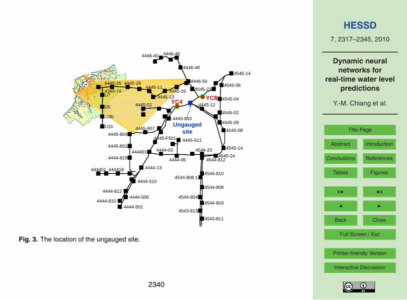
Moreover, in consideration of the historical inundation events recorded by the Hy-draulic Engineering Office of Taipei City Government, we selected an ungauged site,located between Stations YC4 and YC8, and marked it with a blue square as shown inFig. 3. In other words, this selected ungauged site is prone to inundation. Each numberdisplayed in Fig. 3 indicated a manhole related to a drain. Before the construction of a5

water level prediction model at an ungauged site, it should be confirmed if the qualityof the synthetic data of the water levels is appropriate or not. That is to say, the errorsmay propagate to the RNN if there are large biases in the synthetic data generated bythe SWMM. Hence, it is necessary to verify the applicability of a SWMM to the con-ditions of an urban sewerage system. In this research, the parameters of the SWMM10

were calibrated first on the historical gauge measurements basis. Then, the flows sim-ulated by the SWMM corresponding to Station YC4 and Station YC8 were evaluated.Figure 4a showed the rainfall hyetograph of an event randomly selected from datasets,whereas Fig. 4b and c showed the hydrographs of the SWMM output values versus theobservation values at Stations YC4 and YC8, accordingly. It clearly indicated that the15

water levels estimated by the SWMM well captured the main trends of observations atboth stations. The accuracies of the simulated flows at Stations YC4 and YC8 were0.96 and 0.98 each in terms of the correlation coefficient (CC). Results displayed inFig. 4 confirmed a high reliability of the SWMM simulations. Therefore, the SWMMis appropriate for generating the water level values at an ungauged site. Even if the20

SWMM is able to produce an accurate set of water level values, the outputs, however,are not predictions but simulations.

For predicting the water level at the selected ungauged site, the input variables ofa RNN consists of the precipitations and the water level information of the nearby up-stream and downstream stations; namely, the mean areal precipitations and water level25

observation values at Stations YC4 and YC8. It should be noticed that the learning tar-get values to the RNN is replaced by the synthetic data, assumed as the observationvalues, of water levels generated from the SWMM at the ungauged site. The RNNnetwork structure is expressed in Fig. 5. The best of this technique is this model can

2327





HESSD7, 2317–2345, 2010



Y.-M. Chiang et al.

Title Page



Tables Figures

J I

J I

Back Close

Full Screen / Esc



produce the water level predictions at any specific location no matter whether waterlevel measurements are available or not. It means this water level prediction modelcan be extended to any ungauged sites if the observation values of its nearby rainfallsand water levels are available. The RNN learned from both external, Stations YC4,YC8, and P, and internal, the feedback links, input information and further optimized its5

parameters in accordance with the errors calculated from related outputs and syntheticdata. The number of hidden neurons was set to three through trial-and-error proce-dures, and the training procedure has not been interrupted until the stop criterion wasreached.

Three error statistics are chosen to assess the consistency between the water level10

monitoring records and the RNN-based predictions; that is, the correlation coefficient(CC), coefficient of efficiency (CE), and normalized root-mean-square error (NRMSE).All of these indices are widely used to estimate the fitness to the hydrological mod-els in hydrological applications, and moreover to facilitate the comparison of differentestimated/predicted results. The three criteria are defined as follows:15

CC=

N∑i=1

(Q(i )−Q

)(Q̂(i )−Q̂

)√

N∑i=1

(Q(i )−Q

)2 N∑i=1

(Q̂(i )−Q̂

)2(5)

CE=1−

N∑i=1

(Q(i )−Q̂)2

N∑i=1

(Q(i )−Q)2

(6)

NRMSE=1σ

√√√√√ N∑i=1

(Q̂(i )−Q(i ))2

N(7)

2328





HESSD7, 2317–2345, 2010



Y.-M. Chiang et al.

Title Page



Tables Figures

J I

J I

Back Close

Full Screen / Esc



where Q̂ is the forecasted water level (m) and Q is the observed water level (m); Q and

Q̂ are the means of the water levels associated with observation values and forecastvalues, respectively. σ is the standard deviation of the observation values.

4 Results and discussion

4.1 Performance of water level predictions at the Gauging Station YC105

Table 2 shows the results obtained from the RNN for the water level predictions at Sta-tion YC10. The results implied that the model was well trained with a consistent perfor-mance and therefore produced precise testing results for multi-step-ahead forecasts.The testing performances of the water level predictions of 5-, 10-, 15-, and 20-min-ahead are rather good. We feel confident that the RNN-based water level prediction10

model is capable of capturing the major trends of observations with accuracy higherthan 0.97 of correlation coefficient, see Table 2. In terms of coefficient of efficiency(CE), the consistency between the water level observation values and the predictionvalues indicates that the RNN has the ability to predict highly nonlinear and variablesystems, such as urban drainage/sewerage systems. Figure 6 illustrates the scattering15

plots of the RNN outputs in both validation and testing sets versus the observationsfor 5 to 20-min-ahead predictions. The results clearly prove that the RNN can be welltrained for learning any input-output relations.

Figure 7 shows the error distribution of RNN outputs in testing phase for 5 to 20-min-ahead predictions. In the 5- and 10-min-ahead predictions of the model, the bi-20

ases between the outputs and observation values are mostly within 10 cm except forthe connection between a low water level event and a high level event with a slightunderestimation. A similar phenomenon also occurs in the 15- and 20-min-ahead pre-dictions since the water level measurements rise rapidly from 0.1 m to 1.27 m within20 min. However, there is no precipitation measured during this period. One possible25

2329





HESSD7, 2317–2345, 2010



Y.-M. Chiang et al.

Title Page



Tables Figures

J I

J I

Back Close

Full Screen / Esc



explanation may be the failure of hardware instruments. In summary, the RNN modelproved its ability to make precise predictions of 20-min-ahead water levels and per-formed well for peak flow predictions.

4.2 Performance of water level predictions at an ungauged site

As mentioned previously, there is a need for building the water level prediction at an5

ungauged site since monitoring the water levels in urban sewerage systems is not yetvery common in Taiwan. In order to conquer the difficulty in predicting the water levelat an ungauged site, we utilized the precipitation and the water level information ofthe nearby stations as input and the synthetic data obtained form the SWMM as thetarget values, because of the unavailability of real observation values at this site, to10

train the RNN. Table 3 shows the testing results calculated by all criteria at the chosenungauged site. For 5- to 20-min-ahead predictions, the values of CC are higher than0.95, indicating that the RNN can effectively predict the water level hydrographs evenat an ungauged site. Nevertheless, values of CE, falling between 0.74 and 0.83, arerelatively low which implies that the RNN slightly underestimated some peak flows with15

an error percentage under 10%. Figure 8 illustrates the scattering plots of the RNNoutputs versus the SWMM estimations. For the 5-min-ahead prediction, refer to Fig. 8a,the prediction values are very close to the ideal line which indicates a high accuracyof the RNN outputs. In the analysis of the 10- to 20-min-ahead prediction values, seeFig. 8b–d, it is quite obvious that the RNN underestimates some observation values.20

The major reason for producing such underestimation is due to the time-lag problemswhich occur in the output process of the RNN. Fortunately, the phenomenon of suchunderestimation is not that serious. In summary, the results obtained from RNN are stillacceptable, indicating that the RNN is also applicable to the water level predictions atungauged sites by using synthetic data sets generated from a well calibrated SWMM.25

Overall, the study demonstrates that the RNN model is capable of learning the time-varying processes in urban sewerage systems, and therefore providing precise waterlevel predictions up to 20-min-ahead. It is interesting to inspect the model performance

2330





HESSD7, 2317–2345, 2010



Y.-M. Chiang et al.

Title Page



Tables Figures

J I

J I

Back Close

Full Screen / Esc



at gauged and ungauged sites. For example, the RNN models produced smaller pre-dictive error at gauged site but larger predictive error at ungauged site (in terms ofCE and NRMSE) even though the correlation coefficients at both sites are higher than0.95. This is because the hydrograph of the synthetic data generated by SWMM is notas smooth as that of observations (see Fig. 4). In other words, the bias produced from5

synthetic data does propagate to RNN model, and therefore resulted in larger predic-tive error. Besides, the correlation coefficients of the SWMM simulations achieved 0.96and 0.98 at YC4 and YC8, respectively, which indicates the best performance obtainedat ungauged site will not be higher than 0.98. Our results conform to this limitation (seeTable 3) and demonstrate that the predictive capabilities of RNN models are similar no10

matter where it is.

5 Conclusions

In this research, the recurrent-neural-network-based hydrological models have beendeveloped to predict the water levels at both gauged and ungauged sites. This tech-nique was applied to a sewerage system in the biggest urbanized catchment in Taipei15

City. Eight RNN models (four for YC10 gauged site, and four for ungauged site), eachwith a single output, were calibrated by using the mean areal precipitations and up-stream hydrological information, and then built for the multi-step-ahead water level pre-dictions. The related outputs can provide important prior knowledge and/or informationfor the successful operation of pumping stations in an urban sewerage system, and the20

accurate water level predictions should offer an improvement in preventing a city frominundation.

The RNN-based hydrological models can precisely estimate the observation valuesat the catchment outlet. For the prediction at the gauged site, Station YC10, the RNNproduced excellent water level outputs for 5- up to 20-min-ahead predictions. As far as25

the statistical criteria are concerned, the values of both CC and CE are higher than 0.97in testing phase, indicating that the RNN is very suitable to model the nonlinear and

2331





HESSD7, 2317–2345, 2010



Y.-M. Chiang et al.

Title Page



Tables Figures

J I

J I

Back Close

Full Screen / Esc



time-varying mechanisms of an urban sewerage system. For the prediction at the un-gauged site, the SWMM was used for computing storm sewer flow and generating dataat the selected manhole. Based on the evaluation of the SWMM’s applicability to anurban sewerage system, the synthetic data at an ungauged manhole were generatedfor the training of the RNN. These results pointed out that even though the forecasts of5

the RNN slightly underestimated the peak flows, the RNN model effectively capturedthe major trends of the water level hydrographs produced by the SWMM. We are cer-tain that this proposed method can be used in a more flexible way for constructing thehydrological prediction model at any specific manhole. Likewise, the results can beof great help to verify the inundation risk and to enhance the efficiency of a pumping10

station in an inundation-prone area if a suitable operational strategy can be made.

Acknowledgements. This research was sponsored by the Water Resource Agency, Taiwan,R.O.C. The Taipei City Government provided the sewerage gauging data for analysis purposein this research.

References15

Ackerman, D. and Schiff, K.: Modeling storm water mass emissions to the southern Californiabight, J. Environ. Eng.-Asce, 129(4), 308–317, 2003.

Akhtar, M. K., Corzo, G. A., van Andel, S. J., and Jonoski, A.: River flow forecasting withartificial neural networks using satellite observed precipitation pre-processed with flow lengthand travel time information: case study of the Ganges river basin, Hydrol. Earth Syst. Sci.,20

13, 1607–1618, 2009,http://www.hydrol-earth-syst-sci.net/13/1607/2009/.

Baffaut, C. and Delleur, J. W.: Calibration of Swmm Runoff Quality Model with Expert System,J. Water Res. Pl.-Asce, 116(2), 247–261, 1990.

Borah, D. K. and Bera, M.: Watershed-scale hydrologic and nonpoint-source pollution models:25

Review of mathematical bases, T. Asae, 46(6), 1553–1566, 2003.Bruen, M. and Yang, J. Q.: Combined hydraulic and black-box models for flood forecasting in

urban drainage systems, J. Hydrol. Eng., 11(6), 589–596, 2006.

2332





http://www.hydrol-earth-syst-sci.net/13/1607/2009/

HESSD7, 2317–2345, 2010



Y.-M. Chiang et al.

Title Page



Tables Figures

J I

J I

Back Close

Full Screen / Esc



Chandramouli, V. and Deka, P.: Neural network based decision support model for optimalreservoir operation, Water Resour. Manag., 19(4), 447–464, 2005.

Chang, F. J., Chang, L. C. and Huang, H. L.: Real-time recurrent learning neural network forstream-flow forecasting, Hydrol. Process., 16(13), 2577–2588, 2002.

Chang, F. J. and Chang, Y. T.: Adaptive neuro-fuzzy inference system for prediction of water5

level in reservoir, Adv. Water Resour., 29(1), 1–10, 2006.Chang, L. C. and Chang, F. J.: Intelligent control for modelling of real-time reservoir operation,

Hydrol. Process., 15(9), 1621–1634, 2001.Chaves, P. and Chang, F. J.: Intelligent reservoir operation system based on evolving artificial

neural networks, Adv. Water Resour., 31(6), 926–936, 2008.10

Chiang, Y. M. and Chang, F. J.: Integrating hydrometeorological information for rainfall-runoffmodelling by artificial neural networks, Hydrol. Process., 23(11), 1650–1659, 2009.

Chiang, Y. M., Chang, F. J., Jou, B. J. D., and Lin, P. F.: Dynamic ANN for precipitation estimationand forecasting from radar observations, J. Hydrol., 334(1–2), 250–261, 2007a.

Chiang, Y. M., Chang, L. C., and Chang, F. J.: Comparison of static-feedforward and dynamic-15

feedback neural networks for rainfall-runoff modeling, J. Hydrol., 290(3–4), 297–311, 2004.Chiang, Y. M., Hsu, K. L., Chang, F. J., Hong, Y., and Sorooshian, S.: Merging multiple precipi-

tation sources for flash flood forecasting, J. Hydrol., 340(3–4), 183–196, 2007b.Coulibaly, P. and Baldwin, C. K.: Nonstationary hydrological time series forecasting using non-

linear dynamic methods, J. Hydrol., 307(1–4), 164–174, 2005.20

Coulibaly, P. and Evora, N. D.: Comparison of neural network methods for infilling missing dailyweather records, J. Hydrol., 341(1–2), 27–41, 2007.

Denault, C., Millar, R. G., and Lence, B. J.: Assessment of possible impacts of climate changein an urban catchment, J. Am. Water Resour. As., 42(3), 685–697, 2006.

Huber, W. C. and Dickinson, R. E.: Strom water management model. User’s Manual Ver. IV, US25

Environmental Protection Agency, 1988.Hung, N. Q., Babel, M. S., Weesakul, S., and Tripathi, N. K.: An artificial neural network model

for rainfall forecasting in Bangkok, Thailand, Hydrol. Earth Syst. Sci., 13, 1413–1425, 2009,http://www.hydrol-earth-syst-sci.net/13/1413/2009/.

Kumar, D. N., Raju, K. S., and Sathish, T.: River flow forecasting using recurrent neural net-30

works, Water Resour. Manag., 18(2), 143–161, 2004.Loke, E., Warnaars, E. A., Jacobsen, P., Nelen, F., and Almeida, M. D.: Artificial neural networks

as a tool in urban storm drainage, Water Sci. Technol., 36(8–9), 101–109, 1997.

2333






HESSD7, 2317–2345, 2010



Y.-M. Chiang et al.

Title Page



Tables Figures

J I

J I

Back Close

Full Screen / Esc



Maharjan, M., Pathirana, A., Gersonius, B., and Vairavamoorthy, K.: Staged cost optimization ofurban storm drainage systems based on hydraulic performance in a changing environment,Hydrol. Earth Syst. Sci., 13, 481–489, 2009,http://www.hydrol-earth-syst-sci.net/13/481/2009/.

Maity, R. and Kumar, D. N.: Basin-scale stream-flow forecasting using the information of large-5

scale atmospheric circulation phenomena, Hydrol. Process., 22(5), 643–650, 2008.Mishra, A. K. and Desai, V. R.: Drought forecasting using feed-forward recursive neural net-

work, Ecol. Model., 198(1–2), 127–138, 2006.Nasseri, M., Asghari, K., and Abedini, M. J.: Optimized scenario for rainfall forecasting using

genetic algorithm coupled with artificial neural network, Expert Syst. Appl., 35(3), 1415–10

1421, 2008.Razavi, S. and Karamouz, M.: Adaptive neural networks for flood routing in river systems,

Water Int., 32(3), 360–375, 2007.Sudheer, K. P., Srinivasan, K., Neelakantan, T. R., and Srinivas, V. V.: A nonlinear data-driven

model for synthetic generation of annual streamflows, Hydrol. Process., 22(12), 1831–1845,15

2008.Toth, E.: Classification of hydro-meteorological conditions and multiple artificial neural networks

for streamflow forecasting, Hydrol. Earth Syst. Sci., 13, 1555–1566, 2009,http://www.hydrol-earth-syst-sci.net/13/1555/2009/.

Tsihrintzis, V. A. and Hamid, R.: Runoff quality prediction from small urban catchments using20

SWMM, Hydrol. Process., 12(2), 311–329, 1998.Yazdani, M. R., Saghafian, B., Mahdian, M. H., and Soltani, S.: Monthly Runoff Estimation

Using Artificial Neural Networks, J. Agric. Sci. Technol., 11(3), 355–362, 2009.

2334







HESSD7, 2317–2345, 2010



Y.-M. Chiang et al.

Title Page



Tables Figures

J I

J I

Back Close

Full Screen / Esc



Table 1. Data from storm events for water level predictions.

Configuration Event Amount Rainfall Mean water Standardaccumulation level deviation

(mm) (m) (m)

1

Training

395 90.8 2.10 0.612 85 20.9 2.25 0.333 68 15.0 2.28 0.264 107 33.0 1.44 0.575 31 68.4 1.84 0.276 256 406.5 5.48 1.267 206 156.4 3.20 0.388 300 156.1 2.63 0.74

9

Validation

135 123.0 2.32 0.8310 60 61.8 1.77 0.6211 43 21.0 1.33 0.15

12

Testing

142 53.2 2.06 0.6513 176 57.2 2.04 0.5514 51 25.3 1.46 0.65

2335





HESSD7, 2317–2345, 2010



Y.-M. Chiang et al.

Title Page



Tables Figures

J I

J I

Back Close

Full Screen / Esc



Table 2. Results obtained from the RNN for water level prediction at Station YC10.

Index Lead time

5 min 10 min 15 min 20 min

CC 0.99 0.99 0.99 0.99Training CE 0.99 0.99 0.98 0.97

NRMSE 0.08 0.08 0.15 0.16

CC 0.99 0.99 0.97 0.97Validation CE 0.99 0.98 0.95 0.93

NRMSE 0.12 0.16 0.23 0.26

CC 0.99 0.99 0.97 0.97Testing CE 0.99 0.99 0.97 0.95

NRMSE 0.11 0.11 0.22 0.26

2336





HESSD7, 2317–2345, 2010



Y.-M. Chiang et al.

Title Page



Tables Figures

J I

J I

Back Close

Full Screen / Esc



Table 3. Testing results of the water level prediction at an ungauged site.

CC CE NRMSE

5-min-ahead 0.98 0.83 0.3610-min-ahead 0.97 0.82 0.4215-min-ahead 0.97 0.76 0.4320-min-ahead 0.95 0.74 0.44

2337





HESSD7, 2317–2345, 2010



Y.-M. Chiang et al.

Title Page



Tables Figures

J I

J I

Back Close

Full Screen / Esc



11 JJ

11

II11

DD11

DDJJ…

KK

…

…

…Inputlayer

Hiddenlayer

Outputlayer

Time-delayunits

22

22

DD22

Input variables

Outputs

DD11

DDKK

…

545

Figure 1 The architecture of the recurrent neural network (RNN) 546

547

Fig. 1. The architecture of the recurrent neural network (RNN).

2338





HESSD7, 2317–2345, 2010



Y.-M. Chiang et al.

Title Page



Tables Figures

J I

J I

Back Close

Full Screen / Esc



548

549

Figure 2 The locations of Yu-Cheng catchment and the monitoring stations 550

551

Fig. 2. The locations of Yu-Cheng catchment and the monitoring stations.

2339





HESSD7, 2317–2345, 2010



Y.-M. Chiang et al.

Title Page



Tables Figures

J I

J I

Back Close

Full Screen / Esc



552

4545-14

4545-06

4545-04

4545-02

4545-09

4545-08

4545-14

4545-24

4544-810

4544-808

4544-803

4543-811

4544-804

4543-813

4544-808.1

4544-812

4544-20

4444-06

4445-511

4444-03

4444-13

4444-819

4445-801

4445-8044445-907

4444-510

4444-506

4444-5014444-810

4444-812

444418444451

444401

4445-F501

4445-810

4445-02 4445-12

4545-23

4446-50

4446-48

4446-464446-40

4445-164445-13

4445-114445-284445-25

4345-74U7

U5

U3b

U1b

YC4 YC8

Ungaugedsite

553

Figure 3 The location of the ungauged site 554

555

Fig. 3. The location of the ungauged site.

2340





HESSD7, 2317–2345, 2010



Y.-M. Chiang et al.

Title Page



Tables Figures

J I

J I

Back Close

Full Screen / Esc



0 50 100 150 2000

2

4

6

8

0 50 100 150 2000

2

4

6

8

0 50 100 150 2001

1.5

2

2.5

3

3.5

4

4.5

玉成4 obs

玉成4 swmmObs.SWMM

0 50 100 150 2001

1.5

2

2.5

3

3.5

4

4.5

玉成4 obs


0 50 100 150 2001

1.5

2

2.5

3

3.5

4

4.5

玉成8 obs


0 50 100 150 2001

1.5

2

2.5

3

3.5

4

4.5

玉成8 obs


CC=0.96

CC=0.98

Leve

l (m

)

Lev

el (m

)

prec

ipita

tion

(mm

)

(a)

(b)

(c)Time (5-min)

556

Figure 4 (a) The rainfall hyetograph, (b) the SWMM hydrograph at Station YC4, (c) 557 the SWMM hydrograph at Station YC8 558

Fig. 4. (a) The rainfall hyetograph, (b) the SWMM hydrograph at Station YC4, (c) the SWMMhydrograph at Station YC8.

2341





HESSD7, 2317–2345, 2010



Y.-M. Chiang et al.

Title Page



Tables Figures

J I

J I

Back Close

Full Screen / Esc



559

Optimization

Synthetic dataset

YC4

YC8

P

Parameters calibration

PredictionE

EvaluationSynthetic dataset

EXTRANRUNOFF

Time-delay unit

560

Figure 5 The architecture of a RNN to predict the water level at the ungauged station 561 Fig. 5. The architecture of a RNN to predict the water level at the ungauged station.

2342





HESSD7, 2317–2345, 2010



Y.-M. Chiang et al.

Title Page



Tables Figures

J I

J I

Back Close

Full Screen / Esc



(a)

562

(a)

-1 0 1 2 3-1

0

1

2

3

observation(m)

pre

dic

tion

(m)

Validation

-1 0 1 2 3-1

0

1

2

3

observation(m)

pre

dic

tion

(m)

Testing

(b)

-1 0 1 2 3-1

0

1

2

3

observation(m)

pre

dic

tion

(m)

Validation

-1 0 1 2 3-1

0

1

2

3

observation(m)

pre

dic

tion

(m)

Testing

(c)

-1 0 1 2 3-1

0

1

2

3

observation(m)

pre

dic

tion

(m)

Validation

-1 0 1 2 3-1

0

1

2

3

observation(m)

pre

dic

tion

(m)

Testing

(d)

-1 0 1 2 3-1

0

1

2

3

observation(m)

pre

dic

tion

(m)

Validation

-1 0 1 2 3-1

0

1

2

3

observation(m)

pre

dic

tion

(m)

Testing

Figure 6 The scattering plots of the RNN outputs versus the observations for (a) 5-, 563 (b) 10-, (c) 15-, and (d) 20-minute-ahead predictions in both validation and 564

testing sets 565

(b)

562

(a)

-1 0 1 2 3-1

0

1

2

3

observation(m)

pre

dic

tion

(m)

Validation

-1 0 1 2 3-1

0

1

2

3

observation(m)

pre

dic

tion

(m)

Testing

(b)

-1 0 1 2 3-1

0

1

2

3

observation(m)

pre

dic

tion

(m)

Validation

-1 0 1 2 3-1

0

1

2

3

observation(m)

pre

dic

tion

(m)

Testing

(c)

-1 0 1 2 3-1

0

1

2

3

observation(m)

pre

dic

tion

(m)

Validation

-1 0 1 2 3-1

0

1

2

3

observation(m)

pre

dic

tion

(m)

Testing

(d)

-1 0 1 2 3-1

0

1

2

3

observation(m)

pre

dic

tion

(m)

Validation

-1 0 1 2 3-1

0

1

2

3

observation(m)

pre

dic

tion

(m)

Testing


testing sets 565

(c)

562

(a)

-1 0 1 2 3-1

0

1

2

3

observation(m)

pre

dic

tion

(m)

Validation

-1 0 1 2 3-1

0

1

2

3

observation(m)

pre

dic

tion

(m)

Testing

(b)

-1 0 1 2 3-1

0

1

2

3

observation(m)

pre

dic

tion

(m)

Validation

-1 0 1 2 3-1

0

1

2

3

observation(m)

pre

dic

tion

(m)

Testing

(c)

-1 0 1 2 3-1

0

1

2

3

observation(m)

pre

dic

tion

(m)

Validation

-1 0 1 2 3-1

0

1

2

3

observation(m)

pre

dic

tion

(m)

Testing

(d)

-1 0 1 2 3-1

0

1

2

3

observation(m)

pre

dic

tion

(m)

Validation

-1 0 1 2 3-1

0

1

2

3

observation(m)

pre

dic

tion

(m)

Testing


testing sets 565

(d)

562

(a)

-1 0 1 2 3-1

0

1

2

3

observation(m)

pre

dic

tion

(m)

Validation

-1 0 1 2 3-1

0

1

2

3

observation(m)

pre

dic

tion

(m)

Testing

(b)

-1 0 1 2 3-1

0

1

2

3

observation(m)

pre

dic

tion

(m)

Validation

-1 0 1 2 3-1

0

1

2

3

observation(m)

pre

dic

tion

(m)

Testing

(c)

-1 0 1 2 3-1

0

1

2

3

observation(m)

pre

dic

tion

(m)

Validation

-1 0 1 2 3-1

0

1

2

3

observation(m)

pre

dic

tion

(m)

Testing

(d)

-1 0 1 2 3-1

0

1

2

3

observation(m)

pre

dic

tion

(m)

Validation

-1 0 1 2 3-1

0

1

2

3

observation(m)

pre

dic

tion

(m)

Testing


testing sets 565 Fig. 6. The scattering plots of the RNN outputs versus the observations for (a) 5-, (b) 10-, (c) 15-, and (d) 20-min-ahead predictions in both validation and testing sets.

2343





HESSD7, 2317–2345, 2010



Y.-M. Chiang et al.

Title Page



Tables Figures

J I

J I

Back Close

Full Screen / Esc



(a)-0.7 -0.6 -0.5 -0.4 -0.3 -0.2 -0.1 0 0.1 0.2 0.30

20

40

60

bias(m)(f

req.

)

(a)

-0.6 -0.5 -0.4 -0.3 -0.2 -0.1 0 0.1 0.2 0.30

20

40

60

bias(m)

(fre

q.)

(b)

-1 -0.8 -0.6 -0.4 -0.2 0 0.2 0.40

20

40

60

bias(m)

(fre

q.)

(c)

-1.2 -1 -0.8 -0.6 -0.4 -0.2 0 0.2 0.4 0.60

20

40

60

bias(m)

(fre

q.)

(d)

Figure 7 The error distribution of RNN outputs in testing phase for (a) 5-, (b) 10-, (c) 566 15-, and (d) 20-minute-ahead predictions 567

568

(b)

-0.7 -0.6 -0.5 -0.4 -0.3 -0.2 -0.1 0 0.1 0.2 0.30

20

40

60

bias(m)

(fre

q.)

(a)

-0.6 -0.5 -0.4 -0.3 -0.2 -0.1 0 0.1 0.2 0.30

20

40

60

bias(m)

(fre

q.)

(b)

-1 -0.8 -0.6 -0.4 -0.2 0 0.2 0.40

20

40

60

bias(m)

(fre

q.)

(c)

-1.2 -1 -0.8 -0.6 -0.4 -0.2 0 0.2 0.4 0.60

20

40

60

bias(m)

(fre

q.)

(d)


568

(c)

-0.7 -0.6 -0.5 -0.4 -0.3 -0.2 -0.1 0 0.1 0.2 0.30

20

40

60

bias(m)

(fre

q.)

(a)

-0.6 -0.5 -0.4 -0.3 -0.2 -0.1 0 0.1 0.2 0.30

20

40

60

bias(m)

(fre

q.)

(b)

-1 -0.8 -0.6 -0.4 -0.2 0 0.2 0.40

20

40

60

bias(m)

(fre

q.)

(c)

-1.2 -1 -0.8 -0.6 -0.4 -0.2 0 0.2 0.4 0.60

20

40

60

bias(m)

(fre

q.)

(d)


568

(d)

-0.7 -0.6 -0.5 -0.4 -0.3 -0.2 -0.1 0 0.1 0.2 0.30

20

40

60

bias(m)

(fre

q.)

(a)

-0.6 -0.5 -0.4 -0.3 -0.2 -0.1 0 0.1 0.2 0.30

20

40

60

bias(m)

(fre

q.)

(b)

-1 -0.8 -0.6 -0.4 -0.2 0 0.2 0.40

20

40

60

bias(m)

(fre

q.)

(c)

-1.2 -1 -0.8 -0.6 -0.4 -0.2 0 0.2 0.4 0.60

20

40

60

bias(m)

(fre

q.)

(d)


568

Fig. 7. The error distribution of RNN outputs in testing phase for (a) 5-, (b) 10-, (c) 15-, and(d) 20-min-ahead predictions.

2344





HESSD7, 2317–2345, 2010



Y.-M. Chiang et al.

Title Page



Tables Figures

J I

J I

Back Close

Full Screen / Esc



(a)0 1 2 3 4

0

1

2

3

4

SWMM (m)

RN

N (

m)

0 1 2 3 40

1

2

3

4

SWMM (m)

RN

N (

m)

(a) (b)

0 1 2 3 40

1

2

3

4

SWMM (m)

RN

N (

m)

0 1 2 3 40

1

2

3

4

SWMM (m)

RN

N (

m)

(c) (d)

Figure 8 The scattering plots of the RNN outputs versus the SWMM estimations for 569 (a) 5-, (b) 10-, (c) 15-, and (d) 20-minute-ahead predictions in testing set 570

571

(b)0 1 2 3 4

0

1

2

3

4

SWMM (m)

RN

N (

m)

0 1 2 3 40

1

2

3

4

SWMM (m)

RN

N (

m)

(a) (b)

0 1 2 3 40

1

2

3

4

SWMM (m)

RN

N (

m)

0 1 2 3 40

1

2

3

4

SWMM (m)

RN

N (

m)

(c) (d)


571

(c)

0 1 2 3 40

1

2

3

4

SWMM (m)

RN

N (

m)

0 1 2 3 40

1

2

3

4

SWMM (m)

RN

N (

m)

(a) (b)

0 1 2 3 40

1

2

3

4

SWMM (m)

RN

N (

m)

0 1 2 3 40

1

2

3

4

SWMM (m)

RN

N (

m)

(c) (d)


571

(d)

0 1 2 3 40

1

2

3

4

SWMM (m)

RN

N (

m)

0 1 2 3 40

1

2

3

4

SWMM (m)

RN

N (

m)

(a) (b)

0 1 2 3 40

1

2

3

4

SWMM (m)

RN

N (

m)

0 1 2 3 40

1

2

3

4

SWMM (m)

RN

N (

m)

(c) (d)


571

Fig. 8. The scattering plots of the RNN outputs versus the SWMM estimations for (a) 5-,(b) 10-, (c) 15-, and (d) 20-min-ahead predictions in testing set.

2345





dynamic neural networks for real-time water level predictions

Documents