training dynamic neural networks for forecasting naira...

American Journal of Management Science and Engineering 2016; 1(1): 8-14

http://www.sciencepublishinggroup.com/j/ajmse

doi: 10.11648/j.ajmse.20160101.12

Training Dynamic Neural Networks for Forecasting Naira/Dollar Exchange Returns Volatility in Nigeria

S. Suleiman1, S. U. Gulumbe

1, B. K. Asare

1, M. Abubakar

2

1Department of Mathematics, Usmanu Danfodiyo University, Sokoto, Nigeria 2Department of Economics, Usmanu Danfodiyo University, Sokoto, Nigeria

Email address:

[email protected] (S. Suleiman), [email protected] (S. Suleiman)

To cite this article: S. Suleiman, S. U. Gulumbe, B. K. Asare, M. Abubakar. Training Dynamic Neural Networks for Forecasting Naira/Dollar Exchange Returns

Volatility in Nigeria. American Journal of Management Science and Engineering. Vol. 1, No. 1, 2016, pp. 8-14.

doi: 10.11648/j.ajmse.20160101.12

Received: August 13, 2016; Accepted: August 22, 2016; Published: September 9, 2016

Abstract: This paper examined the monthly volatility of Naira/Dollar exchange rates in Nigeria between the periods of

January, 1995 to January, 2016. Forecasting volatility remains to be an important step to be taken in several decision makings

involving financial market. Traditional GARH models were usually applied in forecasting volatility of a financial market. This

study was aim at enhancing the performance of these models in volatility forecasting in which both the traditional GARCH and

Dynamic Neural Networks were hybridized to develop the proposed models offorecasting the volatility of Inflation rate in

Nigeria. The values of the volatility estimated by the best fitted GARH model are used as input to the Neural Network. The

inputs of the first hybrid model also included past values of other related endogenous variables. The second hybrid model takes

as inputs both series of the simulated data and the inputs of the first hybrid model. The forecasts obtained by each of those

hybrid models have been compared with those of GARCH model in terms of the actual volatility. The computational results

demonstrate that the second hybrid model provides better volatility forecasts.

Keywords: Volatility, ARCH Models, Dynamic Neural Networks, Monthly Standard Deviation

1. Introduction

Before the establishment of structural adjustment

programme in Nigeria in 1986, there was a fixed exchange

rate in the country which was maintained by the exchange

control regulations that brought about significant distortions

in the economy. This is because Nigeria depends seriously on

imports from different countries as nearly all industries

import their raw materials from foreign countries. Similarly,

there were huge importation of finished goods with the

adverse consequences for domestic production, balance of

payments position and the nation’s external reserves level

[1]. The foreign exchange market in the fixed exchange rate

period was characterized by high demand for foreign

exchange which cannot be adequately met with the supply of

foreign exchange by the Central Bank of Nigeria (CBN). The

fixed exchange rate period was also characterized by sharp

practices perpetrated by dealers and end-users of foreign

exchange [1]. The inadequate supply of foreign exchange by

the CBN promoted the parallel market for foreign exchange

and created uncertainty in foreign exchange rates. The

introduction of SAP in Nigeria in September 1986 which

deregulated the foreign exchange market led to the

introduction of market determined exchange rate, managed

floating rate regime. The CBN usually intervene in foreign

exchange market through its monetary policy actions and

operations in the money market to influence the exchange

rate movement in the desired direction such that it ensures

the competitiveness of the domestic economy. This

introduction of managed floating rate regime tends to

increase the uncertainty in exchange rates, thus, increasing

the volatility of exchange rate by the regime shifts. This

made the exchange rate to be the most important asset price

in the economy.

The volatility of time series as defined by econometricians

refer to the ‘conditional variance’ of the data and the time-

varying volatility typical of asset return which is otherwise

known as ‘conditional heteroscedasticity’. The conditional

heteroscedasticity was a theory first introduced to economists

by [2] in which conditional variance of a time series is

American Journal of Management Science and Engineering 2016; 1(1): 8-14 9

considered as a function of past shocks; the autoregressive

conditional heteroscedastic (ARCH) model. The model

provided a precise approach of empirically investigating

issues concerning the volatility of economic variables. An

example is Friedman's hypothesis that higher inflation is

more volatile [3]. Using data for the UK, Engle [2] found that

the ARCH model supported Friedman's hypothesis. [4]

Applied the ARCH model to US inflation and the converse

results emerged, although [5] criticize this paper as they

believe that Engle estimates a mis-specified model. The

relationship between the level and variance of inflation has

continued to interest applied econometricians [6].

Artificial Neural Network (ANN) gives a better way of

investigating the dynamics of different problems pertaining

to Economics and Finance [7]. The use of these techniques to

economic application is growing fast [8, 9, 10, 11]. [12]

Improved traditional GARCH models with the use of ANN in

which they forecast the volatility of daily return of Istanbul

Stock Exchange. [13] Used three hybridized time series with

ANN models in order to forecast the volatility of Korea

Composite Stock Price Index (KOSPI 200). Traditional

GARCH models are mostly used in forecasting and

simulation of a financial variable. The ability of model

toforecast volatility very well indicates the power of that

model because volatility is central to several decisions in

financial markets. The aim of this study is to integrate

dynamic neural networks in to traditional GARCH models in

the forecast volatility of Naira/Dollar Exchange ratein

Nigeria.

2. GARCH Models

The unpredictable manners in financial markets is known

as the ‘‘volatility’’. Volatility has turn into a central theory in

diverse areas of financial engineering, such as multi-period

portfolio selection, risk management, and derivative pricing

[7]. Volatility estimates is also being utilized by various asset

pricing models as a simple risk measure. It is as well

considered as an important contribution to the well-known

Black–Sholes model for option pricing with its many

branches. In statistics, volatility is commonly calculated by

standard deviation or variance [14]. In recent times, different

models which used stochastic volatility process and time

series modeling were used in place of implied and historical

volatility method. [2] Developed and used ARCH model to

estimate volatility and his original work on ARCH was

extended in GARCH [15], EGARCH [16] and GJR-GARCH

[17]. Generalized Autoregressive Conditional

Heteroscedasticity, GARCH (p, q) makes the current

conditional variance to depend on the p past conditional

variances and the q past squared innovations. The GARCH

(p, q) model can be expressed as:

�� = �� (1)

�� = � + ∑ �� + ∑ �� (2)

�, �, �� are non-negativeparameters to be estimated, �� is

anindependently and identically distributed (i.i.d.) random

variables with zero mean and unit variance and �� is a serially

uncorrelated sequence with zero mean and the conditional

variance of �� which may be nonstationary, the GARCH

model reduces the number of parameters necessary when

information in the lag(s) of the conditional variance in

addition to the lagged �� terms were considered, but was

not able to account for asymmetric behavior of the returns.

[16] establish Exponential Generalized Autoregressive

Conditional Heteroscedasticity (EGARCH) model in order to

capture leverage effects of price change on conditional

variance and which can be written as follows:

�� = � + � � ��

− � ��

��

��

+ ∑ �� + ∑ ��(!"#$

%"#$)'�� (3)

The parameters � and �� in equation (3) were not

constrained in order to guarantee positive and zero

conditional variances. GJR-GARCH is another model which

used to measure the asymmetric features of the returns series

and it is very similar to the Threshold GARCH (TGARCH),

and Asymmetric GARCH (AGARCH) due to [18] and [19]

respectively. The GJR (p, q) can be written as:

�� = � + ∑ �� + ∑ [��)(�� < 0)�� ] + ∑ �� (4)

Where ��(- = 1, … , 0) are the asymmetric parameter and

)(. ) is the indicator function defined such that )((�� <0) = 1 if �� < 0 and )((�� > 0) = 0 if�� > 0

Equally, asymmetric ARCH known as APARCH (p, q) was

introduced by [20] and is represented as:

��3 = � + ∑ �(|��| − ��)3 + �� ∑ ��3�� (5)

where the asymmetric parameter −1 < �� < 1(- = 1 … , 0), with non-negative 5 transforms the conditional standard

deviation and asymmetric absolute innovations.

3. Dynamic Neural Networks

Neural networks can be classified into dynamic and static

categories. Static (feed forward) networks have no feedback

elements and contain no delays; the output is calculated

directly from the input through feed forward connections. In

dynamic networks (such as Non-linear Auto-Regressive

model with exogenous inputs (NARX), the output depends

not only on the current input to the network, but also on the

current or previous inputs, outputs, or states of the network.

Dynamic networks are generally more powerful than static

networks (although somewhat more difficult to train).

Because dynamic networks have memory, they can be trained

to learn sequential or time-varying patterns. This has

applications in such disparate areas as prediction in financial

markets [21], channel equalization in communication

systems [22], phase detection in power systems [23] and

many more dynamic network applications in [24].

10 S. Suleiman et al.: Training Dynamic Neural Networks for Forecasting Naira/Dollar

Exchange Returns Volatility in Nigeria

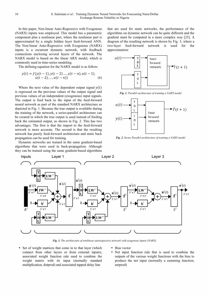
In this paper, Non-linear Auto-Regressive with Exogenous

(NARX) inputs was employed. This model has a parametric

component plus a nonlinear part, where the nonlinear part is

approximated by a single hidden layer feed-forward ANN.

The Non-linear Auto-Regressive with Exogenous (NARX)

inputs is a recurrent dynamic network, with feedback

connections enclosing several layers of the network. The

NARX model is based on the linear ARX model, which is

commonly used in time-series modeling.

The defining equation for the NARX model is as follow:

6(7) = 8(6(7 − 1&, 6 7 � 2& … , 6 7 � :&, ; 7 � 1&, ; 7 � 2&, … , ; 7 � :&& (6)

Where the next value of the dependent output signal 6 7&

is regressed on the previous values of the output signal and

previous values of an independent (exogenous) input signals.

The output is feed back to the input of the feed-forward

neural network as part of the standard NARX architecture as

depicted in Fig. 1. Because the true output is available during

the training of the network, a series-parallel architecture can

be created in which the true output is used instead of feeding

back the estimated output, as shown in Fig. 2. This has two

advantages. The first is that the import to the feed-forward

network is more accurate. The second is that the resulting

network has purely feed-forward architecture and static back

propagation can be used for training.

Dynamic networks are trained in the same gradient-based

algorithms that were used in back-propagation. Although

they can be trained using the same gradient-based algorithms

that are used for static networks, the performance of the

algorithms on dynamic network can be quite different and the

gradient must be computed in a more complex way [25]. A

diagram of the resulting network is shown by Fig. 3, where a

two-layer feed-forward network is used for the

approximation:

Fig. 1. Parallel architecture of training a NARX model.

Fig. 2. Series Parallel architecture of training a NARX model.

Fig. 3. The architecture of nonlinear autoregressive network with exogenous inputs (NARX).

� Set of weight matrices that come in to that layer (which

connect from other layers or from external inputs),

associated weight function rule used to combine the

weight matrix with its input (normally standard

multiplication, dotprod) and associated tapped delay line

� Bias vector

� Net input function rule that is used to combine the

outputs of the various weight functions with the bias to

produce the net input (normally a summing function,

netprod)


� Transfer function

The network has inputs that are connected to special

weights, called input weights and denoted by <=�,�, where >

denotes the number of the input vector that enters the weight

and - denotes the number of the layer to which the weight is

connected. The weights connecting one layer to another are

called layer weights and are denoted by ?=�,� , where >

denotes the number of the layer coming in to the weight and - denotes the number of the layer at the output of the weight.

This type of network’s weights has two different effects on

the network output. The first is the direct effect, because a

change in the weight causes an immediate change in the

output at the current time step (this first effect can be

computed using standard back propagation). The second is an

indirect effect, because some of the inputs to the layer, such

as (7, 1&, are also functions of the weights. To account for this

indirect effect, the dynamic back propagation must be used to

compute the gradients, which are more computationally

intensive [25]. Expect dynamic back propagation to take

more time to train, in part for this reason. In addition, the

error surfaces for dynamic networks can be more complex

than those for static networks. Training is more likely to be

trapped in local minima. This suggests that that you might

need to train the network several times to achieve an optimal

result [26].

4. Artificial Neural Network-Based

Methodology

The nonlinear autoregressive network with exogenous

inputs is used to forecast the closing price returns of the

Naira/Dollar exchange rate in the following.

It is assumed that @� is the closing returns value at the

moment of time 7. For each time 7, there is a vector A� � A� �&, A� �&, … , A� B&&C whose entries are the values of the

indicators significantly correlated to @�, that is the correlation

coefficient between A� �& and @� is greater than a certain

threshold value, for - � 1,2, … , :. The neural model used in this research is a dynamic

network. The direct method was used to build the model of

prediction of the returns closing value, which is described as

follows.

@̂ �EF& � 8GHH @�I , A�

I& (7)

@�I � J@� , @��, @��, … @��IK (8)

A�I � JA� , A��, A��, … , A��IK (9)

Where @̂ �EF& is the forecasted value of the returns for the

prediction period p and d is the delay expressing the number

of pairs (A�, @�), L � 7, 7 � 1, … , 7 � ) used as inputs of the

neural model.

The dynamic neural networks consider the delay has

significant influence on the training set and prediction

process.

5. Performance Comparison

In addition, four measures are used to evaluate the

performance of models in forecasting volatility as follows:

mean forecast error (MFE), root mean square error (RMSE),

mean absolute error (MAE), and mean absolute percentage

error (MAPE). These measures are defined as:

MNO� � :�� ∑ �� P�&�B�� &� �Q , (10)

NR� � :�� ∑ |�� P�|B�� , (11)

NR0� � :�� ∑ S%"�%T"%T"

SB�� U 100, (12)

NV� � :�� ∑ �� P�&B�� , (13)

6. Nigerian Naira/US Dollar Exchange

Rate Returns Characteristics

This study used Monthly prices of Naira/US Dollar

Exchange rate in Nigeria over a period of January 1995 to

February, 2016. All the data were gathered from the Central

Bank of Nigeria through their website www.cbn.gov.ng. The

logarithmic returns of the series were also calculated.

Figure 4 shows the monthly exchange rate price and its

logarithmic returns. Informally, it suggests that the exchange

is trending or non stationary and it shows that the returns

concentrate around zero.

Fig. 4. Plot of Monthly Exchange rate and its logarithmic returns in Nigeria

from 1995-2016.

Table 1. Data description and preliminary statistics of the Naira/US Dollar

Exchange rate reruns in Nigeria.

Mean 0.51885

Standard Deviation 2.802000

Skewness 1.138862

Kurtosis 9.117109

Jarque-Bera 299.4011 (0.000)*

Observation 253

W� 15&Y 27.083 (0.022)*

ARCH test (15)b 23.453 (0.0012)*

a is the Ljung-Box W test for the 15th order serial correlation of the squared

returns b Engle’s ARCH test also examines for autocorrelation of the squared

returns.



There are significant price fluctuations in the markets as

suggested by positive standard deviation. The positive

skewness indicates that there is high probability of losses in the

market. The excess value of kurtosis suggests that the market

is volatile with high probability of extreme occurrences.

Moreover, the rejection of Jarque-Bera test of normality shows

that the returns deviate from normal distribution significantly

and exhibit leptokurtic. The Ljung Box statistic for squared

return and Engle ARCH test prove the exhibition of ARCH

effects in the returns series. Therefore, it is appropriate to apply

GARCH, EGARCH and GJR models.

7. Computational Results

Table 2. GARCH models.

GARCH

models AIC BIC

Adjusted

Z[

S. E.

Regression

GARCH (3, 1) -7.152931 -7.250971 0.982946 0.047060

EGARCH (1, 2) -5.3211222 -5.419162 0.981433 0.004911

GJR (1, 1) -5.666157 -5.750191 0.982706 0.047391

The next step is to use the results of GARCH-type models

to developthe proposed models for forecasting volatility of

the Exchange rate returns in Nigeria. As the first step,

GARCH, GJR-GARCH and EGARCH models with various

combinations of (p, q) parameters ranging from (1, 1) to (3,

3) were calibrated on historical return data and best fitted

ones were chosen from each group based on some certain

performance measures as shown in table 2. It also evident

from the table that returns series can be best forecasted by

GARCH (3, 1) and it is therefore considered as the preferred

model. So the proposed model is henceforth based on the

preferred GARCH model.

In this study, two hybrid models are proposed for

forecasting conditional volatilities for exchange in Nigeria

and in each of these models, a preferred GARCH model is

identified upon which the hybrid model is built and used to

forecast volatility and this serves as an input and target to the

dynamic network. In the first hybrid model, some

endogenous variables (Price of the exchange rate, the squared

price, returns and squared returns) were used as signals in

addition to the actual forecasted volatility from the preferred

GARCH. Similarly, the second hybrid model, in addition to

these variables also used the simulated synthetic series from

the preferred GARCH model as signals to the network. The

inputs to first hybrid model consist of the forecasted

volatility from GARCH (3, 1) which is an input and the

target value, the returns series and its squares, price of the

exchange rate and its squares. The first hybrid model has five

inputs variables and is therefore depicted in figure 5.

Fig. 5. Trained Hybrid model I series-parallel network design with five inputs and ten hidden neurons.

Fig. 6. Trained Hybrid model II series-parallel network with fourteen inputs and ten hidden neurons.

In order to keep the properties of the best fitted GARCH

model while enhancing it with an ANN model, we will have

to somehow introduce the autocorrelation structure of data

(captured by GARCH model) to the network. Otherwise, the

hybrid model could not recognize the underlying

autocorrelation from a single set of estimated time series. We

therefore generated ten more synthetic series from estimated

preferred GARCH model and add to the previous five inputs

of the hybrid model which is depicted in Fig. 6. It is therefore

expected that this hybrid model captured more information

about the preferred GARCH model.

Table 3. Neural networks Design for the for Hybrid models.

Inputs Hidden neurons Z[ MSE

5 20 0.99431 0.0587697

15 10 1 0.0011540


In training the hybrid models, the number of hidden

neurons was varied and their performances compared in

terms of their mean square errors. During the training, in

each of these numbers of neurons, the network was trained

severally with different weights initialization and update and

best ones selected. The result as shown table 3 indicates that

the networks trained with 20 hidden neurons and 10 hidden

neurons have the smallest minimum square error for hybrid

model I and Hybrid model 11 respectively.

Similarly, it is also indicated in figure 7, that with the use

of synthetic series in Hybrid model II, the network learnt

better to the extent that it perfectly relate the network outputs

with target values.

Fig. 7. The regression coefficient and data fitting for Hybrid model I and II.

To examine the fitness of these models, each of them has

been used to forecast the volatilities for 5 and 10 months

ahead and the results reported in table 4 and 5 respectively.

Table 4. Hybrid models performance to volatility forecasting for 5 months

ahead.

Measures GARCH (3, 1) Hybrid I Hybrid II

RMSE 0.08717 0.072763 0.045804

MAE 0.08606 0.06420 0.02382

MAPE 0.138304 0.100438 0.037381

MFE 0.08606 0.0194 0.01778

Table 5. Hybrid models performance to volatility forecasting for 10 months

ahead.

Measures GARCH (3, 1) Hybrid I Hybrid II

RMSE 0.064668 0.047273 0.042838

MAE 0.05134 0.03261 0.02876

MAPE 0.082417 0.05368 0.046871

MFE 0.0029 0.00249 0.001084

The computational results show that both hybrid models

outperform GARCH model. Hybrid model II demonstrates

better ability to forecasting volatility of the real market return

with respect to all four fitness measures. That might not be

unconnected to the inclusion of simulated series as extra

inputs to hybrid model II

8. Conclusion

This paper examines how application of dynamic neural

networks can be used to enhance the performance of the

existing GARCH models in volatility forecasting of the

Nigerian financial market. This is because the conventional

GARCH models are generally known to perform better in

relatively stable markets and could not capture violent

volatilities and fluctuations. Therefore, it is recommended

that these models be combined with other models when

applied to violent markets [7].

In this paper, Non-linear Auto-Regressive model with

exogenous inputs (NARX) was used in the problem of

modeling and forecasting volatility of monthly Naira/Dollar

exchange rate in Nigeria and in which three types of

traditional GARCH models were fitted for forecasting the

volatility. The results of these models were evaluated using

some performances measures. The results also indicate that

GARCH (3, 1) fits the data best. To enhance the forecasting

power of the selected model, two hybrid models have been

built using Dynamic Neural Networks. The inputs to the

proposed hybrid models include the volatility estimates

obtained by the fitted GARCH model as well as other

endogenous variables. Furthermore, the second hybrid model

takes simulated volatility series as extra inputs. Such inputs

have been intended to characterize the statistical properties of

the volatility series when fed into Dynamic Neural Networks.

The computational results on Naira/Dollar Exchange rate

demonstrate that the second hybrid model, using simulated

volatility series, provides better volatility forecasts. This

model significantly improves the forecasts over the ones

obtained by the best GARCH model.



References

[1] Olowe, R. A., (2009), Modeling Naira/Dollar Exchange Rate Volatility: Application Of GARCH And Asymmetric Models, International Review of Business Research Papers, 5, 377-398.

[2] Engle, R. F., (1982). Autoregressive conditional heteroscedasticity with estimates of the variance of United Kingdom inflation, Econometrica, 50, 987-1007.

[3] Friedman, M., (1977). Nobel lecture: inflation and unemployment, Journal of Political Economy, 85, 451–472.

[4] Engle, R. F., (1983). Estimates of the variance of U.S. inflation based on the ARCH model, Journal of Money, Credit and Banking, 15, 286–301.

[5] Cosimano, T. F. and D. W. Jansen (1988) Estimates of the variance of U.S. inflation based upon the ARCH model: comment, Journal of Money, Credit and Banking, 20, 409–421.

[6] Grier, K. B. and Perry M. J., (2000). The effects of real and nominal uncertainty on inflation and output growth: Some GARCH-M evidence. Journal of Applied Econometrics, 15, 45–58.

[7] Hajizadeh E., Seifi A., Fazel Zarandi M. H., Turksen I. B., (2012). A hybrid modeling approach for forecasting the volatility of S&P 500 index return, Expert Systems with Applications, 39, 431-436.

[8] Hamid, S. A., and Iqbal, Z., (2004). Using neural networks for forecasting volatility of S&P 500. Journal of Business Research, 57, 1116–1125.

[9] Kim, K. j. (2006). Artificial neural networks with evolutionary instance selection for financial forecasting. Expert System with Application, 30, 519–526.

[10] Wang, Y. H., (2009). Nonlinear neural network forecasting model for stock index option price: Hybrid GJR-GARCH approach. Expert System with Application, 36, 564–570GARCH models. International Journal of Mathematics and Statistics Invention, 2 (6), 52-65.

[11] Yu, L., Wang, S., & Keung, L. (2009). A neural-network-based nonlinear meta modeling approach to financial time series forecasting. Applied Soft Computing, 9, 536–57.

[12] Bildirici, M., & Ersin, O. O. (2009). Improving forecasts of GARCH family models with the artificial neural networks: An application to the daily returns in Istanbul Stock Exchange. Expert Systems with Applications, 36, 7355–7362.

[13] Roh, Tae Hyup (2007). Forecasting the volatility of stock price index. Expert Systemwith Application, 33, 916–922.

[14] Daly, K. (2008). Financial volatility: Issues and measuring techniques. Physica A, 387, 2377–2393.

[15] Bollerslev, T. (1986). Generalized autoregressive conditional heteroscedasticity. Journal of Econometrics, 31, 307–327.

[16] Nelson, D. B., & Cao, C. Q. (1992). Inequality constraints in the univariate GARCH model. Journal of Business and Economic Statistics, 10 (2), 229–235.

[17] Glosten, L. R., Jagannathan, R., and Runkle. D. (1993). Relationship between the expected valueand the volatility of the nominal excess return on stocks. Journal of Finance 48, 1779-1801.

[18] Zakoian, J. M. (1994). Threshold Heteroskedastic models. Journal of Economic Dynamics and Control, 18, 931–955.

[19] Engle R (2002). Dynamic conditional correlation. A simple class of multivariate generalized autoregressive conditional heteroskedasticity models. Journal of Business statistics, 20 (3) 339-350.

[20] Ding, Z. K. F. Engle and C. W. J Granger (1993). “Long Memory Properties of Stock Market Returns and a New Model”. Journal of Empirical Finance. 1. 83-106.

[21] Roman, J., and A. Jameel, “Back propagation and recurrent neural networks in financial analysis of multiple stock market returns,” Proceedings of the Twenty-Ninth Hawaii International Conference on System Sciences, Vol. 2, 1996, pp. 454–460.

[22] Feng, J., C. K. Tse, and F. C. M. Lau, “A neural-network-based channel equalization strategy for chaos-based communication systems,” IEEE Transactions on Circuits and Systems I: Fundamental Theory and Applications, Vol. 50, No. 7, 2003, pp. 954–957.

[23] Kamwa, I., R. Grondin, V. K. Sood, C. Gagnon, Van Thich Nguyen, and J. Mereb,“Recurrent neural networks for phasor detection and adaptive identification in power system control and protection,” IEEE Transactions on Instrumentation and Measurement, Vol. 45, No. 2, 1996, pp. 657–664.

[24] Medsker, L. R., and L. C. Jain, Recurrent neural networks: design and applications, Boca Raton, FL: CRC Press, 2000.

[25] De Jesus, O. and M. T. Hagan, (2001a). Back propagation through time for a general class of recurrent network. Proceedings of the international Joint Conference on Neural Networks, July 15-19, Washington, DC, USA., PP: 2638-2642.

[26] De Jesus, O. and M. T. Hagan, (2001b). Forward perturbation algorithm for a general class of recurrent network. Proceedings of the international Joint Conference on Neural Networks, July 15-19, Washington, DC, USA., PP: 2638-2642.

training dynamic neural networks for forecasting naira...

Documents