dynamic modeling and state estimation for an emulsion copolymerization reactor

Computers chem. Engng, Vol. 13, No. 1/2, pp. 21-33, 1989 0098-1354/89 $3.00 + 0.00 Printed in Great Britain Pergamon Press plc

DYNAMIC MODELING A N D STATE ESTIMATION FOR AN EMULSION COPOLYMERIZATION REACTOR

J. DIMITRATOS, C. GEORGAKIS, M. S. EL-AASSER and A. KLEIN Chemical Process Modeling and Control Research Center and Emulsion Polymers Institute,

Lehigh University, Bethlehem, PA 18015, U.S.A.

(Received 18 July 1988; received for publication 26 July 1988)

AImtraet--The development of a nonlinear dynamic model of the seeded semicontinuous emulsion copolymerization of vinyl-acetate-n-butyl acrylate for copolymer composition control is summarized. Because the available process measurements do not yield the entire state vector directly, nonlinear state estimation is used. Process disturbances and measurement errors are modeled as stochastic processes and a hybrid extended Kalman filter is employed for state estimation. The filter is based on the local linearization of the process model around the suboptimal filter estimates which are needed for the effective composition control of the produced copolymer.

INTRODUCTION

The demand for polymer latexes having special properties and improved performance has recently led to a rapid increase in industrial and academic interest in advanced computer modeling and control of emulsion polymerization reactors. The control of these reactors is a particularly difficult task because of the fnultiphase nature of emulsion systems and the com- plicated nonlinear process dynamics, as well as because of problems associated with the measurement of the product properties. However, computer control has made feasible the implementation of elaborate state estimation and control algorithms to overcome such difficulties and produce "tailor-made" polymers.

One of the most important prerequisites in emulsion copolymerization production is the control of the copolymer composition of the submicron latex particles. In the conventional batch emulsion copolymerization process, where the total amount of monomers to be polymerized is initially charged into the reactor, the monomers form a separate discon- tinuous phase and they are present as droplets dis- persed in the system. These droplets act as reservoirs providing monomer to the latex particles which are the main site of polymerization. In this three-phase system (polymer particles, monomer droplets and continuous aqueous phase) the composition of the copolymer formed depends upon the concentration of the monomers in the polymer particles which is determined by a thermodynamic balance between the gain of interracial free energy upon swelling and the loss of free energy due to polymer-monomer mixing. Since the diffusion rate of the monomers from the droplets to the polymer particles is faster than the polymerization reaction rate, accumulation of monomers in the particles results in a maximum swelling which establishes a saturation monomer concen-

21

tration in the particles and a maximum reaction rate. These monomer concentrations change as soon as the monomer in the droplets has been depleted and then the reaction proceeds at the expense of the residual monomer adsorbed in the particles or dissolved in the continuous phase. Under these conditions there is no way of controlling the monomer concentrations at the reaction site and as a result a copolymer composition drift is observed. Fast reacting monomers will be mainly consumed in the early stages of the reaction while the slow reacting ones will contribute more to the polymer formed later on. Thus, in- homogeneous polymer particles are obtained with copolymer composition varying in a way dependent on the particular reactivities and solubilities of the monomers participating in the reaction.

An alternative approach, employing a semibatch technique and achieving the control objective by manipulating the monomer addition rates to the reactor, is here investigated. As a test system we decided to use the emulsion copolymerization of vinyl-acetate-n-butyl acrylate because of the wide difference in reactivity ratios and solubilities of these monomers. Under certain operating conditions, defined by the particular nature of the emulsion polymerization process, the latex particles become "monomer starved" and absorb monomer from the continuous phase in a fashion controlled by the monomer addition rate to the system. In this way their copolymerization can be controlled by properly regulating the monomer addition rates to the reactor. However, the copolymer composition of the latex particles is usually not available online by common measurement techniques, therefore it has to be in- ferred from auxiliary measurements. Temperature and total unreacted residual monomer concentration measurements are used in this work by an online estimation algorithm based on the dynamic latex reactor model developed. Nonlinear state estimation

22 J. DIMITRATOS et al.

is approximated by a hybrid extended Kalman filter which utilizes continuous-time process models for dynamics, observation and covariance propagation in combination with discrete-time equations for measurement update and gain computation. Process disturbances, model uncertainty and measurement errors are modeled as stochastic processes and deterministic state feedback control is applied utilizing the reconstructed process state vector which incorporates the particle copolymer composition estimates.

BACKGROUND

Several investigators addressed the problem of composition control in copolymerization reactors but only few dealt with emulsion systems. Hanna (1957) first introduced a minimization scheme of the copolymer composition distribution for a batch- isothermal free-radical copolymerization process. He simply suggested adding the more reactive monomer to the batch in order to keep the initial comonomer composition fixed during the entire run and calculated the rate of monomer addition. Ray and Gall (1969) proposed a temperature control in order to produce a compositionally uniform copolymer. They derived necessar~¢ and sufficient conditions that the reactivity ratios have to meet in order for such a control scheme to be feasible. Tirrell and Gromley (1980) used the arguments of Ray and Gall, and employing the maximum principle, they calculated temperature vs time policies which eliminate or minimize the compositional drift. They also demonstrated through experiments the feasibility of such a control. Tsoukas (1980) considered a multiobjective problem of minimizing the spread of the copolymer composition distribution and maintaining the polydispersity index near its theoretical minimum for free-radical systems which terminate by combination. This was accomplished by generating non-inferior sets for the objective functional. In this way, monomer and initiator addition policies were considered and optimal temperature policies were determined. Experiments with the solution copolymerization of styrene and methyl methacrylate indicated the necessity of a more precise analytical method +for the determination of the copolymer composition and a better experimental design. Guyot et al. (1981) implemented a feedback scheme which keeps the molar ratio of the monomers in the reactor constant in order to produce constant-composition copolymers in emulsion polymerization. They used a semibatch technique where the addition rate of one of the monomers was the manipulated variable and the method was applied to the styrene-acrylonitrile emulsion copolymerization system. Their results showed a continuous drift of the copolymer composition instead of the expected constant copolymer composition. The authors attributed this to a large acrylonitrile amount which remains dissolved in the water phase and is not polymerized. Pittman-Bejger

(1982) developed a self-tuning optimizing algorithm in order to improve copolymer properties such as copolymer composition distribution, sequence distribution and polydispersity ratio. A Kalman filter was employed and the entire algorithm required only one forward integration of the copolymer system equations. Experiments with the free-radical solution copolymerization of styrene-methyl methacrylate demonstrated the feasibility of the control strategy. Discrepancies between the copolymer model and the observed data indicated a need for "online" optimization. Johnson et al. (1982) derived model-reference feed-forward control strategies for the synthesis of compositionally homogeneous copolymers. They investigated free-radical solution copolymerization systems in semicontinuous isothermal operation where the more reactive monomer feed rate was the manipulating variable. The control policy has been verified experimentally in the case of the copolymerization of styrene with methyl acrylate when initiated by AIBN in toluene solution. Hamielec and MacGregor (1983) discussed three different composition control policies using a model for vinyl acetate-vinyl chloride copolymerization. All three policies investigated maintained constant composition but resulted in products with different molecular weights and long-chain branching frequencies. Broadhead et al. (1985) developed a dynamic model for the emulsion copolymerization of styrene-butadiene and various control policies for semicontinuous reactors were investigated.

Although few works have been published for emulsion copolymerization systems, Kalman filtering has been efficiently used in the past for state estimation in polymerization reactors. Choquette et al. (1970) used an extended Kalman filter for state estimation and an optimal control policy derived from dynamic programming methods. Their control strategy was developed for an industrial (Polysar Butyl Rubber Plant, Sarnia, Ontario) polymerization multireactor system but no further details about the nature of the process were reported. Jo and Bankoff (1976) studied the problem of digital monitoring and estimation of polymerization reactors. They investigated both theoretically and experimentally the performance of various Kalman filters on the free-radical solution polymerization of vinyl acetate. Their conclusions were similar to those of previous studies, indicating that poor initial estimates of the state variables or of the state covariance matrix could easily be tolerated, but too small estimates of the process noise covariance matrix caused the filter to diverge. Ahlberg and Cheyne (1979) developed and implemented an adaptive control strategy for an industrial (Polysar Butyl Rubber Plant) continuous solution polymerization reactor for producing butyl synthetic rubber. The quality-control goal was to minimize the standard deviation of finished product quality (rubber vis- cosity). Control action was calculated by dynamic programming, primarily because measurements were periodic. The state of the process was described by a

Modeling and estimation for a reactor 23

process model updated by an extended Kalman filter. Kalman filtering was employed because of the anticipated time-varying nature of the model parameters which were treated as state variables in the filter. Several benefits and process improvements were reported from this application. Kiparissides et al. (1981) developed a suboptimal stochastic control scheme for a continuous latex reactor to minimize the effects of process disturbances and possible sustained oscillations. An extended Kalman filter was used to estimate the reactor states, and a quadratic objective functioiaal was used to derive the suboptimal feedback control law. MacGregor et al. (1986) discussed the problem of state estimation for polymerization reactors and employed an extended Kalman filter using online deiasity measurements to track con- version and particle growth states for the emulsion polymerization of styrene in batch and continuous reactors.

THE REACTION SCHEME

Free-radical polymerization involves in general four main steps: initiation, propagation, chain transfer and termination. In the case of a copolymerization system both monomers M~ and M 2 will be activated to form free radicals, thus three initiation steps are considered with a thermally decomposing initiator. Propagation involves four distinctly different steps, neglecting penultimate effects. The monomer type in the penultimate position may also affect the rate of monomeric units addition to the growing polymer chain, but the importance of penultimate effects has not been widely investigated. In the following it is assumed that penultimate effects can be neglected and the kinetics can be approximated by a first-order Markov process. Termination either by combination or disproportionation involves six steps, while transfer reactions can occur with a variety of chemical species including monomer, emulsifier, solvent, polymer and chain transfer agents. The rate controlling step among the thermally-initiated reactions is usually the initiator decomposition and the rate of initiation is normally expressed as:

RI = 2 fkd[I] .

Introducing the long chain approximation one can easily derive the well-known expressions for the monomer consumption rates as applied to emulsion polymerization systems (Hamielec and Hoffman, 1985):

Rp I =. Nv nkpl 1 kp22 NA

Rp 2 = Npnkpll kp22 U,,

ry [Mq] 2 + [Mq] [M p]

kp:2r~ [M~] + kvl I r2[M~]' rz[M~]: + [M~] [M~]

kp22ry [M'~] + kvl 1 r2[M~]'

(1)

(2)

The term Np~/NA represents the average radical concentration in the reactor for a compartmentalized free-radical polymerization such as emulsion poly-

merization. To calculate the monomer consumption rates from these expressions it is necessary to know how ri, the average number of radicals per particle, behaves, and what the monomer concentrations are in the monomer-swollen polymer particles. Calcu- lations of ri and [M~], [M~] is not a trivial task because of the multiphase nature of emulsion polymerization and the numerous transport processes involved. A detailed modeling of these processes, even with a good mechanistic understanding of the overall process, is of doubtful help for process control applications. The numerous parameters involved in such an approach are usually unknown or available through extensive experimentation with large uncertainty. In addition, the level of model sophistication is almost prohibited for such applications.

So far as the transfer reactions are concerned, there is no net change in the number of free radicals in a transfer reaction. Thus if the reactivity of the new radicals generated after a chain transfer reaction is the same as the participating radicals, the transfer reaction will not alter the polymerization rate, except if the new radical diffuses out of the reaction site.

AVERAGE NUMBER OF RADICALS PER PARTICLE

The average number of radicals per particle depends upon the rate of radical generation, the rate of termination in the aqueous phase, the rate of termination within a particle, the rate of radical desorption from the particles and the rate of radical adsorption into the particles.

A recursive formula from radial balances was derived first by Smith and Ewart (1948) and since then many investigators presented solutions of the original or modified recursion equation for homo- polymerization systems (Stockmayer, 1957; O'Toole, 1965; Ugelstad et al., 1967; Gardon, 1968; Hawkett et al., 1975). Recursive formulas have been also derived for copolymerization systems but their solution is extremely difficult (Ballard et al., 1981; Nomura et al., 1983). In any case, a considerable number of rate coefficients and parameters related to the different phenomena taking place is involved.

Smith and Ewart solved their formula for three limiting cases according to the value of ri: (I) ri < 0.5; (II) ri = 0.5, and (III) ~i>> 1. Ignoring the gel effect and radical desorption from the particles ri will be given for case III as follows:

a ' (3)

where Rz is the rate of radical generation, Vp the total polymer particle volume and k" t is a mean termination rate constant. If the probability for a given radical to be of type 1 is defined by:

PI = kp21 [Mq] (4) kp21 [M~] + kplz[M]]

then following the reasoning of Ballard et al. (1981)


the mean termination constant can be expressed by: J

~, = P~k,n + PI (1 - P()k,~z - (1 - Pl)2k,22 (5)

where r ' km = (kin ka2) 0"5.

Delgado (1986) showed that this approach for calculating ~i for the VAc-BuA system gives values in good agreement with those determined experimentally. Discrepancies were detected only at high conversions where the assumption made for gel effect is no longer valid.

M O N O M E R P A R T I T I O N I N G B E T W E E N T H E P H A S E S

In the conventional batch or continuous-emulsion polymerization process, monomer is distributed in the three phases present in the system: aqueous phase, polymer particles and monomer droplets. In a semibatch process, operating under monomer-starved conditions, monomer is partitioned between the polymer particles and aqueous phase while no separate monomer phase is present. There are cases where all the monomer can be considered to reside in the polymer particles without large error. This is an assumption usually employed (Hamielec and Hoffman, 1985; Dougherty, 1986) in modeling interval III of a conventional-batch emulsion polymerization process, which is quite similar to the monomer-starved semibatch process. The original model we developed (Dimitratos et al., 1986) used this assumption as a first approach to the problem. However, in the system being modeled, a more general approach has to be undertaken because of the large solubility of VAc, a considerable amount of which will be present in the aqueous phase even under monomer-starved conditions. Under these circum- stances a monomeric unit can only participate in the polymerization reactions within the particles if it diffuses through the aqueous phase, crosses the water-particle interface and diffuses into the monomer-swollen polymer particles. To obtain, therefore, the monomer concentrations in the different phases involved, component balances must be developed for each phase, taking into account these transport processes. This requires knowledge of equilibrium concentrations, diffusion coefficients and surface areas of the various phases (Brooks, 1970, 1971). If the process is not diffusion-controlled we can consider the phases to be at equilibrium swelling conditions and thus greatly simplify the task of calculating monomer concentrations in the different phases. In fact, thermodynamic 'equilibrium is quickly reached and maintained in emulsion polymerization because of rapid diffusion of monomer through the aqueous phase (Prausnitz and Oishi, 1978). As also pointed out by Delgado (1986) in the case of VAc and BuA as monomers, transport through the aqueous phase can be neglected as a rate-determining step because of the relatively-high

water solubility of the monomers and the existence of agitation, which results in a convective mass transfer process through the aqueous phase instead of a diffusive one. Since there is no separate monomer phase in this system, diffusion across the monomer-aqueous interface cannot be the rate- determining step as in the batch process considered by Delgado.

With these considerations in mind, the monomer partitioning in the different phases can be thought of as a quasi-static equilibrium process. The concentration of monomers in the polymer particles is determined by the balance between the gain in interfacial free energy caused by the increase in surface area on swelling and the loss in free energy caused by mixing monomer with polymer. Partial molar free energies are given by the Flory-Huggins lattice theory of polymer solutions (Flory, 1953) and at equilibrium conditions they have to be the same for any monomer in all phases. The following expressions apply for monomers i and j.

Monomer-swollen polymer particles:

( Gy R-TJi = In ~b, p. + (1 - mu)~bP + (1 - mip)(~Pp 4- ~u[c~f] 2

+ z , , [ ~ ] 2 + ~ ; ~ ( z , j + Z,p - zj~ m,j)

4- 2V/pirpRT. (6)

Aqueous phase:

R T J , = In ~b~ + (1 - m~y)~b]

a 4 - a 2 a 2 4- (1 -- m~w)dp~. Zo-[dPj ] 4- Ziw[~ ~]

a a 4- 4- (/)i ~)J (Zij Ziw - - Zjwm#). ( 7 )

where ~b q is the volume fraction of monomer i in phase q, Z~ is the Flory Huggins interaction parameter, m,~ is the ratio of the equivalent number of molecular segments between i and j , and y the interracial tension. Several works have dealt with the thermodynamics of emulsion polymer systems and the reader should refer to them for further details (Morton et al., 1954; Guillot, 1981, 1985; Ugelstad et al., 1980).

A thermodynamic approach similar to that introduced by Guillot (1981, 1985) for copolymerization systems is followed here to determine the comonomer distribution in the different phases. The quasi-static equilibrium established at any moment during the course of the semicontinuous polymerization is dis- turbed by subsequent polymerization in polymer particles and monomer addition to the reactor, moving the system away from equilibrium. Monomer flux between phases then takes place to reestablish equilibrium.

In a semicontinuous process operated under monomer-starved conditions, the monomer equilibrium concentrations in the polymer particles will always be less than the saturation concentrations at maximum swelling. At a certain constant monomer


feed-rate, the monomer concentrations in the polymer particles reach a pseudo-steady-state which corresponds to a certain degree of polymer particle saturation with monomer. Maximum swelling or saturation is achieved during the first stages of a batch emulsion polymerization process or with high monomer addition rates during a semicontinuous process when the system becomes flooded.

THE COMPLETE MODEL

The state variable necessary to obtain the behavior of the monomer concentrations in the polymer particles are: [M{], [M~], [I] and VR (see the Nomen- clature for definition of all variables). The reactor component balances for each monomer and initiator, and a reactor volume balance for the semicontinuous process were derived as follows:

d[M~]_ dVR MR F,--RpIVR=---~--VR+~-t-[ 1],

d[M~] _ dVR MR Fz -- Rpz VR = ---~-~ VI~ + ~ - [ 2],

d(VAq) dt

dV~ dt

2fkd[IlVR,

F~MW~ F2MW2 t- d~ d2

(8)

(9)

(10)

+ Rp2MW 2 - VR, (11)

rate terms, Rpl and Rp2 are given by where the equations (1) and (2). To account for the monomer partitioning between the polymer and aqueous phase we define the monomer partition coefficients as follows: al = ~b~/q~ and 52= q~/¢~. The reason for defining the partition coefficients in terms of volume fractions is that these volume fractions appear explic- itly as variables in the thermodynamic equations for the partial molar free energy of each component in each phase. At thermodynamic equilibrium these partial molar free energies are equal for a certain component in all phases and therefore it holds:

RT], \RT]I ' (12)

]2 \RT.]2" (13)

Volume fractions C q are directly related to concentrations through the relation [Mq] = pie q. In order to obtain [M~] it must be related to [M~], thus coupling the reactor balances [equations (8) and (9)] with the thermodynamic equations [equations (12) and (13)]. These relationships can be derived from component balances over the two phases, but still the process will be underspecified by three equations. The remaining

degrees of freedom can be removed by employing balances based on the assumption that volumes are additive or that the volume change upon mixing is negligible. This is a widely-used assumption in emulsion polymerization systems and experimental data have verified its validity in most cases.

The following balances can be derived for the polymer and aqueous phase, and total reactor volume:

~bq + ¢~ + ¢~ = l, (14)

~b? + ¢3 + ¢$ = 1, (15)

V a Vp=VR l - ¢ ~ - q ~ ' (16)

Implicit in the above equations is the assumption that no polymer is dissolved in the aqueous phase nor water in the polymer particles.

Note that since:

~f Cfp, [Mf] a, ~b 7 ~bTp ' [MT], (17)

component balances over the two phases (defining an average reactor monomer concentration) lead to:

and using equations (16), (17) we obtain:

1 [MiR]=:Vp(I-I)+~}[Mf], (19)

v~ V, = V R [M p] [M~]' (20)

1 p151 p252

For a seeded emulsion polymerization process the number of particles N will be fixed so the product Np VR will be constant and the rate terms Ri = Rpj VR will not be functions of VR. Under these conditions and using equations (19) and (20), the original reactor balances can be expressed in terms of [Mf], [M~], [I] and VR. The resulting model has the following general form:

d[M{]

dt - - = g , { [ M { ] , [ M { ] , V R, F~, F2, [I1, 51, 52} , (21)

d[M~]

dt

d[I]

dt

- - = g2{[M{], [M{], VR, Fl, F2, [I], 0t I , 5 2 } , (22)

- - = g3 { [ M { ] , [ M { ] , VR, Fl, F2, [I]}, (23)

dVR dt = g4{[M~]' [M~], F~, F2, [/]}, (24)

AG P ( - ~ ) l {[M{], [M{], ~Xl, 52}

AG ~ :(-R--T){[Mf],[M~],sI,ot2}, (25)


J

. J 0 X

I

Z a p-

I.- Z W

Q

8 . 0

6 . 0

4 . 0

2 . 0

• I | I 6 I

/ WAI'I~I

O . ~ J ~ I ~ I

o. 2 . 0 4 .0 6 . 0

TIME (HRS)

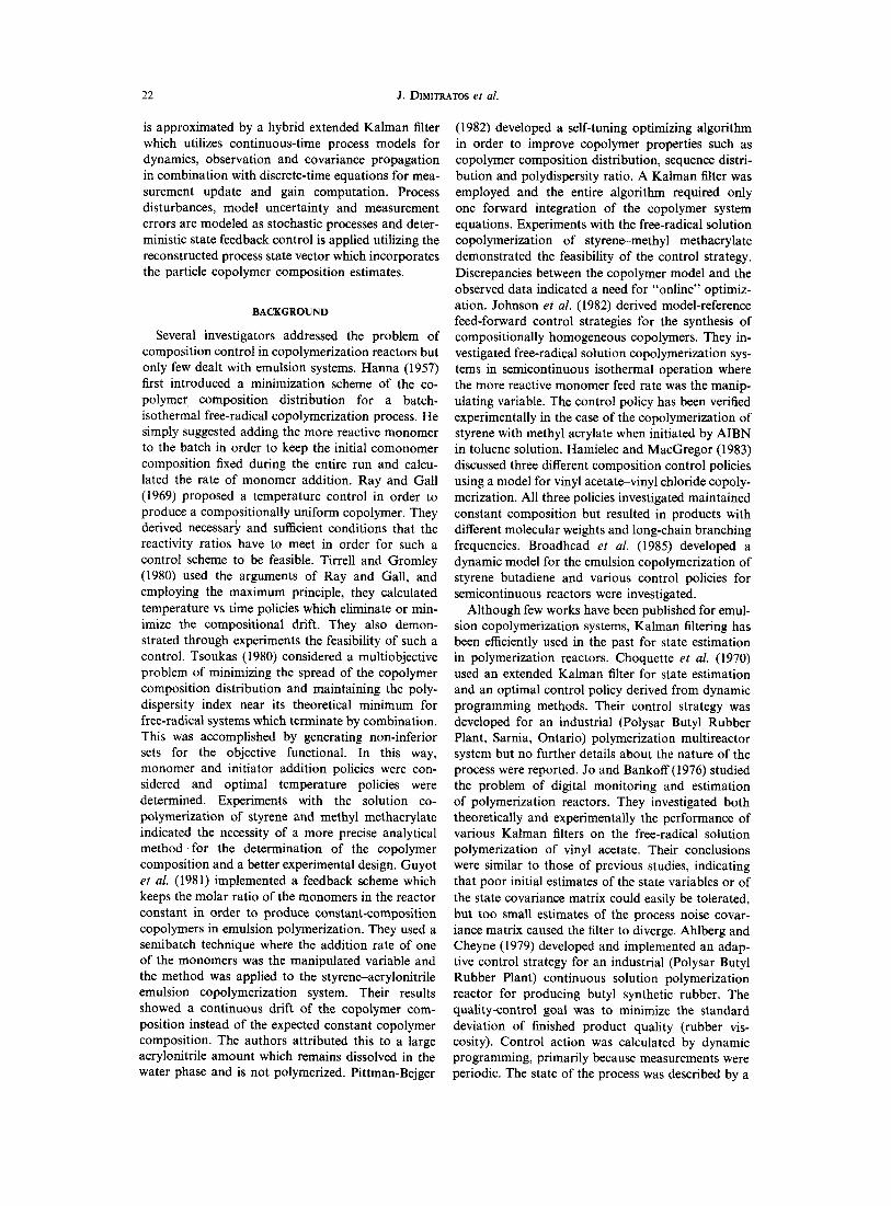
Fig. l. VAc distribution.

AG ( ~ ) 2 (IMP], [M~], ~1, ~2 )

\RT/2 ffM~], [M~], ~1, ~2}. (26)

These equations and their derivation are presented in Appendix A.

Since the only available measurements will be the overall residual monomers in the reactor, the observation model is defined by equation (19).

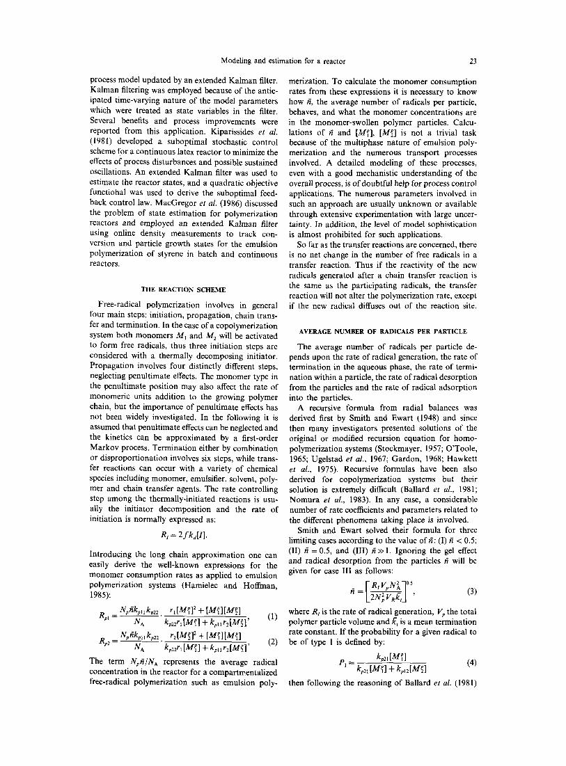
Simulations based on this complete model are shown in Figs l and 2. The distribution of the monomers between the different phases changes throughout the course of the polymerization and after the end of the monomer addition period, a drop in the level of monomers in the polymer particles is observed followed by a drop in the aqueous-phase monomer concentrations. This basically demon- strates the diffusion of the monomer from the aqueous phase into the polymer particles as modeled through the thermodynamic equilibrium approach.

t.0 - - I

._1 0 Z 0 . 8

I

Z

~ 0 . 6

~ 0 . 4 0

m 0 . 2

t . 2

O.

O. 2 .0 4 .0 6 . 0

TIME (HRS)

Fig. 2. BuA distribution.

The predicted aqueous phase monomer concentrations do not exceed the monomers' water solubility at the reaction temperature. As anticipated, BuA is quickly absorbed into the polymer particles and subsequently polymerized much faster than VAc which is accumulated up to a maximum concentration.

O N L I N E S T A T E E S T I M A T I O N

The model developed in the previous section accounts for the monomer distribution between the two phases by employing partition coefficients. These coefficients along with the average number of radicals per particle are calculated from certain expressions presented previously. A first attempt to state estimation is presented in the following by using a Kalman filter based on this model but without including any knowledge about the above-mentioned time- dependent parameters. The process model equations (21), (22), (24) and the observation model equation (19), can now be put into the more convenient vector form:

.¢c = g {x (t), p ( t ) , u(t)}, (27)

y = h { x ( t ) , p ( t ) } , (28)

where x is the state vector, g and h are vector-valued functions, p is a vector of time-varying parameters, u is the deterministic input vector and y is the observation vector. The measurements do not yield the entire state vector directly and are subject to errors. In addition, the process itself is subject to erratic disturbances which the model in its present form does not account for. One way to model these disturbances and errors is to describe them as stochastic processes and thus transform equations (27) and (28) into:

Yc = g { x (t), p ( t ), u( t ), w( t ) ) , (29)

y = h { x ( t ) , p ( t ) , n(t)), (30)

where w and n are random processes describing the process and measurement noise. Given the statistical description of w and n the problem is clearly to reconstruct the full state vector by estimating in the "optimum" sense the state variables. The "best" estimates in the stochastic environment are obtained by properly utilizing the information on the process dynamics and the available measurements. The solution to the linear case problem is given by the continuous-time Kalman-Bucy filter or the equivalent discrete-time Kalman filter (Kalman, 1960; Kalman and Bucy, 1961). Essentially these optimum filters are adaptive, gain-tuning techniques in which the prediction of the state vector at any time is weighted between the extrapolated past value of the state and the observed present value of the measurements. The model used by the filtering algorithm performs two functions: it directly propagates the time-varying mean value of the state vector estimate, and it enters into the calculation of the gains of the recursive minimum variance estimator.


Fairly straightforward extensions of the Kalman filter address the issue of nonlinearities or non- Gaussian effects. Modified linear-optimal estimators for nonlinear systems are very useful when the stochastic effects are additive (thus permitting sepa- ration of the deterministic part from the purely stochastic one) and small. Though not precisely "optimum" they are "suboptimal" in the sense that they tend to the optimum. Such a filter is the extended Kalman filter (Cox, 1964; Detchmendy and Sridhar, 1965; Noton and Choquette, 1968) which can be derived by local linearization about the best filter estimates and which permits online processing of each extra measurement as it becomes available. In the case of sampled-data measurements of a continuous process, a hybrid extended Kalman filter is most appropriate for state estimation (Stengel, 1986). The hybrid filter uses continuous-time models of dynamics, observation and covariance propagation in combination with the discrete-time equations for measurement update and gain computation.

The local linearization for the process model developed is presented in detail in Appendix B. The hybrid Kalman filtering equations have the following form:

state estimate propagation:

a? [ tk(-) ] = £[ tk_ l (+) ]

+ g{ i [ t ( - ) ] , u ( t ) }d t ; (31) , ) t ~ _ i

covariance estimate propagation:

P[ tk(- ) ] = P[t~_I(+)] + [G(t)P(t) d t~ 1

+ gz(t)Gr(t) + O_(t)Q(t)D_r(t)]dt; (32)

filter gain computation:

~(tk) = P[tk(--)]Hr(tk){H(tk)P[tk(--)]Hr(tk)

+ R(tk)}-~; (33)

state estimate update:

.r [tk(+)] = £ [tk(--)]

+ K(tk){y(tk)-- h(£ [tk(--)])}; (34)

covariance estimate update:

P[tk(+)] = [B -- K(tk)H(t~)]P[tk(--)]; (35)

where:

ag[.] Q_(t) ag[.] H(t) ah[.] G( t )= ~ = ~-w = c3x '

e{x(O)} = ~o E{[x(O) -,~o][x(O) - ~o f} = ~o,

E{(Wnl:l)(wr(t) n r ( t ) ) } = diag[Q, • ]6( t - s ) ,

E{wr(t)nr(t)} = O.

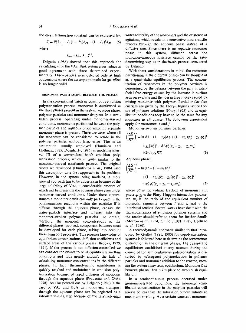
In the above equations ( - ) indicates that the update has not occurred, while ( + ) indicates updated values based on the most recent available measurements. E(tk) is the Kalman gain matrix and P(tk) is the state covariance matrix. The process and measurement noise vectors are assumed Gaussian "white" noise processes with mean zero. Note that the hybrid filter characterizes the stochastic disturbance input by its spectral density matrix and the measurement error by its covariance. The computational scheme for the state covariance propagation and update, and the filter gain calculation is presented in Fig. 3.

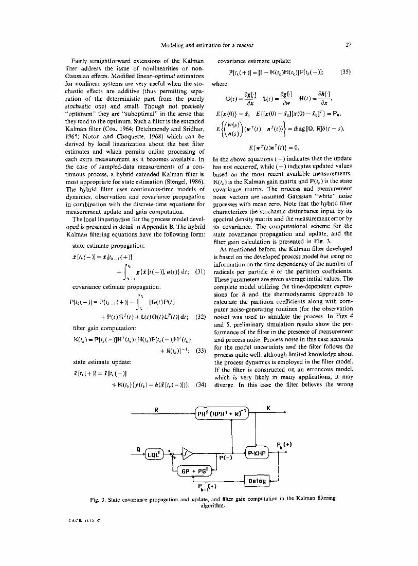
As mentioned before, the Kalman filter developed is based on the developed process model but using no information on the time dependency of the number of radicals per particle ri or the partition coefficients. These parameters are given average initial values. The complete model utilizing the time-dependent expressions for ri and the thermodynamic approach to calculate the partition coefficients along with computer noise-generating routines (for the observation noise) was used to simulate the process. In Figs 4 and 5, preliminary simulation results show the performance of the filter in the presence of measurement and process noise. Process noise in this case accounts for the model uncertainty and the filter follows the process quite well, although limited knowledge about the process dynamics is employed in the filter model. If the filter is constructed on an erroneous model, which is very likely in many applications, it may diverge. In this case the filter believes the wrong

Fig. 3. State covaria=nce propagation and update, and filter gain computation in the Kalman filtering algorithm.

C A.C E. 13 /1-2-~


o z

I

z n-

I11 x

u z o

2 . 4

t , 6

0 . 8

O0

O.

' | ' I I 1 .

2 . 0 4 . 0 6 . 0

TIME (HRS)

Fig. 4. Simulated reactor concentrations, as measured every 4 min.

extrapolation of the state too much and its "best" estimate could be wrong. This is most likely to take place when the state covariance matrix is too small or optimistic. To moderate this problem, the level of process noise must be carefully selected, so that it compensates for modeling errors. This corresponds to proper sizing of the process covariance Q which affects the magnitude of the state covariance matrix P. The magnitude of R relative to Q is an indication of the uncertainty of the observations and, hence, the degree of filter dependence on the observations. In our filter implementation the noise statistics were estimated online using information from the observation residuals. Thus, the noise true mean and its covariance were not assumed constant. That resulted in good filter tracking capabilities in presence of nonstationary process noise which was by no means white and Gaussian.

T H E N O I S E A D A P T A T I O N A L G O R I T H M

Although the basic assumptions behind the Kat- man filtering formulation are realistic, the problem of determining the statistics of even a white Gaussian noise process or measurement noise for a specific application still exists. In fact, this is a well-known

i--. B . 0

I 6 . 0

,,=,

4 . 0

2 , O I i ' ~ ' 0 .

O . 2 . 0 4 .0 6 . 0

TIME (HRS)

Fig. 5. Concentrations in polymer phase (solid lines represent true states, + represents estimates).

limitation in the application of Kalman filtering to real-world problems (Kalman and Bucy, 1961). Typically, the a pr ior i statistics are selected through analysis of empirical data or computer simulation and are assumed constant (Jazwinski, 1970). This usually involves a trial-and-error heuristic procedure which leads most of the time to acceptable filter performance. The process noise covariance matrix is usually taken to be diagonal both for convenience and for lack of information regarding covariances. Its diagonal elements are chosen to reflect the total possible error over the integrating interval (Mac- Gregor et al., 1986). The measurement of noise covariance matrix is relatively easier to obtain from knowledge of the measurement sensors, or from replicated measurement data. However, this approach may yield a satisfactory performance over some global operating regime but it will be inferior to that obtained when a priori statistics are locally known as a function of time. In addition to that, this heuristic approach still requires some good guesses of the noise statistics which might be difficult to obtain. Although more accurate modeling is an obvious solution, it is often an impractical and sometimes an impossible solution. An alternative approach adop- ted here is to "cover" modeling errors with noise and adaptively estimate the process and measurement noise covariances.

In real-world applications of the Kalman filter, the only quantities available to the engineer in judging filter performance are the residuals and their predicted statistics. The innovations process or the difference between the actual measurement vector and the predicted measurement vector (based on the observation model and the current state vector estimate) is such a residual. If the residuals are sufficiently small and consistent with their predicted statistics, then the filter performance is acceptable. A common pitfall is to judge the scheme's efficiency solely on the basis of the size of the residuals, and not on their statistical consistency. Rather than analyzing residuals after the fact, to determine filter performance, one could provide the filter itself with an adaptation mechanism for this purpose, as it is explained in the following. Such a computational scheme will provide feedback from residuals, in real- time, in terms of noise input levels. These will degrade the estimation error covariance matrix (i.e. increase the uncertainty), increase the filter gains, and thus "open" the filter to incoming data. Without such an adaptation mechanism and inexact a pr ior i statistics, the filter might diverge. This clearly occurs because the covariance matrix becomes unrealistically small (optimistic), the filter gain drops and subsequent measurements are ignored. The source of this filter behavior is definitely due to the fact that there is no way for the filter to check its own performance.

The problem of the parallel state and noise statistics estimation has been brought to the attention of many investigators and several schemes have been

Modeling and estimation for a reactor

proposed in the past with remarkable success, even in the presence of severe modeling errors (Jazwinski, 1968; Berkovec, 1969; Mehra, 1969; Sage and Husa, 1969; Hilborn and Lainiotis, 1969; Weiss, 1970; Tapley and Born, 1971; Mehra, 1972; Lainiotis, 1974; Alspach, 1974; Myers and Tapley, 1976). All the proposed "noise-adaptive" filters are based on ex- tracting the noise statistics information from the available residuals. The innovations process is used for the measurement noise statistics while a similar "artificial" residual is constructed for the plant noise. The reason for calling this second residual "artificial" will become apparent in the following, but the basic idea is that it is not based on an actual measurement but on an internal filter residual between the state propagation and its update.

For the observation noise statistics we consider the residual:

rj = yj - h (.~j), (36)

as an observation noise sample. If the noise samples rj are assumed to be representative of the true noise nj, they may be considered independent and identically distributed, and a simple parameter estimation problem can be constructed. An unbiased estimator of the mean of rj is given by the sample mean as follows:

1 u e = - - ~ rj. (37)

Nj= 1

An unbiased estimator for R is obtained by first constructing an estimator of the covariance of the residual as follows:

1 ~v /~ N - - l j = (rJ--f)(rJ--¢)r" (38)

It can be shown that an unbiased estimate of R is thus given by:

1 u ~ { ( r j - e ) ( r j - e ) r

~ = ' N - 1/=

N - 1 N H/DJ( - )Hr} ' (39)

For the state statistics, we use as a state noise sample the above mentioned "artificial" residual:

q j = i j ( + ) - - { ~ _ 1 ( + ) + _ g { i ( - ) , u } d t } . (40)

If the qj are assumed to be representative of w then they can be considered independent and identically distributed and an unbiased estimator of the mean of the residual can be constructed in the same way as for the measurement noise mean:

1 ~ = ~1 qj" (41)

The covariance of the residual is estimated in the same way as:

1 _ ~ (qj _ # ) ( q j _ # ) r . ( 4 2 )

Q N - l / = =1

29

The estimator for the state noise covariance is thus given by:

] u (

l ~ = N - - ij ~.=1 (qJ--gl)(qs--gl)r NN 1

XI~j--I(-~)-~jJ I[GP-~-"~T]dt--Pj('q-)]} • (43)

THE LIMITED MEMORY FILTER

The major assumption in the derivations of the previous section was the constant characteristics of the noise statistics. Since it is most probable that these statistics are time-varying, the already presented "batch" type noise estimators were modified, so that they would be able to efficiently track nonstationary noise processes. This could be the case of batch-to- batch variations in charge, variations in impurity levels or model parameters. A limited memory filter approach was considered in which only a certain number of past noise samples was utilized by the estimators to obtain the local noise statislics. A "moving window" of samples was thus stored and the batch algorithms were transformed into sequential estimators using a shifting operation which discards the "oldest" samples as soon as new are available. The efficiency of this algorithm was tested in simulations by introducing random noise in the observations and modeling inaccuracies in the filter. Biases were initialized with zero values, but quickly converged to the true noise mean.

CONCLUSIONS

The process under investigation represents a difficult control problem. The composition of the copolymer product cannot be measured online, the available measurements are limited and a detailed modeling requires numerous parameters available only through extensive experimentation and with questionable confidence. The theoretical development of a model for this process has been summarized in this work. The model accounts for the distribution of the monomers in the different phases of the system employing a thermodynamic approach and predicts the time-dependent average number of radicals per particle. Thus, the compartmentalized nature of the system has been incorporated in our model to that extent which permits satisfactory pre- dictions with reasonable computational effort for a process control application. An extended hybrid Kalman filter has been designed, based on the local linearization of the model, around the suboptimal filter estimates, and preliminary estimation studies were conducted. With proper adaptation of the noise covariance, the filter can efficiently cope with cor- rupted measurements and model uncertainty, recon- structing the full state vector which is not directly available from the online observations. The filter


e s t i m a t e s a re n e c e s s a r y to i m p l e m e n t a p r o d u c t qua l -

i ty c o n t r o l s t r a t egy w h i c h will l ead to " t a i l o r m a d e "

c o p o l y m e r s o f des i red c o p o l y m e r c o m p o s i t i o n .

N O M E N C L A T U R E

d i= Monomer density (kg m 3) dp = Polymer density (kg m -3) Fi = Monomer feed rate (kmol s - l ) f = Initiator efficiency factor

(AC/RT) q = Dimensionless partial molar free energy of monomer i in phase q

[I] = Initiator concentration in aqueous phase (kmol m -3)

kd= Initiator decomposition rate constant (s -1) kp~, = Propagation rate constant (m 3 kmo l - l s - ~ ) kp,: = Cross propagat ion rate constant

(m 3 kmol - i s - i ) k ,~=Termina t ion rate constant (m3kmol -~s - l ) k w = Cross termination rate constant

(m 3 kmol i s - 1 ) /~t = Mean overall termination rate constant

(m 3 kmol - 1 s l ) [Mq] = Unreacted monomer i concentration in phase

q(kmol m 3 o f phase q) [M:] = Unreacted monomer i concentration in reac-

tor (kmol m -3 o f latex) 3~W, = Monomer molecular weight

m q = R a t i o of equivalent number of molar segments between i and j

m~p= Ratio of equivalent number of molar segments between i and polymer

m~w=Ratio of equivalent number of molar segments between i and water

N = Total number of particles Np = Number of particles per unit volume of latex

(m -3) NA = Avogadro 's constant

ri = Average number of radicals per particle P~ = Probability for a radical to be of type i R, = polymerization reaction rate (kmol s - t ) Rpj=Polymerizat ion reaction rate ( kmo l s - t 1 -1 ) Rz = Initiator decomposition rate (kmol s - t 1 - t ) R = Universal gas constant (J m o l - 1 K - t ) r, = Reactivity ratio rp = Radius of the polymer particles (m3) T = Reaction temperature (K)

Vq = Total volume of phase q(m 3) VR = Total reactor volume (m 3) V~ = Water volume in aqueous phase (m 3)

Greek symbols =t, = Partition coefficient

= Copolymer interfacial tension (N m - 1 ) p, = Molar monomer density (mol m 3)

~b q = Volume fraction of monomer i in phase q ~b~ = Volume fraction o f polymer in polymer phase ~b a = Volume fraction of water in aqueous phase z u = M o n o m e r - m o n o m e r Flory-Huggins inter-

action parameter Z,p = Monomer -po lymer Flory-Huggins inter-

action parameter X,~ = Monomer-wate r Flory-Huggins interaction

parameter

Subscripts i = 1, for VAc i = 2, for BuA

q = a, for aqueous phase q = p, for polymer particles

Superscripts q = a, for aqueous phase q = p, for polymer particles

Vector notation G(t) = Process model Jacobian matrix g(t) = Process model vector valued function H(t) = Observation model Jacobian matrix h(t) = Observation model vector valued function

= Identity matrix ~( t ) = Ka lman gain matrix n(t) = Measurement noise vector p(t) = Parameter vector P(t) = State covariance matrix estimate

P0 = Initial state covariance matrix estimate ~(t) = Process noise mean estimate q(t) = Process noise sample vector Q(t) = Process noise covariance matrix O(t) = Process noise covariance matrix estimate f ( t ) = Observation noise mean estimate r(t) = Observation noise sample vector ~(t) = Measurement noise covariance matrix ~(t) = Measurement noise covariance matrix esti-

mate u(t) = Deterministic input vector w(t) = Process noise vector x(t) = State vector .f(t) = State vector estimate

J~0 = Initial state vector estimate y(t) = Observation vector

R E F E R E N C E S

Ahlberg D. T. and I. Cheyne. Adaptive control o f a polymerization reactor. A1ChE Syrup. Ser. Chem. Process Control 159, 221-229 (1979).

Alspach D. L. A parallel filtering algorithm for linear systems with unknown time-varying statistics. IEEE Trans. Automat. Control AC-19, 55~556 (1974).

Ballard M. J., D. H. Napper and R. G. Gilbert. Theory of emulsion copolymerization kinetics. J. Polymer. Sci: Polymer Chem. Edn 19, 939-954. (1981).

Berkovec J. W. A method for the validation of Ka lman filter models. Preprints o f the lOth Joint Automatic Control Conf. Am. Automatic Control Council, University of Col- orado, Boulder. pp. 488493 (1969).

Broadhead T. O., A. E. Hamielec and J. F. MacGregor. Dynamic modeling of the emulsion copolymerization of styrene/butadiene. Makromol. Chem. Suppl. 10/11, 105-128 (1985).

Brooks B. W. Mass transfer and thermodynamic effects in emulsion polymerization. British Polymer J. 2, 197-201 (1970).

Brooks B. W. Interfacial and diffusion phenomena in emulsion polymerization. British Polymer J. 3, 269-273 (1971).

Choquette P., A. R. M. Noton and C. A. G. Watson. Remote computer control o f an industrial process. Proc. IEEE 58, 10-16 (1970).

Cox H. On the estimation o f state variables and parameters for noisy dynamic systems. 1EEE Trans Automatic Con- trol AC-9, 5-12 (1964).

Delgado J. Miniemulsion copolymerization of vinyl acetate and N-butyl acrylate. Doctoral dissertation, Lehigh Uni- versity, Bethlehem, Penn. (1986).

Detchmendy D. M. and R. Sridhar. Sequential est imation of states and parameters in noisy nonlinear dynamical systems. Proc. Joint Automatic Control Conf., Troy, New York (1965).

Dimitratos J., C. Georgakis, M. E1-Aasser and A. Klein. Research progress report No. 2. Chemical Process Mod- eling and Control Center, Lehigh University (1986).

Dougherty E. P. The SCOPE dynamic model for emulsion


polymerization I. Theory. J. Appl. Polymer Sci. 32, 3051-3078 (1986).

Flory P. J. Principles of Polymer Chemistry. Cornell Univer- sity Press, New York (1953).

Gardon J. L. Emulsion polymerization. V. Lowest theoretical limits of the ratio kt/k p. J. Polymer Sci: Part A- 1 6, 2853-2857 (1968).

Guillot J, Kinetics and thermodynamic aspects of emulsion copolymerization. Acrylonitrile-styrene copolymerization. Acta Polymer 32, 593~500 (1981).

Guillot J. Some thermodynamic aspects in emulsion copolymerization. Makromol. Chem. Suppl. 10]11, 235-264 (1985).

Guyot A., J. Guillot, C. Pichot and L. R. Guerrero. New design for producing constant-composition copolymers in emulsion polymerization. In Emulsion Polymers and Emulsion Polymerization (D. R. Basset and A. E. Ham- ielec, Eds). ACS Symp. Ser. Washington, D.C. (1981).

Hamielec A. E. and T. W. Hoffman. Emulsion Poly- merization. Course Notes, McMaster Institute for Polymer Production Technology (1985).

Hamielec A. E. and J. F. MacGregor. Modeling copolymerizations--control of chain microstructure, molecular weight distribution, long chain branching and crosslinking. Proc. Int. BeHin Wkshp Polymer Reaction Engng, Berlin (1983).

Hanna R. J. Synthesis of chemically uniform copolymers. Ind. Engng Chem. 49, 208-209 (1957).

Hawkett B. S., D.:H. Napper and R. G. Gilbert. Emulsion polymerization kinetics, J. Chem. Soc: Faraday Trans I 71, 2288-2295 (1975).

Hilborn C. G. and D. G. Lainiotis. Optimal estimation in the presence of unknown parameters. IEEE Trans Syst Sci., Cybernet. SSC-5, 38-42 (1969).

Jazwinski A. H. Adaptive filtering. IFAC Symp. Multi- variable Control Syst. Dusseldorf, 7-8 October (1968).

Jazwinski A. H. Stochastic Processes and Filtering Theory. Academic Press, New York (•970).

Jo J. H. Digital monitoring and estimation of polymerization reactors. Doctoral Dissertation, Northwestern University, Evanston (1975).

Jo J. H. and S. G. Bankoff. Digital monitoring and estimation of polymerization reactors. AIChE J122, 361-369 (1976).

Johnson A. F., B. Khaligh and J. Ramsay. Controlled and uncontrolled semi-batch solution copolymerization of styrene with methyl acrylate. In Computer Applications in Applied Polymer Science (T. Provder, Ed). ACS Syrup. Ser. Washington, D.C. (1982).

Kalman R. E. A new approach to linear filtering and prediction problems. Trans ASME, J. Basic Engng 82, 35-45 (1960).

Kalman R. E. and R. S. Bucy. New results in linear filtering and prediction theory. Trans ASME, J, Basic Engng 83D, 95-108 (1961).

Kiparissides C., J. F. MacGregor and A. E. Hamielec. Suboptimal stochastic control of a continuous latex reactor. AIChE Jl 27, 13-20 (1981).

Lainiotis D. G. Partitioned estimation algorithms I: nonlinear estimation. Inform. Sei. 7, 203-235 (1974).

MacGregor J. F., D. J. Kojub, A. Penlidis and A. E. Hamielec. State estimation for polymerization reactors. IFAC Symp. Dynamics Control Chem. Reactors Dis- tillation Columns, Bournemouth, U.K. (1986).

Mehra R. K. On the identification of variances and adaptive Kalman filtering. Preprints of the lOth Joint Automatic Control Conf. Am. Automatic Control Council, University of Colorado, Boulder. pp. 495-505 (1969).

Mehra R. K. Approaches to adaptive filtering. IEEE Trans Automat. Control AC-17, 693~98 (1972).

Morton M., S. Kaizerman and M. W. Altier. Swelling of latex particles. J. Colloid Sci. 9, 300-312 (1954).

Myers K. A. and B. D. Tapley. Adaptive sequential esti-

mation with unknown noise statistics. IEEE Trans Auto- mat. Control AC-21, 520-523 (1976).

Nomura M., M. Kubo and K. Fujita. Kinetics of emulsion polymerization--Ill. Prediction of the average number of radicals per particle in an emulsion copolymerization system. J. Appl. Polymer Sci. 28, 2767-2776 (1983).

Noton A. R. M. and P. Choquette. Application of modern control theory to the operation of an industrial process. Proc. IFAC/IFIP Symp., Toronto, Canada (1968).

O'Toole J. T. Kinetics of emulsion polymerization. J. Appl. Polymer Sci. 9, 1291-1297 (1965).

Pittman-Bejger T. P. Real-time Control and Optimization of Batch Free-radical Copolymerization Reactors. Doctoral dissertation, University of Minnesota (1982).

Prausnitz J. M. and T. Oishi. Estimation of solvent activities in polymer solutions using a group-contribution method. Ind. Engng Chem: Process Des. Dev. 17, 333-339 (1978).

Ray W. H. and C. E. Gall. The control of copolymer composition distributions in batch and tubular reactors. Macromolecules 2, 425-428 (1969).

Sage A. P. and G. W. Husa. Adaptive filtering with unknown prior statistics. Preprints of the lOth Joint Auto- matic Control Conf. Am. Automatic Control Council, University of Colorado, Boulder. pp. 760-769 (1969).

Smith W. V. and R. H. Ewart. Kinetics of emulsion polymerization. J. Chem. Phys. 16, 592-599 (1948).

Stengel R. F. Stochastic Optimal Control. Wiley, New York (1986).

Stockmayer W. H. Note on the kinetics of emulsion polymerization. J. Polymer Sci. 24, 314-317 (1957).

Tapley B. D. and G. H. Born. Sequential estimation of the state and the observation-error covariance matrix. AIAA 'Jl 9, 212-217 (1971).

Tirrell M. and K. Gromley. Composition control of batch copolymerization reactors. Chem. Engng Sci. 36, 367-375 (1980).

Tsoukas A. A. Multiobjective Analysis and Control of Semi-batch Copolymerization Reactors. Master's Thesis, University of Minnesota (1980).

Ugelstad J., P. C. Mork and J. O. Aasen. Kinetics of emulsion polymerization. J. Polymer Sci: Part A-I 5, 2281-2288 (1967).

Ugelstad J., P. C. Mork, K. H. Kaggerud, T. Ellingsen and A. Berge. Swelling of oligomer-polymer particles. New methods of preparation of emulsion and polymer dis- persions. Adv. Colloid Interface Sci. 13, 101-140 (1980).

Weiss I. M. A survey of discrete Kalman-Bucy filtering with unknown noise covariances. Presented at the AIAA Guid- ance, Control and Flight Mechan. Conf., Aug. 17-19 (1970).

APPENDIX A

Derivation of the Mathematical Model Equations From equations (19) and (20) we obtain:

[Mr] =f , [Mq],

IMp] =AIM% where:

f'([Mq]'[M~]':t"°t2" VR)= ~PR( l - l-~+ o:,

f2([M~], [M~], ~,, ~2, VR) = ~ 1 -- + --'e2

and from equation (24):

dVR =g4 dt

32 J. DIMITRATO$ et al.

where:

g,([M~l, [M~], Vl, F2, [I])

FIMW~ [_F2MW 2 a~ a~

1 1\ / 1 1~ - - - -- - - / - R~ M W 2 l - - -- - - / . R ' M W ' d , dr, ] \d2 dv/I

Substituting back into equations (8) and (9), we obtain:

d(A [M~1) F~ - R, - - V~ + g4A[Mq],

dt

d(f2[M~]) F z -- R2 d ~ V~ + g4f2[M~].

Carrying out the differentiations and rearranging we obtain:

v .

= El -- RI -- g 4 f l [M~] - - [ M q ] V . ~ g4,

{ f ~ V l ~ + M V Of~ )d[M~I ~[M~]VR Ofz ~d[M~] [ ~]

0A = F 2 - R 2 - g, f2 [M~] -- [M~]V~-~g~.

This system of equations can be solved for the derivatives of the monomer concentrations, the solution being:

d[M~] A2KI -- B, K 2 gt ([M~], [M~],

dt A ~ A 2 - B~B~

Vs, a~, a2, FI, F2, [I]),

d[M~] AIK: -- B:K, g~ ([Mq], [M~],

dt A I A 2 - B I B 2

V~, al, a2, FI, F 2, [I]),

where:

of, ~, = f, v . + [M'dVR o~-¢f

OA Az =fz V~ + [M~]V~ ~[~z] ,

0f, B 1 = [Mq]V n 0[Mp] '

oA ,~ = IMPLY. 0~-~1'

0f~ KI = F, -- R l -- g4fl [gl ] -- [Mq] V~ ~ g4,

0f~ K2 = F~ - R~ -g4f2 [M~] - [MP] V~ ~7-g4, ~vR

with:

of, (1 -A)~ v~ 0[MP] p l ( ~ l - I)V~'

Of~ (1 -A) (1 --A)V~

O[M~] p l ( ~ l - - 1)V~ '

0 A (1 -f~)(1 -A)VR

O[M~I P2(~z- 1)V~ '

0A (1 - A ) 2 v~ 0[M~] p2(a 2 -- 1)V~'

Of~ 1 - A OA 1 - f z or. v . ' or . v .

A P P E N D I X B

Local Linearization The original nonlinear model is linearized locally around a nominal trajectory defined by [M~]o, IMP]o, VRo, FIo,F2o. The linearized equations are:

d[~'~"~] Og I og, I .e., dt O[M~] o O[M{] o OVR o

d[~'~l Og2 Og2 Og2

atM,] o O[M~] o o r . o dt t ~ v . [ 3 . 7 { ] + - - " [ 3 ~ ] + - - • i7..

d V R Og 4 Og 4 Og 4 I dt O[Mf] o'['A~f] + ~ o ' [ M ~ ] + ~ o "[7"'

The Jacobian elements are given by:

Ogl (AIA2 - B, B2)(A~K, + A2K; - B~K2 -- BtK;)

-- (A2KI - BIK2)(A ~ A2 + AIA" 2 - B~B 2 - B1B~)

Oxi (AIA2 -- BIB2) 2 '

(AIA 2 -- BIB2)(A ~K2 + AIK" z - B'zK 1 - B2K ~ ) Og 2 -- (A,K2--B2KI)(A'IA2+ A I A ~ - B ' I B 2 - B , B ~ )

OX i (A I A2 -- B102 )2 '

_ , , . . ( ) Og 4 f ~ R ~ M W I _ 1 1 Ox, \all d,/ R' MW ,

where x i stands for any of [Mr], [M2 p] or V R, and the primes denote partial derivatives of the functions defined in Appendix A with respect to x i. These partial derivatives are calculated as follows:

With respect to [M~]:

OA~ =2 OA V R. 14 0[Mfl 0[Mfl p ~ - 1 ~ J '

OA2 0A f 2[M2P](1 - f2 ) VR) 0[Mf] =0tM,q. VR..I+ I'

OB, 0A { 2[Mfl(1 - A ) V.~ O[M~]=O[M~] "VR" l + ~ - - l ~ w -j,

0B 2 0 A 2[M~] ( I - A ) V .

0[Mr] =O[Mf~] "V" p , ( ~ , - 1)V~

0KI R~ -- g4 -- [MP]g'4,

[Mr]

[Mr] R~ -- [M~]g'4,

0R, ,~Nkp,,k~22 m

0 [M p ] NA

(2r I [Mr] + [M~]) (kp2 2 r,[M~] + kp, I r 2 [M~ 1) - (rl[Mf] 2 + [Mfl[M~l)rlkp22

OR2 o [Mf]

(kp2 2 r I [M f ] + kp,, r 2 [M ~ 1) 2

~Nkvukv22

U~

[g~](kv22rt[g f] + kvur2[g~]) × - - ( r 2 [ M f ] 2 + [Mf][M~])rlkv22


With respect to [M~]:

~A 1 6~fl

~[M~] ~[M~] V R • {1 + 2[Mf](l - f l ) VR~

~3A2 . : OA .{1 [M~I(1--A)VR~ t Ti z"

OBx c3f~ 2[Mf](1 --f2)V R c~[M~] ' c3[M~] VR p2(~2- 1)V$ '

_ { 2[M~I(1 - f2) V,~ OB2 ~f2 . VR. 1+ O[M~] O[Mf] p2(u2- 1)V~, ) '

[M~](k,22rl[M~] + krll r2[M~]) ] -- (r I [M~] 2 + IMf][M~J)r2kpll

(kp2 2 r I [M~] + kpl I r 2 [M~])2

~& ~Nk~,l kp22 ~[M~] N~

"(2rz [M~] + [Mq]) (kp22 r I [M~] ] + kpll r2[M~]) -- (r2 [M~] 2 + [M~l[M~l)r2kptl

(kp2 2 r I [M~] + kpu r: [M p 1) 2

R~ -- [M{]g~, d[M~]

~K2 R~ -- g, -- [M2Plg~, O[M{]

OR l tiNkt, u kp2z

~[M~] N~

With respect to VR: OA 1 ~3A z aB l OB 2 O-~R=I, ~ = 1 , ~V~R=0, ~ = 0 ,

OKl c~K2 ORt 0 3R~ - - = 0 , =0,

dynamic modeling and state estimation for an emulsion copolymerization reactor

Documents