dynamic factor models and realized volatility: an application to

Dynamic factor models and realized volatility: Anapplication to forecasting bond yield distributions

Minchul Shin and Molin Zhong

University of Pennsylvania

July 16, 2013

Copyright c©2013 by Minchul Shin and Molin Zhong. All rights reserved.

Minchul Shin and Molin Zhong (UPenn) DNS July 16, 2013 1 / 24

Introduction

1 We study a method to incorporate realized measures of volatilityinto the dynamic factor model.

Dynamic factor model with time-varying volatilityBetter density prediction with realized volatility

2 We apply this method to US Bond-Yield density forecasting.Dynamic Nelson Siegel Model, Diebold and Li (2006)Density forecast evaluation for the DNS model


Outline

1 Model/Methoda) DNS Modelsb) Incorporating realized measures of volatility

- Univariate stochastic volatility model- Extension to the dynamic factor model framework

2 Application to forecasting government bond yield distributiona) Estimation resultb) Forecasting result


Dynamic Nelson Siegel Model (DNS-C)Diebold and Li (2006)

yt = Λ f (λ)

ltstct

+ εt (1)

lt −µlst −µsct −µc

= Φ

lt−1 −µlst−1 −µsct−1 −µc

+ηt (2)

�

εtηt

�

∼ N�

0,�

Q 00 Σ

��

(3)

Dynamic factor model with Λ f (λ)Smooth functional form approximation of yield curve. Can capture manydifferent shapes of the yield curve.Factors interpreted as lt (level), st (slope), and ct (curvature).

Good performance both in-sample and out-of-sample forecasting.


DNS Model with Stochastic Volatility (DNS-SV)

�

εtηt

�

∼ N�

0,�

Q 00 Σt

��

(4)

Σt =

exp(hl,t) 0 00 exp(hs,t) 00 0 exp(hc,t)

(5)

hi,t −µh,i = φh,i(hi,t−1 −µh,i) + ei,t (6)

ei,t ∼ N(0,σ2i ) (7)

Bianchi, Mumtaz, and Surico (2009), Hautsch and Ou (2012), Hautsch and Yang(2012)


DNS Model with Stochastic Volatility (DNS-SV)

�

εtηt

�

∼ N�

0,�

Q 00 Σt

��

(4)

Σt =

exp(hl,t) 0 00 exp(hs,t) 00 0 exp(hc,t)

(5)


ei,t ∼ N(0,σ2i ) (7)

Suppose we have volatility measures (proxies) for yt

We want to use them to get better estimates for volatility factor ht

Link volatility proxies to latent volatility factor ht


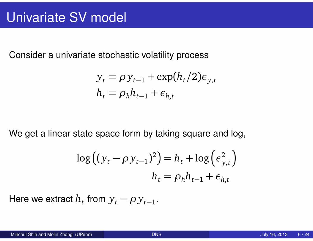
Univariate SV model

Consider a univariate stochastic volatility process

yt = ρ yt−1 + exp(ht/2)εy,t

ht = ρhht−1 + εh,t

We get a linear state space form by taking square and log,

log�

(yt −ρ yt−1)2�

= ht + log�

ε2y,t

�


Here we extract ht from yt −ρ yt−1.


Univariate SV model with high-frequency data

Suppose we have a proxy for ht , RMt .

Range-based volatility, realized volatility, ...

Measures based on high-frequency data. They can be moreinformative than differenced data.

Then one can extract ht based on

RMt = α+ βht + εRM ,t


Again, this is a linear state space form.

Alizadeh, Brandt and Diebold (2002), Barndorff-Nielsen andShephard (2002)


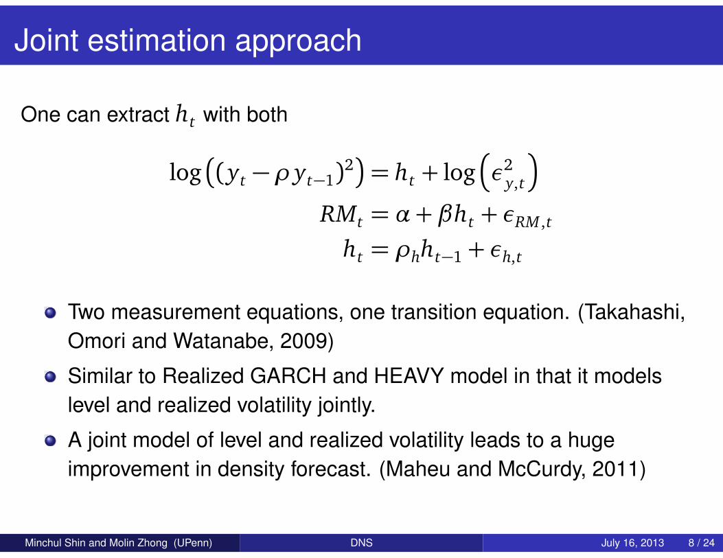
Joint estimation approach

One can extract ht with both

log�

(yt −ρ yt−1)2�

= ht + log�

ε2y,t

�

RMt = α+ βht + εRM ,t


Two measurement equations, one transition equation. (Takahashi,Omori and Watanabe, 2009)

Similar to Realized GARCH and HEAVY model in that it modelslevel and realized volatility jointly.

A joint model of level and realized volatility leads to a hugeimprovement in density forecast. (Maheu and McCurdy, 2011)


Extension to dynamic factor models

Now we want to extend this idea to the dynamic factor model setting,

yt = λ f ft + εy,t

ft = Φ f ft−1 + ε f ,t , ε f ,t ∼ N�

0,Σt

�

where Σt = diag�

exp�

h1,t

�

, ..., exp�

hJ ,t

��

,

h j,t = ρh, jh j,t−1 +σ jεh,t , j = 1, ..., J

and

N : dimension of yt , usually large

J : dimension of ft , usually small

Time-varying volatility of factors (ht ) drives time-varying volatility ofyt as well.


Extracting ht

Estimation of ht is similar to univariate SV case. Given ft and otherparameters,

log�

�

ft −Φ f ft−1

�2�

=

h1,t...

hJ ,t

+η f ,t

h j,t = ρh, jh j,t−1 +σ jεh,t j = 1, ..., J

Now suppose we have external information about volatility, RMt asbefore. We want to use them but it is hard because

Volatility proxy for factors is not available.

But volatility proxy for yi,t is available, RMi,t for i = 1, ..., N .


New volatility measurement equationNatural way of linking volatility factor (J × 1) to individual volatility proxies (N × 1) is toimpose factor structure,

log�

�

ft −Φ f ft−1

�2�

=

h1,t...

hJ ,t

+η f ,t

RMt= ch+λh

h1,t...

hJ ,t

+ x t

h j,t = ρh, jh j,t−1 +σ jεh,t

Two sets of measurement equations and one set of transition equations.

λh links J volatility factor to N individual volatility proxies. N × J matrix.

In the paper

Justification for the factor structure.λh is a function of other parameters. No additional parameter to beestimated.


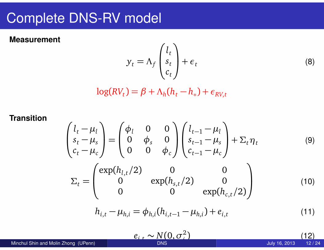
Complete DNS-RV modelMeasurement

yt = Λ f

ltstct

+ εt (8)

log(RVt) = β +Λh(ht − h∗) + εRV,t

Transition

lt −µlst −µsct −µc

=

φl 0 00 φs 00 0 φc

lt−1 −µlst−1 −µsct−1 −µc

+Σtηt (9)

Σt =

exp(hl,t/2) 0 00 exp(hs,t/2) 00 0 exp(hc,t/2)

(10)


ei,t ∼ N(0,σ2i ) (12)


Data and Models

Data (Christensen, Lopez and Rudebusch, 2010)

(yt) Monthly US zero coupon bonds yield data (Jan 1981 ∼ Dec2011).

(RVt) Daily US zero coupon bonds yield data to construct monthlyrealized volatilities

17 yields with maturities 3, 6, 9, 12, 15, 18, 21, 24, 30, 36, 48, 60,72, 84, 96, 108, 120 months.

Models

DNS-C: Constant volatility

DNS-SV: Stochastic volatility model

DNS-RV: Realized volatility model (Proposed method)


US Yield Data

Yield % variance explained

pc1 98.11pc2 99.86pc3 99.98pc4 100.00pc5 100.00


RV in logs

ln(RV) % variance explained

pc1 82.17pc2 93.73pc3 98.20pc4 99.39pc5 99.81


Estimation and Forecasting

EstimationBayesian estimation, Gibbs Sampler

Loose priors.50,000 draws.

ForecastingPoint and density forecast comparison.

Estimation sample starts: Jan 1981Forecasting origin starts: Oct 1998Estimate model and generate forecasts for every 2-months. (80repetitions)Forecast horizons 1 month ahead to 12 months ahead


Stochastic volatility: DNS-RV versus DNS-SV


Density forecasting evaluation

Probability Integral Transforms (PITs)

PI TT =

yT+h∫

−∞

p(yT+h|Y1:T )d yT+h (13)

where p(yT+h|Y1:T ) is the predictive density. If the predictive density iswell-calibrated, then

For all h, PI Tt should be marginally uniformly distributed.For h= 1, PI Tt should also be iid.

DNS-RV specificationgives better predictive distribution for most cases than othercompetitors.especially performs better for middle range maturities. (24m ∼60m)


Density forecast comparison: PITs

Left: DNS-C, Middle: DNS-SV, Right: DNS-RV

PITs: 1-Month-Ahead Prediction


Conclusion

We discuss how to incorporate realized measures of volatility into thedynamic factor model framework.

We show that DNS-RV produces more accurate predictive distribution. Inthe paper,

DNS-RV performs the best in terms of point prediction as well.(RMSE)

More on the density prediction evaluationPIT independenceLog predictive density

Future work: Incorporating “realized covariance”


dynamic factor models and realized volatility: an application to

Documents