bootstrap inference for pre-averaged realized volatility ...€¦ · bootstrap inference for...
TRANSCRIPT

Bootstrap inference for pre-averaged realized volatility based on
non-overlapping returns ∗
Sılvia Goncalves†, Ulrich Hounyo‡and Nour Meddahi§
Universite de Montreal, University of Oxford, and Toulouse School of Economics
December 2, 2013
Abstract
The main contribution of this paper is to propose bootstrap methods for realized volatility-likeestimators defined on pre-averaged returns. In particular, we focus on the pre-averaged realizedvolatility estimator proposed by Podolskij and Vetter (2009). This statistic can be written (up to abias correction term) as the (scaled) sum of squared pre-averaged returns, where the pre-averagingis done over all possible non-overlapping blocks of consecutive observations. Pre-averaging reducesthe influence of the noise and allows for realized volatility estimation on the pre-averaged returns.The non-overlapping nature of the pre-averaged returns implies that these are asymptotically un-correlated, but possibly heteroskedastic. This motivates the application of the wild bootstrap inthis context. We provide a proof of the first order asymptotic validity of this method for percentileand percentile-t intervals. Our Monte Carlo simulations show that the wild bootstrap can improvethe finite sample properties of the existing first order asymptotic theory provided we choose theexternal random variable appropriately. We use empirical work to illustrate its use in practice.
Keywords: High frequency data, realized volatility, pre-averaging, market microstructure noise,wild bootstrap.
1 Introduction
The increasing availability of financial return series measured over higher and higher frequencies (e.g.
every minute or every second) has revolutionized the field of financial econometrics over the last decade.
Researchers and practitioners alike now routinely rely on high frequency data to estimate volatility
(and functionals of it, such as regression and correlation coefficients).
∗We would like to thank Ilze Kalnina for many useful comments and discussions. We would also like to thank theeditor in charge, Allan Timmermann, as well as two anonymous referees for their comments and suggestions, whichgreatly improved the paper. This work was supported by grants FQRSC-ANR and SSHRC. In addition, Ulrich Hounyoacknowledges support from CREATES - Center for Research in Econometric Analysis of Time Series (DNRF78), fundedby the Danish National Research Foundation, as well as support from the Oxford-Man Institute of Quantitative Finance.Finally, Nour Meddahi benefited from the financial support of the chair “Marche des risques et creation de valeur”Fondation du risque/SCOR.†Departement de sciences economiques, CIREQ and CIRANO, Universite de Montreal. Address: C.P.6128, succ.
Centre-Ville, Montreal, QC, H3C 3J7, Canada. Tel: (514) 343 6556. Email: [email protected].‡Oxford-Man Institute of Quantitative Finance and CREATES, University of Oxford. Address: Eagle House, Walton
Well Road, Oxford OX2 6ED, UK. Email: [email protected].§Toulouse School of Economics, 21 allee de Brienne -Manufacture des Tabacs-31000, Toulouse, France. Email:
1

One earlier popular estimator was realized volatility, computed as the sum of squared intraday
returns. This is a consistent estimator of integrated volatility (a measure of the ex-post variation of
asset prices over a given day) under quite general assumptions on the volatility process. However, one
important assumption underlying the consistency of realized volatility is the assumption that markets
are frictionless (so that asset prices are observed without any error). This assumption does not hold
in practice. As the sampling frequency increases, market microstructure effects such as the existence
of bid-ask bounds, rounding errors, discrete trading prices, etc, contribute to a discrepancy between
the true efficient price process and the price observed by the econometrician (known as the market
microstructure noise).
The negative impact of market microstructure effects on realized volatility is now an accepted fact
in the econometrics literature of high frequency data. A number of alternative estimators have been
proposed that take into account these effects (see e.g. Zhou (1996), Zhang et al. (2005), Hansen and
Lunde (2006), Bandi and Russell (2008), Barndorff-Nielsen et al. (2008), Podolskij and Vetter (2009)
and Jacod et al. (2009)). Although these estimators rely on a large number of high frequency returns,
finite sample distortions associated with the first order normal approximation may persist even at
large sample sizes, as shown by our simulations.
In this paper, we consider the bootstrap as an alternative method of inference. We focus on
the pre-averaging approach of Podolskij and Vetter (2009), where we first “average” the observed
noisy returns over given blocks of non-overlapping observations, and then apply the standard realized
volatility estimator to the pre-averaged returns. By averaging returns, the impact of the market
microstructure noise is lessened, thus justifying realized volatility-like estimation on the pre-averaged
returns. The class of statistics that we consider can be written (up to a bias term) as the (scaled)
sum of squared pre-averaged returns (using an appropriate weighting function) computed over non-
overlapping intervals. Our proposal is to bootstrap the pre-averaged returns.
Jacod et al. (2009) propose a generalization of the pre-averaging approach of Podolskij and Vetter
(2009) which entails the use of overlapping intervals and the use of a more general weighting function for
the pre-averaging of returns over these intervals. In this paper, we consider the case of non-overlapping
returns only. The main reason is that the structure of dependence of the pre-averaged returns is much
simpler in this case as compared to the overlapping case, which simplifies inference significantly. In
the non-overlapping case, the pre-averaged returns are uncorrelated asymptotically (as the number of
blocks increases) but possibly heteroskedastic (due to stochastic volatility). Thus, this motivates the
application of the wild bootstrap in this context. In contrast, overlapping pre-averaged returns (as in
Jacod et al. (2009)) are very strongly dependent because they rely on common returns. Therefore,
the wild bootstrap is not appropriate and more sophisticated bootstrap methods are required. In
particular, Hounyo, Goncalves and Meddahi (2013) show that a combination of the wild bootstrap
with the blocks of blocks bootstrap of Buhlmann and Kunsch (1995) (see also Kunsch (1989), Politis
and Romano (1992)) is asymptotically valid when applied to the pre-averaging estimator of Jacod et
2
al. (2009).
Our main contribution is to provide a proof of the validity of the wild bootstrap. Specifically,
we follow the literature and model the observed price process as the sum of the true but latent price
process (defined as a Brownian semimartingale process subject to stochastic volatility of a general
nonparametric form) plus a noise term which captures the market microstructure noise. As in Podolskij
and Vetter (2009), the noise is assumed i.i.d. Under these assumptions, the pre-averaged returns are
asymptotically uncorrelated and play the role of the original returns in the realized volatility estimator
when no market microstructure noise exists. Therefore, the proof of the validity of the wild bootstrap
in the present context where market microstructure effects exist parallels the proof of the validity of
the wild bootstrap in the context of Goncalves and Meddahi (2009), where the wild bootstrap was
proposed for realized volatility under no market microstructure effects. Nevertheless, an important
difference between these two applications is the fact that the pre-averaging estimator of integrated
volatility entails an analytical bias correction term. As it turns out, this bias correction is only
important for the proper centering of the confidence intervals and does not impact the variance of the
estimator. As a consequence, we show that no bias correction term is needed in the bootstrap world
(because we can always center the bootstrap statistic at its own theoretical mean, without affecting
the bootstrap variance). This simplifies the application of the bootstrap in this context and justifies an
approach solely based on bootstrapping the pre-averaged returns (as the bias term typically depends
on the highest available frequency returns, which we are not resampling in the proposed approach).
We first discuss conditions under which the wild bootstrap variance is a consistent estimator
of the (conditional) variance of the pre-averaged realized volatility. Specifically, we show that a
necessary condition for the consistency of the wild bootstrap variance is that µ∗4 − (µ∗2)2 = 2
3 , where
µ∗q ≡ E |vj |q and vj denotes the external random variable used to generate the wild bootstrap pre-
averaged returns Y ∗j = Yj · vj , where Yj are the pre-averaged returns. Under this condition, the
bootstrap distribution of the scaled difference between the bootstrap pre-averaged realized volatility
and its conditional mean is consistent for the (conditional) distribution of the pre-averaged realized
volatility estimator. This result justifies the asymptotic validity of bootstrap percentile intervals for
integrated volatility. Although this type of intervals does not promise asymptotic refinements over
the first-order asymptotic approximation, they are easier to implement as they do not require an
explicit estimator of the variance1. We then discuss the first-order asymptotic validity of bootstrap
percentile-t intervals. In this case, we propose a consistent bootstrap variance estimator and show that
the studentized bootstrap statistic based on this estimator is asymptotically normal for any choice of
the external random variable, provided we center and scale the bootstrap statistic appropriately.
1In the univariate context considered here, the estimator of the variance of the pre-averaged realized volatility estimatoris rather simple (it is given by a (scaled) version of the realized quarticity of pre-averaged returns), but this is notnecessarily the case for other applications. For instance, for realized regression and realized correlation coefficientsdefined by the pre-averaging approach, the variance estimator is obtained by the delta method (whose finite sampleproperties are often poor) and the bootstrap percentile method could be useful in that context.
3

We provide a set of Monte Carlo experiments that compare the finite sample performance of the
bootstrap with the existing mixed normal approximation. Our results show that the choice of the
external random variable is rather important in finite samples. In particular, percentile intervals
that do not satisfy the moment condition µ∗4 − (µ∗2)2 = 2
3 behave quite poorly in finite samples,
confirming our theoretical result. In contrast, asymptotically valid percentile intervals behave similarly
to the asymptotic theory-based intervals and both are dominated by percentile-t bootstrap intervals.
Although percentile-t intervals are asymptotically valid for any choice of the external random variable,
their finite sample performance is also influenced by this choice. Our results show that matching the
first four cumulants (including the variance but also the mean, the skewness and the kurtosis) of
the studentized statistic is important for good coverage properties. The optimal choice proposed by
Goncalves and Meddahi (2009) fails to do so when the sample size is small and therefore does not
work very well in the simulations. This suggests that a different choice may be optimal in the present
context. Deriving such a choice would require the development of an Edgeworth expansion for the
studentized statistic based on the pre-averaged realized volatility estimator and is outside the scope
of this paper. This is a non-trivial exercise given that the presence of the bias correction in the pre-
averaged realized volatility estimator has an impact on the higher order cumulants, as our simulations
shows. Instead, we show by simulation that a specific choice of the external random variable that does
well in mimicking the first four cumulants of the statistic of interest has good finite sample coverage
properties in the context of our Monte Carlo design.
The remainder of this paper is organized as follows. In Section 2, we introduce the basic model
and the main assumptions. Furthermore, we review the existing first-order asymptotic theory. We
also introduce the Monte Carlo design underlying all simulations in the paper and discuss the coverage
probability results for the first-order asymptotic approach for nominal 95% two-sided symmetric inter-
vals. In Section 3, we introduce our resampling method and prove its first-order asymptotic validity.
In Section 4 we discuss the Monte Carlo results for bootstrap two-sided intervals. Section 5 contains
an empirical application and Section 6 concludes. In the Appendix we give some technical results and
present tables that illustrate the finite sample properties of the proposed procedures.
2 Setup, assumptions and review of existing results
2.1 Setup and assumptions
Let X denote the unobservable efficient log-price process defined on a probability space (Ω,F , P )
equipped with a filtration (Ft)t≥0 . We model X as a Brownian semimartingale process defined by the
equation
Xt = X0 +
∫ t
0µsds+
∫ t
0σsdWs, t ≥ 0, (1)
4
where µ is a predictable locally bounded drift term, σ is an adapted cadlag spot volatility process and
W a standard Brownian motion. The object of interest is the quadratic variation of X given by∫ T
0σ2sds,
also known as the integrated volatility. Without loss of generality, we let T = 1 and define IV ≡∫ 10 σ
2sds as the integrated volatility of X over a given time interval [0, 1], which we think of as a given
day.
The presence of market frictions such as price discreteness, rounding errors, bid-ask spreads, grad-
ual response of prices to block trades, etc, prevent us from observing the true efficient price process
X. Instead, we observe a noisy price process Y , given by
Yt = Xt + εt,
where εt represents the noise term that collects all the market microstructure effects. We assume that
εt is i.i.d. and that εt is independent of Xt. Assumption 1 below collects these assumptions.
Assumption 1
(i) The noise component εt is i.i.d.(0, ω2
)with E |εt|8+ε <∞ for some ε > 0.
(ii) εt is independent from the latent log-price Xt.
Assumption 1 is standard in the literature on market microstructure noise robust estimators of
integrated volatility (see, among others, Zhang et al. (2005), Barndorff-Nielsen et al. (2008), Podolskij
and Vetter (2009)). Nevertheless, empirically the i.i.d. assumption on ε and the independence between
X and ε may be too strong a set of assumptions, especially at the highest frequencies. See e.g. Hansen
and Lunde (2006), Zhang et al. (2011), Diebold and Strasser (2012) for more on this issue. We will
investigate the impact of autocorrelated noise on the bootstrap performance in Section 4.
Although for consistency of the pre-averaging estimator, 4 + ε moments of εt suffice (see, in partic-
ular, Theorem 1 of Podolskij and Vetter (2009) with r = 2 and 0), here we impose a stronger moment
condition that requires the existence of 8 + ε moments. This is because we are interested in approxi-
mating the entire distribution of the studentized statistic based on the pre-averaging realized volatility
estimator and we need a consistent estimator of its conditional variance. Consistency of the variance
estimator requires this strenghtening of the moment condition (see again Theorem 1 of Podolskij and
Vetter (2009) with r = 4 and l = 0). Note that in contrast to Podolskij and Vetter (2009), we do
not need to impose a Gaussianity assumption on ε, nor do we need to restrict the volatility process
σ to be a Brownnian semi-martingale. These assumptions are needed when studying the asymptotic
properties of bipower or multipower pre-averaging statistics but can be dispensed with in the case of
squared averaged returns (see Vetter (2008), p.49, for more details on this).
5

2.2 The pre-averaging approach
Suppose we observe Y at regular time points in , for i = 0, . . . , n, from which we compute n intraday
returns at frequency 1n ,
ri ≡ Y in− Y i−1
n, i = 1, . . . , n.
Given that Y = X + ε, we can write
ri =(X i
n−X i−1
n
)+(ε in− ε i−1
n
)≡rei + ∆εi,
where rei = X in−X i−1
ndenotes the 1
n -frequency return on the efficient price process.
We can show that
ri = rei + ∆εi = OP
(1√n
)+OP (1) . (2)
Since X follows a stochastic volatility model given by (1), rei is (conditionally on the path of σ and
µ) uncorrelated and heteroskedastic with (conditional) variance given by∫ i/n(i−1)/n σ
2sds. The order of
magnitude of rei is thus OP
(1√n
). In contrast, under Assumption 1, the difference ∆εi ≡ ε i
n− ε i−1
nis
an MA (1) process whose order of magnitude is OP (1).
The decomposition in (2) shows that the noise completely dominates the observed return process
as n→∞. This in turn implies that the usual realized volatility estimator is biased and inconsistent.
Moreover, even though the efficient returns rei are conditionally uncorrelated, this is no longer
the case for the observed returns. More specifically, the i.i.d. assumption on εt implies that the
autocorrelation of order one of the observed returns ri is non-zero due to the MA (1) structure induced
by the i.i.d. noise process.
Several approaches have been considered in the literature. Zhang et al. (2005) proposed a subsam-
pling approach and derived the two times scale realized volatility estimator. This estimator amounts
to using a linear combination of realized volatility estimators computed on subsamples (the slow scale)
and an analytical bias correction term that relies on a realized volatility computed on a fast scale.
Barndorff-Nielsen et al. (2008) proposed the realized kernel estimators, where linear combinations
of autocovariances are considered. More recently, Podolskij and Vetter (2009) introduced the pre-
averaging approach based on non-overlapping blocks. This was further generalized in Jacod et al.
(2009) to allow for overlapping blocks.
In this paper we focus on bootstrapping the pre-averaged realized volatility estimator of Podolskij
and Vetter (2009). As we mentioned before, our proposal is to bootstrap the pre-averaged returns.
By focusing only on non-overlapping intervals, we can apply the wild bootstrap method to the pre-
averaged returns. The dependence structure of the pre-averaged returns becomes much stronger
under overlapping intervals and invalidates the use of the wild bootstrap. See Hounyo, Goncalves and
Meddahi (2013) for a bootstrap method that is valid in this context and which combines the wild
bootstrap with a blocks of blocks bootstrap.
6
Next we describe the pre-averaging approach of Podolskij and Vetter (2009). This approach de-
pends on two tuning parameters K and L, which denote two different block sizes. Specifically, let K
denote the size of a block of K consecutive 1n -horizon returns. Within each non-overlapping block of
size K, we consider the set of all overlapping blocks of size L, where L is a fraction of K. For a given
(non-overlapping) block of size K, there will be such K − L+ 1 blocks of size L.
Assume that n/K is an integer so that the number of non-overlapping blocks of size K is n/K.
For j = 1, . . . , n/K, the pre-averaged return Yj is obtained as follows:
Yj =1
K − L+ 1
jK−L∑i=(j−1)K
(L∑l=1
rl+i
).
This amounts to computing the sum of 1n -horizon returns over each block of size L and then averaging
the result over all possible such overlapping blocks. An alternative expression for Yj is as follows:
Yj =K∑i=1
g (i,K,L) ri+(j−1)K ,
where for every i = 1, . . . ,K, the weighting function g (i,K,L) is defined as
g (i,K,L) =
i
K−L+1 , if i ∈ 1, . . . , LL
K−L+1 , if i ∈ L+ 1, . . . ,K − LK−i+1K−L+1 , if i ∈ K − L+ 1, . . . ,K
,
and where we can show that∑K
i=1 g (i,K,L) = L.
The effect of pre-averaging is to reduce the impact of the noise in the pre-averaged return. Specif-
ically, we can show that by pre-averaging returns over blocks of size K in this particular manner, we
reduce the variance by a factor of about 1K . To be more precise, Podolskij and Vetter (2009) show
that
Yj = rej + ∆εj = OP
(√L
n
)+OP
(1√
K − L
), (3)
where rej and ∆εj denote the pre-averaged versions of the efficient returns and the difference of the
noise process, respectively. Thus, comparing (2) with (3), we see that pre-averaging manages to reduce
the impact of the noise from OP (1) to OP
(1√K−L
). Since L is a fraction of K, i.e. L ∼ 1
c2K, for
some c2 > 1, the order of magnitude of the noise in (3) is OP
(1√K
). The overall implication is that
we can compute a realized volatility-like estimator on the pre-averaged returns Yj . This is the essence
of the pre-averaging approach.
To give the explicit formula of the pre-averaging realized volatility estimator of Podolskij and
Vetter (2009), we need to introduce some additional notation. In particular, we let
L =
⌊1
c2K
⌋, (4)
7

with c2 > 1, and
K =⌊c1c2√n⌋, (5)
where c1 > 0, and c1 and c2 are two tuning parameters that need to be chosen. These choices of K
and L imply that the two terms in (3) are balanced and equal to OP(n−1/4
).
Under Assumption 1, and assuming that K and L satisfy the conditions (4) and (5), respectively,
Podolskij and Vetter (2009) [cf. Theorem 1] show that
p limn→∞
n/K∑j=1
Y 2j
=ν1c1c2
∫ 1
0σ2sds+
ν2c1c2
ω2,
where ω2 = V ar (εi) and where
ν1 =c1
(3c2 − 4 + max
((2− c2)3 , 0
))3 (c2 − 1)2
, ν2 =2 (min ((c2 − 1) , 1))
c1 (c2 − 1)2.
Two implications can be obtained from this result. First, the particular weighting scheme induced by
the pre-averaging approach introduces a scaling factor given by ν1c1c2
when estimating∫ 10 σ
2sds. This
implies that we need to scalen/K∑j=1
Y 2j by c1c2
ν1. Second, although the pre-averaging approach reduces
the order of magnitude of the noise, it does not completely eliminate its influence. In particular,
p limn→∞
c1c2ν1
n/K∑j=1
Y 2j
=
∫ 1
0σ2sds+
ν2ν1ω2︸ ︷︷ ︸
Bias term
,
where the bias term is proportional to the variance of the noise ω2. A consistent estimator of ω2 is
given by the realized volatility estimator computed on the n highest frequency returns ri, divided by
2n, i.e.
ω2 =
∑ni=1 r
2i
2n→P ω2.
This suggests the following consistent estimator of integrated volatility:
PRVn =c1c2ν1
n/K∑j=1
Y 2j︸ ︷︷ ︸
RV -like estimator
− ν2ν1ω2︸ ︷︷ ︸
bias correction term
.
2.3 First-order asymptotic distribution theory
Under Assumption 1, and assuming that K and L are chosen according to (4) and (5), Podolskij and
Vetter (2009) (cf. Corollary 1) show that
n1/4(PRVn −
∫ 10 σ
2sds)
√V
→st N(0, 1), (6)
8

where→st denotes stable convergence (see Christensen and al. (2010), p. 119, for a definition of stable
convergence), and
V =2c1c2ν21
∫ 1
0
(ν1σ
2s + ν2ω
2)2ds
is the conditional variance of PRVn.
By Theorem 1 of Podolskij and Vetter (2009), a consistent estimator of V is given by
Vn =2c21c
22
3ν21
√n
n/K∑j=1
∣∣Yj∣∣4 .This estimator has the form of a realized quarticity estimator applied to the pre-averaged returns Yj .
Together with the CLT result (6), it implies that (cf. equation (3.19) in Podolskij and Vetter (2009))
Tn ≡n1/4
(PRVn −
∫ 10 σ
2sds)
√Vn
→d N(0, 1).
We can use this feasible asymptotic distribution result to build confidence intervals for integrated
volatility. In particular, a two-sided feasible 100(1− α)% level interval for∫ 10 σ
2sds is given by:
ICFeas,1−α =
(PRVn − z1−α/2n−1/4
√Vn, PRVn + z1−α/2n
−1/4√Vn
),
where z1−α/2 is such that Φ(z1−α/2
)= 1 − α/2, and Φ (·) is the cumulative distribution function of
the standard normal distribution. For instance, z0.975 = 1.96 when α = 0.05.
2.4 Finite sample properties of the feasible asymptotic approach
In this section we assess by Monte Carlo simulation the accuracy of the feasible asymptotic theory of the
pre-averaging approach of Podolskij and Vetter (2009). We find that this approach leads to important
coverage probability distortions when returns are not sampled too frequently. This motivates the
bootstrap as an alternative method of inference in this context.
We consider two data generating processes in our simulations. First, following Zhang et al. (2005),
we use the one-factor stochastic volatility (SV1F) model of Heston (1993) as our data-generating
process, i.e.
dXt = (µ− νt/2) dt+ σtdBt,
and
dνt = κ (α− νt) dt+ γ (νt)1/2 dWt,
where νt = σ2t , B and W are two Brownian motions, and we assume Corr(B,W ) = ρ. The parameter
values are all annualized. In particular, we let µ = 0.05/252, κ = 5/252, α = 0.04/252, γ = 0.05/252,
ρ = −0.5. For i = 1, . . . , n, we let the market microstructure noise be defined as ε in∼ i.i.d.N
(0, ω2
).
The size of the noise is an important parameter. We follow Barndorff-Nielsen et al. (2009) and model
the noise magnitude as ξ2 = ω2/√∫ 1
0 σ4sds. We fix ξ2 be equal to 0.0001, 0.001 and 0.01, and let
9

ω2 = ξ2√∫ 1
0 σ4sds. These values are motivated by the empirical study of Hansen and Lunde (2006),
who investigate 30 stocks of Dow Jones Industrial Average.
We also consider the two-factor stochastic volatility (SV2F) model analyzed by Barndorff-Nielsen
et al. (2009), where 2
dXt = µdt+ σtdBt,
σt = s-exp (β0 + β1τ1t + β2τ2t) ,
dτ1t = α1τ1tdt+ dB1t,
dτ2t = α2τ2tdt+ (1 + φτ2t) dB2t,
corr (dWt, dB1t) = ϕ1, corr (dWt, dB2t) = ϕ2.
We follow Huang and Tauchen (2005) and set µ = 0.03, β0 = −1.2, β1 = 0.04, β2 = 1.5, α1 = −0.00137,
α2 = −1.386, φ = 0.25, ϕ1 = ϕ2 = −0.3. We initialize the two factors at the start of each interval
by drawing the persistent factor from its unconditional distribution, τ10 ∼ N(
0, −12α1
), by starting the
strongly mean-reverting factor at zero.
We simulate data for the unit interval [0, 1] and normalize one second to be 1/23400, so that [0, 1]
is thought to span 6.5 hours. The observed Y process is generated using an Euler scheme. We then
construct the 1n -horizon returns ri ≡ Yi/n − Y(i−1)/n based on samples of size n.
The pre-averaging approach requires the choice of the tuning parameters c1 and c2. Podolskij and
Vetter (2009) give the optimal values of c1 and c2 that minimize the conditional variance V of the
PRVn estimator when the volatility process is constant. In our simulations, we followed Podolskij
and Vetter (2009) and let c2 = 1.6 and c1 = 1. These choices may not be optimal under stochastic
volatility, but since we will compute the bootstrap statistics using these same values, they allow for
a meaningful comparison of the different intervals for integrated volatility (asymptotic theory-based
and bootstrap intervals). Moreover, we have checked the robustness of our results to different choices
of L and K and they are fairly robust to these choices.
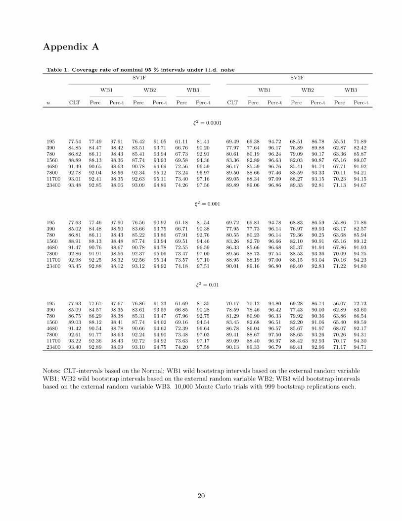
Table 1 gives the actual rates of 95% confidence intervals of integrated volatility for the SV1F
and the SV2F models, respectively, computed over 10,000 replications. Results are presented for eight
different samples sizes: n = 23400, 11700, 7800, 4680, 1560, 780, 390 and 195, corresponding to “1-
second”, “2-second”, “3-second”, “5-second”, “15-second”, “30-second”, “1-minute” and “2-minute”
frequencies (this table also includes results for the bootstrap methods but those results will be discussed
later in Section 4.)
For the two models, all intervals tend to undercover. The degree of undercoverage is especially
large for smaller values of n, when sampling is not too frequent. The SV2F model exhibits overall
larger coverage distortions than the SV1F model, for all sample sizes. Results are not very sensitive
2The function s-exp is the usual exponential function with a linear growth function splined in at high values of itsargument: s-exp(x) = exp(x) if x ≤ x0 and s-exp(x) = exp(x0)√
x0−x20+x2if x > xo, with x0 = log(1.5).
10

to the noise magnitude.
3 The bootstrap
In this section we provide a bootstrap method for inference on integrated volatility based on the pre-
averaging approach of Podoslkij and Vetter (2009). Our proposal is to bootstrap the pre-averaged
returns Yj , j = 1, . . . , n/K. Because non-overlapping intervals are used, the pre-averaged returns
Yj are asymptotically uncorrelated, as n → ∞. In fact, we can show that they are one-dependent
(conditionally on X), i.e. Yj is independent of Ym whenever |m− j| > 1. Moreover, the amount of
dependence between two consecutive squared pre-averaged returns is very small and it is only due to
edge effects. Specifically, Cov(Y 2j , Y
2j+1
)= O
(1n2
)= o (1) as n→∞.
Since pre-averaged returns are asymptotically uncorrelated but possibly heteroskedastic (due to
the fact that volatility is time-varying) a wild bootstrap approach is appropriate. The wild bootstrap
method was introduced by Wu (1986), and further studied by Liu (1988) and Mammen (1993), in
the context of cross-section linear regression models subject to unconditional heteroskedasticity in
the error term. Goncalves and Meddahi (2009) applied the wild bootstrap method in the context of
realized volatility under no market microstructure noise. Our approach here follows Goncalves and
Meddahi (2009), but instead of bootstrapping the 1n -horizon raw returns ri, we propose to bootstrap
the pre-averaged returns Yj .
The bootstrap pseudo-data is given by
Y ∗j = Yj · vj , j = 1, . . . , n/K,
where the external random variable vj is an i.i.d. random variable independent of the data and
whose moments are given by µ∗q ≡ E∗ |vj |q. As usual in the bootstrap literature, P ∗ (E∗ and V ar∗)
denotes the probability measure (expected value and variance) induced by the bootstrap resampling,
conditional on a realization of the original time series. In addition, for a sequence of bootstrap statistics
Z∗n, we write Z∗n = oP ∗ (1) in probability, or Z∗n →P ∗ 0, as n → ∞, in probability, if for any ε > 0,
δ > 0, limn→∞ P [P ∗ (|Z∗n| > δ) > ε] = 0. Similarly, we write Z∗n = OP ∗ (1) as n → ∞, in probability
if for all ε > 0 there exists a Mε <∞ such that limn→∞ P [P ∗ (|Z∗n| > Mε) > ε] = 0. Finally, we write
Z∗n →d∗ Z as n → ∞, in probability, if conditional on the sample, Z∗n weakly converges to Z under
P ∗, for all samples contained in a set with probability P converging to one.
The bootstrap pre-averaged realized volatility estimator is given by
PRV ∗n =c1c2ν1
n/K∑j=1
Y ∗2j .
Although the pre-averaged realized volatility estimator PRVn contains a bias correction term, we do
not consider bias correction in the bootstrap world. The reason is twofold. First, our goal is not
to estimate consistently the integrated volatility using the bootstrap. Instead, our goal is to use the
11

bootstrap to approximate the distribution of statistics based on PRVn, for instance we would like to
approximate the distribution of the t-statistic Tn defined in the previous section. We can easily show
that
E∗ (PRV ∗n ) = µ∗2c1c2ν1
n/K∑j=1
Y 2j .
This is a biased estimator of integrated volatility, but we can correctly center our bootstrap statistics
using this theoretical bootstrap mean. Since the bias correction term does not affect the variance
of the pre-averaging estimator, as long as the bootstrap method is able to consistently estimate this
variance, no bias correction is needed in the bootstrap world. The second reason why we do not consider
bootstrap bias correction is that the bootstrap bias correction term would involve the bootstrap highest
frequency returns r∗i , which are not available under our proposed method.
We can show that
V ar∗(n1/4PRV ∗n
)=(µ∗4 − µ∗22
) c21c22ν21
√n
n/K∑j=1
∣∣Yj∣∣4︸ ︷︷ ︸≡ 3
2Vn
.
It follows then that a sufficient condition for the bootstrap to provide a consistent estimator of the
conditional variance of n1/4PRVn is that µ∗4 − µ∗22 = 23 . Under this condition, the bootstrap can be
used to approximate the quantiles of the distribution of the root
n1/4(PRVn −
∫ 1
0σ2sds
),
thus justifying the construction of bootstrap percentile confidence intervals.
These results are summarized in the following theorem.
Theorem 3.1. Suppose Assumption 1 holds and let K and L satisfy the conditions (4) and (5),
respectively. Suppose thatY ∗j = Yj · vj : j = 1, . . . , n/K
, where vj ∼ i.i.d. such that for any δ > 0,
µ∗2(2+δ) = E∗ |vj |2(2+δ) <∞. If µ∗4 − (µ∗2)2 = 2
3 , then as n→∞,
(1) V ∗n ≡ V ar∗(n1/4PRV ∗n
) P→ V ≡ 2c21c22
ν21
∫ 10
(ν1σ
2s + ν2ω
2)2ds.
(2) supx∈R
∣∣∣P ∗ (n1/4 (PRV ∗n − E∗ (PRV ∗n )) ≤ x)− P
(n1/4
(PRVn −
∫ 10 σ
2sds))∣∣∣ P→ 0.
An example of a random variable that satisfies the condition µ∗4 − µ∗22 = 23 is
vj ∼ i.i.d. N(
0,√
3/3).
Theorem 3.1 justifies using the wild bootstrap to construct bootstrap percentile intervals for inte-
grated volatility. Specifically, a 100 (1− α) % symmetric bootstrap percentile interval for integrated
volatility based on the bootstrap is given by
IC∗perc,1−α =(PRVn − n−1/4p∗1−α, PRVn + n−1/4p∗1−α
), (7)
12

where p∗1−α is the 1− α quantile of the bootstrap distribution of∣∣n1/4 (PRV ∗n − E∗ (PRV ∗n ))
∣∣ .Bootstrap percentile intervals do not promise asymptotic refinements. Next, we propose a con-
sistent bootstrap variance estimator that allows us to form bootstrap percentile-t intervals. More
specifically, we can show that the following bootstrap variance estimator consistently estimates V ∗n for
any choice of the external random variable vj :
V ∗n =µ∗4 − µ∗22
µ∗4
c21c22
ν21n1/2
n/K∑j=1
Y ∗4j .
Our proposal is to use this estimator to construct a bootstrap studentized statistic,
T ∗n ≡n1/4 (PRV ∗n − E∗ (PRV ∗n ))√
V ∗n
,
the bootstrap analogue of Tn.
Theorem 3.2. Suppose Assumption 1 holds such that for any δ > 0, E |εt|2(8+δ) <∞, and let K and
L satisfy the conditions (4) and (5), respectively. Suppose thatY ∗j = Yj · vj : j = 1, . . . , n/K
, where
vj ∼ i.i.d. such that µ∗8 = E∗ |vj |8 <∞. It follows that as n→∞, supx∈R |P ∗ (T ∗n ≤ x)− P (Tn ≤ x)| P→0.
Theorem 3.2 justifies constructing bootstrap percentile-t intervals. In particular, a 100 (1− α) %
symmetric bootstrap percentile-t interval for integrated volatility is given by
IC∗perc−t,1−α =
(PRVn − q∗1−αn−1/4
√Vn, PRVn + q∗1−αn
−1/4√Vn
), (8)
where q∗1−α is the (1− α)-quantile of the bootstrap distribution of |T ∗n |. The first order asymptotic
validity of the bootstrap requires a strenthening of the moment condition on εt when applied to the
feasible statistic Tn.
4 Monte Carlo results for the bootstrap
In this section, we compare the finite sample performance of the bootstrap with the first order asymp-
totic theory for confidence intervals of integrated volatility in the case of i.i.d. and autocorrelated
market microstructure noise. In our simulations, bootstrap intervals use 999 bootstrap replications
for each of the 10,000 Monte Carlo replications.
To generate the bootstrap data we use three different external random variables.
WB1 vj ∼ i.i.d. N(0,√
3/3), implying that µ∗2 =
√3/3 and µ∗4 = 1.
WB2 A two point distribution vj ∼ i.i.d. such that:
vj =
(23
)1/4 −1+√52 , with prob p =
√5−12√5(
23
)1/4 −1−√52 , with prob 1− p =
√5+12√5
,
13

for which µ∗2 = 2√
2/3 and µ∗4 = 10/3.
WB3 The two point distribution proposed by Goncalves and Meddahi (2009), where vj ∼ i.i.d. such
that:
vj =
15
√31 +
√186, with prob p = 1
2 −3√186
−15
√31−
√186, with prob 1− p
,
for which we have µ∗2 = 1 and µ∗4 = 31/25.
The condition µ∗4− (µ∗2)2 = 2
3 is satisfied for the first two choices (WB1 and WB2) but not for WB3.
The implication is that WB1 and WB2 are valid for percentile intervals but not WB3. Note however
that all three choices of vj are asymptotically valid when used to construct bootstrap percentile-t
intervals.
4.1 i.i.d. noise
In this subsection, we simulate results for the case of i.i.d. market microstructure noise, following
the same data generating process as in Section 2.4. We consider bootstrap percentile and bootstrap
percentile-t intervals, computed at the 95% level using (7) and (8), respectively. Table 1 shows the
actual coverage probability rates of nominal 95% symmetric bootstrap intervals for integrated volatility
based on WB1, WB2 and WB3 for each of the two models (SV1F and SV2F). Results based on the
asymptotic normal distribution are also included (under the label CLT). As already discussed in
Section 2.4, results are not very sensitive to the choice of ξ2 and distortions are larger (both based on
asymptotic theory and on the bootstrap) for the SV2F than for the SV1F model. These trends are
also present for the bootstrap.
Starting with the bootstrap percentile intervals, we see that these are close to the CLT-based
intervals for WB1 and WB2 (when the condition µ∗4− (µ∗2)2 = 2
3 is satisfied) whereas coverage rates
for percentile intervals based on WB3 are systematically much lower than 95% even for the largest
sample sizes. This confirms the theoretical prediction of asymptotic invalidity for these intervals.
The results also confirm that the bootstrap percentile intervals do not outperform the asymptotic
theory-based intervals. Nevertheless, choosing vj to match the variance of the pre-averaging estimator
may result in better percentile-t intervals, as a comparison of the different bootstrap methods shows
for this type of intervals. Specifically, although WB2 and WB3 both undercover for smaller sample
sizes, WB2 outperforms WB3 significantly for the smaller samples sizes. For instance, for SV1F, when
ξ2 = 0.0001, WB3 covers IV 81.41% of the time when n = 195 whereas WB2 does so 91.05%. These
rates decrease to 71.89% and 86.78% for the SV2F model, respectively. In contrast, the WB1 method
covers IV with a rate equal to 97.91% for SV1F and 94.72% for SV2F, when n = 195. In general,
the results show that percentile-t intervals based on WB1 are too conservative, yielding coverage rates
larger than 95%, especially for the SV1F model. WB2 intervals tend to be closer to the desired nominal
14
level than the WB3 method, without being conservative. Overall, the results suggest that the choice
of vj is important in finite samples.
In order to gain further insight into why the different choices of vj matter in finite samples, we
computed the first four cumulants of Tn and of its bootstrap analogue T ∗n . The results are presented
in Table 2, which also reports the coverage rates of symmetric intervals based on these studentized
statistics. Results are only given for ξ2 = 0.01. For Tn, we report the mean, the standard error, the
excess skewness and the excess kurtosis across the 10,000 simulations. For T ∗n , the numbers correspond
to the average value (across the 10,000 simulations) of the bootstrap mean, standard error, excess
skewness and excess kurtosis computed for each simulation across the 999 bootstrap replications.
Starting with Tn, the results show that this statistic is centered at a negative value across the
different sample sizes. The negative bias decreases as n increases, but it can be quite large when
n is small. Since the asymptotic normal distribution is centered at zero, it completely misses this
downward bias. We can also see that the finite sample distribution of Tn is more dispersed than the
N (0, 1) distribution (its standard error is larger than 1), and that it is strongly negatively skewed (the
excess skewness is very negative) and fat-tailed (the excess kurtosis is positive). All these features
explain the undercoverage of the CLT approach. In contrast, the bootstrap cumulants of T ∗n replicate
to a better degree the finite sample patterns of the four cumulants of Tn depending on the choice of
vj . Specifically, we can see that the three choices of vj typically induce a negative bias as well as
negative excess skewness and positive excess kurtosis (an exception is WB3 for the smaller sample
sizes). Nevertheless, WB1 implies too strong a correction. For instance, the bias of T ∗n is more
negative than it should be on average as well as its excess skewness. This means that the bootstrap
distribution of T ∗n is on average to the left of the finite sample distribution of Tn, resulting in too
large a critical value, which explains the overcoverage problem noted in Table 1. In contrast, for the
smaller sample sizes, WB2 and WB3 imply too little a correction in terms of the bias, which implies
that these bootstrap distributions are on average centered to the right of the true distribution of Tn.
This contributes to too small a critical value and to some undercoverage.
Overall, the results suggest that WB3 does a poorer job at capturing the first four cumulants than
WB2, especially for the smaller sample sizes. This suggests that the optimal choice of vj proposed
by Goncalves and Meddahi (2009) in the context of realized volatility without market microstructure
noise is no longer optimal in the context of pre-averaging realized volatility. The presence of the bias
correction term in the definition of PRVn implies that the Edgeworth expansions derived in Goncalves
and Meddahi (2009) do not apply in the pre-averaging approach considered here. Thus, although bias
correction does not have an impact to first order on the asymptotic variance of PRVn, it likely has
an impact on the higher order cumulants, as our Monte Carlo simulation results suggest. Deriving
the optimal choice of the external random variable in this context is an interesting research question
which we will consider elsewhere.
15

4.2 Autocorrelated noise
In a second set of experiments, we look at the case where the market microstructure noise is autocor-
related. Recently, Hautsch and Podolskij (2013) have formally developed the theory of pre-averaging
estimators in this case. While Hautsch and Podolskij’s (2013) results apply specifically to the over-
lapping pre-averaging approach, the same bias correction can also be used for the non-overlapping
pre-averaged estimator considered here. Indeed, as Podolskij and Vetter (2009) discuss in their Sec-
tion 3.1.3, relaxing the i.i.d. noise assumption to allow for q−dependence implies that their main
consistency result for non-overlapping pre-averaged estimators (cf. their Theorem 1) still holds. The
key difference is that the limit now depends on the higher order autocorrelations of the noise pro-
cess instead of depending on ω2 = V ar (εi) (in particular, ω2 is replaced by the long run variance
ρ2 = ρ (0) + 2∑q
k=1 ρ (k), where ρ (k) = Cov (ε1, ε1+k) , and q is the order of dependence of the noise
process (εi)i≥0). The main implication is that the bias correction for pre-averaged realized volatility
must depend on an estimator of ρ2. Hautsch and Podolskij’s (2013) discuss an estimator of ρ2 given
by
ρ2n = ρn (0) + 2
q∑k=1
ρn (k) ,
where ρn (0) , . . . , ρn (q) are obtained by a simple recursion,
ρn (q) = −γn (q + 1) ,
ρn (q − 1) = −γn (q) + 2ρn (q) ,
ρn (q − 2) = −γn (q − 1) + 2ρn (q − 1)− ρn (q) ,
where γn (k) =1
n
n∑i=1
riri+k, k = 0, . . . , q + 1.
This implies the following consistent estimator of integrated volatility under a q-dependent autocor-
related noise process:
PRV an =
c1c2ν1
n/K∑j=1
Y 2j︸ ︷︷ ︸
RV -like estimator
− ν2ν1ρ2n︸ ︷︷ ︸
new bias correction term
. (9)
As it turns out, while the asymptotic variance of PRV an depends on the long run variance of the noise,
the same variance estimator as the one used under i.i.d. noise (Vn in our notation) can still be used
in the autocorrelated case (this is again a consequence of the fact that Podolskij and Vetter’s (2009)
Theorem 1 holds when εi is autocorrelated). This fact leads us to conjecture that the wild bootstrap
is valid when applied to the new bias adjusted pre-averaged volatility estimator under autocorrelated
noise. Although we do not provide a formal proof of this result, in this section we explore the finite
sample properties of the wild bootstrap under autocorrelation in εi.
In particular, we follow Kalnina (2011) and let the market microstructure noise be generated as
16
an MA(1) process (for a given frequency of the observations):
ε in
= u in
+ θu i−1n, u i
n∼ i.i.d.N
(0,
ω2
1 + θ2
), (10)
so that V ar (ε) = ω2. We set θ = −0.5 and chose ω2 as in the i.i.d. case discussed above, i.e. we let
ω2 = ξ2√∫ 1
0 σ4sds. Because the results are not very sensitive to the value of ξ2, we only report results
for ξ2 = 0.01.
Our aim here is to evaluate by Monte Carlo simulation the performance of the wild bootstrap when
applied to the statistic that relies on the new bias correction of Hautsh and Podoskij (2013), which is
robust to noise autocorrelation. We consider three types of intervals as before (intervals based on the
asymptotic normal distribution, bootstrap percentile and bootstrap percentile-t intervals), computed
at the 95% level. More specifically, we consider the following intervals,
ICFeas,0.95 =
(PRV a
n − 1.96n−1/4√Vn, PRV
an + 1.96n−1/4
√Vn
), (11)
IC∗perc,0.95 =(PRV a
n − n−1/4p∗0.95, PRV an + n−1/4p∗0.95
), and (12)
IC∗perc−t,0.95 =
(PRV a
n − q∗0.95n−1/4√Vn, PRV
an + q∗0.95n
−1/4√Vn
). (13)
Whereas (11) corresponds to an asymptotic theory-based interval, (12) and (13) correspond to boot-
strap percentile and percentile-t intervals, respectively. Note that in the latter case, the bootstrap
quantiles (p∗0.95 and q∗0.95) are computed exactly as in the i.i.d. case (they are based on the absolute
value of n1/4 (PRV ∗n − E∗ (PRV ∗n )) and of T ∗n , whose form is unaffected by the new bias adjustment
used in PRV an ).
Table 3 contains the results. Two sets of results are presented. First, we present results for intervals
based on PRVn, the non-robust pre-averaged estimator discussed for the i.i.d. case (top part of the
table). Then, we present results for intervals based on PRV an , the robust estimator based on the new
bias correction of Hautsch and Podolskij (2013) (bottom part). The results show that intervals based
on PRVn are more distorted when there is autocorrelation in εi than otherwise. The main reason for
the distortions is the fact that PRVn is not correctly centered under autocorrelation. For instance, for
the SV1F model, when n = 195, the CLT-based interval has a coverage probability equal to 75.58%
under autocorrelated noise whereas its coverage rate (from Table 1) is equal to 77.93% under i.i.d.
noise. Although the difference is not very large for the smaller sample sizes, it gets much bigger for
larger values of n. For n = 23, 400, these rates equal 89.33% and 93.4%, respectively. Thus, the
problem does not disappear with increasing sample sizes. The differences between the two intervals
are larger for the SV2F model. For instance, the rates for n = 195 are equal to 70.17% under i.i.d.
noise and equal to 66.13% under MA(1) errors. For n = 23, 400, they are equal to 90.13% and 83.86%,
respectively.
However, if we rely on PRV an as a point estimator of integrated volatility, the corresponding
17

intervals (both asymptotic and bootstrap) are better centered and the distortions are smaller and
closer to their values under the i.i.d. noise. For instance, the CLT-based intervals for SV1F now have
coverage rates equal to 78.51% and 93.89% when n = 195 and n = 23, 400, respectively. A similar
pattern is observed for the SV2F model, although the rates are overall smaller (they are equal to
69.62% and 90.15%, respectively).
When the wild bootstrap method WB2 is used to compute critical values for the t-test based on
PRVn and the error is MA(1), coverage rates are usually smaller than those obtained when the noise
is i.i.d (and therefore distortions are larger). As for the CLT-based intervals, the larger differences
occur for the larger sample sizes (for instance, for the SV1F model, the rate is equal to 91.44% under
MA(1) error when n = 23, 400, whereas it is equal to 94.75% under i.i.d. error). For the smaller
sample sizes, the difference in coverage probability between the two types of errors is much smaller. It
is almost negligible for the SV1F model, although it is slighly larger for the SV2F model. As for the
CLT-based intervals, using the wild bootstrap to compute critical values for the t-statistic based on
PRV an essentially eliminates the difference in coverage probabilities observed between the i.i.d. and
the MA(1) errors. When compared to WB1 and WB3, the wild bootstrap intervals based on WB2
seem to do best overall. In particular, the comparison between the three methods is similar to what
we observed for the i.i.d. noise case when they are used to compute critical values for the t-statistic
based on PRV an .
In summary, the results in Table 3 show that under autocorrelated noise the statistic based on the
bias correction of Hautsch and Podolskij (2013) works well and that the coverage rates of 95% nominal
level intervals based on either the asymptotic mixed Gaussian distribution or the wild bootstrap
proposed in this paper are similar to those obtained under i.i.d. noise.
5 Empirical results
As a brief illustration, in this section we implement the proposed wild bootstrap method on real high
frequency data, and compare it to the existing feasible asymptotic procedure of Podolskij and Vetter
(2009). The data consists of transaction log prices of General Electric (GE) shares carried out on
the New York Stock Exchange (NYSE) in December 2011. For each day, we consider data from the
regular exchange opening hours from time stamped between 9:30 a.m. until 4 p.m. Our procedure for
cleaning the data is exactly identical to that used by Barndorff-Nielsen et al. (2008).
We implement the pre-averaged realized volatility estimator of Podolskij and Vetter (2009) (pos-
sibly corrected for autocorrelation in the noise) on returns recorded every S transactions, where S is
selected each day so that there are approximately 1493 observations a day. This means that on average
these returns are recorded roughly every 15 seconds. Table 4 in the Appendix provides the number
of transactions per day, the sample size for the pre-averaged returns, and the dependent-noise robust
version of the pre-averaged realized volatility estimator using (9) (for q = 0, 1 and 2). We also report
18
the optimal value of q (the number of non-vanishing covariances) using the decision rule proposed
by Hautsch and Podolskij (2013). The pre-averaged realized volatility estimator is implemented with
c2 = 1.6 and c1 = 1. As the results in Table 4 show, there are some days on our sample for which
there is evidence of significant serial correlation in the noise process.
We consider bootstrap percentile-t intervals, computed at the 95% level using (13), where vj
is generated using WB2 (our best choice according to the Monte Carlo simulations). The results
are displayed in Figure 1 in terms of daily 95% confidence intervals (CIs) for integrated volatility.
Two types of intervals are presented: our proposed wild bootstrap method and the existing feasible
asymptotic procedure Podolskij and Vetter (2009) (corrected by the Hautsch and Podolskij (2013) bias
formula when q > 0). In particular, the pre-averaged realized volatility estimate is computed using
(9) with the optimal value of q, and is in the center of both confidence intervals by construction.
The confidence intervals for integrated volatility based on the bootstrap method are usually wider
than the confidence intervals using the feasible asymptotic theory. Nevertheless, as our Monte Carlo
simulations showed, the latter typically have undercoverage problems whereas the bootstrap intervals
have coverage rates closer to the desired level. Therefore, if the goal is to control the coverage prob-
ability, shorter intervals are not necessarily better. The figure also shows a lot of variability in the
daily estimate of integrated volatility.
6 Conclusion
In this paper, we propose the wild bootstrap as a method of inference for integrated volatility in the
context of the pre-averaged realized volatility estimator proposed by Podolskij and Vetter (2009). The
wild bootstrap is motivated by the fact that non-overlapped pre-averaged returns are asymptotically
uncorrelated but possibly heteroskedastic (in the context of stochastic volatility models). We provide
a set of conditions under which this method is asymptotically valid to first order. Both percentile and
percentile-t bootstrap intervals are considered. Our Monte Carlo simulations show that the bootstrap
can improve upon the mixed Gaussian inference derived by Podolskij and Vetter (2009) provided we
choose the external random variable appropriately.
An important question for future research is the optimal choice of the external random variable
in this context. This is not an easy question because it requires developing Edgeworth expansions
for the statistics of interest in the original sample and the bootstrap samples. Since the pre-averaged
realized volatility estimator depends on a bias correction term, its Edgeworth expansion will reflect
the contribution of this term at higher orders and render the analysis rather complex. We plan on
investigating this issue in future work.
19
Appendix A
Table 1. Coverage rate of nominal 95 % intervals under i.i.d. noise
SV1F SV2F—————————————————————————– —————————————————————————–
WB1 WB2 WB3 WB1 WB2 WB3—————— —————— —————— —————— —————— ——————
n CLT Perc Perc-t Perc Perc-t Perc Perc-t CLT Perc Perc-t Perc Perc-t Perc Perc-t
ξ2 = 0.0001
195 77.54 77.49 97.91 76.42 91.05 61.11 81.41 69.49 69.38 94.72 68.51 86.78 55.51 71.89390 84.85 84.47 98.42 83.51 93.71 66.76 90.20 77.97 77.64 96.17 76.89 89.88 62.87 82.42780 86.82 86.11 98.43 85.41 93.94 67.73 92.91 80.61 80.19 96.24 79.09 90.17 63.36 85.871560 88.89 88.13 98.36 87.74 93.93 69.58 94.36 83.36 82.89 96.63 82.03 90.87 65.16 89.074680 91.49 90.65 98.63 90.78 94.69 72.56 96.59 86.17 85.59 96.76 85.41 91.74 67.71 91.927800 92.78 92.04 98.56 92.34 95.12 73.24 96.97 89.50 88.66 97.46 88.59 93.33 70.11 94.2111700 93.01 92.41 98.35 92.63 95.11 73.40 97.16 89.05 88.34 97.09 88.27 93.15 70.23 94.1523400 93.48 92.85 98.06 93.09 94.89 74.26 97.56 89.89 89.06 96.86 89.33 92.81 71.13 94.67
ξ2 = 0.001
195 77.63 77.46 97.90 76.56 90.92 61.18 81.54 69.72 69.81 94.78 68.83 86.59 55.86 71.86390 85.02 84.48 98.50 83.66 93.75 66.71 90.38 77.95 77.73 96.14 76.97 89.93 63.17 82.57780 86.81 86.11 98.43 85.22 93.86 67.91 92.76 80.55 80.23 96.14 79.36 90.25 63.68 85.941560 88.91 88.13 98.48 87.74 93.94 69.51 94.46 83.26 82.70 96.66 82.10 90.91 65.16 89.124680 91.47 90.76 98.67 90.78 94.78 72.55 96.59 86.33 85.66 96.68 85.37 91.94 67.86 91.937800 92.86 91.91 98.56 92.37 95.06 73.47 97.00 89.56 88.73 97.54 88.53 93.36 70.09 94.2511700 92.98 92.25 98.32 92.56 95.14 73.57 97.10 88.95 88.19 97.00 88.15 93.04 70.16 94.2323400 93.45 92.88 98.12 93.12 94.92 74.18 97.51 90.01 89.16 96.80 89.40 92.83 71.22 94.80
ξ2 = 0.01
195 77.93 77.67 97.67 76.86 91.23 61.69 81.35 70.17 70.12 94.80 69.28 86.74 56.07 72.73390 85.09 84.57 98.35 83.61 93.59 66.85 90.28 78.59 78.46 96.42 77.43 90.00 62.89 83.60780 86.75 86.29 98.38 85.31 93.47 67.96 92.75 81.29 80.90 96.33 79.92 90.36 63.86 86.541560 89.03 88.12 98.41 87.74 94.02 69.16 94.54 83.45 82.68 96.51 82.20 91.06 65.40 89.594680 91.42 90.54 98.78 90.66 94.62 72.39 96.64 86.78 86.04 96.57 85.67 91.97 68.07 92.177800 92.61 91.77 98.63 92.24 94.90 73.48 97.03 89.41 88.67 97.50 88.65 93.26 70.26 94.3111700 93.22 92.36 98.43 92.72 94.92 73.63 97.17 89.09 88.40 96.97 88.42 92.93 70.17 94.3023400 93.40 92.89 98.09 93.10 94.75 74.20 97.58 90.13 89.33 96.79 89.41 92.96 71.17 94.71
Notes: CLT-intervals based on the Normal; WB1 wild bootstrap intervals based on the external random variableWB1; WB2 wild bootstrap intervals based on the external random variable WB2; WB3 wild bootstrap intervalsbased on the external random variable WB3. 10,000 Monte Carlo trials with 999 bootstrap replications each.
20

Table 2. Summary results for the stutentized statistic Tn and its bootstrap analogue T ∗nSV1F SV2F
ξ2 = 0.01 Tn T ∗WB1n T ∗WB2
n T ∗WB3n Tn T ∗WB1
n T ∗WB2n T ∗WB3
n
n = 195Mean -1.109 -1.802 -0.552 -0.413 -1.798 -2.319 -0.752 -0.440Standard error 2.356 4.526 2.135 1.298 3.921 5.867 2.466 1.264Excess Skewness -3.717 -5.751 -3.024 -0.009 -6.000 -6.041 -2.724 0.158Excess Kurtosis 29.279 65.763 14.765 -1.206 72.426 71.078 11.29 -1.255
Cov two-sided 77.93 97.67 91.23 81.35 70.17 94.8 86.74 72.73
n = 390Mean -0.594 -1.275 -0.393 -0.373 -0.997 -1.676 -0.590 -0.410Standard error 1.661 2.969 1.755 1.317 2.325 3.776 2.119 1.283Excess Skewness -2.454 -3.940 -2.685 -0.169 -3.235 -4.218 -2.591 0.022Excess Kurtosis 11.775 31.511 12.71 -0.991 18.615 35.287 10.775 -1.13
Cov two-sided 85.09 98.35 93.59 90.28 78.59 96.42 90.00 83.60
n = 780Mean -0.519 -0.991 -0.297 -0.338 -0.850 -1.342 -0.482 -0.384Standard error 1.464 2.304 1.517 1.323 1.982 2.924 1.884 1.293Excess Skewness -1.973 -2.974 -2.235 -0.279 -2.620 -3.306 -2.391 -0.077Excess Kurtosis 8.798 17.221 9.053 -0.767 12.026 21.371 9.370 -1.005
Cov two-sided 86.75 98.38 93.47 92.75 81.29 96.33 90.36 86.54
n = 1560Mean -0.409 -0.788 -0.228 -0.299 -0.669 -1.094 -0.395 -0.357Standard error 1.297 1.909 1.353 1.323 1.704 2.389 1.690 1.300Excess Skewness -1.369 -2.381 -1.829 -0.366 -2.203 -2.672 -2.144 -0.166Excess Kurtosis 3.714 10.773 6.193 -0.519 9.133 13.287 7.579 -0.858
Cov two-sided 89.03 98.41 94.02 94.54 83.45 96.51 91.06 89.59
n = 23400Mean -0.191 -0.375 -0.095 -0.170 -0.334 -0.560 -0.183 -0.247Standard error 1.064 1.277 1.085 1.281 1.225 1.490 1.247 1.295Excess Skewness -0.592 -1.226 -0.859 -0.419 -1.117 -1.504 -1.331 -0.364Excess Kurtosis 0.599 2.611 1.357 0.066 2.518 3.794 3.053 -0.298
Cov two-sided 93.40 98.09 94.75 97.58 90.13 96.79 92.96 94.71
Notes: Tn studentized statistic; T ∗WB1n studentized wild bootstrap statistic based on WB1; T ∗WB2
n studentizedwild bootstrap statistic based on WB2; T ∗WB3
n studentized wild bootstrap statistic based on WB3. 10,000Monte Carlo trials with 999 bootstrap replications each.
21

Table 3. Coverage rate of nominal 95 % intervals under autocorrelated noise, θ = −0.5, ξ2 = 0.01
SV1F SV2F—————————————————————————– —————————————————————————–
WB1 WB2 WB3 WB1 WB2 WB3—————— —————— —————— —————— —————— ——————
n CLT Perc Perc-t Perc Perc-t Perc Perc-t CLT Perc Perc-t Perc Perc-t Perc Perc-t
ˆBias = ν2ν1
∑ni=1 r
2i
2n
195 75.58 75.33 97.27 74.53 89.83 58.84 79.22 66.13 66.01 93.89 65.06 84.54 51.75 68.38390 82.98 82.69 98.11 81.46 92.07 64.67 88.69 74.10 73.86 95.52 73.10 87.97 60.09 79.18780 84.37 83.72 97.91 82.76 92.33 65.83 90.79 76.16 75.78 95.44 74.97 88.22 59.59 82.451560 86.26 85.57 98.03 85.00 92.59 66.59 93.19 78.60 78.09 95.47 77.23 88.04 61.72 85.464680 88.03 87.00 97.32 87.13 91.95 69.58 94.12 82.41 81.51 95.34 81.30 89.37 64.83 89.337800 90.34 89.52 98.03 89.69 93.08 71.68 95.85 84.57 83.80 96.44 83.40 90.78 66.58 91.6211700 90.15 89.43 97.26 89.64 92.33 70.85 95.47 84.74 83.85 95.87 83.66 90.05 65.43 91.3623400 89.33 88.65 96.51 89.03 91.44 69.67 95.34 83.86 82.98 94.63 83.09 88.62 65.34 91.14
ˆBias = ν2ν1ρ2n
195 78.51 78.31 97.62 77.29 91.05 61.84 81.94 69.62 69.71 94.81 68.47 86.44 55.21 71.83390 85.45 85.19 98.48 83.92 93.36 66.74 90.73 78.03 78.02 96.46 76.86 89.92 62.98 82.47780 87.15 86.55 98.44 85.73 93.62 68.40 92.65 80.18 79.91 96.45 78.86 90.53 63.28 85.841560 89.60 88.88 98.61 88.37 94.57 69.33 95.15 82.81 82.31 96.80 81.66 90.52 65.63 88.654680 91.42 90.64 98.26 90.69 94.26 72.86 96.13 87.31 86.58 96.80 86.28 92.40 69.08 92.447800 93.26 92.68 98.88 92.75 95.54 74.52 97.64 89.69 88.96 97.69 88.83 94.03 70.87 94.8911700 93.44 92.70 98.36 92.99 95.15 74.74 97.35 89.87 89.08 97.56 89.10 93.60 70.83 94.9923400 93.89 93.23 98.19 93.56 95.10 74.65 97.48 90.15 89.35 97.19 89.51 93.16 71.35 95.28
Notes: CLT-intervals based on the Normal; WB1 wild bootstrap intervals based on the external random variableWB1; WB2 wild bootstrap intervals based on the external random variable WB2; WB3 wild bootstrap intervals
based on the external random variable WB3; ˆBias = ν2ν1
∑ni=1 r
2i
2n is a consistent estimator of the bias term in
PRVn under i.i.d. noise; ˆBias = ν2ν1ρ2n is a consistent estimator of the bias term in PRV an under autocorrelated
noise. 10,000 Monte Carlo trials with 999 bootstrap replications each.
22

Table 4: Summary statistics
Days Trans n S PRV an · 103 q∗ PRV an · 103————————– ————q = 0 q = 1 q = 2 q = q∗
1 Dec 11924 1491 8 0.406 0.408 0.408 1 0.4082 Dec 11681 1461 8 0.351 0.353 0.353 0 0.3515 Dec 10538 1506 7 0.382 0.383 0.382 0 0.3826 Dec 12959 1440 9 0.256 0.347 0.565 5 0.6657 Dec 11360 1420 8 0.377 0.398 0.402 5 0.5098 Dec 10064 1438 7 0.348 0.349 0.348 0 0.3489 Dec 12120 1515 8 0.387 0.490 0.564 5 0.60112 Dec 12082 1511 8 0.374 0.437 0.561 5 0.59813 Dec 10379 1483 7 0.162 0.187 0.220 5 0.30514 Dec 12616 1577 8 0.358 0.463 0.584 5 0.59515 Dec 10869 1553 7 0.269 0.269 0.270 0 0.26916 Dec 12265 1534 8 0.365 0.367 0.367 0 0.36519 Dec 11119 1589 7 0.368 0.369 0.369 0 0.36820 Dec 12623 1578 8 0.377 0.378 0.378 0 0.37721 Dec 13270 1475 9 0.390 0.392 0.392 0 0.39022 Dec 14765 1476 10 0.460 0.461 0.461 0 0.46023 Dec 10970 1568 7 0.347 0.348 0.348 0 0.34727 Dec 10206 1458 7 0.364 0.365 0.365 0 0.36428 Dec 9580 1597 6 0.488 0.489 0.489 0 0.48829 Dec 10876 1554 7 0.254 0.255 0.255 0 0.25430 Dec 9839 1406 7 0.264 0.421 0.438 5 0.528
“Trans” denotes the number of transactions, n is the sample size used to calculate the pre-averaged realizedvolatility, we have sampled every Sth transaction price, so the period over which returns are calculated is roughly15 seconds. PRV an is the dependent-noise robust version of the pre-averaged realized volatility estimator, q isthe order of autocorrelation, q∗ is the optimal value of q selected using the decision rule proposed by Hautschand Podolskij (2013).
Figure 1: 95% Confidence Intervals (CI’s) for the daily IV, for each regular exchange opening days in December
2011, calculated using the asymptotic theory of Podolskij and Vetter (2009) (CI’s with bars), and the
wild bootstrap method using WB2 as external random variable (CI’s with lines). The pre-averaging
realized volatility estimator is the middle of all CI’s by construction. Days on the x-axis.
23

Appendix B
Proof of Theorem 3.1. For part (1), given that Yj∗ =Yjvj , where vj are i.i.d. with µ∗q = E∗ |vj |q,
for any q > 0, we have that
V ∗n = V ar∗
n1/4 c1c2ν1
n/K∑j=1
Yj∗2
= V ar∗
n1/4 c1c2ν1
n/K∑j=1
Y 2j v
2j
=
(µ∗4 − (µ∗2)
2)c21c22ν21
n1/2n/K∑j=1
Y 4j = Vn
under the condition that µ∗4 − (µ∗2)2 = 2
3 . Thus,
V ∗nP→ V =
2c21c22
ν21
1∫0
(ν1σ
2u + ν2ω
2)2du,
by an application of Theorem 1 of Podolskij and Vetter (2009) (where we set r = 4 and l = 0).
For part (2), let S∗n =n/K∑j=1
z∗j , where z∗j = c1c2ν1n1/4
(Yj∗2 − E∗
(Yj∗2)) . Note that E∗
(z∗j
)= 0 and
that
V ar∗
n/K∑j=1
z∗j
= V ∗nP→ V,
by part (1). Moreover, since z∗1 , . . . , z∗n/K are conditionally independent, by the Berry-Esseen bound,
for some small δ > 0 and for some constant C > 0,
supx∈R
∣∣∣P ∗ (S∗n ≤ x)−Φ(x/√V)∣∣∣ ≤ C n/K∑
j=1
E∗∣∣z∗j ∣∣2+δ ,
which converges to zero in probability as n→∞. Indeed, we have that
n/K∑j=1
E∗∣∣z∗j ∣∣ 2+δ =
∣∣∣∣c1c2ν1∣∣∣∣2+δ n/K∑
j=1
E∗∣∣∣n1/4 (Y ∗2j − E∗ (Y ∗2j ))∣∣∣2+δ
≤ 2
∣∣∣∣c1c2ν1∣∣∣∣2+δ n (2+δ)
4
n/K∑j=1
E∗∣∣Y ∗2j ∣∣ 2+δ
≤ 2
∣∣∣∣c1c2ν1∣∣∣∣2+δ E∗ |v1|2(2+δ) n− δ4
n (1+δ)2
n/K∑j=1
∣∣Y 2j
∣∣ 2+δ= Op
(n−
δ4
)= op (1) ,
since E |v1| 2(2+δ) ≤ ∆ < ∞ by assumption, and given that by Theorem 1 of Podolskij and Vetter
(2009)
n(1+δ)
2
n/K∑j=1
∣∣Y j
∣∣2(2+δ) P→µ2(2+δ)
c1c2
1∫0
(ν1σ
2u + ν2ω
2)2+δ
du,
which is bounded since σ is an adapted cadlag spot volatility process and locally bounded away from
24
zero, and E(ε2t ) = ω2 < ∆ <∞.
Proof of Theorem 3.2 Given that Tnd→ N(0, 1) (cf. Corollary 1 of Podolskij and Vetter (2009), it
suffices to show that T ∗nd∗→ N(0, 1) in probability. Let
H∗n =n1/4 (PRV ∗n − E∗ (PRV ∗n ))√
V ∗n,
and note that
T ∗n = H∗n
√V ∗n
V ∗n,
where V ∗n is defined in the main text. Theorem 3.1 proved that H∗nd∗→ N(0, 1) in probability. Thus,
it suffices to show that V ∗n − V ∗nP ∗→ 0 in probability. In particular, we show that (1) Bias∗
(V ∗n
)= 0,
and (2) V ar∗(V ∗n
)P→ 0. It is easy to verify that (1) holds by the definition of V ∗n and V ∗n . To prove
(2), note that
V ar∗(V ∗n
)= E∗
(V ∗n − V ∗n
)2=
(µ∗4 − (µ∗2)
2
µ∗4
)2
nc21c
22
ν21E∗
n/K∑j=1
(Y
4jv
4j − µ∗4Y
4j
)2
=
(µ∗4 − (µ∗2)
2
µ∗4
)2
nc21c
22
ν21
n/K∑j=1
Y8jE∗ (v4j − µ∗4)2
=
(µ∗4 − (µ∗2)
2
µ∗4
)2 (µ∗8 − µ∗24
) c21c22ν21
n−12n
32
n/K∑j=1
Y8j
= OP
(n−
12
)= oP (1) ,
where we have used the independence of vj over j to justify the third equality and Theorem 1 of
Podolskij and Vetter (2009) (with r = 8 and l = 0) to justify the fact that n32
n/K∑j=1
Y8j = OP (1). This
requires strengthening the moment condition on ε by assuming that E |ε|2(8+ε) <∞.
References
[1] Bandi, F., and J. Russell (2008). “Microstructure noise, realized variance, and optimal sampling, ” Reviewof Economic Studies, 75(2), 339-369.
[2] Barndorff-Nielsen, O., P. Hansen, A. Lunde, and N. Shephard (2008). “Designing realised kernels to mea-sure the ex-post variation of equity prices in the presence of noise,” Econometrica, 76, 1481-1536.
[3] Barndorff-Nielsen, O.E., Hansen, P.R., Lunde, A., Shephard, N. (2009). “Realised kernels in practice:trades and quotes, ” Econometrics Journal 12, C1-C32.
[4] Buhlmann, P. and H. R. Kunsch (1995). “The blockwise bootstrap for general parameters of a stationarytime series,” Scandinavian Journal of Statistics, 22(1), 35-54.
[5] Christensen, K., S. Kinnebrock, and M. Podolskij (2010). “Pre-averaging estimators of the ex-post co-variance matrix in noisy diffusion models with non-synchronous data, ” Journal of Econometrics, 159,116-133.
[6] Diebold, F.X. and Strasser, G.H. (2012). “On the correlation structure of microstructure noise: a financialeconomic approach”, Review of Economics Studies, forthcoming.
25

[7] Goncalves, S. and N. Meddahi (2009). “Bootstrapping realized volatility,” Econometrica, 77(1), 283.306.
[8] Heston, S. (1993). “Closed-form solution for options with stochastic volatility with applications to bondsand currency options,” Review of Financial Studies, 6, 327-343.
[9] Hansen, P.R. and A. Lunde (2006). “Realized variance and market microstructure noise,”Journal of Busi-ness and Economics Statistics, 24, 127-161.
[10] Hautsch N., and Podolskij, M., (2013). “Pre-averaging based estimation of quadratic variation in thepresence of noise and jumps: Theory, Implementation, and Empirical Evidence,” Journal of Business andEconomic Statistics, 31(2), 165-183.
[11] Hounyo, U. , Goncalves, S., and N. Meddahi (2013). “Bootstrapping pre-averaged realized volatility undermarket microstructure noise,” manuscript.
[12] Huang, X., and G. Tauchen (2006). “The Relative Contribution of Jumps to Total Price Variance, ”Journal of Financial Econometrics, 3, 456–499.
[13] Jacod, J., Y. Li, P. Mykland, M. Podolskij, and M. Vetter (2009). “Microstructure noise in the continuouscase: the pre-averaging approach,” Stochastic Processes and Their Applications, 119, 2249-2276.
[14] Kalnina, I. (2011). “Subsampling high frequency data,” Journal of Econometrics, 161(2), 262-283.
[15] Kunsch, H.R. (1989). “The jackknife and the bootstrap for general stationary observations,” Annals ofStatistics 17, 1217-1241.
[16] Liu, R.Y. (1988). “Bootstrap procedure under some non-i.i.d. models,” Annals of Statistics 16, 1696-1708.
[17] Mammen, E. (1993). “Bootstrap and wild bootstrap for high dimensional linear models,” Annals of Statis-tics 21, 255-285.
[18] Podolskij, M., and M. Vetter (2009). “Estimation of volatility functionals in the simultaneous presence ofmicrostructure noise and jumps,” Bernoulli, 15(3), 634-658.
[19] Politis, D. N. and Romano, J. P. (1992). “A general resampling scheme for triangular arrays of α-mixingrandom variables,” Annals of Statistics 20, 1985-2007.
[20] Vetter, M. (2008). “Estimation methods in noisy diffusion models,” Ph.D. Thesis. Bochum University.
[21] Wu, C.F.J., (1986). “Jackknife, bootstrap and other resampling methods in regression analysis,” Annalsof Statistics 14, 1261-1295.
[22] Zhang, L, P.A. Mykland, and Y. Aıt-Sahalia (2005). “A tale of two time-scales: determining integratedvolatility with noisy high frequency data,” Journal of the American Statistical Association, 100, 1394-1411.
[23] Zhang, L., Mykland, P. and Y. Aıt-Sahalia, (2011). “Ultra high frequency volatility estimation with de-pendent microstructure noise,” Journal of Econometrics, 160, 160-165.
[24] Zhou, B. (1996). “High-Frequency Data and Volatility in Foreign-Exchange Rates,” Journal of Businessand Economic Statistics, 14, 45–52.
26