durmm: the delaware urban runoff management model · the delaware urban runoff management model ......
TRANSCRIPT
DURMM: THE DELAWARE URBAN RUNOFF
MANAGEMENT MODEL
A USERS MANUAL FOR DESIGNING GREEN TECHNOLOGY BMPs TO MINIMIZE STORMWATER IMPACTS FROM LAND
DEVELOPMENT
William C. Lucas
INTEGRATED LAND MANAGEMENT, INC.
Prepared For
Delaware Department of Natural Resources And Environmental Control
Division of Soil And Water Conservation
JANUARY 2004
DURMM Users Manual Preface
JANUARY 2004 i
TABLE OF CONTENTS
PAGE
PREFACE..……………………..…….…….……...………………….…………………..….. ii
CHAPTER 1 URBAN RUNOFF HYDROLOGY AND HYDRAULICS 1.1 DURMM MODEL OVERVIEW…..……………………..……..……..……..….…………. 1-1
1.2 DURMM LAND COVER/AREA INPUT..……………………..…….…….…….....……... 1-4
1.3 TIME OF CONCENTRATION- SHEET FLOW…………………….………..……..….... 1-4
1.4 TIME OF CONCENTRATION- OVERLAND SWALE FLOW……….……….………… 1-5
1.5 STORAGE ROUTING………………………………..……….……….……...…………… 1-6
CHAPTER 2 BMP POLLUTANT REMOVAL 2.1 RUNOFF POLLUTANT ROUTING…....…..….………………………………..…..……. 2-1
2.2 REDUCTION KINETICS………………………………………………………..…..……... 2-1
2.3 FILTER STRIP BMPS……………………………………………………………….…..... 2-2
2.4 BIOFILTRATION SWALE BMPS…………………………………………...…..……..... 2-3
2.5 BIORETENTION BMPS………………………………………………………………....... 2-4
2.6 INFILTRATION TRENCH BMPS…………………………..…...……….……..………… 2-6
CHAPTER 3 DURMM EXAMPLE- PRE-DEVELOPMENT CONDITIONS…….….…. 3-1
CHAPTER 4 DURMM EXAMPLE- POST-DEVELOPMENT CONDITIONS…...….... 4-1
LIST OF FIGURES
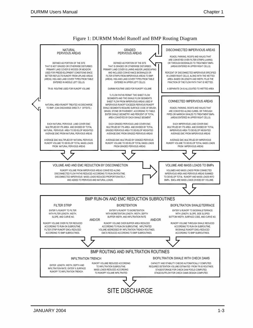
FIGURE 1: DURMM MODEL RUNOFF AND BMP ROUTING DIAGRAM……………….…… 1-3
FIGURE 2: EXAMPLE SITE- PRE-DEVELOPMENT CONDITIONS………………………...… 3-2
FIGURE 3: EXAMPLE SITE- POST-DEVELOPMENT CONDITIONS………………………… 4-2
APPENDICES APPENDIX A – USERS GUIDE
APPENDIX B – STEP BY STEP GUIDE

DURMM Users Manual Preface
JANUARY 2004 ii
PREFACE
This Manual is written as the companion document to “Green Technology: The Delaware
Urban Runoff Management Approach, a Technical Manual for Designing Nonstructural BMPs to
Minimize Stormwater Impacts from Land Development”. The intent in this Users Manual is to
provide guidance on how to use the DURMM Model that is referenced in the Technical Manual.
It is strongly recommended that the reader refer to the Technical Manual for background
and discussion on the elements addressed in this Manual. In this way, the designer will gain a
better appreciation of the issues and processes underlying the model. In this manner, the user
will have a better understanding of the implications of design parameters, and thus be prepared
to utilize Green Technology BMPs most effectively.
The Users Manual starts with a condensed summary of the processes involved in urban
runoff hydrology, hydraulics, pollutant loading, and their removal by BMPs. It is essential that
the user understand these concepts, and how DURMM applies them, in order to use the model
effectively. For this reason, the user must read these sections before going directly to the
Chapters on model input parameters and output results.
DURMM Users Manual Chapter 1
JANUARY 2004 1-1
CHAPTER 1 URBAN RUNOFF HYDROLOGY AND HYDRAULICS 1.1 DURMM MODEL OVERVIEW
The Green Technology approach incorporates the DURMM spreadsheet model to assist in BMP design. This overview is intended for users of the DURMM spreadsheet model that are unfamiliar with the technical background set forth in the Green Technology Technical Manual. Since DURMM explicitly incorporates elements of conservation design not addressed by normal engineering practices, the user must become familiar with the concepts and computations underlying DURMM. It is essential that these concepts be understood so DURMM can be used properly to generate the most appropriate designs. The fundamental elements of DURMM examined in the Technical Manual are briefly discussed in Chapters 1 and 2. The perceptive designer will realize that Green Technology can both save time and construction costs, while providing considerable environmental benefits when compared to typical practices.
The hydrological processes incorporated into the DURMM Model recognize the
infiltration/interception contributions of soils as affected by soil type, land cover characteristics, as well as how runoff volumes respond to rainfall amounts. The hydraulic design component routes runoff through swales, and partitions overland discharge from infiltration components. DURMM disaggregates different combinations of land cover and soil type, based on the Curve Number (CN) method set forth in TR-20, the most widely used hydrology/hydraulics program. As TR-20 is required in Delaware for the design of structural BMPs, DURMM uses the same algorithms included in TR-20 for projecting runoff from larger storms.
However, for modeling hydrology of small urban watersheds under smaller storm events,
the TR-20 method has shortcomings that substantially under-predict the hydrological contribution from lawns and landscaping that comprise urban pervious areas. For these reasons, TR-20 is only used for large magnitude runoff events over 5.0 inches. For smaller events, TR-20 is modified in DURMM to use an infiltration approach, similar to that incorporated in the SLAMM model. Described in more detail in the Technical Manual, this relationship provides more accurate results. The DURMM routines are applied to all graded pervious areas that are disturbed during site development. These areas are classified as graded pervious areas.
To better address the potential of conservation design that minimizes the footprint of
development; TR-20 routines are used to generate the runoff volumes from those areas where an intact soil profile is not disturbed during site development. When planted in woodland or meadow, these areas will generate very little runoff compared to lawns or landscaping planted in disturbed areas. These areas are classified as natural pervious areas.
An important point also raised by the SLAMM model is that impervious runoff CNs are
by no means exactly 98, as assumed in TR-20. Impervious surfaces have differing amounts of infiltration and depression storage, depending upon edge/area ratio, surface roughness and slope. The latter is particularly important in the case of roofs. Pitched roofs or extensive paving such as parking lots (which permit little infiltration at the edges) have a high CN of 99.7, while flat roofs have a CN of 98.1, and narrow streets with average roughness have a CN of 97.1. (Smooth streets have a higher CN, and old rough streets have a lower CN.) When calculating the relative

DURMM Users Manual Chapter 1
JANUARY 2004 1-2
contributions of runoff from these differing types of impervious surfaces, fine differences between these values are important at low rainfall depths. DURMM accounts for these differences and eliminates the rounding error introduced by using a uniform value of 98 for impervious surfaces.
Many design manuals and proprietary TR-20 software programs average the CN over
both the pervious and impervious surfaces, unless routed as separate subareas during design. However, this approach can lead to substantial errors in runoff volumes, especially during small rainfall events. In contrast, DURMM not only has more accurate algorithms for calculating pervious and impervious runoff as a function of rainfall, it calculates runoff volumes from pervious and impervious surfaces separately.
Segregating the runoff from pervious and impervious surfaces permits DURMM to project the effects of impervious area disconnection. DURMM allocates runoff from disconnected impervious areas as excess precipitation onto the receiving pervious surfaces. Upon entering the percentage of impervious surfaces that are disconnected, and entering the wetted area and CN of receiving pervious surfaces, DURMM then calculates the excess precipitation onto, and the resultant runoff volumes from, the receiving pervious surfaces. Where enough pervious surfaces are available, runoff from these pervious surfaces can be substantially less than the sum of runoff from the pervious area and impervious areas without disconnection. Receiving wetted pervious surfaces must be located below flow spreaders or in the conveyance path.
In low-density sites where receiving pervious surfaces have highly permeable soils,
disconnection can substantially reduce runoff during the quality storm. This feature of DURMM provides a quantitative process-based approach to project the effects of disconnection, which has hitherto been lacking in any design approach. As the design basis for the impervious area disconnection BMP, it provides the designer with a powerful tool to quantify the benefits of integrating site planning with drainage design. Combined with measures to decrease CN by minimizing impervious areas and increasing afforestation, and thus reducing runoff volumes, conservation site design becomes an important nonstructural BMP.
The potential for incorporating impervious area disconnection is a key element in the
design of nonstructural BMPs. By using overland conveyance of runoff wherever possible, not only does overland flow reduce volumes and peak rates, it also permits explicit methods for designing BMPs by disconnecting impervious areas and providing infiltration as an integral part of the design process. Furthermore, there is substantial potential for removal of pollutants when runoff is conveyed through properly designed swales and filter strips.
DURMM also incorporates disconnection routines to compute the reduction in runoff
from the wetted area of filters, bioretention and bioswale BMPs. After accounting for disconnection, the resulting total runoff volume is used for generating event peak flows according to TR-55 routines. Figure 1 displays the how DURMM routes runoff over pervious surfaces to reduce volumes. Note how DURMM provides for several different BMPs within the routed drainage area. This is necessary since concentrated flow from roofs and streets may not be amenable to filtering by filter strips, but would be amenable to filtering in bioswales or bioretention facilities.
DURMM Users Manual Chapter 1
JANUARY 2004 1-3
Figure 1: DURMM Model Runoff and BMP Routing Diagram
DURMM Users Manual Chapter 1
JANUARY 2004 1-4
1.2 DURMM LAND COVER/AREA INPUT Developed sites are a complex mosaic of pervious and impervious surfaces. For pervious
cover input, the individual area of each disturbed land cover/soil group complex is entered into the graded pervious columns. Land cover is entered by keying in a cover code according to the table shown in the spreadsheet, along with its corresponding hydrologic soil group letter. Once all entries are complete, DURMM integrates the area and curve number of various complexes to develop the weighted average curve number for the graded pervious areas. Note that most BMPs will be located in the graded pervious areas, since they are either located close to the impervious source areas, or involve grading in their construction. A BMP can be allocated as being in natural pervious area only where no disturbance is involved in their construction.
Conservation Site Design principles can be used to minimize the area of disturbance.
Where the design includes a mechanism to ensure that meadow or woodland will be established in undisturbed areas, such areas can be classified as pervious natural areas. As above, the individual area of each natural land cover/soil group complex is entered into the natural pervious columns, and DURMM develops the weighted average curve number for the natural pervious areas.
For impervious surfaces, DURMM requires that the user calculate the extent of more distant disconnected impervious surfaces as opposed to the impervious surfaces that discharge directly to the BMP(s). If they comprise a substantial proportion of the site, the disconnected impervious areas will control the Tc that establishes peak flows. These surfaces are usually roofs, streets and parking lots, from which runoff can be filtered as it passes over lawns and is conveyed through bioswales.
As shown in figure 1, DURMM segregates runoff from these disconnected impervious areas so it can be routed over disconnected pervious surfaces during conveyance to the BMP. The percentage of impervious surfaces that are disconnected is entered separately, along with the dimensions and curve number of the receiving pervious area, along with the percentage of the flow path that is disconnected. DURMM incorporates disconnection routines that compute the reduction in runoff from these disconnected impervious areas according to the wetted area and curve number of the pervious area. More detailed explanation of the individual area entry cells are described in the example reviewed in Chapters 3 and 4.
1.3 TIME OF CONCENTRATION-SHEET FLOW
Time of Concentration (Tc) determines the peak runoff rate for a given runoff volume. DURMM allocates Tc as a combination of sheet flow and shallow concentrated flow through swales. Explicit calculations of channel flow are omitted since its travel time is typically negligible on the smaller sites for which DURMM is intended.
Sheet flow is calculated according to the equation employed in TR-20, using a Manning’s
Roughness coefficient n of 0.45 for woodland or meadow, 0.24 for dense turf, 0.15 for short turf/or fair conditions, 0.024 for gravel or stone, and 0.011 for pavement. However, unlike TR-20, the precipitation depth P that establishes sheet flow velocity is based on the event depth, not just the two-year event. Therefore, sheet flow Tc decreases as P increases. This provides a more
DURMM Users Manual Chapter 1
JANUARY 2004 1-5
accurate representation of the dynamics of the runoff event. DURMM provides for two consecutive segments of sheet flow to model complex flow paths; for instance, where sheet flow from a parking lot then passes through a filter strip.
Since pervious sheet flow travel time has such an influence on Tc, and the corresponding
peak flow rates, designers often use pervious sheet flow paths as a mechanism to increase Tc so as to reduce peak rates, even where the relevant pervious area contribution to total runoff may be minimal. By differentiating the runoff contributions from various source areas, DURMM routines determine whether the contribution from impervious surfaces exceed that from the pervious areas.
In this event, the path should originate from the impervious area, since its runoff controls
the runoff response. Tc paths originating as sheet flow over pervious areas would clearly be inappropriate in this case. More detailed explanation of the individual sheet flow entry cells are described in the example reviewed in Chapters 3 and 4.
1.4 TIME OF CONCENTRATION-OVERLAND SWALE FLOW
While Tc determines the peak rate, the shallow concentrated conveyance velocities that contribute to Tc are determined by peak runoff rates. Complex interactions between flow depth, channel shape and vegetative retardance affect flow velocities. As a result of this complexity, current practice using TR-20 requires the user’s best judgment for manual entry, and/or applies default slope/velocity relationships to estimate shallow concentrated flow velocities.
Under typical conditions, the default equation used in TR-20 for unpaved shallow
concentrated flow generates velocities faster than that encountered in most swales, giving a smaller Tc than circumstances warrant. While this may partially offset the error of using a longer sheet flow Tc that is also incorrect (see above), compounding such errors do not necessarily make the results more accurate. Because the sheet flow, swale flow, and channel flow velocities that determine peak flow rates are rarely verified in most designs, inaccurate input assumptions will substantially alter results. Where the geometry of the Tc paths differ between pre-development and post-development conditions, inaccurate use of the TR-20 method can introduce substantial errors in the design results.
To address this issue, DURMM provides for a more precise method to estimate Tc based
upon the swale flow routines described in the Technical Manual. For shallow concentrated flow (or swale flow), the worksheet simultaneously solves for peak flows as a function of Tc, while solving for Tc as a function of peak flows, as affected by the conveyance parameters. The equations from TR-55 are used to project peak flow.
Given the runoff volumes and an initial estimate of Tc, the worksheet calculates the peak
flow. The worksheet then applies routines to calculate the velocity of swale flow as a function of conveyance channel geometry, slope, vegetative cover, and flow depth. Iteratively applying differing flow depths to the swale, swale geometry is analyzed to develop total discharge and velocity, which provides the total Tc when added to sheet flow Tc. Flow depths are adjusted until the flow velocities used to generate the Tc at the flow discharge matches the discharge rate from TR-55 using the Tc from the swale flow calculations.
DURMM Users Manual Chapter 1
JANUARY 2004 1-6
DURMM requires entry of the appropriate values for the surface codes of the swales. Dense turf corresponds to Surface Code 4 (or retardance "D", the Biofiltration Function in Horner’s method). The short grass curve corresponds to Surface Code 3 (or Retardance "E"), representing retardance before grass is well established (the Stability Function). To account for higher retardance due to poor maintenance, the thick brush curve of Surface Code 5 represents retardance "C" (the Capacity Function). Incorporating values entered for swale geometry, length, slope, and surface code, DURMM determines the flow velocity and depth through the contributing swales. Two consecutive segments of shallow concentrated flow are provided to model more complex flow paths. To better model field conditions, DURMM also requires entry of the proportion of total flow conveyed by the upper and lower segments according to their percentage of total area involved. Details of the hydraulics involved in the swale flow calculations are set forth in the Technical Manual.
As in the case of sheet flow, this approach results in decreasing Tc as P increases. However, the relative contribution of swale flow to total Tc becomes greater than that of sheet flow. This reduces the typical dominance of Tc by often over-estimated, and generally unreliable, sheet flow computations. By generating a different Tc for each storm event, the worksheet thus generates the Tc needed for calculating peak flows for the bank protection, conveyance and flooding events. It should be noted that this results in higher peak flows for the 10 and 100 year events when compared to TR-20, since TR-20 calculation of Tc is based only upon the 2 year precipitation depth.
By designing the conveyance systems to maximize the Tc, the designer can reduce peak
flows substantially. This not only reduces the size of, or even requirements for, detention storage, it also provides for the conveyance channels to filter runoff prior to discharge to the BMP(s). If necessary, swale flow routines can approximate channel flows by using the surface code for pavement and a steep sided geometry. More detailed explanation of the individual swale flow entry cells are described in the example reviewed in Chapters 3 and 4. 1.5 STORAGE ROUTING
Where check dams are used, biofiltration swales can provide the required storage for conveyance and flooding detention without the need for a separate pond structure. The simplified TR-55 equation is used to project the required storage volume, based upon the increase in runoff peak rates over pre-development conditions. Based upon the specified number of dams, DURMM generates the spacing, height, and stage/storage volumes provided in the swale, which can be used as input into a separate routing program. By default, height is the drop between the dams. Based upon the specified check dam length and stone size, DURMM then generates the stage/outflow through the check dams to be used as input into the routing program. Note that tailwater will occur once flows overtop the check dams, so there is minimal increase in flow rate once the dams fill up. Separate routing software is required to precisely route flows through the biofiltration swales with check dams.
DURMM Users Manual Chapter 2
JANUARY 2004 2-1
CHAPTER 2 BMP POLLUTANT REMOVAL 2.1 RUNOFF POLLUTANT ROUTING
Pollutant mass loads are based upon Event Mean Concentrations (EMCs) from each type
of pervious and impervious land cover, as determined by the literature. DURMM integrates the area and EMC of individual land covers to develop the area-weighted average EMC for the graded pervious areas. A similar process is used to develop the area-weighted average EMC for natural pervious areas, as well as for the impervious areas. The simplification of using area-weighted averages is close to, but not as accurate as, flow-weighted averages. However, since most loads originate from impervious areas where the runoff volumes are very similar among the cover types, this simplification is acceptable.
The average EMCs for each area category are then multiplied by their respective runoff
volumes to develop mass loads from impervious, pervious graded and pervious natural areas. These mass loads are then summed to develop the total load, which is then divided by the total runoff volume prior to disconnection. This develops the average EMCs into the BMP(s). While substantial filtering will occur during conveyance through the wetted area involved in disconnection, these losses are omitted from DURMM routines. The reduced runoff volume after disconnection is then multiplied by these EMCs to develop mass loads into the BMP(s).
The runoff from the entire area can be allocated into different filter strip, bioretention and
bioswale BMPs, depending upon the site design. The volume of runoff in each BMP is reduced according to disconnection routines, with EMCs reduced as discussed below. To develop the extent of wetted area for the disconnection routines, bioretention BMPs have two widths: the actual width of the facility itself, and the wetted sheet flow width into the bioretention facility from adjacent impervious surfaces. The bioswale routine calculates the wetted area as the side slope width over a 0.25 feet flow depth, plus the bottom width. Filter strip wetted area is the product of length and width.
Resulting runoff volumes from each of these BMPs is multiplied by its reduced EMC to
develop the mass load leaving each BMP. Mass loads are then summed across all BMPs to develop total loads, which are divided by the resulting sum of runoff volumes to develop EMCs and mass loads from filtering BMPs, along with the percentage of load reductions. Further reductions in loads from filter strips and bioswales are possible with an infiltration trench. Infiltration losses from bioretention facilities are also modeled as if it were an infiltration trench. In these events, the loads are reduced according to infiltrated volume. Figure 1 provides a graphical display of runoff routing and EMC reduction approaches. 2.2 Reduction Kinetics
BMPs function to remove pollutants from urban runoff through five major pathways: infiltration, filtration, adsorption, settlement and transformation. Depending on the BMP, some, or even all, of these processes can occur simultaneously. Note that the following discussion examines the reduction in pollutant EMCs by BMPs, not removal rates in terms of pollutant loads. This is due to the fact that runoff volume losses are explicitly accounted for in the
DURMM Users Manual Chapter 2
JANUARY 2004 2-2
disconnection routines, so it is the EMCs of pollutants in the remaining surface runoff that become the parameters of interest.
The literature on BMP removal rates shows great variability in the efficiency of various BMPs to reduce pollutant loads. As a result, reported reduction efficiencies can range over an order of magnitude, and negative reduction efficiencies are often reported. To attempt to resolve the factors involved, the Technical Manual examined three variables that control much of the variability in BMP performance. These variables are: 1.) input EMC, 2.) minimum irreducible EMC, and 3.) potential maximum reduction efficiency. Note that input concentrations are independent of BMP design, and minimum irreducible EMC and potential maximum reduction are generic to the type of BMP. However, the final value for potential reduction efficiency is related to effectiveness in the design of the BMP itself.
Maximum reduction efficiency is thus dependent on the pollutant involved, the type of
BMP, and how well it is designed. The reduction processes and the particulars involved in optimizing BMP design are briefly summarized for each type of BMP in the following sections. Relevant factors such as hydraulic residence time, hydraulic loading rates, slope, length, depth of flow and other parameters are examined for each BMP to develop a quantitative approach to project reduction rates for each fraction. The reader is referred to the Technical Manual for a detailed discussion of these factors. The various equations and coefficients discussed in the Technical Manual are incorporated into DURMM. 2.3 FILTER STRIP BMPs
Filter strips are a BMP in which runoff passes as sheet flow through vegetation. Filter strip BMPs provide reductions of pollutant loads through filtration by vegetation and infiltration. While turfgrass is quite acceptable, a better filter media is a dense stand of native grasses, since they have a much deeper rooting depth to promote infiltration. Grass filter strips provide a greater reduction in particulate fractions than swales in a given length, since sheet flow is restricted to the densest thatch and blades.
Four factors affect the performance of filter strip BMPs: hydraulic loading rate, filter strip
length, filter strip slope and vegetation cover. Hydraulic loading rate is the ratio of connected runoff volume into the filter strip divided by filter strip length. A filter strip width of at least 10 feet is required for adequate results. Increasing width to 20 feet provides the best results, with minimal increases in removal in widths over 30 feet. Surprisingly, slope effects are fairly minor, reducing maximum reduction rates by some 10% at slopes of 25% for narrow strips. Variations in vegetative cover are also less important. These parameters are used to develop EMC reductions and mass load removals within the filter strip.
An imperative feature in the design in all filter strip BMPs is the provision of sheet flow
conditions. Filter strips are thus best suited for situations where runoff has not been concentrated, as is found from small parking lots, driveways, sidewalks and uncurbed streets. When used in median strips, the paving itself is an effective level spreading device. If entering flows are conveyed by pipe or swales, or if the contributing area is large, a level spreader device is necessary for filter strips to function properly. Flow from roof downspouts can also qualify, if there is no defined swale below the downspouts. Where filter strips are used after flow has become channelized, their reduction rates are not nearly as effective. Therefore, an engineered
DURMM Users Manual Chapter 2
JANUARY 2004 2-3
level spreader is necessary to ensure sheet flow discharge to the filter strip. A detail of the typical level spreader is displayed in the Specifications Manual.
The length, width, slope, vegetative cover number and underlying curve number
parameters of the filter strip are entered into the appropriate cells in DURMM. The filter strip routine then computes the infiltration of runoff, and the reduction in EMCs due to the filter strip. More detailed explanation of the individual filter strip entry cells is described in the example reviewed in Chapter 4. The designer can see the effects of manipulating these variables by observing how the EMCs change in response to varying input values.
Filter strips are also the integral component of terrace BMPs. In this case, the side slope
entering the terrace becomes a filter strip. While the terrace itself provides for detention routing when check dams are used, filtration in the conveyance channel is assumed to be minimal, since flow depths are relatively deep, and runoff is already filtered. Given that the side slope provides such substantial filtering, further reductions along the channel would provide minimal additional removal. 2.4 BIOFILTRATION SWALE BMPs
Biofiltration swales represent a class of BMPs in which filtering occurs as flow travels through vegetation along a defined channel. The filter media is usually turfgrass, although warm season grasses, sedges and rushes are preferred since they require less maintenance. Biofiltration swales are well suited for concentrated flow situations, where runoff has already been collected by piped conveyance systems. However, they are also very effective as a conveyance system in themselves, and they can also be designed to provide detention to meet the discharge criteria set forth in the regulations.
While the typical flow depth in bioswales is deeper than filter strip BMPs, it should still
be well below the top of vegetation in properly designed swales. It is very important that vegetation not approach submergence, since this causes the vegetation to bend over with the flow, which reduces roughness. Resulting flow velocities will be much greater, and the opportunity for contact filtering is less. There is a clear trend for a reduction in efficiency and increase in the minimum concentration with increasing depth of flow. For these reasons, biofiltration swales should be designed so that the average flow depth does not exceed 0.25 feet during the quality storm event. Average flow rate is typically assumed to be 40% of the peak flow rate, based upon Horner (1992).
It is essential that the swale soil profile promote vegetative growth and infiltration, if
located above the water table. Therefore, bioswales should be constructed into uncompacted soils where possible. However, construction involves mass grading, reconfiguration of underlying drainage patterns, and substantial compaction, often deep into native soils. Therefore, it may be necessary to excavate the compacted subgrade along the bottom of the swale, and replace it with a blend of topsoil with sand to promote infiltration and biological growth. At the very least, organic topsoil should be deep plowed into the subgrade to penetrate any compacted zones. Details of typical bioswale sections are displayed in the Specifications Manual.

DURMM Users Manual Chapter 2
JANUARY 2004 2-4
For design, the curve number, length, slope, surface code and geometric parameters of the bioswale are entered into the appropriate cells. More detailed explanation of the individual bioswale entry cells are described in the example reviewed in Chapter 4. After entering the relevant data, pressing the swale button calculates the depth and velocity and residence time. From these results, the routine then calculates the reductions in EMCs and mass loads. The designer can see the effects of manipulating input variables by observing how the EMCs change in response to varying input values. A typical detail for the biofiltration swale cross-section is displayed in the Specifications Manual.
An important benefit of biofiltration swales is their ability to provide detention storage
for events larger than the quality event. By installing check dams at regular intervals, a bioswale several feet deep can provide enough storage for controlling peak flow of the 100 year event. Check dams also absorb the energy of high flows, reducing the potential for resuspension of previously deposited sediments in larger storms. Since the flow from the dams enters the pool created by the next check dam, flow velocities remain quite low throughout, even in extreme events. Using check dams, many of the benefits of an off-line layout can be provided without the need for flow-splitting devices and the loss of space required for an off-line facility. A typical detail for the check dam elevation and profile is displayed in the Specifications Manual.
2.5 BIORETENTION BMPs
The preceding vegetative filtering BMPs are the first line of defense in the Green Technology BMP approach. If thoughtfully incorporated into the site design, filter strip and biofiltration swale BMPs can reduce pollutants to acceptable levels by themselves. However, in intense urban development where runoff EMCs can be quite elevated, such as from convenience stores and gas stations, bioretention BMPs are a very effective development in BMP design. These “living filters” comprise an organic loam at least 2.5 feet deep, covered with a layer of mulch and vegetation. Generally located off-line in small depressions designed to intercept the quality storm volume, filtering occurs as runoff percolates through the mulch and soil matrix into an underdrain.
Bioretention BMPs are particularly effective for removing metals and TSS, and
phosphorus to a lesser extent. Nitrogen reduction is more variable and less effective. Since much of the captured runoff is released by evapotranspiration, bioretention facilities provide mass reduction rates even greater than that removed by their reduction in EMCs. Underdrain effluent from bioretention facilities can be up to 12º C cooler than the temperature of incoming runoff, providing excellent thermal protection to the receiving waters. These aspects of bioretention facilities make them particularly attractive as a nonstructural BMP.
Bioretention facilities are typically sized to handle a hydraulic loading rate of 1.5 feet per
inch of runoff. Prorated up to a 2-inch quality event, runoff from a largely impervious area generates a loading of some 2.75 feet. At an infiltration rate of at least 1 inch per hour, this translates to a 33 hour drawdown time. Since hydraulic loading rates control facility sizing, it is important that the facility be located to capture the most polluted runoff from impervious areas, with as few contributions from pervious areas as is possible. Depending upon the CN of the contributing watershed, these factors suggest that bioretention facilities be sized at roughly 5% of
DURMM Users Manual Chapter 2
JANUARY 2004 2-5
the drainage area. Where underlying infiltration rates are high, exfiltration from the facility can replace the need for underdrains.
If the landscaping is not flood tolerant, surface ponding should be restricted to less than a foot at most, and surface drainage should occur within hours after the rainfall ends. This is necessary to ensure that such landscaping will bear the occasional immersion. Therefore, bioretention BMPs using upland plants should be located off-line so extended detention surcharge from larger storms is not a potential problem. However, if facultative wetland species are used, a greater range of flooding regimes is acceptable. Not only can such plants tolerate greater depths for longer times, they can also function in hydrologic conditions that approach constant saturation. For these reasons, the Specifications Manual recommends facultative plants for bioretention facilities. Filtration, immobilization and adsorption are the main mechanisms of pollutant reduction in bioretention. Adsorption is particularly effective in removing the soluble pollutants that are not susceptible to filtration. As such, the proper composition of the soil matrix of the facility is very important. Sand has a very low cation exchange capacity (CEC), so its adsorption potential is low, but its infiltration rates are very high. On the other hand, organic soils have some 15 times the CEC of mineral soils on a weight basis, but bioretention media using organic soil with too much silt and clay fail with regularity due to clogging. Laboratory experiments suggest that sandy loam topsoil can be an excellent medium, since that its organic matter and fines fraction is less than 20%. If the topsoil has too much fines, the organic soils must be augmented with sand so the final mix is less than 20% organic matter, silt and clay. Other researchers have shown that a proportion of sand as high as 90% will work well, if there is adequate (at least 5%) organic matter to provide the CEC. This organic matter can be produced by the plants once they are established. This Manual recommends a mix of 1/3 sand, 1/3 peat moss and 1/3 mulch to ensure excellent infiltration and adsorption capacity. For best results, the pH should be close to neutral so metals adsorption is maximized. Analysis of bioretention facilities indicates that mulch retains very high concentrations of metals compared to the soils. This suggests that regular replacement of the mulch layer would improve performance and useful life. Accumulation rates in the soils indicate a useful life of nearly 60 years before the soil matrix becomes saturated, or longer if the mulch is replaced regularly. Unlike filtration facilities, however, there do not seem to be any design factors that provide incremental changes in reduction rates. Instead, two thresholds should be met in all designs: a minimum depth of 2.0 feet (or 2.5 feet for optimal phosphorus reduction), and a maximum loading volume of 2.75 feet during the quality event. The reduction in EMCs by bioretention BMPs is a function of input concentration and maximum removal rate. Additional research may provide information to ascertain if flushing effects occur at higher rates.
The length, facility width and media width parameters of bioretention BMPs are entered into the appropriate cells in DURMM. The bioretention routine then computes the infiltration of runoff from the contributing area over the side slope areas of the bioretention area, defined as facility width minus media width, times length. A separate routine for infiltration trenches described below is then used to calculate infiltration volumes. This volume is subtracted from the total runoff volume, since it does not contribute to the outflow hydrograph. More detailed
DURMM Users Manual Chapter 2
JANUARY 2004 2-6
explanation of the individual bioretention entry cells are described in the example reviewed in Chapter 4. A typical detail of the bioretention facility is displayed in the Specifications Manual.
2.6 INFILTRATION TRENCH BMPs Trenches are the preferred infiltration BMP. For proper operation, infiltration facilities must be designed to ensure that they do not clog over time. This requires that filtering BMPs are used to provide adequate pretreatment, designed according to the principles set forth above. Where EMCs of dissolved pollutants are elevated, pretreatment by these BMPs is essential in any event. While it is thought to be “clean”, runoff from roofs can have substantial amounts of nutrients from airborne sources and TSS from decaying roofing materials; if connected directly to an infiltration facility, there is a real potential for it to clog eventually and subsurface nitrate loading will occur.
For these reasons, direct connection of downspouts to infiltration facilities is not
recommended unless measures can be established to ensure adequate maintenance. Otherwise, the wetted area must be increased to handle the extent of clogging by the inevitable accumulation of fines. Infiltration basins are structural BMPs that require considerable area and maintenance, and they often fail after several years of operation. This Manual thus focuses on infiltration trenches as the primary nonstructural subsurface infiltration BMP.
Infiltration trench design parameters are discussed in the Technical Manual. Note that
ratio of trench width to depth to seasonal high water table (SHWT) and surface to volume relationships tend to favor trenches that are long and narrow over shorter wide trenches. This is another reason to avoid dry wells and other rectangular/circular subsurface infiltration structures. However, this preferred geometry can be easily incorporated into linear BMPs such as biofiltration swales, which can also serve to provide the required pretreatment. A subdrain is not required, since infiltration rates should be high enough to completely discharge the trench between storm events. Generally, infiltration trenches can be filled directly by surface infiltration from filter strips or swales. Construction details for infiltration trenches are provided in the Specifications Manual.
With infiltration trench BMPs, there is no reduction in EMCs in runoff that is not
infiltrated. Surface runoff loads are simply reduced in proportion to the amount of runoff infiltrated during the quality storm event. The inflowing EMC is multiplied by remaining surface runoff volume to determine mass loads leaving the site in surface runoff. More detailed explanation of the individual infiltration trench entry cells are described in the example reviewed in Chapter 4. DURMM computes the amount of storage and infiltration as the trench fills up and discharges during the storm. Details of the typical bioswale incorporating an infiltration trench are displayed in the Specifications Manual.
DURMM Users Manual Chapter 3
JANUARY 2004 3-1
CHAPTER 3 DURMM EXAMPLE: PRE-DEVELOPMENT CONDITIONS
DURMM is written as an Excel™ spreadsheet workbook. In any project, the procedure is to open the DURMM workbook. Enable macros at the prompt when opening the workbook, save it by the project name and begin to enter the relevant data. The display convention is for user input cells to be displayed in green. These are the only cells that the designer can change. The results of computations are displayed in blue. Cells that refer to input/operational assumptions and coefficients are displayed in orange. Cells that are revised during computations are shown in pale yellow. Check prompt cells that highlight a faulty result are displayed in bright yellow. The macro operation buttons are grey.
In this particular example, a hypothetical site was created to simplify graphical and computational display. This is a site in New Castle County, south of the Chesapeake and Delaware Canal, so the Delmarva hydrograph is to be used. Existing uses are largely agricultural, with a house and a small stand of woods. Figure 2 displays the site, along with the relevant land cover/ soil group complexes, as well as the parameters of the flow paths. It is assumed that the boundaries of the site correspond to the drainage divides, so offsite impacts and/or contributions are excluded from consideration. The hydrologic soil group (HSG) over the entire site is “B”.
The procedure for data entry is as follows: First, open the PRE-DEVELOPMENT
Worksheet in DURMM, and hit the “CLEAR ENTRIES” button. This clears all entries and enters default values between 1 and 0 through the worksheet. Then, enter the project data in the green cells. These cells are unlocked to permit data entry, and are automatically copied into the subsequent worksheets.
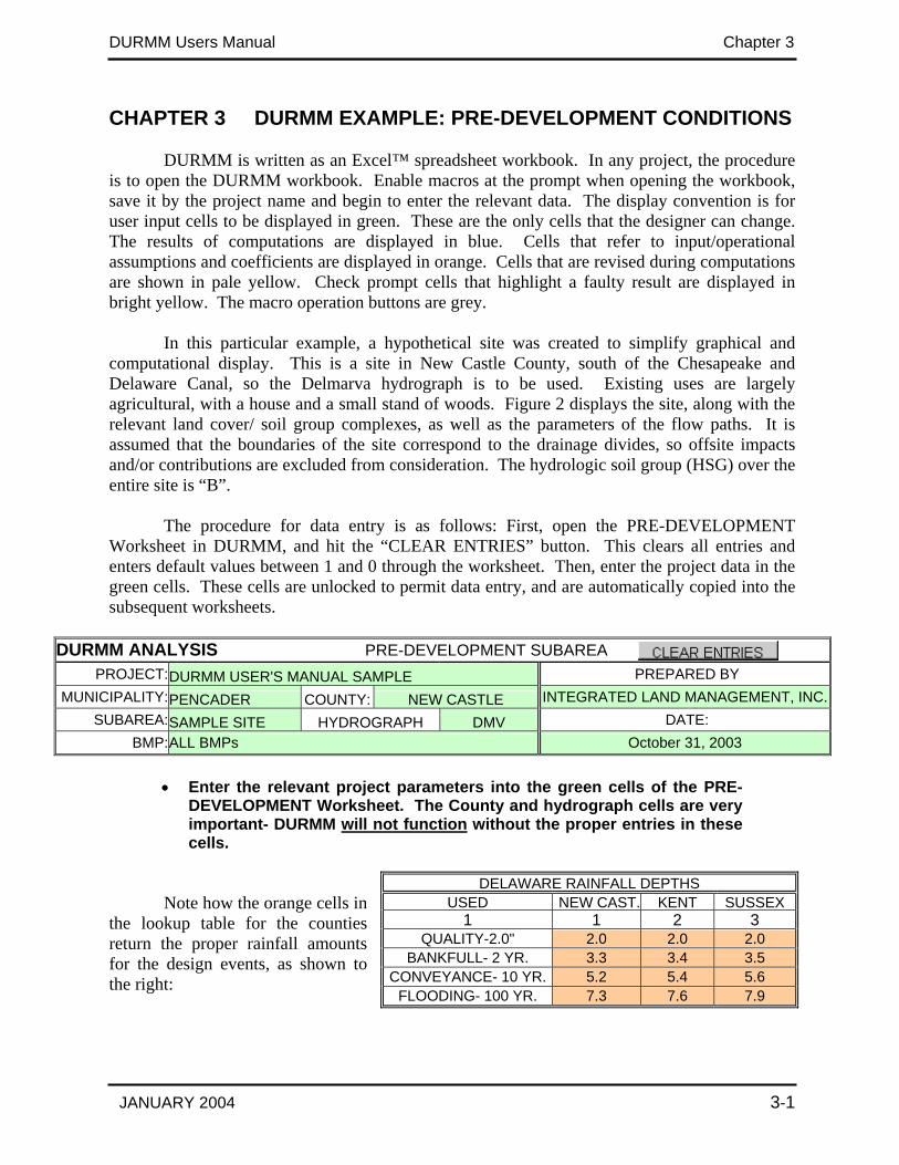
DURMM ANALYSIS PRE-DEVELOPMENT SUBAREA
PROJECT: DURMM USER'S MANUAL SAMPLE PREPARED BY MUNICIPALITY: PENCADER COUNTY: NEW CASTLE INTEGRATED LAND MANAGEMENT, INC.
SUBAREA: SAMPLE SITE HYDROGRAPH DMV DATE: BMP: ALL BMPs October 31, 2003
• Enter the relevant project parameters into the green cells of the PRE-
DEVELOPMENT Worksheet. The County and hydrograph cells are very important- DURMM will not function without the proper entries in these cells.
Note how the orange cells in
the lookup table for the counties return the proper rainfall amounts for the design events, as shown to the right:
DELAWARE RAINFALL DEPTHS USED NEW CAST. KENT SUSSEX
1 1 2 3QUALITY-2.0" 2.0 2.0 2.0
BANKFULL- 2 YR. 3.3 3.4 3.5 CONVEYANCE- 10 YR. 5.2 5.4 5.6
FLOODING- 100 YR. 7.3 7.6 7.9

DURMM Users Manual Chapter 3
JANUARY 2004 3-2
Figure 2: EXAMPLE SITE- Pre-development Conditions

DURMM Users Manual Chapter 3
JANUARY 2004 3-3
Next, enter the land cover/HSG complexes in the appropriate category cells. Since design software such as AutoCAD™ returns polygon areas in square feet, areas from the design can be entered directly. The HSG is also entered directly. Land cover type is entered by entering the proper code according to the look-up table shown below. Once the code is entered, the land cover name automatically is entered into the worksheet, the proper CN is entered into the area weighted CN routine, and the area is converted to acres. This table is displayed in the worksheet to simplify looking up the proper cover.
This procedure avoids errors from typographical mistakes. Any pervious entries over 12
or impervious entries less than 21 or greater than 26 will result in an “INVALID!” surface prompt, and enter an impossibly high CN value. Such entries will have to be corrected for the macros to run. This table is displayed in the worksheet next to the entry cells to facilitate looking up the proper cover. Note that impervious surfaces have the same CN, regardless of underlying soil, as would be expected. However, the CN values vary, instead of the uniform value of 98.0 used in TR-20.
SURFACE A B C D
1 WOODS-GD 30 55 70 77 2 WOODS-FR 36 60 73 79 3 MEADOW 30 58 71 78 4 PASTURE-GD 39 61 74 80 5 PASTURE-FR 49 69 79 84 6 CROPS-NT 61 70 77 80 7 CROPS-MT 64 75 82 85 8 CROPS-CT 67 78 85 89 9 LANDSCAPE-GD 36 60 73 77 10 LANDSCAPE-FR 49 69 79 84 11 LAWNS-GD 39 61 74 80 12 LAWNS-FR 49 69 79 84 21 PARKING LOT 99.7 22 SLOPE ROOF 99.7 23 FLAT ROOF 98.0 24 RES.STREET 97.1 25 RES.DRIVES 96.0 26 SIDEWALKS 96.0
The GD suffix represents good conditions, while the FR suffix represents fair conditions.
Crops are allocated as conventional tillage (CT), minimal till (MT) or no till plus cover crop (NT). Landscape is equivalent to Woods-FR in terms of CN, but it has higher phosphorus loading rates, hence its own category. Landscape-FR is applied to landscaping located in compacted areas around buildings. Lawns-FR is applied to ball fields and other high intensity park areas.
The criteria for pre-development conditions assume existing land cover. Regardless of
actual practices, agricultural crops should be classified as Crops–NT, as if they were crops using the best possible management practices. No-till (NT) crops are thus entered in the natural pervious category, along with pastures, meadows and woodlands, and all other codes up to 6. Minimum till (MT) and conventional till (CT) crops, landscaping and lawn codes from 7 to 12
DURMM Users Manual Chapter 3
JANUARY 2004 3-4
are classified as graded pervious, due to their extensive management inputs and proximity to structures. These cover classifications should not be entered into the natural pervious category.
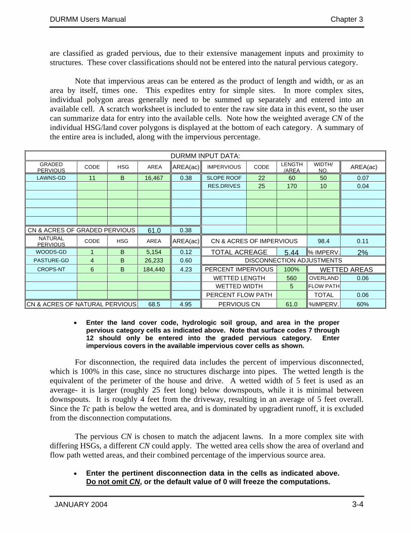
Note that impervious areas can be entered as the product of length and width, or as an
area by itself, times one. This expedites entry for simple sites. In more complex sites, individual polygon areas generally need to be summed up separately and entered into an available cell. A scratch worksheet is included to enter the raw site data in this event, so the user can summarize data for entry into the available cells. Note how the weighted average CN of the individual HSG/land cover polygons is displayed at the bottom of each category. A summary of the entire area is included, along with the impervious percentage.
DURMM INPUT DATA:
GRADED PERVIOUS CODE HSG AREA AREA(ac) IMPERVIOUS CODE LENGTH
/AREA WIDTH/
NO. AREA(ac)
LAWNS-GD 11 B 16,467 0.38 SLOPE ROOF 22 60 50 0.07 RES.DRIVES 25 170 10 0.04
CN & ACRES OF GRADED PERVIOUS 61.0 0.38 NATURAL PERVIOUS CODE HSG AREA AREA(ac) CN & ACRES OF IMPERVIOUS 98.4 0.11
WOODS-GD 1 B 5,154 0.12 TOTAL ACREAGE 5.44 % IMPERV. 2%PASTURE-GD 4 B 26,233 0.60 DISCONNECTION ADJUSTMENTS
CROPS-NT 6 B 184,440 4.23 PERCENT IMPERVIOUS 100% WETTED AREAS WETTED LENGTH 560 OVERLAND 0.06 WETTED WIDTH 5 FLOW PATH PERCENT FLOW PATH TOTAL 0.06
CN & ACRES OF NATURAL PERVIOUS 68.5 4.95 PERVIOUS CN 61.0 %IMPERV. 60% • Enter the land cover code, hydrologic soil group, and area in the proper
pervious category cells as indicated above. Note that surface codes 7 through 12 should only be entered into the graded pervious category. Enter impervious covers in the available impervious cover cells as shown.
For disconnection, the required data includes the percent of impervious disconnected,
which is 100% in this case, since no structures discharge into pipes. The wetted length is the equivalent of the perimeter of the house and drive. A wetted width of 5 feet is used as an average- it is larger (roughly 25 feet long) below downspouts, while it is minimal between downspouts. It is roughly 4 feet from the driveway, resulting in an average of 5 feet overall. Since the Tc path is below the wetted area, and is dominated by upgradient runoff, it is excluded from the disconnection computations.
The pervious CN is chosen to match the adjacent lawns. In a more complex site with
differing HSGs, a different CN could apply. The wetted area cells show the area of overland and flow path wetted areas, and their combined percentage of the impervious source area.
• Enter the pertinent disconnection data in the cells as indicated above. Do not omit CN, or the default value of 0 will freeze the computations.
DURMM Users Manual Chapter 3
JANUARY 2004 3-5
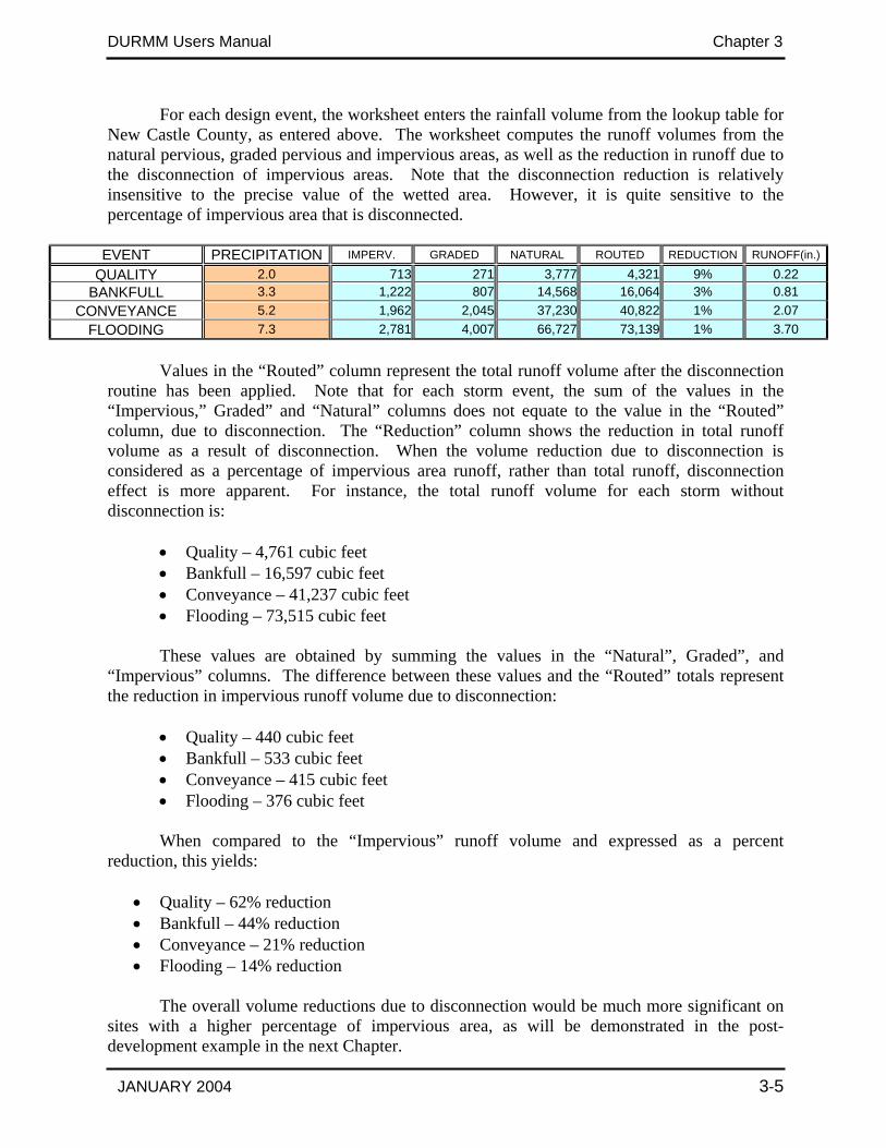
For each design event, the worksheet enters the rainfall volume from the lookup table for New Castle County, as entered above. The worksheet computes the runoff volumes from the natural pervious, graded pervious and impervious areas, as well as the reduction in runoff due to the disconnection of impervious areas. Note that the disconnection reduction is relatively insensitive to the precise value of the wetted area. However, it is quite sensitive to the percentage of impervious area that is disconnected.
EVENT PRECIPITATION IMPERV. GRADED NATURAL ROUTED REDUCTION RUNOFF(in.)
QUALITY 2.0 713 271 3,777 4,321 9% 0.22 BANKFULL 3.3 1,222 807 14,568 16,064 3% 0.81
CONVEYANCE 5.2 1,962 2,045 37,230 40,822 1% 2.07 FLOODING 7.3 2,781 4,007 66,727 73,139 1% 3.70
Values in the “Routed” column represent the total runoff volume after the disconnection
routine has been applied. Note that for each storm event, the sum of the values in the “Impervious,” Graded” and “Natural” columns does not equate to the value in the “Routed” column, due to disconnection. The “Reduction” column shows the reduction in total runoff volume as a result of disconnection. When the volume reduction due to disconnection is considered as a percentage of impervious area runoff, rather than total runoff, disconnection effect is more apparent. For instance, the total runoff volume for each storm without disconnection is:
• Quality – 4,761 cubic feet • Bankfull – 16,597 cubic feet • Conveyance – 41,237 cubic feet • Flooding – 73,515 cubic feet
These values are obtained by summing the values in the “Natural”, Graded”, and “Impervious” columns. The difference between these values and the “Routed” totals represent the reduction in impervious runoff volume due to disconnection:
• Quality – 440 cubic feet • Bankfull – 533 cubic feet • Conveyance – 415 cubic feet • Flooding – 376 cubic feet
When compared to the “Impervious” runoff volume and expressed as a percent reduction, this yields:
• Quality – 62% reduction • Bankfull – 44% reduction • Conveyance – 21% reduction • Flooding – 14% reduction
The overall volume reductions due to disconnection would be much more significant on sites with a higher percentage of impervious area, as will be demonstrated in the post-development example in the next Chapter.
DURMM Users Manual Chapter 3
JANUARY 2004 3-6
Once the subarea data is entered, the Tc path information is entered in the next series of
entry cells, according to the data set forth in the plans. The sheet flow parameters are typical to TR-20; a Manning’s n value of 0.45 is allocated to woods and 0.17 is allocated to crops.
Shallow flow parameters require more judgment. It is important to enter the correct
percentage of the entire disconnected area contributing to each swale, because DURMM computes its flow velocity based on this entry. Side slopes and bottom width are estimated from the plans; since shallow flow is by definition not confined to a channel. Instead, swales tend to have a wide bottoms and flat slopes which become more defined as they proceed downslope. For the upper segment in crops, a surface code 3 for short grass is applied, changing to a code of 4 for dense grass as it passes through the pasture. The upper segment receives 25 percent of the total runoff, while the lower segment receives all of the runoff.
SHEET FLOW PARAMETERS SWALE FLOW PARAMETERS FLOW PATHS LENGTH SLOPE Manning's n SURFACE FLOW % LENGTH SLOPE SIDES BOTTOM
UPPER 70 0.012 0.45 3 25% 295 0.014 10.0 4.0 LOWER 25 0.015 0.17 4 100% 385 0.017 8.0 2.0
• Enter sheet flow and shallow flow parameters per plan. Ensure that Manning’s
n values and surface codes accurately reflect land cover.
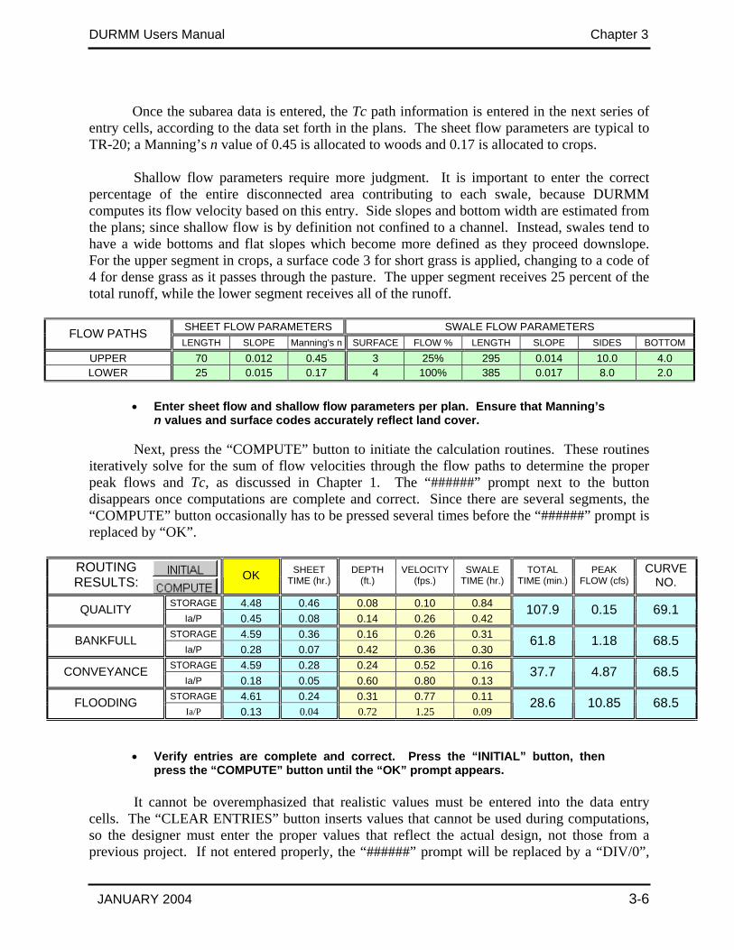
Next, press the “COMPUTE” button to initiate the calculation routines. These routines iteratively solve for the sum of flow velocities through the flow paths to determine the proper peak flows and Tc, as discussed in Chapter 1. The “######” prompt next to the button disappears once computations are complete and correct. Since there are several segments, the “COMPUTE” button occasionally has to be pressed several times before the “######” prompt is replaced by “OK”.
ROUTING
RESULTS: OK SHEET
TIME (hr.) DEPTH
(ft.) VELOCITY
(fps.) SWALE
TIME (hr.) TOTAL
TIME (min.) PEAK
FLOW (cfs)CURVE
NO.
STORAGE 4.48 0.46 0.08 0.10 0.84 QUALITY Ia/P 0.45 0.08 0.14 0.26 0.42
107.9 0.15 69.1
STORAGE 4.59 0.36 0.16 0.26 0.31 BANKFULL Ia/P 0.28 0.07 0.42 0.36 0.30
61.8 1.18 68.5
STORAGE 4.59 0.28 0.24 0.52 0.16 CONVEYANCE Ia/P 0.18 0.05 0.60 0.80 0.13
37.7 4.87 68.5
STORAGE 4.61 0.24 0.31 0.77 0.11 FLOODING Ia/P 0.13 0.04 0.72 1.25 0.09
28.6 10.85 68.5
• Verify entries are complete and correct. Press the “INITIAL” button, then press the “COMPUTE” button until the “OK” prompt appears.
It cannot be overemphasized that realistic values must be entered into the data entry
cells. The “CLEAR ENTRIES” button inserts values that cannot be used during computations, so the designer must enter the proper values that reflect the actual design, not those from a previous project. If not entered properly, the “######” prompt will be replaced by a “DIV/0”,
DURMM Users Manual Chapter 3
JANUARY 2004 3-7
“N/A” or “#NUM” prompt. Pressing the “COMPUTE” button under these circumstances will cause the macro routines to lock up, so the Visual Basic Editor will pop up, requesting “END” or “DEBUG”. If this occurs, press “END” at the prompt, confirm proper entries have been made and press the “INITIAL” button to clear erroneous intermediate values.
Having computed the velocities in the swales, the total Tc and peak flow computations
are returned. Storage is also calculated, along with the curve number. Note how the Tc decreases as the events increase. Also, note how the swale flow can be a substantial portion of the total Tc time. The values of Tc and CN from these computations can be directly entered as subarea data into other routing software when more complex hydrograph routing is required.
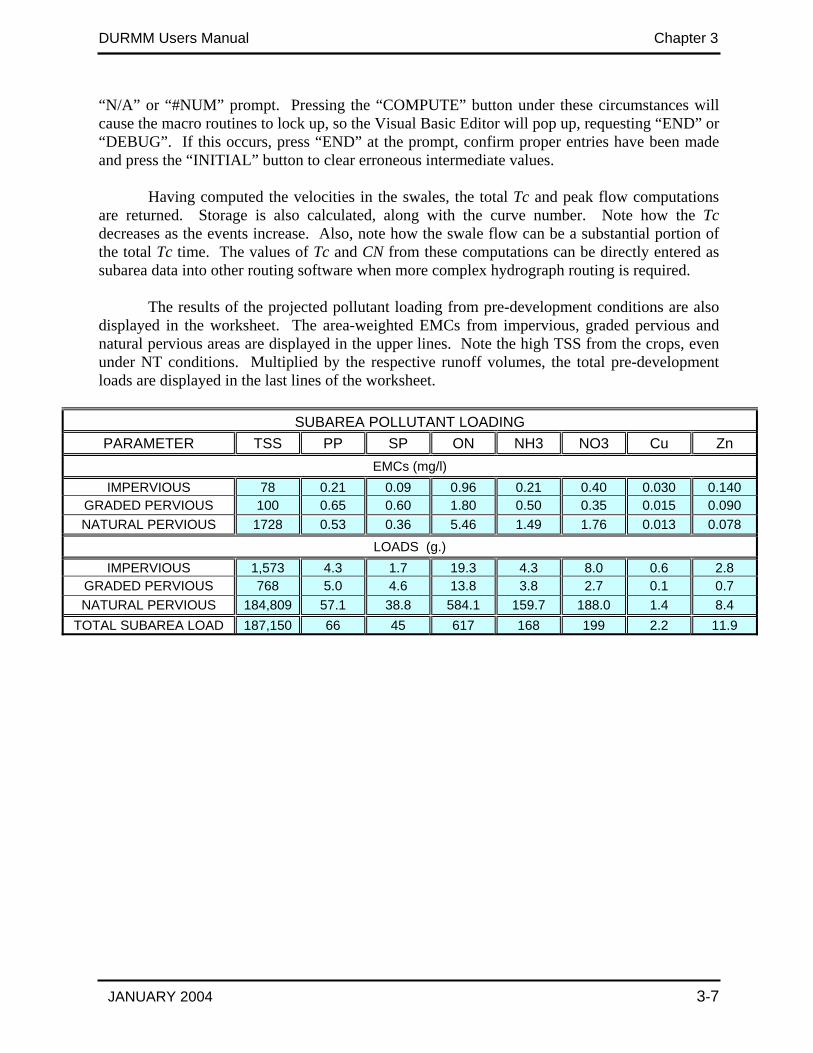
The results of the projected pollutant loading from pre-development conditions are also
displayed in the worksheet. The area-weighted EMCs from impervious, graded pervious and natural pervious areas are displayed in the upper lines. Note the high TSS from the crops, even under NT conditions. Multiplied by the respective runoff volumes, the total pre-development loads are displayed in the last lines of the worksheet.
SUBAREA POLLUTANT LOADING
PARAMETER TSS PP SP ON NH3 NO3 Cu Zn EMCs (mg/l)
IMPERVIOUS 78 0.21 0.09 0.96 0.21 0.40 0.030 0.140 GRADED PERVIOUS 100 0.65 0.60 1.80 0.50 0.35 0.015 0.090 NATURAL PERVIOUS 1728 0.53 0.36 5.46 1.49 1.76 0.013 0.078
LOADS (g.) IMPERVIOUS 1,573 4.3 1.7 19.3 4.3 8.0 0.6 2.8
GRADED PERVIOUS 768 5.0 4.6 13.8 3.8 2.7 0.1 0.7 NATURAL PERVIOUS 184,809 57.1 38.8 584.1 159.7 188.0 1.4 8.4
TOTAL SUBAREA LOAD 187,150 66 45 617 168 199 2.2 11.9
DURMM Users Manual Chapter 4
JANUARY 2004 4-1
CHAPTER 4 DURMM EXAMPLE: POST-DEVELOPMENT CONDITIONS
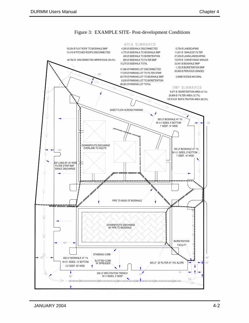
Figure 3 displays the post-development design of the Example Site. This is a mixed used office/commercial site with all of the BMPs; filter strips, conveyance and routing bioswales, a bioretention facility, and an infiltration trench. While it is unlikely that all of these BMPs would be incorporated into one BMP design workbook, they are included to demonstrate the potential of each BMP design. This example also illustrates many elements for integrating conservation design principles into overall site design.
Filter strips and conveyance bioswales are incorporated into the disconnected runoff
routines, reducing impervious runoff volumes prior to discharge into the bioswale. The lawns also reduce runoff from the rooftops in the disconnected areas before discharging into the bioswale, which fills an infiltration trench. This example illustrates some of the potential of DURMM’s capabilities, however, it should be noted that simpler designs without disconnection are possible where the site is not as complex. Elimination of the disconnection approach leads to a much shorter Tc into the BMPs.
It is important to note how the more distant impervious areas are disconnected. Runoff
from these surfaces is conveyed through two conveyance bioswales to the bioswale BMP, instead of discharging directly into the BMP. For this reason, the Tc path originates from these disconnected impervious surfaces. Pervious areas that are directly wetted by the adjacent impervious surfaces are allocated as disconnected, as well as pervious areas in the Tc path. Their contribution to total runoff is small compared to their effect on disconnection routines.
In the disconnected subarea, runoff from pitched roofs flows over the lawns between
buildings. Much of this lawn area is treated as wetted area from a filter strip, since roof downspouts are widely dispersed. Runoff from the parking lots flows into the upper bioswales, designed to provide as long a flow path as possible by being set at a 1% grade, and being wide enough to ensure submerged flow conditions. This results in long travel times through the swale, thus increasing Tc. This becomes particularly important at higher precipitation depths.
In the connected area, runoff from streets, sidewalks, roofs and driveways is directed into
the bioswale BMP. Along the bottom of the bioswale BMP, an infiltration trench BMP is proposed to further reduce runoff volumes and surface loading of pollutants. At the entrance where a convenience store would be located, the higher pollutant loads are to be treated by a bioretention facility.
Post-development allocation of areas and Tc pathways follows the procedures set forth in
the preceding section. Under post-development conditions, the pervious areas of the site in Figure 3 are distributed between natural pervious areas in woods, and pervious graded areas in lawn and landscaping. All soils are HSG B. The extent of disconnected and connected impervious area is broken down in detail, as is the extent of pervious areas receiving runoff from these impervious areas. This data is necessary to properly enter the appropriate values into the input and design worksheets. Refer to Figure 1 for a schematic of how DURMM routes runoff from the various source areas.
DURMM Users Manual Chapter 4
JANUARY 2004 4-2
Figure 3: EXAMPLE SITE- Post-development Conditions
DURMM Users Manual Chapter 4
JANUARY 2004 4-3
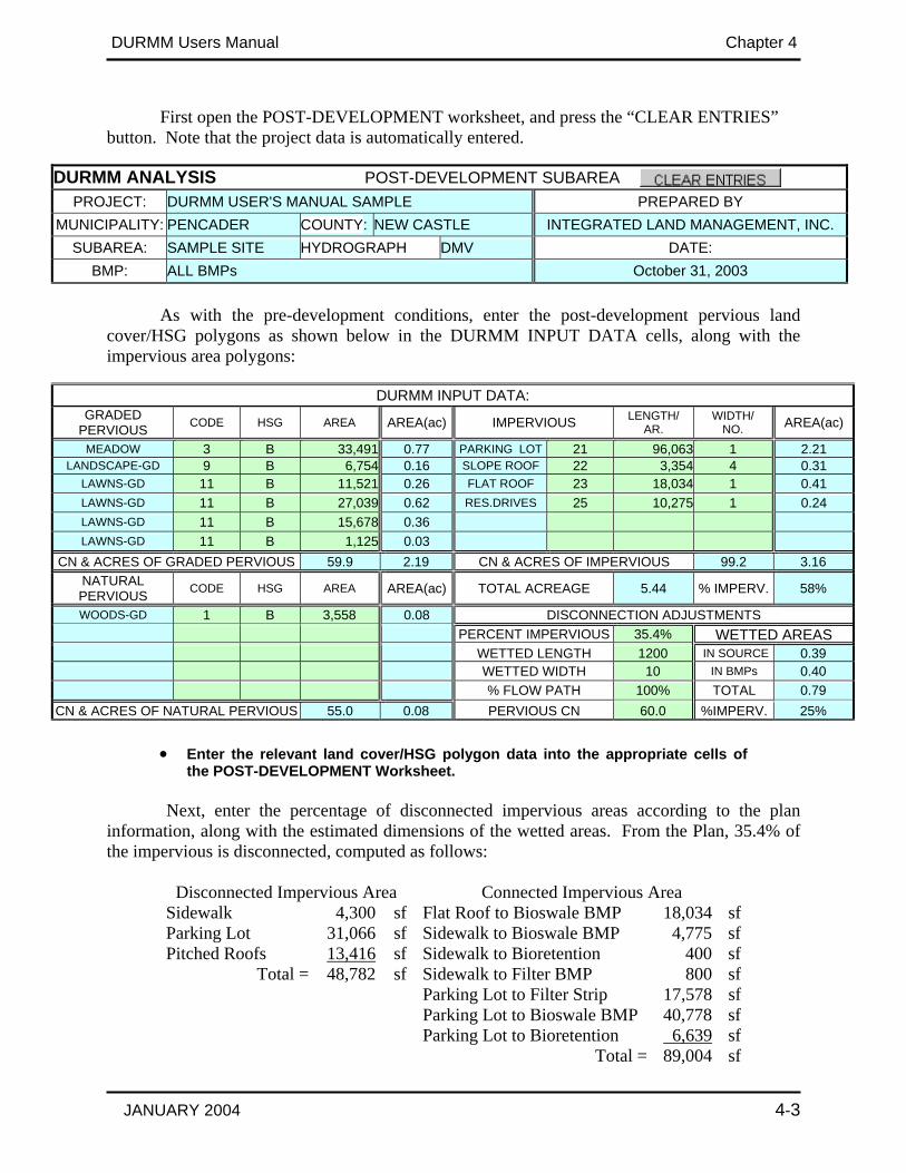
First open the POST-DEVELOPMENT worksheet, and press the “CLEAR ENTRIES” button. Note that the project data is automatically entered.
DURMM ANALYSIS POST-DEVELOPMENT SUBAREA PROJECT: DURMM USER'S MANUAL SAMPLE PREPARED BY
MUNICIPALITY: PENCADER COUNTY: NEW CASTLE INTEGRATED LAND MANAGEMENT, INC. SUBAREA: SAMPLE SITE HYDROGRAPH DMV DATE:
BMP: ALL BMPs October 31, 2003 As with the pre-development conditions, enter the post-development pervious land
cover/HSG polygons as shown below in the DURMM INPUT DATA cells, along with the impervious area polygons:
DURMM INPUT DATA:
GRADED PERVIOUS CODE HSG AREA AREA(ac) IMPERVIOUS LENGTH/
AR. WIDTH/
NO. AREA(ac)
MEADOW 3 B 33,491 0.77 PARKING LOT 21 96,063 1 2.21 LANDSCAPE-GD 9 B 6,754 0.16 SLOPE ROOF 22 3,354 4 0.31
LAWNS-GD 11 B 11,521 0.26 FLAT ROOF 23 18,034 1 0.41 LAWNS-GD 11 B 27,039 0.62 RES.DRIVES 25 10,275 1 0.24 LAWNS-GD 11 B 15,678 0.36 LAWNS-GD 11 B 1,125 0.03
CN & ACRES OF GRADED PERVIOUS 59.9 2.19 CN & ACRES OF IMPERVIOUS 99.2 3.16 NATURAL PERVIOUS CODE HSG AREA AREA(ac) TOTAL ACREAGE 5.44 % IMPERV. 58%
WOODS-GD 1 B 3,558 0.08 DISCONNECTION ADJUSTMENTS PERCENT IMPERVIOUS 35.4% WETTED AREAS WETTED LENGTH 1200 IN SOURCE 0.39 WETTED WIDTH 10 IN BMPs 0.40 % FLOW PATH 100% TOTAL 0.79
CN & ACRES OF NATURAL PERVIOUS 55.0 0.08 PERVIOUS CN 60.0 %IMPERV. 25%
• Enter the relevant land cover/HSG polygon data into the appropriate cells of the POST-DEVELOPMENT Worksheet.
Next, enter the percentage of disconnected impervious areas according to the plan
information, along with the estimated dimensions of the wetted areas. From the Plan, 35.4% of the impervious is disconnected, computed as follows:
Disconnected Impervious Area Connected Impervious Area
Sidewalk 4,300 sf Flat Roof to Bioswale BMP 18,034 sfParking Lot 31,066 sf Sidewalk to Bioswale BMP 4,775 sfPitched Roofs 13,416 sf Sidewalk to Bioretention 400 sf
Total = 48,782 sf Sidewalk to Filter BMP 800 sf Parking Lot to Filter Strip 17,578 sf Parking Lot to Bioswale BMP 40,778 sf Parking Lot to Bioretention 6,639 sf Total = 89,004 sf

DURMM Users Manual Chapter 4
JANUARY 2004 4-4
Total impervious area = 48,782 sf + 89,004 sf = 137,786 sf % disconnected impervious area = 48,782/137,786 = 35.4%
The wetted length is equal to the perimeter of the buildings, the width is 10 feet, and the
entire conveyance path is included in the wetted area. The wetted area curve number is 60, which represents the average CN of the pervious graded areas. The wetted area in the source area is 0.39 acres. The BMP wetted areas will be discussed below in the section on BMP design.
• Enter percentage of impervious areas disconnected per plan. Enter
disconnection length, width, percent of flow path, and curve number. Following cell entry, the runoff volume summary displays the volumes from each
category of land cover. Note the substantial reduction in runoff to the BMPs from the sum of runoff categories due to disconnection. The total volume reduction takes into account the disconnection losses in the BMPs, which includes the losses from the infiltration trench. These fields for BMP reductions are discussed at the section on BMP design at the end of this chapter, once their design has been addressed.
After the subarea data is entered, the Tc path information is entered in the next series of entry cells, according to the data set forth in the plans. For the Example Site, sheet flow originates from the parking lot for 60 feet at 1.0%, thence discharging into the upper bioswale. In this case, Manning’s n for the upper segment assumes pavement with a value of 0.011. No lower sheet flow segment is applicable. Shallow flow parameters are taken directly from the plans. The percent of area in the swale entry cells represents the contributing area of the total site to be allocated to each swale segment. Just as in pre-development conditions, it is important to enter the correct percentage of the entire area contributing to each swale. Since the bioswales are turf, surface code 4 for dense turf is applied. At a slope of 1%, these swales are designed to not only filter runoff, but also to reduce velocities and increase Tc.
SHEET FLOW PARAMETERS SWALE FLOW PARAMETERS
FLOW PATHS LENGTH SLOPE Manning's n SURFACE FLOW % LENGTH SLOPE SIDES BOTTOM
UPPER 70 0.0100 0.011 4 25% 380 0.010 4.0 6.0 LOWER 4 35% 180 0.010 4.0 16.0
% RUNOFF 94% Tc Path IMPERV 4 82% 600 0.010 8.0 12.0
• Enter sheet flow and shallow flow parameters per plan. Ensure that Manning’s
n values and surface codes accurately reflect land cover. The worksheet indicates that 94 percent of the runoff from the quality event originates
from impervious surfaces, resulting in the “IMPERV” prompt in the yellow cell for the Tc path.
EVENT PRECIP. NATURAL GRADED IMPERV. TO BMPs
QUALITY 2.0 6 1,403 21,971 19,199 BANKFULL 3.3 83 4,352 36,898 36,691
CONVEYANCE 5.2 320 11,234 58,560 66,630 FLOODING 7.3 688 22,388 82,673 102,652

DURMM Users Manual Chapter 4
JANUARY 2004 4-5
For this reason, the Tc path must originate from impervious surfaces. The swale entries in blue at the bottom reflect design parameters of the bioswale BMP design to be discussed below.
Following data entry, the SUBAREA POLLUTANT LOADING cells at the bottom
display the area-weighted EMCs and corresponding mass loads from the land cover categories. Note how loads are dominated by the impervious surfaces, even though their EMCs are relatively low. This is due to the much greater volume of runoff involved.
SUBAREA POLLUTANT LOADING PARAMETER TSS PP SP ON NH3 NO3 Cu Zn
IMPERVIOUS EMCs (mg/l) 59 0.19 0.06 1.14 0.43 0.34 0.030 0.140 GRADED PERVIOUS EMCs (mg/l) 75 0.69 0.55 1.78 0.46 0.31 0.010 0.057
NATURAL PERVIOUS EMCs (mg/l) 15 0.65 0.35 1.75 0.40 0.25 0.001 0.005 IMPERVIOUS LOADS (g.) 36,814 121.1 35.8 706.9 270.3 212.0 18.7 87.1
GRADED PERVIOUS LOADS (g.) 2,997 27.5 21.8 70.7 18.3 12.2 0.4 2.3 NATURAL PERVIOUS LOADS (g.) 3 0.1 0.1 0.3 0.1 0.0 0.0 0.0
TOTAL SUBAREA LOAD 39,814 149 58 778 289 224 19.1 89.4 Since the basis of DURMM is the integration of the BMPS into the design, it is necessary
to switch to the BMP DESIGN worksheet and design the BMPs to obtain the final routing results. Results from the design affect the runoff reduction volumes for the disconnected BMPs. Once these procedures are completed as discussed below, DURMM generates the preceding summary table of the resulting runoff volumes. Note that the total with BMPs is less than the sum of the unrouted runoff volumes, particularly for the smaller events. In this example, these reductions are substantial due to disconnection routines applied to the BMPs.
The procedure for BMP design is as follows: First open the “BMP DESIGN” worksheet, and press the “CLEAR ENTRIES” button.
DURMM ANALYSIS BMP DESIGN DATA & RESULTS
PROJECT: DURMM USER'S MANUAL SAMPLE PREPARED BY MUNICIPALITY: PENCADER COUNTY: NEW CASTLE INTEGRATED LAND MANAGEMENT, INC.
SUBAREA: SAMPLE SITE HYDROGRAPH DMV DATE: BMP: ALL BMPs October 31, 2003
PARAMETER TSS PP SP ON NH3 NO3 Cu Zn INPUT CONCENTRATION 60.1 0.22 0.09 1.17 0.44 0.34 0.029 0.135 INPUT MASS LOADS (g) 32,695 122 47 639 237 184 16 73
INCREASE IN SUBAREA LOAD (154,455) 56 2 21 69 (14) 13 61 % PREDEVELOPMENT LOAD 17% 184% 105% 103% 141% 93% 724% 617%
The input concentration represents the total load divided by total runoff volume from the
source categories. Note how the input mass loads to the BMPs are slightly less than the output loads displayed in the pre-development analysis. This is due to the reductions in runoff volumes due to disconnection in the source areas. The last two rows compare loads to pre-development conditions. Note how the pre-development conditions result in much more TSS loads than post-
DURMM Users Manual Chapter 4
JANUARY 2004 4-6
development conditions, while the metal loads under post-development conditions substantially increase.
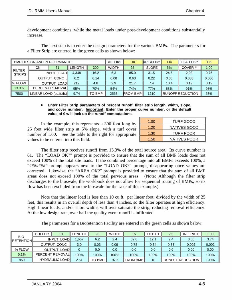
The next step is to enter the design parameters for the various BMPs. The parameters for
a Filter Strip are entered in the green cells as shown below:
BMP DESIGN AND PERFORMANCE BIO. OK? OK AREA OK? OK LOAD OK? OK CN 61 LENGTH 300 WIDTH 25 SLOPE 5% COVER # 1.00
INPUT LOAD 4,348 16.2 6.3 85.0 31.5 24.5 2.08 9.76 FILTER
STRIPS OUTPUT CONC . 6.2 0.14 0.08 0.63 0.22 0.30 0.005 0.006
% FLOW OUTPUT LOAD 212 4.8 2.9 21.7 7.4 10.4 0.19 0.19 13.3% PERCENT REMOVAL 95% 70% 54% 74% 77% 58% 91% 98% 7500 LINEAR LOAD (cu.ft./ft.) 9.74 TO BMP 2553 FROM BMP 1210 RUNOFF REDUCTION 53%
• Enter Filter Strip parameters of percent runoff, filter strip length, width, slope,
and cover number. Important: Enter the proper curve number, or the default value of 0 will lock up the runoff computations.
In the example, this represents a 300 foot long by
25 foot wide filter strip at 5% slope, with a turf cover number of 1.00. See the table to the right for appropriate values to be entered into this field.
The filter strip receives runoff from 13.3% of the total source area. Its curve number is
61. The “LOAD OK?” prompt is provided to ensure that the sum of all BMP loads does not exceed 100% of the total site loads. If the combined percentage into all BMPs exceeds 100%, a “#######” prompt appears next to the “LOAD OK?” prompt, disappearing once values are corrected. Likewise, the “AREA OK?” prompt is provided to ensure that the sum of all BMP areas does not exceed 100% of the total pervious areas. (Note: Although the filter strip discharges to the bioswale, the workbook does not allow for sequential routing of BMPs, so its flow has been excluded from the bioswale for the sake of this example.)
Note that the linear load is less than 10 cu.ft. per linear foot; divided by the width of 25
feet, this results in an overall depth of less than 4 inches, so the filter operates at high efficiency. High linear loads, and/or short widths will over-saturate the strip, reducing removal efficiency. At the low design rate, over half the quality event runoff is infiltrated.
The parameters for a Bioretention Facility are entered in the green cells as shown below:
BUFFER 10 LENGTH 25 WIDTH 15 DEPTH 2.5 INF. RATE 1.00 INPUT LOAD 1,667 6.2 2.4 32.6 12.1 9.4 0.80 3.74
BIO- RETENTION
OUTPUT CONC . 3.0 0.03 0.09 0.78 0.34 0.33 0.002 0.002 % FLOW OUTPUT LOAD 0 0.0 0.0 0.0 0.0 0.0 0.00 0.00
5.1% PERCENT REMOVAL 100% 100% 100% 100% 100% 100% 100% 100% 850 HYDRAULIC LOAD 2.61 TO BMP 979 FROM BMP 0 RUNOFF REDUCTION 100%
1.00 TURF GOOD 1.20 NATIVES GOOD 1.30 TURF POOR 1.50 NATIVES POOR

DURMM Users Manual Chapter 4
JANUARY 2004 4-7
• Enter Bioretention parameters of percent runoff, buffer width, and bioretention media length, width, depth and infiltration rate.
Entries display a 15 foot wide by 25 foot long bioretention facility, with buffer width of
10 feet surrounding the media. It receives runoff from 5.1% of the total site area, and the buffer area outside the bioretention media has a curve number of 61. The 850 in the area cell provides the wetted area data for DURMM to compute the additional infiltration as sheet flow enters the sides of the facility. The “BIO OK?” prompt is provided to ensure the bioretention media is not overloaded at a hydraulic loading rate above 2.75 feet over the bioretention media area. When loading is too high, a “#######” prompt appears, disappearing once appropriate dimensions are entered.
The parameters for a Biofiltration Swale are entered in the green cells as shown below:
CN 55 LENGTH 600 SIDES:1 6.0 BOTTOM 12.0 SWALE OK? OK SLOPE 1.0% COVER 4 DENSE GRASS VELOCITY 0.22 DEPTH 0.12
INPUT LOAD 26,679 100 39 521 193 150 12.77 59.88
BIOSWALE QUALITY DESIGN
OUTPUT CONC . 4.1 0.10 0.08 0.62 0.26 0.30 0.005 0.013 % FLOW OUTPUT LOAD 1,287 30.8 24.9 193.2 81.0 92.4 1.53 3.98
81.6% PERCENT REMOVAL 95% 69% 35% 63% 58% 39% 88% 93% 9000 RESIDENCE TIME (min.) 46.0 TO BMP 15667 FROM BMP 10972 RUNOFF REDUCTION 30%
• Enter Biofiltration Swale parameters of percent impervious source area, length,
side slopes, width, slope, and surface code. Important: Enter the proper curve number, or the default value of 0 will lock up the runoff computations.
Entries display a 12 foot wide by 600 foot long bioswale, with side slopes of 6:1, and a
slope of 1%. It receives the runoff from the balance of total site area, or 81.6% (100% - 13.3% - 5.1%). Representing a meadow cover, the surface code of 4 generates the “DENSE GRASS” prompt, and gives a CN of 55 to be entered. Check the “LOAD OK?” prompt discussed for filter strips to ensure that sum of entries does not exceed 100%. Upon pressing the “SWALE” button, the bioswale routines then compute the velocity, depth and residence time. When correctly computed, the “#######” prompt next the SWALE OK? cell is replaced by the “OK” prompt.
Note: the results of this computation step are affected by subsequent infiltration trench
design entries and how they affect runoff volumes and subsequent peak flow computations. The values entered represent the final stabilized values after these procedures are completed. Therefore, the swale button may have to be pressed again to obtain the final proper result after designing the infiltration trench as below.
From these hydraulic parameters, DURMM computes the reduction in EMCs in the
bioswales. Note how its meadow cover, wide width, shallow side slopes, long length, and shallow slope serve to create a residence time of 46.0 minutes. This is due to the shallow depth of flow of less than 2 inches and a flow velocity of 0.22 fps. Since its hydraulic loading rate is higher than the filter strips, there is less percentage of runoff reduction than the filter strip for the quality event. However, there is a substantial reduction in runoff volume due to its large size.
DURMM Users Manual Chapter 4
JANUARY 2004 4-8
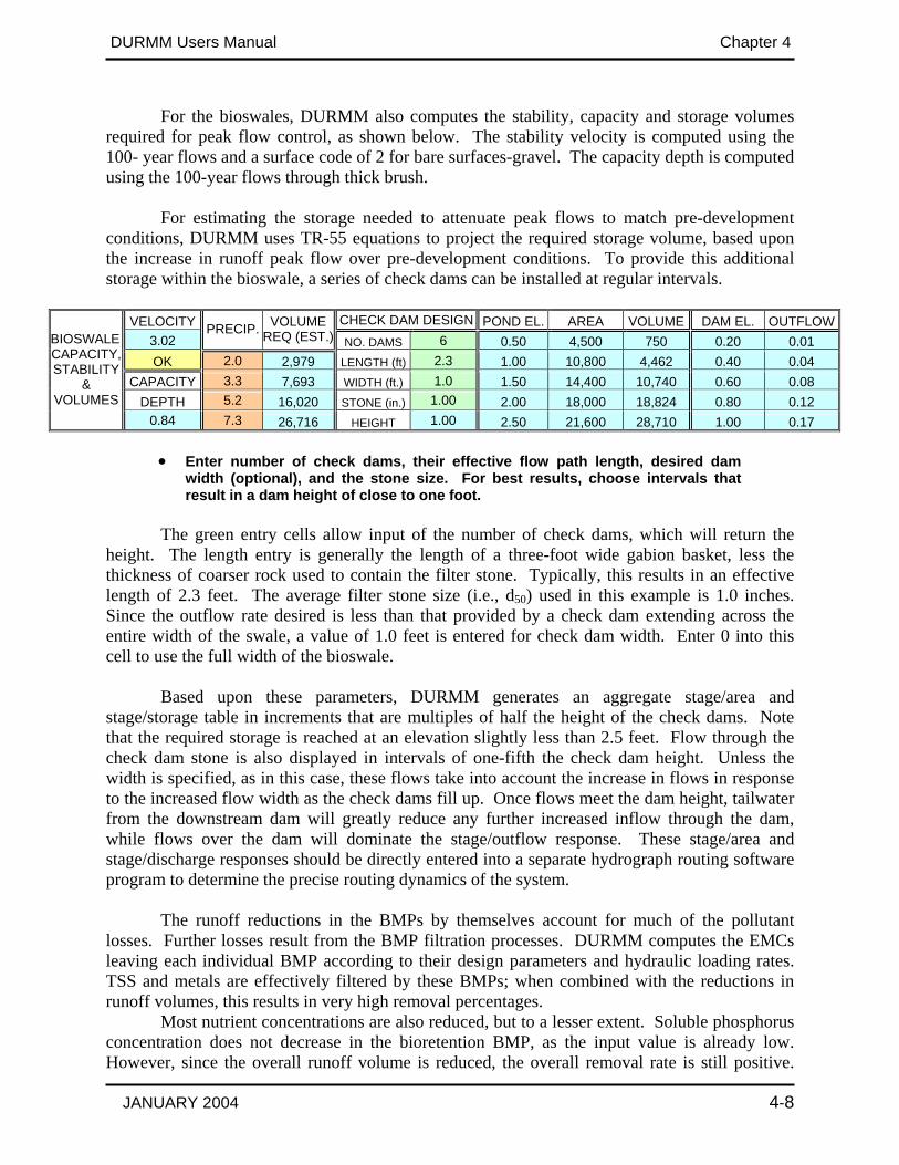
For the bioswales, DURMM also computes the stability, capacity and storage volumes required for peak flow control, as shown below. The stability velocity is computed using the 100- year flows and a surface code of 2 for bare surfaces-gravel. The capacity depth is computed using the 100-year flows through thick brush.
For estimating the storage needed to attenuate peak flows to match pre-development
conditions, DURMM uses TR-55 equations to project the required storage volume, based upon the increase in runoff peak flow over pre-development conditions. To provide this additional storage within the bioswale, a series of check dams can be installed at regular intervals.
VELOCITY CHECK DAM DESIGN POND EL. AREA VOLUME DAM EL. OUTFLOW
3.02 PRECIP. VOLUME
REQ (EST.) NO. DAMS 6 0.50 4,500 750 0.20 0.01 OK 2.0 2,979 LENGTH (ft) 2.3 1.00 10,800 4,462 0.40 0.04
CAPACITY 3.3 7,693 WIDTH (ft.) 1.0 1.50 14,400 10,740 0.60 0.08 DEPTH 5.2 16,020 STONE (in.) 1.00 2.00 18,000 18,824 0.80 0.12
BIOSWALE CAPACITY, STABILITY
& VOLUMES
0.84 7.3 26,716 HEIGHT 1.00 2.50 21,600 28,710 1.00 0.17 • Enter number of check dams, their effective flow path length, desired dam
width (optional), and the stone size. For best results, choose intervals that result in a dam height of close to one foot.
The green entry cells allow input of the number of check dams, which will return the
height. The length entry is generally the length of a three-foot wide gabion basket, less the thickness of coarser rock used to contain the filter stone. Typically, this results in an effective length of 2.3 feet. The average filter stone size (i.e., d50) used in this example is 1.0 inches. Since the outflow rate desired is less than that provided by a check dam extending across the entire width of the swale, a value of 1.0 feet is entered for check dam width. Enter 0 into this cell to use the full width of the bioswale.
Based upon these parameters, DURMM generates an aggregate stage/area and
stage/storage table in increments that are multiples of half the height of the check dams. Note that the required storage is reached at an elevation slightly less than 2.5 feet. Flow through the check dam stone is also displayed in intervals of one-fifth the check dam height. Unless the width is specified, as in this case, these flows take into account the increase in flows in response to the increased flow width as the check dams fill up. Once flows meet the dam height, tailwater from the downstream dam will greatly reduce any further increased inflow through the dam, while flows over the dam will dominate the stage/outflow response. These stage/area and stage/discharge responses should be directly entered into a separate hydrograph routing software program to determine the precise routing dynamics of the system.
The runoff reductions in the BMPs by themselves account for much of the pollutant
losses. Further losses result from the BMP filtration processes. DURMM computes the EMCs leaving each individual BMP according to their design parameters and hydraulic loading rates. TSS and metals are effectively filtered by these BMPs; when combined with the reductions in runoff volumes, this results in very high removal percentages.
Most nutrient concentrations are also reduced, but to a lesser extent. Soluble phosphorus concentration does not decrease in the bioretention BMP, as the input value is already low. However, since the overall runoff volume is reduced, the overall removal rate is still positive.

DURMM Users Manual Chapter 4
JANUARY 2004 4-9
These results emphasize the importance of the runoff reduction aspect of Green Technology BMPs.
SUMMARY OF FILTERING BMP PERFORMANCE
PARAMETER TSS PP SP ON NH3 NO3 Cu Zn STRIP & SWALE OUTPUT LOAD
( )1,498 35.6 27.8 215.0 88.4 102.7 1.72 4.17
ALL BMPs OUTPUT LOAD (g) 1,498 35.6 27.8 215.0 88.4 102.7 1.72 4.17 PERCENT REMOVAL 95% 71% 41% 66% 63% 44% 89% 94%
Mass loads from the filter strip and bioswale BMPs are summed and divided by the
resultant runoff volumes to develop the average EMCs and mass loads leaving these surface BMPs. “All BMPs Output Load” includes the load from the bioretention facility. Filter strip and bioswale output loads are segregated from the bioretention loads so they can be directed to an infiltration trench BMP for further volume losses. Bioretention loads are infiltrated separately in a manner similar to the infiltration trench BMP routines, as discussed below. In this example, the percentage of mass loads removed varies from 41% to 95%.
To provide for further reduction in surface runoff loads and increase site recharge, an
infiltration trench BMP is included. In this particular case, all of the surface runoff is directed to a 300 foot long by 3 foot wide trench 3 feet deep, with an infiltration rate of 2.0 inches per hour.
The resulting entry cells for this option are indicated below:
% SURFACE 100.0% LENGTH: 300 WIDTH: 3.0 DEPTH: 3 INF. RATE 2.00
INFILTRATED LOAD 569 13.5 10.6 81.6 33.6 39.0 0.65 1.58 INFILT-
RATION. TRENCH
INFILTRATION TIME 23.6 TO BMP 12182 FROM BMP 7557 RUNOFF REDUCTION 38%
• Enter per cent of surface runoff, trench length, width, depth and infiltration
rates.
The void ratio of the stone media is allocated at 40 per cent. The infiltration area of the bottom is multiplied by the infiltration rate over a period of 24 hours (the duration of the storm event) to obtain the infiltration during the storm. Runoff reductions are based upon infiltration through the bottom over this 24-hour period, plus the volume stored in the trench. Under these circumstances, the trench reduces the runoff volume by 38 per cent. No reductions in EMCs are allocated to infiltration trenches; instead, the runoff volume is treated as if it were lost from the system.
After passing through this treatment train, the combined mass loads leaving the BMPs
are summarized in the final cells. Compared to the loads leaving the individual land cover categories, the percent removal varies from 64% to 97%, depending upon the pollutant. Excluding TSS (which is nearly eliminated when compared to crops) mass loads leaving the site are at most 22% of the pre-development loads.
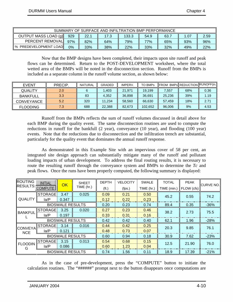
DURMM Users Manual Chapter 4
JANUARY 2004 4-10
SUMMARY OF SURFACE AND INFILTRATION BMP PERFORMANCE OUTPUT MASS LOAD (g) 929 22.1 17.3 133.3 54.9 63.7 1.07 2.59
PERCENT REMOVAL 97% 82% 64% 79% 77% 65% 93% 96% % PREDEVELOPMENT LOAD 0% 33% 38% 22% 33% 32% 49% 22%
Now that the BMP designs have been completed, their impacts upon site runoff and peak
flows can be determined. Return to the POST-DEVELOPMENT worksheet, where the total wetted area of the BMPs will be noted in the disconnection section. Runoff from the BMPs is included as a separate column in the runoff volume section, as shown below:
EVENT PRECIP. NATURAL GRADED IMPERV. TO BMPs FROM BMPs REDUCTION RUNOFF(in.
)QUALITY 2.0 6 1,403 21,971 19,199 7,557 68% 0.36
BANKFULL 3.3 83 4,352 36,898 36,691 25,236 39% 1.19 CONVEYANCE 5.2 320 11,234 58,560 66,630 57,459 18% 2.71
FLOODING 7.3 688 22,388 82,673 102,652 96,006 9% 4.53
Runoff from the BMPs reflects the sum of runoff volumes discussed in detail above for
each BMP during the quality event. The same disconnection routines are used to compute the reductions in runoff for the bankfull (2 year), conveyance (10 year), and flooding (100 year) events. Note that the reductions due to disconnection and the infiltration trench are substantial, particularly for the quality event that dominates the annual runoff response.
As demonstrated in this Example Site with an impervious cover of 58 per cent, an
integrated site design approach can substantially mitigate many of the runoff and pollutant loading impacts of urban development. To address the final routing results, it is necessary to route the resulting runoff through the conveyance system and BMPs to determine the Tc and peak flows. Once the runs have been properly computed, the following summary is displayed:
DEPTH VELOCITY SWALE TOTAL PEAK ROUTING
RESULTS: OK SHEET TIME (hr.) (ft.) (fps.) TIME (hr.) TIME (min.) FLOW (cfs)
CURVE NO.
STORAGE 3.47 0.025 0.09 0.21 0.50 Ia/P 0.347 0.12 0.22 0.23
45.2 0.55 74.2 QUALITY
BIOSWALE RESULTS 0.20 0.23 0.74 89.4 0.35 -36% STORAGE 3.25 0.020 0.27 0.23 0.46
Ia/P 0.197 0.33 0.31 0.16 38.2 2.73 75.5 BANKFUL
L BIOSWALE RESULTS 0.42 0.42 0.40 62.1 1.96 -28%
STORAGE 3.14 0.016 0.44 0.42 0.25 Ia/P 0.121 0.48 0.73 0.07
20.3 9.85 76.1 CONVEYANCE
BIOSWALE RESULTS 0.60 0.94 0.18 30.9 7.62 -23% STORAGE 3.15 0.013 0.54 0.68 0.15
Ia/P 0.086 0.60 1.23 0.04 12.5 21.90 76.0 FLOODIN
G BIOSWALE RESULTS 0.74 1.56 0.11 18.9 17.39 -21%
As in the case of pre-development, press the “COMPUTE” button to initiate the
calculation routines. The “######” prompt next to the button disappears once computations are
DURMM Users Manual Chapter 4
JANUARY 2004 4-11
complete and correct. Since there are several segments, the “COMPUTE” button occasionally has to be pressed several times before the “######” prompt is replaced by “OK”.
Again, it cannot be overemphasized that realistic values must be entered into data entry
cells. If the Visual Basic Editor pops up, requesting “END” or “DEBUG”, press the “END” prompt, confirm proper entries have been made and press the “INITIAL” button to clear erroneous interim values.
Note that the sheet flow paths are very short, reflecting the impervious source area.
However, the effect of designing a circuitous bioswale conveyance system results in a Tc that is still quite long for the quality event. As in the case of pre-development, the Tc length decreases as event size increases. Storage is calculated from precipitation and runoff volumes; given storage, the curve number is computed. Due to the infiltration trench reducing effective CN so much in the smaller events, the effective CN actually increases as the event size increases.
Given the Tc and Ia/P, TR-55 routines are then used to compute the peak flow into the
BMPs. This is shown as the top line for each event. To determine the effect of the bioswale BMP in further delaying the Tc, its travel time for each event is displayed in the third line of blue cells for each event. The resulting Tc is then displayed, along with the resulting peak flow, and the reduction in peak as a percentage. Note how the additional travel times in the bioswale decrease peak flows by 21 to 36 percent, depending upon the event size.
In order to route these flows through the bioswale or another detention BMP, and/or
combine hydrographs from several different subareas, it is necessary to enter the preceding results into a separate routing software package. Since Tc and CN vary from event to event, it is necessary to enter the pre- and post-development subarea data for each event, using the direct entry option to enter these parameters, along with subarea size.
For routing bioswales with check dams, the stage/area and stage/discharge relationships
discussed above are similarly entered into a separate routing software package. If the outlet structure from the bioswale is a different type of structure than the check dams, the last pool should be modeled as a separate pond, with the stage/area summaries allocated between the pools proportionately. In situations where the most accurate results are required, it is necessary to route each pond individually, using dynamic routing software that takes into account the tailwater effects between the pools at each time step.
The preceding analysis shows that, by designing the stormwater collection, conveyance
and filtration BMPs to increase Tc, substantial reductions in peak flows occur. While the resulting peak flows are still higher than pre-development conditions, they are substantially less than twice as high, even on site with nearly 60 per cent impervious cover. This example demonstrates the benefits of an integrated Green Technology approach to site layout and BMP design.

DURMM Users Manual Chapter 4
JANUARY 2004 4-12
This page left intentionally blank.

DURMM Users Manual Appendix A – Users Guide
JANUARY 2004
Appendix A
Users Guide

DURMM Users Manual Appendix A – Users Guide
JANUARY 2004
This page left intentionally blank.
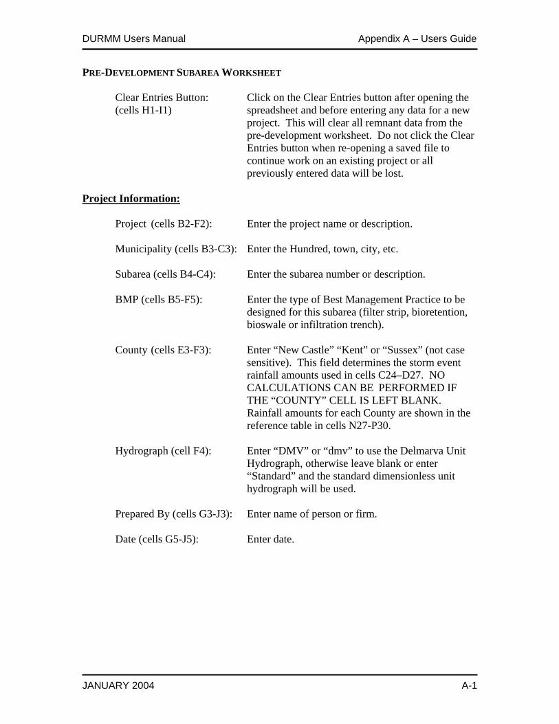
DURMM Users Manual Appendix A – Users Guide
JANUARY 2004 A-1
PRE-DEVELOPMENT SUBAREA WORKSHEET Clear Entries Button: Click on the Clear Entries button after opening the (cells H1-I1) spreadsheet and before entering any data for a new project. This will clear all remnant data from the pre-development worksheet. Do not click the Clear Entries button when re-opening a saved file to continue work on an existing project or all previously entered data will be lost. Project Information:
Project (cells B2-F2): Enter the project name or description. Municipality (cells B3-C3): Enter the Hundred, town, city, etc. Subarea (cells B4-C4): Enter the subarea number or description. BMP (cells B5-F5): Enter the type of Best Management Practice to be designed for this subarea (filter strip, bioretention, bioswale or infiltration trench). County (cells E3-F3): Enter “New Castle” “Kent” or “Sussex” (not case sensitive). This field determines the storm event rainfall amounts used in cells C24–D27. NO CALCULATIONS CAN BE PERFORMED IF THE “COUNTY” CELL IS LEFT BLANK. Rainfall amounts for each County are shown in the reference table in cells N27-P30. Hydrograph (cell F4): Enter “DMV” or “dmv” to use the Delmarva Unit Hydrograph, otherwise leave blank or enter “Standard” and the standard dimensionless unit hydrograph will be used. Prepared By (cells G3-J3): Enter name of person or firm. Date (cells G5-J5): Enter date.
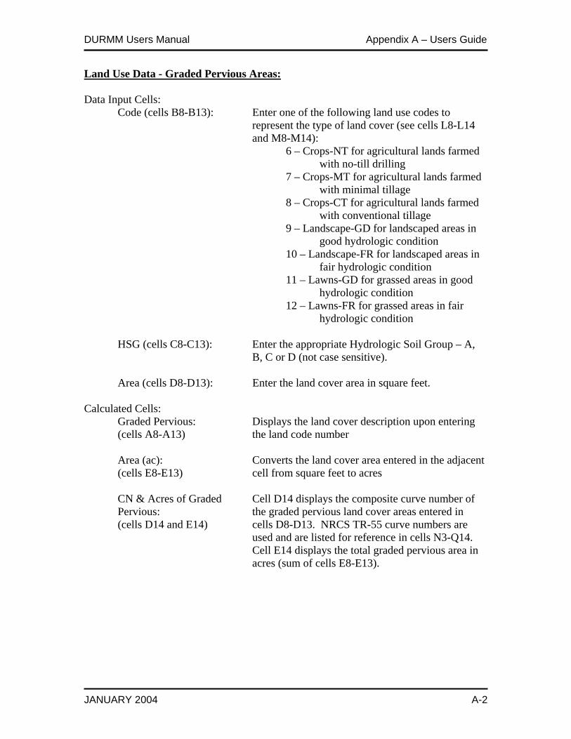
DURMM Users Manual Appendix A – Users Guide
JANUARY 2004 A-2
Land Use Data - Graded Pervious Areas: Data Input Cells:
Code (cells B8-B13): Enter one of the following land use codes to represent the type of land cover (see cells L8-L14 and M8-M14): 6 – Crops-NT for agricultural lands farmed with no-till drilling 7 – Crops-MT for agricultural lands farmed with minimal tillage 8 – Crops-CT for agricultural lands farmed with conventional tillage 9 – Landscape-GD for landscaped areas in good hydrologic condition 10 – Landscape-FR for landscaped areas in fair hydrologic condition 11 – Lawns-GD for grassed areas in good hydrologic condition 12 – Lawns-FR for grassed areas in fair hydrologic condition HSG (cells C8-C13): Enter the appropriate Hydrologic Soil Group – A, B, C or D (not case sensitive). Area (cells D8-D13): Enter the land cover area in square feet.
Calculated Cells: Graded Pervious: Displays the land cover description upon entering (cells A8-A13) the land code number Area (ac): Converts the land cover area entered in the adjacent (cells E8-E13) cell from square feet to acres CN & Acres of Graded Cell D14 displays the composite curve number of Pervious: the graded pervious land cover areas entered in (cells D14 and E14) cells D8-D13. NRCS TR-55 curve numbers are used and are listed for reference in cells N3-Q14. Cell E14 displays the total graded pervious area in acres (sum of cells E8-E13).
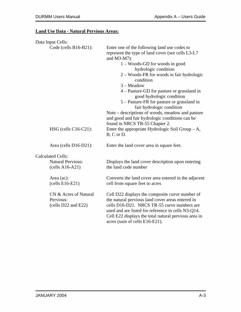
DURMM Users Manual Appendix A – Users Guide
JANUARY 2004 A-3
Land Use Data - Natural Pervious Areas: Data Input Cells:
Code (cells B16-B21): Enter one of the following land use codes to represent the type of land cover (see cells L3-L7 and M3-M7): 1 – Woods-GD for woods in good hydrologic condition 2 – Woods-FR for woods in fair hydrologic condition 3 – Meadow 4 – Pasture-GD for pasture or grassland in good hydrologic condition 5 – Pasture-FR for pasture or grassland in fair hydrologic condition Note – descriptions of woods, meadow and pasture and good and fair hydrologic conditions can be found in NRCS TR-55 Chapter 2. HSG (cells C16-C21): Enter the appropriate Hydrologic Soil Group – A, B, C or D. Area (cells D16-D21): Enter the land cover area in square feet.
Calculated Cells: Natural Pervious: Displays the land cover description upon entering (cells A16-A21) the land code number Area (ac): Converts the land cover area entered in the adjacent (cells E16-E21) cell from square feet to acres CN & Acres of Natural Cell D22 displays the composite curve number of Pervious: the natural pervious land cover areas entered in (cells D22 and E22) cells D16-D21. NRCS TR-55 curve numbers are used and are listed for reference in cells N3-Q14. Cell E22 displays the total natural pervious area in acres (sum of cells E16-E21).
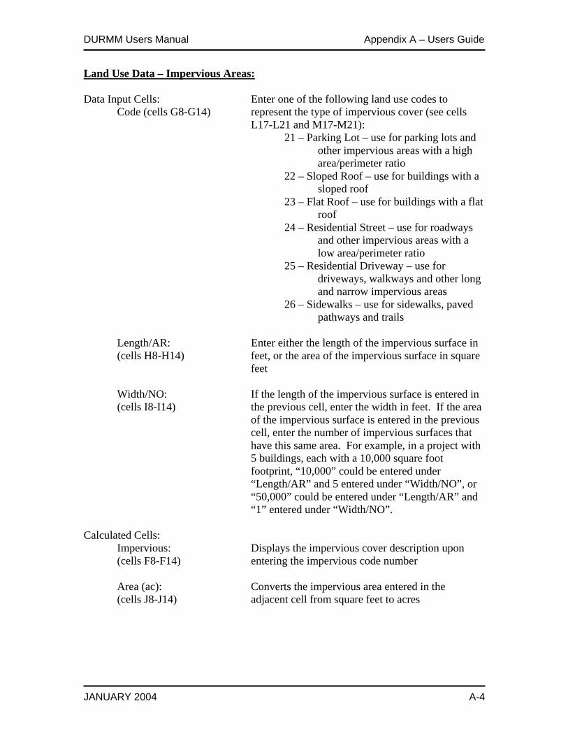
DURMM Users Manual Appendix A – Users Guide
JANUARY 2004 A-4
Land Use Data – Impervious Areas:
Data Input Cells: Enter one of the following land use codes to Code (cells G8-G14) represent the type of impervious cover (see cells L17-L21 and M17-M21): 21 – Parking Lot – use for parking lots and other impervious areas with a high area/perimeter ratio 22 – Sloped Roof – use for buildings with a sloped roof 23 – Flat Roof – use for buildings with a flat roof 24 – Residential Street – use for roadways and other impervious areas with a low area/perimeter ratio 25 – Residential Driveway – use for driveways, walkways and other long and narrow impervious areas 26 – Sidewalks – use for sidewalks, paved pathways and trails Length/AR: Enter either the length of the impervious surface in (cells H8-H14) feet, or the area of the impervious surface in square feet Width/NO: If the length of the impervious surface is entered in (cells I8-I14) the previous cell, enter the width in feet. If the area of the impervious surface is entered in the previous cell, enter the number of impervious surfaces that have this same area. For example, in a project with 5 buildings, each with a 10,000 square foot footprint, “10,000” could be entered under “Length/AR” and 5 entered under “Width/NO”, or “50,000” could be entered under “Length/AR” and “1” entered under “Width/NO”. Calculated Cells: Impervious: Displays the impervious cover description upon (cells F8-F14) entering the impervious code number Area (ac): Converts the impervious area entered in the (cells J8-J14) adjacent cell from square feet to acres
DURMM Users Manual Appendix A – Users Guide
JANUARY 2004 A-5
CN & Acres of Cell I15 displays the composite curve number of Impervious: the impervious areas entered in cells H8-I14. (cells I15 and J15) Curve numbers from the SLAMM Model are used and are listed for reference in cells N17-N21. Cell J15 displays the total impervious area in acres (sum of cells J8-J14).
Land Use Data – Total Site: Calculated Cells: Total Acreage: Displays the total site acreage, sum of the graded (cell H16) pervious area, natural pervious area and impervious area (cells E14, E22 and J15) % Impervious: Displays the percentage of the total site area that is (cell J16) impervious (cell J15 divided by cell H16) Disconnection Adjustments: Data Input Cells: Percent Impervious: Enter the percentage of the impervious area within (cell H18) the subarea that is disconnected. This value must be computed separately. Wetted Length: Enter the distance in feet along the edge of the (cell H19) impervious surface where runoff sheet flows onto the pervious surface. Wetted Width: Enter the distance in feet perpendicular to the edge (cell H20) of the impervious surface that effectively contributes to disconnection – use a maximum of 5 feet for concentrated flow, such as a downspout, and a maximum of 10 feet for sheet flow. Percent Flow Path: Enter the estimated percentage of the subarea’s total (cell H21) flow path that is used by runoff from the disconnected impervious area. Pervious CN: Enter the curve number of the pervious surface (cell H22) where the disconnected runoff flows off the impervious area onto the pervious area.
DURMM Users Manual Appendix A – Users Guide
JANUARY 2004 A-6
Calculated Cells: Overland Wetted Area: Displays the size of the sheet flow wetted pervious (cell J19) area (in acres) that is used for distributing the disconnected impervious runoff as excess rainfall – equal to the wetted length times the wetted width. Flow Path Wetted Area: Displays the size of the concentrated flow pervious (cell J20) area (in acres) that is used for distributing the disconnected impervious runoff as excess rainfall – equal to the swale flow bottom area located downstream of the disconnected impervious area. Total Wetted Area: Displays the sum of the overland wetted area and (cell J21) the flow path wetted area, in acres. % Impervious: Displays the total wetted area as a percentage of the (cell J22) total impervious area within the subarea. Runoff Volumes: Reference Cells: Rainfall Depths: Displays the 24-hour rainfall depths for the (cells C24-D27) quality (2 inch), bankfull (2-year), conveyance (10- year) and flooding (100-year) storm events. Except for the quality storm, these values vary by County. Calculated Cells: Natural Pervious Area Displays the runoff volume in cubic feet from the Runoff Volume: natural pervious area - as computed by NRCS (cells E24-E27) TR-20 routines. Graded Pervious Area Displays the runoff volume in cubic feet from the Runoff Volume: graded pervious area - as computed by DURMM (cells F24-F27) routines incorporating SLAMM equations for storm events less than 5 inches of rainfall, and NRCS TR-20 equations for storm events greater than 5 inches of rainfall.
DURMM Users Manual Appendix A – Users Guide
JANUARY 2004 A-7
Impervious Area Displays the unrouted runoff volume in cubic feet Runoff Volume: from the impervious area - as computed by (cells G24-G27) DURMM routines incorporating SLAMM equations for storm events less than 5 inches of rainfall, and NRCS TR-20 equations for storm events greater than 5 inches of rainfall. The runoff volumes computed here do not take into account the disconnection adjustments (i.e., they are “unrouted”). Routed Runoff Volume: Displays the sum of the runoff volumes from (cells H24-H27) natural pervious area, graded pervious area and routed impervious area, in cubic feet. The impervious area runoff volumes used in this calculation take into account the disconnection routines, even though the previous column (cells G24-G27) displays the impervious area runoff volumes with no disconnection. To determine the disconnected impervious runoff volume for each storm event, subtract the natural and graded area volumes from the routed total volume. Reduction in Runoff Displays the reduction in total runoff volume due to Volume: impervious area disconnection – the routed runoff (cells I24-I27) volume (column H) divided by the sum of the natural, graded and unrouted pervious runoff volumes (columns E, F and G), expressed as a percentage. Runoff (in.): Displays the runoff depth in inches - the routed (cells J24-J27) runoff volume divided by the subarea size. Flow Path Data: Data Input Cells: Sheet Flow Parameters: Length: Enter the length in feet of the upper (cell B30) and (cells B30-B31) lower (cell B31) sheet flow segments of the flow path. Leave both cells blank if the subarea has no sheet flow, leave cell B31 blank if there is only one sheet flow segment.
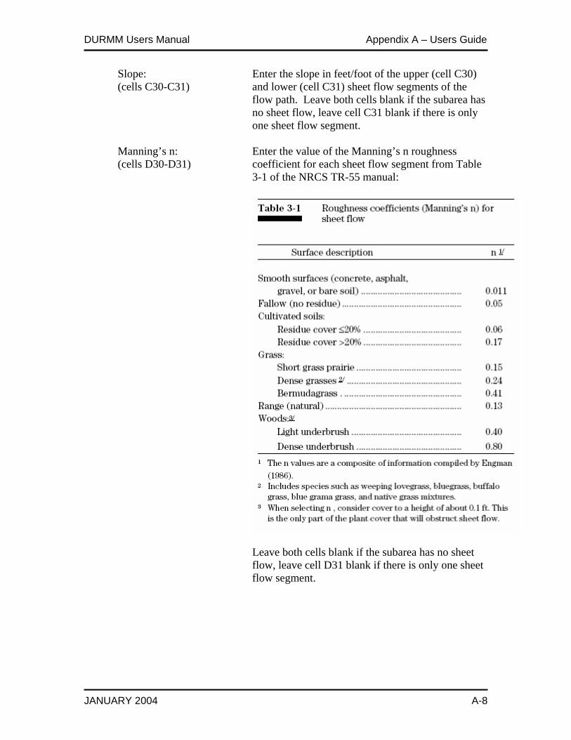
DURMM Users Manual Appendix A – Users Guide
JANUARY 2004 A-8
Slope: Enter the slope in feet/foot of the upper (cell C30) (cells C30-C31) and lower (cell C31) sheet flow segments of the flow path. Leave both cells blank if the subarea has no sheet flow, leave cell C31 blank if there is only one sheet flow segment. Manning’s n: Enter the value of the Manning’s n roughness (cells D30-D31) coefficient for each sheet flow segment from Table 3-1 of the NRCS TR-55 manual:
Leave both cells blank if the subarea has no sheet flow, leave cell D31 blank if there is only one sheet flow segment.
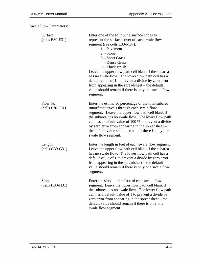
DURMM Users Manual Appendix A – Users Guide
JANUARY 2004 A-9
Swale Flow Parameters: Surface: Enter one of the following surface codes to (cells E30-E31) represent the surface cover of each swale flow segment (see cells L33-M37): 1 – Pavement 2 – Stone 3 – Short Grass 4 – Dense Grass 5 – Thick Brush Leave the upper flow path cell blank if the subarea has no swale flow. The lower flow path cell has a default value of 1 to prevent a divide by zero error from appearing in the spreadsheet – the default value should remain if there is only one swale flow segment. Flow %: Enter the estimated percentage of the total subarea (cells F30-F31) runoff that travels through each swale flow segment. Leave the upper flow path cell blank if the subarea has no swale flow. The lower flow path cell has a default value of 100 % to prevent a divide by zero error from appearing in the spreadsheet – the default value should remain if there is only one swale flow segment. Length: Enter the length in feet of each swale flow segment. (cells G30-G31) Leave the upper flow path cell blank if the subarea has no swale flow. The lower flow path cell has a default value of 1 to prevent a divide by zero error from appearing in the spreadsheet – the default value should remain if there is only one swale flow segment. Slope: Enter the slope in feet/foot of each swale flow (cells H30-H31) segment. Leave the upper flow path cell blank if the subarea has no swale flow. The lower flow path cell has a default value of 1 to prevent a divide by zero error from appearing in the spreadsheet – the default value should remain if there is only one swale flow segment.
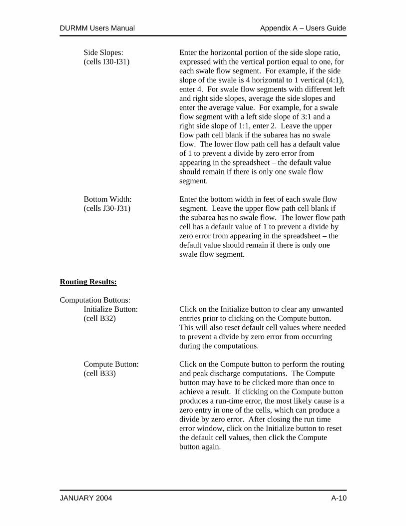
DURMM Users Manual Appendix A – Users Guide
JANUARY 2004 A-10
Side Slopes: Enter the horizontal portion of the side slope ratio, (cells I30-I31) expressed with the vertical portion equal to one, for each swale flow segment. For example, if the side slope of the swale is 4 horizontal to 1 vertical (4:1), enter 4. For swale flow segments with different left and right side slopes, average the side slopes and enter the average value. For example, for a swale flow segment with a left side slope of 3:1 and a right side slope of 1:1, enter 2. Leave the upper flow path cell blank if the subarea has no swale flow. The lower flow path cell has a default value of 1 to prevent a divide by zero error from appearing in the spreadsheet – the default value should remain if there is only one swale flow segment. Bottom Width: Enter the bottom width in feet of each swale flow (cells J30-J31) segment. Leave the upper flow path cell blank if the subarea has no swale flow. The lower flow path cell has a default value of 1 to prevent a divide by zero error from appearing in the spreadsheet – the default value should remain if there is only one swale flow segment. Routing Results: Computation Buttons: Initialize Button: Click on the Initialize button to clear any unwanted (cell B32) entries prior to clicking on the Compute button. This will also reset default cell values where needed to prevent a divide by zero error from occurring during the computations. Compute Button: Click on the Compute button to perform the routing (cell B33) and peak discharge computations. The Compute button may have to be clicked more than once to achieve a result. If clicking on the Compute button produces a run-time error, the most likely cause is a zero entry in one of the cells, which can produce a divide by zero error. After closing the run time error window, click on the Initialize button to reset the default cell values, then click the Compute button again.
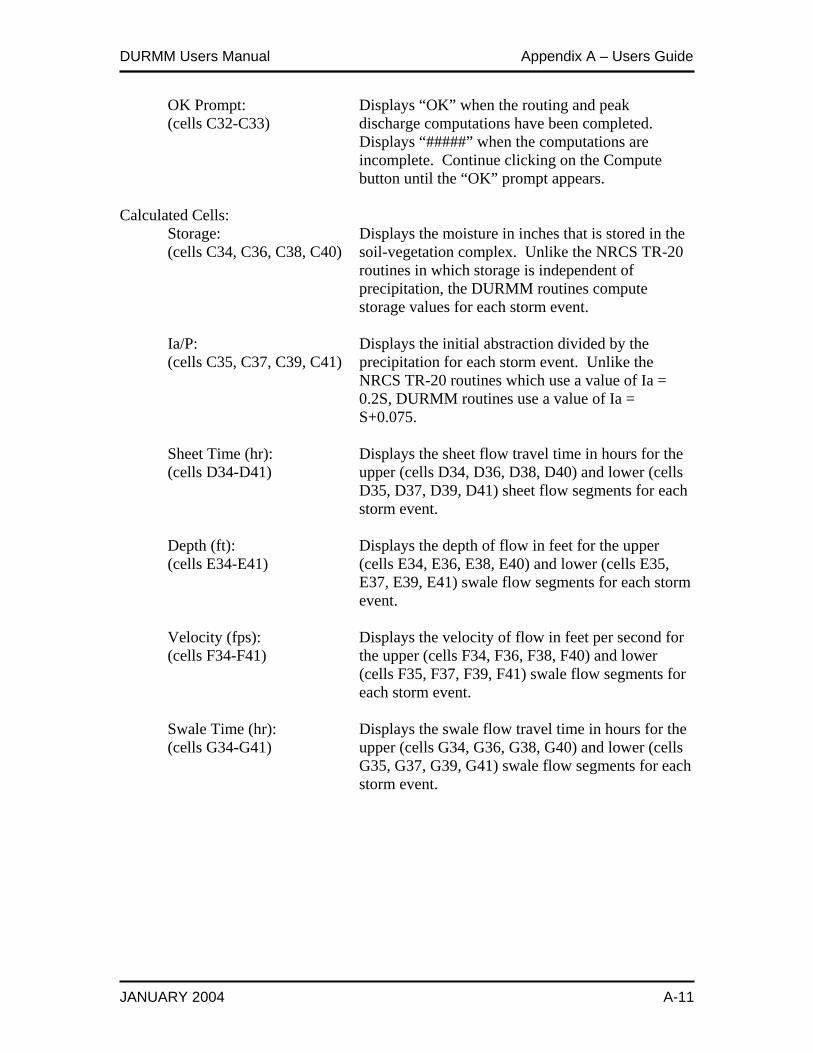
DURMM Users Manual Appendix A – Users Guide
JANUARY 2004 A-11
OK Prompt: Displays “OK” when the routing and peak (cells C32-C33) discharge computations have been completed. Displays “#####” when the computations are incomplete. Continue clicking on the Compute button until the “OK” prompt appears. Calculated Cells: Storage: Displays the moisture in inches that is stored in the (cells C34, C36, C38, C40) soil-vegetation complex. Unlike the NRCS TR-20 routines in which storage is independent of precipitation, the DURMM routines compute storage values for each storm event. Ia/P: Displays the initial abstraction divided by the (cells C35, C37, C39, C41) precipitation for each storm event. Unlike the NRCS TR-20 routines which use a value of Ia = 0.2S, DURMM routines use a value of Ia = S+0.075. Sheet Time (hr): Displays the sheet flow travel time in hours for the (cells D34-D41) upper (cells D34, D36, D38, D40) and lower (cells D35, D37, D39, D41) sheet flow segments for each storm event. Depth (ft): Displays the depth of flow in feet for the upper (cells E34-E41) (cells E34, E36, E38, E40) and lower (cells E35, E37, E39, E41) swale flow segments for each storm event. Velocity (fps): Displays the velocity of flow in feet per second for (cells F34-F41) the upper (cells F34, F36, F38, F40) and lower (cells F35, F37, F39, F41) swale flow segments for each storm event. Swale Time (hr): Displays the swale flow travel time in hours for the (cells G34-G41) upper (cells G34, G36, G38, G40) and lower (cells G35, G37, G39, G41) swale flow segments for each storm event.
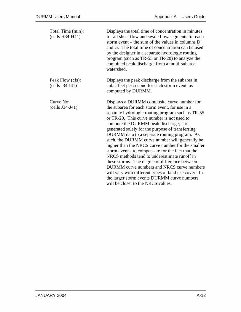
DURMM Users Manual Appendix A – Users Guide
JANUARY 2004 A-12
Total Time (min): Displays the total time of concentration in minutes (cells H34-H41) for all sheet flow and swale flow segments for each storm event – the sum of the values in columns D and G. The total time of concentration can be used by the designer in a separate hydrologic routing program (such as TR-55 or TR-20) to analyze the combined peak discharge from a multi-subarea watershed. Peak Flow (cfs): Displays the peak discharge from the subarea in (cells I34-I41) cubic feet per second for each storm event, as computed by DURMM. Curve No: Displays a DURMM composite curve number for (cells J34-J41) the subarea for each storm event, for use in a separate hydrologic routing program such as TR-55 or TR-20. This curve number is not used to compute the DURMM peak discharge; it is generated solely for the purpose of transferring DURMM data to a separate routing program. As such, the DURMM curve number will generally be higher than the NRCS curve number for the smaller storm events, to compensate for the fact that the NRCS methods tend to underestimate runoff in these storms. The degree of difference between DURMM curve numbers and NRCS curve numbers will vary with different types of land use cover. In the larger storm events DURMM curve numbers will be closer to the NRCS values.
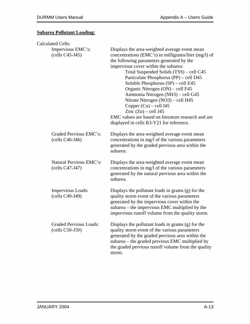
DURMM Users Manual Appendix A – Users Guide
JANUARY 2004 A-13
Subarea Pollutant Loading: Calculated Cells: Impervious EMC’s: Displays the area-weighted average event mean (cells C45-J45) concentrations (EMC’s) in milligrams/liter (mg/l) of the following parameters generated by the impervious cover within the subarea: Total Suspended Solids (TSS) – cell C45 Particulate Phosphorus (PP) – cell D45 Soluble Phosphorus (SP) – cell E45 Organic Nitrogen (ON) – cell F45 Ammonia Nitrogen (NH3) – cell G45 Nitrate Nitrogen (NO3) – cell H45 Copper (Cu) – cell I45 Zinc (Zn) – cell J45 EMC values are based on literature research and are displayed in cells R3-Y21 for reference. Graded Pervious EMC’s: Displays the area-weighted average event mean (cells C46-J46) concentrations in mg/l of the various parameters generated by the graded pervious area within the subarea. Natural Pervious EMC’s: Displays the area-weighted average event mean (cells C47-J47) concentrations in mg/l of the various parameters generated by the natural pervious area within the subarea. Impervious Loads: Displays the pollutant loads in grams (g) for the (cells C49-J49) quality storm event of the various parameters generated by the impervious cover within the subarea – the impervious EMC multiplied by the impervious runoff volume from the quality storm. Graded Pervious Loads: Displays the pollutant loads in grams (g) for the (cells C50-J50) quality storm event of the various parameters generated by the graded pervious area within the subarea – the graded pervious EMC multiplied by the graded pervious runoff volume from the quality storm.
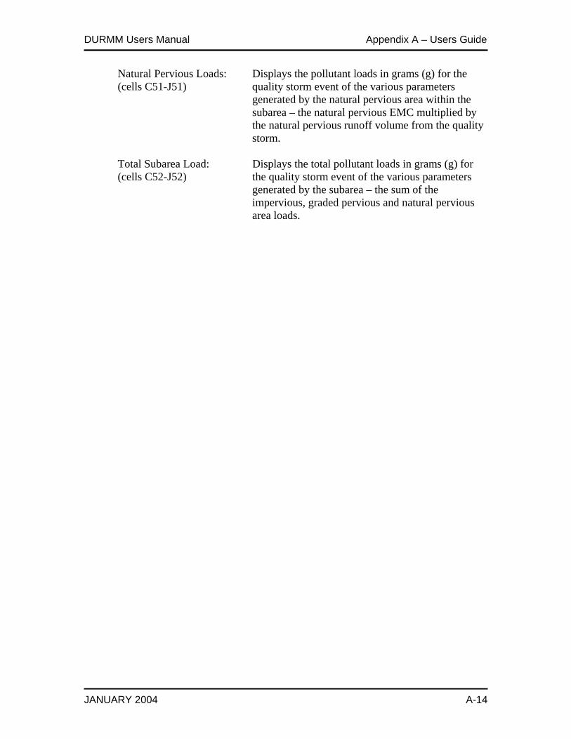
DURMM Users Manual Appendix A – Users Guide
JANUARY 2004 A-14
Natural Pervious Loads: Displays the pollutant loads in grams (g) for the (cells C51-J51) quality storm event of the various parameters generated by the natural pervious area within the subarea – the natural pervious EMC multiplied by the natural pervious runoff volume from the quality storm. Total Subarea Load: Displays the total pollutant loads in grams (g) for (cells C52-J52) the quality storm event of the various parameters generated by the subarea – the sum of the impervious, graded pervious and natural pervious area loads.
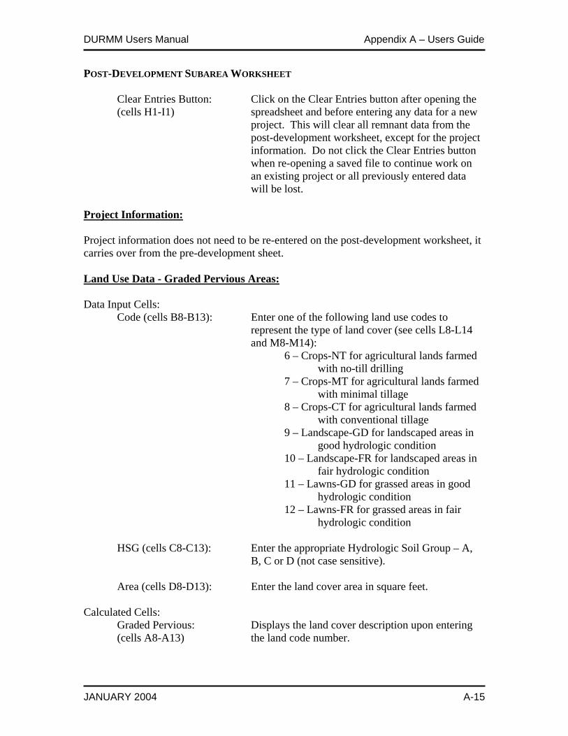
DURMM Users Manual Appendix A – Users Guide
JANUARY 2004 A-15
POST-DEVELOPMENT SUBAREA WORKSHEET Clear Entries Button: Click on the Clear Entries button after opening the (cells H1-I1) spreadsheet and before entering any data for a new project. This will clear all remnant data from the post-development worksheet, except for the project information. Do not click the Clear Entries button when re-opening a saved file to continue work on an existing project or all previously entered data will be lost. Project Information: Project information does not need to be re-entered on the post-development worksheet, it carries over from the pre-development sheet. Land Use Data - Graded Pervious Areas: Data Input Cells:
Code (cells B8-B13): Enter one of the following land use codes to represent the type of land cover (see cells L8-L14 and M8-M14): 6 – Crops-NT for agricultural lands farmed with no-till drilling 7 – Crops-MT for agricultural lands farmed with minimal tillage 8 – Crops-CT for agricultural lands farmed with conventional tillage 9 – Landscape-GD for landscaped areas in good hydrologic condition 10 – Landscape-FR for landscaped areas in fair hydrologic condition 11 – Lawns-GD for grassed areas in good hydrologic condition 12 – Lawns-FR for grassed areas in fair hydrologic condition HSG (cells C8-C13): Enter the appropriate Hydrologic Soil Group – A, B, C or D (not case sensitive). Area (cells D8-D13): Enter the land cover area in square feet.
Calculated Cells: Graded Pervious: Displays the land cover description upon entering (cells A8-A13) the land code number.
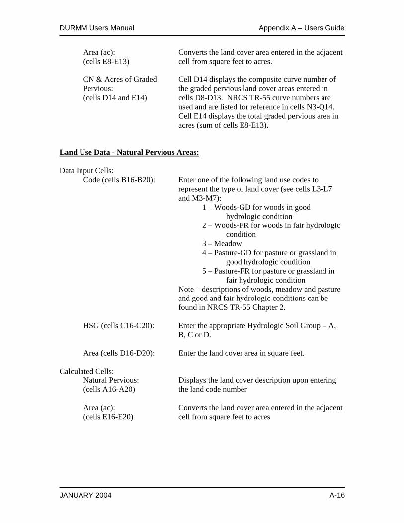
DURMM Users Manual Appendix A – Users Guide
JANUARY 2004 A-16
Area (ac): Converts the land cover area entered in the adjacent (cells E8-E13) cell from square feet to acres. CN & Acres of Graded Cell D14 displays the composite curve number of Pervious: the graded pervious land cover areas entered in (cells D14 and E14) cells D8-D13. NRCS TR-55 curve numbers are used and are listed for reference in cells N3-Q14. Cell E14 displays the total graded pervious area in acres (sum of cells E8-E13).
Land Use Data - Natural Pervious Areas: Data Input Cells:
Code (cells B16-B20): Enter one of the following land use codes to represent the type of land cover (see cells L3-L7 and M3-M7): 1 – Woods-GD for woods in good hydrologic condition 2 – Woods-FR for woods in fair hydrologic condition 3 – Meadow 4 – Pasture-GD for pasture or grassland in good hydrologic condition 5 – Pasture-FR for pasture or grassland in fair hydrologic condition Note – descriptions of woods, meadow and pasture and good and fair hydrologic conditions can be found in NRCS TR-55 Chapter 2. HSG (cells C16-C20): Enter the appropriate Hydrologic Soil Group – A, B, C or D. Area (cells D16-D20): Enter the land cover area in square feet.
Calculated Cells: Natural Pervious: Displays the land cover description upon entering (cells A16-A20) the land code number Area (ac): Converts the land cover area entered in the adjacent (cells E16-E20) cell from square feet to acres
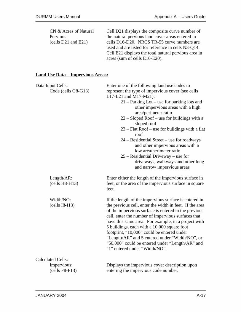
DURMM Users Manual Appendix A – Users Guide
JANUARY 2004 A-17
CN & Acres of Natural Cell D21 displays the composite curve number of Pervious: the natural pervious land cover areas entered in (cells D21 and E21) cells D16-D20. NRCS TR-55 curve numbers are used and are listed for reference in cells N3-Q14. Cell E21 displays the total natural pervious area in acres (sum of cells E16-E20).
Land Use Data – Impervious Areas:
Data Input Cells: Enter one of the following land use codes to Code (cells G8-G13) represent the type of impervious cover (see cells L17-L21 and M17-M21): 21 – Parking Lot – use for parking lots and other impervious areas with a high area/perimeter ratio 22 – Sloped Roof – use for buildings with a sloped roof 23 – Flat Roof – use for buildings with a flat roof 24 – Residential Street – use for roadways and other impervious areas with a low area/perimeter ratio 25 – Residential Driveway – use for driveways, walkways and other long and narrow impervious areas Length/AR: Enter either the length of the impervious surface in (cells H8-H13) feet, or the area of the impervious surface in square feet. Width/NO: If the length of the impervious surface is entered in (cells I8-I13) the previous cell, enter the width in feet. If the area of the impervious surface is entered in the previous cell, enter the number of impervious surfaces that have this same area. For example, in a project with 5 buildings, each with a 10,000 square foot footprint, “10,000” could be entered under “Length/AR” and 5 entered under “Width/NO”, or “50,000” could be entered under “Length/AR” and “1” entered under “Width/NO”. Calculated Cells: Impervious: Displays the impervious cover description upon (cells F8-F13) entering the impervious code number.

DURMM Users Manual Appendix A – Users Guide
JANUARY 2004 A-18
Area (ac): Converts the impervious area entered in the (cells J8-J13) adjacent cell from square feet to acres.
CN & Acres of Cell I14 displays the composite curve number of Impervious: the impervious areas entered in cells H8-I13. (cells I14 and J14) Curve numbers from the SLAMM Model are used and are listed for reference in cells N17-N21. Cell J14 displays the total impervious area in acres (sum of cells J8-J13).
Land Use Data – Total Site: Calculated Cells: Total Acreage: Displays the total site acreage, sum of the graded (cell H15) pervious area, natural pervious area and impervious area (cells E14, E21 and J14). % Impervious: Displays the percentage of the total site area that is (cell J15) impervious (cell J14 divided by cell H15). Disconnection Adjustments: Data Input Cells: Percent Impervious: Enter the percentage of the impervious area within (cell H17) the subarea that is disconnected. This value must be computed separately. Wetted Length: Enter the distance in feet along the edge of the (cell H18) impervious surface where runoff sheet flows onto the pervious surface. Wetted Width: Enter the distance in feet perpendicular to the edge (cell H19) of the impervious surface that effectively contributes to disconnection – use a maximum of 5 feet for concentrated flow, such as a downspout, and a maximum of 10 feet for sheet flow. Percent Flow Path: Enter the estimated percentage of the subarea’s total (cell H20) flow path that is used by runoff from the disconnected impervious area. Pervious CN: Enter the curve number of the pervious surface (cell H21) where the disconnected runoff flows off the impervious area onto the pervious area.
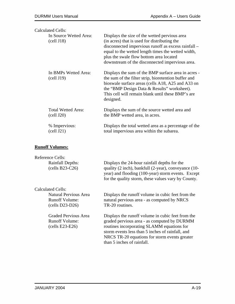
DURMM Users Manual Appendix A – Users Guide
JANUARY 2004 A-19
Calculated Cells: In Source Wetted Area: Displays the size of the wetted pervious area (cell J18) (in acres) that is used for distributing the disconnected impervious runoff as excess rainfall – equal to the wetted length times the wetted width, plus the swale flow bottom area located downstream of the disconnected impervious area. In BMPs Wetted Area: Displays the sum of the BMP surface area in acres - (cell J19) the sum of the filter strip, bioretention buffer and bioswale surface areas (cells A18, A25 and A33 on the “BMP Design Data & Results” worksheet). This cell will remain blank until these BMP’s are designed. Total Wetted Area: Displays the sum of the source wetted area and (cell J20) the BMP wetted area, in acres. % Impervious: Displays the total wetted area as a percentage of the (cell J21) total impervious area within the subarea. Runoff Volumes: Reference Cells: Rainfall Depths: Displays the 24-hour rainfall depths for the (cells B23-C26) quality (2 inch), bankfull (2-year), conveyance (10- year) and flooding (100-year) storm events. Except for the quality storm, these values vary by County. Calculated Cells: Natural Pervious Area Displays the runoff volume in cubic feet from the Runoff Volume: natural pervious area - as computed by NRCS (cells D23-D26) TR-20 routines. Graded Pervious Area Displays the runoff volume in cubic feet from the Runoff Volume: graded pervious area - as computed by DURMM (cells E23-E26) routines incorporating SLAMM equations for storm events less than 5 inches of rainfall, and NRCS TR-20 equations for storm events greater than 5 inches of rainfall.
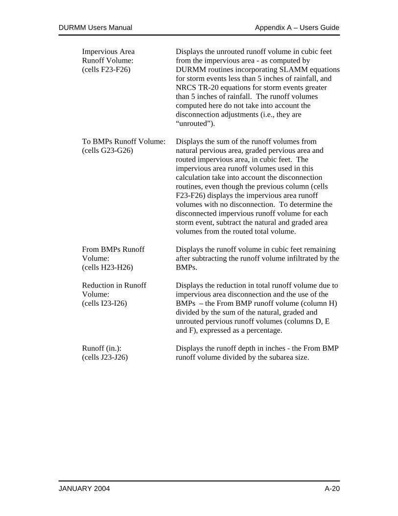
DURMM Users Manual Appendix A – Users Guide
JANUARY 2004 A-20
Impervious Area Displays the unrouted runoff volume in cubic feet Runoff Volume: from the impervious area - as computed by (cells F23-F26) DURMM routines incorporating SLAMM equations for storm events less than 5 inches of rainfall, and NRCS TR-20 equations for storm events greater than 5 inches of rainfall. The runoff volumes computed here do not take into account the disconnection adjustments (i.e., they are “unrouted”). To BMPs Runoff Volume: Displays the sum of the runoff volumes from (cells G23-G26) natural pervious area, graded pervious area and routed impervious area, in cubic feet. The impervious area runoff volumes used in this calculation take into account the disconnection routines, even though the previous column (cells F23-F26) displays the impervious area runoff volumes with no disconnection. To determine the disconnected impervious runoff volume for each storm event, subtract the natural and graded area volumes from the routed total volume. From BMPs Runoff Displays the runoff volume in cubic feet remaining Volume: after subtracting the runoff volume infiltrated by the (cells H23-H26) BMPs. Reduction in Runoff Displays the reduction in total runoff volume due to Volume: impervious area disconnection and the use of the (cells I23-I26) BMPs – the From BMP runoff volume (column H) divided by the sum of the natural, graded and unrouted pervious runoff volumes (columns D, E and F), expressed as a percentage. Runoff (in.): Displays the runoff depth in inches - the From BMP (cells J23-J26) runoff volume divided by the subarea size.
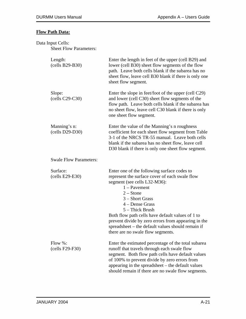
DURMM Users Manual Appendix A – Users Guide
JANUARY 2004 A-21
Flow Path Data: Data Input Cells: Sheet Flow Parameters: Length: Enter the length in feet of the upper (cell B29) and (cells B29-B30) lower (cell B30) sheet flow segments of the flow path. Leave both cells blank if the subarea has no sheet flow, leave cell B30 blank if there is only one sheet flow segment. Slope: Enter the slope in feet/foot of the upper (cell C29) (cells C29-C30) and lower (cell C30) sheet flow segments of the flow path. Leave both cells blank if the subarea has no sheet flow, leave cell C30 blank if there is only one sheet flow segment. Manning’s n: Enter the value of the Manning’s n roughness (cells D29-D30) coefficient for each sheet flow segment from Table 3-1 of the NRCS TR-55 manual. Leave both cells blank if the subarea has no sheet flow, leave cell D30 blank if there is only one sheet flow segment. Swale Flow Parameters: Surface: Enter one of the following surface codes to (cells E29-E30) represent the surface cover of each swale flow segment (see cells L32-M36): 1 – Pavement 2 – Stone 3 – Short Grass 4 – Dense Grass 5 – Thick Brush Both flow path cells have default values of 1 to prevent divide by zero errors from appearing in the spreadsheet – the default values should remain if there are no swale flow segments. Flow %: Enter the estimated percentage of the total subarea (cells F29-F30) runoff that travels through each swale flow segment. Both flow path cells have default values of 100% to prevent divide by zero errors from appearing in the spreadsheet – the default values should remain if there are no swale flow segments.

DURMM Users Manual Appendix A – Users Guide
JANUARY 2004 A-22
Length: Enter the length in feet of each swale flow segment. (cells G29-G30) Both flow path cells have default values of 1 to prevent divide by zero errors from appearing in the spreadsheet – the default values should remain if there are no swale flow segments. Slope: Enter the slope in feet/foot of each swale flow (cells H29-H30) segment. Both flow path cells have default values of 1 to prevent divide by zero errors from appearing in the spreadsheet – the default values should remain if there are no swale flow segments. Side Slopes: Enter the horizontal portion of the side slope ratio, (cells I29-I30) expressed with the vertical portion equal to one, for each swale flow segment. For example, if the side slope of the swale is 4 horizontal to 1 vertical (4:1), enter 4. For swale flow segments with different left and right side slopes, average the side slopes and enter the average value. For example, for a swale flow segment with a left side slope of 3:1 and a right side slope of 1:1, enter 2. Both flow path cells have default values of 1 to prevent divide by zero errors from appearing in the spreadsheet – the default values should remain if there are no swale flow segments. Bottom Width: Enter the bottom width in feet of each swale flow (cells J29-J30) segment. Both flow path cells have default values of 1 to prevent divide by zero errors from appearing in the spreadsheet – the default values should remain if there are no swale flow segments. Calculated Cells: % Runoff Impervious: Displays the percentage of the total runoff volume (cell B31) in the quality storm that is generated by the impervious area – the impervious area runoff volume divided by the total runoff volume, expressed as a percentage, not taking into account disconnection or runoff infiltrated by BMPs.
DURMM Users Manual Appendix A – Users Guide
JANUARY 2004 A-23
Tc Path: Displays “IMPERV” if greater than 45% of the (cell D31) quality storm runoff volume is generated by impervious areas and “PERVIOUS” if less than 45% of the quality storm runoff volume is generated by impervious areas. This cell should be used as a check by the designer to verify that the selected Tc path is appropriate – if the runoff volume is predominately from the impervious area (“IMPERV”) than the Tc path should be through the impervious area, not across a pervious area. Cells E31-J31: If a bioswale is designed on the “BMP Design Data & Results” worksheet, the bioswale design parameters are repeated in these cells as follows: Cell E31 – bioswale surface code Cell F31 – bioswale flow percentage Cell G31 – bioswale length Cell H31 – bioswale slope Cell I31 – bioswale side slope Cell J31 – bioswale bottom width These cells remain blank or have a default value of 1 if a bioswale is not used as part of the design. The default value of 1 is used in certain cells to prevent a divide by zero error from appearing in the spreadsheet. Routing Results: Computation Buttons: Initialize Button: Click on the Initialize button to clear any unwanted (cell B32) entries prior to clicking on the Compute button. This will also reset default cell values where needed to prevent a divide by zero error from occurring during the computations. Compute Button: Click on the Compute button to perform the routing (cell B33) and peak discharge computations. The Compute button may have to be clicked more than once to achieve a result. If clicking on the Compute button produces a run-time error, the most likely cause is a zero entry in one of the cells, which can produce a divide by zero error. After closing the run time error window, click on the Initialize button to reset the default cell values, then click the Compute button again.
DURMM Users Manual Appendix A – Users Guide
JANUARY 2004 A-24
OK Prompt: Displays “OK” when the routing and peak (cells C32-C33) discharge computations have been completed. Displays “#####” when the computations are incomplete. Continue clicking on the Compute button until the “OK” prompt appears. Calculated Cells: Storage: Displays the moisture in inches that is stored in the (cells C34, C37, C40, C43) soil-vegetation complex. Unlike the NRCS TR-20 routines in which storage is independent of precipitation, the DURMM routines compute storage values for each storm event. Ia/P: Displays the initial abstraction divided by the (cells C35, C38, C41, C44) precipitation for each storm event. Unlike the NRCS TR-20 routines which use a value of Ia = 0.2S, DURMM routines use a value of Ia = S+0.075. Sheet Time (hr): Displays the sheet flow travel time in hours for the (cells D34-D44) upper (cells D34, D37, D40, D43) and lower (cells D35, D38, D41, D44) sheet flow segments for each storm event. Depth (ft): Displays the depth of flow in feet for the upper (cells E34-E45) (cells E34, E37, E40, E43) and lower (cells E35, E38, E41, E44) swale flow segments for each storm event. If a bioswale is designed on the “BMP Design Data & Results” worksheet, the bioswale flow depths, in feet, are displayed in cells E36, E39, E42 and E45. If a bioswale is not used in the design, these cells display varying default values to prevent divide by zero errors from appearing in the spreadsheet. Velocity (fps): Displays the velocity of flow in feet per second for (cells F34-F45) the upper (cells F34, F37, F40, F43) and lower (cells F35, F38, F41, F44) swale flow segments for each storm event. If a bioswale is designed on the “BMP Design Data & Results” worksheet, the bioswale velocities, in feet per second, are displayed in cells F36, F39, F42 and F45. If a bioswale is not used in the design, these cells display varying default values to prevent divide by zero errors from appearing in the spreadsheet.
DURMM Users Manual Appendix A – Users Guide
JANUARY 2004 A-25
Swale Time (hr): Displays the swale flow travel time in hours for the (cells G34-G45) upper (cells G34, G37, G40, G43) and lower (cells G35, G38, G41, G44) swale flow segments for each storm event. If a bioswale is designed on the “BMP Design Data & Results” worksheet, the bioswale travel times, in hours, are displayed in cells G36, G39, G42 and G45. If a bioswale is not used in the design, these cells remain blank. Total Time (min): Cells H34/35, H37/38, H40/41 and H43/44 display (cells H34-H45) the total time of concentration in minutes for all sheet flow and swale flow segments for each storm event – the sum of the values in columns D and G. If a bioswale is designed on the “BMP Design Data & Results” worksheet, the times of concentration displayed in cells H36, H39, H42 and H45 include the travel time in the bioswale. If a bioswale is not used, these cells display the same values as the adjacent cells. The total time of concentration can be used by the designer in a separate hydrologic routing program (such as TR-55 or TR-20) to analyze the combined peak discharge from a multi- subarea watershed. Peak Flow (cfs): Cells I34/35, I37/38, I40/41 and I43/44 display the (cells I34-I45) peak discharge from the subarea in cubic feet per second for each storm event, as computed by DURMM. If a bioswale is designed on the “BMP Design Data & Results” worksheet, the values displayed in cells I36, I39, I42 and I45 represent the peak discharges after flows are routed through the bioswale. If a bioswale is not used, these cells display the same values as the adjacent cells.
DURMM Users Manual Appendix A – Users Guide
JANUARY 2004 A-26
Curve No: Displays a DURMM composite curve number for (cells J34/35, J37/38, the subarea for each storm event, for use in a J40/41 and J43/44) separate hydrologic routing program such as TR-55 or TR-20. This curve number is not used to compute the DURMM peak discharge; it is generated solely for the purpose of transferring DURMM data to a separate routing program. As such, the DURMM curve number will generally be higher than the NRCS curve number for the smaller storm events, to compensate for the fact that the NRCS methods tend to underestimate runoff in these storms. The degree of difference between DURMM curve numbers and NRCS curve numbers will vary with different types of land use cover. In the larger storm events DURMM curve numbers will be closer to the NRCS values. Cells J36, J39, J42 and J45: If a bioswale is designed on the “BMP Design Data & Results” worksheet, the values displayed in these cells represent the reduction in peak discharge due to routing through the bioswale for each storm event. If a bioswale is not used these cells remain blank. Subarea Pollutant Loading: Calculated Cells: Impervious EMC’s: Displays the area-weighted average event mean (cells C48-J48) concentrations (EMC’s) in milligrams/liter (mg/l) of the following parameters generated by the impervious cover within the subarea: Total Suspended Solids (TSS) – cell C48 Particulate Phosphorus (PP) – cell D48 Soluble Phosphorus (SP) – cell E48 Organic Nitrogen (ON) – cell F48 Ammonia Nitrogen (NH3) – cell G48 Nitrate Nitrogen (NO3) – cell H48 Copper (Cu) – cell I48 Zinc (Zn) – cell J48 EMC values are based on literature research and are displayed in cells R3-Y21for reference.
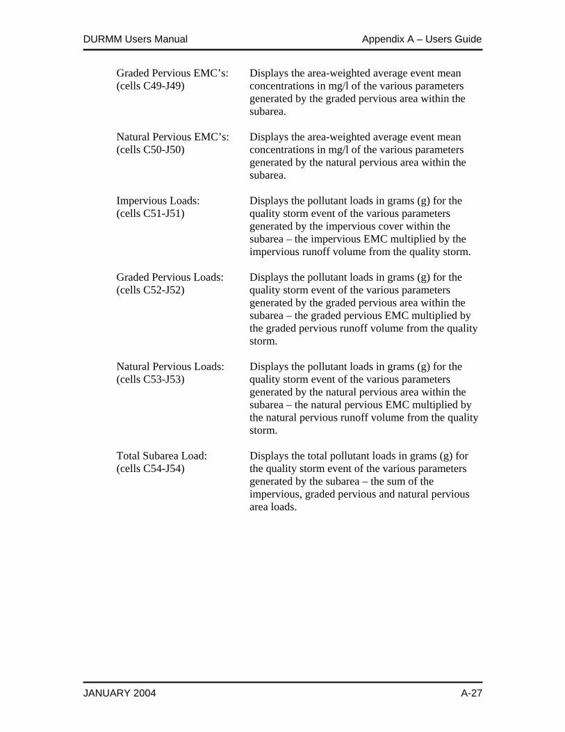
DURMM Users Manual Appendix A – Users Guide
JANUARY 2004 A-27
Graded Pervious EMC’s: Displays the area-weighted average event mean (cells C49-J49) concentrations in mg/l of the various parameters generated by the graded pervious area within the subarea. Natural Pervious EMC’s: Displays the area-weighted average event mean (cells C50-J50) concentrations in mg/l of the various parameters generated by the natural pervious area within the subarea. Impervious Loads: Displays the pollutant loads in grams (g) for the (cells C51-J51) quality storm event of the various parameters generated by the impervious cover within the subarea – the impervious EMC multiplied by the impervious runoff volume from the quality storm. Graded Pervious Loads: Displays the pollutant loads in grams (g) for the (cells C52-J52) quality storm event of the various parameters generated by the graded pervious area within the subarea – the graded pervious EMC multiplied by the graded pervious runoff volume from the quality storm. Natural Pervious Loads: Displays the pollutant loads in grams (g) for the (cells C53-J53) quality storm event of the various parameters generated by the natural pervious area within the subarea – the natural pervious EMC multiplied by the natural pervious runoff volume from the quality storm. Total Subarea Load: Displays the total pollutant loads in grams (g) for (cells C54-J54) the quality storm event of the various parameters generated by the subarea – the sum of the impervious, graded pervious and natural pervious area loads.
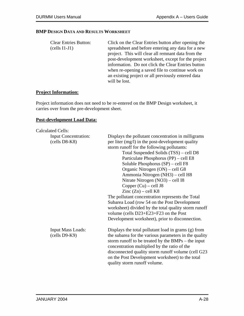
DURMM Users Manual Appendix A – Users Guide
JANUARY 2004 A-28
BMP DESIGN DATA AND RESULTS WORKSHEET Clear Entries Button: Click on the Clear Entries button after opening the (cells I1-J1) spreadsheet and before entering any data for a new project. This will clear all remnant data from the post-development worksheet, except for the project information. Do not click the Clear Entries button when re-opening a saved file to continue work on an existing project or all previously entered data will be lost. Project Information: Project information does not need to be re-entered on the BMP Design worksheet, it carries over from the pre-development sheet. Post-development Load Data: Calculated Cells: Input Concentration: Displays the pollutant concentration in milligrams (cells D8-K8) per liter (mg/l) in the post-development quality storm runoff for the following pollutants: Total Suspended Solids (TSS) – cell D8 Particulate Phosphorus (PP) – cell E8 Soluble Phosphorus (SP) – cell F8 Organic Nitrogen (ON) – cell G8 Ammonia Nitrogen (NH3) – cell H8 Nitrate Nitrogen (NO3) – cell I8 Copper (Cu) – cell J8 Zinc (Zn) – cell K8 The pollutant concentration represents the Total Subarea Load (row 54 on the Post Development worksheet) divided by the total quality storm runoff volume (cells D23+E23+F23 on the Post Development worksheet), prior to disconnection. Input Mass Loads: Displays the total pollutant load in grams (g) from (cells D9-K9) the subarea for the various parameters in the quality storm runoff to be treated by the BMPs – the input concentration multiplied by the ratio of the disconnected quality storm runoff volume (cell G23 on the Post Development worksheet) to the total quality storm runoff volume.
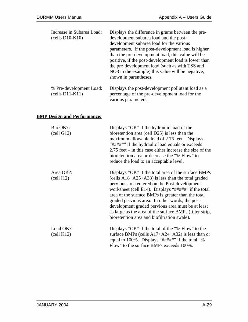
DURMM Users Manual Appendix A – Users Guide
JANUARY 2004 A-29
Increase in Subarea Load: Displays the difference in grams between the pre- (cells D10-K10) development subarea load and the post- development subarea load for the various parameters. If the post-development load is higher than the pre-development load, this value will be positive, if the post-development load is lower than the pre-development load (such as with TSS and NO3 in the example) this value will be negative, shown in parentheses. % Pre-development Load: Displays the post-development pollutant load as a (cells D11-K11) percentage of the pre-development load for the various parameters. BMP Design and Performance: Bio OK?: Displays “OK” if the hydraulic load of the (cell G12) bioretention area (cell D25) is less than the maximum allowable load of 2.75 feet. Displays “#####” if the hydraulic load equals or exceeds 2.75 feet – in this case either increase the size of the bioretention area or decrease the “% Flow” to reduce the load to an acceptable level. Area OK?: Displays “OK” if the total area of the surface BMPs (cell I12) (cells A18+A25+A33) is less than the total graded pervious area entered on the Post-development worksheet (cell E14). Displays “#####” if the total area of the surface BMPs is greater than the total graded pervious area. In other words, the post- development graded pervious area must be at least as large as the area of the surface BMPs (filter strip, bioretention area and biofiltration swale). Load OK?: Displays “OK” if the total of the “% Flow” to the (cell K12) surface BMPs (cells A17+A24+A32) is less than or equal to 100%. Displays “#####” if the total “% Flow” to the surface BMPs exceeds 100%.

DURMM Users Manual Appendix A – Users Guide
JANUARY 2004 A-30
Filter Strip Design: Data Input Cells: % Flow: Enter the percentage of the impervious area within (cell A17) the subarea that drains to the filter strip(s). This percentage must be computed separately by the user, based on the site configuration. DURMM uses the post-development quality storm impervious area runoff volume (cell F23 on the post- development worksheet) multiplied by this percentage as the design runoff volume for the filter strip.
CN: Enter the curve number representing the vegetative (cell C13) cover and hydrologic soil group at the filter strip location. Length: Enter the filter strip length in feet. Length is (cell E13) defined as the filter strip dimension parallel to the edge of the impervious surface that is draining through the filter strip. Width: Enter the filter strip width in feet. Width is (cell G13) defined as the filter strip dimension perpendicular to the edge of the impervious surface that is draining through the filter strip. Slope: Enter the slope of the filter strip in feet/feet in the (cell I13) direction parallel to the flow.
Cover #: Enter one of the following codes to represent the (cell K13) vegetative cover of the filter strip (see cells M14- N17): 1.00 – Turf grass in good condition 1.20 – Native vegetation in good condition 1.30 – Turf grass in poor condition 1.50 – Native vegetation in poor condition Calculated Cells: Surface Area: Displays the surface area of the filter strip in square (cell A18) feet – length times width (cell E13 multiplied by cell G13).
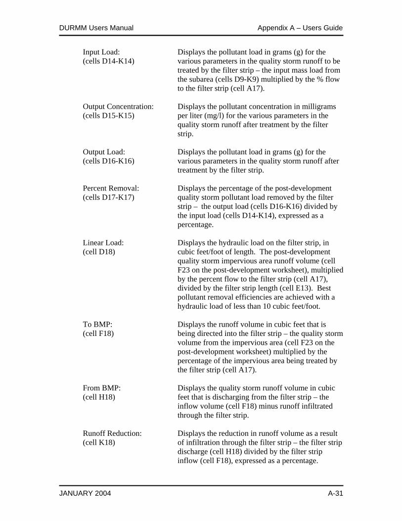
DURMM Users Manual Appendix A – Users Guide
JANUARY 2004 A-31
Input Load: Displays the pollutant load in grams (g) for the (cells D14-K14) various parameters in the quality storm runoff to be treated by the filter strip – the input mass load from the subarea (cells D9-K9) multiplied by the % flow to the filter strip (cell A17). Output Concentration: Displays the pollutant concentration in milligrams (cells D15-K15) per liter (mg/l) for the various parameters in the quality storm runoff after treatment by the filter strip. Output Load: Displays the pollutant load in grams (g) for the (cells D16-K16) various parameters in the quality storm runoff after treatment by the filter strip. Percent Removal: Displays the percentage of the post-development (cells D17-K17) quality storm pollutant load removed by the filter strip – the output load (cells D16-K16) divided by the input load (cells D14-K14), expressed as a percentage. Linear Load: Displays the hydraulic load on the filter strip, in (cell D18) cubic feet/foot of length. The post-development quality storm impervious area runoff volume (cell F23 on the post-development worksheet), multiplied by the percent flow to the filter strip (cell A17), divided by the filter strip length (cell E13). Best pollutant removal efficiencies are achieved with a hydraulic load of less than 10 cubic feet/foot. To BMP: Displays the runoff volume in cubic feet that is (cell F18) being directed into the filter strip – the quality storm volume from the impervious area (cell F23 on the post-development worksheet) multiplied by the percentage of the impervious area being treated by the filter strip (cell A17). From BMP: Displays the quality storm runoff volume in cubic (cell H18) feet that is discharging from the filter strip – the inflow volume (cell F18) minus runoff infiltrated through the filter strip. Runoff Reduction: Displays the reduction in runoff volume as a result (cell K18) of infiltration through the filter strip – the filter strip discharge (cell H18) divided by the filter strip inflow (cell F18), expressed as a percentage.
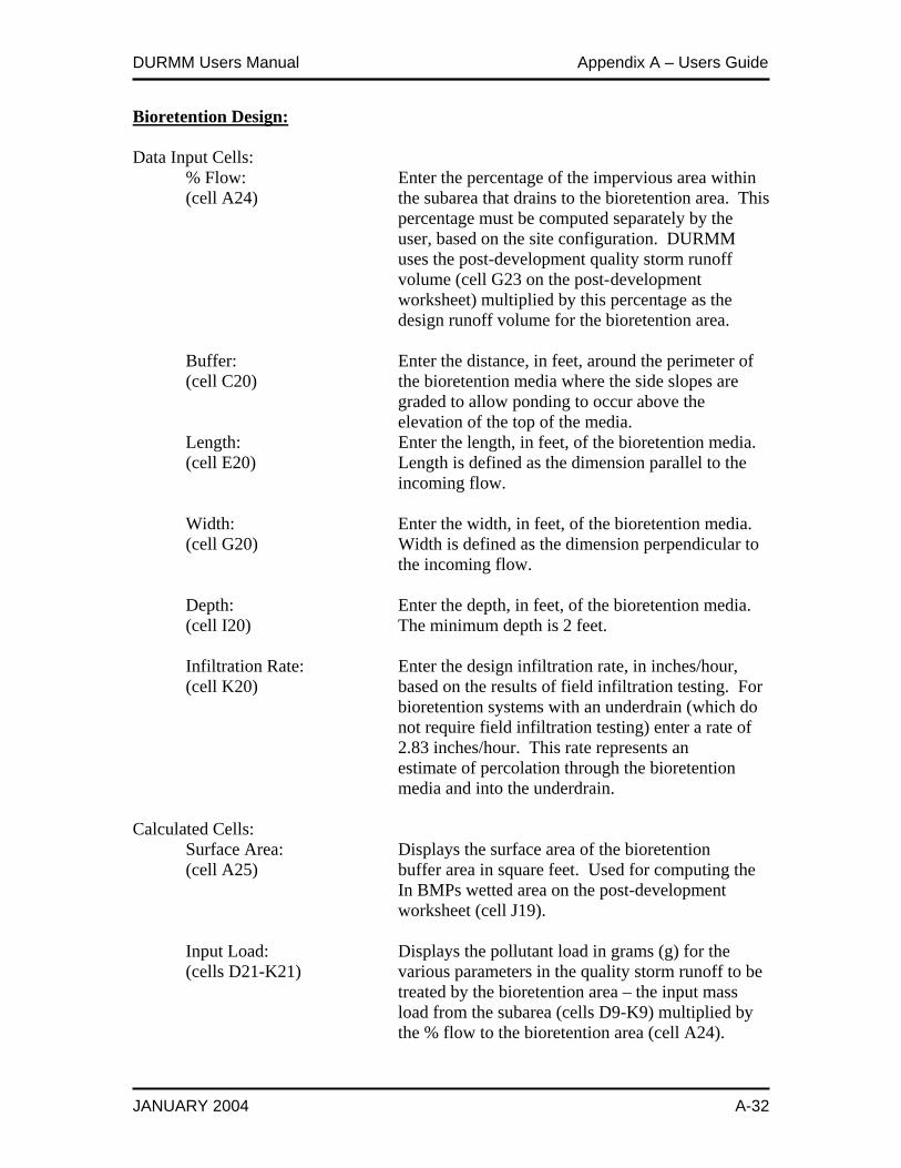
DURMM Users Manual Appendix A – Users Guide
JANUARY 2004 A-32
Bioretention Design: Data Input Cells: % Flow: Enter the percentage of the impervious area within (cell A24) the subarea that drains to the bioretention area. This percentage must be computed separately by the user, based on the site configuration. DURMM uses the post-development quality storm runoff volume (cell G23 on the post- development worksheet) multiplied by this percentage as the design runoff volume for the bioretention area. Buffer: Enter the distance, in feet, around the perimeter of (cell C20) the bioretention media where the side slopes are graded to allow ponding to occur above the elevation of the top of the media.
Length: Enter the length, in feet, of the bioretention media. (cell E20) Length is defined as the dimension parallel to the incoming flow. Width: Enter the width, in feet, of the bioretention media. (cell G20) Width is defined as the dimension perpendicular to the incoming flow. Depth: Enter the depth, in feet, of the bioretention media. (cell I20) The minimum depth is 2 feet. Infiltration Rate: Enter the design infiltration rate, in inches/hour, (cell K20) based on the results of field infiltration testing. For bioretention systems with an underdrain (which do not require field infiltration testing) enter a rate of 2.83 inches/hour. This rate represents an estimate of percolation through the bioretention media and into the underdrain.
Calculated Cells: Surface Area: Displays the surface area of the bioretention (cell A25) buffer area in square feet. Used for computing the In BMPs wetted area on the post-development worksheet (cell J19). Input Load: Displays the pollutant load in grams (g) for the (cells D21-K21) various parameters in the quality storm runoff to be treated by the bioretention area – the input mass load from the subarea (cells D9-K9) multiplied by the % flow to the bioretention area (cell A24).

DURMM Users Manual Appendix A – Users Guide
JANUARY 2004 A-33
Output Concentration: Displays the pollutant concentration in milligrams (cells D22-K22) per liter (mg/l) for the various parameters in the quality storm runoff after treatment by the bioretention area. Output Load: Displays the pollutant load in grams (g) for the (cells D23-K23) various parameters in the quality storm runoff after treatment by the bioretention area. Percent Removal: Displays the percentage of the post-development (cells D24-K24) quality storm pollutant load removed by the bioretention area – the output load (cells D23-K23) divided by the input load (cells D21-K21), expressed as a percentage. Hydraulic Load: Displays the hydraulic load on the bioretention (cell D25) area, in feet. The post-development quality storm runoff volume (cell G23 on the post-development worksheet), multiplied by the percent flow to the bioretention area (cell A24), divided by the bioretention length times width (cell E20 times cell G20). The maximum hydraulic load is 2.75 feet, which represents a maximum ponding depth of 1.5 feet plus a saturated depth of 1.25 feet in the bioretention media (2 feet media thickness adjusted for void ratio). To BMP: Displays the runoff volume in cubic feet that is (cell F25) being directed into the bioretention area – the quality storm runoff volume (cell G23 on the post-development worksheet) multiplied by the percent flow to the bioretention area (cell A24). From BMP: Displays the quality storm runoff volume in cubic (cell H25) feet that is discharging via surface flow from the bioretention area – the inflow volume (cell F25) minus runoff infiltrated through the bioretention media. Runoff Reduction: Displays the reduction in runoff volume as a result (cell K25) of infiltration through the bioretention media – the bioretention surface discharge volume (cell H25) divided by the inflow volume (cell F25), expressed as a percentage.

DURMM Users Manual Appendix A – Users Guide
JANUARY 2004 A-34
Bioswale Quality Design: Data Input Cells: % Flow: Enter the percentage of the impervious area within (cell A32) the subarea that drains to the bioswale. This percentage must be computed separately by the user, based on the site configuration. DURMM uses the post-development quality storm volume (cell G23 on the post-development worksheet) multiplied by this percentage as the design runoff volume for the bioretention area.
CN: Enter the curve number representing the vegetative (cell C27) cover and hydrologic soil group at the bioswale location. Slope: Enter the longitudinal slope of the bioswale, in (cell C28) feet/foot. Length: Enter the length of the bioswale, in feet. (cell E27) Cover: Enter one of the following cover codes to represent (cell E28) the bioswale surface cover type (see cells M29- O33): 1 – Pavement 2 – Stone/unpaved 3 – Short grass 4 – Dense grass 5 – Thick brush The cover type is displayed in cells F28-G28. Sides:1: Enter the horizontal portion of the bioswale side (cell G27) slope ratio, expressed with the vertical portion equal to 1. Bottom: Enter the bioswale bottom width, in feet. (cell I27)
Calculated Cells: Swale OK?: Displays “OK” after swale computations have been (cell K27) completed. If this cell displays “####”, click on the “Swale” button to complete the bioswale design computations.

DURMM Users Manual Appendix A – Users Guide
JANUARY 2004 A-35
Velocity: Displays the flow velocity, in feet per second, in (cell I28) the bioswale for the quality storm event. Depth: Displays the flow depth, in feet, in the bioswale for (cell K28) the quality storm event. Surface Area: Displays the surface area of the bioswale, in square (cell A33) feet, assuming a 3 inch flow depth in the swale for the quality storm event. Input Load: Displays the pollutant load in grams (g) for the (cells D29-K29) various parameters in the quality storm runoff to be treated by the bioswale – the input mass load from the subarea (cells D9-K9) multiplied by the % flow to the bioswale (cell A32). Output Concentration: Displays the pollutant concentration in milligrams (cells D30-K30) per liter (mg/l) for the various parameters in the quality storm runoff after treatment by the bioswale. Output Load: Displays the pollutant load in grams (g) for the (cells D31-K31) various parameters in the quality storm runoff after treatment by the bioswale. Percent Removal: Displays the percentage of the post-development (cells D32-K32) quality storm pollutant load removed by the bioswale – the output load (cells D31-K31) divided by the input load (cells D29-K29), expressed as a percentage. Residence Time: Displays the residence time, in minutes, in the (cell D33) bioswale for the quality storm event. To BMP: Displays the runoff volume in cubic feet that is (cell F33) being directed into the bioswale – the quality storm runoff volume (cell G23 on the post-development worksheet) multiplied by the percent flow to the bioretention area (cell A32). From BMP: Displays the quality storm runoff volume in cubic (cell H33) feet that is discharging from the bioswale – the inflow volume (cell F33) minus runoff infiltrated through the bioswale.

DURMM Users Manual Appendix A – Users Guide
JANUARY 2004 A-36
Runoff Reduction: Displays the reduction in runoff volume as a result (cell K33) of infiltration through the bioswale – the bioswale discharge volume (cell H33) divided by the inflow volume (cell F33), expressed as a percentage. Bioswale Capacity and Stability Check: Calculated Cells: Velocity: Displays the flow velocity, in feet per second, in the (cell B35) bioswale in the conveyance (10-year) storm event. Flow velocity should be less than 5 feet per second to ensure stability against erosion. OK/Dams prompt: Displays “OK” if the bioswale velocity is less than (cell B36) 5 feet per second in the conveyance (10-year) storm event. Displays “Dams” when the velocity is greater than or equal to 5 feet per second, as a prompt for the designer to consider the use of check dams in the swale to reduce the velocity, or redesign the swale. Capacity Depth: Displays the flow depth, in feet, in the bioswale for (cell B39) the conveyance (10-year) storm event. The designer should ensure that the swale grades on the plans accommodate at least this design depth, plus freeboard. Bioswale Volumes and Check Dam Design: Data Input Cells: Number of dams: Input the desired number of check dams to be (cell D35) placed equally spaced along the length of the bioswale. The check dam height will be computed based on the bioswale slope and the check dam spacing.
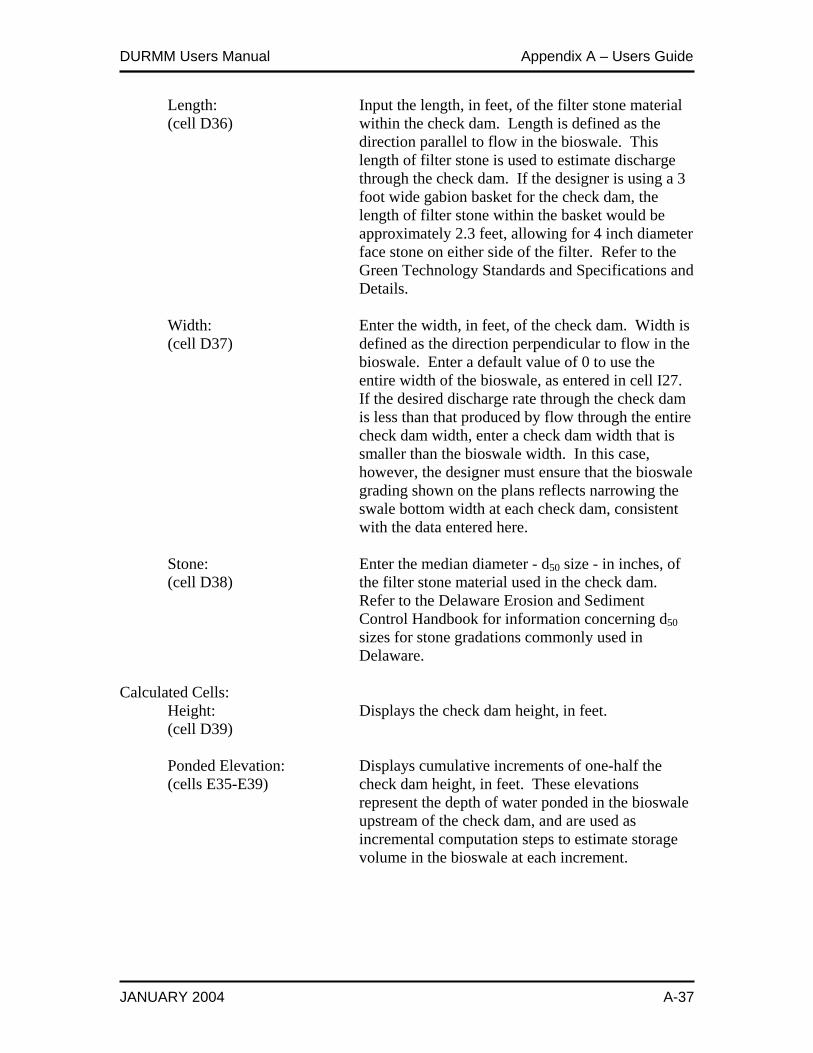
DURMM Users Manual Appendix A – Users Guide
JANUARY 2004 A-37
Length: Input the length, in feet, of the filter stone material (cell D36) within the check dam. Length is defined as the direction parallel to flow in the bioswale. This length of filter stone is used to estimate discharge through the check dam. If the designer is using a 3 foot wide gabion basket for the check dam, the length of filter stone within the basket would be approximately 2.3 feet, allowing for 4 inch diameter face stone on either side of the filter. Refer to the Green Technology Standards and Specifications and Details. Width: Enter the width, in feet, of the check dam. Width is (cell D37) defined as the direction perpendicular to flow in the bioswale. Enter a default value of 0 to use the entire width of the bioswale, as entered in cell I27. If the desired discharge rate through the check dam is less than that produced by flow through the entire check dam width, enter a check dam width that is smaller than the bioswale width. In this case, however, the designer must ensure that the bioswale grading shown on the plans reflects narrowing the swale bottom width at each check dam, consistent with the data entered here. Stone: Enter the median diameter - d50 size - in inches, of (cell D38) the filter stone material used in the check dam. Refer to the Delaware Erosion and Sediment Control Handbook for information concerning d50 sizes for stone gradations commonly used in Delaware. Calculated Cells: Height: Displays the check dam height, in feet. (cell D39) Ponded Elevation: Displays cumulative increments of one-half the (cells E35-E39) check dam height, in feet. These elevations represent the depth of water ponded in the bioswale upstream of the check dam, and are used as incremental computation steps to estimate storage volume in the bioswale at each increment.
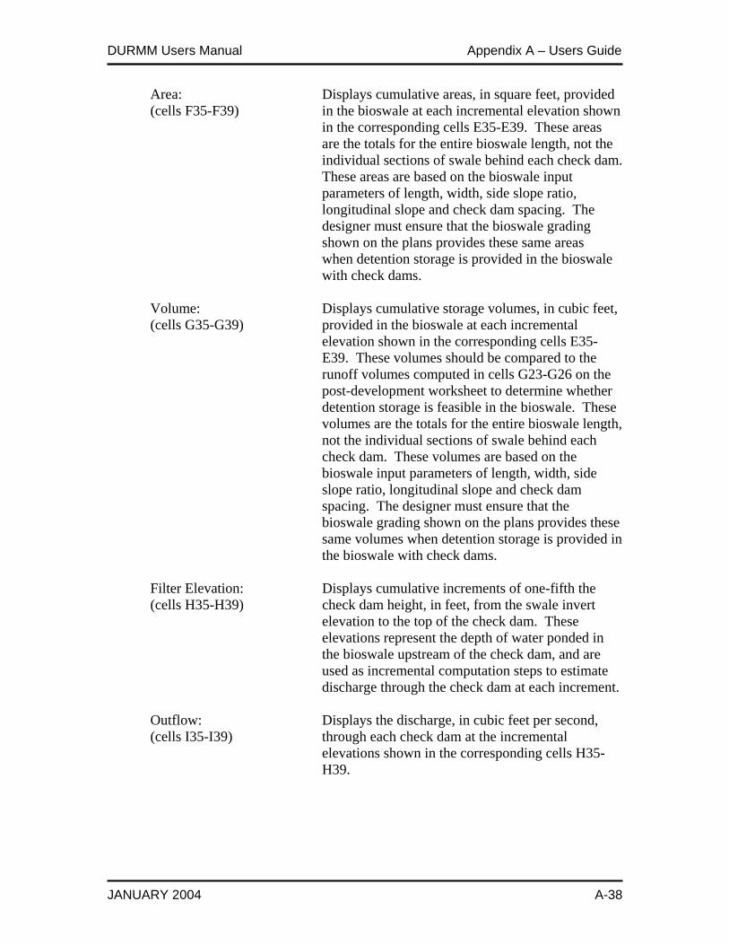
DURMM Users Manual Appendix A – Users Guide
JANUARY 2004 A-38
Area: Displays cumulative areas, in square feet, provided (cells F35-F39) in the bioswale at each incremental elevation shown in the corresponding cells E35-E39. These areas are the totals for the entire bioswale length, not the individual sections of swale behind each check dam. These areas are based on the bioswale input parameters of length, width, side slope ratio, longitudinal slope and check dam spacing. The designer must ensure that the bioswale grading shown on the plans provides these same areas when detention storage is provided in the bioswale with check dams. Volume: Displays cumulative storage volumes, in cubic feet, (cells G35-G39) provided in the bioswale at each incremental elevation shown in the corresponding cells E35- E39. These volumes should be compared to the runoff volumes computed in cells G23-G26 on the post-development worksheet to determine whether detention storage is feasible in the bioswale. These volumes are the totals for the entire bioswale length, not the individual sections of swale behind each check dam. These volumes are based on the bioswale input parameters of length, width, side slope ratio, longitudinal slope and check dam spacing. The designer must ensure that the bioswale grading shown on the plans provides these same volumes when detention storage is provided in the bioswale with check dams. Filter Elevation: Displays cumulative increments of one-fifth the (cells H35-H39) check dam height, in feet, from the swale invert elevation to the top of the check dam. These elevations represent the depth of water ponded in the bioswale upstream of the check dam, and are used as incremental computation steps to estimate discharge through the check dam at each increment. Outflow: Displays the discharge, in cubic feet per second, (cells I35-I39) through each check dam at the incremental elevations shown in the corresponding cells H35- H39.
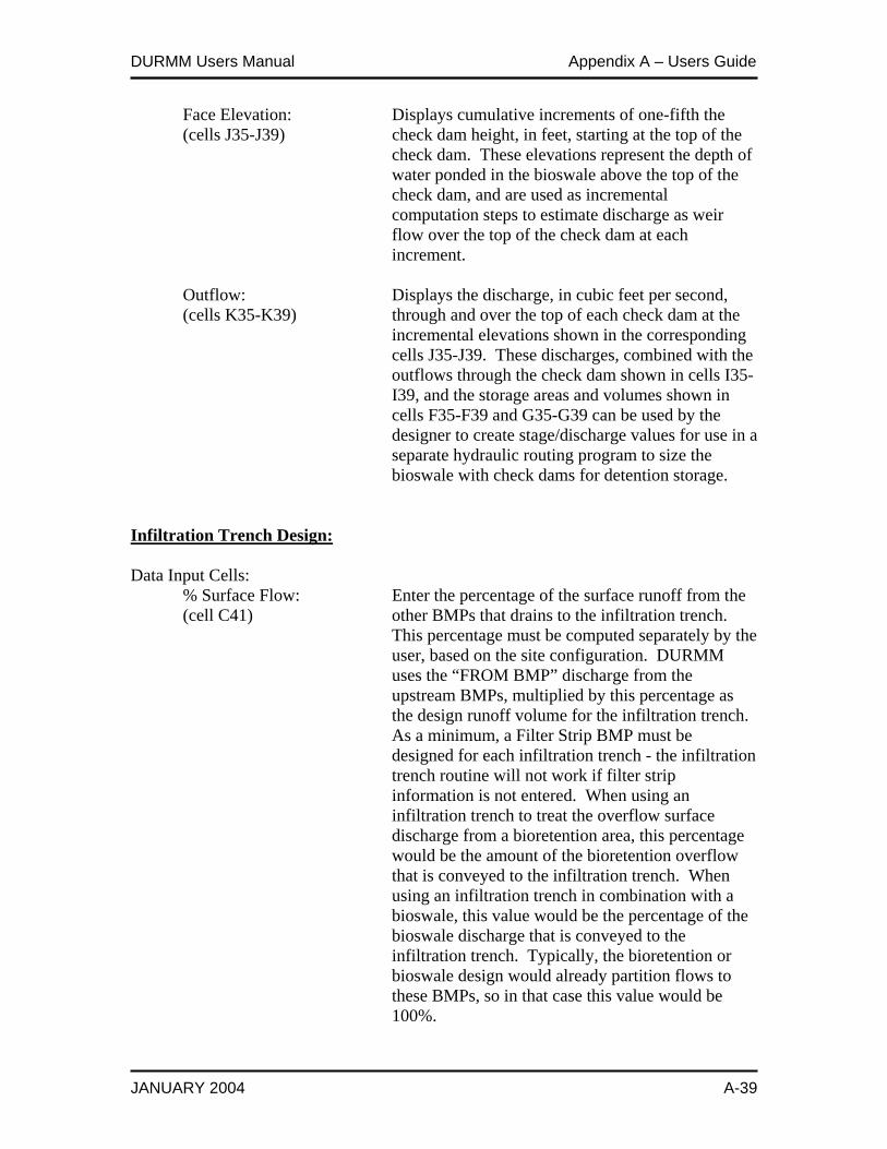
DURMM Users Manual Appendix A – Users Guide
JANUARY 2004 A-39
Face Elevation: Displays cumulative increments of one-fifth the (cells J35-J39) check dam height, in feet, starting at the top of the check dam. These elevations represent the depth of water ponded in the bioswale above the top of the check dam, and are used as incremental computation steps to estimate discharge as weir flow over the top of the check dam at each increment. Outflow: Displays the discharge, in cubic feet per second, (cells K35-K39) through and over the top of each check dam at the incremental elevations shown in the corresponding cells J35-J39. These discharges, combined with the outflows through the check dam shown in cells I35- I39, and the storage areas and volumes shown in cells F35-F39 and G35-G39 can be used by the designer to create stage/discharge values for use in a separate hydraulic routing program to size the bioswale with check dams for detention storage. Infiltration Trench Design: Data Input Cells: % Surface Flow: Enter the percentage of the surface runoff from the (cell C41) other BMPs that drains to the infiltration trench. This percentage must be computed separately by the user, based on the site configuration. DURMM uses the “FROM BMP” discharge from the upstream BMPs, multiplied by this percentage as the design runoff volume for the infiltration trench. As a minimum, a Filter Strip BMP must be designed for each infiltration trench - the infiltration trench routine will not work if filter strip information is not entered. When using an infiltration trench to treat the overflow surface discharge from a bioretention area, this percentage would be the amount of the bioretention overflow that is conveyed to the infiltration trench. When using an infiltration trench in combination with a bioswale, this value would be the percentage of the bioswale discharge that is conveyed to the infiltration trench. Typically, the bioretention or bioswale design would already partition flows to these BMPs, so in that case this value would be 100%.
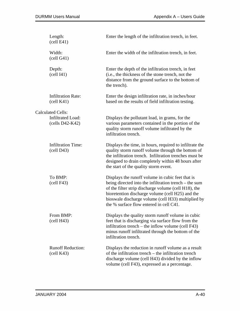
DURMM Users Manual Appendix A – Users Guide
JANUARY 2004 A-40
Length: Enter the length of the infiltration trench, in feet. (cell E41) Width: Enter the width of the infiltration trench, in feet. (cell G41) Depth: Enter the depth of the infiltration trench, in feet (cell I41) (i.e., the thickness of the stone trench, not the distance from the ground surface to the bottom of the trench). Infiltration Rate: Enter the design infiltration rate, in inches/hour (cell K41) based on the results of field infiltration testing. Calculated Cells: Infiltrated Load: Displays the pollutant load, in grams, for the (cells D42-K42) various parameters contained in the portion of the quality storm runoff volume infiltrated by the infiltration trench. Infiltration Time: Displays the time, in hours, required to infiltrate the (cell D43) quality storm runoff volume through the bottom of the infiltration trench. Infiltration trenches must be designed to drain completely within 48 hours after the start of the quality storm event. To BMP: Displays the runoff volume in cubic feet that is (cell F43) being directed into the infiltration trench – the sum of the filter strip discharge volume (cell H18), the bioretention discharge volume (cell H25) and the bioswale discharge volume (cell H33) multiplied by the % surface flow entered in cell C41. From BMP: Displays the quality storm runoff volume in cubic (cell H43) feet that is discharging via surface flow from the infiltration trench – the inflow volume (cell F43) minus runoff infiltrated through the bottom of the infiltration trench. Runoff Reduction: Displays the reduction in runoff volume as a result (cell K43) of the infiltration trench – the infiltration trench discharge volume (cell H43) divided by the inflow volume (cell F43), expressed as a percentage.
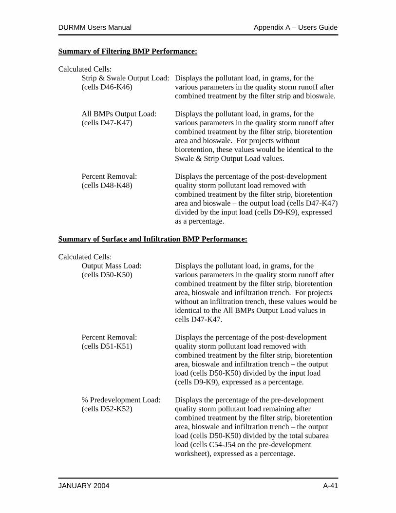
DURMM Users Manual Appendix A – Users Guide
JANUARY 2004 A-41
Summary of Filtering BMP Performance: Calculated Cells: Strip & Swale Output Load: Displays the pollutant load, in grams, for the (cells D46-K46) various parameters in the quality storm runoff after combined treatment by the filter strip and bioswale. All BMPs Output Load: Displays the pollutant load, in grams, for the (cells D47-K47) various parameters in the quality storm runoff after combined treatment by the filter strip, bioretention area and bioswale. For projects without bioretention, these values would be identical to the Swale & Strip Output Load values. Percent Removal: Displays the percentage of the post-development (cells D48-K48) quality storm pollutant load removed with combined treatment by the filter strip, bioretention area and bioswale – the output load (cells D47-K47) divided by the input load (cells D9-K9), expressed as a percentage. Summary of Surface and Infiltration BMP Performance: Calculated Cells: Output Mass Load: Displays the pollutant load, in grams, for the (cells D50-K50) various parameters in the quality storm runoff after combined treatment by the filter strip, bioretention area, bioswale and infiltration trench. For projects without an infiltration trench, these values would be identical to the All BMPs Output Load values in cells D47-K47. Percent Removal: Displays the percentage of the post-development (cells D51-K51) quality storm pollutant load removed with combined treatment by the filter strip, bioretention area, bioswale and infiltration trench – the output load (cells D50-K50) divided by the input load (cells D9-K9), expressed as a percentage. % Predevelopment Load: Displays the percentage of the pre-development (cells D52-K52) quality storm pollutant load remaining after combined treatment by the filter strip, bioretention area, bioswale and infiltration trench – the output load (cells D50-K50) divided by the total subarea load (cells C54-J54 on the pre-development worksheet), expressed as a percentage.

DURMM Users Manual Appendix A – Users Guide
JANUARY 2004 A-42
This page left intentionally blank.

DURMM Users Manual Appendix B – Step by Step Guide
JANUARY 2004
Appendix B
Step by Step Guide

DURMM Users Manual Appendix B – Step by Step Guide
JANUARY 2004
This page left intentionally blank.
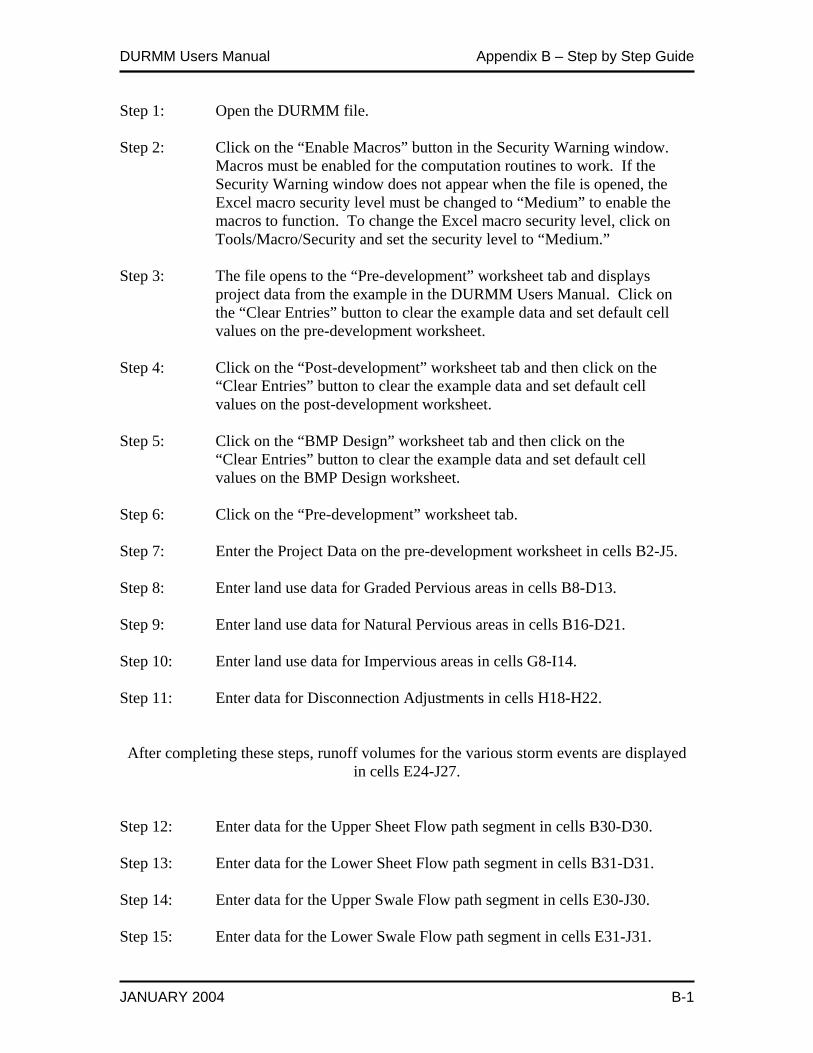
DURMM Users Manual Appendix B – Step by Step Guide
JANUARY 2004 B-1
Step 1: Open the DURMM file. Step 2: Click on the “Enable Macros” button in the Security Warning window. Macros must be enabled for the computation routines to work. If the Security Warning window does not appear when the file is opened, the Excel macro security level must be changed to “Medium” to enable the macros to function. To change the Excel macro security level, click on Tools/Macro/Security and set the security level to “Medium.” Step 3: The file opens to the “Pre-development” worksheet tab and displays project data from the example in the DURMM Users Manual. Click on the “Clear Entries” button to clear the example data and set default cell values on the pre-development worksheet. Step 4: Click on the “Post-development” worksheet tab and then click on the “Clear Entries” button to clear the example data and set default cell values on the post-development worksheet. Step 5: Click on the “BMP Design” worksheet tab and then click on the “Clear Entries” button to clear the example data and set default cell values on the BMP Design worksheet. Step 6: Click on the “Pre-development” worksheet tab. Step 7: Enter the Project Data on the pre-development worksheet in cells B2-J5. Step 8: Enter land use data for Graded Pervious areas in cells B8-D13. Step 9: Enter land use data for Natural Pervious areas in cells B16-D21. Step 10: Enter land use data for Impervious areas in cells G8-I14. Step 11: Enter data for Disconnection Adjustments in cells H18-H22.
After completing these steps, runoff volumes for the various storm events are displayed
in cells E24-J27. Step 12: Enter data for the Upper Sheet Flow path segment in cells B30-D30. Step 13: Enter data for the Lower Sheet Flow path segment in cells B31-D31. Step 14: Enter data for the Upper Swale Flow path segment in cells E30-J30. Step 15: Enter data for the Lower Swale Flow path segment in cells E31-J31.
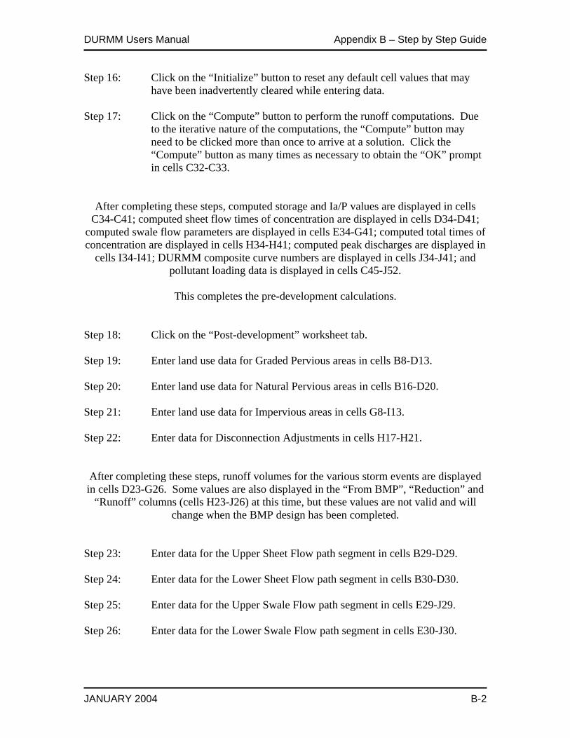
DURMM Users Manual Appendix B – Step by Step Guide
JANUARY 2004 B-2
Step 16: Click on the “Initialize” button to reset any default cell values that may have been inadvertently cleared while entering data. Step 17: Click on the “Compute” button to perform the runoff computations. Due to the iterative nature of the computations, the “Compute” button may need to be clicked more than once to arrive at a solution. Click the “Compute” button as many times as necessary to obtain the “OK” prompt in cells C32-C33.
After completing these steps, computed storage and Ia/P values are displayed in cells C34-C41; computed sheet flow times of concentration are displayed in cells D34-D41;
computed swale flow parameters are displayed in cells E34-G41; computed total times of concentration are displayed in cells H34-H41; computed peak discharges are displayed in
cells I34-I41; DURMM composite curve numbers are displayed in cells J34-J41; and pollutant loading data is displayed in cells C45-J52.
This completes the pre-development calculations.
Step 18: Click on the “Post-development” worksheet tab. Step 19: Enter land use data for Graded Pervious areas in cells B8-D13. Step 20: Enter land use data for Natural Pervious areas in cells B16-D20. Step 21: Enter land use data for Impervious areas in cells G8-I13. Step 22: Enter data for Disconnection Adjustments in cells H17-H21.
After completing these steps, runoff volumes for the various storm events are displayed in cells D23-G26. Some values are also displayed in the “From BMP”, “Reduction” and
“Runoff” columns (cells H23-J26) at this time, but these values are not valid and will change when the BMP design has been completed.
Step 23: Enter data for the Upper Sheet Flow path segment in cells B29-D29. Step 24: Enter data for the Lower Sheet Flow path segment in cells B30-D30. Step 25: Enter data for the Upper Swale Flow path segment in cells E29-J29. Step 26: Enter data for the Lower Swale Flow path segment in cells E30-J30.
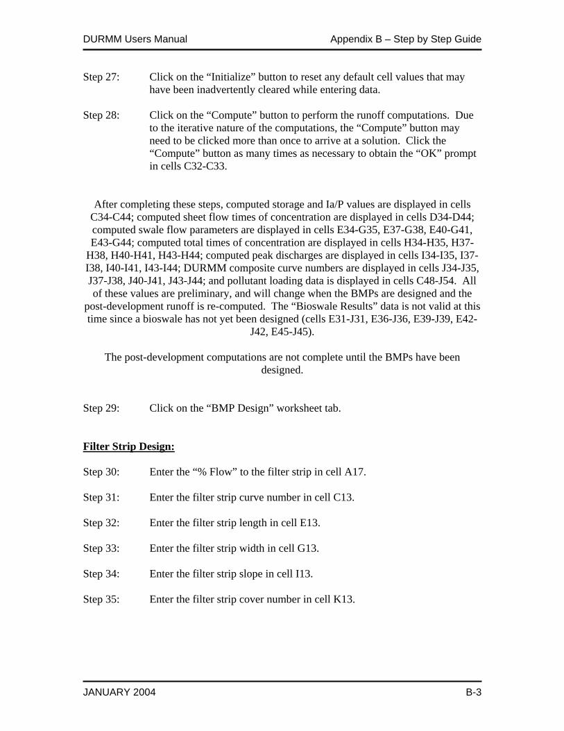
DURMM Users Manual Appendix B – Step by Step Guide
JANUARY 2004 B-3
Step 27: Click on the “Initialize” button to reset any default cell values that may have been inadvertently cleared while entering data. Step 28: Click on the “Compute” button to perform the runoff computations. Due to the iterative nature of the computations, the “Compute” button may need to be clicked more than once to arrive at a solution. Click the “Compute” button as many times as necessary to obtain the “OK” prompt in cells C32-C33.
After completing these steps, computed storage and Ia/P values are displayed in cells C34-C44; computed sheet flow times of concentration are displayed in cells D34-D44; computed swale flow parameters are displayed in cells E34-G35, E37-G38, E40-G41, E43-G44; computed total times of concentration are displayed in cells H34-H35, H37-
H38, H40-H41, H43-H44; computed peak discharges are displayed in cells I34-I35, I37-I38, I40-I41, I43-I44; DURMM composite curve numbers are displayed in cells J34-J35, J37-J38, J40-J41, J43-J44; and pollutant loading data is displayed in cells C48-J54. All of these values are preliminary, and will change when the BMPs are designed and the
post-development runoff is re-computed. The “Bioswale Results” data is not valid at this time since a bioswale has not yet been designed (cells E31-J31, E36-J36, E39-J39, E42-
J42, E45-J45).
The post-development computations are not complete until the BMPs have been designed.
Step 29: Click on the “BMP Design” worksheet tab. Filter Strip Design:
Step 30: Enter the “% Flow” to the filter strip in cell A17.
Step 31: Enter the filter strip curve number in cell C13.
Step 32: Enter the filter strip length in cell E13.
Step 33: Enter the filter strip width in cell G13.
Step 34: Enter the filter strip slope in cell I13.
Step 35: Enter the filter strip cover number in cell K13.

DURMM Users Manual Appendix B – Step by Step Guide
JANUARY 2004 B-4
Step 36: Check the “Area OK” and “Load OK” prompts in cells I12 and K12. If the “Area OK” prompt displays “#####” instead of “OK”, then the total Graded Pervious area entered on the post- development sheet is smaller than the filter strip area. If the “Load OK” prompt displays “#####” instead of “OK” either the filter strip area is too small or the “% flow” exceeds 100%. Repeat steps 30-35 with different data values until both these prompts display “OK.”
At this point the filter strip design is complete; but the post-development runoff must be re-computed to include the effects of the filter strip.
Step 37: Click the “Post-development” worksheet tab. Step 38: Click on the “Initialize” button to reset any default cell values that may have been inadvertently cleared while entering data. Step 39: Click on the “Compute” button to revise the runoff computations to include the filter strip effects. Due to the iterative nature of the computations, the “Compute” button may need to be clicked more than once to arrive at a solution. Click the “Compute” button as many times as necessary to obtain the “OK” prompt in cells C32- C33.
This completes the post-development calculations for a filter strip design. Bioretention Design:
Complete steps 30-36 if a filter strip is being used as pre-treatment for the bioretention area, otherwise skip steps 30-39.
Step 40: Enter the “% Flow” to the bioretention area in cell A24. Step 41: Enter the bioretention area buffer width in cell C20. Step 42: Enter the bioretention area length in cell E20. Step 43: Enter the bioretention area width in cell G20. Step 44: Enter the thickness of the bioretention planting soil media in cell I20.

DURMM Users Manual Appendix B – Step by Step Guide
JANUARY 2004 B-5
Step 45: Enter the bioretention area infiltration rate in cell K20. Step 46: Check the “Bio OK”, “Area OK” and “Load OK” prompts in cells G12, I12 and K12. If the “Bio OK” prompt displays “#####” instead of “OK” then the hydraulic load on the bioretention area exceeds 2.75 feet (see cell D25) – either make the bioretention area larger or reduce the % flow. If the “Area OK” prompt displays “#####” instead of “OK”, then the total Graded Pervious area entered on the post-development sheet is smaller than the bioretention area. If the “Load OK” prompt displays “#####” instead of “OK” the “% flow” exceeds 100%. Repeat steps 40-45 with different data values until all these prompts display “OK.”
At this point the bioretention design is complete; but the post-development runoff must be re-computed to include the effects of bioretention.
Step 47: Click the “Post-development” worksheet tab. Step 48: Click on the “Initialize” button to reset any default cell values that may have been inadvertently cleared while entering data. Step 49: Click on the “Compute” button to revise the runoff computations to include the bioretention area effects. Due to the iterative nature of the computations, the “Compute” button may need to be clicked more than once to arrive at a solution. Click the “Compute” button as many times as necessary to obtain the “OK” prompt in cells C32- C33.
This completes the post-development calculations for a bioretention design. Biofiltration Swale Design:
Skip steps 30-49. Step 50: Enter the “% Flow” to the bioswale in cell A32. Step 51: Enter the bioswale curve number in cell C27. Step 52: Enter the bioswale slope in cell C28. Step 53: Enter the bioswale length in cell E27.
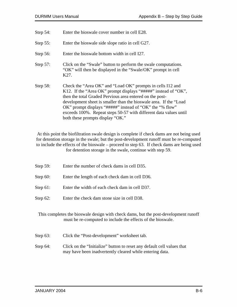
DURMM Users Manual Appendix B – Step by Step Guide
JANUARY 2004 B-6
Step 54: Enter the bioswale cover number in cell E28. Step 55: Enter the bioswale side slope ratio in cell G27. Step 56: Enter the bioswale bottom width in cell I27. Step 57: Click on the “Swale” button to perform the swale computations. “OK” will then be displayed in the “Swale/OK” prompt in cell K27. Step 58: Check the “Area OK” and “Load OK” prompts in cells I12 and K12. If the “Area OK” prompt displays “#####” instead of “OK”, then the total Graded Pervious area entered on the post- development sheet is smaller than the bioswale area. If the “Load OK” prompt displays “#####” instead of “OK” the “% flow” exceeds 100%. Repeat steps 50-57 with different data values until both these prompts display “OK.” At this point the biofiltration swale design is complete if check dams are not being used for detention storage in the swale; but the post-development runoff must be re-computed to include the effects of the bioswale – proceed to step 63. If check dams are being used
for detention storage in the swale, continue with step 59.
Step 59: Enter the number of check dams in cell D35. Step 60: Enter the length of each check dam in cell D36. Step 61: Enter the width of each check dam in cell D37. Step 62: Enter the check dam stone size in cell D38.
This completes the bioswale design with check dams, but the post-development runoff must be re-computed to include the effects of the bioswale.
Step 63: Click the “Post-development” worksheet tab. Step 64: Click on the “Initialize” button to reset any default cell values that may have been inadvertently cleared while entering data.
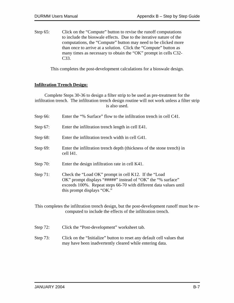
DURMM Users Manual Appendix B – Step by Step Guide
JANUARY 2004 B-7
Step 65: Click on the “Compute” button to revise the runoff computations to include the bioswale effects. Due to the iterative nature of the computations, the “Compute” button may need to be clicked more than once to arrive at a solution. Click the “Compute” button as many times as necessary to obtain the “OK” prompt in cells C32- C33.
This completes the post-development calculations for a bioswale design.
Infiltration Trench Design:
Complete Steps 30-36 to design a filter strip to be used as pre-treatment for the infiltration trench. The infiltration trench design routine will not work unless a filter strip
is also used. Step 66: Enter the “% Surface” flow to the infiltration trench in cell C41. Step 67: Enter the infiltration trench length in cell E41. Step 68: Enter the infiltration trench width in cell G41. Step 69: Enter the infiltration trench depth (thickness of the stone trench) in cell I41. Step 70: Enter the design infiltration rate in cell K41. Step 71: Check the “Load OK” prompt in cell K12. If the “Load OK” prompt displays “#####” instead of “OK” the “% surface” exceeds 100%. Repeat steps 66-70 with different data values until this prompt displays “OK.”
This completes the infiltration trench design, but the post-development runoff must be re-computed to include the effects of the infiltration trench.
Step 72: Click the “Post-development” worksheet tab. Step 73: Click on the “Initialize” button to reset any default cell values that may have been inadvertently cleared while entering data.

DURMM Users Manual Appendix B – Step by Step Guide
JANUARY 2004 B-8
Step 74: Click on the “Compute” button to revise the runoff computations to include the infiltration trench effects. Due to the iterative nature of the computations, the “Compute” button may need to be clicked more than once to arrive at a solution. Click the “Compute” button as many times as necessary to obtain the “OK” prompt in cells C32- C33.
This completes the post-development calculations for an infiltration trench design.