DTN-FLOW: Inter-Landmark Data Flow forHigh-Throughput Routing in DTNs

Kang Chen and Haiying ShenDepartment of Electrical and Computer Engineering

Clemson University, Clemson, SC 29631Email: {kangc, shenh}@clemson.edu

Abstract—In this paper, we focus on the efficient routing ofdata among different areas in Delay Tolerant Networks (DTNs).In current algorithms, packets are forwarded gradually throughnodes with higher probability of visiting the destination nodeor area. However, the number of such nodes usually is limited,leading to insufficient throughput performance. To solve thisproblem, we propose an inter-landmark data routing algorithm,namely DTN-FLOW. It selects popular places that nodes visitfrequently as landmarks and divides the entire DTN area intosub-areas represented by landmarks. Nodes transiting betweenlandmarks relay packets among landmarks, even though theyrarely visit the destinations of these packets. Specifically, thenumber of node transits between two landmarks is measured torepresent the forwarding capacity between them, based on whichrouting tables are built on each landmark to guide packet routing.Each node predicts its transits based on its previous landmarkvisiting records using the order-k Markov predictor. In a packetrouting, a landmark determines the next hop landmark basedon its routing table, and forwards the packet to the node withthe highest probability of transiting to the selected landmark.Thus, DTN-FLOW fully utilizes all node movements to routepackets along landmark paths to their destinations. We analyzedtwo real DTN traces to support the design of DTN-FLOW.We also deployed a small DTN-FLOW system in our campusfor performance evaluation. This deployment and trace-drivensimulation demonstrate the high efficiency of DTN-FLOW incomparison with state-of-the-art DTN routing algorithms.

I. INTRODUCTION

Delay tolerant networks (DTNs) are featured by intermittentconnection and frequent network partition. Thus, DTN routingis usually realized in a carry-store-forward manner [1], whichmakes it possible to develop useful applications over suchchallenging environments. Among many applications, we areparticularly interested in those that exchange data amongor collect data from different areas because DTNs usuallyexist in areas without infrastructure networks and thereby aregood mediums to realize data communication among theseareas. For example, researchers have proposed to provide datacommunications (i.e., Internet access) to remote and ruralareas [2] by relying on people or vehicles moving amongrural villages and cities to carry and forward data. The conceptof DTN has also been applied in animal tracking [3], whichcollects logged data from the digital collars attached to zebrasin Kenya without infrastructure network, and in environmentalmonitoring, where data is collected by sensors deployed onanimals in mountain areas.

Since these applications tend to transmit high volumes ofdata (i.e., Internet data, collected logs and monitoring data), a

A1 A2 A3

A4 A5 A6

A7 A8 A9

N1N1N2

N2

N3

N3

A1 A2 A3

A4 A5 A6

A7 A8 A9

(a) Previous Methods (b) DTN‐FLOW

Nodemovement

Packet forwarding

All node 

movements

L1 L2

L5

L8 L9

Fig. 1: Comparison between previous methods and DTN-FLOW.

key hurdle in developing these applications is efficient datarouting with high throughput. This challenge is non-trivialdue to the DTN features mentioned previously. Epidemicrouting [4], in which each node forwards its packets to all ofits neighbors, can route packets to their destinations quickly.However, its broadcast nature consumes high energy andstorage resource, which makes it unsuitable for the resource-limited DTNs [5]. Other DTN routing algorithms can generallybe classified into three groups: probabilistic routing [6]–[9],social network based routing [10]–[15] and location basedrouting [16]–[21]. They exploit either past encounter records,social network properties or past moving paths to deduce anode’s probability of reaching a certain node or area, andforward packets to nodes with higher probability than currentpacket holder. Figure 1(a) illustrates the routing process inprevious routing algorithms. A packet is generated in area A1for area A9. It is first carried by node N1 and then is forwardedto N2 in area A3 since N2 visits A9 more frequently. Later,similarly, the packet is forwarded to N3, which finally carriesthe packet to area A9. Since the number of nodes withhigh probability of visiting the destination usually is limited,by only relying on such nodes, previous routing algorithmsfail to fully utilize all node movements, leading to degradedefficiency and overall throughput. For example, even if thereare many node moving between A2 and A5, they are notutilized to forward the packet.

To deal with this problem, we propose an inter-landmarkdata flow routing algorithm, called DTN-FLOW, that fullyutilizes all node movements in DTNs. Figure 1(b) demon-strates DTN-FLOW. We assume that there is a popular placein each of the nine subareas in Figure 1(a). DTN-FLOW thendetermines landmarks from these popular places and adoptsthe same sub-area division as in Figure 1(a). Each sub-areais represented by one landmark. Each landmark is configuredwith a central station, which is an additional infrastructure with

high processing and storage capacity. Then, node movementcan be regarded as transits from one landmark to anotherlandmark. DTN-FLOW utilizes such transits to forward pack-ets one landmark by one landmark to reach their destinationareas. Nodes transiting between landmarks relay packets, eventhough they rarely or may even not visit the destinations of therelayed packets. We denote the landmark in each area in Figure1(b) by Li (i ∈ [1, 9]). For packets originated from area A1targeting area A9, they are forwarded along landmark L1, L2,L5, L8 to finally reach L9. Thus, DTN-FLOW fully utilizes thenode transiting between different pairs of landmarks for datatransmission (i.e., A2 and A5 in previous example), therebyincreasing the data flow throughput.

DTN-FLOW measures the amount of nodes moving fromone landmark, say Li, to another landmark, say Lj , to repre-sent the inter-landmark forwarding capacity from Li to Lj .This capacity indicates the data transfer capacity betweenlandmarks, hence is similar to the concept of “bandwidth” forphysical wired or wireless links. With the measured capacity,each landmark uses the distance-vector method [22] to buildits routing table that indicates the next hop landmark toreach each destination landmark. DTN-FLOW predicts nodetransits based on their previous landmark visiting recordsusing the order-k Markov predictor. Then, in packet routing,each landmark determines the next hop landmark based onits routing table, and forwards the packet to the node withthe highest probability of transiting to the selected landmark.Thus, DTN-FLOW fully utilizes the node transits to forwardpackets along landmark paths with the shortest latency toreach their destinations. The routing table is built with theDistance-vector method [22], in which each landmark informsall neighboring landmarks its routing table periodically. Uponreceiving a routing table, each landmark updates its routesto other landmarks with the next landmark hop leading to ashorter delay. In DTN-FLOW, the transmission of all infor-mation (i.e., routing tables and packets) among landmarks isconducted through mobile nodes.

Therefore, the proposed DTN-FLOW is suitable for ap-plications designed to transfer data among different areas inDTNs where distributed frequently visited locations can beidentified without extreme effort. Also, since the landmarkrequires a lightweight additional infrastructure, these locationsshould be able to provide continuous energy supply. Twocommon scenarios that satisfy above requirements are thethe data exchange between different buildings in campus andbetween different villages in rural areas. In both scenarios,mobile nodes (people) usually frequently visit different build-ings/villages that can provide energy supply easily.

We further analyzed two real DTN traces to confirm theshortcoming of the current routing algorithms and to supportthe design of DTN-FLOW. We also deployed a real DTN-FLOW system in our campus using 9 mobile phones forthe real-world performance evaluation. This real deploymentand extensive trace-driven simulation demonstrate the highthroughput and efficiency of DTN-FLOW in comparison withstate-of-the-art routing methods in DTNs.

The remainder of this paper is arranged as follows. Sec-tion II and III present related work and network model and realtrace analysis. Section IV introduces the detailed design of theDTN-FLOW system. In Section V, the performance of DTN-FLOW is evaluated through extensive trace-driven experimentsand a real deployment. Section VI concludes this paper withremarks on our future work.

II. RELATED WORK

A. Probabilistic Routing Methods

Probabilistic routing methods [6]–[9] use nodes’ past en-counter records to predict their future encounter probabilities,which is used to rank the suitability of a node to carry apacket. PROPHET [6] updates the encountering probabilitybetween two nodes when they meet and ages the probabilityover time. A packet is always forwarded to nodes withhigher probability of meeting its destination. MaxProp [7],RAPID [8], and MaxContribution [9] extend PROPHET byfurther specifying forwarding and storing priorities based onthe probability of successful delivery. Packets with higherpriorities are forwarded first, and high priority packets replacelow priory packets when a node’s storage is full.

B. Social Network Based Routing Methods

Considering that people carrying mobile devices usuallybelong to certain social relationships, social network basedrouting algorithms [10]–[15] exploits social network propertiesin DTNs for packet routing. MOPS [10] is a publish-subscribesystem. It groups frequently encountered nodes into a clusterfor efficient intra-community communication and selects nodeshaving frequent contacts with foreign communities for inter-community communication. BUBBLE [11] uses two layersof ranks: global and local. The global ranking is used toforward a packet to the destination community, and the localranking helps to find the destination within the community.The concept of two-layer routing is similar to the landmarkoverlay in DTN-FLOW. However, BUBBLE does not splitthe network into sub-areas but classifies nodes into differentcommunities. SimBet [12] adopts centrality and similarity torank the suitability of a node to carry a packet. It is based onthe concept that nodes having high centrality and similaritywith the destination node tend to meet it frequently. Theevent dissemination system in [13] is similar to MOPS. Itgroups well-connected nodes into communities and selectsnodes with the highest closeness centrality as brokers forinter-community dissemination. Costa et al. proposed a socialnetwork based publish-subscribe system [14]. It forwardsmessages to nodes that meet subscribers of the packet’s interestcategory frequently and have high connectivity with othernodes. HiBop [15] defines node context by jointly consideringvarious information, including personal interests, residenceand work, and forwards packets to the nodes that have frequentencounter records with the context of the destination.

C. Location Based Routing Methods

Location based routing methods [16]–[19], [21] use pre-vious geographical location visiting records to predict futuremovement and thereby decide the suitability of a node to carrya packet destined for a certain node or place. GeoDTN [16] en-codes historical geographical movement information in a vec-tor to predict the possibility of two nodes becoming neighbors.Then, packets are forwarded to nodes that are more likely tobe a neighbor of the destination node. DTFR [17] first decidesthe area that the destination node is expected to appear basedon its past location and mobility pattern, then routes the packetto the area, and finally spreads the packet across the areato reach the destination node. PGR [18] uses observed nodemobility pattern to predict nodes future movement to forwardpackets to a certain geographical destination. GeoOpps [19]exploits the navigation system to forward packets to certaingeographical destinations in vehicle networks. It calculates theminimal estimated time of delivery (METD) by consideringthe closest point of possible routes to the destination, andforwards packets to vehicles that lead to smaller METD.In MobyPoints [21], a node’s meeting probabilities with allpossible locations are encoded in vectors. Then, forwardingdecisions are made based on the similarity score between thevectors of relay node and destination node. LOUVRE [23] isa similar work with DTN-FLOW that it also builds landmarkson road intersections and uses the landmark overlay for routingin vehicle networks. However, LOUVRE focuses on vehicularnetworks that it relies on GPS and map to determine thecurrent landmark a node is connected to and the next landmarkthe node is moving toward. On the contrary, DTN-FLOW isdesigned for general DTNs, in which it is hard to know thenext landmark a node is moving to since nodes move freelyin the whole area. To solve this problem, DTN-FLOW adoptsa k-order Markov predictor and a novel method to handleprediction errors, as shown in Section IV-B and IV-D.

III. NETWORK MODEL AND TRACE ANALYSIS

A. Network Model

1) Network Description: We assume a DTN with mobilenodes denoted by Ni. Each node has limited storage space andcommunication range. We select landmarks, denoted by Li

(i = 1, 2, 3, · · · ,M ), from places that nodes visit frequently.Then, the entire DTN area is split into sub-areas based onlandmarks, each of which is represented by a landmark. Weconfigure a central station at each landmark, which has higherprocessing and storage capacity than mobile nodes and cancover its whole sub-area. As in other social network basedDTN routing algorithms [10]–[15], DTN-FLOW also assumesthe existence of social network structure in DTNs. Such socialstructures determine node movement, leading to re-appearingvisiting patterns to these landmarks.

A transit means a node disconnects from one landmarkand connects to another landmark in sequence. We denote thetransit link from landmark Li to landmark Lj as Tij . For atransit link, say Tij , we define the bandwidth as the average

number of nodes transiting from Li to Lj in a unit time (T ),denoted by Bij . For simplicity, we assume that each packethas a fixed size. Our work can be easily extended to packetswith various lengths by dividing a large packet into a numberof the same-size segments.

2) Packet Routing: In this paper, we focus on the routingof packets to a landmark/sub-area. Then, normal probabilisticrouting algorithms can be used to route packets to a specificlocation or node. DTN-FLOW can also employ the Cellular IPprotocol [24] to track node locations and forward the packetto the new landmark containing the node. We leave the detailof the two extensions as our future work.

3) Differences with Infrastructure Networks: ThoughDTN-FLOW presents similar overlay as the infrastructurenetwork (i.e., small sub-areas covered by landmarks), theyhave significant differences. Firstly, DTN-FLOW does notrequire landmarks to be inter-connected with fixed links.Rather, landmarks rely on the mobil nodes moving betweenthem to relay packets. Secondly, as we will show later, eachlandmark only functions as a special relay node in the packetrouting. Therefore, landmarks do not bring about server-clientstructure but keep the ad hoc nature of DTNs. Unlike basestations, landmarks are just static nodes in DTNs with higherprocessing capacity (e.g., a desktop).

This also means that the import of landmarks into DTNsonly needs to build some fixed nodes in the network, whichdoes not incur much extra effort. Though the landmark nodesrequire higher capacity in storage and energy compared tonormal mobile nodes, these requirements can be easily sat-isfied since landmarks can have continuous energy supply(i.e., solar or wind energy). It is easy to maintain landmarknodes since there is no global management responsibility orcontrol information stored on landmarks. When a landmarkmalfunctions, we can simply remove it and merge its area tothat of another landmark or replace it without network-levelre-configuration.

4) Purpose of Landmarks: In DTN-FLOW, landmarksfunction as “routers” in the network. Each landmark decidesthe neighboring landmark to forward its received packets.Neighboring landmarks are connected by “links” that takemobile nodes as the transfer media to carry packets. Withoutlandmarks, packets are relayed purely through mobile nodeswhen they meet with each other, which may suffer fromthe uncertainty of node mobility. Therefore, landmarks makethe DTN routing more structured (i.e., along landmarks) inthe network dynamism in DTNs. Moreover, as previouslymentioned, landmarks do not incur too much extra cost interms of installing and maintenance. In summary, the use oflandmarks in DTN-FLOW can better utilize node mobility inDTNs for efficient packet routing with a low extra cost.

B. Trace Analysis

In order to better understand how nodes transit amongdifferent landmarks in DTNs, we analyzed two real DTNtraces collected from two different scenarios: students oncampus and buses in the downtown area of a college town.

1) Empirical Datasets:Dartmouth Campus Trace (DART) [25]. DART recorded

the WLAN Access Point (AP) association with digital devicescarried by students in the Dartmouth campus between Nov.2, 2003 and Feb. 28, 2004. We preprocessed the trace to fitour investigation. We regarded each building as a landmarkand merged neighboring records referring to the same node(mobile device) and the same landmark. We also removedshort connections (< 200s) and nodes with fewer records(< 500). Finally, we obtained 320 nodes and 159 landmarks.

DieselNet AP Trace (DNET) [26]. DNET collected theAP association records from 34 buses in UMass Transit fromOct. 22, 2007 to Nov. 16, 2007 in Amherst, MA. Each buscarried a Diesel Brick that constantly scanned the surroundingarea for open AP connections, and a GPS to record its GPScoordinators. Since there are many APs in the outdoor testingenvironment, some of which are not from the experiment, weremoved APs that did not appear frequently (< 50) fromthe trace. We mapped APs that are within certain distance(< 1.5km) into one landmark. Similar to the processing ofthe DART trace, neighboring records refereing to the samenode (bus) and the same landmark were merged. Finally, weobtained 34 nodes and 18 landmarks.

The key characteristics of the two traces are summarized inTable I. We then measured the landmark visiting distributionand the transits of mobile nodes among landmarks.

TABLE I: Characteristics of mobility traces.

DART Campus (DART) DieselNet AP (DNET)# Nodes 320 34# Landmarks 159 18Duration 119 days 20 days# Transits 477803 25193# Transits per day 2401 1257

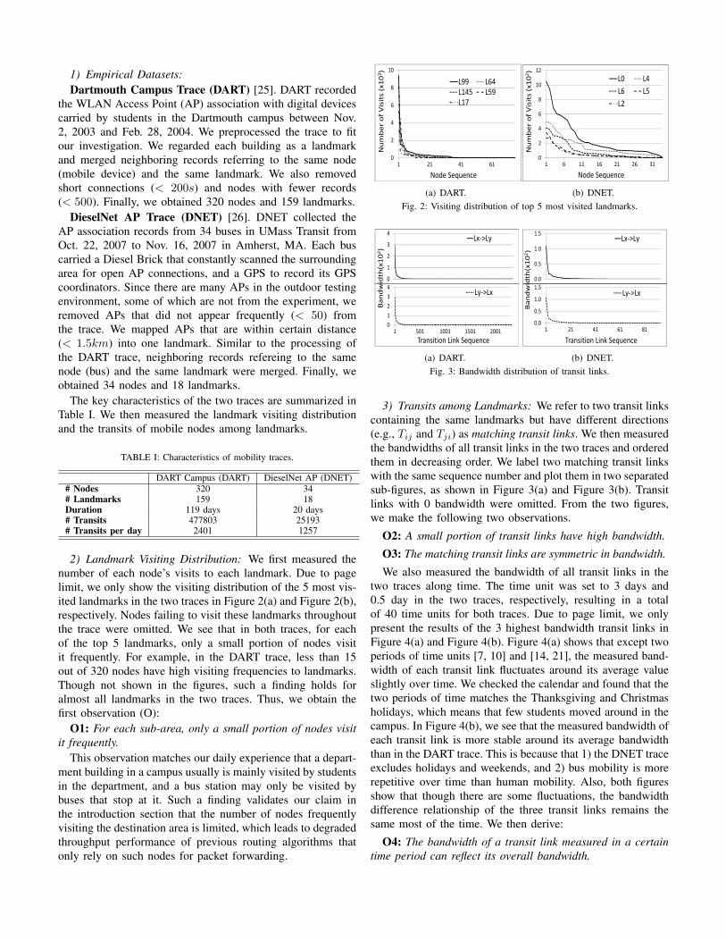
2) Landmark Visiting Distribution: We first measured thenumber of each node’s visits to each landmark. Due to pagelimit, we only show the visiting distribution of the 5 most vis-ited landmarks in the two traces in Figure 2(a) and Figure 2(b),respectively. Nodes failing to visit these landmarks throughoutthe trace were omitted. We see that in both traces, for eachof the top 5 landmarks, only a small portion of nodes visitit frequently. For example, in the DART trace, less than 15out of 320 nodes have high visiting frequencies to landmarks.Though not shown in the figures, such a finding holds foralmost all landmarks in the two traces. Thus, we obtain thefirst observation (O):

O1: For each sub-area, only a small portion of nodes visitit frequently.

This observation matches our daily experience that a depart-ment building in a campus usually is mainly visited by studentsin the department, and a bus station may only be visited bybuses that stop at it. Such a finding validates our claim inthe introduction section that the number of nodes frequentlyvisiting the destination area is limited, which leads to degradedthroughput performance of previous routing algorithms thatonly rely on such nodes for packet forwarding.

0

2

4

6

8

10

1 21 41 61

Number of Visits (x10

3 )

Node Sequence

L99 L64L145 L59L17

(a) DART.

0

2

4

6

8

10

12

1 6 11 16 21 26 31

Number of Visits (x10

2 )

Node Sequence

L0 L4L6 L5L2

(b) DNET.Fig. 2: Visiting distribution of top 5 most visited landmarks.

01234

1 501 1001 1501 2001Transition Link Sequence

Ly‐>Lx

0

1

2

3

4Lx‐>Ly

Bandwidth(x10

2 )

(a) DART.

0.0

0.5

1.0

1.5

1 21 41 61 81

Transition Link Sequence

Ly‐>Lx

0.0

0.5

1.0

1.5Lx‐>Ly

Bandwidth(x10

2 )

(b) DNET.Fig. 3: Bandwidth distribution of transit links.

3) Transits among Landmarks: We refer to two transit linkscontaining the same landmarks but have different directions(e.g., Tij and Tji) as matching transit links. We then measuredthe bandwidths of all transit links in the two traces and orderedthem in decreasing order. We label two matching transit linkswith the same sequence number and plot them in two separatedsub-figures, as shown in Figure 3(a) and Figure 3(b). Transitlinks with 0 bandwidth were omitted. From the two figures,we make the following two observations.

O2: A small portion of transit links have high bandwidth.

O3: The matching transit links are symmetric in bandwidth.

We also measured the bandwidth of all transit links in thetwo traces along time. The time unit was set to 3 days and0.5 day in the two traces, respectively, resulting in a totalof 40 time units for both traces. Due to page limit, we onlypresent the results of the 3 highest bandwidth transit links inFigure 4(a) and Figure 4(b). Figure 4(a) shows that except twoperiods of time units [7, 10] and [14, 21], the measured band-width of each transit link fluctuates around its average valueslightly over time. We checked the calendar and found that thetwo periods of time matches the Thanksgiving and Christmasholidays, which means that few students moved around in thecampus. In Figure 4(b), we see that the measured bandwidth ofeach transit link is more stable around its average bandwidththan in the DART trace. This is because that 1) the DNET traceexcludes holidays and weekends, and 2) bus mobility is morerepetitive over time than human mobility. Also, both figuresshow that though there are some fluctuations, the bandwidthdifference relationship of the three transit links remains thesame most of the time. We then derive:

O4: The bandwidth of a transit link measured in a certaintime period can reflect its overall bandwidth.

0.0

1.0

2.0

3.0

4.0

5.0

6.0

7.0

8.0

0 5 10 15 20 25 30 35 40

Bandwidth (x102)

Time Unit Sequence

L7‐>L99 L145‐>L125L75‐>L78

(a) DART.

0.0

0.5

1.0

1.5

2.0

2.5

3.0

0 5 10 15 20 25 30 35 40

Bandwidth (x102)

Time Unit Sequence

L0‐>L4 L6‐>L0

L5‐>L6

(b) DNET.Fig. 4: The transit distribution of top 3 highest bandwidth transit links.

IV. SYSTEM DESIGN

In this section, we introduce the detailed architectureof our DTN-FLOW system based on above observations. Ithas four main components: (1) landmark selection and sub-area division, (2) node transit prediction, (3) routing tableconstruction, and (4) packet routing algorithm. Component (1)provides general guidelines to select the location of landmarksand split the DTN into sub-areas. Component (2) predicts thenext landmark a node is going to visit based on its previousvisiting records. Such predictions are used to forward packetsand exchange routing tables among landmarks. Component(3) measures the data transfer capacity between each pair oflandmarks, based on which the routing table is built indicatingthe next hop landmark for each destination landmark andassociated estimated delay. With the support of the first twocomponents, component (4) determines the next-hop landmarkand the forwarding node in packet routing.

A. Landmark Selection and Sub-area Division

The landmark selection determines the places to installlandmarks. Sub-area division divides the entire to sub-areaswith each area having one landmark. Both landmark selectionand sub-area division are conducted by the network adminis-trator or planner who hopes to utilize the DTN for a certainapplication.

1) Landmark Selection: As previously introduced, we se-lect popular places that are frequently visited by mobile nodesas landmark places. Therefore, the network administrator firstneeds to identify popular places. A simple way is to collectnode visiting history and take top Nv most frequently visitedplaces as popular places. Popular places in DTNs with socialnetwork structures can be pre-determined based on node mo-bility pattern in the social network. For example, in the DARTnetwork, we can easily find popular buildings that studentsvisit frequently: library, department building, and dorm. InDTNs in rural areas, villages are naturally popular places.In the DTNs using animals as mobile nodes for environmentmonitoring in mountain areas, places with water or foodusually are often visited.

The popular places resulted from both the two ways are putinto the candidate list for landmarks. There may be severalpopular places in a small area. Thus, not every popular placeneeds to be a landmark. Therefore, for every two candidatelandmarks with distance less than Dv meters, the one withless visit frequent is removed from the candidate list. Above

L2 L0L1 L7

L6

L5L4L3

Fig. 5: Sub-area division in our campus deployment.

process is repeated until the distance between every twocandidate landmarks is larger than Dv meters.Nv and Dv decide the number of landmarks and conse-

quently, the sizes of sub-areas. The network administrator canadjust their values so that there are landmarks in most areas ofthe network and in the areas where data is transferred. Basedon our experience, this step can be completed quickly based onthe understanding of node mobility patterns in an applicationscenario, as what we did for the traces in the trace analysispart. We leave the analysis on how Nv and Dv affects therouting performance as our future work.

2) Sub-area Division: With the landmarks, we split theentire network into sub-areas. Since the sub-area division onlyserves the purpose of routing among landmarks, we do notneed a method to precisely define the size of each sub-area.Therefore, we follow below rules to generate sub-areas:

• Each sub-area contains only one landmark.• The area between two landmarks are evenly split to the

two sub-areas containing the two landmarks.• There is no overlap among sub-areas.

Note that the split of area between landmarks does not affecthow nodes move between landmarks. Nodes can transit amonglandmarks through any routes Figure 5 gives an example of thesub-area division in our campus deployment of DTN-FLOW,which is introduced later in Section V-B. With above landmarkselection algorithms, a landmark may be responsible for alarge area while some landmarks may only be responsiblefor a small area. Recall that landmarks are selected frompopular places. Then, a large sub-area is caused by the factthat there is no other popular place in that area. Then, evenwe put extra landmarks in the area, packets cannot reach themquickly since they are not popular places and few nodes visitthem frequently. Therefore, such a design (i.e., uneven sub-area division) does not degrade the routing efficiency but helpsto limit the number of landmarks and save the total cost.

3) Real World Scenarios and Limitations: Above landmarkselection and sub-area division procedures require certainadministration input. However, as previously introduced, thisstep is quite intuitive and requires slight effort. With thedesign of landmarks, we can see that DTN-FLOW is suitablefor DTNs with distributed popular places. In a real-worldDTN, popular places usually are distributed over an area. Forexample, the carrier of mobile devices (i.e., human or animal)usually belong to certain social structures and have skewedand repeated visiting patterns [21]. Also, different nodes have

their own frequently visited places. Therefore, the proposedDTN-FLOW is applicable to most realistic DTN scenarios.

B. Node Transit Prediction

Since DTN-FLOW relies on node transit for packet for-warding, accurate prediction of node transit is a key com-ponent. In DTN-FLOW, each node uses its previous visitinghistory for next transit prediction. Each node maintains alandmark visiting history table as shown in Table II. The “Starttime” and “End time” denote the time when a node connectsand disconnects to the central station in the correspondinglandmark, respectively. Note that the “End time” of visitingprevious landmark is not necessarily the same with the “Starttime” of connecting to current landmark since a node may notalways connect to a landmark during its movement.

TABLE II: Landmark visiting history table in a node.

Landmark ID Start time (s) End time (s)8 8500 90001 7100 84507 2000 7000· · · · · · · · ·

To predict node transits among landmarks, we adopt theorder-k (O(k), k = 0, 1, 2, · · · ) Markov predictor [27], whichassumes that the next transit is only related to the pastk transits. A node’s landmark transit history can be rep-resented by TH = Tx1,x2

Tx2,x3. . . Txj−1,xj

. . . Txn−1,xn, in

which Txj−1,xj(xj−1 6= xj and xj−1, xj ∈ [1,M ]) repre-

sents a transit from Lxj−1to Lxj

. We let X(n − k, n) =Txn−k,xn−k+1

· · ·Txn−1,xnrepresent the past k consecutive

transits. When k = 0, X(n − k, n) = Txn,xn , representingthe visiting of landmark Lxn . Then, the probability for eachpossible next transit Txn,xn+1

of a node is calculated by

Pr(Txn,xn+1 |X(n− k, n)) =Pr(X(n− k, n), Txn,xn+1

)

Pr(X(n− k, n)),

(1)where

Pr(X(n− k, n), Txn,xn+1) = Pr(X(n− k, n+ 1)) (2)

andPr(X(n− k, n)) = N(X(n− k, n))

N(Allk)(3)

where N(X(·)) and N(Allk) denote the number of X(·)and k consecutive transits in TH , respectively. Note N(All0)denotes the number of landmark visits of the node. Then, thetransit that leads to the maximal probability based on Equ. (1)is selected as the predicted transit. For example, supposewe use an order-1 Markov on a system with 5 landmarks(M = 5), and the landmark transit history of a node isTH = T0,1T1,3T3,4T4,2T2,0T0,1. Then, based on Equ. (1), theprobability for each possible next landmark La (a ∈ [1, 5]) iscalculated as Pr(T0,1T1,a)

Pr(T0,1). Suppose a = 3. Based on Equ. (3),

Pr(T0,1T1,3) = 1/5 since T0,1T1,3 appears once in TH andthe total number of 2 consecutive transits is 5. Similarly,Pr(T0,1) = 2/6. Then, the node’s probability of meetinglandmark L3 is 0.67.

We used the order-1 Markov predictor on both DART andDNET traces. Each node makes a prediction for the nextvisiting landmark after each transit based on its past transits.We calculated the accuracy rate of each node, which equalsthe number of correct predictions divided by the number oftotal predictions. The minimal, 1st quantile, average, thirdquantile and maximal of the accuracy rates of all nodes inthe two traces are shown in Figure 6. We see that in theDART trace, the accuracy rates of over 75% of nodes arehigher than 64%, and the average accuracy rate of all nodesis about 77%. In the DNET trace, the accuracy rates ofover 75% of nodes are higher than 59%, and the averageaccuracy rate of all nodes is about 66%. It is intriguing

0.0

0.2

0.4

0.6

0.8

1.0

1.2

Dartmouth Campus DieselNet AP

Accuracy Rate

Fig. 6: The minimal, 1st quantile,average, third quantile, and maximalof the transit prediction accuracy.

to see that the prediction ac-curacy in the bus networkin DNET, which should havemore repetitive moving pat-terns, is lower than that inthe student network on cam-pus in DART. We believe thisis caused by the reason that weonly predict one AP for thenext transit while a bus mayassociate with one of severalneighboring APs after each transit in the trace. Though certaininaccurate predictions exist, the routing efficiency can beensured with a proper handling method that will be explainedin Section IV-D. To increase the accuracy of the transitprediction, we can use the product of the prediction probabilityand the accuracy rate to measure the probability of meeting aspecific landmark.

C. Routing Table ConstructionIn DTN-FLOW, each landmark first dynamically measures

the bandwidths of its transit links to all of its neighbor land-marks. The bandwidth of a transit link represents the expecteddelay of forwarding data through it. Based on the estimateddelay, each landmark uses the distance-vector method [22] tobuild a routing table indicating the next landmark hop for eachdestination landmark that can lead to the minimum estimateddelay. Each landmark periodically transfers its routing tableto its neighbor landmarks, which update their routing tablesaccordingly. The routing table exchange is realized throughmobile nodes based on the prediction of their transits. Thatis, landmark Li chooses its node with the highest predictedprobability of visiting Lj to forward its routing table to Lj .The detailed processes are introduced below.

1) Transit Link Bandwidth Measurement: Each landmarkmaintains a bandwidth table as shown in Table III to recordthe bandwidth from it to each of its neighbor landmarks. Welet N t

ij denote the number of nodes that have moved from Li

to Lj in the t-th time unit. Each landmark, Li, periodicallyupdates its bandwidth to landmark Lj by

Bijnew= αBijold + (1− α)N t

ij (4)

in which Bijnewand Bijold represent the updated bandwidth

and previously measured bandwidth, respectively, and α is a

weight factor.

TABLE III: Bandwidth table in a node.

Landmark ID Measured Bandwidth Time Unit Sequence2 20 96 6 91 15 9· · · · · · · · ·

It is easy for landmark Li to calculate N tji since mobile

nodes moving to Li can report their previous landmarks to Li.However, it is difficult for Li to calculate N t

ij because aftera mobile node moves from Li to Lj , it cannot communicatewith Li. Recall that O3 indicates that two matching transitlinks are symmetric in bandwidths. In this case, Li can regardN t

ij ≈ N tji and calculate Bijnew

using Equ. (4).However, the symmetric property does not always hold true.

For example, transit links connecting two stations in a one wayroad can hardly be symmetric in bandwidth. In this asymmetriccase, each landmark cannot measure the bandwidths of linksfrom it to neighbor landmarks directly. To solve this problem,Li relies on Lj to keep track of Nij . When landmark Lj

predicts that a node is going to leave it for another landmarkLi, it forwards Nij to the node. When Li receives Nij fromLj , it checks whether the time unit sequence in the packetis larger than the one it uses currently. If yes, it updates itsbandwidth to Lj accordingly based on Equ. (4). Otherwise,the packet is discarded.

2) Building Routing Tables: With the bandwidth table, eachlandmark can deduce the expected delay needed to transfer Wbytes of data to each of its neighboring landmarks. Recall Tdenotes the time unit for Bij measurement. Suppose each nodehas S bytes of memory, then the expected delay for forwardinga packet from Li to Lj (Dij) equals Dij = W

BijST . Then,

the routing table on each landmark can be initialized withthe delays to all neighboring landmarks. Each landmark, Li,further uses the distance-vector protocol to construct the fullrouting table (as shown in Table IV) indicating the next hopfor every destination landmark (Ld) in the network and theoverall delay from Li to Ld, denoted by D(Li, Ld).

TABLE IV: Routing table in one node.

Des. Landmark ID Next Hop ID Overall Delay1 1 75 5 39 1 18· · · · · · · · ·

In the distance-vector protocol, each landmark periodicallyforwards its routing table and associated time unit to allneighboring landmarks through mobile nodes. When a land-mark, say Li, receives the routing table from a neighboringlandmark, say Lj , it first checks whether it is newer thanthe previous received one. If not, the table is discarded.Otherwise, the routing table is processed one entry by oneentry. For each entry, if the destination landmark, Ld, doesnot exist in the routing table of Li, it is added to the routingtable by setting the “Next Hop ID” as Lj and the “OverallDelay” as Dij + D(Lj , Ld). If Ld already exists, it checks

Des. ID Next ID Delay

1 1 84 7 207 7 69 7 34

Des. ID Next ID Delay

1 1 83 6 174 6 187 7 69 7 34

3 3 104 3 119 3 30

Original Routing Table on L2

Updated Routing Table on L2

Received Routing Table from L6

Distance from  L2to L6 is 6

Fig. 7: Demonstration of the routing table update.

whether D(Li, Ld) ≤ Dij +D(Lj , Ld). If yes, no change isneeded. Otherwise, the “Next Hop ID” is replaced as Lj andthe “Overall Delay” is updated with Dij + D(Lj , Ld). Thisprocess repeats periodically, and each landmark finally learnsthe next hop to reach each other destination landmark with theminimum overall delay in its routing table.

For example, suppose the routing table on L2 contains fourentries: (1, 1, 8), (4, 7, 20), (7, 7, 6) and (9, 7, 34). It receivesa routing table from L6 with 3 entries: (3, 3, 10), (9, 3, 30), (4,3, 11), and D26=7. Figure 7 summaries the process of routingtable update. In detail, since the routing table of L2 has noentry for landmark L3, it is inserted directly with updatednext hop and delay: (3, 6, 17). Though L9 already exists inthe routing table of L2, D29=34 is less than that of relayingthrough L6 (i.e., 37), so no change is needed. L4 already existsin the routing table, and D24=20 is larger than that of relayingthrough L6 (i.e., 18), so the “Next Hop ID” is changed to 6 and“Overall Delay” is set to 18. The final entries in the routingtable of L2 are (1, 1, 8), (3, 6, 17), (4, 6, 18), (7, 7, 6), and(9, 7, 34).

D. Packet Forwarding AlgorithmDuring the packet forwarding, based on a packet’s des-

tination, a landmark refers to its routing table to select thenext-hop landmark, and forwards the packet to the mobilenode that has the highest predicted probability to transit to theselected landmark. Thus, if node transit prediction is correct,each transit can reduce the expected delay by the maximum.However, as mentioned in Section IV-B, node transit predictionmay not always be accurate, which means a node may carry apacket to another landmark rather than the one indicated in therouting table. Also, there may exist nodes that are moving tothe packet’s destination node directly, which can be utilizedto enhance the routing performance. We first introduce ourapproaches to handle the two issues and then summarize thefinal routing algorithm.

1) Handling Prediction Inaccuracy: To handle the inac-curate transit prediction, DTN-FLOW follows the principlethat every forwarding must reduce the routing latency. Thus,when a node moves from Li to a landmark Lk other thanthe predicted one Lj , the node checks whether the newlandmark still reduces the expected delay to the destinationLd, that is, whether D(Lk, Ld) < D(Li, Ld). If yes, thenode still forwards the packet to landmark Lk for furtherforwarding. Otherwise, the node holds the packet, waiting fornext landmark that has shorter delay to the destination or anode that is predicted to visit Lj soon. This design aims to

ensure that each transit, though may not be optimal due tonode transit prediction inaccuracy, can always improve theprobability of successful delivery.

2) Exploiting Direct Delivery Opportunities: Since nodesmove opportunistically in a DTN, it is possible that a landmarkcan discover nodes that are predicted to visit the destinationlandmarks of some packets. Therefore, when a landmarkreceives a packet, it first checks whether any connected nodesare predicted to transit to its destination landmark. If yes, thepacket is forwarded to the node directly. In case the node failsto forward the packet to its destination landmark, the node usesthe scheme described in Section IV-D1 to decide whether toforward the packet to the new landmark.

3) Routing Algorithm: We present the steps of the routingalgorithm as following.(1) When a node generates a packet for an area, it forwards

the packet to the first landmark it meets.(2) When a landmark, say Li, generates or receives a packet,

it first checks whether any nodes are predicted to moveto the destination landmark of the packet. If yes, thepacket is forwarded to the node with the highest predictedprobability and the expected overall delay, which is usedby the carrier node to determine whether to forward thepacket to an encountered landmark not in prediction.

(3) Otherwise, Li checks its routing table to find the next-hop landmark for the packet and inserts the landmark IDand the expected overall delay into the packet.

(4) Li then checks all connected nodes and forwards thepacket to the node that has available memory and hasthe highest predicted probability to transit to the next-hop landmark indicated by the routing table.

(5) When a node moves to the area of a landmark, say Lj , itforwards Lj all packets that target Lj or have less overalldelay from Lj to the destination than Li. After this, itpredicts its next transit based on the order-k Markovpredictor and informs this to Lj .

V. PERFORMANCE EVALUATION

We first conducted trace-driven experiments with both theDART and the DNET traces and then deployed a small DTN-FLOW system in our campus. We introduce the results of theexperiments in the following.

A. Trace-driven Experiments

1) Experiment Settings: We used the first 1/4 part of thetwo traces as the initialization phase, in which nodes constructrouting tables. Then, packets were generated at the rate ofRp packets per landmark per day. Rp was set to 40 unlessotherwise specified. Each landmark randomly selects anotherlandmark as the destination landmark for its generated packet.We set the TTL (Time to Live) of packets to 20 days in theDART trace and 4 days in the DNET trace. A packet wasdropped after TTL. We set a large TTL in order to betterevaluate the utilization of node movements. The time unit Tfor bandwidth evaluation and routing table update was set to3 days. The size of each packet was set to 1KB, and the sizeof each node’s memory was set to 150KB unless otherwise

specified. The memory in the landmark was not limited. Weused the order-1 Markov predictor in the experiments. We setthe confidence interval to 95%.

We compared DTN-FLOW with three state-of-the-art rout-ing algorithms: SimBet [28], PROPHET [6], and PGR [18].They were originally proposed for node-to-node routing inDTNs. We adapted them to fit landmark-to-landmark routingto make them comparable to DTN-FLOW. We use SimBetto represent the social network based routing methods. Itcombines centrality and similarity to calculate the suitability ofa node to carry packets to a given destination landmark. Cen-trality is calculated based on the ability to connect landmarks,and similarity is derived from the past co-existence recordsabout the frequency that the node visits the landmark. Weuse PROPHET to represent the probabilistic routing methods.It simply employs the encountering records to calculate thefuture meeting probability to guide the packet forwarding. Wemodified the two methods to fit our test scenario by referringthe suitability and probability to a certain landmark. We usePGR to represent the location based routing methods. It usesobserved node mobility routes, described as a sequence oflocations, to check whether the destination landmark is on anode’s route. It then forwards a packet to the node that islikely to move to the destination landmark along its route. Wemeasured following metrics.

• Success rate: The percentage of packets that successfullyarrive at their destination landmarks.

• Average delay: The average time per packet for suc-cessfully delivered packets to reach their destinationlandmarks.

• Forwarding cost: The number of packet forwarding op-erations occurred during the experiment.

• Overall cost: The total number of packet and routinginformation forwarding operations during the experiment.Forwarding a routing table or a meeting probability tablewith m entries is counted as m.

2) Performance with Different Memory Sizes: We firstevaluated the performance of the four methods when the sizeof memory in each node was varied from 100KB to 200KBwith a 20KB increase in each step.

Success Rate: Figure 8(a) and Figure 9(a) present thesuccess rates of the four methods with the DART and theDNET traces, respectively. We see that when the mem-ory in each node increases, the hit rates always followDTN-FLOW>SimBet≈PROPHET>PGR. DTN-FLOW hasthe highest hit rate because it fully utilizes node movementsto forward packets one landmark by one landmark to theirdestination landmarks, even though some nodes rarely or maynot visit these destinations. On the contrary, other methodsonly rely on nodes that visit destinations frequently for packetforwarding. Limited number of such nodes prevent themfrom achieving high success rate. PGR tries to predict theentire route of a node including multiple locations for packetforwarding. However, the accuracy of such a prediction usuallyis low. Recall in Figure 6, the average accuracy rate is alreadybelow 80% for the prediction of only one location. The

0.25

0.30

0.35

0.40

0.45

0.50

100 120 140 160 180 200

Success Rate

Memory Size (KB)

DTN‐FLOW SimBetPROPHET PGR

(a) Success rate.

78

82

86

90

94

98

100 120 140 160 180 200

Average Delay (x10

4 s)

Memory Size (KB)

DTN‐FLOW SimBetPROPHET PGR

(b) Average delay.

5

10

15

20

25

100 120 140 160 180 200

Forw

arding

 Cost (x10

6 )

Memory Size (KB)

DTN‐FLOW SimBetPROPHET PGR

(c) Forwarding cost.

50

100

150

200

250

100 120 140 160 180 200

Total Cost (x10

6 )

Memory Size (KB)

DTN‐FLOW SimBetPROPHET PGR

(d) Total cost.Fig. 8: Performance with different memory sizes using the DART trace.

0.65

0.70

0.75

0.80

0.85

100 120 140 160 180 200

Success Rate

Memory Size (KB)

DTN‐FLOW SimBetPROPHET PGR

(a) Success rate.

7.5

8.0

8.5

9.0

9.5

100 120 140 160 180 200

Average Delay (x10

4 s)

Memory Size (KB)

DTN‐FLOW SimBetPROPHET PGR

(b) Average delay.

0.9

1.2

1.5

1.8

100 120 140 160 180 200

Forw

arding

 Cost (x10

6 )

Memory Size (KB)

DTN‐FLOW SimBetPROPHET PGR

(c) Forwarding cost.

0.0

1.0

2.0

3.0

4.0

100 120 140 160 180 200

Total Cost (x10

6 )

Memory Size (KB)

DTN‐FLOW SimBetPROPHET PGR

(d) Total cost.Fig. 9: Performance with different memory sizes using the DNET trace.

prediction of continuous multiple locations would be lower.Therefore, PGR has the lowest success rate.

PROPHET relies on previous encountering frequency tocalculate the probability of a node to meet a certain land-mark. SimBet exploits social properties, namely centrality andsimilarity, to rank a node’s suitability to carry packets to acertain landmark. Thus, these two methods gradually forwardpackets to their destination landmarks, leading to a relativelyhigh success rate. We also see that SimBet has slightly highersuccess rate than PROPHET in one trace and has similarsuccess rate with PROPHET in another trace. This is becausein addition to meeting probability, SimBet also considerscentrality that measures the activeness of a node to visitdifferent landmarks. Since a node with high centrality maynot have high visiting frequency to the destination landmark,the improvement on the success rate is very small.

We also see that when the memory size increases, thesuccess rates of all the four methods increase. This is becauseeach node can carry more packets and provide more forward-ing services. In summary, the experimental results verify thehigh throughput of DTN-FLOW in transferring data amonglandmarks with difference memory sizes on each node.

Average Delay: Figure 8(b) and Figure 9(b) show theaverage delays of successfully delivered packets in the fourmethods with the DART and the DNET traces, respec-tively. We see that the average delays always follow DTN-FLOW<SimBet≈PROPHET<PGR when memory size in-creases. DTN-FLOW has the lowest average delay becausethe designed routing tables in landmarks guide packets tobe forwarded along the fastest paths to their destinations.For PGR, as explained previously, it is difficult to accuratelypredict long paths with multiple locations, thus leading toinaccurate forwarder selection and the long delay.

In SimBet and PROPHET, packets may be generated inor carried to areas where very few nodes move to their

destinations regularly. Therefore, packets have to wait for acertain period of time before meeting nodes that visit theirdestinations frequently, leading to a moderate average delay.Moreover, since SimBet also considers the centrality. Nodeswith high centrality (i.e., connecting many landmarks) cannotmeet the destination landmarks as frequently as those thathave high meeting probability with the destination landmarksdirectly. Therefore, it generates a slightly higher average delaythan PROPHET.

We also see that when the memory size on each nodeincreases, the average delays of all methods decrease. Largermemory size enables a node to carry more packets from onelandmark, reducing the packets’ waiting time in landmarks.As a result, each packet can be forwarded more quickly,leading to a lower delay. These experimental results showthe high efficiency of DTN-FLOW in transferring data amonglandmarks with difference sizes of memory in each node.

Forwarding Cost: Figure 8(c) and Figure 9(c) plot theforwarding costs of the four methods with the DART andthe DNET traces, respectively. We find that the forwardingcosts follow DTN-FLOW<PGR<SimBet<PROPHET withboth traces. DTN-FLOW refers to the routing table to forwardpackets along fastest landmark paths to reach their destina-tions, which usually takes several forwarding operations.

PGR has the second lowest forwarding cost. This is becausebased on mobility routes, nodes tend to show similar abilityto visit a certain destination. Therefore, a packet holdercannot easily find another node that has higher probability ofmeeting the destination node. Then, packets are not forwardedfrequently. However, the low forwarding cost in PGR alsoresults in a low efficiency.

Both SimBet and PROPHET use a metric to rank thesuitability of nodes for carrying packets and forward packetsto high rank nodes. Then, even when a packet holder meets anode with a slightly higher suitability, it forwards the packet

to the node. As a result, SimBet and PROPHET have higherforwarding cost than PGR and DTN-FLOW. Also, PROPHEThas marginal higher forwarding cost than SimBet. This isbecause higher-centrality nodes usually are a few, leadingto fewer forwarding. On the contrary, PROPHET forwardspackets greedily by only considering meeting frequency.

We further find that when the memory size on each nodeincreases, the forwarding costs of the four methods increase.This is because when each node has more memory, it can carrymore packets and exchange more packets with encounteredlandmarks, resulting in more forwarding cost.

Total Cost: Figure 8(d) and Figure 9(d) plot the total costsof the four methods with the DART and the DNET traces,respectively. We see that with both traces, the total costsfollow DTN-FLOW<PGR<PROPHET<SimBet. Recall thatthe total cost includes packet forwarding cost and maintenancecost, which is incurred by routing information forwarding.In DTN-FLOW, the maintenance cost comes from routingtable updates. When a node connects to a new landmark,it forwards the routing table of its previously connectedlandmark to the new landmark and receives the routing tableof the new landmark. In PGR, PROPHET, and SimBet, twoencountering nodes exchange their calculated suitability/rankfor each destination landmark and then decide whether toforward packets to the other node. Since a node’s probabilityof meeting a landmark is lower than that of meeting anothernode, maintenance cost in DTN-FLOW is less frequent thanthat in other methods. Therefore, DTN-FLOW produces thelowest maintenance cost, and hence the lowest total cost.

Moreover, SimBet has higher maintenance cost than PGRand PROPHET since in addition to the similarity information,nodes in SimBet also need to exchange one more piece ofcentrality information. Comparing Figure 8(d) and Figure 9(d)with Figure 8(c) and Figure 9(c), we notice the maintenancecost is much higher than the forwarding cost. Therefore,SimBet has the highest total cost. PGR and PROPHET haveroughly the same maintenance cost since two encounteringnodes in PGR and PROPHET exchange almost the sameamount of information.

We also see that when the memory size on each nodeincreases, the total costs of all methods remain stable. Thisis because the maintenance cost is much higher than theforwarding cost and is only determined by the number ofencounters among nodes or between nodes and landmarks,which is irrelevant to the memory size in each node. Theresults on forwarding cost and total cost verify the highefficiency of DTN-FLOW in terms of cost with differentmemory sizes on each node.

3) Performance with Different Packet Rates: We also evalu-ated the performance of the four methods with different packetgeneration rates. We varied the packet rate from 20 to 60 with10 increase in each step.

Success Rate: Figure 10(a) and Figure 11(a) show thesuccess rates of the four methods using the DART and theDNET traces, respectively. We see that the success rates followDTN-FLOW>SimBet≈PROPHET>PGR. Such results matchthose in Figure 8(a) and Figure 9(a) for the same reasons.

We also see that when the packet rate increases, the successrates of the four methods decrease. The forwarding oppor-tunities in the system are determined by node memory andencountering opportunities, which are independent with thenumber of packets. When the number of packets increases, thenumber of packets that can be delivered successfully does notincrease accordingly, leading to a degraded success rate. Thehigh success rate of DTN-FLOW with different packet ratesverifies the high throughput performance of DTN-FLOW.

Average Delay: Figure 10(b) and Figure 11(b) illustratethe average delays of the four methods using the DARTand the DNET traces, respectively. We see that the averagedelays follow DTN-FLOW<SimBet≈PROPHET<PGR. Thisrelationship remains the same as in Figure 8(b) and Figure 9(b)for the same reasons. Moreover, we find that when the packetrate increases, the average delays of the four methods increase.This is caused by the limited forwarding opportunities inthe system. When there are more packets in the system, theaverage time a packet needs to wait before being forwardedincreases, resulting in higher total delay. DTN-FLOW alwaysgenerates the lowest average delay at all packets rates, whichdemonstrates the high efficiency of DTN-FLOW in terms ofrouting delay.

Forwarding Cost: Figure 10(c) and Figure 11(c) show theforwarding costs of the four methods using the DART and theDNET traces, respectively. We see that the forwarding costsfollow DTN-FLOW<PGR<SimBet<PROPHET. Again, thisrelationship is the same as in Figure 8(c) and Figure 9(c)due to the same reasons. We also see that the forwardingcosts of the four methods increase when the packet rateincreases. When there are more packets generated in thesystem, more forwarding opportunities are utilized, resultingin more packets forwarding operations. When the packet rateis large enough and all forwarding opportunities are utilizedsufficiently, the forwarding cost would remain stable. This iswhy the forwarding costs in Figure 11(c) remain relative stablewhen the packet rate is larger than 40.

Total Cost: Figure 10(d) and Figure 11(d) show the totalcosts of the four methods using the DART and the DNETtraces, respectively. We see that their total costs again followDTN-FLOW<PGR<PROPHET<SimBet. This result matchesthat in Figure 8(d) and Figure 9(d) for the same reasons. Wealso find that the total costs of the four methods remain quitestable when the packet rates increase. This is because that themaintenance costs of the four methods, which are irrelevant tothe packet rate, dominate the total costs. Such results furtherconfirm the high efficiency of DTN-FLOW in terms of costwith difference packet rates.

Combining all above results obtained with various memorysizes and packet rates, we conclude that DTN-FLOW has su-perior performance in achieving high throughput, low averagedelay, and low cost data transmission between landmarks thanprevious routing algorithms in DTNs.

B. Real Deployment

0.25

0.30

0.35

0.40

0.45

0.50

20 30 40 50 60

Success Rate

Packet Rate 

DTN‐FLOW SimBetPROPHET PGR

(a) Success rate.

78

82

86

90

94

20 30 40 50 60

Average Delay (x10

4 s)

Packet Rate 

DTN‐FLOW SimBetPROPHET PGR

(b) Average delay.

6

12

18

24

30

20 30 40 50 60

Forw

arding

 Cost (x10

6 )

Packet Rate 

DTN‐FLOW SimBetPROPHET PGR

(c) Forwarding cost.

50

100

150

200

250

20 30 40 50 60

Total Cost (x10

6 )

Packet Rate 

DTN‐FLOW SimBetPROPHET PGR

(d) Total cost.Fig. 10: Performance with different packet rates using the DART trace.

0.65

0.70

0.75

0.80

0.85

20 30 40 50 60

Success Rate

Packet Rate 

DTN‐FLOW SimBetPROPHET PGR

(a) Success rate.

7.5

8.0

8.5

9.0

9.5

20 30 40 50 60

Average Delay (x10

4 s)

Packet Rate 

DTN‐FLOW SimBetPROPHET PGR

(b) Average delay.

0.9

1.2

1.5

1.8

20 30 40 50 60

Forw

arding

 Cost (x10

6 )

Packet Rate 

DTN‐FLOW SimBetPROPHET PGR

(c) Forwarding cost.

0.0

1.0

2.0

3.0

4.0

20 30 40 50 60

Total Cost (x10

6 )

Packet Rate 

DTN‐FLOW SimBetPROPHET PGR

(d) Total cost.Fig. 11: Performance with different packet rates using the DNET trace.

Library

L0

Sirren Hall

L1 Riggs HallL2

Union

L3 Brackett Hall

L4Martin Hall

L5

S‐Dining HallL6

Hendrix Center

L7

(a) Map for landmark locations.

Item Value# Landmarks 8# Nodes 9# Transits 147# Packets 2100Duration 4 daysPacket size 1 KB

Node memory 50 KB

(b) Configuration summaryFig. 12: Landmark map and configurations in the real deployment.

1) Settings: We deployed DTN-FLOW in our campus forreal-world evaluation of its performance. We selected 8 build-ings as landmarks and labeled them as L0 to L7. Their locationrelationships are shown in Figure 12(a). Among the 8 land-marks, L0 is the library, L1, L2, L4, and L5 are departmentbuildings, and L3, L6, and L7 are the student center anddining halls. Each of 9 students from 4 departments carried aWindows Mobile phone daily. Each Windows Mobile phonechecks its GPS coordinator periodically to judge whether itis within the area of any landmarks. If yes, it communicateswith the landmark through Wifi.

In the test, each landmark generates 75 packets evenly inthe daytime of each day. We simulated a scenario in whichL0 (Library) needs to collect information from other buildings.Then, all packets were targeted to L0. The TTL of each packetwas set to 3 days. We set the size of each packet to 1KB andthe memory on each node to 50KB. The time unit T was setto 720 minutes. The deployment configuration is summarizedin Figure 12(b).

2) Experimental Results: Figure 13(a) demonstrates thesuccess rate and the minimal, first quantile, average, thirdquantile, and maximal of the delays of successfully delivered

0.0

0.1

0.2

0.3

0.4

0.5

0.6

0.7

0.8

0.9

Success Rate

Percentage

0

5

10

15

20

25

30

35

40

45

Delay

Minutes (x10

2)

(a) Success rate and delay distribution.

L2 L0L1 L7

L6

L5L4L3

0.57

0

0.280.14 0.57

0.57

1.28

1.57 3.28

3.14

0.57

0.420.85

0.710.57

0.43

0.290.29

(b) Bandwidths of transit linksFig. 13: Experimental results in real deployment.

packets. We see that more than 82% of packets were suc-cessfully delivered to the destination. Also, more than 75% ofpackets were delivered within 1400 minutes, and the averagedelay is about 1000 minutes. Note that the entire deploymentonly employed 9 mobile nodes with 147 transits to forwardpackets. A larger deployment with more nodes would increasethe success rate and reduce the delay. These experimentalresults demonstrate the high efficiency of the DTN-FLOW intransferring data among landmarks.

We also obtained the bandwidth of each transit link at theend of the deployment, as shown in Figure 13(b). We omittransit links with bandwidth lower than 0.14 to show the majorrouting paths. We again find that for most pairs of landmarks,the two transit links connecting them are symmetric on band-width. This further confirms our previous observation (O3)in Figure 3(a) and Figure 3(b). The bandwidth on differenttransit links are also within our expectation. For example, thelinks between L0 and L2 have very high bandwidth. This isbecause most students attended the test are from departmentslocated in L2 and L0, and they usually study in the library (L0)and go to classes in both department buildings (L1 and L2).Also, the route between L1 and L0 must go through L2. Suchresults justify that the DTN-FLOW can accurately measure the

amount of transits among landmarks.We further recorded the routing table on each landmark.

Due to page limit, we only show those of L2, L4, and L6

in Table V. We see that the routing tables match the fastestpath based on transit link bandwidths shown in Figure 13(b).For L2, it needs to go through L0 to reach L0, L5, L6, L7.For L4, it relies on L3 and L2 to reach other landmarks. ForL6, except for L7, it has to go through L0 to reach otherlandmarks. Such results verify that the routing table updatein DTN-FLOW, which relies on mobile nodes, is reliable andcan reflect the suitable paths to each destination.

TABLE V: Routing tables in L2, L4, and L6.

Landmark ID Destination Landmark Next-hop

L2

L0, L5, L6, L7 L0

L1 L1

L3 L3

L4 L4

L4L0, L1, L3, L6, L7 L3

L2, L5 L2

L6L0, L1, L2, L3, L4, L5, L6 L0

L7 L7

VI. CONCLUSION

In this paper, we propose DTN-FLOW, an efficient routingalgorithm to transfer data among landmarks for high through-put in DTNs. DTN-FLOW splits the entire DTN area into sub-areas with different landmarks, and uses node transits betweenlandmarks to forward packets one landmark by one landmarkto reach their destinations. Specifically, DTN-FLOW consistsof four components: landmark selection and sub-area division,node transit prediction, routing table construction, and packetrouting algorithm. The first component selects landmarks fromplaces that are frequently visited by nodes and split thenetwork work into sub-areas. The second component predictsnode transits among landmarks based previous movementsusing the order-k Markov predictor. The third componentmeasures the transmission capability between each pair oflandmarks, which is used to build routing tables indicatingthe next landmark hop to each destination. The routing tableexchange among landmarks for routing table update is realizedthrough mobile nodes. In the fourth component, each landmarkdecides the next-hop landmark for each packet by checkingits routing table and forwards the packet to the node withthe highest probability of meeting the landmark. We haveanalyzed two real traces to verify the shortcoming of previousDTN routing algorithms and hence confirm the motivation anddesign of DTN-FLOW. We also deployed a small DTN-FLOWsystem in our campus. The experimental results from the realdeployment and extensive trace-drive simulation prove thehigh efficiency and throughput of DTN-FLOW compared withdifferent previous routing algorithms in DTNs. In the future,we plan to investigate how to combine node-to-node commu-nication to further enhance the packet routing efficiency.

ACKNOWLEDGEMENTS

This research was supported in part by U.S. NSFgrants CNS-1254006, CNS-1249603, CNS-1049947, CNS-1156875, CNS-0917056 and CNS-1057530, CNS-1025652,

CNS-0938189, CSR-2008826, CSR-2008827, Microsoft Re-search Faculty Fellowship 8300751, and U.S. Departmentof Energy’s Oak Ridge National Laboratory including theExtreme Scale Systems Center located at ORNL and DoD4000111689.

REFERENCES

[1] S. Jain, K. R. Fall, and R. K. Patra, “Routing in a delay tolerant network,”in Proc. of SIGCOMM, 2004.

[2] K. Fall, “A delay-tolerant network architecture for challenged internets,”in Proc. of SIGCOMM, 2003.

[3] P. Juang, H. Oki, Y. Wang, M. Martonosi, L. S. Peh, and D. Rubenstein,“Energy-efficient computing for wildlife tracking: Design tradeoffs andearly experiences with ZebraNet,” in Proc. of ASPLOS-X, 2002.

[4] A. Vahdat and D. Becker, “Epidemic routing for partially-connected adhoc networks,” Duke University, Tech. Rep., 2000.

[5] Y. Tseng, S. Ni, and E. Shih, “Adaptive approaches to relieving broadcaststorms in a wireless multihop mobile ad hoc network.” in Proc. ofICDCS, 2001.

[6] A. Lindgren, A. Doria, and O. Schelen, “Probabilistic routing in inter-mittently connected networks.” Mobile Computing and CommunicationsReview, vol. 7, no. 3, 2003.

[7] J. Burgess, B. Gallagher, D. Jensen, and B. N. Levine, “MaxProp:Routing for vehicle-based disruption-tolerant networks,” in Proc. ofINFOCOM, 2006.

[8] A. Balasubramanian, B. N. Levine, and A. Venkataramani, “DTN routingas a resource allocation problem.” in Proc. of SIGCOMM, 2007.

[9] K. Lee, Y. Yi, J. Jeong, H. Won, I. Rhee, and S. Chong, “Max-Contribution: On optimal resource allocation in delay tolerant networks.”in Proc. of INFOCOM, 2010.

[10] F. Li and J. Wu, “MOPS: Providing content-based service in disruption-tolerant networks,” in Proc. of ICDCS, 2009.

[11] P. Hui, J. Crowcroft, and E. Yoneki, “Bubble rap: social-based forward-ing in delay tolerant networks,” in Proc. of MobiHoc, 2008.

[12] E. M. Daly and M. Haahr, “Social network analysis for routing indisconnected delay-tolerant manets,” in Proc. of MobiHoc, 2007.

[13] E. Yoneki, P. Hui, S. Chan, and J. Crowcroft, “A socio-aware overlay forpublish/subscribe communication in delay tolerant networks,” in Proc.of MSWiM, 2007, pp. 225–234.

[14] P. Costa, C. Mascolo, M. Musolesi, and G. P. Picco, “Socially-awarerouting for publish-subscribe in delay-tolerant mobile ad hoc networks,”IEEE JSAC, vol. 26, no. 5, pp. 748–760, 2008.

[15] B. Chiara and et al., “Hibop: A history based routing protocol foropportunistic networks,” in Proc. of WoWMoM, 2007.

[16] J. Link, D. Schmitz, and K. Wehrle, “GeoDTN: Geographic routing indisruption tolerant networks,” in Proc. of GLOBECOM, 2011.

[17] A. Sidera and S. Toumpis, “DTFR: A geographic routing protocol forwireless delay tolerant networks,” in Proc. of Med-Hoc-Net, 2011.

[18] J. Kurhinen and J. Janatuinen, “Geographical routing for delay tolerantencounter networks,” in Proc. of ISCC, 2007.

[19] I. Leontiadis and C. Mascolo, “GeOpps: Geographical opportunisticrouting for vehicular networks,” in Proc. of WOWMOM, 2007.

[20] J. Lebrun, C. nee Chuah, D. Ghosal, and M. Zhang, “Knowledge-basedopportunistic forwarding in vehicular wireless ad hoc networks,” in Proc.of VTC, 2005.

[21] J. Leguay, T. Friedman, and V. Conan, “DTN routing in a mobilitypattern space,” in Proc. of WDTN, 2005.

[22] C. Hedrick, “RFC1058 - Routing Information Protocol,” 1988.[23] K. C. Lee, M. Le, J. H0Ł1rri, and M. Gerla, “Louvre: Landmark overlays

for urban vehicular routing environments.” in Proc. of VTC Fall, 2008.[24] A. G. Valko, “Cellular IP: A new approach to internet host mobility,”

ACM Computer Comminication, 1999.[25] T. Henderson, D. Kotz, and I. Abyzov, “The changing usage of a mature

campus-wide wireless network,” in Proc. of MOBICOM, 2004.[26] A. Balasubramanian, B. N. Levine, and A. Venkataramani, “Enhancing

interactive web applications in hybrid networks,” in Proc. of MOBICOM,2008.

[27] L. Song, D. Kotz, R. Jain, and X. He, “Evaluating location predictorswith extensive wi-fi mobility data,” in Proc. of INFOCOM, 2004.

[28] E. M. Daly and M. Haahr, “Social network analysis for routing indisconnected delay-tolerant MANETs,” in MobiHoc, 2007.