drag force on a particle straddling a fluid interface
TRANSCRIPT

HAL Id: hal-03162438https://hal.archives-ouvertes.fr/hal-03162438
Submitted on 8 Mar 2021
HAL is a multi-disciplinary open accessarchive for the deposit and dissemination of sci-entific research documents, whether they are pub-lished or not. The documents may come fromteaching and research institutions in France orabroad, or from public or private research centers.
L’archive ouverte pluridisciplinaire HAL, estdestinée au dépôt et à la diffusion de documentsscientifiques de niveau recherche, publiés ou non,émanant des établissements d’enseignement et derecherche français ou étrangers, des laboratoirespublics ou privés.
Drag force on a particle straddling a fluid interface:Influence of interfacial deformations
J. -C. Loudet, M. Qiu, J. Hemauer, J. Feng
To cite this version:J. -C. Loudet, M. Qiu, J. Hemauer, J. Feng. Drag force on a particle straddling a fluid interface:Influence of interfacial deformations. European Physical Journal E: Soft matter and biological physics,EDP Sciences: EPJ, 2020, 43 (2), �10.1140/epje/i2020-11936-1�. �hal-03162438�
Drag force on a particle straddling a fluid interface: influence of
interfacial deformations
Loudet J.-C.†,‡,1, Qiu M.‡,, Hemauer J.‡,, and Feng J.J.‡,
†University of Bordeaux, CNRS, Centre de Recherche Paul Pascal (UMR 5031),
F-33600 Pessac, France
‡University of British Columbia, Department of Mathematics, Vancouver, BC, V6T 1Z2,
Canada
Abstract
We numerically investigate the influence of interfacial deformations on the drag
force exerted on a particle straddling a fluid interface. We perform finite element
simulations of the two-phase flow system in a bounded two-dimensional geometry.
The fluid interface is modeled with a phase-field method which is coupled to the
Navier-Stokes equations to solve for the flow dynamics. The interfacial deformations
are caused by the buoyant weight of the particle, which results in curved menisci.
We compute drag coefficients as a function of the three-phase contact angle, the
viscosity ratio of the two fluids, and the particle density. Our results show that, for
some parameter values, large drag forces are not necessarily correlated with large
interfacial distortions and that a lower drag may actually be achieved with non-flat
interfaces rather than with unperturbed ones.
Keywords: Two-phase flows, particle/fluid flow, fluid interface, phase-field sim-
ulations, interfacial deformations, drag force.
[email protected] or [email protected]
1

1 Introduction
The problem of particles straddling an interface between two immiscible fluids (e.g. oil
and water or air and water) has been extensively addressed in the literature for many
decades. It is well-established that the presence of a fluid interface alters drastically the
transport properties of adsorbed particles (e.g. macromolecular proteins, small Brownian
aggregates, or macroscopic objects) and their interactions compared to the bulk situation.
For instance, in addition to bulk interactions due to van der Waals and electrostatic
forces, floating particles may also experience capillary interactions if they cause sufficient
perturbations in the interfacial shape [1, 2]. Such interactions originate from the overlap
of interfacial distortions and feature energies well above the thermal energy that may lead
to the clustering of a great variety of particles (from 10 nm to 1 cm) forming a wide range
of self-assembled structures [1, 3, 4]. Other experiments revealed that the diffusivity of
Brownian interfacial particles may be at odds with the well-known bulk Stokes-Einstein
law [5].
Early investigations of interfacial particle hydrodynamics dealt with translational mo-
tions both across and along fluid phase boundaries combined with rotations about axes
lying in the interfacial plane [6]. One of the simplest situations deals with the drag force
FD exerted on an isolated rigid sphere translating along a fluid interface at low Reynolds
number. In this case, FD has been written as [7]:
FD = −6πµRfdU , (1)
where R is the sphere radius, µ denotes a characteristic dynamic viscosity, U is the
particle velocity relative to the fluids, and fd is a corrective dimensionless drag coefficient
accounting for the presence of the interface. The well-known bulk Stokes drag is obviously
recovered for fd = 1. However, this is seldom the case at the interface where fd can be
either smaller or greater than 1. Several experimental and theoretical studies have shown
that fd depends not only on the three-phase contact angle α and the viscosity ratio of the
two fluids [7, 8, 9, 10, 11, 12, 13], but also on the deformation of the interface which in turn
is a function of the fluids density ratio, surface tension, size and density of the adsorbed
2

particle [14]. The presence of adsorbed surfactants brings in an additional contribution to
the drag, with fd up to ≃ 3, due to the viscous nature of the interface with nonvanishing
shear and dilatational viscosities [8, 9, 15, 16, 17]. More recent investigations focused
on the influence of contact line fluctuations on the drag force [18, 19], whereas both the
rotational and translational dynamics of a colloid moving at a flat air-liquid interface in
a thin film were addressed in [20].
However, among the various parameters affecting the value of fd, the influence of
interfacial deformations has been particularly overlooked so far. On the experimental
side, Petkov et al. [14] were the first to address this issue and reported substantial fd
values (fd ≃ 1.75) due to a deformed meniscus forming around heavy copper spheres
translating at the air-water interface. The meniscus dimple was caused by the particle
buoyant weight in this case and the authors attributed the enhanced drag coefficient
to the motion of the curved meniscus around the particle together with the particle
itself. So far, we are unaware of any other study similar to that of [14] at liquid-gas
interfaces. However, a few works dedicated to pairwise interactions of interfacial particles
at liquid-liquid interfaces mentioned smaller fd values, around 1.2, presumably for the
same reasons [21, 22, 23]. On the theoretical side, only the recent work of Dorr & Hardt
[24] considered explicitly interfacial deformations around spherical particles translating
along an interface between fluids of very different viscosities. The driven spheres act as
capillary dipoles but the effect on the drag force was not reported. Furthermore, we
are not aware of any numerical simulations that take explicitly into account interfacial
perturbations. Does a curved meniscus always increase the drag, as is commonly believed?
A detailed investigation on that subject is currently missing and will be the main topic
of the present work. Since drag forces are ubiquitous in any fluid media, the problem is
also relevant to the self-assembling properties of a great variety of adsorbed species (e.g.
nano- or micro-particles, proteins, molecular aggregates) confined in fluid interfaces, thin
liquid films, and even membranes of lipid vesicles or living cells [4].
In the following, we wish to shed some light on the influence of interfacial deformations
on the drag force exerted on particles translating along a fluid interface. We tackle this
3

task through two-dimensional (2D) numerical simulations able to describe the dynamics
of two-phase flow systems in the presence of a fluid interface and a three-phase contact
line. Our primary objective is to qualitatively capture the main physical trends upon
browsing the parameter space, which justifies a simple 2D approach to start with. To
the best of our knowledge, we do not know of any other simulations or theoretical works
addressing similar issues.
The outline of the paper is as follows. In section 2, we describe the geometry of
the problem prior to summarizing the governing equations in section 3. We specify the
relevant dimensionless parameters along with some details relative to the computations
of drag forces and particle densities. General considerations on the numerical method
we employed follow in section 4. Validation steps are then presented in section 5 before
describing and discussing the results in section 6. In particular, we will show that large
drag forces are not necessarily correlated with large interfacial deformations. Concluding
remarks close the paper in section 7.
2 Geometry
The detailed geometry of our 2D problem is specified in Fig. 1. An infinitely long circular
cylinder of radius R and density ρp is trapped at the interface between two Newtonian
fluids of different densities (ρ1, ρ2 with ρ2 > ρ1) and dynamic viscosities (µ1, µ2). The
whole system is confined in a box of length L and height H. In practice, the cylinder
moves horizontally across the interface with a constant velocity −U0 x under the action of
an external force. However, in our simulations, we use a reference frame attached to the
cylinder so that far from it, both liquids flow with constant velocity U0 in the direction of
the x-axis. In this case, the upper and lower bounding plane walls should also move with
the same velocity U0 from left to right in their own planes. Note that the cylinder’s center
of mass will not be necessarily located midway across the fluid interface. Actually, its
position will be shifted either up or down in order to simulate different cylinder densities,
as we will explain further below. In most cases, the fluid interface will be deformed
around the cylinder, featuring either an upward or a downward meniscus depending on
4
operating conditions. The interfacial tension between the two fluids is denoted as σ.
The fluid interface is kept horizontal at the inlet and the outlet in all cases, whereas the
contact angle, α, at the cylinder surface (cf. Fig. 1) is a parameter of the simulation
which will take on different values. All the physical and geometrical parameters used in
the simulations are reported in table 1.
Figure 1: Geometry of the problem for the computation of two-dimensional two-phase flow
drag on a circular cylinder confined at a fluid interface between two plane walls. PPC: Pressure
Point Constraint, α: contact angle, ∆ym: Meniscus elevation. See text and table 1 for other
symbol definitions.
3 Governing equations
3.1 Two-phase flow modeling
In order to determine the drag force exerted on the cylinder at the fluid interface, we need
a model able to describe the interfacial dynamics accurately. Among the numerous multi-
phase flow approaches available in the literature [25], we opted for a diffuse interface
method, based on the concept of “phase-field” (PF), to account for the fluid interface
motion, combined with the Navier-Stokes equations to describe the flow. The choice
of the PF model was primarily motivated by the fact it provides an elegant, coarse-
grained physical description of interfaces where short-range intermolecular interactions,
5

Table 1: Definitions and values of the parameters used in the simulations.
Parameter Symbol Value Unit
Cylinder radius R 1 mm
Box length L 30R mm
Box height H 20R mm
Inlet/outlet velocity U0 20 µm.s−1
Upper fluid dynamic viscosity µ1 0.001− 0.1 Pa.s
Lower fluid dynamic viscosity µ2 0.1 Pa.s
Upper fluid density ρ1 800− 103 kg.m−3
Lower fluid density ρ2 103 kg.m−3
Cylinder density ρp 600− 1200 kg.m−3
Interfacial tension between fluids 1 and 2 σ 0.01 N.m−1
Contact angle α 40◦ − 140◦ deg
such as van der Waals forces, are implicitly taken into account. An explicit tracking of
the fluid interface is unnecessary and the interface normal and curvature are not required
to accurately determine surface tension forces. Moreover, the PF approach is naturally
able to simulate contact line motion without any singularity or ad hoc slip models [25].
The details of the coupled phase-field/Navier-Stokes equations have been described ex-
tensively by a number of authors [25, 26, 27, 28]. Consequently, in the following, we will
only highlight the main ideas and list the governing equations.
The two fluid components are considered immiscible, but in the PF formulation, they
are allowed to mix within a thin interfacial region. A PF variable, or scaled ‘concentra-
tion’, ϕ is introduced such that in the two-fluid bulks ϕ = ±1 and the fluid-fluid interface
is defined by ϕ = 0. The free energy associated with the mixing process may be written
fmix =λ
2|∇ϕ|2 + λ
4ϵ2(ϕ2 − 1
)2, (2)
where λ is the mixing energy density with a dimension of force, and ϵ is a capillary width
6
representative of the diffuse interface thickness. The equilibrium fluid-fluid interfacial
tension is defined by the ratio λ/ϵ and given by [26, 27]
σ =2√2
3
λ
ϵ. (3)
The evolution of ϕ, and therefore of the fluid interface, is governed by the Cahn-Hilliard
(CH) equation [26, 27]∂ϕ
∂t+ v ·∇ϕ = ∇ · (γ∇G) , (4)
where G = λ[−∇2ϕ+ (ϕ2 − 1) /ϵ2
]is the chemical potential, γ the mobility parameter
(assumed to be constant), and v the fluid velocity. The balance equations of mass and
momentum must be added to the above relation to describe the fluid dynamics. The fluids
being incompressible, the velocity and pressure fields satisfy the Navier-Stokes equations
∇ · v = 0 , (5)
ρ(ϕ)
(∂v
∂t+ v ·∇v
)= −∇p+∇ · σv + ρ(ϕ)g +G∇ϕ , (6)
where the last body force term in the momentum relation (G∇ϕ) is the diffuse-interface
equivalent of the interfacial tension [26, 29]. σv = µ(ϕ)[∇v + (∇v)T
]is the viscous
stress tensor, g is the gravitational acceleration, and ρ(ϕ) (resp. µ(ϕ)) is the density
(resp. the viscosity) of the two-phase system given by: ρ(ϕ) = 1+ϕ2ρ1 + 1−ϕ
2ρ2 , and
µ(ϕ) = 1+ϕ2µ1 +
1−ϕ2µ2 .
The coupled equations (4-6) must be supplemented by initial and boundary conditions.
With the help of Fig. 1, the boundary conditions for the velocity are:
v = U0 x , onΓwall (7)
v = 0 , on the cylinder (Γp) (8)
v = U0 x , onΓin and Γout . (9)
The pressure level was set to zero at the top left corner of the box [pressure point
constraint (ppc) in Fig. 1]. As for the CH variables, we impose the following boundary
7

conditions for the chemical potential (G) and ϕ
∇G · n = 0 , on all boundaries (10)
∇ϕ · n = |∇ϕ| cosα , at the contact line (11)
∇ϕ · n = 0 , on Γin and Γout , (12)
where n is the outward unit normal vector to the considered boundary. Eq. (10) is a
zero-flux natural boundary condition resulting from the variational formulation of the
CH equation. Eq. (11) is a geometric condition enforcing a constant contact angle α at
the three-phase contact line on the cylinder. This condition is set in the Comsol phase-
field module and allows the determination of the contact line position. The latter is
automatically updated according to the motion of the fluid interface. Also, we assume
that equilibrium is reached at any time so that contact angle hysteresis is discarded.
Outside of the fluid interface, Eq. (11) reduces to a homogeneous Neumann condition,
while Eq. (12) simply reflects the fact that we impose α = 90◦ on Γin and Γout .
Finally, as initial conditions, we set up a zero pressure and fluid velocity everywhere
in the domain. At time t = 0, the fluid interface is flat and the particle center of mass
lies in the center of the box, if not otherwise stated.
3.2 Dimensionless groups
If we consider the parameters listed in table 1, together with those specific to the CH
model, namely, the capillary width ϵ and the interfacial mobility γ, a total of seven
8

dimensionless numbers may be constructed for our problem:
Bo =∆ρgR2
σ, where ∆ρ = ρ2 − ρ1 (Bond number) (13)
Ca =µ2U0
σ, (capillary number) (14)
Re =ρ2U0R
µ2
, (Reynolds number) (15)
Cn =ϵ
R, (Cahn number) (16)
S =
√γµe
R, where µe =
√µ1µ2 (mobility number) (17)
µ∗ =µ1
µ2
, (viscosity ratio) (18)
ρ∗ =ρ1ρ2
, (density ratio) . (19)
The Bond number, Bo, compares the relative importance of surface tension and gravity
forces. It may also be written as: Bo = (R/Lc)2, where Lc =
√σ/(g∆ρ) is the capillary
length. The latter gives the typical length scale over which interfacial deformations occur
due to the competition between surface tension and gravity. In our work, Bo will be
smaller than unity (Bo ≃ 0.2), meaning that capillarity will be more important than
gravity. The capillary number will be very small in this study, Ca ∼ 10−4 − 10−3,
implying that the shape of the fluid interface should not be altered by the flow around the
cylinder. This is the simplest situation to consider as a first step and, given the already
complicated nature of the problem, we will not explore here the effect of finite Ca, which
can be examined in a future effort. Moreover, since the cylinder is kept fixed and does not
rotate, and that all our drag simulations involve steady-state flows, there is no motion of
the contact line relatively to the cylinder surface.
Next, fluid inertia is not important here since the Reynolds number is well below unity
(Re ∼ 10−4−10−3), i.e. we are near the Stokes flow limit. The two following dimensionless
groups, Cn and S, are specific to the CH model. The former represents the interfacial
thickness while the latter reflects the so-called CH-diffusion across the fluid interface [30].
Their values cannot be easily assigned for real materials but are of paramount importance
to ensure convergence and accuracy of the computed solutions. We used the guidelines
proposed in [29, 30] to ensure that the fluid interface was appropriately resolved, which is
9

a crucial issue in the PF method. More details on this point will be provided in the next
section. Finally, we varied the viscosity ratio in the range 0.01− 1 while the density ratio
was kept close to unity (0.8− 1).
3.3 Drag force and particle density calculations
In our 2D geometry (Fig. 1), the drag force (per unit length), FD, acting on the particle
in the x-direction, can be computed by integrating the total stress exerted on the cylinder
contour, Γp ,
FD = x ·∮Γp
(−pI+ σv) · n ds , (20)
where x is the unit vector in the x-direction, n the outward unit normal vector on the
line element ds, and σv the viscous stress tensor defined previously [Eq. (6)]. Since we
only consider the case of a nonviscous fluid interface, there is no additional contribution
coming from the fluid interface to the drag force. The influence of interfacial viscosity on
FD was considered by, e.g. Danov et al. [8, 9].
In our simulations, the interfacial deformations are caused by the particle’s buoyant
weight which depends on its density. At steady state, the y-component of the force balance
on the particle reads:
Mg = Fv + Fc = y ·∮Γp
(−pI+ σv) · n ds+ σ y ·∮Γp
σc · n ds , (21)
where M is the mass (per unit length) of the cylinder and y is the unit vector in the
y-direction. σc is the capillary stress tensor whose expression can be derived using a
variational procedure, as shown in [27], yielding
σc = fmix I− λ∇ϕ∇ϕ , (22)
where fmix is the mixing free energy density defined in Eq. (2). Note that taking the
divergence of Eq. (22) leads exactly to the body force term (G∇ϕ) in Eq. (6) for the
surface tension. The first term on the right hand side (rhs) of Eq. (21) accounts for
the viscous force (per unit length), Fv, exerted on the particle due to stresses generated
10
by fluid motion. In the absence of flow, Fv simply reduces to the buoyancy force. The
second term on the rhs of Eq. (21) corresponds to the capillary force (per unit length),
Fc , exerted on the cylinder because of interfacial deformations. Note that Fc becomes
non-zero as soon as the interface deforms to satisfy the prescribed contact angle for a given
position of the cylinder across the interface. Since Fv and Fc can be readily computed in
the simulations, the particle weight (or density) follows directly from Eq. (21).
In this work, we would like to stress that we choose to explore the effect of different
particle densities not by tuning the value itself, but by changing the vertical position of
the particle across the interface. For a given contact angle, we compute the steady state
solution while holding the cylinder fixed in place and compute its density as explained
above. We will demonstrate in Sec. 5.2 that the resulting interfacial profile is identical to
that one would obtain by solving explicitly the vertical force balance [Eq. (21)] for a freely
moving cylinder of the same density. In the latter case, the cylinder would be allowed to
translate vertically across the interface until equilibrium is reached, and a costly moving
mesh feature would be required to resolve this motion in situ. Our strategy enables us to
bypass this complication, thereby making the computations faster.
Finally, it will be shown in Sec. 6.3 that the explored range of particle displacements
across the interface does not incur any change in confinement effect.
4 Numerical method
Eqs. (4)-(6), and the imposed boundary conditions [Eqs. (7)-(12)], were solved numeri-
cally using the finite element computational software COMSOL Multiphysicsr [31] with
the coupled two-phase laminar flow/phase-field (Cahn-Hilliard) modules. To guarantee
accuracy and stability, we discretized the fluid flow with quadratic elements for the ve-
locity field and linear elements for the pressure field; quadratic elements were employed
to discretize the phase-field variable. We used a fixed nonuniform triangular mesh fitted
with subdomains to appropriately resolve the fluid interface as it moved within the do-
main to satisfy the imposed contact angle on the cylinder surface. The subdomains were
uniformly meshed with a mesh size adjusted so that the interfacial thickness, which is on
11

the order of 4ϵ, contained at least 8− 10 elements. According to the criterion defined in
[29, 30], the latter condition ensures a sufficient resolution of the fluid interface, which is
of great importance within the PF framework. The dimensions of the subdomains were
optimized in each case, depending on the contact angle value and the vertical position of
the cylinder. Sizeable interfacial deformations, which mostly occurred for small (α < 50◦)
and large (α > 130◦) contact angles, required the largest subdomains, as expected. Out-
side of these domains, the mesh size was much coarser since the fluid interface never
wandered in these areas. The value of the mobility number S was adjusted so that the
inequality Cn < 4S was always satisfied in all our simulations. The latter condition was
recommended as a guideline in [30] for producing convergent results with moving contact-
lines. With a Cahn number Cn = 0.04 (resp. Cn = 0.02), a typical mesh consisted of
≃ 140 000 (resp. 450 000) elements with about 1.5 million (resp. 4.8 million) degrees of
freedom. We advanced the system to steady state using an implicit time-stepping scheme.
At every time step, we used Newton iterations to solve the nonlinear system, and chose
either the ‘MUMPS’ or ‘PARDISO’ solver of COMSOL to solve linear systems. Steady
state was reached, in most cases, after ∼ 50 s (physical time) and about 1h (Cn = 0.04)
to 4h (Cn = 0.02) of computing time on a workstation equipped with an Intel i7 8-core
processor with 64 GB of RAM.
5 Validations
5.1 Drag force
Prior to dealing with non-flat interfaces, we first present a validation of our numerical
setup for computing the drag force on the cylinder in a confined two-phase flow case
with a flat interface. Since the simulation box has a finite size, confinement effects are
unavoidable, and it is well-known that the presence of boundaries strongly influence drag
values [32]. Nevertheless, the confined case is still very interesting to consider because,
one the one hand, experimental systems are always confined, and on the other hand, the
so-called Stokes’ paradox [33] disappears in a bounded geometry, allowing 2D Stokes drag
12

Table 2: Comparison between our numerical results and those of the literature for the dimen-
sionless drag force FD. Definition of symbols: H/L: Box aspect ratio; spf: single-phase flow;
tpf: two-phase flow. Rel. err.: Relative error between Present Study - spf and Present Study
- tpf. Cn: Cahn number [cf. Eq. (16)]. For the Present Study - tpf case, the two phases
have the same viscosity and density than in the Present Study - spf situation. For illustrative
purposes, only the results for two different values of H/L are displayed below, but many other
degrees of confinement were tested and show an equally good agreement between the litera-
ture data and our simulations. Parameters: µ = 0.1Pa.s, ρ = 103 kg.m−3, U0 = 20µm.s−1,
Re = 2× 10⁻⁴.
FD = FD/µU0H/L
Ref. [35] Ref. [34] Present Study - spf Present Study - tpf Rel. err. (%)
8.9650 (Cn = 0.04) 0.26
8.9535 (Cn = 0.02) 0.1320R/30R 9.1990 8.9506 8.9440
8.9400 (Cn = 0.01) 0.02
16.5555 (Cn = 0.04) 0.25
16.5155 (Cn = 0.02) 0.1210R/20R 16.7335 16.5326 16.5160
16.5080 (Cn = 0.01) 0.05
analytical solutions to be found [34]. However, since we were unable to find any reference
data for two-phase flows in a confined geometry, we used as references the analytical
result of Faxen [34] and the numerical data of Ben Richou et al. [35] valid for single-phase
flows and very low Re. To compare with such data, we computed the bulk flow around
a cylinder, first using a single-phase formalism, and then employing our more general
two-phase formalism. In the latter case, we matched the densities and viscosities of the
two phases so that the fluid interface plays no role. In these tests, the cylinder lies in
the middle of the box with the fluid interface (when present) halving the domain. In
two-phase flows, a 90◦-contact angle was imposed on all solid boundaries. We computed
the dimensionless drag force FD = FD/µU0 for two box aspect ratios H/L. The values
are summarized in table 2, along with the other relevant parameters.
13

Figure 2: Velocity field and the associated streamlines (red arrow lines) obtained for (A) a
single-phase flow (spf) (reference state), and (B) a two-phase flow (tpf) with the cylinder held
fixed in the middle of the box. The fluid interface is represented as a solid black line (ϕ = 0)
and the color bar indicates the velocity amplitude in m/s. Simulation parameters: α = 90◦
(tpf), µ∗ = 1 (tpf), ρ∗ = 1 (tpf), Cn = 0.01 (tpf), H/L = 20R/30R.
As can be seen from table 2, our single-phase flow values for FD reproduce well the
literature data, especially those due to Faxen [34]. The same comment goes for the
two-phase flow situation with identical phases. The relative error on FD is on the order
of 0.25% or less depending on the Cahn number. As Cn decreases, the two-phase flow
value of FD becomes extremely close to its single-phase flow counterpart, meaning that we
approach the so-called sharp interface limit (ϵ → 0) [29, 30]. In this limit, the CH diffusion
is minute, the fluid interface is at equilibrium and does not perturb the streamlines, which
should be identical (with α = 90◦) to those of the single-phase flow case, as is indeed
revealed in Fig. 2. The overall good agreement therefore validates our numerical setup.
In the following, we will use the box size H/L = 20R/30R to make sure that (i) the
position of the confining walls is not too close to the cylinder, i.e. we are not dealing with
a highly confined geometry, and (ii), the lateral extension of the fluid interface covers
a few times the capillary length in most cases. Note that increasing the length of the
simulation box is computationally costly since the fluid interface has to be finely resolved
within the PF method. For H = 20R, we have checked that increasing L further has
14

no consequence on the value of FD (the variation is less than 0.01%), and therefore,
we will keep L = 30R. Also, for most simulations, we have chosen either Cn = 0.04
or Cn = 0.02, which turned out to be good enough values realizing a tradeoff between
precision and reasonable computing time. Lower values of Cn do increase the accuracy
of FD (cf. table 2), but at the expense of much longer computations. Finally, we have
checked that the mass of both fluids is well-conserved in our simulations. The relative
mass variation is typically less than 0.01% (0.005%) for Cn = 0.04 (Cn = 0.02).
5.2 Meniscus profile and particle density
In order to check the validity of the interfacial shapes, and the values of the particle
density computed in the drag simulations, we performed a series of tests that we shall
now outline.
Let us first consider a purely static situation where the velocity of the flow field at the
inlet, outlet, and the bounding walls is set to zero. For a given set of physical parameters
(particle density, contact angle, surface tension, and so forth), we then carry out a Comsol
simulation which solves for the vertical force balance at the interface [cf. Eq. (21)]. In such
a simulation, the particle is allowed to move in the y-direction depending on its weight.
We used the built-in moving mesh module of Comsol based on an Arbitrary Lagrangian-
Eulerian (ALE) scheme to follow and resolve the particle motion until equilibrium is
reached [36]. The resulting particle position (yp), meniscus elevation (|∆ym|, defined in
Fig. 1), and interfacial profile (y(x)) are then compared with those obtained from an
independent in-house code that solves the Young-Laplace equation in 2D and takes into
account the aforementioned vertical force balance. Note that in the static case, analytical
expressions can be derived for the capillary force and the buoyancy force acting on the
floating cylinder [37]. We followed closely the procedure outlined by Pozrikidis and all
the details can be found in [38].
A typical result of these static tests is displayed on Fig. 3 for a contact angle α = 110◦
and a particle density ρp = 982.2 kg/m3. A very good agreement is achieved for the
interfacial profiles as well as for other quantities such as those listed in table 3 (first two
15

0 2 4 6 8 10 12 14 16-0.30
-0.25
-0.20
-0.15
-0.10
-0.05
0.00
Comsol solution (static) Comsol solution (dynamic) In-house code (static)
Inte
rfaci
al p
rofil
e, y
/R
x/R
Figure 3: Meniscus profiles obtained for a cylinder attached at a fluid interface. Comparison
of the Comsol simulation results (static and dynamic cases) with those computed from an
independent in-house code (static case). See Sec. 5 for details. Parameters: α = 110◦,
ρp = 982.2 kg/m3, µ∗ = 1, ρ∗ = 0.8, Cn = 0.04 (Comsol).
rows). Similar matches were realized upon testing a few other parameter values. The
above results therefore validate our numerical approach in the static case.
Next, let us move on to the dynamic situation, i.e. the drag simulation setup of
Fig. 1, where the interface is initially flat. We now fix the particle position yp at the
value determined from the static case and choose the same contact angle on the particle
surface. Note that the boundary conditions for ϕ at the inlet and outlet of the domain
are the same in both the static and dynamic situations. The vertical position of the fluid
interface hardly changes between the two configurations since it is required to be flat there
(Sec. 3) with a minute CH diffusion at steady state. Then, because the capillary number
is small in all our simulations (Sec. 3.2), we expect the dynamic interfacial profiles at
steady state to differ very little from their static counterparts for the same set of physical
16

Table 3: Comparison of the Comsol results with those of an in-house code computed for a
cylinder floating at a fluid interface. All the variables are defined in the text (see also table 1).
The physical parameters are the same as those listed in Fig. 3.
∆ym/R yp/R Fc [10−3N/m] Fv [10
−2N/m] ρp [kg/m3]
In-house code -0.269 -0.0424 2.386 2.788 982.2 (input)
Comsol (static) -0.273 -0.0409 2.393 2.787 982.2 (input)
Comsol (dynamic) -0.274 -0.0421 2.400 2.787 982.186
parameters. Fig. 3 clearly demonstrates that this is indeed the case since all profiles are
very well superimposed. This result allows us to accurately back out the particle density
directly from the dynamic meniscus shape, as explained in Sec. 3.3. The very good match
between static and dynamic data is quantitatively illustrated in the last row of table 3.
6 Results and discussion
After the validation steps, we now address in detail the influence of interfacial deformations
on the drag force exerted on the cylinder attached to the fluid interface. We will be
focusing on the role of three parameters, namely (i) the contact angle, (ii) the viscosity
ratio between the upper and lower fluids, and (iii) the particle density. We stress again that
our 2D simulations are only likely to capture qualitative trends, but that this limitation
does not prevent new physical insights from being unveiled, as we will show hereafter.
6.1 Influence of the contact angle
In the simulations to be described below, the cylinder is held fixed in the middle of the
box (yp/R = 0) and we vary α in the range 45◦ − 135◦. We choose ρ∗ = 0.8, thereby
giving Lc/R ≃ 2.26 and Bo ≃ 0.2 using the values of table 1. For each value of α, we
compute FD along with the meniscus elevations |∆ym| . The numerical data are gathered
in Figs. 4-5 for fluids with matched viscosities (µ∗ = 1). Note that the drag force has
17
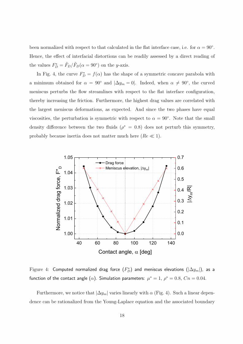
been normalized with respect to that calculated in the flat interface case, i.e. for α = 90◦.
Hence, the effect of interfacial distortions can be readily assessed by a direct reading of
the values F ∗D = FD/FD(α = 90◦) on the y-axis.
In Fig. 4, the curve F ∗D = f(α) has the shape of a symmetric concave parabola with
a minimum obtained for α = 90◦ and |∆ym = 0|. Indeed, when α = 90◦, the curved
meniscus perturbs the flow streamlines with respect to the flat interface configuration,
thereby increasing the friction. Furthermore, the highest drag values are correlated with
the largest meniscus deformations, as expected. And since the two phases have equal
viscosities, the perturbation is symmetric with respect to α = 90◦. Note that the small
density difference between the two fluids (ρ∗ = 0.8) does not perturb this symmetry,
probably because inertia does not matter much here (Re ≪ 1).
40 60 80 100 120 140
1.00
1.01
1.02
1.03
1.04
1.05 Drag force Meniscus elevation, |Dym|
Contact angle, a [deg]
Nor
mal
ized
dra
g fo
rce,
F* D
0.0
0.1
0.2
0.3
0.4
0.5
0.6
0.7
|Dy m
/R|
Figure 4: Computed normalized drag force (F ∗D) and meniscus elevations (|∆ym|), as a
function of the contact angle (α). Simulation parameters: µ∗ = 1, ρ∗ = 0.8, Cn = 0.04.
Furthermore, we notice that |∆ym| varies linearly with α (Fig. 4). Such a linear depen-
dence can be rationalized from the Young-Laplace equation and the associated boundary
18

conditions governing the meniscus shape around the floating cylinder. The details of the
derivation are presented in the appendix. With the notations of Fig. 9 (cf. appendix), it
can be shown that
|∆ym| = 2Lc sin
(α− β
2
), (23)
where β is the floating angle (Fig. 9). Within the explored range of α values, it turns out
that the argument (α− β)/2 remains small and does not exceed 7.5◦. Therefore, to first
order, |∆ym| ≈ Lc(α− β), which explains the linearity of |∆ym| vs. α in Fig. 4.
Figs. 5a,b display typical velocity fields calculated for α = 110◦. When compared to
Fig. 2b (α = 90◦), the influence of the meniscus is clearly reflected by a deformed flow
pattern. The PF map of Fig. 5c shows the interfacial deformations in the neighborhood
of the cylinder. The corresponding mesh, superimposed on the PF map, is exhibited
on Fig. 5d, which shows that the fluid interface is well-resolved within the subdomains,
according to the criterion defined earlier (Sec. 4).
Overall, the data of Fig. 4 show that, for µ∗ = 1, the effect of interfacial deformations
on F ∗D is rather moderate within the probed range of α, yielding an excess drag, defined
as (F ∗D−1)×100 (in %), on the order of 5% compared to the case of a flat interface. Note
that this order of magnitude compares well with that obtained by Danov et al. [9], who
computed 3D excess drag coefficients for an infinite, flat, and nonviscous fluid interface
with µ∗ = 1. By shifting the particle up and down across the undistorted interface, which
amounts to testing several contact angles, the authors report a similar concave shape for
the curve fd = f(α) with fd [cf. Eq. (1)] ranging up to 1.05. Hence, similarly to the
curved meniscus, shifting the particle’s vertical position breaks the symmetry of the flow
pattern and results in an increased drag.
Experimentally, only a few studies considered the hydrodynamical behavior of particles
trapped at fluid interfaces with matched viscosities (typically, oil-water systems). For
instance, Vassileva et al. [21] and Boneva et al. [22, 23] tracked the trajectories of pairs of
interacting sub-millimeter spheres and deduced an excess drag coefficient of around 10−
20%, presumably ascribed to interfacial deformations. However, one should bear in mind
that actual colloidal systems at fluid interfaces are far from “ideal” and feature a lot more
19
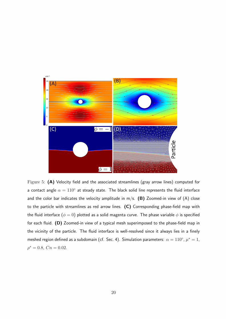
Figure 5: (A) Velocity field and the associated streamlines (gray arrow lines) computed for
a contact angle α = 110◦ at steady state. The black solid line represents the fluid interface
and the color bar indicates the velocity amplitude in m/s. (B) Zoomed-in view of (A) close
to the particle with streamlines as red arrow lines. (C) Corresponding phase-field map with
the fluid interface (ϕ = 0) plotted as a solid magenta curve. The phase variable ϕ is specified
for each fluid. (D) Zoomed-in view of a typical mesh superimposed to the phase-field map in
the vicinity of the particle. The fluid interface is well-resolved since it always lies in a finely
meshed region defined as a subdomain (cf. Sec. 4). Simulation parameters: α = 110◦, µ∗ = 1,
ρ∗ = 0.8, Cn = 0.02.
20

complications. For instance, the particle surface roughness, chemical inhomogeneities,
contact angle hysteresis or the ubiquitous presence of a variety of contaminants are only
but a few of the phenomena which are likely to profoundly alter the response of the system
and dash the hope of an easy comparison with idealized computations.
Hence, with the above proviso in mind, both simulations and experiments qualitatively
agree on the fact that a deformed fluid interface, with matched viscosities, enhances only
slightly the drag force on the particle.
6.2 Influence of the viscosity ratio
In this section, we examine how a viscosity difference between the two fluids affects the
drag force. We will consider a two-order-of-magnitude change of µ∗ in the range 0.01− 1,
by altering the upper fluid viscosity (µ1) whilst keeping that of the lower one (µ2) constant
(see table 1). The particle is held fixed at the center of the box (yp = 0).
First, only a slight deviation of µ∗ from unity is investigated as a function of the
contact angle. With µ∗ = 0.75, we see that the curve F ∗D = f(α) reported on Fig. 6 is no
longer symmetric with respect to α = 90◦. Its minimum is shifted towards larger α and
is now reached for α = 100◦. Furthermore, the highest drag force is obtained for α < 90◦,
i.e. when the meniscus is convex and deformed upwards. Indeed, when α decreases, the
size of the region underneath the meniscus grows as the meniscus becomes more and more
distorted. This leads to an enhanced friction since the lower fluid is more viscous than the
upper one. Equivalently, for µ∗ > 1, the minimum drag would have been shifted towards
α < 90◦ and the highest drag force would have occurred for α > 90◦. Furthermore,
because of the small capillary number, note that the values of |∆ym| do not depend on
µ∗ and, consequently, they are the same here as those reported in Fig. 4.
Thus, for µ∗ = 1, our results show that one can encounter situations where the flat
interface case (α = 90◦) actually causes more friction than a slightly non-flat one. This
finding departs from the common belief that interfacial disturbances yield necessarily an
extra hydrodynamic resistance.
Note that, for µ∗ = 1, the drag force exerted on the particle should normally be
21

40 60 80 100 120 1400.99
1.00
1.01
1.02
1.03
1.04
1.05
1.06 µ*=1 µ*=0.75
Nor
mal
ized
dra
g fo
rce,
F* D
Contact angle, a [deg]
Figure 6: Computed normalized drag force (F ∗D) as a function of the contact angle (α) for two
viscosity ratios (µ∗). For µ∗ = 0.75, the curve is no longer symmetric with respect to α = 90◦
and the minimum drag force is obtained for a slightly non-flat interface with α = 100◦. See
text for further details. Simulation parameters: ρ∗ = 0.8, Cn = 0.04.
22
accompanied by a non-zero viscous torque as well. The main reason for this is that, with
fluids of different viscosity, the drag force’s line of action does not generally run through
the particle’s center of mass, as first mentioned by Dorr & Hardt [24]. Consequently, the
particle is expected to rotate in this case. Actually, particle rotation is also expected to
occur even for µ∗ = 1 as long as there is an up-down asymmetry in the flow pattern.
The latter may be caused either by interfacial distortions, as we saw in Sec. 6.1, or
simply by shifting the particle position across an otherwise flat interface [9]. Anyway, as
aforesaid (end of Sec. 3.2), we have ignored such a rotation in the present study, where the
particle is kept fixed with respect to the passing flow. Allowing particle rotation implies
that the contact line dynamics would have to be taken into account. Although the PF
method is well-adapted to tackle such an issue [25, 30, 39, 40], we will leave it for a future
investigation.
We also performed simulations with much larger viscosity mismatches, i.e. much
smaller values of µ∗. The graph of Fig. 7a represents dimensional drag force values
plotted vs. µ∗ for three different contact angles (75◦, 90◦, and 110◦). The data obtained
for α = 90◦ serve as a reference with a flat fluid interface. Since inertia is negligible
(Re ≪ 1), the drag force follows the expected linear dependence on µ∗ for the three α’s.
Next, we note that the data points for α = 110◦ mostly lie below those computed for
α = 90◦, especially at low values of µ∗. Upon re-plotting these data using normalized
drag forces (Fig. 7b), we see more clearly that F ∗D(α = 110◦) falls well below unity as µ∗
decreases, while the opposite trend is observed for F ∗D(α = 75◦). This result is a further
evidence that the presence of interfacial deformations can actually yield a state of lower
drag when compared to its undisturbed counterpart. Furthermore, recall that the particle
position is the same for all these data and that the meniscus profiles do not depend on
µ∗. Therefore, for either α = 75◦ or α = 110◦, it is not too surprising to see that the
shift of F ∗D with respect to unity grows as the viscosity mismatch is further increased.
Coming back to Fig. 6, it means that both the curve asymmetry, with respect to α = 90◦,
and the well depth, with respect to unity, would be enhanced for much lower values of
µ∗. This statement suggests that the larger the viscosity mismatch, the larger the drag
23
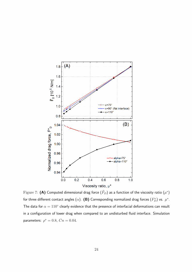
Figure 7: (A) Computed dimensional drag force (FD) as a function of the viscosity ratio (µ∗)
for three different contact angles (α). (B) Corresponding normalized drag forces (F ∗D) vs. µ
∗.
The data for α = 110◦ clearly evidence that the presence of interfacial deformations can result
in a configuration of lower drag when compared to an undisturbed fluid interface. Simulation
parameters: ρ∗ = 0.8, Cn = 0.04.
24
enhancement or reduction. For instance, the maximum excess drag force in Fig. 6 does
increase from ≃ 4.5% for µ∗ = 1 to ≃ 6% for µ∗ = 0.75. The use of smaller viscosity
ratios, such as µ∗ = 0.02, actually makes the maximum excess drag go above 10% for
α = 45◦ and ρ∗ = 0.8 (data not shown). An equally important drag reduction occurs for
α = 135◦ in this case.
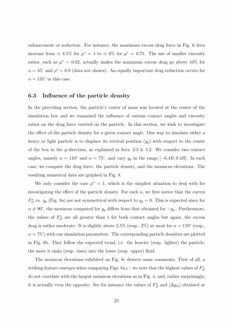
6.3 Influence of the particle density
In the preceding section, the particle’s center of mass was located at the center of the
simulation box and we examined the influence of various contact angles and viscosity
ratios on the drag force exerted on the particle. In this section, we wish to investigate
the effect of the particle density for a given contact angle. One way to simulate either a
heavy or light particle is to displace its vertical position (yp) with respect to the center
of the box in the y-direction, as explained in Secs. 3.3 & 5.2. We consider two contact
angles, namely α = 110◦ and α = 75◦, and vary yp in the range [−0.4R, 0.4R]. In each
case, we compute the drag force, the particle density, and the meniscus elevations. The
resulting numerical data are graphed in Fig. 8.
We only consider the case µ∗ = 1, which is the simplest situation to deal with for
investigating the effect of the particle density. For each α, we first notice that the curves
F ∗D vs. yp (Fig. 8a) are not symmetrical with respect to yp = 0. This is expected since for
α = 90◦, the meniscus computed for yp differs from that obtained for −yp . Furthermore,
the values of F ∗D are all greater than 1 for both contact angles but again, the excess
drag is rather moderate. It is slightly above 2.5% (resp., 2%) at most for α = 110◦ (resp.,
α = 75◦) with our simulation parameters. The corresponding particle densities are plotted
in Fig. 8b. They follow the expected trend, i.e. the heavier (resp. lighter) the particle,
the more it sinks (resp. rises) into the lower (resp. upper) fluid.
The meniscus elevations exhibited on Fig. 8c deserve some comments. First of all, a
striking feature emerges when comparing Figs. 8a,c : we note that the highest values of F ∗D
do not correlate with the largest meniscus elevations as in Fig. 4, and, rather surprisingly,
it is actually even the opposite. See for instance the values of F ∗D and |∆ym| obtained at
25
Figure 8: (A) Computed normalized drag force (F ∗D) as a function of the particle position
across the interface (yp) for two different contact angles (α). (B) Corresponding particle
densities (ρp) calculated from the interfacial profiles as explained in Secs. 3.3 & 5. (C)
Associated meniscus elevations (|∆ym|). The black arrows mark a change in the meniscus
curvature, which is illustrated by the two zoomed-in phase-field snapshots at the bottom.
Simulation parameters: µ∗ = 1, ρ∗ = 0.8, Cn = 0.04.
26
yp = ±0.3R on Figs. 8a,c. Therefore, for a given contact angle, it seems like the amount of
drag is primarily controlled by the particle position across the interface, and not only by
the interfacial distortions. Otherwise stated, the same value of |∆ym| may well correspond
to two different values of F ∗D depending on yp . And this is indeed well-illustrated for e.g.
α = 75◦, where |∆ym| is about the same for both yp = −0.1R and yp = −0.4R, but the
corresponding drag forces differ significantly (Fig. 8a).
Next, we note that the minimum drag in Fig. 8a is obtained for small particle dis-
placements (yp ≃ ±0.1R) and moderate |∆ym| (< 0.2R). Further increasing |yp| always
results in an enhanced drag force, even if |∆ym| drops substantially. One might argue
that the increase in F ∗D for large values of |yp| is the result of a confinement effect, i.e. one
of the walls being a bit closer to the particle surface. However, using single-phase flow
simulations (Sec. 5), we checked that confinement effects manifest themselves only when
the particle surface is typically less than one diameter away from the moving wall. In all
the configurations considered in Fig. 8, yp ranges from −0.4R to 0.4R and the separation
distance between the cylinder surface and the walls always exceeds several diameters.
Consequently, one may rule out any influence of the confining walls on the drag force
values when the particle is moved across the fluid interface.
Finally, the solid arrows on Fig. 8c mark the cases where the meniscus curvature
changes sign. More precisely, for those values of yp , the otherwise concave (resp. con-
vex) meniscus normally obtained for α = 110◦ (resp. α = 75◦) cannot be retained and
it gradually becomes flat and then convex (resp. concave). The curvature reversal is
illustrated by the two zoomed-in phase-field snapshots at the bottom of the graph. This
‘meniscus transition’ goes in pairs with a new increase in |∆ym| and is responsible for the
non-monotonic variation of |∆ym| vs. yp (Fig. 8c).
7 Concluding remarks
The primary goal of the present study was to explore, through 2D numerical simulations,
the influence of interfacial distortions on the drag force exerted on a particle straddling
a fluid interface. We mainly focused on the effects of three parameters, the contact
27

angle, the viscosity ratio, and the particle density. For fluids of equal viscosity and the
particle centered on the initially flat interface, our results reveal that the drag force is an
increasing function of interfacial deformations with the minimum drag obtained with a
flat interface. Introducing a viscosity difference between the two fluids alters this intuitive
picture as a state of lower drag may actually be achieved with a non-flat interface rather
than with a flat one. Furthermore, high viscosity mismatches seem to favor either large
drag enhancement or large drag reduction depending on the contact angle.
Other counter-intuitive findings are found when tuning the particle density. In this
case, with matched fluid viscosities, we have shown that the drag force is again not
necessarily an increasing function of interfacial deformations. Indeed, “high” drag config-
urations are possible even with small meniscus distortions depending on how the particle
is positioned across the interface. This result has never been predicted nor experimentally
evidenced before. Thus, based on the above findings, two main interesting insights emerge:
(i) large drag forces may not always correspond to large interfacial distortions, and (ii),
the drag force is strongly affected by the location of the particle across the interface.
Another salient result is that interfacial deformations do not seem to yield significant
drag variations compared to the case of a flat interface. As an upper bound order of
magnitude, our simulation data indicate that interfacial distortions may increase or de-
crease the drag coefficient by about 10% within the explored physical parameters. This
result is the first simulated estimate of the influence of fluid interface perturbations on
the mobility of interfacial particles. It is consistent with drag enhancement observed
in experiments involving liquid-liquid interfaces [21, 22, 23] but larger differences exist
with data compiled from experiments performed at liquid-gas interfaces [14]. However,
in the latter case, the physical parameters greatly differ from those we used in our study.
Nevertheless, let us recall here that a painstaking comparison between simulations and
experiments was beyond the scope of the present work, whose primary objective was to
capture qualitative trends through an approximate 2D approach.
Overall, our study unearthed unexpected findings on a rather simple situation where
the interfacial deformations were caused by the buoyant weight of macroscopic particles.
28

While this situation applies down to length scales, say, ≈ 50µm, it is worth pointing out
that interfacial distortions also exist when dealing with much smaller adsorbed particles.
In this case, gravity is no longer relevant but the particle’ surface roughness, the chemical
inhomogeneities, the presence of surface electric charges or the nonspherical shape all serve
as other potential sources of interfacial perturbations, possibly with undulating contact
lines as well [2, 4, 41]. How do these phenomena impact drag forces? Such issues pertain to
a much broader class of colloidal systems, including biological membranes, and definitely
warrant more in-depth investigations. We hope that the present study will foster the
development of other simulations or theoretical calculations on the topic we have touched
upon herein.
Acknowledgements
This work was financially supported by the EU Marie-Curie fellowship ‘CoPEC’ under
grant No 794837–H2020-MSCA-IF-2017 and by the NSERC Discovery grant No 2019-
04162. One of us (J.-C.L.) is also indebted to the University of Bordeaux for further
financial support thanks to the IdEx program entitled “Developpement des carrieres -
Volet personnel de recherche”. M.Q. wishes to thank for the support of the four-year
Doctoral Fellowship of the University of British Columbia. The IT staff of the Mathe-
matics department of the University of British Columbia is also gratefully acknowledged
for their valuable help and support.
Author contributions
J.-C.L. and J.J.F. designed research; J.-C.L. and M.Q. performed research; all authors
analyzed the data, interpreted the results and collaborated on the manuscript.
Appendix: Derivation of Eq. (23)
The details for deriving Eq. (23) in Sec. 6.1 can be found in [38]. Here, we summarize
29

the main steps of the calculations.
Figure 9: Geometry of the floating circular cylinder used to derive Eq. (23) in the appendix.
The fluid interface is defined by the function y(x). Definitions of symbols: R, cylinder radius;
α, contact angle; β, floating angle; θ, interface slope; ∆ym, meniscus elevation.
With the notations of Fig. 9, we consider a static situation where a circular cylinder
floats at a fluid interface, which is described by the function y(x). We set the origin of
the y-axis at the position of the flat interface far from the particle. Since the interface
curvature, noted as κ, also tends to zero far from the particle, the hydrostatic Young-
Laplace equation governing the shape of the 2D curved fluid interface in our problem is
written as
κ = − y
L2c
, (24)
where Lc is the capillary length introduced in Sec. 3.2. The curvature is given by
κ = − y′′
(1 + y′2)3/2=
1
y′
(1√
1 + y′2
)′
=1
y′d| cos θ|
dx, (25)
where y′ = dy/dx = tan θ, as shown in Fig. 9, with the prime denoting a derivative
with respect to x. Combining Eq. (24) with the last two expressions of Eq. (25) and
rearranging, we obtain the following nonlinear differential equation for the fluid interface:
d
dx
(1√
1 + y′2
)=
d| cos θ|dx
= −yy′
L2c
= −(y2)′
2L2c
.
30

Integrating once with respect to x, we get
1√1 + y′2
= | cos θ| = − y2
2L2c
+ C , (26)
where C is a dimensionless integration constant. Requiring that both y and θ decay to
zero as x tends to infinity, we obtain C = 1. At the contact line, we have θcl = α − β
and ycl = ∆ym (see Fig. 9), so that the last two expressions of Eq. (26) give
(∆ym)2
2L2c
= 1− cos(α− β) = 2 sin2
(α− β
2
), (27)
where the absolute value has been dropped since the angle (α−β) is always smaller than
π/2. Finally, Eq. (27) yields Eq. (23)
|∆ym| = 2Lc sin
(α− β
2
).
References
[1] Kralchevsky PA, Nagayama K (2000) Capillary interactions between particles bound
to interfaces, liquid films and biomembranes. Adv. Coll. Interf. Sci. 85:145-192.
[2] Danov KD, Kralchevsky PA (2010) Capillary forces between particles at a liquid
interface: General theoretical approach and interactions between capillary multipoles.
Adv. Coll. Interf. Sci. 154:91-103.
[3] McGorty R, Fung J, Kaz D, Manoharan VN (2010) Colloidal self-assembly at an
interface. Materials Today 13(6):34-42.
[4] Dasgupta S, Aust T, Gompper G (2017) Nano- and microparticles at fluid and bio-
logical interfaces. J. Phys.: Condens. Matter 29(37):373003 (41pp).
[5] Du K, Liddle JA, Berglund AJ (2012) Three-dimensional real-time tracking of
nanoparticles at an oilwater interface Langmuir 28:9181-9188.
31
[6] O’Neill ME, Ranger KB, Brenner H (1986) Slip at the surface of a translatingrotating
sphere bisected by a free surface bounding a semiinfinite viscous fluid: Removal of
the contact line singularity. Phys. Fluids 29(4):913-924, and references therein.
[7] Brenner H, Leal LG (1978) A micromechanical derivation of Fick’s law for interfacial
diffusion of surfactant molecules. J. Colloid Interface Sci. 65(2):191-209.
[8] Danov KD, Aust R, Durst F, Lange U (1995) Influence of the surface viscosity on
the hydrodynamic resistance and surface diffusivity of a large Brownian particle. J.
Colloid Interface Sci. 175:36-45.
[9] Danov KD, Dimova R, Pouligny B (2000) Viscous drag of a solid sphere straddling
a spherical or flat interface. Physics of Fluids 12:2711-2722.
[10] Pozrikidis C (2007) Particle motion near and inside an interface. J. Fluid Mech.
575:333-357.
[11] Ally J, Amirfazli A (2010) Magnetophoretic measurement of the drag force on
partially immersed microparticles at airliquid interfaces. Colloids and Surfaces A:
Physicochem. Eng. Aspects 360:120-128.
[12] Dani A, Keiser G, Yeganeh M, Maldarelli C (2015) Hydrodynamics of particles at
an oil-water interface. Langmuir 31:13290-13302.
[13] Dorr A, Hardt S, Masoud H, Stone HA (2016) Drag and diffusion coefficients of a
spherical particle attached to a fluid interface. J. Fluid. Mech. 790:607-618.
[14] Petkov JT, Denkov ND, Velev OV, Danov KD, Aust R, Durst F (1995) Measurement
of the drag coefficient of spherical particles attached to fluid interfaces. J. Colloid
Interface Sci. 172:147-154.
[15] Petkov JT, Danov KD, Denkov ND, Aust R, Durst F (1996) Precise method for
measuring the shear surface viscosity of surfactant monolayers. Langmuir 12:2650-
2653.
32

[16] Dimova R, Danov KD, Pouligny B, Ivanov IB (2000) Drag of a solid particle trapped
in a thin film or at an interface: Influence of surface viscosity and elasticity. J. Colloid
Interface Sci. 226:35-43.
[17] Fischer TM, Dhar P, Heinig P (2006) The viscous drag of spheres and filaments
moving in membranes or monolayers. J. Fluid Mech. 558:451-475.
[18] Boniello G, Blanc C, Fedorenko D, Medfai M, Mbarek NB, In M, Gross M, Stocco
A, Nobili M (2015) The viscous drag of spheres and filaments moving in membranes
or monolayers. Nat. Mater. 14:908-913.
[19] Koplik J, Maldarelli C (2017) Diffusivity and hydrodynamic drag of nanoparticles at
a vapor-liquid interface. Phys. Rev. Fluids 2:024303-1–12.
[20] Das S, Koplik J, Farinato R, Nagaraj DR, Maldarelli C, Somasundaran P (2018)
The translational and rotational dynamics of a colloid moving along the air-liquid
interface of a thin film. Scientific Reports 8:8910-1–13.
[21] Vassileva ND, van den Ende D, Mugele F, Mellema J (2005) Capillary forces between
spherical particles floating at a liquid-liquid interface. Langmuir 21:11190-11200.
[22] Boneva MP, Christov NC, Danov KD, Kralchevsky PA (2007) Effect of electric-field
induced capillary attraction on the motion of particles at an oil-water interface. Phys.
Chem. Chem. Phys. 9:6371-6384.
[23] Boneva MP, Danov KD, Christov NC, Kralchevsky PA (2009) Attraction between
particles at a liquid interface due to the interplay of gravity- and electric-field-induced
interfacial deformations. Langmuir 25(16):9129-9139.
[24] Dorr A, Hardt S (2015) Driven particles at fluid interfaces acting as capillary dipoles.
J. Fluid. Mech. 770:5-26.
[25] Worner M (2012) Numerical modeling of multiphase flows in microfluidics and micro
process engineering: a review of methods and applications. Microfluid Nanofluid
12:841-886.
33

[26] Jacqmin D (1999) Calculation of two-phase NavierStokes flows using phase-field mod-
eling. J. Comput. Phys. 155:96-127.
[27] Yue P, Feng JJ, Liu C, Shen J (2004) A diffuse-interface method for simulating
two-phase flows of complex fluids. J. Fluid Mech. 515:293-317.
[28] Pigeonneau F, Hachem E, Saramito P (2019) Discontinuous Galerkin finite element
method applied to the coupled unsteady Stokes/Cahn-Hilliard equations. Int. J. Nu-
mer. Meth. Fluids 90:267-295.
[29] Yue P, Zhou C, Feng JJ, Ollivier-Gooch CF, Hu HH (2006) Phase-field simulations of
interfacial dynamics in viscoelastic fluids using finite elements with adaptive meshing.
J. Comput. Phys. 219:47-67.
[30] Yue P, Zhou C, Feng JJ (2010) Sharp-interface limit of the Cahn-Hilliard model for
moving contact lines. J. Fluid Mech. 645:279-294.
[31] COMSOL Multiphysicsr version 5.4 reference manual. See https://www.comsol.
com/documentation.
[32] Guyon E, Hulin JP, Petit L, Mitescu CD (2015) Physical Hydrodynamics (Oxford
University Press 2nd Ed.).
[33] Khalili A, Liu, B (2017) Stokes’ paradox: creeping flow past a two-dimensional cylin-
der in an infinite medium. J. Fluid Mech. 817:374-387.
[34] Faxen OH (1946) Forces exerted on a rigid cylinder in a viscous fluid between two
parallel fixed planes. Proc. R. Swed. Acad. Eng. Sci. 187:1-13.
[35] Ben Richou A, Ambari A, Lebey M, Naciri JK (2005) Drag force on a circular cylinder
midway between two parallel plates at Re ≪ 1 Part 2: moving uniformly (numerical
and experimental). Chem. Eng. Sci. 60:2535-2543.
[36] See chapter 18 of the COMSOL Multiphysicsr reference manual [31] for details on
deformed geometries and moving meshes.
34
[37] The analytical expressions derived in [38] for the vertical force balance of a cylinder
floating at a fluid interface are only valid in an unbounded geometry. Due to the finite
size of the simulation box, we should therefore expect differences in the computed
interfacial profiles when comparing the results. However, it turns out that these
differences are very small, at most barely noticeable as mentioned in Sec. 5.2 (cf.
Fig. 3). We believe that the box length, L ≃ 6Lc (cf. Table 1), is long enough so
that confinement effects have a minimum impact on the meniscus shape.
[38] Pozrikidis C (2017) Fluid Dynamics. Theory, Computation, and Numerical Simula-
tion (Springer 3rd Ed., New York). See chapter 5.
[39] Seppecher P (1996) Moving contact lines in the Cahn-Hilliard theory. Int. J. Engng.
Sci. 34(9):977-992.
[40] Jacqmin D (2000) Contact-line dynamics of a diffuse fluid interface. J. Fluid Mech.
402:57-88.
[41] Botto L, Lewandowski EP, Cavallaro M Jr, Stebe KJ (2012) Capillary interactions
between anisotropic particles. Soft Matter 8:9957-9971.
35