draft september 8, 2010web.williams.edu/economics/wp/montielremittancesandtherealexcha… · the...

1

DRAFT September 8, 2010

Workers’ Remittances and the Equilibrium Real Exchange Rate: Theory and Evidence

Adolfo Barajas, Ralph Chami, Dalia Hakura, and Peter Montiel*

Abstract

This paper investigates the impact of workers’ remittances on equilibrium real exchange rates (ERER) in recipient economies. Using a small open economy model, it shows that standard “Dutch Disease” results of appreciation are substantially weakened or even overturned depending on: degree of openness, factor mobility between domestic sectors, and countercyclicality of remittances; the share of consumption in tradables; and the sensitivity of a country’s risk premium to remittance flows. Panel cointegration techniques on a large set of countries provide support for these analytical results, and show that ERER appreciation in response to sustained remittance flows tends to be quantitatively small.

JEL Classification Numbers: F24, F31 Keywords: Remittances, Real Exchange Rate, Dutch Disease

* Barajas, Chami, and Hakura are at the International Monetary Fund. Montiel is at Williams College.

3

International economic integration in the early 21st century is conventionally thought of in

terms of increased openness to trade in goods and services, as well as a dramatic increase in the

volume of capital flows. The 21st century experience is sometimes contrasted with that of the last

wave of globalization at the end of the 19th century, when increased integration on both of those

dimensions was also accompanied by large waves of international migration. However, this

contrast is probably overdrawn, as increases in international flows of labor services have also

been characteristic of the current wave of globalization, and the impact of these factor movements

is increasingly making itself felt in the international economy.

A particularly dramatic manifestation of this fact is the sharp recorded increase in flows of

worker remittances to the large number of developing countries that have been the source of these

flows of labor services. In recent years, many such countries have witnessed significant increases

in remittance flows, to the point that their scale has come to dwarf that of other types of resource

inflows, whether development assistance, foreign direct investment, or other types of capital

flows. In 2007, remittance flows to Sub-Saharan Africa were equal in magnitude to flows of

official development assistance, for example. Remittance flows now account for some 17 percent

of GDP and 77 percent of exports in El Salvador, and over 20 percent of GDP and nearly 50

percent of exports in Honduras. In these countries, remittance flows are more than five times

larger than FDI flows.

Unlike capital flows, remittances do not entail the creation of external debt with future

4

repayment obligations; unlike foreign development assistance, they do not come encumbered with

a variety of political and economic conditions with which the recipient country must comply.

Despite these virtues, however, large inflows of worker remittances have been perceived as

posing macroeconomic challenges for the recipient countries.1 One specific challenge is that

large inflows of worker remittances could lead to the emergence of “Dutch disease. That is,

remittance inflows could result in an appreciation of the equilibrium real exchange rate that would

tend to undermine the international competitiveness of domestic production, particularly that of

nontraditional exports.

Accordingly, the purpose of this paper is to analyze the effect of worker remittances on

the equilibrium real exchange rate in recipient countries. Our specific concerns are to investigate

analytically the conditions under which an increase in worker remittances would indeed tend to

appreciate the equilibrium real exchange rate, and to bring some empirical evidence to bear on

this issue. For the analytical component our strategy is to use a simple “workhorse” model of a

small open economy to derive the standard result that an increase in remittance inflows results in

an equilibrium real appreciation, and then investigate the conditions under which this conclusion

could be reversed.2 Our main conclusion is that the “benchmark” case in which a permanent

increase in the flow of worker remittances results in an appreciation of the long-run equilibrium

real exchange rate comparable to that which would result from a similar permanent increase in the

receipt of exogenous international transfers is a rather special one: reasonable modifications in the

modeling of the factors driving remittances, or in the various macroeconomic roles that

1 For an overview, see Chami et. al. (2008). 2 We will apply a model previously used in Montiel (1999) to explore the determinants of the equilibrium real exchange rate.

5

remittances may play, could moderate or even reverse the expected impact of remittance flows on

the equilibrium value of the real exchange rate. The implication is that the presumption that a

permanent increase in workers’ remittances causes an appreciation in the long-run equilibrium

real exchange rate is too facile: the complicated macroeconomic roles that remittances play in

recipient economies allow for a multiplicity of possible outcomes, and the issue is therefore an

empirical one. We investigate this issue empirically by applying panel cointegration techniques,

employing the largest set of countries for which remittance data are available. After controlling

for a large number of fundamental determinants of the equilibrium real exchange rate we find that

despite the theoretical ambiguities, the empirical evidence is indeed consistent with an

appreciation of the equilibrium real exchange rate in response to a sustained inflow of workers’

remittances, but the empirical effects that we find are quantitatively very small. The implication

is that the presence of substantial remittance inflows need not necessarily pose a challenge to an

export-oriented development strategy.

The paper is organized as follows. The next section provides an overview of the scale of

the remittance phenomenon. Section II describes the analytical framework, derives the standard

result within that framework, and considers how differences both in the factors driving

remittances as well as in the impact of remittances on other macroeconomic variables may affect

the equilibrium value of the real exchange rate. Section III reviews previous empirical work on

the effects of remittances on the equilibrium real exchange rate, based both on individual country

studies as well as on panel data. Our own panel estimates are presented in Section IV. The final

section summarizes and concludes. Appendix A provides a formal analysis of the model

described in Section II, while Appendix B provides a list of the countries used in our empirical

6

work.

I. How important are remittance flows?

Flows of workers’ remittances appear to have been increasing sharply in magnitude during

recent years. While related impressionistic evidence suggests that most of this increase is real, it

is not possible to assess its magnitude conclusively, because part of the increase in recorded flows

may simply reflect improved recording systems. Nevertheless, taking available data at face value,

remittance inflows averaged over 4 percent of GDP for a group of 128 countries that have

remittance data over the past decade (1998-2007), compared to 3.7 percent over the entire 1970-

2007 period, and by 2007 they had increased to over 5 percent of GDP (Table 1). Figure 1

documents that, while remittance inflows had been on an increasing trend since the early 1970s,

they increased particularly sharply in the aggregate over the past decade.

1970 - 2007 1998 - 2007 2007

Mean workers' remittances-to-GDP ratio across

countries and time 3.7 4.2 5.1

Maximum workers' remittances-to-GDP ratio across

countries and time 45.4 45.4 45.4

Number of countries 128 118 110

Number of observations 2,235 988 110

Cross-country standard deviation 5.0 5.7 7.7

Source: World Bank WDI Database, International Monetary Fund WEO Database, and authors'

calculations.

Table 1. Developing Countries: Workers' Remittances (in percent of GDP)

7

Table 2 compares the size of remittance inflows with that of other foreign exchange flows

for developing countries. As shown in the table, remittance inflows dwarf official transfers,

official capital flows, and non-FDI private capital inflows. Their importance as a source of

foreign exchange is also demonstrated by the fact that, in the aggregate, they amount to some 30

percent of the total exports of developing countries.

0

500

1000

1500

2000

0.0

50.0

100.0

150.0

200.0

250.0

1970 1975 1980 1985 1990 1995 2000 2005

Figure 1. Worldwide Workers' Remittances, 1970-2007

World workers' remittances (billions of US dollars, left scale)

Workers' remittances per country (millions of US dollars, right scale)

8

There is a substantial amount of variation across regions as well as across individual

developing countries in the magnitude of remittance receipts. As shown in Figure 2, remittance

receipts are much larger in Asia and Latin America than in Africa, Central and Eastern Europe,

and the CIS countries, largely because of the large flows received by economies such as India and

Mexico. The largest remittance recipients scaled by GDP are shown in Figure 3. While by this

measure the largest recipients tend to be small economies with large diasporas, large countries

such as Nigeria and Bangladesh also receive remittance inflows that are in excess of 10 percent of

GDP.

Table 2. Developing Countries: Workers' Remittances in Relation to Selected Balance of Payments

Inflows

Ratio of Workers' Remittances to

Official

Transfers

Official

Capital

Flows

Private

Capital

Flows

Exports

Recent period, 1998-2007

Mean across countries and time 14.8 18.3 2.4 0.3

Maximum country average 289.2 810.1 38.8 4.4

Cross-country standard deviation 42.3 89.0 5.6 0.6

Recent observation: 2007

Mean 19.2 9.6 2.4 0.3

Maximum 186.2 142.8 52.8 7.2

Cross-country standard deviation 35.7 21.7 8.1 0.9

Sources: World Bank WDI Database, International Monetary Fund WEO Database, and authors'

calculations.

9

II. Effects of remittances on the equilibrium real exchange rate: theory

In this section we will investigate the implications of standard theory for the effects of

worker remittance flows on the recipient economy’s equilibrium real exchange rate, and will

consider how these implications would be affected by simple modifications to the standard

framework. The model underlying the analysis of this section is described formally in an

0.0

10.0

20.0

30.0

40.0

50.0

60.0

70.0

1980 1982 1984 1986 1988 1990 1992 1994 1996 1998 2000 2002 2004 2006

(bill

ions of U

.S. dolla

rs)

Figure 2. Workers' Remittances by Region: Developing Countries, 1980-2007

Africa Central and Eastern Europe

Common Wealth of Independent States Developing Asia

Middle East Western Hemisphere

0.0

5.0

10.0

15.0

20.0

25.0

30.0

35.0

40.0

45.0

50.0

Taj

ikis

tan

Tonga

Guya

na

Hondura

s

Leb

anon

Mold

ova

Kyr

gyz

Hai

ti

El S

alvad

or

Jord

an

Nep

al

Jam

aica

Nic

arag

ua

Bos.

& H

erz.

Ser

bia

Guat

emal

a

Alb

ania

Nig

eria

Sen

egal

Ban

gla

des

h

(in p

erce

nt

of

GD

P)

Figure 3. Top 20 Recipient Countries: Ratio of Workers' Remittances to GDP, 2007

10

appendix, which also derives the results described below.

1. Analytical framework

To examine the effects of remittance inflows on the equilibrium real exchange rate, we

consider a small open economy with a fixed nominal exchange rate and flexible domestic wages

and prices.3 The economy has a two-sector “dependent economy” production structure, with

traded and nontraded goods production sectors. A fixed labor force moves freely between the two

sectors. In this setting, the supply of traded goods depends directly, and that of nontraded goods

inversely, on the real exchange rate e, measured as the relative price of traded goods in terms of

nontraded goods.

Nontraded goods are purchased by the household sector as well as the government.

Household demand for nontraded goods increases with total real household consumption c

(measured in units of traded goods) as well as with depreciation of the real exchange rate (which

makes nontraded goods relatively cheaper).4 We take the government’s demand for nontraded

goods to be exogenous. Since an increase in total household consumption expenditure increases

the demand for nontraded goods, maintaining equilibrium in the market for nontraded goods,

which we refer to as “internal balance,” requires a real exchange rate appreciation, which

simultaneously increases the supply of nontraded goods and reduces the demand for them. This

relationship is depicted graphically as the locus IB (for internal balance) in Figure 4. For the

3 The assumption of flexible domestic wages and prices is an innocuous one, since any meaningful definition of the equilibrium real exchange imposes full employment. 4 We assume a unitary elasticity of substitution in consumption between traded and nontraded goods.

11

reasons mentioned above, this locus must have a negative slope.

Figure 4 Determination of the equilibrium real exchange rate

The equilibrium real exchange rate is that which is simultaneously consistent with internal

as well as external balance, where the latter is defined as a current account deficit/surplus equal to

the “sustainable” value of capital inflows/outflows. We define the latter as the rate of capital

inflow (or outflow) required to sustain the value of the economy’s real international investment

position at its steady-state level. In turn, the steady-state value of the economy’s international

investment position is determined as follows: we assume that the economy is financially open,

and faces a risk premium in international financial markets that is a decreasing function of the

economy’s real international investment position (which has the implication that more indebted

economies face higher risk premia). This real external cost of funds determines the domestic real

interest rate in steady state. For the economy to attain a steady-state equilibrium, that real interest

rate must equal the exogenously-given household rate of time preference, so that household

e

IB

EB

c

c*

e*A

12

consumption is neither increasing nor decreasing over time. Thus the steady-state value of the

international investment position is that which produces a risk premium that equates the

economy’s real interest rate to the rate of time preference.5 The sustainable value of capital flows

is the product of the steady-state value of the economy’s international investment position and an

exogenous world inflation rate.

The current account balance is the sum of the trade balance, remittance inflows, and the

interest payments/receipts associated with the country’s international investment position. The

latter is the product of the nominal interest rate on external debt/assets (given by the rate of time

preference plus the world inflation rate, both of which are exogenous) and the steady-state

international investment position. The trade balance, in turn, is the difference between domestic

output of traded goods, which is an increasing function of the real exchange rate, and the sum of

household and government demand for such goods. Household demand is proportional to

household consumption expenditure c, with the factor of proportionality equal to the weight of

traded goods consumption in the household’s utility function plus transactions costs per unit of

real consumption. The latter are used to motivate the holding of money in the model, and are

arbitrarily assumed to be incurred in the form of traded goods (but see the discussion of this issue

below). We take government demand for traded goods to be exogenous. In this setup, an increase

in steady-state real household consumption requires a real exchange rate depreciation, which

maintains external balance by shifting domestic production to traded goods. This implies that the

external balance locus must have a positive slope in Figure 4.

5 Note the implication is that more ‘impatient” economies will be larger steady-state net debtors.

13

The equilibrium real exchange rate is defined by the intersection of the internal and

external balance loci at point A in Figure 4, and is labeled e*. Note that the steady-state value of

household consumption is determined simultaneously with that of the real exchange rate.

With this analytical framework in hand, we can now examine how the equilibrium real

exchange rate responds to a change in remittance inflows, which affects the positions of the IB

and EB curves. We will consider several cases. The first two cases focus on the factors driving

remittances, while the last two consider how the effects of remittances on the equilibrium value of

the real exchange rate are altered if remittances have other macroeconomic effects - specifically,

if they affect the risk premium faced by the recipient country and if they enter household utility

functions directly.

2. Exogenous remittances

Consider first the standard case, in which remittances are treated as exogenous inflows,

similar to the receipt of foreign grants. Remittance receipts represent an addition to household

incomes equal to the amount of remittances. As such, they appear as an additive term in the

economy’s aggregate budget constraint, given by its external balance condition.6 Accordingly,

the effect of a permanent increase in the receipt of remittances is to shift the external balance

locus to the right -- an increase in remittance flows allows a higher level of household

consumption to be consistent with external balance at an unchanged value of the real exchange

6 In terms of the formal model in the appendix, remittances enter as an additive term in the household budget constraint (6), in the dynamic equation (21) for a, and in the steady-state equilibrium condition (28).

14

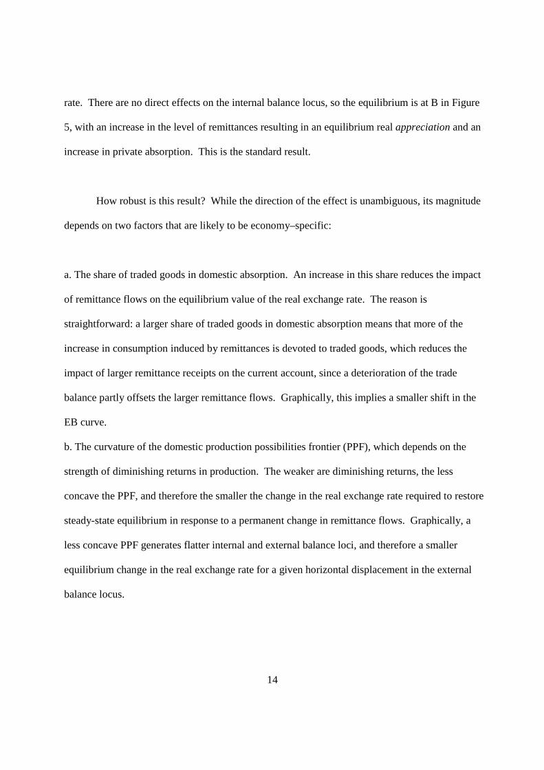
rate. There are no direct effects on the internal balance locus, so the equilibrium is at B in Figure

5, with an increase in the level of remittances resulting in an equilibrium real appreciation and an

increase in private absorption. This is the standard result.

How robust is this result? While the direction of the effect is unambiguous, its magnitude

depends on two factors that are likely to be economy–specific:

a. The share of traded goods in domestic absorption. An increase in this share reduces the impact

of remittance flows on the equilibrium value of the real exchange rate. The reason is

straightforward: a larger share of traded goods in domestic absorption means that more of the

increase in consumption induced by remittances is devoted to traded goods, which reduces the

impact of larger remittance receipts on the current account, since a deterioration of the trade

balance partly offsets the larger remittance flows. Graphically, this implies a smaller shift in the

EB curve.

b. The curvature of the domestic production possibilities frontier (PPF), which depends on the

strength of diminishing returns in production. The weaker are diminishing returns, the less

concave the PPF, and therefore the smaller the change in the real exchange rate required to restore

steady-state equilibrium in response to a permanent change in remittance flows. Graphically, a

less concave PPF generates flatter internal and external balance loci, and therefore a smaller

equilibrium change in the real exchange rate for a given horizontal displacement in the external

balance locus.

15

In short, we would expect more open economies, economies with more flexible labor

markets, and economies in which the traded goods sector is intensive in factors that are also used

in the production of nontraded goods (e.g., unskilled or semi-skilled labor) to display a smaller

response of the equilibrium real exchange rate to a change in remittance flows. This being said,

however, these factors affect only the quantitative response of the equilibrium real exchange rate.

Qualitatively, our analysis up to this point is consistent with the conventional view that an

increase in remittance flows should be associated with an appreciation of the equilibrium real

exchange rate.

Figure 5. Effects of an increase in remittances on the equilibrium real exchange rate

e

IB

EB

c

c*

e*A

EB’

B

16

3. Induced remittances

We now explore how this conclusion may be affected by modifications in the model. The

most drastic simplifying assumption in the analysis above is that remittances simply represent an

exogenous income flow. An alternative model of remittances would view them as responsive to

domestic household incomes – i.e., family members working abroad remit to the domestic

economy when their relatives who have remained behind are experiencing low household

incomes, and are less generous when domestic household incomes are high.

To see how this more realistic description of remittance behavior would affect the model,

suppose that remittance inflows consist of two components: an autonomous component and a

component that is a decreasing function of domestic real income, measured in units of traded

goods. Under this assumption, total remittance inflows become endogenous in the external

balance condition. Because a real exchange rate depreciation reduces domestic real income (by

reducing the traded-good value of nontraded goods production), it would tend to increase the

level of remittances. The implication is that the dependence of remittances on household income

strengthens the effect of the real exchange rate on the current account, because it simultaneously

increases output of traded goods and increases the level of remittances. Graphically, the slope of

the EB curve becomes flatter. Since the slope of the IB curve is unaffected, the implication is that

a change in autonomous component of remittances that would have the same impact on the

horizontal position of the EB curve as in the case in which remittances are exogenous would now

have a weaker effect on the equilibrium real exchange rate. The reason is that autonomous

17

changes in remittances will give rise to real exchange rate changes that are opposite in sign to

those of the change in autonomous remittances, and thus to changes in real income that are of the

same sign as the change in autonomous remittances (i.e., remittances and real income will be

positively correlated), which in turn will induce a reversal in remittance flows.

In short, allowing for induced remittances in this fashion weakens, but does not reverse,

the conventional view about the effect of remittance flows on the equilibrium real exchange rate.

4. Effects operating through the risk premium

In the two cases analyzed previously, workers’ remittances affected the recipient economy

only through their direct effects on national income. In practice, however, the channels through

which remittances influence the recipient economy may be more complicated, and as we will now

show, these additional channels may alter the qualitative effects of remittances on the equilibrium

real exchange rate.

Going back to the case of exogenous remittances, note that for changes in exogenous

remittances to affect the steady-state equilibrium real exchange rate, these changes must be

permanent. But if a country experiences a permanent change in remittance receipts, the

capitalized value of those receipts represents a change in its national wealth and thus should affect

the risk premium that it faces in international capital markets, just as would a resource discovery

or a long-lasting improvement in the country’s terms of trade. The IMF, for example, has found

empirical evidence that changes in remittance flows have significant effects on country credit

18

ratings (see IMF 2005).

To capture this channel, assume that the risk premium faced by the domestic economy

depends on its international investment position plus the capitalized value of its “permanent”

remittance inflows. To see how this modification affects the previous result note that, since the

steady-state risk premium is determined by the domestic rate of time preference and the world

real interest rate, it cannot be affected by changes in remittance flows in the steady state.

Consequently, the “remittance-inclusive” value of national wealth must be unaffected in steady-

state equilibrium by a permanent change in the value of remittance flows: such a change must be

offset by a change in the country’s international investment position. This surprising result has a

simple interpretation: on impact, a permanent increase, say, in the size of remittance inflows gives

rise to an increase in domestic absorption in the same direction. But contrary to what happens

when the country’s borrowing costs are assumed to be unaffected by remittance receipts, in this

case the reduction in the country risk premium induces a temporary increase in absorption that

actually exceeds the increase in the value of remittance flows, causing the country’s net

international investment position to decrease over time until it exactly offsets the change in the

capitalized value of remittance flows, leaving the remittance-inclusive stock of national wealth

unaffected in steady state.

The implications for the equilibrium real exchange rate are important. As in the previous

subsection, the internal balance condition is unchanged. Moreover, it is easy to see that a change

in the permanent value of remittances has no effect on the external balance locus under the

19

assumption that the risk premium depends on the capitalized value of the remittance stream. The

reason is that, since an increase in remittance inflows must reduce the economy’s international

investment position by an amount equal to the present value of the increased inflows, it must

reduce the country’s steady-state interest income by exactly the amount of the increase in

remittance inflows. The positive impact of an increase in remittance flows on the current account

is therefore exactly offset by a reduced flow of interest income due to a deterioration in the

country’s steady-state net investment position. The implication is that an increase in remittance

flows has no effect on the EB locus, and thus leaves the long-run equilibrium real exchange rate

unchanged.

The upshot is that the conventional presumption that increases in workers’ remittances

causes the equilibrium real exchange rate to appreciate no longer holds when the effects of

remittance flows on country risk premia are taken into account.

5. Effects operating through household utility functions

Up to this point, the analysis has assumed that remittance receipts are like any other form

of income, in that they affect the resources available to households and therefore the level of

household spending, but have no effect on household preferences over the composition of

consumption. It is possible, however, that the receipt of remittances could affect household

preferences. If so, the effect of remittance receipts on the long-run equilibrium real exchange rate

would also be affected.

20

To take an extreme case, suppose that households devote all remittance income to the

purchase of traded goods. For this to be the case, remittances must not be regarded by households

in the aggregate as simply another source of income, but must directly influence how the

representative consumer values different types of goods.7 We can capture this in our analytical

framework by assuming that the utility that the household derives from the consumption of traded

goods depends on the excess of such consumption over the value of remittances. This has the

effect of increasing the marginal utility of traded goods consumption, at a given value of such

consumption, by a greater amount the larger the flow of remittance receipts. In this case, as shown

in the appendix, the household will devote all of its remittance receipts to consuming traded

goods, and then divide any additional consumption between traded and nontraded goods just as

before. The upshot is that, for a given total level of household consumption, an increase in

remittance receipts increases consumption of traded goods more than before, at the expense of

consumption of nontraded goods.

The implications for the behavior of the internal and external balance conditions are clear.

Since an increase in remittance receipts results in a smaller improvement in the current account at

a given value of the real exchange rate than before (due to the offsetting effect of the increase in

consumption of tradables), the rightward shift in the EB locus must be smaller than before. At the

same time, because the increase in remittance receipts decreases consumption demand for

nontradables (at any given value of total real consumption c), the internal balance locus IB must

7For this effect to be present, it is not necessary that an increase in remittance receipts, say, changes a specific household’s utility function. It may simply be the case that household who receive remittances have a stronger preference for traded goods, and an increase in remittance receipts increases the share of aggregate consumption attributable to such households.

21

shift to the right in this case (because the depressed demand for nontradables means that an

increase in total consumption is required to keep the market for nontraded goods in equilibrium).

Both effects serve to weaken the effect of the change in remittances on the equilibrium real

exchange rate.

Could the sign of the effect be reversed? Consider first the case in which transactions

costs associated with consumption are negligible – i.e., suppose the economy being described is a

nonmonetary one.8 In this case it is easy to see that an increase in remittance inflows that is

exactly offset by an increase in household consumption c would continue to satisfy the internal

and external balance conditions. In the case of the internal balance condition, the reason is that

this combination of changes would leave consumption of nontraded goods unchanged. In the case

of the external balance condition, it is because an increase in consumption that exactly matches

the increase in remittances would mean that consumption of traded goods would increase by

exactly the same amount as the increase in remittances, leaving the current account unchanged.

This means that a permanent increase in remittances must give rise to an increase in household

spending of exactly the same amount, all of which is devoted to traded goods. Since the internal

and external balance conditions would continue to be satisfied in this situation, the long-run

equilibrium real exchange rate would be unchanged – that is, the change in the size of remittance

receipts would have no effect on the long-run equilibrium real exchange rate. Graphically, under

these circumstances an increase in remittances would simply shift the internal and external

balance loci to the right by exactly the same amounts, increasing the equilibrium level of

8 If transactions costs are zero, there is no incentive for holding money in this economy.

22

consumption by that amount, but leaving the equilibrium value of the real exchange rate

unchanged.

Now consider the more general case in which transactions costs are nonzero. If

transaction costs are borne in the form of traded goods, then an increase in consumption

expenditure exactly equal to the increase in remittances would increase domestic absorption of

traded goods by more than the increase in remittance flows, because of the additional absorption

of traded goods into transactions costs. To retain external balance, therefore, the increase in c

would have to be smaller than that in remittance flows. The upshot is that the EB curve would

shift rightward by less than the increase in remittance flows, and therefore by less than the IB

curve (which would not be affected by the introduction of transactions costs in this case),

resulting in a depreciation in the long-run equilibrium real exchange rate. 9 The key point is that

the effect of a permanent increase in remittance inflows on the long-run equilibrium real exchange

rate becomes indeterminate for a monetary economy when remittance receipts are fully spent on

traded goods.10

We conclude that, while theory may indeed suggest a strong presumption in favor of the

9 Alternatively, if transactions costs are borne primarily in the form of nontraded goods, this situation would be reversed: the IB curve would shift to the right by less than the EB curve, and the long-run equilibrium real exchange rate would appreciate once again. 10 What if they are fully spent on nontraded goods (e.g., education or construction) instead? The analysis is not symmetric. In this case, a given level of real consumption would be reoriented toward nontraded goods. In the absence of transactions costs, an increase in consumption equal to the increase in remittances, but devoted solely to the purchase of nontraded goods, would cause the EB locus to shift to the right, since the positive effect of remittances on the current account would not be offset by higher consumption of traded goods. However, the IB locus would shift to the left, because the increased spending on nontradables would create an excess demand for such goods at the original value of the real exchange rate, requiring a downward adjust in consumption expenditures. The upshot is that the equilibrium value of the real exchange rate would have to appreciate. Allowing for transactions costs modifies these results in the same way as before.

23

conventional view associating an increase in remittance inflows with an appreciation of the

equilibrium real exchange rate, there are various conditions under which this association may be

weak, others in which there may be no association at all, and finally some in which the

conventional view may even be reversed. The effect of changes in worker remittance flows is

therefore an empirical issue.

III. Remittances and the equilibrium real exchange rate: evidence

Empirical work on this issue is surprisingly scarce, especially in light of the voluminous

literature that now exists on the estimation of equilibrium real exchange rates. Yet despite the

large role that remittance receipts play in many developing countries and their growing

importance, the literature on estimation of equilibrium real exchange rate has not typically

incorporated remittance flows into the set of real exchange rate fundamentals.

Existing work on this issue has examined both individual country experience as well as

cross- country evidence. The standard approach in individual country studies is to include

remittance flows in the set of fundamentals that enter a cointegrating equation for the real

exchange rate, together with other potential real exchange rate determinants.

An early single-country study of this type was by Bourdet and Falck (2003). They

examined the effect of workers’ remittances on the equilibrium real exchange rate in Cape Verde

over the period 1980-2000 and confirmed the conventional view that an increase in remittance

receipts is associated with an appreciation of the equilibrium real exchange rate. Similar results

24

were derived by Hyder and Mahboob (2005) for Pakistan during 1978-2005, as well as Saadi-

Sedik and Petri (2006) for Jordan over 1964-2005.

By contrast, Izquierdo and Montiel (2006) found mixed results for six Central American

countries over the period 1960-2004. In the cases of Honduras, Jamaica, and Nicaragua, they

found no influence of workers’ remittances on the equilibrium real exchange rate, despite the fact

that these countries received very large remittance inflows over the last half of their sample. On

the other hand, remittance inflows turned out to affect the equilibrium real exchange rate in the

conventional direction in the Dominican Republic, El Salvador, and Guatemala. However,

remittances had a significantly stronger effect on the equilibrium real exchange rate in El

Salvador and Guatemala than in the Dominican Republic.

Given the small set of countries examined to date in single-country studies to date, it is

difficult to generalize from these results. However, other researchers have used panel methods to

examine the effects of remittance inflows on the real exchange rate in larger groups of countries.

An early study was by Amuedo-Dorantes and Pozo (2004). They used a panel with 13

Latin American and Caribbean countries, estimating with data drawn from the period 1978-98,

and found support for the conventional view – i.e., an increase in worker remittances was

associated with an appreciation of the real exchange rate in their sample. Subsequent research has

greatly expanded the country sample. Both Holzner (2006) as well as Lopez, Molina, and

Bussolo (2007) found similar qualitative result using much larger samples of countries drawn

25

from several regions, although the quantitative impact of remittance flows on the real exchange

rate found by Lopez et al were much smaller than those of Amuedo-Dorantes and Pozo. More

recently, Lartey, Mandelman and Acosta (2008), as well as Acosta, Baerg and Mandelman (2009)

derived similar results for a much larger sample of countries (both papers used an unbalanced

panel of 109 developing and transition economies with data from 1990 to 2003). However, the

results of these studies turned out to be subject to some qualifications. For example, Acosta,

Baerg and Mandelman found that the effect of remittance inflows on the real exchange rate

tended to decrease as the degree of financial development increased. They also found that there

was no significant effect of remittances on the real exchange rate in countries with British legal

origins.

Moreover, the support for the conventional view has not been universal. Rajan and

Subramanian (2005) found, for a sample of 15 countries and data from the decade of the 1990s,

that higher remittance receipts were not associated with slower growth either in manufacturing

industries that had higher labor intensity or those with a greater export orientation, as one might

expect if remittance receipts are associated with Dutch disease effects operating through an

appreciated real exchange rate.

It is particularly important to note that none of the panel studies described above

specifically tests for the presence of a common stochastic trend among the real exchange rate and

its fundamentals by applying a cointegration methodology. Instead, they essentially examine the

contemporaneous effect of changes in worker remittances on the actual real exchange rate. As

such, the effects that they estimate may be purely transitory ones, which leave the equilibrium real

26

exchange rate unchanged. The effects of permanent changes in remittance flows on the

equilibrium real exchange rate therefore remain unexamined.

IV. Panel evidence

The upshot is that neither the single-country nor panel evidence speaks with a single

voice. While most of the research to date is indeed consistent with the conventional presumption

that larger remittance receipts tend to appreciate the equilibrium real exchange rate, the verdict is

not unanimous on this issue. We thus turn to our own panel estimation, using a large set of

countries as well as more recent data and a more complete set of real exchange rate fundamentals

than those employed in earlier studies. Most importantly, however, because the real exchange rate

proves to be nonstationary in almost all countries, and indeed proved to be nonstationary in our

panel unit root tests (see Table 3 below), unlike the existing panel literature we focus specifically

on the identification of common stochastic trends among the real exchange rate and its

fundamental determinants, including worker remittance flows. As a result, we are able to

estimate the effects of sustained changes in such flows on the equilibrium, rather than just the

actual, real exchange rate.

The first step in applying our panel cointegration methodology is to identify the full set of

fundamentals that may affect the equilibrium real exchange rate in addition to the flow of worker

remittances. Unfortunately, theory suggests a large number of potential fundamentals, and while

many studies that estimate the equilibrium real exchange rate using cointegration methods tend to

restrict themselves to a small subset of the potential fundamentals (often without justifying the ex

27

ante exclusion of others), we can only be confident of our results if we can rule out that

remittance flows are in fact proxying for some relevant, but excluded, fundamental. For that

purpose, we have sought to include the most comprehensive set of theoretically-suggested

fundamentals for which data are available. Fortunately, a recent study by Christiansen et al

(2009) on the determinants of external balance in low-income countries compiled data on a large

set of potential real exchange rate fundamentals for a comprehensive sample of countries. The

availability of their dataset allows us to include a relatively large group of countries as well as a

large number of potential fundamentals.11 The dataset includes 138 countries, consisting of 56

upper-middle- and high-income countries, 38 lower-middle income countries and 44 low-income

ones (following the World Bank country classification, as described in the Data Appendix). We

have expanded their set of fundamentals by including flows of worker remittances scaled by

GDP, which was not one of the fundamentals considered in their study. Unfortunately, this

variable is not available for all of the countries in their study, and our sample is therefore different

from theirs. Because of the availability of the data for all of the fundamentals, the largest number

of countries included our regression estimations is 79 for the all countries sample, 16 for the low

income countries sample, and 31 for the low- and lower-middle income countries sample.

11 The data were made available through the IMF internal web site.

28

The dependent variable in all of our estimated cointegrating equations is the log of the

effective (trade-weighted) real exchange rate (REER).12 Our set of fundamentals, in addition to

the ratio of workers’ remittances to GDP (denoted WREC in the tables below), includes official

aid as a percentage of GDP, each country’s net international investment position (NFA, using the

net present value of debt in the case of low-income countries with largely concessional debt)

relative to GDP, its real per capita GDP (in logs), the country’s fertility rate as a proxy for its age-

dependency ratio, the terms of trade, the ratio of government consumption to GDP, indexes of

trade and capital account restrictions (both separately as well as in the form of the black market

premium, which may capture both trade and capital account restrictions13), indicators of the

prevalence of administered agricultural prices as well of the severity of agricultural price

intervention, and a variable measuring the incidence of natural disasters. The theoretical rationale

for the inclusion of each of these variables, and their expected signs in the cointegrating

equations, are provided in Christiansen et al (2009). The last three variables in this list are

somewhat unconventional, but because they are potentially important in explaining variations in

the real exchange rate for low-income countries in particular, and because such countries are

heavily overrepresented among remittance recipients, we retain them here. The sources for the

non-remittance data are described in Christiansen et al (2009), and the remittance data are taken

from the World Bank’s Word Development Indicators (WDI).

12 Contrary to our convention in the analytical model, the real exchange rate in our empirical estimation is expressed as the relative price of home goods in terms of foreign goods, so an increase indicates a real appreciation. The real effective exchange rate (REER) index is the nominal effective exchange rate index adjusted for relative changes in consumer prices, obtained from the IMF’s Information Notice System database. An alternative approach would have been to construct a REER measure using national price levels from the Penn World Tables, but Christiansen et al found nearly identical results with the two measures. 13 Note that both the trade and capital account restriction variables are measured in such a way that an increase denotes lower restrictions, that is, greater openness.

29

We estimate the cointegrating equation between the real effective exchange rate and the

set of fundamentals described above using an unbalanced panel of annual data for the 1980-2007

period. Our estimation method is dynamic least squares (DOLS) with fixed effects and one lead

and one lag of the changes in each fundamental. With the exception of the natural disaster, black

market premium, and capital account liberalization variables, panel unit root tests confirm that all

of the variables have unit roots (Table 3).14 Three sets of results are reported below for the

coefficients of the cointegrating vector: one for the full sample of countries (Table 4), one for

low-income countries (Table 5), and one for low and lower-middle-income countries (Table 6).

In each table, eight different results are reported: columns (1) – (4) use the values of the

explanatory variables in levels, with columns (5) – (8) measuring the explanatory variables as

deviations from their trade-weighted partner-country counterparts, following Christiansen et al

(2009).15 The reason for doing so is as follows: conceptually, we would like to measure the real

exchange rate as the relative price of traded in terms of nontraded goods (as in our analytical

model), sometimes referred to as the “internal” real exchange rate (see Hinkle and Montiel 1999).

To detect the effects of the fundamentals – including that of remittance flows – on the internal

real exchange rate, deviations from trading partner values in the explanatory variables would not

be relevant, since the internal real exchange rate responds only to home-country values of the

fundamentals, as in our model. In practice, however, measures of the internal real exchange rate

are not widely available, and most studies of equilibrium real exchange rates (including our own)

14 In contrast to the other fundamental variables reported, the fertility and trade restrictions variables are expressed relative to the trade-weighted average of trading partners, because they are only available in that form in the Christiansen et al data set. 15 Group mean ADF panel cointegration tests for the regressions reported in columns 3 and 7 respectively of Table 4 reject the null hypothesis of no cointegration.

30

therefore use CPI-based measures of the effective real exchange rate. Under these circumstances,

it may be important to take account of potential changes in the relative price of traded in terms of

nontraded goods among each country’s trading partners. Expressing the explanatory variables as

deviations from partner-country variables allows this to be done, because under this approach a

country’s real effective exchange rate will change in response to a change in a fundamental only if

that fundamental changes more or less in the home country than in its trading partners, implying a

larger or smaller impact on the relative price of traded goods in the home country than in its

trading partners. This correction is less important if changes in the CPI-based real exchange rate

are empirically dominated by changes in the domestic relative price of traded goods, rather than

that of the country’s trading partners. Since this is difficult to ascertain ex ante, we include both

sets of results.

31

Column (1) in Table 4 reports our results for all countries with all potential fundamentals

included (except the black market premium: see below) in the estimated cointegrating equation.

Most of the non-remittance fundamentals have the theoretically-predicted signs and are

statistically significant at least at the 95 percent confidence level.16 The sign of the coefficient of

the ratio of workers’ remittances to GDP, however, is inconsistent with the conventional view that

a sustained increase in such flows results in an appreciation of the equilibrium real exchange rate

16 Note that the ratio of aid to GDP, which is virtually always negatively signed and statistically signifcant, has a strong influence on the performance of non-remittance fundamentals. When excluding the aid variable, all non-remittance variables are correctly signed and significant at least at the 95 percent confidence level. However, it does not appear to have a strong effect on the sign or significance of workers’ remittances.

Variable Statistic P-value

Log of Real Eeffective Exchange Rate -0.333 0.37

Workers' remittances to GDP (WREC) 5.53 1.00

Net foreign assets to GDP 2.012 0.98

Relative productivity (log) 3.917 1.00

Real per capita GDP 6.642 1.00

Terms of trade good (log) -0.261 0.40

Government consumption to GDP-deviation 2.292 0.99

Government consumption to GDP 0.559 0.71

Aid to GDP Ratio 11.469 1.00

Aid to GDP Ratio-deviations 5.646 1.00

Capital account liberalization-deviation -5.007 0.00

Capital account liberalization -4.075 0.00

Trade restrictions-deviation 3.303 1.00

Administered agricutural prices-deviation 38.605 1.00

Administered agriultural prices 1.377 0.92

Maximum agricultural price intervention - deviation 7.141 1.00

Maximum agricultural price intervention 32.355 1.00

Fertility-deviation 1.492 0.93

Natural disaster -3.085 0.00

Black market premium -1.844 0.03

1 Based on Pesaran (2007). The null hypothesis assumes that all series are non-

stationary. The test is conducted for the all countries sample and is restricted to

having at least 10 uninterrupted time observations per country.

Table 3. Panel Unit Root Test statistics1

32

(which would require the coefficient to be positive). Excluding the somewhat ad hoc “natural

disasters” variable, as in column (2), does not materially affect the results.

Column (3) expands the country sample by excluding several variables (NFA, the

productivity ratio, the index of trade restrictions, and the index of administered agricultural

prices) that have limited data. While the magnitudes and statistical significance of the remaining

(1) (2) (3) (4) (5) (6) (7) (8)

Workers' remittances to GDP (WREC) -0.00550 -0.0054 0.0100* 0.0231*** 0.0002 0.0005 0.0118** 0.0200***

(-0.9599) (-0.9502) (1.9283) (3.0550) (0.0275) (0.0874) (2.4517) (2.7530)

Aid to GDP -4.023*** -4.0163*** -2.9594*** -1.2600*** -1.2058** -1.2101** -1.2023*** -1.0090**

(-5.2588) (-5.2344) (-4.4485) (-2.8555) (-2.0297) (-2.0390) (-4.0132) (-2.2875)

Net foreign assets 0.0231* 0.0243* 0.0231* 0.0243*

(1.820) (1.8934) (1.8174) (1.8934)

Government Consumption to GDP 2.118*** 2.1194*** 2.6520*** 1.7536*** 1.6621*** 1.6698*** 1.9609*** 1.3179*

(4.7702) (4.7629) (5.2637) (2.7350) (3.4318) (3.4367) (4.2055) (1.9196)

Terms of trade goods (log) 0.117** 0.1184** 0.1744*** 0.1875** 0.1657*** 0.1709*** 0.2100*** 0.1872**

(2.4947) (2.5267) (3.4537) (2.2680) (3.3043) (3.3750) (4.0552) (2.2216)

Fertility (in deviations) 0.109*** 0.1091*** 0.1218*** 0.1603*** 0.1177*** 0.1269*** 0.1276*** 0.1732***

(4.0370) (4.1052) (5.3831) (4.8803) (5.0347) (5.4497) (5.9899) (5.5094)

Real GDP per capita -0.168*** -0.1693*** -0.1506* -0.1421*

(-3.5897) (-3.6312) (-1.9417) (-1.8300)

Index of capital account liberalization (CAP100) 0.0300 0.0279 -0.0439 0.0728 0.0734 0.0604 0.1469** 0.1874**

(0.4702) (0.4442) (-0.6951) (0.9014) (1.0188) (0.8393) (2.3736) (2.1940)

Trade restrictions ( in deviations) -0.175** -0.1737** 0.2617*** 0.2450***

(-2.4544) (-2.4571) (3.2326) (3.0252)

Administered agricultural prices -0.0926* -0.0935* -0.1253** -0.1315**

(-1.8121) (-1.8318) (-2.3198) (-2.4372)

Maximum agricultural price intervention -0.0168 -0.0169 0.0192 0.0036 -0.0490 -0.0496 -0.0009 0.0121

(-0.4158) (-0.4188) (0.5126) (0.0671) (-1.1626) (-1.1818) (-0.0229) (0.2270)

Natural disaster -0.00686 -0.0793***

(-0.2495) (-2.9144)

Black market premium (%) 0.2114*** 0.2271***

(2.8834) (3.0373)

Constant 5.540*** 5.5385*** 3.3573*** 2.8594*** 3.9734*** 3.8670*** 3.5743*** 3.1655***

(10.8415) (10.8552) (13.4990) (6.8868) (15.6904) (15.4212) (14.5100) (7.0411)

Observations 1,234 1,234 1,285 657 1,042 1,042 1,178 634

R-squared 0.691 0.69 0.62 0.79 0.70 0.70 0.65 0.79

Only countries with at least ten years of uninterrupted yearly observations are included. t-statistics in parentheses; significance levels

of 10% (*), 5%(**), and 1% (***) indicated.

Table 4. Panel Cointegration Results, All Countries

Regressions in levels Regressions in deviations

This table reports the results of Dynamic Ordinary Least Squares regressions of the logarithm of the real effective exchange rate on a set of

fundamentals, including the ratio of workers' remittances to GDP (WREC). Columns (1) - (4) show the results for regressions using all explanatory

variables in levels, while columns (5) - (8) show the results of regressions in which the following variables are expressed as deviations with respect

to trading partners: Aid to GDP, Fertility, Government Consumption to GDP, CAP100, Real PPP GDP per capita, Trade restrictions, Maximum

agricultural price intervention, and Administered agricultural prices.

33

fundamentals are not greatly affected by this change, the effect of worker remittances on the

equilibrium real exchange rate is now conventionally signed and is statistically significant.

Notice, however, that the effect is not economically very significant. The reported coefficient for

workers’ remittances can be interpreted as a semi-elasticity. The results in column (3) suggest

that a one percentage-point increase in the remittance ratio (roughly a 20 percent change in the

scale of remittance flows relative to the average among all developing countries in 2007) would

result in an equilibrium real appreciation of about one-hundredth of one percent. When the black

market premium is included as an alternative indicator of real and financial distortions in cross-

border trade (column 4) this effect increases in magnitude, but remains very small, at 0.023

percent.

As mentioned above, it is possible that these results are contaminated by changes in the

relative price of traded goods in each country’s trading partners, as the result of using the CPI-

based real effective exchange rate, rather than the “internal” real exchange rate. To explore that

possibility, we repeat the empirical exercise with explanatory variables now expressed as ratios to

the same variables in each country’s trade-weighted trading partners. The results are reported in

columns (5) – (8). They are very similar to those of columns (1) – (4).17 For our purposes, the

key result is that remittance flows continue to be statistically insignificant when the full set of

fundamentals is included. With the restricted set of fundamentals, the remittance variable again

displays the conventionally-expected sign and is statistically significant, but its estimated impact

on the equilibrium real exchange rate remains very small.

17 One difference, however, is that the trade restrictions variable changes sign. We do not yet have an explanation for this.

34

The macroeconomic role of remittance flows may be quite different in industrial countries

and in middle-income developing countries from what it is in low-income countries. Industrial

countries are largely the sources of remittance flows rather than their destinations, and the size of

such flows tends to be much smaller in such countries relative to the size of their economies.

Middle-income countries tend on the one hand to be larger than low-income countries, and

therefore less open on average, while on the other hand they are more likely to depend on private

capital flows – and thus to be affected by the effects of remittances on sovereign risk premia –

than are low-income ones. Our analytical model suggests that these two characteristics should

affect the impact of remittances on the real exchange rate in opposite directions, with the former

strengthening the impact and the latter weakening it. Moreover, the size of remittance flows tends

to be systematically smaller – whatever their sign –relative to the size of their economies in

industrial and middle-income countries. The relevance of the country sample is confirmed in

Tables 5 and 6, which report the result of restricting the sample only to low-income countries, or

to low- and lower-middle-income countries, respectively.

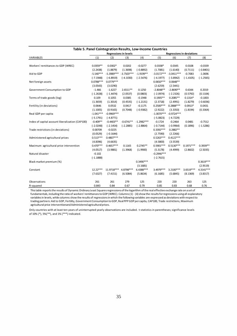
35

VARIABLES (1) (2) (3) (4) (5) (6) (7) (8)

Workers' remittances to GDP (WREC) 0.0359** 0.0302* 0.0202 -0.0277 0.0338* 0.0345 0.0108 -0.0339

(2.2438) (1.8879) (1.3698) (-0.8892) (1.7081) (1.6140) (0.7111) (-0.8401)

Aid to GDP -5.540*** -5.3989*** -3.7503*** -1.9199** -3.0172*** -3.0411*** -0.7083 -1.0696

(-7.1948) (-6.8919) (-4.1030) (-2.5476) (-4.1977) (-3.8942) (-1.4105) (-1.2565)

Net foreign assets 0.0788*** 0.0779*** 0.0650*** 0.0648**

(3.0543) (3.0290) (2.6259) (2.5441)

Government Consumption to GDP -1.466 -1.6227 2.6511** 0.1250 -2.8048** -2.8690** 0.6344 0.2019

(-1.2638) (-1.4474) (2.0537) (0.0803) (-2.0974) (-2.2326) (0.5792) (0.1104)

Terms of trade goods (log) 0.109 0.1055 0.0385 -0.1948 0.1905** 0.2085** 0.1314* -0.1003

(1.3659) (1.3014) (0.4535) (-1.2131) (2.3718) (2.4991) (1.8279) (-0.6036)

Fertility (in deviations) 0.0646 0.0532 0.0417 -0.1175 0.2500*** 0.2888*** 0.0913* 0.0431

(1.1005) (0.9165) (0.7048) (-0.9382) (2.9222) (3.3350) (1.8194) (0.3364)

Real GDP per capita -1.041*** -0.9969*** -1.0070*** -0.9724***

(-5.1791) (-4.8771) (-5.0823) (-4.7229)

Index of capital account liberalization (CAP100) -0.409** -0.4403** -0.6741** -1.2982*** -0.1724 -0.2464 0.0481 -0.7512

(-2.0248) (-2.1454) (-2.2885) (-2.8864) (-0.7144) (-0.9964) (0.1896) (-1.5286)

Trade restrictions (in deviations) 0.00709 -0.0225 0.3392*** 0.2882**

(0.0529) (-0.1644) (2.7590) (2.2266)

Administered agricultural prices 0.513*** 0.4807*** 0.5263*** 0.4122***

(4.8396) (4.6635) (4.5800) (3.5539)

Maximum agricultural price intervention 0.470*** 0.4657*** 0.1165 0.2745** 0.5901*** 0.5130*** 0.1971*** 0.3939**

(4.0517) (3.9881) (1.3968) (1.9900) (5.3178) (4.4999) (2.8602) (2.5035)

Natural disaster -0.102 -0.2946***

(-1.1888) (-2.7615)


(3.1685) (2.9519)

Constant 12.22*** 11.9718*** 4.8798*** 6.4388*** 3.4979*** 3.2100*** 3.6519*** 4.3141***

(7.6327) (7.4151) (6.5084) (5.8634) (6.1685) (5.6845) (8.1369) (3.8317)

Observations 261 261 279 125 220 220 263 125

R-squared 0.843 0.84 0.67 0.79 0.85 0.83 0.68 0.76


of 10% (*), 5%(**), and 1% (***) indicated.

Table 5. Panel Cointegration Results, Low-Income Countries




variables in levels, while columns show the results of regressions in which the following variables are expressed as deviations with respect to

trading partners: Aid to GDP, Fertility, Government Consumption to GDP, Real PPP GDP per capita, CAP100, Trade restrictions, Maximum

agricultural price interventionand Administered agricultural prices.

36

The results become somewhat stronger when the sample is extended to lower-middle-

income countries as well, thereby encompassing a more complete sample of remittance-receiving

countries. The significance increases noticeably for certain non-remittance fundamentals, such as

government consumption, terms of trade, and agricultural price intervention. For workers’

remittances in particular, the coefficient is now correctly signed in all regressions, and is

VARIABLES (1) (2) (3) (4) (5) (6) (7) (8)

Workers' remittances to GDP (WREC) 0.0108 0.0105 0.0173*** 0.0322*** 0.0167** 0.0170** 0.0172*** 0.0298***

(1.5407) (1.4992) (2.7193) (3.5653) (2.2194) (2.2995) (2.7758) (3.2646)

Aid to GDP -4.377*** -4.4421*** -3.2043*** -1.1595** -1.3474** -1.3597** -1.3146*** -1.1148**

(-5.7974) (-5.7758) (-4.4230) (-2.4874) (-2.2218) (-2.2476) (-4.1642) (-2.4408)

Net foreign assets 0.0209 0.0205 0.0028 0.0033

(1.4718) (1.4400) (0.2119) (0.2499)

Government Consumption to GDP 2.531*** 2.6256*** 3.5913*** 2.2216*** 1.9835*** 1.9003** 2.6976*** 2.0516***

(3.4671) (3.6307) (4.8231) (3.1028) (2.6148) (2.5092) (4.4948) (2.6879)

Terms of trade goods (log) 0.134** 0.1368** 0.1851*** 0.2743*** 0.1643** 0.1641** 0.2090*** 0.2585**

(2.1753) (2.2573) (3.0360) (2.6447) (2.5655) (2.5691) (3.3865) (2.4240)

Fertility (in deviations) 0.148*** 0.1421*** 0.1289*** 0.1407*** 0.1339*** 0.1346*** 0.1251*** 0.1360***

(4.1690) (4.1747) (5.0320) (3.9046) (5.6377) (5.6432) (5.3134) (4.1131)

Real GDP per capita -0.182 -0.2042* -0.0278 -0.0027

(-1.6106) (-1.8595) (-0.2375) (-0.0248)

Index of capital account liberalization (CAP100) -0.0278 -0.0238 -0.0303 0.2049* 0.1164 0.0982 0.1816* 0.2465**

(-0.2550) (-0.2291) (-0.2757) (1.6619) (0.9950) (0.8688) (1.8274) (2.0461)

Trade restrictions (in devations) -0.133 -0.1348 0.1833** 0.1705**

(-1.5323) (-1.5690) (2.0723) (1.9666)

Administered agricultural prices -0.0906 -0.0765 -0.1372* -0.1559**

(-1.1705) (-1.0228) (-1.8004) (-2.0880)

Maximum agricultural price intervention 0.0301 0.0294 0.0525 0.0331 0.0153 0.0149 0.0582 0.0430

(0.6615) (0.6486) (1.2588) (0.5087) (0.3399) (0.3370) (1.4554) (0.6859)

Natural disaster 0.0432 -0.0493

(0.9270) (-1.0578)


(3.8557) (4.0253)

Constant 5.219*** 5.4122*** 3.1950*** 2.5467*** 3.6329*** 3.6389*** 3.4714*** 3.1457***

(5.2877) (5.6330) (9.6062) (4.6370) (9.7054) (9.7425) (11.0631) (5.5250)

Observations 515 515 555 277 441 441 526 276

R-squared 0.745 0.74 0.67 0.83 0.76 0.76 0.71 0.83


of 10% (*), 5%(**), and 1% (***) indicated.

Table 6. Panel Cointegration Results, Low and Lower Middle-Income Countries




variables in levels, while columns (5) - (8) show the results of regressions in which the following variables are expressed as deviations with respect to

trading partners: Aid to GDP, Fertility, Government Consumption to GDP, Real PPP GDP per capita, CAP100, Trade restrictions, Maximum

agricultural price intervention, and Administered agricultural prices.

37

significant at least at the 95 percent confidence level in all but two of the regressions. This

suggests that it is the lower trade openness rather than the greater dependence on capital flows

that is dominating the effect of including lower-middle income countries into the sample.18

However, as with the full sample of countries, the magnitude of the effect remains small, between

one and three hundredths of one percent, depending on the regression.

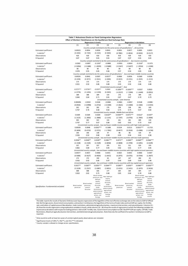
We also conducted a series of robustness checks. First, from the results of Table 4-6 it

became apparent that, owing to differences in data coverage, the country sample changed

whenever a different set of fundamentals was used. Thus, we re-estimated the regressions by

restricting the country sample to be maintained throughout all specifications, the results of which

are shown in the top three panels of Table 7. The effect of remittances on the equilibrium real

exchange rate remains weak within this stable country sample, even turning negative for low-

income countries, while the inclusion of lower middle income countries again tends to increase

the positive effect of remittances on the real exchange rate. However, that the signs of the

coefficient remain unaltered across specifications implies that the changes in sign observed earlier

had more to do with changes in the country sample than with interactions between the different

fundamentals included or excluded.

18 Note that capital account openness is a necessary but not sufficient condition for the equilibrium real exchange rate to be less sensitive to remittance inflows. It is also necessary for capital markets to price remittances into the risk premia being charged as well. Here capital account openness serves as an imperfect proxy for this effect.

38

(1) (2) (3) (4) (5) (6) (7) (8)

Estimated coefficient 0.00323 0.0054 0.0026 0.0041 0.0055 0.0077 0.0005 0.0023

t-statistic2 (0.4483) (0.7400) (0.2420) (0.3880) (0.7881) (1.0814) (0.0432) (0.2117)

Observations 418 418 418 418 418 418 418 418

R-Squared 0.87 0.87 0.81 0.81 0.87 0.87 0.81 0.81

Estimated coefficient -0.0302 -0.0097 -0.1335* -0.0898 -0.0355 -0.0614 -0.1510* -0.1373

t-statistic2

(-0.5856) (-0.1686) (-1.8593) (-0.9680) (-0.5567) (-0.6427) (-1.9016) (-1.4584)

Observations 80 80 80 80 80 80 80 80

R-Squared 0.978 0.95 0.85 0.86 0.97 0.94 0.85 0.86

Estimated coefficient 0.00193 0.0042 0.0207 0.0227* 0.0006 0.0026 0.0180 0.0206

t-statistic2 (0.1938) (0.3972) (1.5641) (1.6986) (0.0623) (0.2451) (1.2845) (1.4410)

Observations 173 173 173 173 173 173 173 173

R-Squared 0.921 0.92 0.86 0.88 0.93 0.92 0.86 0.88

Estimated coefficient -0.0727*** -0.0726*** -0.0237** 0.0062 -0.1036*** -0.1033*** -0.0157 0.0023

t-statistic2 (-4.9795) (-5.1856) (-2.1599) (0.2883) (-6.9137) (-7.2904) (-1.4440) (0.0953)

Observations 188 188 189 133 176 176 189 133

R-Squared 0.846 0.84 0.71 0.81 0.87 0.87 0.70 0.79

Estimated coefficient 0.000496 -0.0010 0.0106 -0.0084 -0.0061 -0.0057 0.0148 -0.0085

t-statistic2

(0.0503) (-0.0998) (1.0714) (-0.3440) (-0.4621) (-0.4483) (1.5364) (-0.3555)

Observations 262 262 282 170 238 238 281 169

R-Squared 0.767 0.76 0.68 0.82 0.75 0.75 0.67 0.82

Estimated coefficient 0.0189 0.0184 0.0184 0.0218** 0.0344*** 0.0371*** 0.0212* 0.0197*

t-statistic2

(1.3125) (1.2850) (1.3868) (2.1141) (2.7297) (3.0793) (1.7893) (1.9006)

Observations 302 302 322 133 261 261 309 130

R-Squared 0.767 0.77 0.67 0.86 0.82 0.81 0.73 0.87

Estimated coefficient 0.00339 0.0048 0.0262*** -0.1698 0.0134 0.0115 0.0352*** -0.1753

t-statistic2

(0.3404) (0.4710) (2.9721) (-1.7941) (0.4677) (0.3550) (3.4386) (-1.6746)

Observations 106 106 138 47 86 86 126 47

R-Squared 0.926 0.92 0.80 0.98 0.95 0.94 0.81 0.98

Estimated coefficient 0.0336** 0.0340** 0.0339** 0.0381*** 0.0271** 0.0305** 0.0369*** 0.0366***

t-statistic2

(2.1538) (2.2104) (2.2109) (2.8058) (2.0848) (2.3700) (2.6391) (2.6109)

Observations 337 337 337 193 311 311 329 193

R-Squared 0.802 0.80 0.77 0.85 0.82 0.81 0.77 0.85

Estimated coefficient 0.00377 0.0037 0.0068 0.0355 0.0025 0.0055 0.0066 0.0307

t-statistic2

(0.5686) (0.5627) (0.9820) (1.6415) (0.2975) (0.6701) (0.9764) (1.3607)

Observations 172 172 190 65 147 147 184 65

R-Squared 0.916 0.92 0.85 0.97 0.90 0.89 0.85 0.98

Estimated coefficient 0.0317** 0.0307** 0.0355*** 0.0344*** 0.0285** 0.0293** 0.0360*** 0.0350***

t-statistic2

(2.3139) (2.2557) (2.6987) (2.8451) (2.4231) (2.5421) (3.1873) (2.9416)

Observations 308 308 326 177 264 264 304 177

R-Squared 0.810 0.81 0.75 0.88 0.85 0.84 0.78 0.88

Specification: Fundamentals excluded:Black market

premium

Black market

premium,

natura l

dis aster

Black market

premium, rea l

GDP per

capi ta ,

natura l

disas ter,

trade

restrictions,

administered

agricul tura l

prices, net

foreign

Rea l GDP per

capi ta,

natural

dis as ter,

trade

res trictions ,

administered

agricul tural

prices , net

foreign

ass ets

Black market

premium

Black market

premium,

natural

disaster

Black market

premium, rea l

GDP per

capi ta ,

natura l

disas ter,

trade

restrictions ,

administered

agricul tura l

prices, net

foreign

Rea l GDP per

capi ta ,

natura l

dis aster,

trade

res trictions,

adminis tered

agricul tura l

prices , net

foreign

ass ets

1 Only countries with at least ten years of uninterrupted yearly observations are included.

2 Significance levels of 10% (*), 5%(**), and 1% (***) indicated.

3 Country sample is allowed to change across specifications.

Table 7. Robustness Checks on Panel Cointegration Regressions


Effect of Workers' Remittances on the Equilibrium Real Exchange Rate

Country sample restricted to be the same across all specifications1

, all countries

Unrestricted country sample , low and lower-middle-income countries with low capital account openness


, low-income countries


, low and lower-middle-income countries

Unrestricted country sample , Latin America

Unrestricted country sample , Middle East and Africa

Unrestricted country sample3

, Asia

Unrestricted country sample , low and lower-middle-income countries with high capital account openness

Unrestricted country sample , low and lower-middle-income countries with high trade openness

Unrestricted country sample , low and lower-middle-income countries with low trade openness

This table reports the results of Dynamic Ordinary Least Squares regressions of the logarithm of the real effective exchange rate on the ratios to GDP of Official

Aid, Net foreign assets, Government consumption, and workers' remittances; the logarithms of the terms of trade index and real GDP per capita; the fertility

rate; and indices of capital account liberalization, trade restrictions, administered agricultural prices, maximum intervention, and natural disaster. Columns (1) -

(4) show the results regressions using explanatory variables in levels, while columns (5) - (8) show the results of regressions in which the following variables are

expressed as deviations with respect to trading partners: Aid to GDP, Fertility rate, Government Consumption to GDP, Real PPP GDP per capita, CAP100, Trade

Restrictions, Maximum agricultural price intervention, and Administered agricultural prices. Note that only the coefficient for workers' remittances to GDP is

reported.

39

Second, we explored whether there are observable cross-region differences in the effect of

workers’ remittances on the equilibrium real exchange rate. The results are shown in the 4th to 6th

panels of Table 7, which reveal that Asia and the Middle East/Africa stand out as two regions

where the effect is distinct from that of the rest of the world. In the former, the coefficient is

consistently negative and often significant, while in the latter, the effect is closest to the

conventional positive effect, and in most cases is statistically significant.

Third, we sought to identify the possible impact of trade or capital account openness on

the relationship between workers’ remittances and the equilibrium real exchange rate. Broadly

speaking, the predictions of the model were confirmed, as shown in the last four panels of Table

7; among low and lower-middle-income countries, those that are relatively closed—either in trade

or in their capital account19—tend to exhibit the more robust conventional result that a permanent

increase in remittance inflows would lead to an appreciation of the equilibrium real exchange rate.

For more open countries, this effect tends to be smaller and much more uncertain.

As a final robustness check, we ran standard panel data regressions,20 including interaction

terms between workers’ remittances and four different factors that might affect their relationship

with the real exchange rate: real GDP per capita, capital account openness, trade openness

(measured as total trade to GDP), and the degree of procyclicality of workers’ remittances. The

19 Countries are identified as having high or low trade or capital account openness based on whether their value for the trade/capital account openness lies above or below the full country sample median. 20 In addition to the fixed effects and OLS regressions reported, we also ran random effects regressions, but Hausman specification tests overwhelmingly favored fixed effects over random effects.

40

latter was calculated as the correlation between HP-filtered series of workers’ remittances and

home country GDP, both measured in U.S. dollars.21 In order to account for possible endogeneity

of workers’ remittances, we estimated a first-stage regression in which average host country per

capita GDP, the ratio of the stock of outward migrants to total population, and the average ratio of

remittances to GDP in all other remittance receiving countries were used as instruments, and then

used the fitted values of remittances in the second stage regressions for the real exchange rate.

The results of the first stage regression, along with FE-IV and OLS-IV regressions, are reported in

Table 8. All specifications in columns (1) – (8) use the full set of fundamentals, as in column (1)

in Tables 4-6. Also as in the previous tables, columns (1) – (4) contain regressions in levels, and

(5) – (8) include regressions in deviations.

In general, the results show that it is difficult to capture the impact of these country

characteristics on the remittance-real exchange rate relationship in a simple linear fashion. The

only significant interaction that arises is with real GDP per capita; the richer the country, the more

likely it will display the expected positive relationship. Although both procyclicality and capital

account openness behave in the expected direction—the greater the countercyclicality of

remittances or the openness of the capital account22, the smaller the effect on the real exchange

rate—the interaction coefficient is not statistically significant.

21 Since this variable yielded a single value per country, it was necessary to estimate the regression via OLS. 22 Similar results were obtained when interacting the trade restrictions variable with workers’ remittances; greater trade openness was associated with a smaller appreciation effect, but this interaction was not statistically significant.

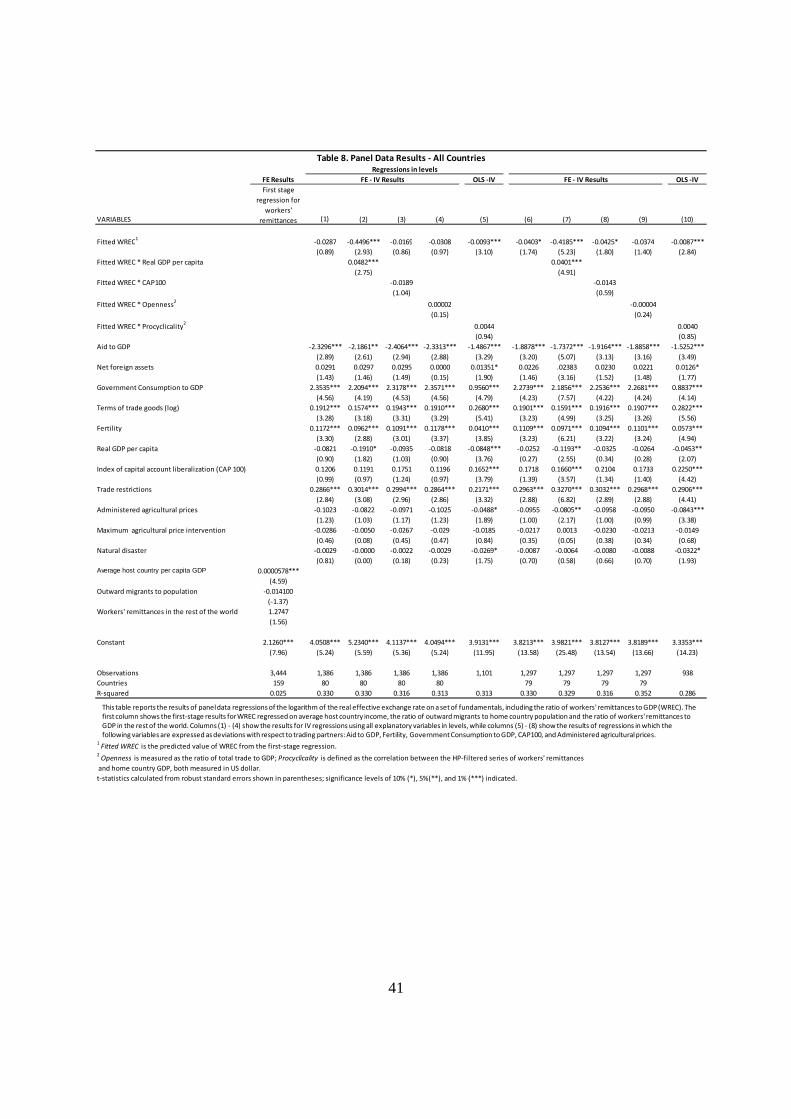
41

FE Results OLS -IV OLS -IV

VARIABLES

First stage

regression for

workers'

remittances (1) (2) (3) (4) (5) (6) (7) (8) (9) (10)

Fitted WREC1

-0.0287 -0.4496*** -0.0169 -0.0308 -0.0093*** -0.0403* -0.4185*** -0.0425* -0.0374 -0.0087***

(0.89) (2.93) (0.86) (0.97) (3.10) (1.74) (5.23) (1.80) (1.40) (2.84)

Fitted WREC * Real GDP per capita 0.0482*** 0.0401***

(2.75) (4.91)

Fitted WREC * CAP100 -0.0189 -0.0143

(1.04) (0.59)

Fitted WREC * Openness2

0.00002 -0.00004

(0.15) (0.24)

Fitted WREC * Procyclicality2

0.0044 0.0040

(0.94) (0.85)

Aid to GDP -2.3296*** -2.1861** -2.4064*** -2.3313*** -1.4867*** -1.8878*** -1.7372*** -1.9164*** -1.8858*** -1.5252***

(2.89) (2.61) (2.94) (2.88) (3.29) (3.20) (5.07) (3.13) (3.16) (3.49)

Net foreign assets 0.0291 0.0297 0.0295 0.0000 0.01351* 0.0226 .02383 0.0230 0.0221 0.0126*

(1.43) (1.46) (1.49) (0.15) (1.90) (1.46) (3.16) (1.52) (1.48) (1.77)

Government Consumption to GDP 2.3535*** 2.2094*** 2.3178*** 2.3571*** 0.9560*** 2.2739*** 2.1856*** 2.2536*** 2.2681*** 0.8837***

(4.56) (4.19) (4.53) (4.56) (4.79) (4.23) (7.57) (4.22) (4.24) (4.14)

Terms of trade goods (log) 0.1912*** 0.1574*** 0.1943*** 0.1910*** 0.2680*** 0.1901*** 0.1591*** 0.1916*** 0.1907*** 0.2822***

(3.28) (3.18) (3.31) (3.29) (5.41) (3.23) (4.99) (3.25) (3.26) (5.56)

Fertility 0.1172*** 0.0962*** 0.1091*** 0.1178*** 0.0410*** 0.1109*** 0.0971*** 0.1094*** 0.1101*** 0.0573***

(3.30) (2.88) (3.01) (3.37) (3.85) (3.23) (6.21) (3.22) (3.24) (4.94)

Real GDP per capita -0.0821 -0.1910* -0.0935 -0.0818 -0.0848*** -0.0252 -0.1193** -0.0325 -0.0264 -0.0453**

(0.90) (1.82) (1.03) (0.90) (3.76) (0.27) (2.55) (0.34) (0.28) (2.07)

Index of capital account liberalization (CAP 100) 0.1206 0.1191 0.1751 0.1196 0.1652*** 0.1718 0.1660*** 0.2104 0.1733 0.2250***

(0.99) (0.97) (1.24) (0.97) (3.79) (1.39) (3.57) (1.34) (1.40) (4.42)

Trade restrictions 0.2866*** 0.3014*** 0.2994*** 0.2864*** 0.2171*** 0.2963*** 0.3270*** 0.3032*** 0.2968*** 0.2906***

(2.84) (3.08) (2.96) (2.86) (3.32) (2.88) (6.82) (2.89) (2.88) (4.41)

Administered agricultural prices -0.1023 -0.0822 -0.0971 -0.1025 -0.0488* -0.0955 -0.0805** -0.0958 -0.0950 -0.0843***

(1.23) (1.03) (1.17) (1.23) (1.89) (1.00) (2.17) (1.00) (0.99) (3.38)

Maximum agricultural price intervention -0.0286 -0.0050 -0.0267 -0.029 -0.0185 -0.0217 0.0013 -0.0230 -0.0213 -0.0149

(0.46) (0.08) (0.45) (0.47) (0.84) (0.35) (0.05) (0.38) (0.34) (0.68)

Natural disaster -0.0029 -0.0000 -0.0022 -0.0029 -0.0269* -0.0087 -0.0064 -0.0080 -0.0088 -0.0322*

(0.81) (0.00) (0.18) (0.23) (1.75) (0.70) (0.58) (0.66) (0.70) (1.93)

Average host country per capita GDP 0.0000578***

(4.59)

Outward migrants to population -0.014100

(-1.37)

Workers' remittances in the rest of the world 1.2747

(1.56)

Constant 2.1260*** 4.0508*** 5.2340*** 4.1137*** 4.0494*** 3.9131*** 3.8213*** 3.9821*** 3.8127*** 3.8189*** 3.3353***

(7.96) (5.24) (5.59) (5.36) (5.24) (11.95) (13.58) (25.48) (13.54) (13.66) (14.23)

Observations 3,444 1,386 1,386 1,386 1,386 1,101 1,297 1,297 1,297 1,297 938

Countries 159 80 80 80 80 79 79 79 79

R-squared 0.025 0.330 0.330 0.316 0.313 0.313 0.330 0.329 0.316 0.352 0.286

1 Fitted WREC is the predicted value of WREC from the first-stage regression.

2 Openness is measured as the ratio of total trade to GDP; Procyclicality is defined as the correlation between the HP-filtered series of workers' remittances

and home country GDP, both measured in US dollar.

t-statistics calculated from robust standard errors shown in parentheses; significance levels of 10% (*), 5%(**), and 1% (***) indicated.

Table 8. Panel Data Results - All Countries

Regressions in levels

FE - IV Results FE - IV Results

This table reports the results of panel data regressions of the logarithm of the real effective exchange rate on a set of fundamentals, including the ratio of workers' remittances to GDP (WREC). The

first column shows the first-stage results for WREC regressed on average host country income, the ratio of outward migrants to home country population and the ratio of workers' remittances to

GDP in the rest of the world. Columns (1) - (4) show the results for IV regressions using all explanatory variables in levels, while columns (5) - (8) show the results of regressions in which the

following variables are expressed as deviations with respect to trading partners: Aid to GDP, Fertility, Government Consumption to GDP, CAP100, and Administered agricultural prices.

42

V. Summary and conclusions

The effects of a permanent increase in inflows of workers’ remittances on a country’s

long-run equilibrium real exchange rate would appear to be rather straightforward: thinking of

such remittances as equivalent to an exogenous inflow of international transfers suggests that an

appreciation in the long-run equilibrium real exchange rate would be required to maintain internal

and external balance: maintaining external balance requires an increase in domestic absorption to

compensate for the higher level of income, and the higher level of domestic absorption in turn

requires a real exchange rate appreciation to clear the nontraded goods market. This analysis

motivates the concern that the increase in remittance receipts that many developing countries have

experienced in recent years would be associated with “Dutch disease” problems.

This paper has argued, however, that the effects of permanent changes in remittance

receipts on the real exchange rate may be more complicated than this analysis would suggest.

First, the impact of remittance flows on the equilibrium real exchange rate will tend to be

small in highly open economies with flexible labor markets in which the traded and nontraded

goods sectors employ similar factors that can be readily reallocated between the two sectors with

minimal frictions. In this case increased absorption will be largely dissipated in demand for

traded goods, and small changes in the real exchange rate will be sufficient to satisfy whatever

additional demand is created for nontraded goods.

43

Second, if remittance receipts are only partly autonomous, so that such receipts are

partially driven by changes in domestic real income in countercyclical fashion, the effects of an

exogenous increase in remittance receipts on the long-run equilibrium real exchange rate will tend

to be muted. The reason is that higher remittance receipts induce an increase in domestic real

output, which in turn tends to discourage such receipts. The effect is to ameliorate, but not

entirely offset, the traditional effect of changes in remittance receipts on the long-run equilibrium

real exchange rate.

Third, if the risk premium that a country faces in international capital markets is

(favorably) affected by remittance receipts – as the evidence suggests it is -- then the reduced cost

of international borrowing in response to larger remittance inflows will induce the country to

reduce its international net investment position in the long run, and the reduced net interest

receipts induced by the deterioration in the net investment position would tend to offset the effects

of the remittance receipts on the equilibrium real exchange rate. This channel could completely

eliminate the effect of changes in the permanent value of workers’ remittances on the long-run

equilibrium real exchange rate.

Finally, if remittance receipts are fully (rather than just partially) devoted to expenditures

on traded goods, changes in such receipts would have no effect on the long-run equilibrium real

exchange rate in a nonmonetary economy, and in a monetary economy the standard presumption

that higher remittance receipts would tend to appreciate the long-run equilibrium real exchange

rate could even be reversed, depending on the form in which transactions costs are incurred.

44

The message from this analysis is not that the standard presumption about the effects of

workers’ remittances on the equilibrium real exchange rate is wrong, but rather that it is too

simple. Workers’ remittances may affect the equilibrium real exchange rate through a variety of

macroeconomic channels, and the particular channels that are operative in any specific country

case will determine the quantitative – and perhaps even the qualitative – effect of changes in

flows of worker remittances on the real exchange rate.

The empirical evidence on this issue, featuring both single-country and panel studies, is

mixed. Accordingly, we have conducted our own panel estimation, employing a larger set of

countries, more recent data, and a more comprehensive set of real exchange rate fundamentals

than have been used in previous studies. Most importantly, our panel cointegration methodology

explicitly focuses on identifying the effects of workers’ remittances on the equilibrium real

exchange rate in the recipient countries. We find that the effect of remittance flows on the

equilibrium real exchange rate is not very robust, with the sign and statistical significance of the

effect depending on the country sample being analyzed and, to a lesser extent, on the specific set

of non-remittance fundamentals included in the cointegrating equation. Our robustness checks

provide support for the model’s predictions that countries with low trade and/or capital account

openness would be most likely to exhibit the conventional appreciation effect of remittances,

although we recognize that it is difficult to capture these interactions with a simple linear

relationship. We also detect regional differences, with the Middle East/North African countries

most likely to experience the conventional upward effect of rising remittance inflows on the real

exchange rate, and Asian countries less likely to do so. Finally, in general, richer remittance

45

receiving countries—perhaps because the lower trade openness dominates their greater integration

into international capital markets23—are more likely to exhibit the conventional effect.

Most importantly, even when the estimated effect of remittance flows on the equilibrium

real exchange rate exhibits the conventional sign and is precisely estimated, the magnitude of this

effect is consistently very small. This suggests that Dutch disease problems, in the form of a

contraction of traded goods production and a reduced flow of whatever positive production

externalities may be generated by such production, may not be a necessary side effect of

remittance inflows. In that case, the beneficial short-run effects of remittance inflows on

economic welfare in the recipient countries through higher and more stable levels of consumption

may not come at the expense of reduced long-run growth.

23 Recall that what matters is the pricing of risk; a country can have a very open capital account, but if markets are not pricing its permanent remittance inflows into the risk premium, then there will be no impact on the remittance-equilibrium real exchange rate relationship.

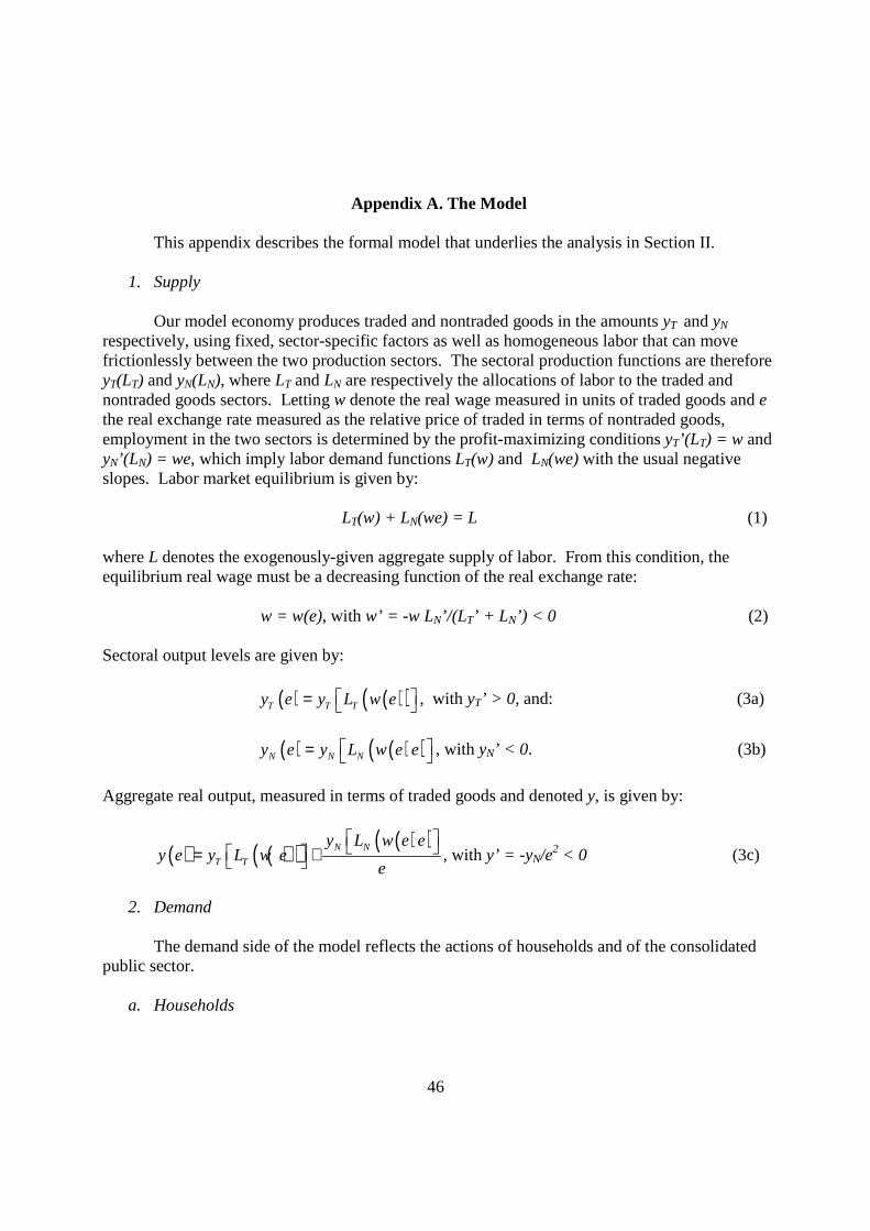
46

Appendix A. The Model

This appendix describes the formal model that underlies the analysis in Section II.

1. Supply Our model economy produces traded and nontraded goods in the amounts yT and yN

respectively, using fixed, sector-specific factors as well as homogeneous labor that can move frictionlessly between the two production sectors. The sectoral production functions are therefore yT(LT) and yN(LN), where LT and LN are respectively the allocations of labor to the traded and nontraded goods sectors. Letting w denote the real wage measured in units of traded goods and e the real exchange rate measured as the relative price of traded in terms of nontraded goods, employment in the two sectors is determined by the profit-maximizing conditions yT’(LT) = w and yN’(LN) = we, which imply labor demand functions LT(w) and LN(we) with the usual negative slopes. Labor market equilibrium is given by:

LT(w) + LN(we) = L (1) where L denotes the exogenously-given aggregate supply of labor. From this condition, the equilibrium real wage must be a decreasing function of the real exchange rate: w = w(e), with w’ = -w LN’/(LT’ + L N’) < 0 (2) Sectoral output levels are given by: ( ) ( )( )T T Ty e y L w e = , with yT’ > 0 , and: (3a)

( ) ( )( )N N Ny e y L w e e = , with yN’ < 0 . (3b)

Aggregate real output, measured in terms of traded goods and denoted y, is given by:

( ) ( )( ) ( )( )N N

T T

y L w e ey e y L w e

e

= + , with y’ = -yN/e2 < 0 (3c)

2. Demand

The demand side of the model reflects the actions of households and of the consolidated public sector.

a. Households

47

Households receive income from domestic production and remittances, out of which they pay lump-sum taxes, consume, and save. Their saving can be allocated to the accumulation of net foreign bonds and/or domestic money, and portfolio equilibrium is assumed to hold continuously.

The problem faced by the representative household can be described as follows: At each

instant, it allocates its net worth, denoted a, between net foreign bonds fH and domestic money m, subject to the balance sheet constraint: a = fH + m. (4) Foreign bonds pay the (nominal and real) interest rate r* , and the holding of money is motivated by a desire to avoid the transaction costs associated with consumption. Such costs are given by:

( ) ( ), mT m c ccτ= , with τ’ < 0 and τ’’ > 0 (5)

where c is total consumption expenditure measured in terms of traded goods. This specification postulates that transactions costs are homogeneous in the real money stock and consumption spending, that transaction costs per unit of consumption are a decreasing function of the stock of money per unit of consumption, but that the productivity of money in reducing transactions costs is subject to diminishing returns. The accumulation of household wealth over time is the sum of household saving and net real capital gains or losses. It can be expressed in the form of the budget constraint:

( )* 1Ha y rem r f t cτ= + + − − +& (6)

where rem denotes the flow of remittance receipts and t denotes real (lump-sum) taxes paid by households. The path of consumption expenditure is determined by the maximization over an infinite horizon of an additively-separable utility function in which future felicity is discounted at the constant rate of time preference ρ. Total consumption expenditure consists of spending on traded goods, denoted cT, and on nontraded goods cN, which are the direct sources of utility for the household. Thus total consumption expenditure c is given by c = cT + cN/e. The felicity function is of the constant-relative-risk-aversion type, and is assumed to be Cobb-Douglas in consumption of traded and nontraded goods. It therefore takes the form:

( ) ( ) ( )11

, ,1T N

e cU c c v e c

σθ

σ

−−Κ= =

− (7)

where θ and σ are positive parameters, the former representing the share of traded goods consumption in total consumption expenditure, and the latter the inverse of the intertemporal rate of substitution. The Cobb-Douglas specification implies that consumption expenditure is allocated in constant shares between the two types of consumption goods:

48

cT = θc cN = (1 – θ)ec (8) Using these in (7) we can express the indirect utility function in the form:

( ) ( ) ( )11

, ,1T N

e cU c c v e c

σθ

σ

−−Κ= =

− (9)

where κ is a positive constant. The household’s problem can therefore be stated as follows: it chooses paths for consumption expenditure c and money m so as to maximize:

( ) ( ) ( ) ( )11

0

, , exp1T N

e cU c c v e c t dt

σθ

ρσ

−−∞ Κ= =

−∫ (10)

subject to the flow budget constraint (6) and a transversality condition. These can conveniently be written as:

( ) ( )( )* 1 ma y rem r a m t ccτ= + + − − − +& (6’)

*

0

lim exp 0a r dt∞

− = ∫ (11)

where r* is the real interest rate on foreign bonds, measured in terms of traded goods. The present-value Hamiltonian for this problem is:

( ) ( )

11

exp1

e cH a t

σθ

λ ρσ

−− = Κ + − −

&

with first-order conditions:

( ) ( )( )'1 0m me c cc cγ σ λ τ τ−Κ − + − = (12a)

( ) *m icτ− = (12b)

( )*rλ ρ λ− = & (12c)

49

The dynamics of household consumption expenditure are determined by these conditions,

as well as the budget constraint (6’) and transversality condition (11). Equation (12b) implies the money demand function:

m = h(r*)c, h’ < 0 (13)

By differentiating equation (12a) with respect to time, and using (12b), (12c), and (13 ), we can derive the household’s Euler equation in the form:

( )( )

( )( ) ( )

1 * * *

* * *1

er h r r cec

h r r h r

γσ ρ

τ

− − − +=

+ −

&&

& (14)

The consolidated public sector includes both the government and the central bank. The

sole function of the central bank is to maintain the exchange rate parity. It does so by exchanging domestic and foreign currency for each other on demand in unlimited amounts at the fixed parity. Its balance sheet is thus given by fC = m, where fC is the real stock of foreign exchange reserves -- i.e., the stock of foreign bonds held by the central bank measured in units of tradable goods. Interest receipts on these bonds are transferred to the government. The latter, in addition to the central bank’s interest receipts, receives the lump-sum taxes that are collected from households. Like the households, the government has to respect an intertemporal budget constraint. For concreteness, we’ll assume that it does so in a particularly simple way -- by maintaining a continuously balanced budget. Thus the consolidated budget constraint of the government and the central bank can be expressed as: t = i*fC = i*m (15) The model is closed with two equilibrium conditions. The first is an arbitrage relationship describing the terms on which the rest of the world will lend to the domestic economy, and the second characterizes equilibrium in the market for nontraded goods. Though the home country is a price taker in the world goods market, its financial liabilities are not perfect substitutes for those of the rest of the world. The interest rate at which residents of the country can borrow abroad thus reflects a risk premium which is an increasing function of the share of the country’s liabilities held in world financial portfolios. This is incorporated in the model in the form of an upward-sloping supply-of-funds schedule relating the external interest rate confronted by the country’s residents, r* , to the country’s net international indebtedness, as well as to world financial conditions, measured by the exogenous world interest rate rW. The specific formulation expresses r* as the sum of the world interest rate and a risk premium p that is inversely related to the country’s aggregate net international investment position. Since both the government and the central bank maintain continuously balanced budgets the latter must be equal to the net worth of the household sector. We can therefore write

50

the supply of funds schedule as: r* = rW + p(a) (16) Finally, with no exhaustive public spending, the equilibrium condition in the market for nontraded goods can simply be expressed as: yN(e) = cN = (1 – θ)ec (17) For future reference, it is worth noting that the specification of equilibrium in the nontraded goods market (17) implies that all production of nontraded goods is available for consumption. We are implicitly assuming, therefore, that the transaction costs associated with consumption are incurred in the form of traded goods.24 Equation (17) can be solved for the value of the real exchange rate that clears the nontraded goods market, conditional on the value of private spending c. This short-run equilibrium real exchange rate is given by: e = e(c) (18)

( )

( )'

'

10

1N

ee

y c

θθ

−= <

− −

The real exchange rate that solves equation (18) is a short-run equilibrium one in the sense that it clears the market for nontraded goods for a given value of private consumption expenditure c. Thus, this real exchange rate will be sustainable only to the extent that c is itself sustainable. To assess the sustainable value of c requires solving the model for the path of c over time. Before describing the determinants of the steady-state equilibrium real exchange rate in this model, we need to establish that the model possesses a stable steady-state equilibrium. For the purpose of solving the model, the two key dynamic equations are the household budget constraint (6) and its Euler equation (14). Consider the former. By using the definition of real output from equation (3), the money demand function (13), the government budget constraint (15), the supply of funds schedule (14), and the expression for the short-run equilibrium real exchange rate (17), equation (6) can be manipulated into the form:

( ) ( ) ( )( )( )( )T w wa y e rem r p a h r p a cτ θ = + + + − + + & (19)

Using the nontraded goods market equilibrium condition (18) to eliminate e, this becomes:

24 This assumption is made for concreteness and simplicity. It does not affect the results derived below.

51

( ) ( ) ( )( )( )( )T w wa y e c rem r p a h r p a cτ θ = + + + − + + & (20)

The properties of this equation can be summarized as follows:

( ), ,a a c a rem=& (21)

( )'1 1 0Ta y e τ θ= − − <

* ' ' ' '2 0a r p a h p cτ= + − >

a3 = 1

Before proceeding similarly with equation (14), note first that ( )* 'r p a a=& & , and

1e e c=& & . Substituting these and equation (21) into (14) we have:

( ) ( ) ( ) ( )( )( )( )( )( ) ( )( ) ( )( )

* '

1, ,

1

w

w w w

er p a h r p a p a a c a rem cech r p a r p a h r p a

ρ γσ

τ−

+ − − + +=

+ + − + +

&

& (22)

which can be solved for c& to yield: ( ), ,c c c a rem=& (23)

'

11 0

a hpc = <

Σ

( )'

22

1p hac

− −=

Σ

'

3 0hp

c = <Σ

where ( )* 11 0e

r he c

υ Φ Σ = + − − <

.

Equations (21) and (23) represent a system of two differential equations in the variables c and a. The former is a “jump” variable, while the latter is predetermined. The steady-state equilibrium of this system is the combination (c*, a*) which satisfies 0c a= =& & . Stability is determined by the sign of the determinant of the transition matrix of the system (21) and (22) linearized around the steady-state equilibrium values (c*, a*). It is straightforward to show that this determinant is negative, so its roots must be of opposite sign, implying that the equilibrium (c*, a*) is saddlepoint stable. Having established that our model possesses a stable steady-state equilibrium, we can now

52

examine the properties of that equilibrium. To do so, begin by noting from equation (22) that the imposition of the long-run equilibrium conditions c a=& & in that equation implies: rW + p(a) = ρ (24) Since rW and r are both exogenous, this equation determines the equilibrium value of the country’s net international investment position, a*. Because the premium p is a decreasing function of the net international investment position, this equation states that countries with a high rate of time preference will be driven to have a smaller stock of net external claims in long-run equilibrium than those with lower rates of time preference. Since r* = r W + p(a*), this equation in turn implies that the equilibrium value of the domestic real interest rate will be given by: r* = ρ (25) This value of r* pins down the long-run values of consumption velocity h and transactions cost per unit of consumption J: h* = h(r*) = h( ρ) (26) τ* = τ[h(r*)] = τ[h(ρ)] (27)

With these results in hand, we can now describe the conditions that characterize the equilibrium real exchange rate in this model. Using (25)-(27) in equation (19) yields: 0 = yT(e) + rem +r*a* - (τ* + θ)c (28) This is the external balance condition in our model. Recalling that cT = θc, and that transactions costs are assumed to be incurred in traded goods, aggregate demand for traded goods is given by θc, and aggregate supply is (yT - Jc). Thus aggregate excess supply of traded goods, equal to the real trade balance surplus, is (yT - Jc) - θc = yT - (J +θ)c. Adding the receipt of remittances and interest payments from abroad (recall that a* is the country’s net international investment position) yields the current account, measured in units of traded goods, which is the right-hand side of (28). Condition (28) therefore states that in zero-growth noninflationary steady-state equilibrium, the current account must be in balance. Since yT is increasing in the real exchange rate e, and since an increase in consumption expenditure reduces the trade surplus, the set of combinations of e and c that satisfies (28) is plotted as the positively-sloped external balance locus EB in Figure 4.

From (18) and (28), the effect of a change in exogenous remittance inflows on the equilibrium real exchange rate is given by:

53

( )

*'

'

10

1T

NN

e

remy

ye y e

τ θ

θ

∂ = − <+∂ −

− −

(29)

The discussion in Section II.1 of the determinants of the quantitative effects of remittances on the equilibrium real exchange rate follow from this equation. The extensions of the model follow:

1. Induced remittances A simple linear function describing remittances as induced by domestic real income is: rem = µ0 + µ1y. (30) Under this assumption equation (19) becomes:

( ) ( )( ) ( )( )( )0 1T w wa y e y r p a h r p a cµ µ τ θ = + + + + − + + & (31)

and from equation (3c), which establishes that y’ < 0, it follows that the real exchange rate has a stronger impact on the external balance condition in this case.

2. Effects operating through the risk premium Rewrite the international interest rate faced by the domestic economy as: r* = r W + p(a + rem/r*) (32) Note that equation (26) must continue to hold in long-run equilibrium. Substituting (26) into (32) and differentiating with respect to rem yields:

( )

0

rema

rem

ρ∂ +=

∂, so ( ) *

1 1a

rem rρ∂ = − = −

∂ (33)

The external balance condition can now be written as: 0 = yT(e) + rem + r*a*(rem) – (τ* + θ)c (34) which differs from (28) only in that the country’s long-run net investment position a* is a

function of the level of remittances, with *

*

1a

rem r

∂ = −∂

, as given by (33). Differentiating (34) with

54

respect to rem yields the result that changes in rem have no effect on the external balance condition.

3. Direct effects on household utility functions

We can capture the spending of remittances on tradables in the model by writing the representative household’s utility function as: U(cT, cN) =v(e, c)= [cT – rem)θ cN

1 – θ] 1 – σ (7’) 1 - σ which implies that consumption of traded and nontraded goods respectively are given by: cT = θ(c – rem) + rem (8’) cN = (1 – θ)e(c – rem) The equilibrium condition in the market for nontraded goods thus becomes: yN(e) = cN = (1 – θ)e(c – rem) (17’) and the external balance condition (28) can be written as: 0 = yT(e) + rem +r*a* - τ*c – [θ(c – rem) + rem] which is equivalent to: 0 = yT(e) + rem +r*a* - τ*c – θ(c – rem) (28’) The analysis in the text follows directly from equations (17’) and (28’).

55

Appendix B. Country Sample The countries are classified as high, upper middle income, lower middle income, and low income countries based on the World Bank classification. The high- and upper-middle-income countries in the sample are New Zealand, Greece, Australia, Norway, Switzerland, United Kingdom, Canada, Germany, Spain, Sweden, Portugal, France, Austria, Denmark, Czech Republic, Belgium, Ireland, Finland, United States, Korea, Japan, Netherlands, Italy, Luxembourg, Saudi Arabia, Singapore, Trinidad and Tobago, United Arab Emirates, Israel, Slovenia, Estonia, Romania, Mexico, Russia, Oman, Slovak Republic, Costa Rica, Uruguay, Brazil, Lithuania, Bulgaria, South Africa, Mauritius, Latvia, Croatia, Malaysia, Libya, Panama, Hungary, Venezuela, Rep. Bol., Gabon, Kazakhstan, Botswana, Turkey, Poland, and Lebanon. The low income countries in the sample are Bangladesh, Lao People's Democratic Republic, Eritrea, Tajikistan, Mongolia, Tanzania, India, Vietnam, Uganda, Kyrgyz Republic, Sierra Leone, Democratic Republic of Congo, Mozambique, Central African Republic, Guinea, Zambia, Zimbabwe, Niger, Ethiopia, Kenya, Burkina Faso, Benin, Ghana, Nigeria, Mali, Madagascar, Sudan, Côte d'Ivoire, Cambodia, Haiti, Togo, Pakistan, Rwanda, Nepal, Burundi, Islamic Republic of Afghanistan, Malawi, Republic of Yemen, Chad, The Gambia, Mauritania, Senegal, Uzbekistan, and Papua New Guinea. The lower middle income countries in the sample are Macedonia FYR, Islamic Republic of Iran, Republic of Congo, Bosnia & Herzegovina, El Salvador, Nicaragua, Lesotho, Thailand, Georgia, Cameroon, Angola, Albania, Dominican Republic, Algeria, Belarus, Ukraine, Armenia, Philippines, Moldova, Turkmenistan, Paraguay, Namibia, Tunisia, Morocco, Syrian Arab Republic, Peru, Swaziland, Guatemala, Honduras, Sri Lanka, Indonesia, Egypt, Jamaica, Bolivia, Ecuador, People’s Republic of China, Colombia, and Jordan.

56

References Acosta, Pablo, Emmanuel Lartey, and Federico Mandelman (2007), “Remittances and the Dutch Disease,” Federal Reserve Bank of Atlanta Working paper 2007-8 (April). Acosta, Pablo, Nicole Rae Baerg, and Federico Mandelman (2009), “Financial Development, Remittances, and Real Exchange Rate Appreciation,” Federal Reserve Bank of Atlanta Economic Review, Number 1, pp. 1-12. Amuedo-Dorantes, Catalina, and Susan Pozo (2004), “Workers’ Remittances and the Real Exchange Rate: A Paradox of Gifts,” World Development 32 (8), pp. 1407-17. Bourdet, Yves, and Hans Falck (2003), “Emigrant’s Remittances and Dutch Disease in Cape Verde,” Working Paper Series 11 (Kristianstad, Sweden: Kristianstad University College). Chami, Ralph, Adolfo Barajas, Tomas Cosimano, Connel Fullenkamp, Michael Gapen, and Peter Montiel (2008), Macroeconomic Consequences of Remittances (with, IMF Occasional Paper Number 259 (2008). Christiansen, Lone, Alessandro Prati, Luca Antonio Ricci, and Thierry Tressel (2009), “External Balance in Low-Income Couintries,” International Monetary Fund Working Paper WP/09/221 October). Faini, Riccardo (1994), “Workers’ Remittances and the Real Exchange Rate: A Quantitative Framework,” Journal of Population Economics 7(2), pp. 235-245. Hinkle, Lawrence and Peter Montiel (1999), Exchange Rate Misalignment: Concepts and Measurement for Developing Countries (Oxford: Oxford University Press). Holzner, Mario (2006), “Real Exchange Rate Distortion in Southeast Europe,” Vienna Institute for International Economics, mimeo. Hyder, Zulfiqar and Adil Mahboob (2005), “Equilibrium Real Effective Exchange Rate and Real Exchange Rate Misalignment in Pakistan,” State Bank of Pakistan, mimeo. International Monetary Fund (2005), World Economic Outlook (April), Chapter II. Izquierdo, Alejandro and Peter J. Montiel (2006), “Remittances and Equilibrium Real Exchange Rates in Six Central American Countries,” Williams College, mimeo.

57

Lartey, Emmanuel, Federico Mandelman, and Pablo Acosta (2008), “Remittances, Exchange Rate Regimes, and the Dutch Disease: A Panel Data Analysis,” Federal Reserve Bank of Atlanta Working paper 2008-12 (March) Lopez, Humberto, Luis Molina and Maurizio Bussolo (2007), “Remittances and the Real Exchange Rate,” World Bank Policy Research Working Paper 4213 (April). Montiel, Peter J. (1999), “Determinants of the Long-Run Equilibrium Real Exchange Rate: An Analytical Model,” in L. Hinkle and P. Montiel, eds., Exchange Rate Misalignment: Concepts and Measurement for Developing Countries (Oxford: Oxford University Press) Pesaran, Hashem (2007), “A Simple Panel Unit Root Test in the Presence of Cross-Sectional Dependence,” Journal of Applied Econometrics, Vol. 22, pp. 265-312. Rajan, Raghuram and Arvind Subramanian (2005), “What Undermines Aid’s Impact on Growth?” IMF Working Paper WP/05/126 (June), NBER Working Paper 11657 (October).. Saadi-Sedik, Tahsin, and Martin Petri (2006), “To Smooth or Not to Smooth: The Impact of Grants and Remittances on the Equilibrium Real Exchange Rate in Jordan,” IMF Working paper WP/06/257. Winters, L.A. and Pedro M.G. Martens (2004), “When Comparative Advantage Is Not Enough: Business Costs In Small Remote Economies,” World Trade Review 3(3), pp. 1-37.

draft september 8, 2010web.williams.edu/economics/wp/montielremittancesandtherealexcha… · the...

Documents