risk, return, and equilibrium: empirical tests eugene f...

Risk, Return, and Equilibrium: Empirical Tests

Eugene F. Fama; James D. MacBeth

The Journal of Political Economy, Vol. 81, No. 3. (May - Jun., 1973), pp. 607-636.

Stable URL:

http://links.jstor.org/sici?sici=0022-3808%28197305%2F06%2981%3A3%3C607%3ARRAEET%3E2.0.CO%3B2-J

The Journal of Political Economy is currently published by The University of Chicago Press.

Your use of the JSTOR archive indicates your acceptance of JSTOR's Terms and Conditions of Use, available athttp://www.jstor.org/about/terms.html. JSTOR's Terms and Conditions of Use provides, in part, that unless you have obtainedprior permission, you may not download an entire issue of a journal or multiple copies of articles, and you may use content inthe JSTOR archive only for your personal, non-commercial use.

Please contact the publisher regarding any further use of this work. Publisher contact information may be obtained athttp://www.jstor.org/journals/ucpress.html.

Each copy of any part of a JSTOR transmission must contain the same copyright notice that appears on the screen or printedpage of such transmission.

The JSTOR Archive is a trusted digital repository providing for long-term preservation and access to leading academicjournals and scholarly literature from around the world. The Archive is supported by libraries, scholarly societies, publishers,and foundations. It is an initiative of JSTOR, a not-for-profit organization with a mission to help the scholarly community takeadvantage of advances in technology. For more information regarding JSTOR, please contact [email protected].

http://www.jstor.orgSun Oct 21 07:55:40 2007

http://links.jstor.org/sici?sici=0022-3808%28197305%2F06%2981%3A3%3C607%3ARRAEET%3E2.0.CO%3B2-J

http://www.jstor.org/about/terms.html

http://www.jstor.org/journals/ucpress.html

Risk, Return, and Equilibrium: Empirical Tests

Eugene F. Fama a n d James D. MacBe th University of Chicago

This paper tests the relationship between average return and risk for New York Stock Exchange common stocks. The theoretical basis of the tests is the "two-parameter" portfolio model and models of market equilibrium derived from the two-parameter portfolio model. W e can-no! reject the hypothesis of these models that the pricing of common stocks reflects the attempts of risk-averse investors to hold portfolios that are "efficient" in terms of expected value and dispersion of return. Moreover, the observed "fair game" properties of the coefficients and residuals of the risk-return regressions are consistent with an "efficient capital market1'-that is, a market where prices of securities fully reflect available information.

I. Theoretical Backgrouncl

In the two-parameter portfolio model o f Tobin (1958) , llarkowitz (1959) , and Fama (19655), the capital market is assumed to be perfect in the sense that investors are price takers and there are neither transactions costs nor information costs. Distribution, o f one-period percentage returns on all assets and portfolios are assumed to be normal or to conform to some other two-parameter member of the symmetric stable class. Investors are assumed to be risk averse and to behave as i f they choose among portfolios on the basis o f maximum expected utility. A perfect capital market, investor risk aversion, and tno-parameter return distributions imply the important "efficient set theorem": The optimal portfolio for any investor must be efficient in the sense that no other portfolio with the same or higher expected return has lower dispersion of return.l

Received .Iugust 21, 1971. Final version received ior publication September 2 . 1972. Rcscarch supported by a grant from the Kcltional Science Foundation. The com-

ments of Professors F. Black, L. Fisher, N. Gonedes, M. Jensen, M. Miller, R . Oficer, H. Robcrts, R . Roll, and M. Scholes arc gratciully acknonzledgcd. .I special note of thanks is due to Black. Jensen, and Oflicer.

.ilthough the choicc of dispcrsion parameter is arbitrary, the standard dcviation

608 JOURNAL OF POLITICAL ECONOMY

In the portfolio model the investor looks a t individual assets only in terms of their contributions to the expected value and dispersion, or risk, of his portfolio return. With normal return distributions the risk of portfolio p is measured by the standard deviation, o ( g , ) , of its return, Epl2 and the risk of an asset for an investor who holds p is the contribution of the asset to o(E, ) . If x,, is the proportion of portfolio funds invested in

N N

asset i, o,, = cov(R,, R,) is the covariance between the returns on assets i and j, and N is the number of assets, then

Thus, the contribution of asset i to ~ ( 6 ) - t h a t is, the risk of asset i in the portfolio p-is proportional to

Note that since the weights xi, vary from portfolio to portfolio, the risk of an asset is different for different portfolios.

For an individual investor the relationship between the risk of an asset and its expected return is implied by the fact that the investor's optimal portfolio is efficient. Thus, if he chooses the portfolio m, the fact that m

is efficient means that the weights xi,, i = 1, 2 , . . . ,N, maximize expected portfolio return

subject to the constraints

is common when return distributions are assumed to be normal, whereas an inter-fractile range is usually suggested when returns are generated from some other symmetric stable distribution.

I t is well known that the mean-standard deviation version of the two-parameter portfolio model can be derived from the assumption that investors have quadratic utility functions. But the problems with this approach are also well known. In any case, the empirical evidence of Fama (1965a) , Blume (1970) , Roll (1970) , K. Miller (1971) , and Officer (1971) provides support for the "distribution" approach to the model. For a discussion of the issues and a detailed treatment of the two-parameter model, see Fama and &filler (1972, chaps. 6-8).

We also concentrate on the special case of the two-parameter model obtained with the assumption of normally distributed returns. As shown in Fama (1971) or Fama and Miller (1972, chap. 7 ) , the important testable implications of the general symmetric stable model are the same as those of the normal model.

?Tildes (-) are used to denote random variables. And the one-period percentage return is most often referred to just as the return.

RISK, RETURN, AND EQUILIBRIUM

-P.,

o(R,) = o(R,,) and xi, = 1.

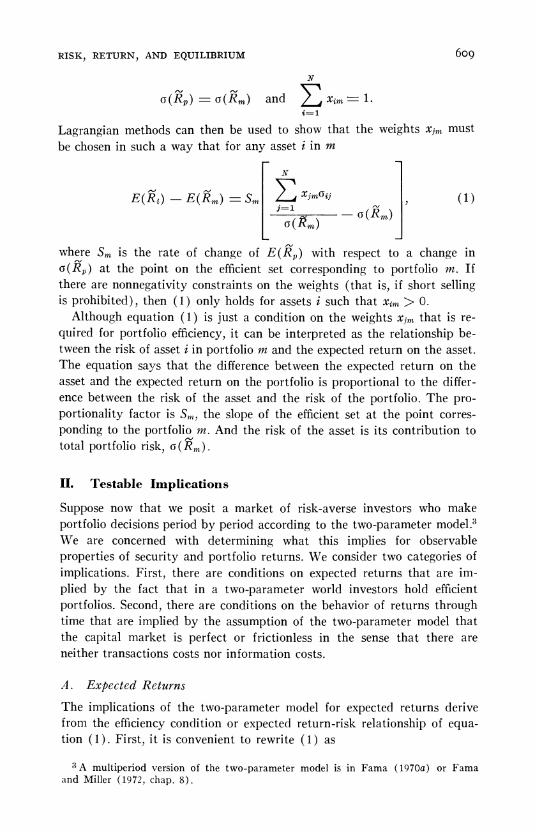
Lagrangian methods can then be used to shon- that the weights x,,,, must be chosen in such a way that for any asset i in m

where S,,, is the rate of change of E ( & ) with respect to a change in o ( g , ) a t the point on the efficient set corresponding to portfolio m. If there are nonnegativity constraints on the weights ( that is, if short selling is prohibited), then (1 ) only holds for assets i such that x,,,, > 0.

Although equation ( 1 ) is just a condition on the weights x,,, that is required for portfolio efficiency, it can be interpreted as the relationship between the risk of asset i in portfolio m and the expected return on the asset. The equation says that the difference between the expected return on the asset and the expected return on the portfolio is proportional to the difference between the risk of the asset and the risk of the portfolio. The pro- portionality factor is S,,,, the slope of the efficient set a t the point corres-ponding to the portfolio nz. And the risk of the asset is its contribution to total portfolio risk, o (g,,,).

11. Testable Implications

Suppose now that we posit a market of risk-averse investors who make portfolio decisions period by period according to the two-parameter model." iVe are concerned with determining what this implies for observable properties of security and portfolio returns. We consider two categories of implications. First, there are conditions on expected returns that are implied by the fact that in a two-parameter world investors hold efficient portfolios. Second, there are conditions on the behavior of returns through time that are implied by the assumption of the two-parameter model that the capital market is perfect or frictionless in the sense that there are neither transactions costs nor information costs.

A . Expected Returns

The implications of the two-parameter model for expected returns derive from the efficiency condition or expected return-risk relationship of equation ( l ) . First, it is convenient to rewrite ( l ) as

"multiperiod version of the two-parameter model is in Fama ( 1 9 7 0 ~ ) or Fama and Miller (1972, chap 8 ) .

- -


where 3-

P i - -

C...01,

- N . ( 3 ) cov(K,Ell!) j= 1 cov ( K t ,En,) /o ( ~ , , , )

-

0 2 ( g i t i ) o"R,, o(R1,,)

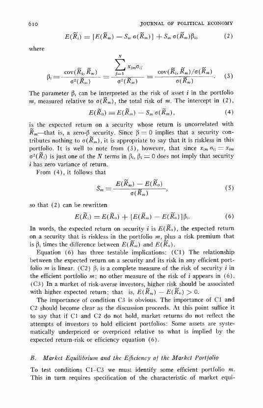
The parameter P, can be interpreted as the risk of asset i in the portfolio nz, measured relative to o ( g i , , ) , the total risk of m. The intercept in ( 2 ) ,

is the expected return on a security whose return is uncorrelated with," Rn,-that is, a zero-p security. Since fi = 0 implies that a security con-tributes nothing to o(R,, , ) , i t is appropriate to say that i t is riskless in this portfolio. I t is well to note from ( 3 ) , however, that since x,,,n, , = x,,,

,-"02(Ri) is just one of the N terms in p,, P, = 0 does not imply that security i has zero variance of return.

From ( 4 ) , i t follows that

so that ( 2 ) can be rewritten

In words, the expected return on security i is E ( R , , ) , the expected return on a security that is riskless in the portfolio nz, plus a risk premium that is p, times the difference between ~ ( g , , , ) and ~ ( g , , ) .

Equation ( 6 ) has three testable implications: ( C l ) The relationship between the expected return on a security and its risk in any efficient portfolio nz is linear. (C2) P, is a complete measure of the risk of security i in the efficient portfolio In; no other measure of the risk of i appears in ( 6 ) . (C3) I n a market of risk-averse investors, higher risk should be associated with higher expected return: that is, ~ ( g , , , ) -E ( R , , ) > 0.

The importance of condition C3 is obvious. The importance of C1 and C2 should become clear as the discussion proceeds. At this point suffice i t to say that if C1 and C2 do not hold, market returns do not reflect the attempts of investors to hold efficient portfolios: Some assets are syste-matically underpriced or overpriced relative to what is implied by the expected return-risk or efficiency equation ( 6 ) .

B. &favket Equilibriu~~z and the E!ficie~cy of the Market Portfolio

T o test conditions CI-C3 we must identify some efficient portfolio In.

This in turn requires specification of the characteristic of market equi-

RISK, RETURN, AND EQUILIBRIUM 611

librium when investors make portfolio decisions according to the two-parameter model.

Assume again that the capital market is perfect. I n addition, suppose that from the information available without cost all investors derive the same and correct assessment of the distribution of the future value of any asset or portfolio-an assumption usually called "homogeneous expectations." Finally, assume that short selling of all assets is allowed. Then Black (1972) has shown that in a market equilibrium, the so-called market portfolio, defined by the weights

total market value of all units of asset i Xl,?l = '

total market value of all assets

is always efficient. Since it contains all assets in positive amounts, the market portfolio is

a convenient reference point for testing the expected return-risk conditions CI-C3 of the two-parameter model. And the homogeneous-expectations assumption implies a correspondence between ex ante assessments of return distributions and distributions of ex post returns that is also re-quired for meaningful tests of these three hypotheses.

C. A Stochastic Model for Returns

Equation ( 6 ) is in terms of expected returns. But its implications must be tested with data on period-by-period security and portfolio returns. We wish to choose a model of period-by-period returns that allows us to use observed average returns to test the expected-return conditions C1-C3, but one that is nevertheless as general as possible. We suggest the following stochastic generalization of ( 6 ):

The subscript t refers to period t, so that ELtis the one-period percentage return on security i from t - 1 to t. Equation ( 7 ) allows 5,t and ylt

to vary stochastically from period to period. The hypothesis of condition C3 is that the expected value of the risk premium TI,, which is the slope

c.,[ ~ ( k , , , t )- E ( K , , t ) ] in ( 6 ) , is positive-that is, E(Tjlt) = E(RrTLt)-~ ( i , ! t )> 0.

The variable p,' is included in ( 7 ) to test linearity. The hypothesis of condition C1 is E(y, , ) = 0,although 72tis also allowed to vary stochastically from period to period. Similar statements apply to the term involving s, in ( 7 ) ,which is meant to be some measure of the risk of security i that is not deterministically related to P,. The hypothesis of condition C2 is E(C;+t)= 0, but can vary stochastically through time.

The disturbance q,, is assumed to have zero mean and to be independenr of all other variables in ( 7 ) .If all portfolio return distributions are to be


normal (or symmetric stable), then the variables Tit, Gt,vlt,S;2t and 73t

must have a multivariate normal (or symmetric stable) distribution.

D. Capital Market Eficiency: The Behavior of Returns through Timc

C1-C3 are conditions on expected returns and risk that are implied by the two-parameter model. But the model, and especially the underlying assumption of a perfect market, implies a capital market that is efficient in the sense that prices at every point in time fully reflect available information. This use of the word efficient is, of course, not to be confused with portfolio efficiency. The terminology, if a bit unfortunate, is a t least standard.

Market efficiency in combination with condition C1 requires that scrutiny of the time series of the stochastic nonlinearity coefficient vlt does not lead to nonzero estimates of expected future values of y2,.Formally, y2t

must be a fair game. In practical terms, although nonlinearities are ob-served ex post, because vIt is a fair game, it is always appropriate for the investor to act ex ante under the presumption that the two-parameter model, as summarized by ( 6 ) , is valid. That is, in his portfolio decisions he always assumes that there is a linear relationship between the risk of a security and its expected return. Likewise, market efficiency in the two- parameter model requires that the non-/3 risk coefficient y i t and the time series of return disturbances q,, are fair games. And the fair-game hypothesis also applies to the time series of - - the[ ~ ( g , , , ) ~ ( g , , ~ ) ] , difference between the risk premium for period t and its expected value.

I n the terminology of Fama (1970b), these are "weak-form" proposi-tions about capital market efficiency for a market where expected returns are generated by the two-parameter model. The propositions are weak since they are only concerned with whether prices fully reflect any information in the time series of past returns. "Strong-form" tests would be concerned with the speed-of-adjustment of prices to all available information.

E . Market Equilibrium with Riskless Bon.ozr:ing and Lending

We have as yet presented no hypothesis about ;iotin ( 7 ) . In the general two-parameter model, given E ( y l t ) = E ( y i i ) =E ( q L t )= 0, then, from ( 6 ) . E ( F , t ) is just ~ ( a , , , ) , the expected r e t z n on any zero-/3 security. And market efficiency requires that - E(R, , t ) be a fair game.

But if we add to the model as presented thus far the assumption that there is unrestricted riskless borrowing and lending at the known rate Rft, then one has the market setting of the original two-parameter "capital asset pricing model" of Sharpe (1963) and Lintner (1965). I n this world, since

= 0. E(;;I,,,) = Rft. And market efficiency requires that Tot- Rjt be a fair game.

RISK, RETURN, AND EQUILIBRIUM b13

I t is well to emphasize that to refute the proposition that E(it;,t) = Rrt is only to refute a specific two-parameter model of market equilibrium. Our view is that tests of conditions C1-C3 are more fundamental. We regard C1-C3 as the general expected return implications of the two-parameter model in the sense that they are the implications of the fact that in the two-parameter portfolio model investors hold efficient portfolios, and they are consistent with any two-parameter model of market equilibrium in which the market portfolio is efficient.

F . The Hypotheses

T o summarize, given the stochastic generalization of (2 ) and ( 6 ) that is provided by (71, the testable implications of the two-parameter model for expected returns are:

C1 (linearity)-E(Y2t) = 0. C2 (no systematic effects of non-(3 risk)-E(Y:,,) = 0. C3 (positive expected return-risk tradeoff ) - -E(?,t) = ~ ( g , , , t

E (Eo , ) > 0. Sharpe-Lintner (S-L) Hypothesis-E(~l~t) =Rft.

Finally, capital market efficiency in a two-parameter world requires M E (market efficiency)-the stochastic coefficients TL,,?:;:it, $ t -

J E ( ~- R ( & ) 1 , %,, - ~ ( g , , , ) , the disturbances q,, are fair,,,,) and games4

111. Previous W o r k

The earliest tests of the two-parameter model were done by Douglas (1969), whose results seem to refute condition C2. In annual and quarterly return data, there seem to be measures of risk, in addition to (3, that contribute systematically to observed average returns. These results, if valid, are inconsistent with the hypothesis that investors attempt to hold efficient portfolios. Assuming that the market portfolio is efficient, premiums are paid for risks that do not contribute to the risk of an efficient portfolio.

Miller and Scholes (1972) take issue both with Douglas's statistical techniques and with his use of annual and quarterly data. Vsing different methods and sinlulations, they show that Douglas's negative results could be expected even if condition C2 holds. Condition C2 is tested below with extensive monthly data, and this avoids almost all of the problems discussed by Miller and Scholes.

If and are fair games, then E ( y I 1 , )=E(;?:it)r0. Thus, C1 and C2 are implied by ME. Keeping thc expectcd rcturn conditions separate, bolt-el-er, bettcr cmphssizes thc economic basis of the \-arious hypotheses.

" .% comprehensive survey of empirical and theorctical work on thc tn-o-parameter model is in Jensen ( 1 9 7 2 ) .

614 JOURNAL O F POLITICAL ECONOMY

Much of the available empirical work on the two-parameter model is concerned with testing the S-L hypothesis that E(T,, t) = Rft. The tests of Friend and Blume (1970) and those of Black, Jensen, and Scholes (1972) indicate that, a t least in the period since 1930, on average Tot is systematically greater than R,,. The results below support this conclusion.

In the empirical literature to date, the importance of the linearity condition C1 has been largely overlooked. Assuming that the market portfolio ttz is efficient, if E(7") in ( 7 ) is positive, the prices of high-6 securities are on average too Ion-their expected returns are too high-relative to those of low-j3 securities, while the reverse holds if E ( q L t ) is negative. In short, if the process of price formation in the capital market reflects the attempts of investors to hold efficient portfolios, then the linear relationship of (6 ) between expected return and risk must hold.

Finally, the previous empirical work on the two-parameter model has not been concerned with tests of market efficiency.

IV. Methoclology

The data for this study are monthly percentage returns (including dividends and capital gains, with the appropriate adjustments for capital changes such as splits and stock dividends) for all common stocks traded on the S e w York Stock Exchange during the period January 1926 through June 1968. The data are from the Center for Research in Security Prices of the Cniversity of Chicago.

'4. Genesal 11ppsoach

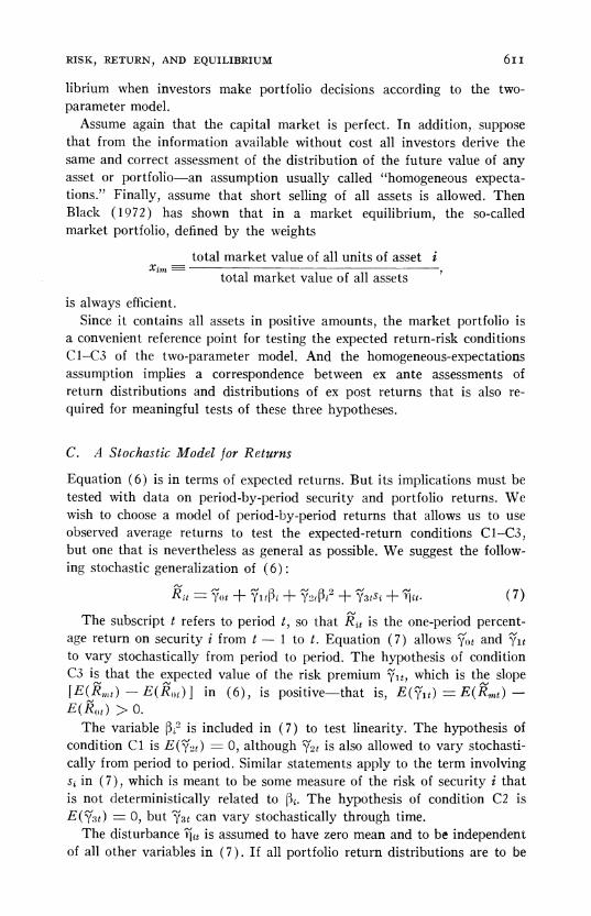
Testing the two-parameter model immediately presents an unavoidable "errors-in-the-variables" problem: The efficiency condition or expected return-risk equation (6) is in terms of true values of the relative risk measure p,, but in empirical tests estimates, b,, must be used. In this paper

-Awhere cov(R,, k,,,)and ~ ' ( k , , , ) are estimates of cov(k, , #,,,) and ~ " k , , , ) A,

obtained from monthly returns, and where the prosy chosen for Rn,t is "Fisher's Arithmetic Index," an equally weighted average of the returns on all stocks listed on the S e w York Stock Exchange in month t . The properties of this index are analyzed in Fisher (1966).

Blurne (1970) shows that for any portfolio p, defined by the weights x L p , i = l , 2 , . . . ,x,


If the errors in the p, are substantially less than perfectly positively cor- *elated, the p's of portfolios can be much more precise estimates of true

A

(3's than the 13's for individual securities. T o reduce the loss of information in the risk-return tests caused by

using por t fops rather than individual securities, a wide range of values of portfolio P,'s is obtained by forming portfolios on the basis of ranked

A

values of 13, for individual securities. But such a procedure, nai'vely exe-cuted could result i t a serious regression phenomenon. I n a cross section of p,,high observed 13, tend to be above the correspondin? true fitand low observed 1,tend to be below the true (3,. Forming portfolios on the basis

A

of ranked p, thus causes bunching of positive and negative sampling errors within portfolios. The result is that a large portfolio D, would tend to over- state the true p,, while a low t, would tend to be an underestimate.

The regression phenomenon can be avoided to a large extent by forming A

portfolios from ranked 13, computed from data for one time period but then using a subsequent period to obtain the 8, for these portfolios that are used to test the two-parameter model K i t h fresh data, within a portfolio errors in the individual security

AP, are to a large extent random across securities, so that in a portfolio 6,the effects of the regression phenomenon are, it is hoped, minimized."

The specifics of the approach are as follows. Let S be the total number of securities to be allocated to portfolios and let int(hT/20) be the largest integer equal to or less than X 20 Using the first 4 years (1926-29) of monthly return data, 20 portfolios are formed on the basis of ranked p, for individual securities. The middle I d portfolios each has in t (S /20) securities If S is even, the tirst and last portfolios each has int(ill"20) +

IS 20 int(iV 20) ] securities. The last (highest B ) portfolio gets an-

additional security if X is odd. The follou,ing 5 years (1930-34) of data are then used to recompute

the p,, and these are averaged across securities within portfolios to obtain 20 initial portfolio b,,! for the risk-return tests. The subscript t is added to indicate that each month f of the follo~ving four years (1932-38) theseB,, ale recomputed as simple averages of individual security P,, thus ad- justing the portfolio ii',,, month by month to allon for delisting of securities. The component b, for securities are themselves updated yearly-that

'; Thc errors-in-the-v:iri:~l)les problem and the teclinique of using portfolios to sol\.e it were iirst pointed out by Blume (1970). The portiolio approach is also used by Friend and Blume (1970) and Black, Jensen, and Scholes (1972). The regression phenomenon that arises in risk-return tcsts xvas first recognized by Blumc (1970) and then by Black, Jensen, and Scholes ( 1 9 i i ) , who offer a solution to the prol~lem that is similar in spirit to ours.


is, they are recomputed from monthly returns for 1930 through 1935, 1936, or 1937.

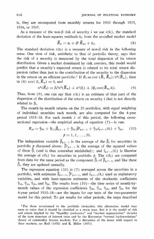
As a measure of the non-/$ risk of security i we use s(2,), the standard deviation of the least-squares residuals ?,t from the so-called market model

g,t= +qt.a, + /3GTnt (8)

The standard deviation s(?,) is a measure of non-p risk in the following sense. One view of risk, antithetic to that of portfolio theory, says that the risk of a security is measured by the total dispersion of its return distribution. Given a market dominated by risk averters, this model would predict that a security's expected return is related to its total return dispersion rather than just to the contribution of the security to the dispersion in the return on an efficient portfolio.' If B, -cov (EL, R,,,)/cs2(ErN),then

,-"in (8 ) cov( Zt, R,,) = 0, and

?d

cs2(RL)= 2/31 C O V ( E ~ , , (9~ t '~ ' (En l )+ o'(?{) + rb) .

Thus, from ( 9 ) , one can say that s(?,) is an estimate of that part of the dispersion of the distribution of the return on security i that is not directly related to /3,.

The month-by-month returns on the 20 portfolios, with equal weighting of individual securities each month, are also computed for the 4-year period 1935-38. For each month t of this period, the following cross-sectional regression-the empirical analog of equation (7)-is run:

Rpt =90t+ v l t p p , t - 1 + ??t p2, t - l + ??I% t-I(?,) + ? p + , ( l o )

p = 1 , 2 , . . . , 20.

The independent variable p, t _ l is the average of the p, for securities in portfolio p discussed above, n2, t _ l is the average of the squared values of these p, (and is thus somewhat mislabeled) ; and , - I (2,) is likewise the average of s(?,) for securities in portfolio p. The s(2,) are computed from data for the same period as the component p, of f?~,,~ and like these P,, they are updated annually.

The regression e q u a t i o ~ (10) is ( 7 ) averaged across the securities in a portfolio, with estimates 13, t - , . b'p t - l , and T, (2,) used as explanatory variables, and with least-squares estimates of the stochastic coefficients 9ot, 91t, y ~ t ,and The results from (10)-the time series of month-by- month values of the regression coefficients Pot, Tit, 3 r t , and ?St for the 4-year period 1935-38-are the inputs for our tests of the two-parameter model for this period. To get results for other periods, the steps described

7For those accustomed to the portfolio viewpoint, this alternative model may seem so nai've that it should be classified as a straw man. But it is the model of risk and return implied by the "licluidity preference" and "market segmentation" theories of the term structure of interest rates and by the Keynesian "normal backv,,ardation" theory of commodity futures markets. For a discussion of the issues with respect to these markets, see Roll (1970) and K. Miller (1971).


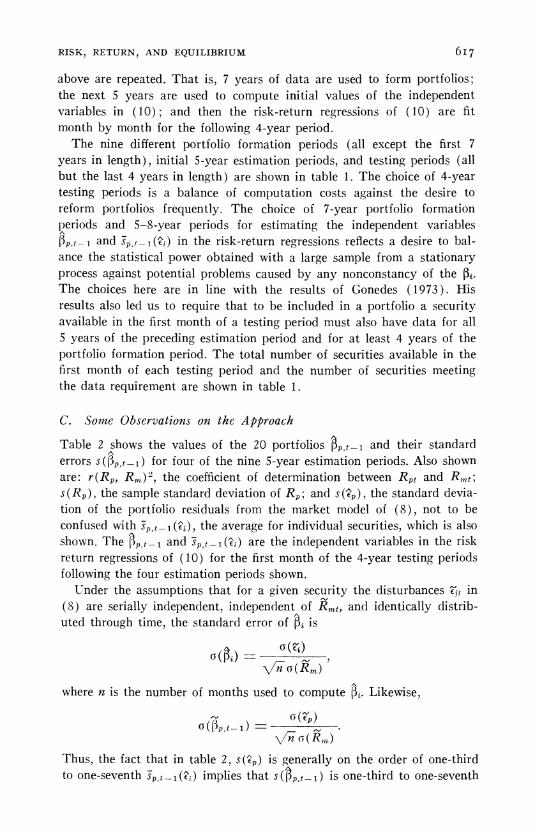
above are repeated. That is, 7 years of data are used to form portfolios: the nevt 5 years are used to compute initial values of the independent variables in ( 1 0 ) ; and then the risk-return regressions of (10) are fit month by month for the follotving 4-year period.

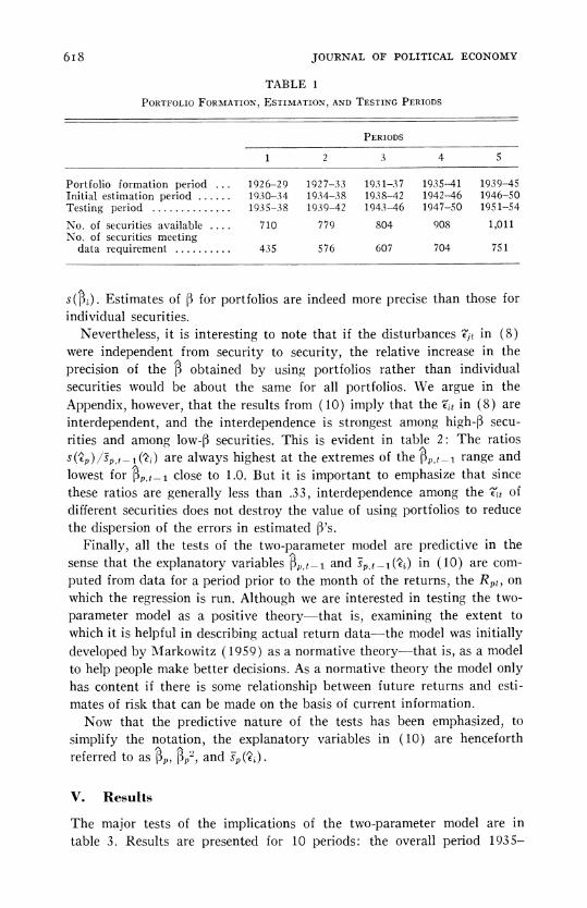
The nine different portfolio formation periods (all except the first 7 years in length), initial 5-year estimation periods, and testing periods (all but the last 4 years in length) are shown in table 1. The choice of 4-year testing periods is a balance of computation costs against the desire to reform portfolios frequently. The choice of 7-year portfolio formation periods and 5-8-year periods for estimating the independent variables BP t - 1 and S,] + - I (2,) in the risk-return regressions reflects a desire to balance the statistical power obtained with a large sample from a stationary process against potential problems caused by any nonconstancy of the p,. The choices here are in line with the results of Gonedes (1973). His results also led us to require that to be included in a portfolio a security available in the first month of a testing period must also have data for all 5 years of the preceding estimation period and for a t least 4 years of the portfolio formation period. The total number of securities available in the first month of each testing period and the number of securities meeting the data requirement are shown in table 1.

C. Some Observations on the Approach

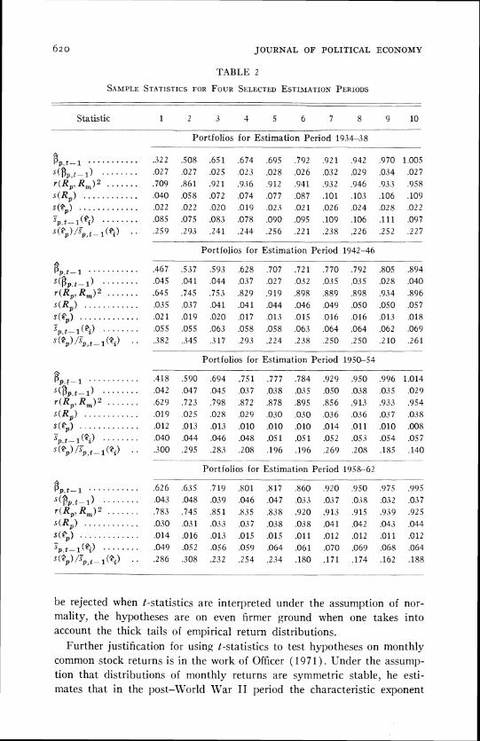
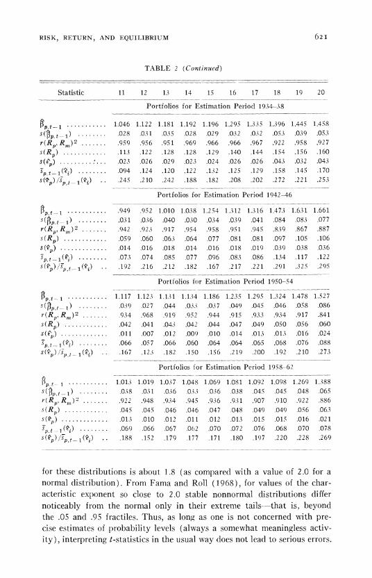
Table 2 shows the values of the 20 portfolios 6,t - l and their standard errors s(P, t - l ) for four of the nine 5-year estimation periods. Also shown are: r(R,, R,,,)', the coefficient of determination between Rilt and R,,,t; s (R , ) , the sample standard deviation of R,: and s(2,), the standard deviation of the portfolio residuals from the market model of ( 8 ) , not to be confused nith F,t p l (2 , ) , the average for individual securities, nhich is also shown. The jlf, and S, ,-,(2,) are the independent variables in the risk return regressions of (10) for the tirst month of the 4-year testing periods following the four estimation periods shonn.

Under the assumptions that for a given security the disturbances in (8) are serially independent, independent of and identically distributed through time, the standard error of b, is

where n is the number of months used to compute b,. Likewise,

Thus, the fact that in table 2 , s(2,) is generally on the order of one-third to one-seventh S;,t-l(i',) implies that s ( f iPJ tp l ) is one-third to one-seventh


TABLE 1

PoKTIOLTO FORAZ~ZTIOS, AND TLSTTNC~ S T T A Z ~ T I O N , PERIODS

PERIODS

Portfolio formation period . . . 1926-29 1917-3.3 1931-37 1935-41 1939-45 Ir~itinl estimation period . . . . . . 19.<0-34 1904-38 1938-42 1942-46 1946-50 Testing period . . . . . . . . . . . . . . 1935-38 1939-42 1943-46 1947-50 1951-54

No. of securities available . . . . 710 779 804 908 1,011 No, of securities meeting

data requirement . . . . . . . . . . 40.5 576 607 704 75 1

~(3,).Estimates of /3 for portfolios are indeed more precise than those for individual securities.

Kevertheless, it is interesting to note that if the disturl~ances 't;, in (8) were independent from security to security, the relative increase in the precision of the fi obtained by using portfolios rather than individual securities would be about the same for all portfolios. \Ye argue in the Appendix, however, that the results from (10) imply that the ';l,t in (8) are interdependent, and the interdependence is strongest among high-P secu-rities and among low-p securities. This is evident in tabie 2 : The ratios ~(2, ) )Sg t - (2 , ) are always highest a t the extremes of the P, range and lowest for 8, close to 1.0. But it is important to emphasize that since these ratios are generally less than 3 3 , interdependence among the Zt of different securities does not destroy the value of using portfolios to reduce the dispersion of the errors in estimated p's.

Finally, all the tests of the two-parameter model are predictive in the A

sense that the explanatory variables P, t - l and S, t-l(Q,) in (10) are computed from data for a period prior to the month of the returns, the R,(, on which the regression is run. Although we are interested in testing the two- parameter model as a positive theory-that is, examining the extent to which it is helpful in describing actual return data-the model was initially developed by Jfarkowitz ( 1959) as a normative theory-that is, as a model to help people make better decisions. As a normative theory the model only has content if there is some relationship between future returns and estimates of risk that can be made on the basis of current information.

Now that the predictive nature of the tests has been emphasized, to simplify the notation, the explanatory variables in (10) are henceforth referred to as p,, $,', and G ( 2 , ) .

V. Results

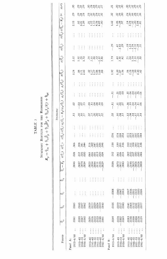
The major tests of the implications of the two-parameter model are in table 3. Results are presented for 10 periods: the overall period 1935-

RISK, RETURN, AND EQUILIBRIUlM 619

TABLE 1 (Continlied)

PERIODS

Portfolio formation period . . . 1943-49 1947-53 19.51-57 195.5-61 Initial estimation period . . . . . . 1950-54 19.54-58 1958-62 1962-66 Testing period . . . . . . . . . . . . . . 1955-58 1959-62 1963-66 1967-68

No. of securities available . . . . 1,053 1,065 1,162 1,261 S o . of securities meeting

data requirement . . . . . . . . . . 802 856 8.58 845

6 '68; three long subperiods, 1935-45, 1946-55, and 1956-6/68; and six subperiods which, except for the first and last, cover 5 years each. This choice of subperiods reflects the desire to keep separate the pre- and post- LVorld n-ar I1 periods. Results are presented for four different versions of the risk-return regression equation ( 10) : Panel D is based on ( 10) itself, but in panels A-C, one or more of the varkbles in (10) is suppressed. For each period and model, the table shows: T,, the average of the month- by-month regression coefficient estimates, ?,, ; s(?,) , the standard deviation of the monthly estimates: and 7' and s(Y'", the mean and standard deviation of the month-by-month coefficients of determination, ri" which are adjusted for degrees of freedom. The table also shows the first-order serial correlations of the various monthly computed either about the sample mean of y,, [in which case the serial correlations are labeled p11(?,) 1 or about an assumed mean of zero [in which case they are labeled p ~ ( ? , )1 . Finally, t-statistics for testing the hypothesis that 9, =0 are presented. These t-statistics are

-

where 12 is the number of months -in the period, which is also the number of estimates q,t used to compute Q, and s(?,) .

In interpreting these t-statistics one should keep in mind the evidence of Fama ( 1 9 6 5 ~ ) and Blume (1970) which suggests that distributions of common stock returns are "thick-tailed" relative to the normal distribution and probably conform better to nonnormal symmetric stable distributions than to the normal. From Fama and Babiak (1968)) this evidence means that when one interprets large t-statistics under the assumption that the underlying variables are normal, the probability or significance levels obtained are likely to be overestimates. But it is important to note that, with the exception of condition C3 (positive expected return-risk tradeoff), upward-biased probability levels lead to biases toward rejkction of the hypotheses of the two-parameter model. Thus, if these hypotheses cannot

-- - - - -- - -


Statistic 1 2 3 4 5 6 7 8 9 1 0 - -.---

Portfolios for Estimation Period 1934-38

Portfolios for Estimation Period 1942-46

Portfolios for Estimation Period 1950-54 h

f l p , t - l . . . . . . . . . . . ,418 ,590 ,694 ,751 ,777 ,784 .929 ,950 ,996 1.014

s ($ , , , _ , ) . . . . . . . . ,042 ,047 ,045 ,067 .038 ,035 ,050 ,038 ,035 .029 r(R, . R,,)? . . . . . . ,629 ,726 ,798 372 3 7 8 ,895 ,856 ,913 ,933 ,954 s ( R P ) . . . . . . . . . . . . ,019 ,025 ,028 ,029 ,030 ,030 .0.36 .0.36 ,037 .0.38 s ( F ) . . . . . . . . . . . . . ,012 .013 ,013 ,010 .010 ,010 ,014 ,011 ,010 ,008 S P , , - 6 . . . . . . . . ,040 ,044 ,046 ,048 .051 ,051 ,052 ,053 ,054 ,057 s ? ~ ! ~ , ~ ? ~ ). . ,300 ,295 ,283 ,208 ,196 .I96 ,269 ,208 .185 ,140

..-

Portfolios for Estimation Period 19.78-62

B p , , - . . . . . . . . . . . ,626 ,635 ,719 .SO1 ,817 860 920 ,950 ,975 ,995 s ( t P,,-,) . . . . . . . . .04.3 ,048 ,039 ,046 ,047 0 3 ,037 .O.W .0.32 ,037 r ( R p , R,,)? . . . . . . ,783 ,745 ,851 ,835 838 ,920 .91d .915 ,939 ,925 s ( R p ) . . . . . . . . . . . . ,030 ,031 .O.<.i ,037 ,038 ,038 ,041 ,042 ,043 ,044 s ( $ ) . . . . . . . . . . . . . ,014 ,016 ,013 .015 .015 .011 .012 ,012 ,011 ,012 S p , t - l ( @ i ) . . . . . . . . ,049 ,052 .056 .059 ,064 ,061 ,070 ,069 .068 ,064 s ~ / ~ . . , ~ ,308 ) ,254 2.14 ,180 ,171 ,174 ,162,286 ~ ,232 ,188

be rejected when t-statistics are interpreted under the assumption of nor-mality, the hypotheses are on even firmer ground when one takes into account the thick tails of empirical return distributions.

Further justification for using t-statistics to test hypotheses on monthly common stock returns is in the work of Officer ( 1971 ) . Cnder the assumption that distributions of monthly returns are synimetric stable, he estimates that in the post-Korld War I1 period the characteristic exponent

--

----

RISK, RETURN, AND EQUILIBRIUM 62 I

T;\BLE 2 (Cotz t in f tcd)

Statistic 11 12 13 14 15 16 17 18 10 20 ------- ------ -- -- .

Portfolios for Estimation Period 1934-38 -

8 . . . . . . . . . . . 1.046 1.122 1.181 1.192 1.106 1.29.i 1.3.35 1.196 1.445 1.458

s(B,,,-- ,) . . . . . . . . .028 .0,11 ,035 ,028 ,029 ,032 ,032 ,053 .0,39 ,053

v(R,]. I?,,,)' . . . . . . . 9 ,956 .95 1 ,969 ,066 ,966 ,967 ,022 ,958 ,927

s (R ) . . . . . . . . . . . . 1 ,122 ,128 ,128 ,129 ,140 154 ,153 ,156 ,160

s ( E ) . . . . . . . . . :. . . ,023 ,026 ,029 ,023 ,024 ,026 ,026 ,043 ,032 ,043

S,,t- , (2,) . . . . . . . . ,094 ,123 ,120 1 2 2 .I.{? ,125 1 2 .1.58 1 ,170

s ' l J , t ,( € 1 . . ,235 ,210 ,232 ,188 ,182 ,208 ,202 ,272 ,221 ,253 -pp-p--p- - - - - -

Portiolios ior Estimation Period 1942-36 - - . --a,,, I . . . . . . . . . . . ,049 ,952 1.010 1.038 1.253 1.112 1.316 1.473 1.631 1.661

s ( P p - 1 ) . . . . . . . . ,031 O.i6 ,030 ,030 ,034 .0.39 ,051 ,084 ,083 ,077 riRI,. R,,,)? . . . . . . ,942 ,923 ,917 ,054 ,958 .9.51 ,935 ,839 ,867 ,887 S(R,) . . . . . . . . . . . . ,059 ,060 ,063 ,064 ,077 ,081 ,081 ,097 ,105 ,106 ~ ( 9 ~ ). . . . . . . . . . . . . ,014 0 1 6 ,018 ,014 ,016 ,018 ,010 ,030 ,038 .036

T,,, ( P i ) . . . . . . . . ,073 ,074 085 ,077 ,096 ,083 ,086 ,133 ,117 ,122

S , . . ,192 ,216 ,212 ,182 ,167 ,217 ,221 ,291 .32' ,295 - - - - - -~

Portiolios ir~r Estimation Period 1950-?4 .. - . -

f i , , t - l . . . . . . . . . . . 1.117 l.12.i 1.1.11 1.1.34 1.186 1.235 1295 l..124 1478 1.527

s ( f i , , , ) . . . . . . . . .0.30 ,027 ,034 .O.l.i ,037 ,040 ,035 ,046 ,058 ,086 ?'(R,. R,,,)? . . . . . . .0.34 ,968 ,919 ,951 ,943 ,915 .03.3 ,034 ,017 ,841 s(R,) . . . . . . . . . . . . ,042 041 .04.i ,042 ,045 ,047 ,049 ,050 ,056 ,060 s($) . . . . . . . . . . . . ,011 ,007 ,012 ,004 ,010 ,013 ,013 .Ol.1 ,016 ,024

SI,. - ( P i ) . . . . . . . . ,066 . 0 5 ,066 060 ,064 ,064 ,065 ,068 ,076 ,088 ? ., ) . . ,167 . I > . ? ,182 ,150 ,156 2 1 9 200 ,192 ,210 ,273

------.- .- - .-.- -- -- - - - -.---Portiolios ior Estimation Period 19.58-62

~.~

fl,, , . . . . . . . . . . . 1.013 1019 1.037 1.048 1.069 1.081 1.002 1.008 1.269 1..388 ~ ( f i ~ , ~ - -. . . . . . . . .0.18 ,031 .O.i6 .Oii .O.i6 ,038 ,045 ,035 ,048 .O6il )

r(R,,. R,,,)" . . . . . . . ,922 ,948 .0.14 ,045 ,936 .0.i1 ,907 ,910 ,922 ,886

s(R,,) . . . . . . . . . . . . .045 ,045 ,056 ,036 ,047 ,048 ,049 059 ,056 .O6.1 ~(3,). . . . . . . . . . . . . .Ol.i 010 ,012 ,011 ,012 ,013 ,015 ,015 ,016 ,021

.?/, (0 , ) . . . . . . . . ,069 ,066 ,067 ,002 ,070 ,072 ,076 ,068 ,070 ,078 s ' , . . 188 ,152 1 7 ,177 1 1 ,180 ,107 220 ,228 ,269

for these distributions is about 1.8 (as compared with a value of 2.0 for a normal distribution). From Fama and Roll ( 1968), for values of the characteristic exponent so close to 2.0 stable nonnormal distributions differ noticeably from the normal only in their extreme tails-that is, beyond the .05 and .95 fractiles. Thus, as long as one is not concerned with precise estimates of probability levels (always a somewhat nieaningless activ- i ty) , interpreting t-statistics in the usual way does not lead to serious errors.

3. O O N e l S O - i D 0

8 E:: ::$f:g9 909 999999

0 U W N - 3 0 1 0 m e N b 3 N " 0 0 S i i - e- 1 9 1 - . 1 1 9 9 :

'n * N i r N N " h 3 W" C b W - D b W b h 9 - 9 9 199999

. . . . . . . . . . . . . . . . . . . . . . . . . . . . . . m m m m i .0 W a

0 " 0 1 0 0 \ 5 "LO, O lnO"O\ ee l r lO.0 .0 .0 f " U b e " m 0 . O

I ? ? I A A$& J , l & A A Lm-L , - i -r e f ln"U - - - * l o - i b b " r n W s m 3 3 3 m-*---- i. 3 30;. m m n ~ m m - ... --- ------

*


Inferences based on approximate normality are on even safer ground if one assumes, again in line with the results of Officer (1971), that although they are well approximated by stable nonnormal distributions with u r 1.8, distributions of monthly returns in fact have finite variances and converge- but very slowly-toward the normal as one takes sums or averages of individual returns. Then the distributions of the means of month-by-month regression coefficients from the risk-return model are likely to be close to normal since each mean is based on coefficients for many months.

A. Tests of the Major Hypotheses of the Two-Parameter Model

Consider first condition C2 of the two-parameter model, which says that no measure of risk, in addition to (3, systematically affects expected returns. This hypothesis is not rejected by the results in panels C and D of table 3. The values of t(F3) are small, and the signs of the t ( 9 , ) are randomly positive and negative.

Likewise, the results in panels B and D of table 3 do not reject condition C1 of the two-parameter model, which says that the relationship between expected return and @ is linear. In panel B, the value of t(?-) for the overall period 1935-6/68 is only -.29. In the 5-year subperiods, t(72) for 1951-55 is approximately -2.7, but for subperiods that do not cover 1951-55, the values of t (T2) are much closer to zero.

So far, then, the two-parameter model seems to be standing up well to the data. All is for naught, however, if the critical condition C3 is rejected. That is, we are not happy with the model unless there is on average a positive tradeoff between risk and return. This seems to be the case. For the overall period 1935-6/68, t ( q l ) is large for all models. Except for the period 1956-60, the values of t ( 9 , ) are also systematically positive in the subperiods, but not so systematically large.

The small t-statistics for subperiods reflect the substantial month-to- month variability of the parameters of the risk-return regressions. For example, in the one-variable regressions summarized in panel A, for the period 1935-40, i)l = .0109. I n other words, for this period the average incremental return per unit of (3 was almost 1.1 percent per month, so that on average, bearing risk had substantial rewards. Kevertheless, because of the variability of qlt-in this period s ( q l ) is 11.6 percent per month ( ' )-t(q1) is only .79. I t takes the statistical power of the large sample for the overall period before values of that are large in practical terms also yield large t-values.

But a t least with the sample of the overall period t (q l ) achieves values supportive of the conclusion that on average there is a statistically observable positive relationship between return and risk. This is not the case with respect to ~ ( $ 1 ) and t ( q 3 ) .Even, or indeed especially, for the overall period, these t-statistics are close to zero.

RISK. RETURN, AND rQUILIBRIVM 6 2 j

The behavior through time of 31:,and is also consistent with hypothesis hlE that the capital market is efficient. The serial correlations p li(:'l). p , , ( ~ , ) . and ,) , are always low in terms of explanatory power and generally low in terms of statistical significance. The proportion of the variance of ?,+explained by first-order serial correlation is estimated by p(3,) ' which in all cases is small. As for statistical significance, under the hypothesis that the true serial correlation is zero, the standard deviation of the sample coefficient can be approximated by n($) = I/$. For the overall period, ri(p) is approximately 05, while for the 10- and 5-year subperiods o ($) is approximately .09 and .13, respectively. Thus, the values of p,r(q,), p , , ( ~ ~ ) . and pr,(T+) in table 3 are generally statistically close to zero. The exceptions involve primarily periods that include the 193.5-30 subperiod, and the results for these periods are not independent.'

To conserve space, the serial correlations of the portfolio residuals, q p t ,

are not shown In these serial correlations, negative values predominate. But like the serial correlations of the ?'s, those of the q's are close to zero. Hiqher-order serial correlations of the ?'s and 'lj's have been computed, and these also are never systen~atically large.

In short, one cannot reject the hypothesis that the pricing of securities is in line with the implications of the two-parameter model for expected returns. And given a two-parameter pricing model, the behavior of returns through time is consistent with an efficient capital market.

B . Thr, Bchavior oj thr Markct

Some perspective on the behavior of the market during different periods and on the interpretation of the coefficients and in the risk-return regressions can be obtained from table 1.For the various periods of table 3, table 3 shows the sample means (and with some exceptions), the standard

" T h e sizri;il correlations o i 9, and Q:l about means that are assumed to be zc,ro provide a test of the fair game property of an efficient market. given that eapc,cted returns are generated by the t~vo-parameter model- -that is, givcn E ( y , , ) =E(?:, , ) =0. Likewise, p,,(Q,,, -R,,) provides a test of market efficiency with respect to the beha\-ior o i Q , , , thr0ut.h time, given the validity of thc Sharpc-Lintner hypothesis iabout which we have as yet said nothing) . But , a t least for and q:,,,computinr the serial correlations about sample means produces essentially the _same results.

T o test thc market eficiency hypothesis - on Tlt -w

[EiR,,,,)- E(R,,,)I , the sample mean of the 9,:is used to estimate E(R,,,,)- E(R,, ,) .thus implicitly assuming that the expected risk premium is constant. T h a t this is a reasonable approximation lin the-sense that,"the p , , ( Q , ) are smalll. pro1)al)ly reflects the iact that variation in E(R,,,,)- E:'(R,,:)is trivial relative to the month-by-month \-ariation in Q,,.

Finally, it is well to note that in terms of the implications of the serial correl:~tions for making good portfolio decisions-and thus ior judging whether market efficiency is a workal~le representation of reality-the iact tha t the 'serial corl-elations are low in terms of explanatory power is more important than whether or not they are lo\v in terms of statistical significance.

JOURNAL O F POLITICAL ECONOMY

TABLE 4

*Since s ( R r ) is so sinall relative to s(R,,). s(R,,, - X I ) . which is not shown, is essentially the same sil?, ,L).The standard de\-iations of (K,,, - Rr) / s (R , , , ) and $,.'s(R,,,), also not shown. can he

obtnked directly from s(R,,, -K T ) ,s ( $ ~ )and s(K nj) . E n a l l y , the t-statistics for (R,,,- Rf) , ' s (R, , ) and Q,i's(R,,) are irlentical with those lor R,,, -R , and 9,.

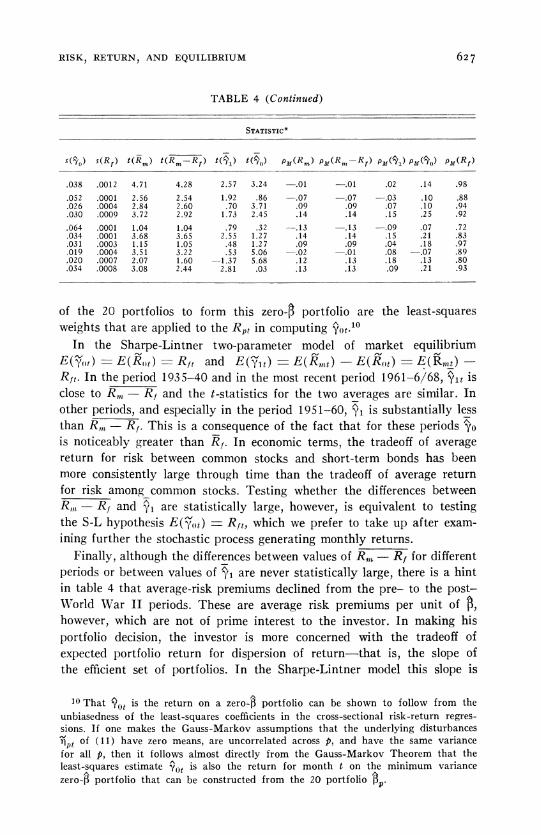
deviations, t-statistics for sample means. and first-order serial correlations for the month-by-month values of the following variables and coefficients: the market return R,,,,; the riskless rate of interest Rit, taken to be the yield on I-month Treasury bills; RlIlt-R f t ; (Rrnt - R,t) s(R,,,) : 9 0 t

and repeated from panel -4 of table 3 : and q i t / ~ ( R , , , ) .The t-statistics on sample means are computed in the same way as those in table 3 .

If the tno-parameter model is valiti, then in equation ( 7 ) , B(y0t)= ~ ( i i , , , ) , on orwhere I?(&) is the expected return any zero-p security portfolio. Likewise, the expected risk premium per unit of P is B(Ernt)--.,E(R, , t )=E(7lt) . In fact, for the one-variable regressions of panel A, table 3 , that is,

Rpt = 90t + 91t b p + ? p i , ( I I 1 we have, period by period,

This condition is obtained by averaging ( 1 1 ) over p and making use of the least-squares constraint

c .;I,, = 0.:) P

hloreover, the least-squares estimate can always be interpreted as the return for month t on a zero$ portfolio, where the weights given to each

!'There is some degree of approximation in ( 1 2 ) . The averages over P of R,, and fir, arc R,,,,and 1.0, respectivcly, only if every security in the market is in some portfolio. CVith our methodology (see table 1) this is never true. But the degree of approximation turns out to he small: The average o i the R,,, is always close to R,,,t and the average a,, is always close to 1.0.

RISK, RETURN, AND EQUILIBRIUM b27

TABLE 4 (Continued)

STATISTIC*

of the 20 portfolios to form this zero$ portfolio are the least-squares weights that are applied to the RPtin computing (Iot.lo

In the Sharpe-Lintner two-parameter model of market equilibrium ,-d N

E(yot)=E ( E ( , ~ )= Rit and E(y l t )=E(E,t) -E(Rot)=E(R+) -Rft. In the period 1935-40 and in the most recent period 1961-6/68, ^yl t is close to R,,,-- R, and the t-statistics for the two averages are similar. In other periods, and especially in the period 1951-60, "y is substantially less than R, -Ri. This is a consequence of the fact that for these periods 70 is noticeably greater than ?Ti.In economic terms, the tradeoff of average return for risk between common stocks and short-term bonds has been more consistently large through time than the tradeoff of average return for risk among common stocks. Testing whether the differences between R,,,- Ri and jl are statistically large, however, is equivalent to testing the S-L hypothesis E('j;, ,)= Rit, which we prefer to take up after examining further the stochastic process generating monthly returns.

Finally, although the differences between values of R, -Rffor different periods or between values of 7, are never statistically large, there is a hint in table 4 that average-risk premiums declined from the pre- to the post- IVorld War I1 periods. These are average risk premiums per unit of fj, however, which are not of prime interest to the investor. In making his portfolio decision, the investor is more concerned with the tradeoff of expected portfolio return for dispersion of return-that is, the slope of the efficient set of portfolios. In the Sharpe-Lintner model this slope is

1 0 That 9,,t is the return on a zero-8 portfolio can be shown to follow from the unbiasedness of the least-squares coefficients in the cross-sectional risk-return regres-sions. If one makes the Gauss-Markov assumptions that the underlying disturbances ,"~ 1 , ~of (11) have zero means, are uncorrelated across p, and have the same variance for all p, then it follows almost directly from the Gauss-Markov Theorem that the least-squares estimate Qot is also the return for month t on the minimum variance zero$ portfolio that can be constructed from the 2 0 portfolio Bg.


,-d

always [E(R,,t) - R f t ] / ~ ( g , , , , ) ,and in the more general model of Black (1972)) it is [ E ( E , ~ , ) -E ( & ) ] / G ( E , ~ , )at the point on the efficient set corresponding to the market portfolio m.-I n table 4, especially for the three long subperiods, dividing R,,, - Rf and T I , by s(R,,,) seems to yield estimated risk premiums that are more constant through time. This results from the fact that any declines in or R,, -Rf are matched by a quite noticeable downward shift in s(R,),) from the early to the later periods (cf. Blume [I9701 or Officer 119711).

C. Errors and True Variation in the Coe@cients 9,t

Each cross-sectional regressim coefficient Vlt in (10) has two components: ,-dthe true 7,t and the estimation error, = - ylt. A natural question

is: To what extent is the variation in qlt through time due to variation in y,, and to nhat extent is it due to Tit? In addition to providing important information about the precision of the coefficient estimates used to test the two-parameter model, the answer to this question can be used to test hypotheses about the stochastic process generating returns. For example. although we cannot reject the hypothesis that E(Ylt) = 0, does including the term involving P,' in (10) help in explaining the month-by-month behavior of returns? That is, can we reject the hypothesis that for all t , ,.,y ~ t= O? Likewise, can we reject the hypothesis that month-by-month 71,= O ? And is the variation through time in But due entirely to Tot and to variation in R f t ?

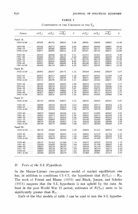
The answers to these questions are in table 5 . For the models and time periods of table 3, table 5 shows for each 9 , : sq(P,), the sample variance of the month-by-month i j,,; s2(T,) , the average of the month-by-month values of s"ylt), \\here s (TI t ) is the standard error of 3,!from the cross-

Asectional risk-return regression of ( 1 0 ) x m o n t h t ; s2(y1)= ~ ' ( y , )-s2(?,) ; and the F-statistic F = s"(y ,) /s2($,), which is relevant for testing the hypothesis, s"(::,) = s2($,). The numerator of F has n - 1 df, where n is the number of months in the sample period, and the denominator has n(20 - K ) df, where K is the number of coefficients 9, in the model."

11 The standard error of Q,,, s($,,), is proportional to the standard error of the risk-return residuals, 3 for month t , which has 20 -K df. And n values of s'($,,)

-7%-are avetaged to get s-(Q,) , so that the latter has n(20 - K ) df. Kote that if the underlying return disturbances T,, of (10) are independent across p and have identical

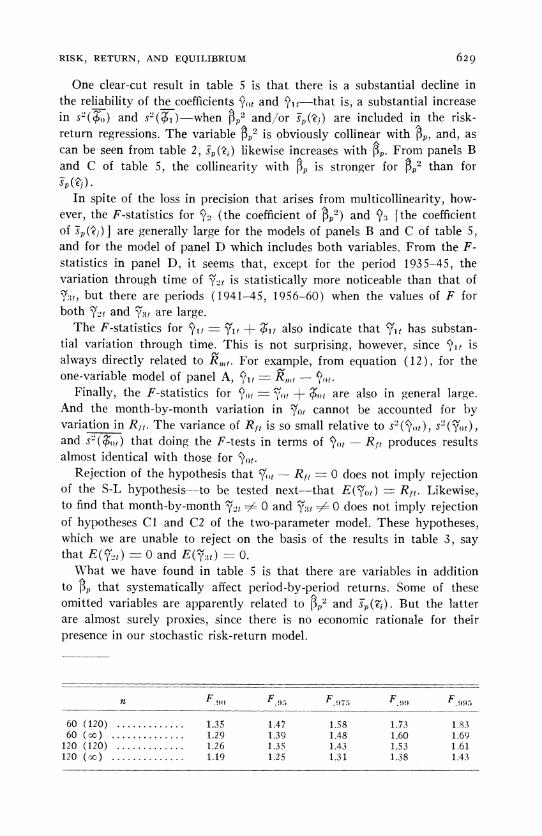
e -normal distributions for all p, then Qi t is the sample mean of a normal distvibution and sV&,,) is proportional to the sample variance of the same normal distribution. If the p r o c e s s ~ l s o assumed to be stationary through time, it then follows that s2(?,,) and s'"(Fit) are independent, as required by the F-test. Finally, in the F-statistics of table 5 , the values of n are 60 or larger, so that, since K is irom ? to 4, n (20- K ) 2 960. From Mood and Graybill (1963), some upper percentage points of the F-distribution are:

RISK, RETURN, AKD EQUILIBRIUM 629

One clear-cut result in table 5 is that there is a substantial decline in the reliability of the coefficients q,,,and ?],-that is, a substantial increase in s2(K)and s2(K)--when p,' and /or Q(Qi )are included in the risk- return reqressions. The variable p,' is obviously collinear with &,: and, as

A

can be seen from table 2 , S,(?,) likewise increases with PI,. From panels B and C of table 5, the collinearity with P, is stronger for P,"han for

GiG). In spite of the loss in precision that arises from multicollinearity, how-

ever, the F-statistics for qy ( the coefficient of b,') and ?:{ (the coefficient of S , ( Q i ) ] are generally large for the models of panels B and C of table 5, and for the model of panel D which includes both variables. From the F-statistics in panel D, it seems that, except for the period 1935-45, the variation through time of y2i is statistically more noticeable than that of y:;t, but there are periods ( 1941-45, 1956-60) when the values of F for both 72,and ?:(,are large.

The F-statistics for Q l 1 = +$,+also indicate that vithas substantial variation through time. This is not surprising. however, since fit is always directly related to K,,,,.For example. from equation (12) , for the

.-,one-variable model of panel A, q l , = R,,,,-?,,,.

Finally, the F-statistics for = y,,,+ &,+are also in general large. And the month-by-month variation in ;;i'rrl cannot be accounted for by variation in R,,. The variance of Rit is so small relative to s"?,,,), s ' ( ~ , ~ , , , and s"$ , , I ) that doing the F-tests in terms of - K i t produces results almost identical with those for 3,,t.

Rejection of the hypothesis that c,, -- K,, :z 0 does not imply rejection of the S-L hypothesis --to be tested nest---that E ( v , , , )- Rf, . IJikewise, to find that month-by-month 7,: =# 0 and y:{r+0 does not imply rejection of hypotheses C1 and C2 of the two-parameter model. These hypotheses, which me are unable to reject on the basis of the results in table 3 , say that E ( Y 2 [ )= 0 and E(';;:,,)= 0.

[That we have found in table 5 is that there are variables in addition to p, that systematically affect period-by-period returns. Some of these

A

omitted variables are apparently related to p,,%nd c(Ti).Rut the latter are almost surely proxies, since there is no economic rationale for their presence in our stochastic risk-return model.

JOURNAL O F POLITICAL ECONOMY

TABLE 5

I'FRIOU

I'anel A: 1935-6168 . . .

s o )

,00105

s?(q,))

,00142

-s ,

,00037

F

3.84

~ ~ ( 7 , )s

,00401 .00436

-S )

,00035

F

12.46

I'anel B: 1935-6168 . . . ,00092 ,00267 .00175 1.52 ,00564 ,01403 ,00839 1.67

Panel C: 1935-6168 . . . ,00192 ,00266 ,00075 3.55 ,00285 ,00428 ,00142 3.01

I'anel D: 1935-6/68 . . . ,00150 ,00566 00406 1.39 ,00608 ,01521 ,00913 1.66

D. Tests of the S-L Hypothesis

In the Sharpe-Lintner two-parameter model of market equilibrium one has. in addition to conditions ClLC3, the hypothesis that E ( y , , t )= Rrt. The work of Friend and Blume (1970) and Black, Jensen, and Scholes (1972) sucgests that the S-L hypothesis is not upheld by the data. At least in the post-IYorld IYar I1 period, estimates of E(y,,t)seem to be siqnificantly creater than Rft .

Each of the fdur models of table 3 can be used to test the S-L hypothe-


T.4BLE 5 (Continued)

I'anel A : 1935-6/68

1 9 3 5 4 0 . . . . . 1 9 4 1 4 5 . . . 1946-50 . . . . 1951-55 . . . 1956-60 . . . . . 1961-6/68 . . .

Panel B : 1935-6168 . . .

I'anel C: 1935-6168

Panel D: 1935-6/68 . . . .00061 ,00362 ,00301 1.21 ,276 ,864 ,588 1.47

s i s . l T h e most efficient tests, however, are provided by the one-variable

1' The least-squarrs intercepts in the four cross-sectional risk-return regressions can al\vays be interpreted as returns for month t on zero-fi portfolios (n . 10). For the three-variable model of panel D, table 3 , the unbiasedness of the least-squares CO-

eficicnts can be shown to imply that in computing q,,,,negative and positive weights are assign~d to the 20 portfolios in such a w a x that the resulting portfolio has not only zero-(3 but also Lero averages of the 20 fin' and of the 20 S,,(?,). ..\nalogous statements apply to the two-variable models of panels B and C.

Black, Jensen, and Scholes test theAS-L hypothesis \vith a time series of monthly returns on a "minimum variance zero-0 portfolio" which they derive directly. I t turns


model of panel A, since the values of s(QIl) for this model [which are nearly identical with the values of s (p l l - R,)] are substantially smaller than those for other models. Except for the most recent period 1961-6/68, the values of - RI in panel A are all positive and generally greater than 0.4 percent per month. The value of t ( y , ,- R f ) for the overall period 1935-6/68 is 2.55, and the t-statistics for the subperiods 1946-55, 1951-55, and 1956-60 are likewise large. Thus, the results in panel A, table 3, support the negative conclusions of Friend and Blume (1970) and Black, Jensen, and Scholes (1972) with respect to the S-L hypothesis.

The S-L hypothesis seems to do somewhat better in the two-variable quadratic model of panel R , table 3 and especially in the three-variable model of panel D. The values of t(Q,, - RI) are substantially closer to zero for these models than for the model of panel A. This is due to values of -Rf that are closer to zero, but i t also reflects the fact that ~ ( 9 1 , ) is substantially higher for the models of panels B and D than for the model of panel A.

But the effects of o,%nd S,(P,) on tests of the S-L hypothesis are in fact not a t all so clear-cut. Consider the model

Equations ( 7 ) and (13) are equivalent representations of the stociiastic N N process generating returns, with "jt= - 2y-t and ; jot = Tot + y2t.

Moreover, if the steps used to obtain the regression equation (10) from the stochastic model ( 7 ) are applied to (13 ) , we get the regression equation,

A

where, just as B,? in (10) is the average of (3," for securities i in portfolio A

p, ( 1 - 0,). is the average of ( 1 - (3,)2. The values of the estimates plt and ?,{, are identical in (10) and (14) ; in addition, y l t = 9'1t - 2y2t

and = qfot+"yt. But although the regression equations (10) and (14) are statistically indistinguishable, tests of the hypothesis E(7ot) =

out, however, that this portfolio is constructed under what amounts to the assumptions of the Gauss-Markov Theorem on the underlying disturbances of the one-variable risk-return regression (11). LVith these assumptions the least-squares estimate obtained from the cross-sectional risk-return regression of (11) for month t . is precisely the return for month t on the minimum variance zero-p portfolio that can be constructed from the 20 portfolio P p Thus. the tests of the S-L hlpothesis in panel of table 3 are conceptually the same as those of Black, Jensen, and Scholes

If one makes the assumptions of the Gauss-Markok Theorem on the underlling disturbances of the models of panels B-D of table 3, the regression intercepts for these models can likewise he interpreted as returns on minimum-variance zero-@ portfolios These portfolios then differ in terms of whether or not the) also constrain ;he averages of the 20 8,' and of the 20 S,(*t) to be zero Glven the collinearity of fl,. fi,? and S,('?,), however, the assumptions of the Gauss-Markov Theorem cannot apply to all fbur of the models.


R,( from (10) do not yield the same results as tests of the hypothesis E(y", , ,)= RIt from (14 ) . I n panel D of table 3, ?0 - RI is never statistically very different from zero, whereas in tests (not shown) from (14 ) , the results are similar to those of panel A, table 3. That is, TI',,- R , is systematically positive for all periods but 1961-6 68 and statistically very different from zero for the overall period 1935-6168 and for the 1946-55, 1951-55, and 1956-60 subperiods.

Thus, tests of the S-L hppothesis from our three-variable models are ambiguous. Perhaps the ambiguity could be resolved and more efficient tests of the hypothesis could be obtained if the omitted variables for which S,(?,), OD2,or ( 1 - b,)%re almost surely proxies were identified. As indi- cated above, however, a t the moment the most efficient tests of the S-L hypothesis are provided by the one-variable model of panel A, table 3, and the results for that model support the neqative conclusions of others.

Given that the S-L hypothesis is not supported by the data, tests of the market efficiency hppothesis that Yot - E(&) is a fair game are difficult since we no longer have a specific hypothesis about ~ ( i i , , , ) . And using the mean of the Qot as an estimate of ~ ( 2 , ~ ~ ) does not work as well in this case as it does for the market efficiency tests on yl t . One should note, however, that although the serial correlations pu (Ql , ) in table 4 are often large relative to estimates of their standard errors, they are small in terms of the proportion of the time series variance of :31,1that they explain, and the latter is the more important criterion for judging whether market efficiency is a workable representation of reality (see n. 8 ) .

VI. Conclusions

I n sum our results support the important testable implications of the two- parameter model. Given that the market portfolio is efficient-or, more specifically, given that our proxy for the market portfolio is a t least approximately efficient-we cannot reject the hypothesis that average returns on hTew York Stock Exchange common stocks reflect the attempts of risk- averse investors to hold efficient portfolios. Specifically, on average there seems to be a positive tradeoff between return and risk, with risk mea-sured from the portfolio viewpoint. I n addition, although there are "sto-chastic nonlinearities" from period to period, we cannot reject the hypothesis that on average their effects are zero and unpredictably different from zero from one period to the next. Thus, we cannot reject the hypothesis that in making a portfolio decision, an investor should assume that the relationship between a security's portfolio risk and its expected return is linear, as implied by the two-parameter model. We also cannot reject the hypothesis of the two-parameter model that no measure of risk, in addition to portfolio risk, systematically affects average returns. Finally, the observed fair game properties of the coefficients and residuals of the


risk-return regressions a r e consis tent wi th a n efficient capi ta l market-

t h a t is, a m a r k e t where prices o f securit ies fully reflect available i n fo rma- t ion.

Appendix

Some Related Issues

d l A farke t J f o d e l s and T e s t s o f l l I i v k e t E f i c zency

The time series of regression coefficients from 110) are, of course, the inputs for the tests of the two-parameter model But these coefficients can also he useful in tests of capital market efficiency-that is, tests of the speed of price adjustment to different types of nevi iniormation Since the work of Fama et al. (1060). such tests have commonly been based on the "one-factor market model":

In this regression equation, the term involving is assumed to capture the effects of market-wide factors. The effects on returns of events specific to company i, like a stock split or a change in earnings. are then studied through the residuals 4,.

But given that there is period-to-period variation in q,,,,T,,, and in (10) that is above and beyond pure sampling error. then these coefficients can be interpreted as to R,,,,) the returnsmarket factors. ( i n addition that influence on a11 securities. T o see this, substitute (12 ) into (11') to obtain the "two-factor market model" :

I n like fashion, from equation (10 ) itself vie easily obtain the "four-factor market model" :

-where fl-! and yi?, ) are the aberages over p of the n,,' and the Spi?,)

Comparing equations 1 15-17 it is clear that the residuals .i,t f rom the one-factor market model contain variation in the market factors qot, and ?;$? Thus, if one is interested in the effect on a security's return of an event specific to the given company, this effect can probably be studied more precisely f rom the residuals of the two- or even the four-factor market models of (16) and r 17 I than from the one-factor model of ( 15 I . This has in fact already been done in a study of changes in accounting techniques by Ball (1972). in a study of insider trading by Jaffe I 1972'1. and in a study of mergers by l landelker 1 1972~)

Ball, Jaffe, and l landelker use the two-factor rather than the four-factor market model, and there is probably some basis_ f o ~ this First , one can see from table 5 that because of the colli~iearity of PI,, PI,< and Sp(F<i'), the coefficient estimates ?,,, and T,, have much ~mnl l e r standard errors in the two-factor model. Second. we have computed residual variances for each of our 20 portfolios for various time periods from the time series of e,,;,,and q,, f rom

1 5 ~ ) .1 16) , and I 17 I The decline it1 residual variance that is obtained in


going from (15) to (16) is as przdicted That is, the decline is noticeable over more or less the entire range of p,, and it is proportional to (1 - D,)'. On the other hand, in going from the two- to the four-factor model, reductions in residual variance are generally noticeable only in the portfolios with the lowest and highest f i n , and the reductions for these two portfolios are generally small. ?\loreover, including as an explanatory variable in addition to 0, and Bp2 never results in a noticeable reduction in residual variances.

d2. ,lIzlltifactor Models and Errors in the P If the return-generating process is a multifactor market model, then the usual estimates of p, from the one-factor model of 115) are not most efficient For example, if the return-generating process is the population analog of (16), more efficient estimates of 0,could in principle be obtained from a constrained regression applied to

But this approach requires the time series of the true ;jot.All we have are estimates Q,,,,themselves obtained from estimates of 1, from the one-factor model of (15).

I t can also he shown that with a multifactor return-generating process the errors in the fi computed from the one-factor market model of (8) and (15) are correlated across securities and portfolios This results from the fact that if the true process is a multifactor model, the disturbances of the one-factor model are correlated across securities and portfolios Moreover, the inter-dependence of the errors in the fl is higher the farther the true 0's are from 10 This was already noted in the discussion of table 2 where we found that the relative reduction in the standard errors of the p ' s obtained by using portfolios rather than individual securities i5lower the farther fip is from 1.0.

Interdependence of the errors in the p, also complicates the formal analysis of the effects of errors-in-the-variables on properties of the estimated coeffi-cients (the 9,,1in the risk-return regressions of (10) This topic is considered in detail in an appendix to an earlier version of this paper that can be made available to the reader on request

References

Ball, R. "Changes in Accounting Techniques and Stock Prices." Ph.D. dissertation, Lrniversity of Chicago, 1972.

Black, F . "Capital Market Equilibrium with Restricted Borrowing." J . BUS.45 (July 1972): 444-55.

Black. F.: Jensen. M . ; Scholes. M . "The Capital Asset Pricing Model: Some Empirical Results." In Studies in the Theory of Capital Markets, edited by Michael Jensen. New York: Praeger, 1972.

Blume. M. E. "Portfolio Theory: A Step toward I ts Practical Application." J . BUS.43 (April 1970'1 : 152-73.

Douglas, G. IV. "Risk in the Equity hlarkets: An Empirical Appraisal of Market Efficiency." Yale Econ. Essays 9 (Spring 10691 : 3-45.

Fama. E . F. "The Behavior of Stock Market Prices." J. B z ~ s .38 (January 1965) : 34-105. (a1

. "Portfolio Analysis in a Stable Paretian Market." Management Sci. 1 1 (January 1965 ) : 404-19. i b )


. "Multiperiod Consumption-Investment Decisions." A.E.R. 60 (March 1970): 163-74. ( ( 1 )

. "Efficient Capital Markets: A Review of Theory and Empirical Work." J . Finance 25 inlay 1970) : 383-417. ( b )

. "Risk, Return and Equilibrium." J.P.E. 79 (January/February 1971) : 30-55.

Fama, E. F., and Babiak, H. "Dividend Policy: An Empirical Analysis." J . dn~er i can Statis. Assoc. 48 (December 1968 ) : 1132-61.

Fama, E . F . ; Fisher, I,.; Jensen, M. ; Roll, R. "The Adjustment of Stock Prices to PI'ew Information." Internat. Ecotr. R e v . 10 (February 1969) : 1-21.

Fama, E. F., and Miller, M. The Theory o f Finance. New York: Holt, Rinehart & ITinston. 1972.

Fama, E. F.. and Roll, R. "Some Properties of Symmetric Stable Distributions." J . d ~ ~ e r i c a nStatis. Assoc. 48 (September 1968) : 817-36.

Fisher, L. "Some PI'evv Stock Market Indexes." J . Bns. 39 (January 1966): 191- 225.

Friend, I., and Blume, M. "hleasurement of Portfolio Performance under Un- certainty." A.E .R . 60 (September 1970) : 561-75.

Gonedes, PI'. J. "Evidence on the Information Content of Accounting ?\;umbers: Accounting-based and Market-based Estimates of Systematic Risk." J . Financial and Q14antitative Analysis ( 1973') : in press.

Jaffe, J. "Security Regulation, Special Information, and Insider Trading." Ph.D. dissertation, University of Chicago. 1072.

Jensen, M. "The Foundations and Current State of Capital Market Theory." Bell I . Econ. n?zd 3lanngente~zt Sci. 3 (Autumn 1972) : 357-98.

Lintner, J. "The Valuation of Risk Assets and the Selection of Risky Invest- ments in Stock Portfolios and Capital Budgets." R e v . Econ. and Statis. 47 (February 1965) : 13-37.

Mandelker, G. "Returns to Stockholders from Mergers." Ph.D. proposal, Uni- versity of Chicago, 1972.

hlarkowitz, H. Portfolio Selection: Efficient Diversification o f Inz'estntents. New York: Wiley, 1959.

Miller, K. D. "Futures Trading and Investor Returns: An Investigation of Com- modity Market Risk Premiums." Ph.D. dissertation, University of Chicago, 1971.

Miller, M., and Scholes, M. "Rates of Return in Relation to Risk: A Re-Exami- nation of Some Recent Findings." In Studies i n the Tlleory of Capital Mar- kets, edited by Michael Jensen. New York: Praeger, 1972.

Mood, A. M., and Graybill. F. A. Introd~rction to t l ~ e T l ~ e o r y of Statistics. New York: McGraw-Hill, 1963.

Officer, R. R. "-4 Time Series Examination of the Market Factor of the Xew Uork Stock Exchange." Ph.D.,dissertation, Cniversity of Chicago, 1971.

Roll, R. T l ~ eBel~aviol. o f Interest Rates. New Uork: Basic, 1970. Sharpe, IT. F. "Capital Asset Prices: X Theory of Market Equilibrium under

Conditions of Risk." J. Filznnce 19 (September 1964) : 425-42. Tobin. J. "Liquidity Preference as Behavior towards Risk." R e v . Ecotz. Studies

25 (February 19.58~1: 65-86,

risk, return, and equilibrium: empirical tests eugene f...

Documents