draft dated: monday, august 25, 2003 contents of chapter 23edwilson.org/book/23-fluid.pdf ·...

Draft Dated: Monday, August 25, 2003 Contents of Chapter 23

1. Introduction

2. Fluid-Structure Interaction

3. Finite Element Model Of Dam-Foundation Interface

4. Loading Due To Uplift And Pore Water Pressure

5. Pore Water Pressure Calculation Using Sap2000

6. Selection Of Gap Element Stiffness Value7. Fundamental Equations In Fluid Dynamics

8. Relationship Between Pressure And Velocity

9. Equilibrium At The Interface Of Two Materials

10. Radiation Boundary Conditions

11. Surface Sloshing Modes

12. Vertical Wave Propagation

13. The Westergaard Paper

14. Dynamic Analysis of Rectangular Reservoir15. Finite Element Modeling of Energy Absorptive Reservoir Boundaries

16. Relative Versus Absolute Form

17. The Effect Of Gate Setback On Pressure

18. Seismic Analysis of Radial Gates

19. Final Remarks

FLUID STRUCTURE INTERACTION 23-1

23.

FLUID-STRUCTURE INTERACTIONA Confined Fluid can be considered as a Special Case of a Solid

Material. Since, Fluid has a Very Small Shear ModulusCompared to it’s Compressibility Modulus

23.1 INTRODUCTION

The static and dynamic finite element analysis of systems, such as dams, thatcontain both fluid and solid elements can be very complex. Creating a finiteelement model of fluid-solid systems that accurately simulates the behavior ofthe real physical system, requires the engineer/analysts to make manyapproximations. Therefore, the purpose of this chapter is to present a logicalapproach to the selection of the finite element model and to suggest parameterstudies in order to minimize the errors associated with various approximations.Figure 23.1 illustrates a typical fluid/solid/foundation dam structural system andillustrates the several approximations that are required in order to create arealistic finite element model for both static and dynamic loads.

23-2 STATIC AND DYNAMIC ANALYSIS

Figure 23.1. Approximations required for the Creation of a Finite Element ModelFor Fluid/Solid Systems

This example involves, in many cases, the use of orthotropic, layered foundation.The dam is constructed incrementally, often over a several month period, wherethe material properties, temperature and creep are a function of time. Therefore,the determination of the dead-load stress distribution within the dam can berelatively complicated. For gravity dams the dead load stresses from anincremental analysis may not be significantly different from the results of ananalysis due to the dead load applied to the complete dam instantaneously.However, for narrow arch dams the instantaneous application of the dead load tothe complete dam can cause erroneous vertical tension stresses near theabutments at the top of the dam.

SAP2000 has an incremental construction option that can be activated by the userin order to accurately model the construction sequence. In addition, SAP2000has the ability to model most of the boundary conditions shown in Figure 23.1.Also, frame elements, solid elements and fluid elements can be used in the samemodel; hence, it is possible to capture the complex interaction betweenfoundation, dam, reservoir and attached structures such as gates, bridges andintake towers.

Reservoir

Dam

Foundation

Gate

Quiet or Fixed Upstream Boundary ?

Radiation Boundary Conditions ?

Surface Waves ?

Incremental Construction ?

Energy Absorption ?

Pore Water Pressure and Uplift Forces ?

Earthquake Displacements ?

Location of Boundaries ?

Damping ?


23.2 FLUID-STRUCTURE INTERACTION

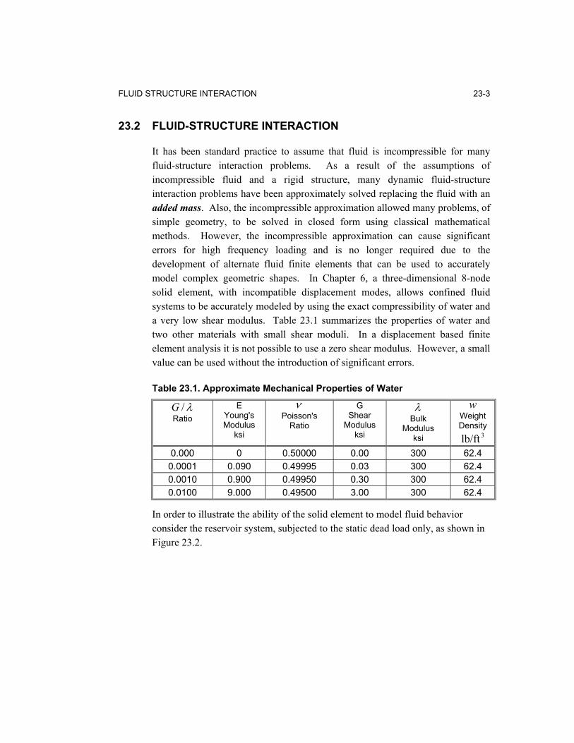
It has been standard practice to assume that fluid is incompressible for manyfluid-structure interaction problems. As a result of the assumptions ofincompressible fluid and a rigid structure, many dynamic fluid-structureinteraction problems have been approximately solved replacing the fluid with anadded mass. Also, the incompressible approximation allowed many problems, ofsimple geometry, to be solved in closed form using classical mathematicalmethods. However, the incompressible approximation can cause significanterrors for high frequency loading and is no longer required due to thedevelopment of alternate fluid finite elements that can be used to accuratelymodel complex geometric shapes. In Chapter 6, a three-dimensional 8-nodesolid element, with incompatible displacement modes, allows confined fluidsystems to be accurately modeled by using the exact compressibility of water anda very low shear modulus. Table 23.1 summarizes the properties of water andtwo other materials with small shear moduli. In a displacement based finiteelement analysis it is not possible to use a zero shear modulus. However, a smallvalue can be used without the introduction of significant errors.

Table 23.1. Approximate Mechanical Properties of Water

λ/GRatio

EYoung'sModulus

ksi

νPoisson's

Ratio

GShear

Modulusksi

λBulk

Modulusksi

wWeightDensity

3lb/ft0.000 0 0.50000 0.00 300 62.4

0.0001 0.090 0.49995 0.03 300 62.4

0.0010 0.900 0.49950 0.30 300 62.4

0.0100 9.000 0.49500 3.00 300 62.4

In order to illustrate the ability of the solid element to model fluid behaviorconsider the reservoir system, subjected to the static dead load only, as shown inFigure 23.2.


Figure 23.2. Hydrostatic Load Analysis of Reservoir Model

Note that a very thin element has been placed at the base of the reservoir in orderthat accurate fluid pressures can be calculated. For this simple example the exacthydrostatic pressure near the base of the dam is 43.33 psi and the totalhydrostatic horizontal force acting on the right vertical boundary is 312 kips perfoot of thickness. The total horizontal reactive force and the approximatestresses obtained from the finite element model, using three different materialproperties, are summarized in Table23.2.

Table 23.2. Hydrostatic Load Analysis using Fluid Finite Elements

Stresses in Fluid at Base of Dam - psiG

ShearModulus

ksi

λBulk

Modulusksi

Force Actingon RightBoundary

kips xxσ yyσ zzσ xzτ

0.0 (exact) 300 312.0 43.33 43.33 43.33 0.00

0.03 300 310.2 43.47 43.68 43.48 0.0002

0.3 300 309.6 43.41 43.40 43.48 .002

3.0 300 307.3 42.82 42.72 43.49 .025

Finite Element Model of Fluid

Shear-Free, Rigid Fluid Boundary

100 ft

100 ft100 ft

Z

X


The approximate stresses obtained using fluid elements with small shear moduliare very close to the exact hydrostatic pressure. The total horizontal force actingon the right boundary is more sensitive to the use of a small finite shear modulus.However, the error is less than one percent if the shear modulus is less or equal to0.1 percent of the bulk modulus. Therefore, this is the value of shear modulusthat is recommended for reservoir/dam interaction analysis.

In the case of a dynamic analysis of a system of fluid finite elements, the additionto the exact mass of the fluid does not introduce any additional approximations.Since the viscosity of the fluid is normally ignored in a dynamic analysis the useof a small shear modulus may produce more realistic results. Prior to anydynamic, hydrostatic loading must be applied in order to verify the accuracy andboundary conditions of the fluid-structure finite element model.

23.3 FINITE ELEMENT MODEL OF DAM-FOUNDATION INTERFACE

At the intersection of the upstream (or downstream) face of the dam with thefoundation, a stress concentration exists. A very fine mesh solution, for any loadcondition, would probably indicate very large stresses. A further refinement ofthe mesh would just produce higher stresses. However, due to the nonlinearbehavior of both the concrete and foundation material these high stresses cannotexist in the real structure. Hence, it is necessary to select a finite element modelthat predicts the overall behavior of the structure without indicating a high stressconcentration that cannot exist in the real structure.

One of the difficulties in creating a realistic finite element model is that we donot fully understand the physics of the real behavior of the dam-foundation-reservoir when the system is subjected to earthquake displacements. Forexample, if tension causes uplift at the dam-foundation interface, can shear stillbe transferred? Also, do the uplift water pressures change during loading?Because of these and other unknown factors we must use good engineeringjudgment and conduct several different finite element models using differentassumptions.

The author has had over 40 years experience in the static and dynamic finiteelement analysis of dams and many other types of structures. Based on this


experience, Figure 3 shows a typical finite element model at the interfacebetween the dam and foundation.

TWO NODES AT THESAME LOCATION

UPSTREAM FACE OF DAM

FOUNDATION

Figure 23.3. Finite Element Model of a Dam-Foundation Interface

A simple method to create a finite element model of a dam and foundation is touse eight-node solid elements for both the dam and foundation. In order toobtain the best accuracy it is preferable to use regular quadrilateral types ofmeshes whenever possible.

Note that it is always necessary to use two nodes at all interfaces between twodifferent material properties. This is because the stresses parallel to the interfaceof different materials are not equal. Therefore, two nodes at the interface arerequired in order for SAP2000 to plot accurate stress contours. The nodes mustbe located at the same point in space. However, after the two meshes for the damand foundation are created the two nodes at the interface can be constrained tohave equal displacements.

Another advantage of placing two nodes at the interface is that it may benecessary to place nonlinear gap elements at these locations in order to allowuplift in a subsequent nonlinear dynamic analysis. However, it is stronglyrecommended that a static-load, linear analysis always be conducted prior to anynonlinear analysis. This will allow the engineer to check the validity of the finiteelement model prior to a linear or nonlinear dynamic analysis.


The finite element model shown in Figure 3 indicates a layer of thin solidelements (approximately 10 cm thick) at the base of the dam since this is wherethe maximum stresses will exist. Also, in order to allow consistent foundationdisplacements it is recommended that a vertical layer of smaller elements beplaced in the foundation as shown.

Normal hydrostatic loading is often directly applied to the top of the foundationand the upstream face of the dam. If this type of surface loading is applied, largehorizontal tension stresses will exist in the foundations and vertical tensionstresses will exist at the upstream surface of the dam. In other words, the surfacehydrostatic loading tends to tear the dam from the foundation.

In the next section a more realistic approach will be suggested for the applicationof hydrostatic loads that should reduce these unrealistic stresses and produce amore accurate solution. The correct approach is to use a pore water pressureapproach that is physically realistic.

23.4 LOADING DUE TO UPLIFT AND PORE WATER PRESSURE

In the static analysis of gravity dam structures it is possible to approximate theuplift forces by a simple uplift pressure acting at the base of the dam. However,if the dam and foundation are modeled by finite elements this simpleapproximation cannot be used. The theoretically correct approach is to firstevaluate the pore water pressure at all points within the dam and foundation asshown in Figure 23.4a. The SAP2000 program has an option to perform suchcalculations.


0

10 psi

20 psi

30 psi

40 psi

50 psi

60 psi

70 psi

0

10 psi

20 psi

30 psi

40 psi60 psi

80 psi

50 psi

Porous Dam

Porous Foundation

Figure 23.4a. Water Pressure within Dam, Reservoir and Foundation

The loads associated with the pore water pressure ),,( zyxp only exist if there

are pressure gradientsdzdp

dydp

dxdp or , . Therefore, in three-dimensions the

differential forces are transferred from the water to the solid material and aregiven by

dVdzdpdf

dVdydpdf

dVdxdpdf

z

y

x

−=

−=

−=

(23.1)

Where idf is the body force in the ""i direction acting on the volume dV . The

pore water pressure loads can be treated as body forces within the standard finiteelement formulation and are consistently converted to node point loads asillustrated in Chapter. The approximate direction of these forces within the damand foundation are shown in Figure 23.4b. The SAP2000 program has the ability


to calculate pore water loading automatically and these forces can be calculatedfor both static and dynamic analysis.

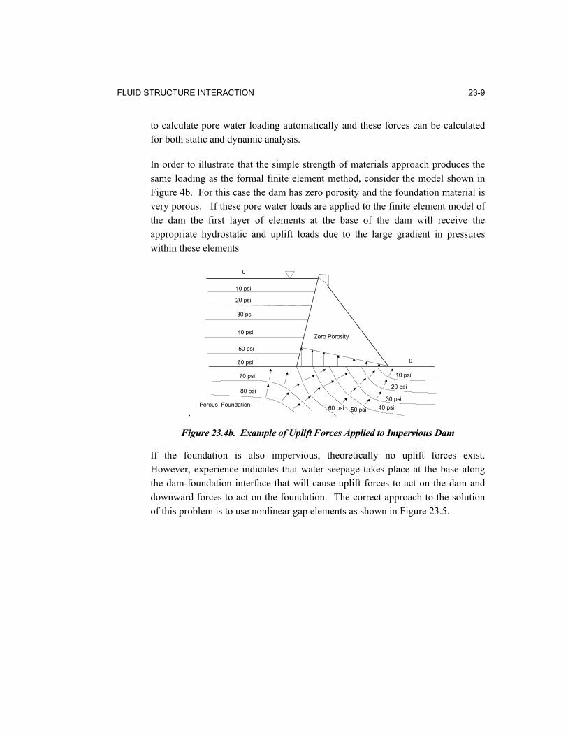
In order to illustrate that the simple strength of materials approach produces thesame loading as the formal finite element method, consider the model shown inFigure 4b. For this case the dam has zero porosity and the foundation material isvery porous. If these pore water loads are applied to the finite element model ofthe dam the first layer of elements at the base of the dam will receive theappropriate hydrostatic and uplift loads due to the large gradient in pressureswithin these elements

.

0

10 psi

20 psi

30 psi

40 psi

50 psi

60 psi

70 psi

0

10 psi

20 psi

30 psi

40 psi60 psi

80 psi

50 psi

Zero Porosity

Porous Foundation

Figure 23.4b. Example of Uplift Forces Applied to Impervious Dam

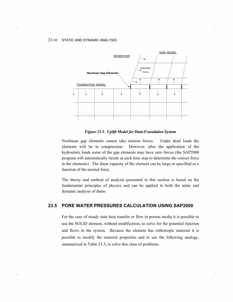
If the foundation is also impervious, theoretically no uplift forces exist.However, experience indicates that water seepage takes place at the base alongthe dam-foundation interface that will cause uplift forces to act on the dam anddownward forces to act on the foundation. The correct approach to the solutionof this problem is to use nonlinear gap elements as shown in Figure 23.5.


DAM MODEL

FOUNDATION MODEL

RESERVOIR

Nonlinear Gap Elements

Hydrostatic

Forces

Figure 23.5. Uplift Model for Dam-Foundation System

Nonlinear gap elements cannot take tension forces. Under dead loads theelements will be in compression. However, after the application of thehydrostatic loads some of the gap elements may have zero forces (the SAP2000program will automatically iterate at each time step to determine the correct forcein the elements). The shear capacity of the element can be large or specified as afunction of the normal force.

The theory and method of analysis presented in this section is based on thefundamental principles of physics and can be applied to both the static anddynamic analysis of dams.

23.5 PORE WATER PRESSURES CALCULATION USING SAP2000

For the case of steady state heat transfer or flow in porous media it is possible touse the SOLID element, without modification, to solve for the potential functionand flows in the system. Because the element has orthotropic material it ispossible to modify the material properties and to use the following analogy,summarized in Table 23.3, to solve this class of problems:


Table 23.3. Structural Analogy for the Solution of Potential Problems UsingSAP2000

I STRUCTURAL ANALYSIS ANALOGY

Let 0== yuxu and Pzu = , where P is the potential function.

The potential gradients are

xzuxP ,, = Analogous to the shear strain in the x-z plane.

yzuyP ,, = Analogous to the shear strain in the y-z plane.

zzuzP ,, = Analogous to the normal strain in the z-direction.

The potential flow equations in terms of flow properties are

xPxkxQ ,= yPykyQ ,= and zPzkzQ ,=

II COMPUTER PROGRAM INPUT

Therefore, the following material properties must be used in order tosolve steady state flow problems in three-dimensions:

xkxzG = ykyzG = and zkzE =

All other material properties are zero. The potential at a node is

specified as a displacement zu . A Concentrated node point flow into

the system is specified as a positive node force in the z direction.

Boundary points, that have zero external flows, have one unknown zu .

III COMPUTER PROGRAM OUTPUT

zu Equals the potential at the nodes.

xzτ Equals the flow in the x direction within the element.

yzτ Equals the flow in the y direction within the element.

zσ Equals the flow in the z direction within the element.

The z-reactions are node point flows at points of specified potential.


23.6 SELECTION OF GAP ELEMENT STIFFNESS VALUE

The purpose of the nonlinear gap-element is to force surfaces within thecomputational model to transfer compression forces only and not allow tensionforces to develop when the surfaces are not in contact. This can be accomplishedby connecting nodes on two surfaces, located at the same point in space, with agap element normal to the surface. The axial stiffness of the gap element must beselected large enough to transfer compression forces across the gap with aminimum of deformation within the gap element compared to the stiffness of thenodes on the surface. If the gap stiffness is too large, however, numericalproblems can develop in the solution phase.

Modern personal computers conduct all calculations using 15 significant figures.If a gap element is 1000 times stiffer than the adjacent node stiffness thenapproximately 12 significant figures are retained to obtain an accurate solution.Therefore, it is necessary to estimate the normal stiffness at the interface surfacenodes. The approximate surface node stiffness can be calculated from thefollowing simple equation:

n

s

tEAk = (23.2)

Where sA is the approximate surface area associated with the normal gapelement, E is the modulus of elasticity of the dam and nt is the finite element

dimension normal to the surface. Hence, the gap-element stiffness is given by

n

sg t

EAk 1000= (23.3)

Increasing or decreasing this value by a factor of 10 should not change the resultssignificantly.


23.7 FUNDAMENTAL EQUATIONS IN FLUID DYNAMICS

From Newton’s Second Law the dynamic equilibrium equations, in terms ofdisplacements u and fluid pressure p, for an infinitesimal fluid element are

zzyyxx upupup &&&&&& ρρρ === ,,, and , (23.4)

Where ρ is the mass density. The volume change ε of the infinitesimal fluidelement in terms of the displacements is given by the following strain-displacement equation:

zzyyxxzyx uuu ,,, ++=++= εεεε (23.5)

By definition the pressure-volume relationship for a fluid is

λε=p (23.6)

Where λ is the bulk or compressibility modulus. Elimination of the pressurefrom Equations (23.4 and 23.6) produces the following three partial differentialequations:

0)(

0)(

0 )(

,,,

,,,

,,,

=++−

=++−

=++−

zzzyzyxzzz

zyzyyyxyxy

zxzyxyxxxx

uuuuuuuuuuuu

λρ

λρ

λρ

&&

&&

&&

(23.7)

Consider the one-dimensional case 0, =− xxxx uu λρ && . For one-dimensional,

steady-state, wave propagation due to a harmonic pressure the solution is

λ

ωωω

ωωω

ωω

),(

)(),(

)(),(

)(),(

,

2

2,

2

txup

xV

tSinV

utxu

xV

tSinutxu

totxV

tSinutxu

xxx

oxxx

ox

ox

=

−−=

−−=

∞+−∞=−=

&&(23.8)


Substitution of the solution into the differential equation indicates the constantρλ /=V and is the speed at which a pressure wave propagates within the

fluid. Therefore, the speed of wave propagation is .sec/719,4 ftV = forwater. Also, the wavelength wave is given by fVL /= where f is the numberof cycles per second of the pressure loading. For several different frequencies,the maximum values of displacements and pressures are summarized in Table23.4 for a unit value of acceleration.

Table 23.4. One-Dimensional Wave Propagation in Water 0.10 =u&&

LoadingFrequency

fCycles/Sec.

Loading Frequency

fπω 2=Rad./Sec.

WaveLength

fVL /=inches

MaximumDisplacement

20 /4.386 ω=u

inches

MaximumPressure

Vu

p g

ωλ &&

= psi

2 12.57 28,260 2.4455 163.25 31.42 11,304 0.3914 62.310 62.83 5,652 0.0938 32.620 125.7 2,826 0.0245 16.330 188.5 1,884 0.0108 10.9

Note that both the maximum displacements and the pressures are reduced as thefrequency is increased for a compressible fluid.

23.8 RELATIONSHIP BETWEEN PRESSURE AND VELOCITY

One of the fundamental equations of fluid dynamics is the relationship betweenthe fluid pressure and the velocity of the fluid at any point in space. In order tophysically illustrate this relationship consider the fluid element shown in Figure6. During a small increment of time t∆ the one-dimensional wave will travel adistance tV∆ and the corresponding deformation of the element will be tu∆& .Therefore, the pressure can be expressed in terms of the velocity.


Figure 23.6. One-Dimensional Relationship Between Pressure and Velocity

The extension to three-dimensions yields

)(),,( zyx uuuVzyxp &&& ++−= ρ (23.9)

Note that the direction of a propagating wave in a fluid is defined by a velocityvector with components zyx uuu &&& and , .

23.9 EQUILIBRIUM AT THE INTERFACE OF TWO MATERIALS

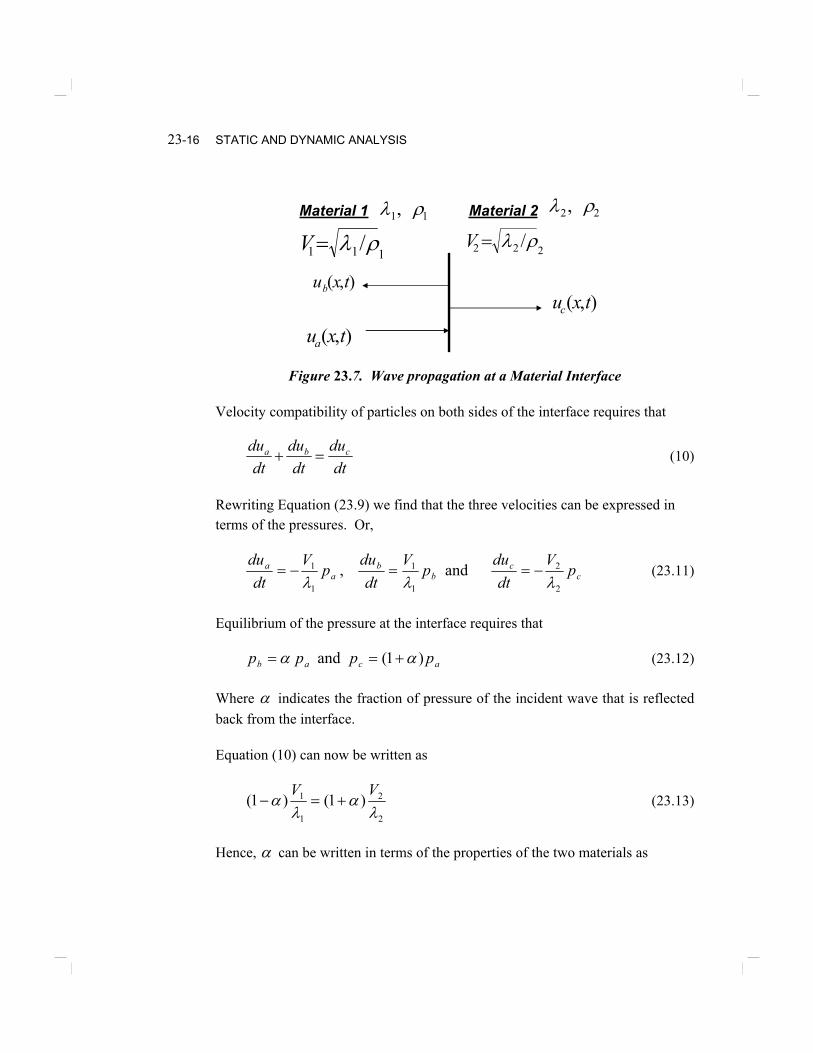
Figure (23.7) summarizes the fundamental properties that are associated with theinterface between two different materials. The bulk modulus and mass density ofthe material are ρλ and respectively.

u

tVx ∆=∆

tuu ∆+ &

Vu

xtu &&

−=∆∆

−=ε

Pressure

Volume Change

ελ=p uV

p &λ

−=

One-Dimensional Wave Propagation


Figure 23.7. Wave propagation at a Material Interface

Velocity compatibility of particles on both sides of the interface requires that

dtdu

dtdu

dtdu cba =+ (10)

Rewriting Equation (23.9) we find that the three velocities can be expressed interms of the pressures. Or,

cc

bb

aa pV

dtdupV

dtdupV

dtdu

2

2

1

1

1

1 and ,λλλ

−==−= (23.11)

Equilibrium of the pressure at the interface requires that

acab pppp )1( and αα +== (23.12)

Where α indicates the fraction of pressure of the incident wave that is reflectedback from the interface.

Equation (10) can now be written as

2

2

1

1 )1()1(λ

αλ

αVV

+=− (23.13)

Hence, α can be written in terms of the properties of the two materials as

Material 1 Material 211, ρλ 22, ρλ

222 /ρλ=V111 /ρλ=V

),( txua

),( txub),( txuc


11

22 is ratioproperty material thee wher11

ρλρλ

α =+−

= RRR

(23.14)

Therefore, the value of α varies between 1 and –1. If 1=α , the boundary isrigid and does not absorb energy and the wave is reflected 100 percent back intothe reservoir. If the materials are the same 0=α and the energy is completelydissipated and there is no reflection. If 1−=α , the boundary is very soft,compared to the bulk modulus of water, and does not absorb energy and the waveis reflected 100 percent back into the reservoir with a phase reversal.

If the value of α is known, then the material properties of material 2 can bewritten in terms of the material properties of material 1 and the known value ofα . Or,

1122 11 ρλ

ααρλ

−+

= (23.15)

23.10 RADIATION BOUNDARY CONDITIONS

From Figure 23.6. the pressure, as a function of time and space, can be writtenfor one-dimensional wave propagation as

),(),( txxuVtxp &ρλε −== (23.16)

Hence, the pressure is related to the absolute velocity by a viscous dampingconstant equal to the ρV per unit area. Therefore, linear viscous dash pots canbe inserted at the upstream nodes of the reservoir that will allow the wave to passand the strain energy in the water to “radiate” away from the dam. However,near the surface of the reservoir this is only approximate since a vertical velocitycan exist which will alter the horizontal pressure.

23.11 SURFACE SLOSHING MODES

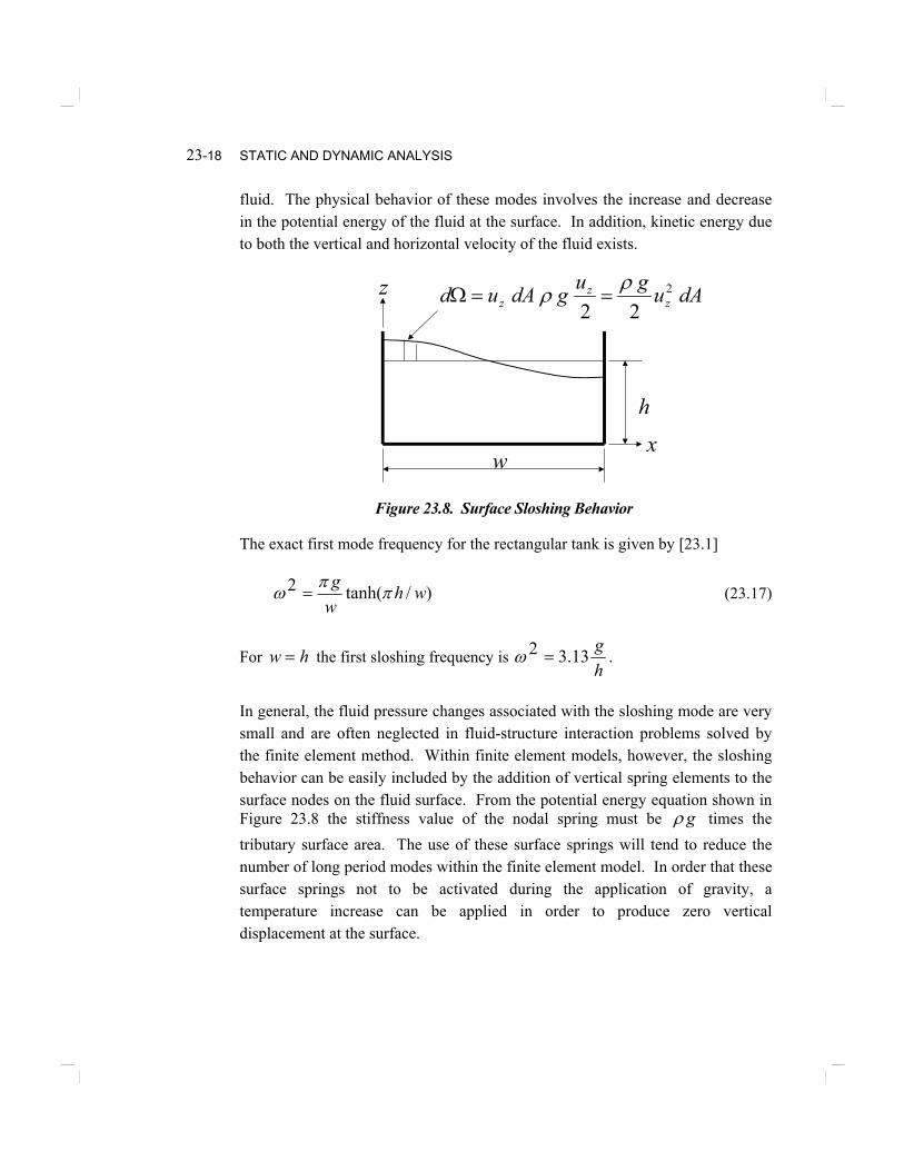
At the surface of a fluid, relatively large vertical motions are possible as shownin Figure 8. Pure sloshing motion does not involve volume change within the


fluid. The physical behavior of these modes involves the increase and decreasein the potential energy of the fluid at the surface. In addition, kinetic energy dueto both the vertical and horizontal velocity of the fluid exists.

Figure 23.8. Surface Sloshing Behavior

The exact first mode frequency for the rectangular tank is given by [23.1]

)/tanh(2 whwg

ππ

ω = (23.17)

For hw = the first sloshing frequency is hg13.32 =ω .

In general, the fluid pressure changes associated with the sloshing mode are verysmall and are often neglected in fluid-structure interaction problems solved bythe finite element method. Within finite element models, however, the sloshingbehavior can be easily included by the addition of vertical spring elements to thesurface nodes on the fluid surface. From the potential energy equation shown inFigure 23.8 the stiffness value of the nodal spring must be gρ times thetributary surface area. The use of these surface springs will tend to reduce thenumber of long period modes within the finite element model. In order that thesesurface springs not to be activated during the application of gravity, atemperature increase can be applied in order to produce zero verticaldisplacement at the surface.

x

z

h

w

dAugugdAud zz

z2

22ρρ ==Ω


23.12 VERTICAL WAVE PROPAGATION

Due to the existence of the free surface of the reservoir water can move verticallydue to horizontal boundary displacements. These vertical waves are coupledwith the horizontal displacements, since the water pressure is equal in alldirections. If no horizontal motion exists, resonant vertical waves can still existwith a displacement given by the following equation:

3,2,1for )()2

12(),( =−

= ntSinzh

nSinUtzu nnz ωπ .. (23.18)

Note that the vertical shape function satisfies the boundary conditions of zerodisplacement at the bottom and zero pressure at the surface of the reservoir.Substitution of Equation 18 into the vertical wave equation, zzzuzu , λρ =&& ,

produces the following vertical frequencies of vibration:

hVnfzV

hn

nn 412 Or,

212 −

=−

= πω (23.19)

Therefore, for a reservoir depth of 100 feet the first frequency is 11.8 cps and thesecond frequency is 34.4 cps. For a reservoir depth of 200 feet the first twofrequencies are 5.9 and 17.2 cps. Also, these vertical waves do not haveradiation damping (if the bottom of the reservoir is rigid) as in the case of thehorizontal waves propagating from the upstream face of the dam. The excitationof these vertical modes by horizontal earthquake motions is very significant formany dam-reservoir systems. However, silt at the bottom of the reservoir cancause energy absorption and reduce the pressures produced by these verticalvibration modes.


23.13 THE WESTERGAARD PAPER

Approximately seventy years ago Westergaard published the classical paper on“Water Pressure on Dams during Earthquakes” [23.2]. His paper clearlyexplained the physical behavior of the dam-reservoir interaction problem. Thepurpose of his work was to evaluate the pressure on Hoover dam due toearthquake displacements at the base of the dam.

Westergaard’s work was based on the solution of the simple two-dimensionalreservoir/dam system, shown in Figure 9, subjected to horizontal earthquakedisplacement motion of )()( 0 tSinutu xx ω= at the base of the dam.

)sin(),(2

tu

ztu gdamx ω

ω&&

−=

z

x

∞=≈ xztu waterx at 0),(

∞=−= to0 at x )sin()(2 t

utu g

foundationx ωω&&

0)( =tuz

h

x

b(z)

Figure 23.9. Rigid Dam and Reservoir Model

Since simple harmonic motion is assumed, the displacement is related to theacceleration by the following equation:

20

0 Or, )(02)(

ωωω xu

xutSinxutxu&&

&& −=−= (23.20)

Westergaard solved the two dimensional compressible wave equations(Equations 7) by separation of variables. For a rectangular reservoir the solutionis an infinite series of space and time functions. He then concluded (based on a1.35 second measured period during the great earthquake in Japan in 1923) thatthe period of earthquake motions (displacements) could be assumed to be


greater than a second. Therefore, he assumed and earthquake period of 1.333seconds, the exact compressibility of water and approximated the exact pressuredistribution with a parabolic distribution. Based on these assumptions,Westergaard presented a conservative approximate equation for a the pressuredistribution for a rigid dam as

guzbguzhhzp &&&& ρρ )()(87)( =−= (23.21)

where ρ is the mass density of water; or gw /=ρ . The term )(zb can bephysically interpreted as the equivalent amount of water that will produce thesame pressure for a unit value of horizontal acceleration gu&& of a rigid dam. The

term added mass was never used or defined by Westergaard.

Theodor von Karman, in a very complimentary discussion of the paper, used theterm apparent mass. Based on an incompressible water model and an ellipticalpressure approximation he proposed the following equation for the pressure atthe reservoir-dam vertical interface as

guzbguzhhzp &&&& ρρ )()(707.0)( =−= (23.22)

One notes that the difference between the two approximate equations is not ofgreat significance. Therefore, the assumption of 1.333 seconds earthquakeperiod by Westergaard produces almost the same results as the von Karmansolution.

Unfortunately, the term ρ)(zb has been termed the added mass by others andhas been misused in many applications with flexible structures using the relativedisplacement formulation for earthquake loading. All of Westergaard’s workwas based on the application of the absolute displacement of the earthquake atthe base of the dam. For non-vertical upstream dam surfaces, some engineershave used this non-vertical surface pressure, caused by the horizontal earthquakemotions, as an added mass in the vertical direction. The use of this vertical massin an analysis due to vertical earthquake loading has no theoretical basis.


According to Westergaard, due to the high pressures at the base of the reservoirthe water tends to escape to the surface of the reservoir. In addition, we will findin many reservoirs that the vertical natural frequencies are near the horizontalfrequencies of the dam and the frequencies contained in the earthquakeacceleration records.

23.14 DYNAMIC ANALYSIS OF RECTANGULAR RESERVOIR

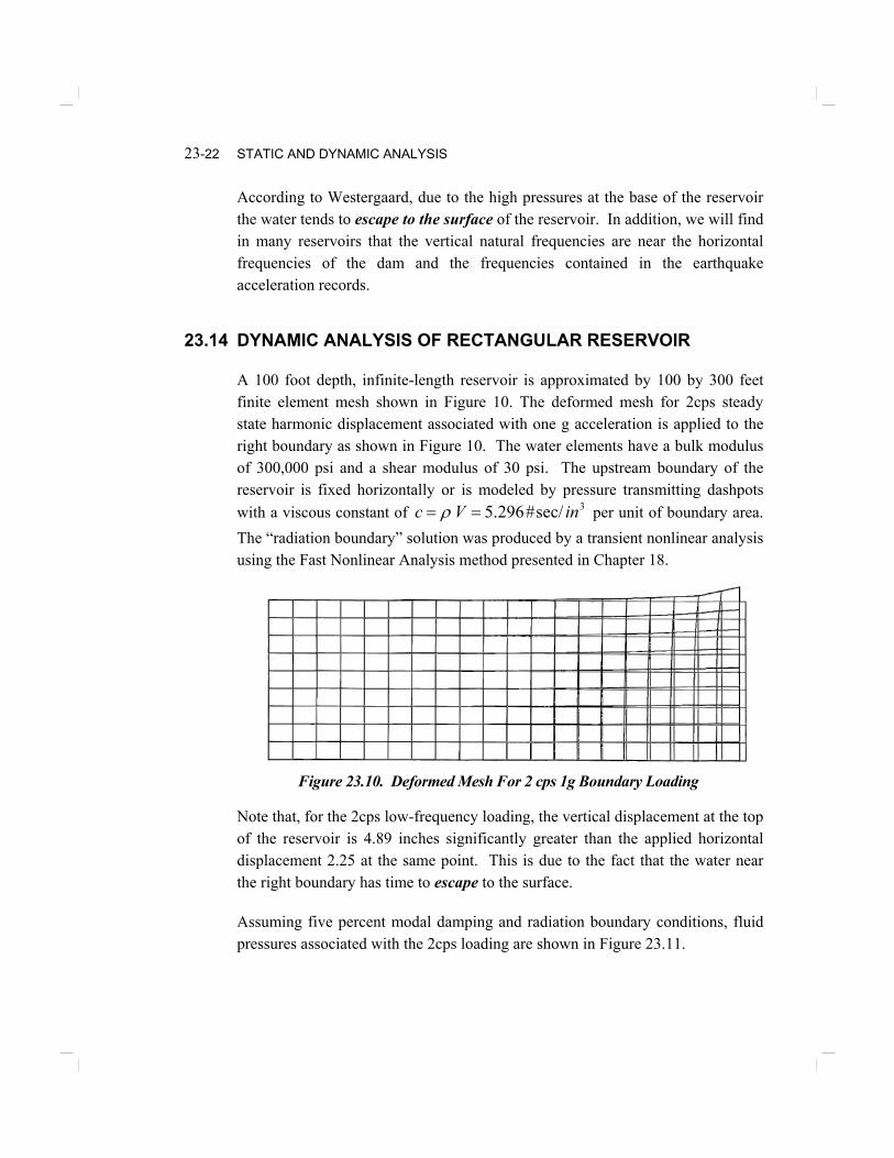
A 100 foot depth, infinite-length reservoir is approximated by 100 by 300 feetfinite element mesh shown in Figure 10. The deformed mesh for 2cps steadystate harmonic displacement associated with one g acceleration is applied to theright boundary as shown in Figure 10. The water elements have a bulk modulusof 300,000 psi and a shear modulus of 30 psi. The upstream boundary of thereservoir is fixed horizontally or is modeled by pressure transmitting dashpotswith a viscous constant of 3sec/#296.5 inVc == ρ per unit of boundary area.The “radiation boundary” solution was produced by a transient nonlinear analysisusing the Fast Nonlinear Analysis method presented in Chapter 18.

Figure 23.10. Deformed Mesh For 2 cps 1g Boundary Loading

Note that, for the 2cps low-frequency loading, the vertical displacement at the topof the reservoir is 4.89 inches significantly greater than the applied horizontaldisplacement 2.25 at the same point. This is due to the fact that the water nearthe right boundary has time to escape to the surface.

Assuming five percent modal damping and radiation boundary conditions, fluidpressures associated with the 2cps loading are shown in Figure 23.11.


Figure 23.11. Pressure Distribution Times 10 for 2 cps 1g Boundary Loading

The maximum finite element pressure of 36.3 psi compares very closely with theadded mass solution of 37.9 psi from Eq. (23.21). Because the finite elementmodel has mass lumped at the surface, the zero pressure condition is notidentically satisfied. A finer mesh near the surface would reduce this error.

The pressure distribution associated with 30 cps one g loading at the rightboundary is shown in Figure 12. and illustrates the wave propagation associatedwith the 30 cps frequency loading. The apparent quarter wave length isapproximately 120 feet. The exact one-dimensional, quarter-wave lengthassociated with 30 cps in water is 33.25 feet. The difference is due to free-surface of the reservoir which allows vertical movement of the water. Of coursethe wave length associated with the incompressible solution is infinity.

Figure 23.12. Pressure Distribution Times 10 for 30 cps 1g Boundary Loading


Table 23.4 summarizes the maximum pressure obtained using different boundaryconditions at the upstream face of the reservoir and different values for modaldamping. Since the loading is simple harmonic motion many differentfrequencies of the reservoir tend to be excited by all loadings. The first verticalfrequency is 11.9 cps and the second vertical frequencies 34.4 cps. Thesepartially damped resonant frequencies should not be excited to the same degreeby typical earthquake type of loading which contain a large number of differentfrequencies.

Table 23.4. Water Pressure vs. Frequency of Loading for a 300 ft. by 100 ft Reservoir

Added Mass Pressure Equals 37.9 psi for all Frequencies

From this simp

Due to a singularity in the Westergaard solution the results are not valid forloading frequencies above 10 cps. However, from this simple study it is apparentthat for low frequency loading, under 5 cps, the added mass solution is anacceptable approximation. However, for high frequencies, above 5 cps, theincompressible solution is not acceptable. For 30 cps the finite element pressureof 11.5 psi, is shown in Figure 12. At the bottom of the reservoir the finiteelement solution approaches the exact, wave-propagation solution of 10.9 psi fora confined one-dimensional problem. Normally, one would not expect that an

Finite Element Fluid

Model Maximum

Pressures psi

Loading

Frequency

CPS

Modal

Damping

Percent Fixed

Upstream

Boundary

Radiation

Upstream

Boundary

Westergaard

Compressible

Solution

No Damping

psi

Confined

One D.

Wave

Propagation

No Damping

psi

2 0.1 56.6 29.6 35.9 163.2

2 1.0 28.6 28.3 35.9 163.2

2 5.0 40.4 36.3 35.9 163.2

5 5.0 34.8 33.5 39.1 65.2

10 5.0 60.7 53.4 66.9 32.6

20 5.0 56.6 58.3 na 16.3

30 5.0 14.9 11.5 na 10.9


increase in damping, for the same loading, would cause an increase in pressure.However, this is possible as illustrated in Chapter 22.

23.15 ENERGY ABSORPTIVE RESERVOIR BOUNDARIES

In addition to the ability of the fluid finite element to realistically capture thedynamic behavior of rectangular reservoirs, it has the ability to model reservoirsof arbitrary geometry and the silt layer at the bottom of the reservoir. Table 23.6summarizes measured reflection coefficients for bottom sediments and rock atseven concrete dams [23.4].

Table 23.6. Measured Reflection Coefficients for Several Dams

Dam Name Bottom Material αFolsom Bottom Sediments With Trapped Gas, Such

As From Decomposed Organic Matter-0.55

Pine Flat Bottom Sediments With Trapped Gas, SuchAs From Decomposed Organic Matter

-0.45

Hoover Bottom Sediments With Trapped Gas, SuchAs From Decomposed Organic Matter

-0.05

Glen Canyon Sediments 0.15

Monticello Sediments 0.44

Glen Canyon Rock – Jurassic Navajo Sandstone 0.49

Crystal Rock – Precambrian Metamorphic Rock 0.53

Morrow Point Rock – Biotite, Schist Mica Schist,Micaceous Quartzite, And Quartzite

0.55

Monticello Sandstone Interbedded With Sandy ShaleAnd Pebbly Conglomerate

0.66

Hoover Rock Canyon Walls 0.77

It is apparent that the reflection coefficient is a function of the thickness andproperties of the bottom sediment and the properties of the underlying rock at aspecific location within the reservoir.

The reflection coefficient α is the ratio of the “reflected” to “incident” waveamplitudes. The value of α varies between 1 and –1. If 1=α , the boundary isrigid and does not absorb energy and the wave is reflected 100 percent back into


the reservoir. If 0=α , the energy is completely dissipated and there is noreflection. If 1−=α , the boundary is very soft, compared to the bulk modulusof water, and does not absorb energy and the wave is reflected 100 percent backinto the reservoir with a phase reversal.

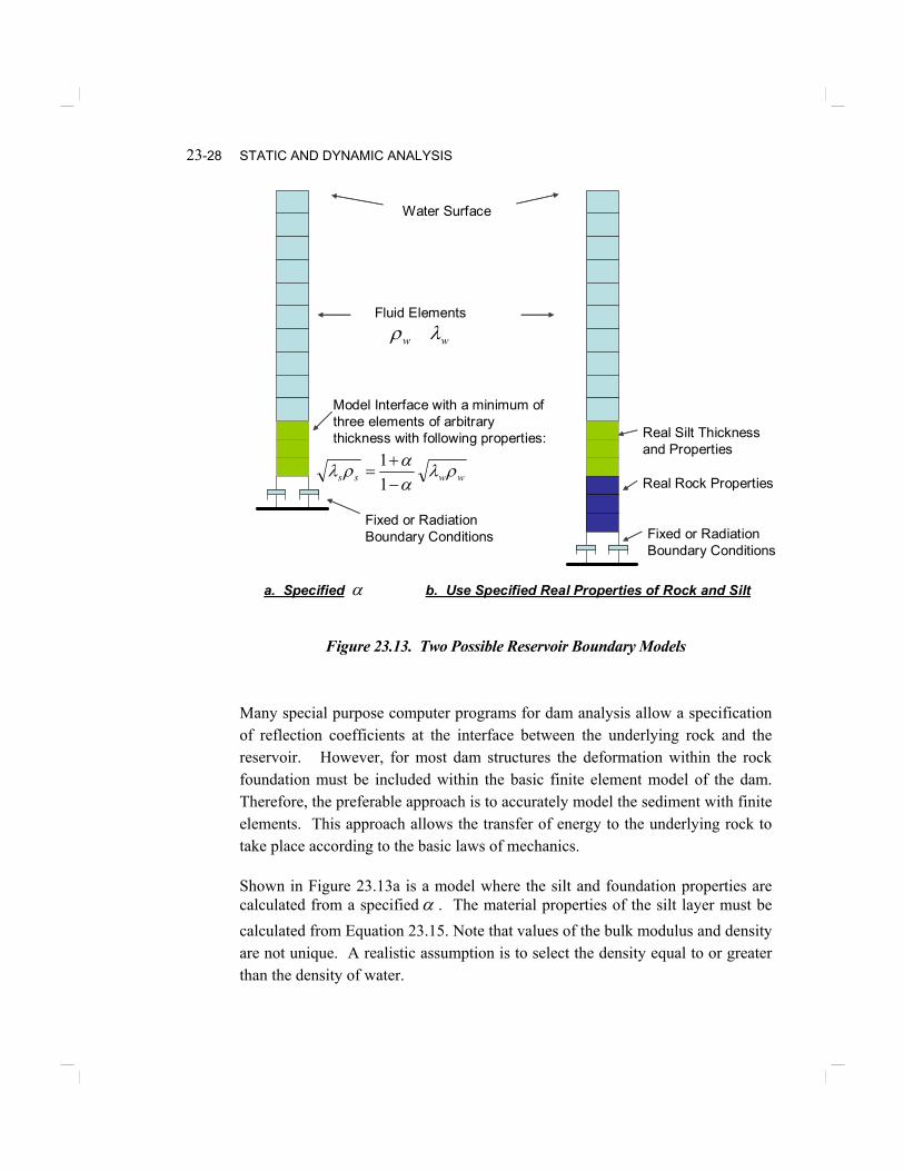
Figure 23.13 illustrated two possible finite element models to simulate thedynamic behavior at the interface between the reservoir and boundary.


Fluid Elements

ww λρ

Model Interface with a minimum of three elements of arbitrary thickness with following properties:

wwss ρλααρλ

−+

=11

a. Specified α b. Use Specified Real Properties of Rock and Silt

Fixed or Radiation Boundary Conditions Fixed or Radiation

Boundary Conditions

Real Silt Thickness and Properties

Real Rock Properties

Water Surface

Figure 23.13. Two Possible Reservoir Boundary Models

Many special purpose computer programs for dam analysis allow a specificationof reflection coefficients at the interface between the underlying rock and thereservoir. However, for most dam structures the deformation within the rockfoundation must be included within the basic finite element model of the dam.Therefore, the preferable approach is to accurately model the sediment with finiteelements. This approach allows the transfer of energy to the underlying rock totake place according to the basic laws of mechanics.

Shown in Figure 23.13a is a model where the silt and foundation properties arecalculated from a specified α . The material properties of the silt layer must becalculated from Equation 23.15. Note that values of the bulk modulus and densityare not unique. A realistic assumption is to select the density equal to or greaterthan the density of water.


A more general finite element model for the base and walls of the reservoir isshown in Figure 13b. If a significant amount of the rock foundation is modeled,using large elements, it may not be necessary to use radiation boundaryconditions as illustrated in Chapter 16.

23.16 RELATIVE VERSUS ABSOLUTE FORMULATION

A two-dimensional view of a typical dam-foundation-reservoir-gate system,subjected to absolute earthquake displacements, was shown in Figure 1.However, if foundation-dam interaction is to be considered it is necessary toformulate the analysis in terms of the displacements relative to the free fielddisplacements that would be generated without the existence of the dam andreservoir. Figure 23.6 illustrates the type of loading that is required if a relativedisplacement formulation is used.

Reservoir

Dam

Foundation

Gate

dxg mtu )(&&

dzg mtu )(&&wzg mtu )(&&

wxg mtu )(&&

)(tuxg Applied Ground Displacements

No Forces Applied to Foundation

Fixed or Radiation Boundary Conditions

Figure 23.14. Relative Displacement Formulation of Dam-Reservoir System

It can easily be shown, for the relative displacement formulation, that the loadingon the reservoir, dam and gate is the mass times the ground acceleration. In


order to simulate the upstream reservoir boundary condition it is necessary toapply the negative horizontal ground displacements to the upstream face of thereservoir in addition to inertial loading on the water elements. If the foundationof the system is included, no inertial load is applied to the foundation elements.However, the mass of the foundation must be included in the evaluation of theshape functions to be used in the mode superposition dynamic analysis of thecomplete system

23.17 THE EFFECT OF GATE SETBACK ON PRESSURE

Radial gates are normally set back from the upstream face of the dam as shownin Figure 23.15. One question that requires an answer is: does the setbackincrease or decrease the pressure acting on the gate? Also, how does onecreate a finite element model of the reservoir in order to avoid the displacementsingularity at the intersection of the upstream face of the dam and theapproximately horizontal spillway?


100’

30’

10’300’

Singularity: ?0 == xz uu

Figure 23.15. Reservoir With Radial Gate Setback

The second question must be addressed first in order to evaluate the effects of thesetback on the pressure distribution. Due to the applied displacements at theright boundary, there should be a relatively large vertical displacement at thisintersection; however, due to the existence of the horizontal surface the verticalwater displacement should be zero. In addition, the horizontal displacement ofthe water must be equal to the applied displacement; however, the horizontalmovement of the water on top of the spillway must be allowed to movehorizontally if the correct pressures are to be developed at the base of the gate.One can approximate this behavior by reducing the stiffness of the water elementnear this singularity. A preferable approach is to create additional nodes at thesingular point and to allow the discontinuity in displacements to exist. A finiteelement mesh, that satisfies these requirements, is shown in Figure 23.16.


DAM

)()( damuwateru zz =

)()( damuwateru xx =

)()(

loweruupperu

z

z =

)()( rightuleftu xx =

Figure 23.16. Suggested Mesh at Intersection of Upstream and Spillway Surfaces

Inserting shear-free horizontal and vertical interfaces between the dam andreservoir and between different areas of the reservoir allows all boundaryconditions to be satisfied. Note that it is not necessary to add additionalelements. However, the vertical displacements will not be equal on the two sidesof the vertical interface and the horizontal displacement will not be equal at thetop and bottom of the horizontal interface. Near the surface several of the fluidnodes on the vertical fluid may be constrained to have the same vertical andhorizontal displacements in order that the surface displacements are continuous.

The finite element mesh used to study the setback problem is shown in Figure23.17. The maximum pressures due to a 2 cps 1 g boundary loading with zerodamping and no radiation damping, are summarized in Table 23.6 for the casesof with and without gate setback.


Table 23.6. Summary of Pressures With and Without Gate Setback

With Gate Setback Without Gate Setback

Pressure at Base of Gate 16.5 psi 20.6 psi

Pressure at Base of Dam 31.9 psi 33.6 psi

From this simple example it is apparent that the setback of the gate from theupstream face of the dam reduces the pressures acting on the gate and at the baseof the dam. Since the setback increases the surface area of the reservoir, thewater below the base of the gate can escape to the surface more easily; therefore,all pressures are reduced.

Figure 23.17. Finite Element Mesh for Reservoir with Gate Setback


23.18 SEISMIC ANALYSIS OF RADIAL GATES

A significant number of seismic analyses of radial gates have been conductedbased on a two stage dynamic analysis. First the dam, without the gate, isanalyzed for the specified ground motions. In most cases the added massapproach is used to approximate the dynamic behavior of the dam and reservoir.The acceleration obtained from this analysis, at the location of the gate, is thenapplied to a separate finite element model of the gate only. The reservoirassociated with gate is approximated by an added mass calculated using the totaldepth of the reservoir. The model of the gate, with the reservoir added mass, isthen subjected to the accelerations history (or the corresponding responsespectra) calculated from the dam analysis model.

In many cases the two dynamic analyses are conducted using different computerprograms. This is because many special purpose dam analysis programs do notcontain three dimensional frame and shell elements that are required toaccurately model the steel gates. In addition, the two stage dynamic analysis isbased on incompressible fluid and rigid structure assumptions.

During the past three years the author has conducted several seismic analyses ofseveral dam-reservoir-gate systems using one model where the reservoir has beenmodeled by compressible fluid elements and the gate accurately modeled bybeam and shell elements [3]. In addition to the improved accuracy of thisapproach there is significant reduction in the amount of manpower in thepreparation of only one model. Also, there is no need to calculate added massand it is not necessary to transfer the output from one dynamic analysis as theinput data for a separate gate model. Therefore, the one three-dimensionaldynamic analysis is simpler than the commonly used two stage approach. Thecomputer time requirements for the dynamic analysis of this comprehensivemodel are approximately one hour using an inexpensive personal computer.However, the preparation and verification of a large finite element model stillrequires a significant amount of engineering time. Therefore, there is amotivation to use a more simplified model to evaluate the seismic safety of radialgates. The following is a list on modeling assumptions that may help to reducethe amount of manpower required to prepare the finite element model:


1. We have found that a fine mesh, shell-element model of the gate and supportbeams is necessary in order to capture the complex interaction of the face ofthe gate with the backup beam structure. This level of detail is necessary tomatch the measured frequencies of the dry gate, and to produce realisticstresses in the gate structure. The arms and diagonal braces of the gate canbe modeled with frame elements that neglect secondary bending stresseswithin the one-dimensional elements.

2. We found that both the dry and wet frequencies of a typical gate are high anddo not significantly affect the total dynamic loads on the gate and trunnion.For the gate studied in reference [3], it was found that if the modulus ofelasticity of the steel of the gate was doubled, the maximum earthquakereaction at the trunnion was increased by less than 10 percent. Therefore, itmay be possible to use a coarse finite element mesh to model the face of thegate, along with a three-dimensional model of the reservoir and dam, toobtain the maximum dynamic pressure acting on the gate.

3. A second option for simplifying the modeling is based on the fact that thedynamic pressure distribution was found to be approximately the same at thecenter and at the edges of the gate, indicates that a coarse mesh, along theaxis of the gate, can be used to model the reservoir upstream of the gate. Itappears that excellent results can be produced if fewer layers of reservoirelements are used along the horizontal axis of the gate.

4. Formal constraint equations can be used to connect the fine mesh gate to thecoarse mesh reservoir. However, the steel gate is very stiff compared to thestiffness of water; therefore, the fine mesh steel elements will automaticallybe compatible with the coarse mesh water elements and formal constraintequations are not required.

5. This approach of using a coarse mesh reservoir and fine mesh gate model inthe same analysis appears to be more accurate and will require lessengineering time than the approximate two stage analysis suggested in theprevious paragraph. Physically, this approximation is similar to lumping thewater mass at the coarse mesh nodes between the gate and reservoir.Therefore, these nodes should be located at nodes on the face of the gate


where the ribs and beams exist. This approximation neglects bendingstresses in the face plate between the ribs. However, one can approximatelycalculate these additional bending stresses from simple beam equations. Or,one can ignore these bending stresses since local yielding in the face plateswill not cause the failure of the gate.

6. For a straight gravity dam the same number of layers used to model thereservoir should be used to model the dam and foundation. This planemodel, coupled with a fine-mesh, three-dimensional, shell/beam model of thegate, should produce acceptable results. It is important that the maximumdepth of the reservoir below the gate is used for the plane model. A three-dimensional model of the dam and reservoir, including the V-shape of thecanyon, will produce lower pressures on the gate. Therefore, this “planarslice” should be conservative. Vertical earthquake motions applied to thismodel should produce conservative water pressures, since the water isconstrained from lateral movement in this formulation

7. For an arch or curved dam a three-dimensional, coarse mesh model of thedam, foundation and reservoir should be created in order to accuratelycapture the complex dynamic interaction between the reservoir, dam andfoundation. The coarse mesh model can be coupled with a fine mesh modelof a typical gate. The combined system can be subjected to all threecomponents of earthquake displacements and the resulting analysis should berealistic since a minimum number of approximations have been introduced.

8. After a careful study of the dynamic behavior of the water above thespillway, between the upstream face of the gate and the upstream face of thedam, it appears that this volume of water can be eliminated from thereservoir model. This can be accomplished by moving the fine mesh modelof the gate and trunnion upstream so that the base of the face of the gate is atthe same location as the upstream face of the dam. This assumption willsimplify the model and allow the water to move freely in the verticaldirection during dynamic loading and transfer reservoir pressure fluctuationsdirectly to the gate structure. Parameter studies have indicated that thisapproximation produces slightly conservative results. Stiff link elements,


normal to the upstream face of the dam and radial gate, must be used toconnect the reservoir and structure.

9. A horizontal boundary, with two nodes at the same location, should belocated at the elevation of the contact between the gate and spillway andextend to the upstream boundary of the reservoir. These nodes should haveequal vertical displacements and independent horizontal displacements. Thiswill allow the bottom of the gate to move relative to the top of the spillway.The same type of boundary should exist between the foundation and thereservoir.

23.19 FINAL REMARKS

The classical approximation of incompressibility was first introduced to simplifythe mathematics in order to obtain a closed form mathematical solutions of fluiddynamics problems with simple geometry. In addition, added massapproximation is valid only for low frequencies under 5 cps. However, theseapproximations are not required at the present time due to the development ofthree-dimensional fluid elements, inexpensive, high-speed computers and otherefficient numerical method of dynamic analysis. Also, dam/reservoir/gate/foundation systems of arbitrary geometry can all be included in the samemodel.

Viscous forces within the fluid and the frictional forces between the dam-foundation-gate and the reservoir have been neglected. Therefore, theassumption of five percent damping appears to be a reasonable approximationuntil further research is conducted. It may be worthwhile to conduct an analysisof a two dimensional, computational fluid dynamic analysis of a reservoir only,where the real viscosity of the water is included in order to verify that equivalentmodal damping can be used to approximate the viscous energy dissipation.Additional experimental research and parameter studies for one and twodimensional finite element models must be conducted to evaluate the sensitivityof all damping assumptions.

The upstream reservoir mesh should be approximately four times the maximumdepth of the reservoir. If foundation deformations are significant, the foundation


mesh should extend downstream and below the dam a distance equal to twotimes the upstream/downstream width of the base of the dam. Inertia loadsshould not be applied to the foundation elements. However, the foundation massmust be included in the calculation of the mode shapes.

The mesh should be coarse at the base and near the upstream vertical boundary ofthe reservoir. The finest mesh, in both the horizontal and vertical directions,should be near the upstream face or the dam or gate.

The finite element fluid model and boundary conditions must be verified by theapplication of vertical dead load to the reservoir. The total horizontal hydrostaticforce applied to the face of the dam and gate can be calculated from staticequilibrium equations and should be within few percent of the finite elementsolution. In addition, the stresses (pressure) within the water elements

zyx σσσ and, should be approximately equal. Also, the hydrostatic pressure

at the base of the reservoir, obtained from the finite elements model, should bevery close to the weight of a unit area of water above the node.

After the static model is verified by the plotting of stresses and deflected shapes,the natural eigenvectors, including both static and dynamic modes, should becalculated and plotted. Both the total static and mass participation factors shouldbe examined. One hundred percent static participation is required and overninety percent of the mass participation in all the directions of earthquake loadingis required to assure a converged solution.

23.20 REFERENCES

1. Cook, R., D. Malkus and M. Plesha, “Concepts and Applications of FiniteElement Analysis”, Third Edition, John Wiley and Sons, Inc., 1989.

2. Westergaard, H. M. “Water Pressure on Dams During Earthquakes”,Transactions, ASCE, Vol. 9833, Proceedings November 1931.

3. Aslam M., Wilson E.L., Button M. and Ahlgren E., "Earthquake Analysis ofRadial Gates/Dam Including Fluid-Structure Interaction," Proceedings, Third


U.S.-Japan Workshop on Advanced Research on Earthquake Engineering forDams, San Diego, CA. June 2002.

4. Engineering Guidelines for the Evaluation of Hydropower Projects, FederalEnergy Regulatory Commission.

draft dated: monday, august 25, 2003 contents of chapter 23edwilson.org/book/23-fluid.pdf ·...

Documents