
Volker Britz, Jean-Jacques Herings, Arkadi Predtetchinski Theory of the Firm: Bargaining and Competitive Equilibrium RM/10/057

Theory of the Firm: Bargaining and Competitive
Equilibrium1
Volker Britz2 P. Jean-Jacques Herings3 Arkadi Predtetchinski4
November 15, 2010
1The authors would like to thank Jacques Dreze for helpful comments and suggestions.2V. Britz ([email protected]), Department of Economics, Maastricht University.
This author would like to thank the Netherlands Organisation for Scientific Research (NWO) forfinancial support.
3P.J.J. Herings ([email protected]). Department of Economics, MaastrichtUniversity. This author would like to thank the Netherlands Organisation for Scientific Research(NWO) for financial support.
4A. Predtetchinski ([email protected]), Department of Economics,Maastricht University. This author would like to thank the Netherlands Organisation for ScientificResearch (NWO) for financial support.

Abstract
Suppose that a firm has several owners and that the future is uncertain in the sense
that one out of many different states of nature will realize tomorrow. An owner’s time
preference and risk attitude will determine the importance he places on payoffs in the
different states. It is a well–known problem in the literature that under incomplete asset
markets, a conflict about the firm’s objective function tends to arise among its owners. In
this paper, we take a new approach to this problem, which is based on non–cooperative
bargaining. The owners of the firm play a bargaining game in order to choose the firm’s
production plan and a scheme of transfers which are payable before the uncertainty about
the future state of nature is resolved. We analyze the resulting firm decision in the limit of
subgame–perfect equilibria in stationary strategies. Given the distribution of bargaining
power, we obtain a unique prediction for a production plan and a transfer scheme. When
markets are complete, the production plan chosen corresponds to the profit-maximizing
production plan as in the Arrow-Debreu model. Contrary to that model, owners typically
do use transfers to redistribute profits. When markets are incomplete, the production plan
chosen is almost always different from the standard notion of competitive equilibrium and
again owners use transfers to redistribute profits. Nevertheless, our results do support the
Dreze criterion as the appropriate objective function of the firm.
Keywords: Strategic bargaining, Nash bargaining solution, incomplete markets, stock
market equilibrium, objective function of the firm, profit-maximization.
JEL codes: C78, D52.

1 Introduction
Suppose that a firm has several owners and that the future is uncertain in the sense that
one out of many different states of nature will realize tomorrow. An owner’s time preference
and risk attitude will determine the importance he places on payoffs in the different states.
It is a well–known problem in the literature that under incomplete asset markets, a conflict
about the firm’s objective function tends to arise among its owners.
We take a non-cooperative bargaining approach to this conflict, which is new to the
literature. We present a model in which the internal decision making of the firm is for-
malized explicitly as a strategic bargaining game. In contrast to standard theory, we thus
consider the firm as a coalition of owners who use strategic power in order to influence the
firm’s production decision and thereby maximize their own payoffs.
The standard approach in the existing literature on incomplete markets with produc-
tion originates from contributions by Diamond (1967), Dreze (1974), and Grossman and
Hart (1979). Diamond (1967) formulates the notion of constrained Pareto optimality,
an optimality notion that takes the incompleteness of asset markets into account. Dreze
(1974) shows that necessary first-order conditions for constrained Pareto optimality require
that the firm should choose a production plan which is optimal when evaluated against a
weighted average of the shareholders’ utility gradients, where the weights are given by the
ownership shares. This objective function for the firm is usually referred to as the Dreze
criterion.
Standard notions of constrained Pareto optimality allow for arbitrary redistributions
in the initial period, and so does Dreze (1974), pp. 141–142:
“The definition does not place any restrictions on the allocation among con-
sumers of the adjustments in current consumption required to offset the adjust-
ment in the input level aj− aj. Alternatively stated, the definition is consistent
with arbitrary transfers of initial resources among consumers.”
Arbitrary redistributions in the initial period leads to indeterminateness of equilibrium.
With H shareholders, one would in general expect a multiplicity of degree H − 1.
Grossman and Hart (1979) use the Dreze criterion as the objective function for the firm,
but with final ownership shares replaced by initial ones. Contrary to Dreze (1974), they also
require that at equilibrium no transfers are made in the initial period. The advantage of this
approach is that it leads to determinateness of equilibrium, its downside is inconsistency.
Indeed, initial period transfers are used in Grossman and Hart (1979) in their definition
of constrained Pareto optimality, which motivates the decision criterion for the firm. At
1

the same time, the equilibrium decision of the firm is imposed to involve no transfers
itself. Absence of initial-period transfers has become the standard concept of equilibrium,
called stock market equilibrium, see for instance the treatment in the authoritative book
of Magill and Quinzii (1996) and in the paper by Dierker, Dierker, and Grodal (2002) on
the constrained inefficiency of stock market equilibria.
Recognizing that the Dreze criterion is normative in nature, some authors have tried
to link it to outcomes of majority voting. A typical approach in this stream of literature
is to ask: If a certain production plan was given as a default option, would there exist an
alternative plan preferred by more than at least a certain (super-)majority of the sharehold-
ers? If no winning alternative can be found, the default plan is considered “stable.” Tvede
and Cres (2005) discuss the relationship between the Dreze criterion and such a voting
approach and find conditions under which both lead to compatible predictions. Another
voting analysis is given by DeMarzo (1993) who emphasizes the importance of the largest
shareholder. Kelsey and Milne (1996) give a proof for equilibrium existence in a more gen-
eral model which emphasizes externalities between firms and shareholders. However, both
stock market equilibria and the approaches related to majority voting seem to suffer from
a common problem. Both approaches ask only which production plans are stable to being
replaced by other plans through a certain mechanism. However, there is no explanation
why a particular plan would serve as a default setting or how any one particular plan is to
be chosen in case there are several plans satisfying the criterion used.
Few papers have taken a truly positive approach to decision making within the firm,
as is the case in this paper.
In our setup, there is a single firm which exists in an environment of competitive but
potentially incomplete markets. We take the ownership structure of the firm as exogenously
fixed to focus attention on the decision making within the firm, rather than on the role of
expectations regarding future stock price as a consequence of current production decisions
and the identity of future shareholders as in Bonnisseau and Lachiri (2004) and Dreze,
Lachiri, and Minelli (2009). When applied to our setting without stock markets, we refer
to the stock market equilibrium concept as competitive equilibrium.
The firm will be active in two time periods. A production plan and a transfer scheme
have to be chosen knowing the state of the world in the first period, but under uncertainty
about the state of the world in the second period. There are assets which the owners can
use to shift consumption across time periods and states. Owners are price–takers in the
asset markets.
We address the issue raised in Magill and Quinzii (1996), who write on p. 364 when
referring to the concept of partnership equilibrium:
2

“A weakness of this concept of equilibrium is that it does not provide a well-
defined bargaining process by which partners could come up with such an agree-
ment.”
In this paper, we propose such a bargaining process. We have the owners of the firm bargain
in order to determine a production plan for the firm. In each round of bargaining, an owner
is chosen to make a proposal. This owner offers a production plan as well as a transfer
scheme of side-payments in terms of first-period consumption. If the owners unanimously
agree, the proposal is implemented. Otherwise, the negotiation breaks down with some
probability, in which case no production takes place and no transfers are made. With
the complementary continuation probability, bargaining continues to another bargaining
round. In the case of perpetual disagreement, the firm will not produce, and no transfers
will be made. Through the bargaining process, the owners of the firm collectively decide
on a production plan and a transfer scheme. Moreover, as individuals they may invest in
the asset markets to determine their amounts of consumption at each state of the world.
We refer to our notion of equilibrium as bargaining equilibrium.
Our main results are the following. We show that the bargaining equilibrium corre-
sponds to a weighted Nash Bargaining Solution; a unique prediction for a production plan
as well as a system of transfer payments in terms of good 0 is derived. In the special
case where markets are complete, the bargaining equilibrium selects the profit–maximizing
production plan and is therefore in line with the predictions of the Arrow–Debreu model as
far as the firm’s production decision is concerned. However, contrary to the Arrow–Debreu
model, owners make use of their bargaining power to redistribute the profits among them-
selves via the transfer scheme. Hence, owners obtain payoffs which are generically different
from those in standard economic theory, even if markets are complete.
In the case of incomplete markets, we find that the production plan which the firm
adopts under the bargaining equilibrium is almost always different from the competitive
equilibrium one. Moreover, non–zero transfers are made in general. At the same time,
bargaining equilibria are constrained Pareto optimal, and are therefore consistent with the
use of the Dreze criterion. However, since contrary to competitive equilibrium transfers
are made, the shareholders’ utility gradients are not the same as the competitive equilib-
rium ones, explaining why the chosen production plan does typically not coincide with the
one corresponding to a competitive equilibrium. The bargaining equilibrium satisfies the
requirements of an equilibrium as defined in Dreze (1974). Like the competitive equilib-
rium, the bargaining equilibrium can therefore be viewed as selecting a particular Dreze
equilibrium.
3

In Section 2, we present the model and the most important assumptions formally. In
Section 3, we show how bargaining on the production plan and a transfer scheme can
be reformulated as bargaining on the implied payoffs. In Section 4, we characterize the
relevant bargaining outcome. In Section 5, this bargaining outcome is interpreted in light
of the existing literature and, in particular, compared to the Dreze criterion. Section 6
concludes.
2 Model Description
We study a firm with several owners in a setting with incomplete markets. Each owner
i = 1, . . . , I holds a share θi > 0 of the firm so that∑I
i=1 θi = 1. The set of owners
1, . . . , I will be denoted by I.
The firm carries out some productive activity which extends over two periods. In the
first period, the state of the world is known to be s = 0. In the second period, any one
of the states of the world s = 1, . . . , S may be realized; we write S = 0, 1, . . . , S. A
particular productive activity of the firm is described by a production plan y ∈ RS+1. If
ys < 0 for some s ∈ S, then each owner i has to provide the firm with an input of |θiys|in state s. Similarly, if ys > 0, then this output will be distributed to the owners in the
proportion in which they own the firm. The set of all production plans which are feasible
for the firm is called its production set and is denoted by Y .
Each owner i has initial endowments ωi ∈ RS+1++ , which can be used to finance the
provision of inputs. Consumption in state s = 0 can be transferred across owners and assets
can be used to shift consumption across states. Transfers and assets will be introduced in
detail in the sequel.
A production plan can be chosen only by unanimous consent of the owners. In order to
reach agreement, the following bargaining procedure is used. Bargaining takes place in a,
potentially infinite, number of rounds r = 0, 1, . . .. In the beginning of any round r, a draw
from a given probability distribution µ ∈ ∆I , where ∆I is the set of strictly positive vectors
in the unit simplex in RI , determines the proposer in round r. This proposer then makes an
offer (y, t) ∈ Y × T , where T = t ∈ RI |∑
i∈I ti ≤ 0. Here ti denotes the transfer owner
i receives, and which is made in terms of consumption in state 0. The owners then either
accept or reject the offer in some given order. It is assumed that an owner cannot accept a
proposal which leads to his insolvency irrespective of his choice of an asset portfolio. This
assumption will be stated more formally later on.
If unanimous agreement on the production plan and transfer scheme is reached, the bar-
4

gaining stage ends and the chosen production plan and transfer scheme are implemented.
If, however, an owner rejects a proposal, bargaining moves to round r+ 1 with probability
δ. With probability 1− δ, a breakdown of bargaining occurs. In that case, we assume that
no production will take place and no transfers are made. Each individual owner is merely
left to choose his asset portfolio. Likewise, perpetual disagreement means that no produc-
tion takes place. One interpretation of the breakdown probability is that the investment
opportunities implicit in the production set may slip away if one waits too long to exploit
them.
Once bargaining has led to an agreement (or broken down), the sequel of the model does
not incorporate any strategic interaction anymore. Each owner individually decides on an
asset portfolio. The owner can purchase assets j = 1, . . . , J at exogenously given prices
q1, . . . , qJ . Owners act as price takers in the asset markets. In state s = 1, . . . , S, each unit
of asset j will give a payoff of ajs. We summarize the asset structure in the (S × J)-matrix
A, which we assume to be of full column rank. Redundant assets are ignored without loss
of generality. It will sometimes be convenient to use the notation
W =
(−qA
).
Assets are perfectly divisible and may be sold short. We write zij for owner i’s holdings of
asset j.
Economic activity in state 0 therefore consists of the implementation of the agreed
production plan and transfers, the choice of asset portfolios, and consumption. Next, one
state of nature s ∈ 1, . . . , S realizes, and contingent on s the assets pay off, the firm
realizes its output, and the owners consume.
Owner i has preferences over consumption plans xi ∈ RS+1++ , which are represented by a
von Neumann-Morgenstern utility function ui : RS+1++ → R. Given the bargaining outcome
(y, t) ∈ Y × T , owner i solves the following maximization problem:
maxxi∈RS+1
++ ,zi∈RJui(xi) subject to xi0 = ωi0 + θiy0 + ti − qzi,
xis = ωis + θiys + Aszi, s = 1, . . . , S.
Let e(0) denote the (S + 1)–dimensional column vector (1, 0, . . . , 0)>. For i ∈ I, we
define
Bi = (y, t) ∈ Y × T |∃zi ∈ RJ , ωi + θiy + e(0)ti +Wzi 0,
and B = ∩i∈IBi. The set B contains all bargaining outcomes which allow each owner to
remain solvent by an appropriate portfolio choice. Solvency in this context means a strictly
5

positive consumption in each state. Owner i can only accept a proposal if it belongs to Bi.
Since ωi 0 for all i ∈ I, it holds that (0, 0) ∈ B and thus B is non-empty.
The results in this paper are derived under a number of assumptions on the utility
functions, the production possibility set, and the asset structure. These assumptions are
now introduced.
Assumption 2.1 (Production Set)
1. Y is closed, strictly convex, and bounded from above.
2. Y ⊃ RS+1− : Output can be freely disposed of and inaction is possible.
3. Y ∩ RS+1+ ⊂ 0: One cannot produce a positive output without inputs.
4. ∂Y is a C2 manifold with nonzero Gaussian curvature.
Assumption 2.2 (Utility functions)
For all i ∈ I we assume the following.
1. ui is twice continuously differentiable on RS+1++ .
2. ui is differentiably strictly concave on RS+1++ , i.e. the Hessian matrix of ui is negative
definite on RS+1++ .
3. For any s = 0, 1, . . . , S, and any xi−s ∈ RS++ it holds that ui(xis, x
i−s) goes to negative
infinity in the limit as xis approaches zero.
We define the set of normalized state prices Π by
Π = π ∈ RS++|(1, π)W = 0.
Assumption 2.3 (Asset Structure)
1. The matrix A has full column-rank.
2. The set Π is non-empty.
3. There is π ∈ Π such that π is not normal to Y at y = 0.
Assumption 2.3.2 would be satisfied in general equilibrium, but has to be imposed here
since we conduct our analysis in a partial equilibrium context. Assumption 2.3.3 rules
out the (uninteresting) special case in which markets are complete and the unique profit-
maximizing production plan is y = 0.
Asset markets are said to be complete if Π is single-valued. If Π is not single-valued,
markets are called incomplete. We also note that Π is a convex set.
6

3 Reduced Form Bargaining Game
When the owners bargain about a production plan and a transfer scheme, they implic-
itly bargain about the associated payoffs. In this section, we will analyze the bargaining
problem in payoff space. In order to motivate this approach, we will show that, given
efficiency and individual rationality, there is a one–to–one correspondence between both
problems. In other words, any Pareto–efficient and individually rational outcome of the
bargaining problem in the payoff space is supported by a unique combination of a produc-
tion plan, a transfer scheme, and asset portfolios for each owner. This result is driven by
the assumptions of strict convexity of the production set and strict concavity of the utility
functions.
Consider some (y, t) ∈ B. By definition of B, there must be some z ∈ RIJ such that
the vector xi = ωi + θiy + e(0)ti +Wzi is strictly positive for all i ∈ I. Using Assumption
2.3, we see that the set of portfolio choices for owner i which lead to a utility of at least
ui(xi) is compact. Hence, the indirect utility ui(y, t) is well-defined. We write u(y, t) for
the profile of utilities (u1(y, t), . . . , uI(y, t)). It holds that the optimal consumption bundle,
denoted by ξi(y, t), is unique. Suppose to the contrary that there are two distinct feasible
consumption bundles xi and xi leading to utility ui(y, t) Since any convex combination of
xi and xi is feasible and gives strictly higher utility than ui(y, t), we have a contradiction.
The uniqueness of ξi(y, t) combined with the full column-rank of A implies that the optimal
portfolio choice is unique. The set V of feasible payoffs for the owners is given by V = u(B),
a subset of RI .
We denote by V + the individually rational part of V , and by ∂V and ∂V + the weak
Pareto boundaries of the sets V and V +. Individually rational payoffs are here defined as
the payoffs that exceed the payoffs v0 = u(0, 0) owners could achieve without relying on
firm production and transfers, but by making use of trades in the asset market. We define
V + = v ∈ V |v ≥ v0,∂V = v ∈ V | 6 ∃v′ ∈ V, v′ v,∂V + = V + ∩ ∂V.
The next five lemmas state that the set V + satisfies a number of desirable properties. In
particular, we demonstrate that V + is compact and convex, that V is comprehensive from
below, that all points in ∂V + are strongly Pareto efficient, and that there is a unique vector
in the normal to V at any point in ∂V +.
Lemma 3.1 The set V is comprehensive from below.
7

Proof: Take v ∈ V. We want to show that any v ∈ RI such that v ≤ v belongs to V .
Let (x, y, t, z) ∈ R(S+1)I++ × B × RJI be such that v = u(y, t) and let (x, z) correspond to
optimal consumption choices and portfolio plans given (y, t). Consider a particular i ∈ I,
and define a set Li as follows.
Li = xi ∈ RS+1+ |∃zi ∈ RJ , xi = ωi + θiy + e(0)ti +Wzi.
The set Li is non–empty, closed, and bounded. Thus, there exists xi ∈ Li such that xi0 ≥ xi0for all xi ∈ Li. Let zi be the asset portfolio associated with xi.
For some κ ∈ (0, 1), define xi = κxi + (1−κ)(0, xi1, . . . , xiS)>. The consumption plan xi
results from the production plan y, the transfer ti := ti− (1−κ)xi0, and the asset portfolio
zi = κzi + (1− κ)zi.
Since κ is strictly positive by construction, we have that xi ∈ RS+1++ , and therefore
(y, t) ∈ Bi.
By construction of xi and ti, it holds that ξi0(y, t) ≤ xi0 − ti + ti = κxi0.
We can use a direct argument to show that ξi is continuous in (y, t) ∈ Bi, and we have
assumed that the direct utility function ui is continuous on RS+1++ . Thus, the indirect utility
function ui = ui ξi is continuous and reaches any value in the interval [ui(y, t), ui(y, t)].
The statement follows from passing to the limit as κ ↓ 0, in which case ξi0(y, t) becomes
arbitrarily small and Assumption 2.2.3 implies that ui(y, t) becomes arbitrarily negative.
Finally, notice that our construction for owner i only involves the transfer ti, so that we
can deal with the functions u1, . . . , uI independently.
We have defined ∂V + as the weak Pareto-boundary of V +. We will show next that it
coincides with the strong Pareto-boundary. That is, v belongs to ∂V + if and only if there
is no v ∈ V such that v ≥ v, with strict inequality in at least one component.
Lemma 3.2 All points in ∂V + are strongly Pareto–efficient.
Proof: Consider some v ∈ ∂V +. Let (x, y, t, z) ∈ R(S+1)I++ × B × RJI be such that
v = u(y, t) and let (x, z) correspond to an optimal consumption choice and portfolio plan
given (y, t). Suppose that there is v ∈ V such that vi′> vi
′for some i′ ∈ I and vi ≥ vi
for all i ∈ I\i′. Let (x, y, t, z) ∈ R(S+1)I++ × B × RJI be such that v = u(y, t) and let
(x, z) correspond to an optimal consumption choice and portfolio plan given (y, t). For
ε ∈ (0, xi′
0 ), we construct the consumption plan xi′
= xi′ − εe(0) and xi = xi + (ε/(I −
1))e(0) for i ∈ I\i′. Since ui′
is continuous, ui′(xi′) > ui
′(xi′) for ε sufficiently small.
Assumption 2.2.2 implies that ui(xi) > ui(xi) for all i ∈ I\i′. We define the transfer
8

scheme t ∈ T by ti′
= ti′ − εe(0) and ti = ti + (ε/(I − 1))e(0) for i ∈ I \ i′. Then
u(y, t) ≥ (u1(x1), . . . , uI(xI)) v, a contradiction to the weak Pareto efficiency of v.
Lemma 3.3 The set V + is compact.
Proof:
We define the set X as follows,
X = x ∈ R(S+1)I+ |∃(y, t, z) ∈ B × RJI , ∀i ∈ I, xi = ωi + θiy + e(0)ti +Wzi.
We will show first that X is bounded.
Since X is a subset of R(S+1)I+ , it is clearly bounded from below. To show it is bounded
from above, take any x ∈ X and compute∑i∈I
xi =∑i∈I
ωi + y + e(0)∑i∈I
ti +W∑i∈I
zi ≤∑i∈I
ωi + y +W∑i∈I
zi.
By Assumption 2.3.2, the set Π is non-empty. For π ∈ Π it holds that π ∈ RS++ and
(1, π)W = 0, so
(1, π)∑
i∈I xi ≤ (1, π)(
∑i∈I ω
i + y).
It follows that (1, π)∑
i∈I xi is bounded from above since Y is bounded from above by
Assumption 2.1.1. Since xi is bounded from below for all i, (1, π)∑
i∈I xi bounded from
above implies that xi is bounded from above for all i ∈ I. We have shown that X is
bounded.
The boundedness of X and Assumption 2.2.3 imply that for each i ∈ I there is a vector
bi ∈ RS+1++ such that x ∈ X and ui(xi) ≥ v0i imply xi ≥ bi.
Now define the set
X∗ = X ∩ x ∈ R(S+1)I+ |xi ≥ bi, ∀i ∈ I.
Since X∗ ⊂ X, it is immediate that X∗ is bounded. We will show next that X∗ is
closed. To this end, we define the sets
Y = (θ1y, . . . , θIy) ∈ R(S+1)I | y ∈ Y ,T = τ ∈ R(S+1)I |
∑i∈I τ
i0 ≤ 0; ∀i ∈ I, ∀s 6= 0, τ is = 0,
W =∏
i∈IR(W ),
where R(W ) denotes the column space of W. We can write X∗ as the intersection of the
closed set x ∈ R(S+1)I+ |xi ≥ bi, ∀i ∈ I and the set ω+ Y + T + W . We show the latter
set to be closed, thereby proving that X∗ is closed.
9

To show that ω + Y + T + W is closed, we show that the asymptotic cones of the
terms in the sum are positively semi-independent. Since ω is bounded, the asymptotic
cone A(ω) = 0. Since Y is bounded from above, A(Y ) is contained in −R(S+1)I+ . Since
T and W are cones themselves, they coincide with their asymptotic cones.
Let y, τ, and w be elements of A(Y ), A(T ), and A(W ) summing up to zero. We show
that y, τ, and w are zero vectors, thereby proving that the asymptotic cones are positively
semi-independent. For i ∈ I, let zi ∈ RJ be such that wi = Wzi. We have that
yi0 + τ i0 − qzi = 0, i ∈ I,yi−0 + Azi = 0, i ∈ I.
We take a weighted sum of these equalities, with weights equal to (1, π) for some π ∈ Π
and obtain
yi0 + τ i0 − qzi + πyi−0 + qzi = 0, i ∈ I.
Finally, we take the sum over i ∈ I and find∑i∈I
yi0 +∑i∈I
τ i0 + π∑i∈I
yi−0 = 0.
Since the vector π is strictly positive,∑
i∈I τi0 ≤ 0, and yi ∈ −RS+1
+ , we find that yi = 0
for all i ∈ I and∑
i∈I τi0 = 0. For all i ∈ I, since 0 = yi−0 = −Azi, the full column-rank of
A implies that zi = 0, and consequently that wi = 0. Now it holds that τ i0 = −yi0−wi0 = 0.
We have shown that the set X∗ is closed.
We have assumed the utility functions to be continuous on the strictly positive orthant.
By definition, X∗ ⊂ R(S+1)I++ , and so the utility functions are continuous on X∗, which
we have just shown to be a compact set. Hence, the set U = v ∈ RI | ∃x ∈ X∗, v =
(u1(x1), . . . , un(xn)) is compact as well. We argue next that V + coincides with U ∩ v ∈RI | v ≥ v0, so is the intersection of a compact set and a closed set, and therefore
compact, proving the result. It follows from the definition of the vectors b1, . . . , bI that
V + ⊂ U ∩ v ∈ RI | v ≥ v0.Consider some v ∈ U ∩ v ∈ RI | v ≥ v0. Let (x, y, t, z) ∈ X∗ ×B ×RJI be such that,
for all i ∈ I, xi = ωi + θiy+ e(0)ti +Wzi, and ui(xi) = vi. Since u(y, t) ≥ v ≥ v0 and since
V is comprehensive from below by Lemma 3.1, we have that v ∈ V +.
Lemma 3.4 The set V + is convex.
10

Proof: Let v, v be distinct elements of V +, and v = αv+ (1− α)v for some α ∈ (0, 1).
There are (y, t), (y, t) ∈ B such that u(y, t) = v and u(y, t) = v. Let z and z be such
that for all i ∈ I, ξi(y, t) = ωi + θiy + e(0)ti +Wzi, and ξi(y, t) = ωi + θiy + e(0)ti +Wzi.
We define (y, t) = α(y, t) + (1− α)(y, t) and, for i ∈ I, xi = αξi(y, t) + (1− α)ξi(y, t).
Since B is convex, we have that (y, t) ∈ B. Furthermore, since
xi = ωi + θiy + e(0)ti +W (αzi + (1− α)zi),
the consumption plan xi is attainable for i. Therefore, it holds that ui(y, t) ≥ ui(xi) ≥ vi
for all i ∈ I, where the last inequality follows from the concavity of ui. Since V is
comprehensive from below, we have v ∈ V . Since v ≥ v0 and v ≥ v0, it follows that
v ∈ V +.
The normal of a convex subset C of Rm at a point c in C is defined as the set of
vectors c∗ ∈ Rm satisfying ‖c∗‖ = 1 and (c− c) · c∗ ≤ 0 for every c ∈ C. Equivalent to the
uniqueness of the normal at every point in the boundary ∂C, we may assume that ∂C is a
C1 manifold; see Rockafellar (1970).
Lemma 3.5 At any point of ∂V + there is a unique vector in the normal to V.
Proof: Take any v ∈ ∂V +. Let (y, t) be such that v = u(y, t) and define xi = ξi(y, t),
i ∈ I.We define the set T ′ by
T ′ = (τ 1, . . . , τ I−1, τ I) ∈ RI−1 × R+ | xI0 −∑i∈I
τ i > 0; ∀i ∈ I \ I, xi0 + τ i > 0.
The interpretation of τ ∈ T ′ is that owner i = 1, . . . , I − 1 receives a transfer τ i in
period 0 additional to xi0, whereas owner I receives an additional transfer −∑
i∈I τi. Notice
that τ I corresponds to an amount of resource that is wasted. We define the function
f : T ′ → R(S+1)I by f I0 (τ) = xI0−∑
i∈I τi, f i0(τ) = xi0+τ i, i ∈ I\I, and f is(τ) = xis, i ∈ I,
s ∈ S \0. We define K(v) as the image of T ′ under the function φ = (u1 f 1, . . . , uI f I).Then φ−1 serves as a C2 coordinate system for K(v) around v, i.e. φ−1 is injective and
surjective, φ is twice differentiable, and we can show that φ−1 is twice differentiable by
means of the inverse function theorem using the property that for all i ∈ I, ∂xi0ui(xi) > 0.
It follows that K(v) is a C2 manifold with boundary. Since K(v) is convex, it has a unique
outward normal vector at v, say v∗.
We want to show that v∗ is also the unique normal to V at v. Suppose to the contrary
that there is a normal vector v′ 6= v∗ to V at v. Since v′ cannot be normal to K(v), there
11

is v ∈ K(v) such that (v − v) · v′ > 0. But K(v) ⊂ V, so that v ∈ V as well, contradicting
that v′ is normal to V at v.
It may be interesting to note that the proof of differentiability of ∂V does not rely on
the differentiability of ∂Y, though we have assumed the latter for later purposes.
We have established that the set V + is compact and convex, that the set V is com-
prehensive from below, that all points in ∂V + are strongly Pareto-efficient, and there is a
unique vector in the normal to V at any point in ∂V +. In the non–cooperative bargaining
literature, one considers abstract sets of feasible payoffs which are assumed to have these
properties. Therefore, our preceding analysis of the set V + demonstrates that the model we
study in this paper lends itself to the application of results already established in the bar-
gaining literature. In particular, given an I–player bargaining protocol of the type which
we have in our model, and a set of feasible payoffs with the aforementioned properties,
a characterization of subgame–perfect equilibria in stationary strategies is known in the
literature. All such equilibria lead to the selection of payoffs in ∂V + and are characterized
by absence of delay in reaching an agreement. Moreover, it is known that in the limit as δ
goes to one, the payoffs implied by such equilibria converge to a weighted Nash Bargain-
ing Solution, where the weights are given by the vector µ of recognition probabilities, see
Hart and Mas-Colell (1996), Miyakawa (2008), and Laruelle and Valenciano (2007). Britz,
Herings, and Predtetchinski (2010) have shown that the result can be suitably generalized
to the case where proposers are chosen according to an irreducible Markov process. In this
case, the weights of the Nash Bargaining Solution are given by the stationary distribution
of this Markov process.
Below, we first give a definition of the weighted Nash Bargaining Solution, and then
state the aforementioned convergence result formally as Theorem 3.7.
Definition 3.6 The µ-weighted Nash Bargaining Solution (µ-NBS) is the payoff allocation
v∗ ∈ V + which solves
maxv∈V +
∏Ii=1(vi − v0i)µ
i
.
The µ-weighted Nash Bargaining Solution can be interpreted as the choice of a social
planner who has a Cobb-Douglas social welfare function with weights µ and set of feasible
alternatives given by V +. The convexity of V + as demonstrated in Lemma 3.4 implies that
the µ-weighted Nash bargaining solution is unique.
Theorem 3.7 In the limit as δ ↑ 1, the payoffs of all subgame perfect bargaining equilibria
in stationary strategies converge to the µ-NBS.
12

We finally argue that it is irrelevant whether negotiations are on the implied payoffs
directly or on a production plan and transfers since they are in a one to one relationship
between each other.
Theorem 3.8 For every v ∈ ∂V + there is a unique (y, t) ∈ B such that v = u(y, t).
Proof: Consider a payoff vector v ∈ ∂V + and (y, t), (y, t) ∈ B such that u(y, t) =
u(y, t) = v. We want to show that (y, t) = (y, t). We have that ξi(y, t) 0 and ξi(y, t) 0
for all i ∈ I.
Suppose that there exists some i′ ∈ I such that ξi′(y, t) 6= ξi
′(y, t). Since utility functions
are strictly concave on RS+1++ by Assumption 2.2.3, it holds that ui
′(y, t) ≥ ui
′(xi′) > vi
′,
where xi′= αξi
′(y, t)+(1−α)ξi
′(y, t) and (y, t) = α(y, t)+(1−α)(y, t) for some α ∈ (0, 1).
But then u(y, t) ≥ v with strict inequality in component i′. Thus, we have found an element
of V + which Pareto–dominates v, a contradiction. We have shown that ξ(y, t) = ξ(y, t).
Now suppose that y 6= y and define (y, t) as before. By strict convexity of Y , there is
y′ ∈ Y such that y′ y, and it follows that u(y′, t) v, a contradiction to v ∈ ∂V +. We
have shown that y = y.
For all i ∈ I, we know that ui is strictly increasing in the transfer, given the production
plan. It follows that t = t.
Theorem 3.7 characterizes the equilibrium payoffs of the bargaining procedure. Now,
we will analyze the production and transfer decisions which lead to these payoffs.
Definition 3.9 The tuple (x, y, t, z) ∈ R(S+1)I++ × B × RJI is a bargaining equilibrium if
u(y, t) = v∗, where v∗ ∈ V + is the µ–weighted Nash Bargaining Solution, and (x, z) are
optimal consumption bundles and asset portfolios given (y, t).
The convexity of V + implies that the µ–NBS v∗ is unique. We have shown in The-
orem 3.8 that any efficient and individually rational payoff allocation, and thus the µ–
weighted NBS, is supported by a unique (y, t) ∈ B, and indeed by a unique (x, y, t, z) ∈R(S+1)I
++ × B × RJI , since optimal consumption plans and portfolio choices were argued to
be unique for (y, t) ∈ B. We have therefore obtained the following result.
Theorem 3.10 The bargaining equilibrium is unique.
13
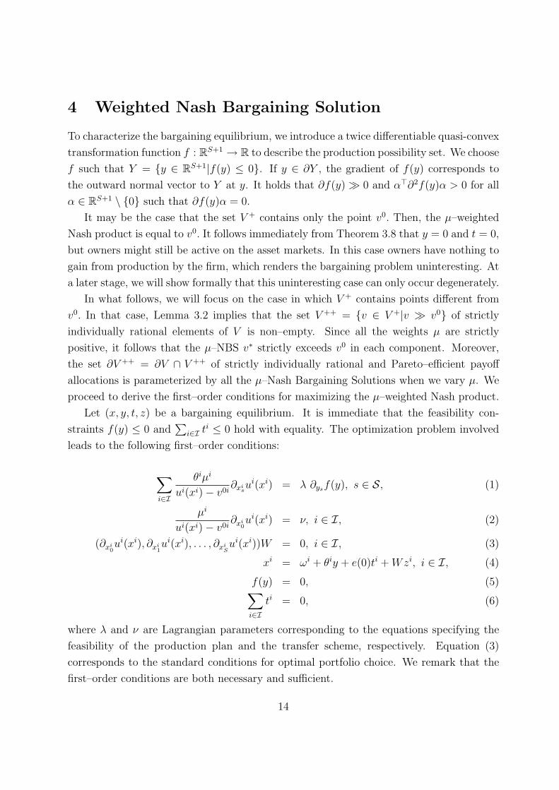
4 Weighted Nash Bargaining Solution
To characterize the bargaining equilibrium, we introduce a twice differentiable quasi-convex
transformation function f : RS+1 → R to describe the production possibility set. We choose
f such that Y = y ∈ RS+1|f(y) ≤ 0. If y ∈ ∂Y , the gradient of f(y) corresponds to
the outward normal vector to Y at y. It holds that ∂f(y) 0 and α>∂2f(y)α > 0 for all
α ∈ RS+1 \ 0 such that ∂f(y)α = 0.
It may be the case that the set V + contains only the point v0. Then, the µ–weighted
Nash product is equal to v0. It follows immediately from Theorem 3.8 that y = 0 and t = 0,
but owners might still be active on the asset markets. In this case owners have nothing to
gain from production by the firm, which renders the bargaining problem uninteresting. At
a later stage, we will show formally that this uninteresting case can only occur degenerately.
In what follows, we will focus on the case in which V + contains points different from
v0. In that case, Lemma 3.2 implies that the set V ++ = v ∈ V +|v v0 of strictly
individually rational elements of V is non–empty. Since all the weights µ are strictly
positive, it follows that the µ–NBS v∗ strictly exceeds v0 in each component. Moreover,
the set ∂V ++ = ∂V ∩ V ++ of strictly individually rational and Pareto–efficient payoff
allocations is parameterized by all the µ–Nash Bargaining Solutions when we vary µ. We
proceed to derive the first–order conditions for maximizing the µ–weighted Nash product.
Let (x, y, t, z) be a bargaining equilibrium. It is immediate that the feasibility con-
straints f(y) ≤ 0 and∑
i∈I ti ≤ 0 hold with equality. The optimization problem involved
leads to the following first–order conditions:
∑i∈I
θiµi
ui(xi)− v0i∂xi
sui(xi) = λ ∂ysf(y), s ∈ S, (1)
µi
ui(xi)− v0i∂xi
0ui(xi) = ν, i ∈ I, (2)
(∂xi0ui(xi), ∂xi
1ui(xi), . . . , ∂xi
Sui(xi))W = 0, i ∈ I, (3)
xi = ωi + θiy + e(0)ti +Wzi, i ∈ I, (4)
f(y) = 0, (5)∑i∈I
ti = 0, (6)
where λ and ν are Lagrangian parameters corresponding to the equations specifying the
feasibility of the production plan and the transfer scheme, respectively. Equation (3)
corresponds to the standard conditions for optimal portfolio choice. We remark that the
first–order conditions are both necessary and sufficient.
14

We denote the S-dimensional vector of marginal rates of substitution by ∇ui(xi), so
∇sui(xi) = ∂xi
sui(xi)/∂xi
0ui(xi) for s = 1, . . . , S. Similarly, we denote the S-dimensional
vector of marginal rates of transformation by ∇f(y), so ∇sf(y) = ∂ysf(y)/∂y0f(y) for
s = 1, . . . , S. When we substitute µi/(ui(xi)−v0i) = ν/∂xi0ui(xi) in the system of equations
(1), we find
ν = λ∂y0f(y),∑i∈I
θi∇ui(xi) = ∇f(y).
The last equality implies that the marginal rates of transformation vector is equal to the
θ–weighted average of the owners’ marginal rates of substitution vectors. Notice that due
to potential market incompleteness, it is not guaranteed that marginal rates of substitution
vectors are all equal or are equal to the marginal rate of transformation vector. Since the
marginal rate of transformation vector corresponds to the outward normal vector to Y at
y, we find that (1,∇f(y))y ≥ (1,∇f(y))y′ for all y′ ∈ Y, and therefore it holds that the
production plan chosen in a bargaining equilibrium maximizes
y0 +
(∑i∈I
θi∇ui(xi)
)y−0
over all production plans in Y. The corresponding objective function of the firm is known
as the Dreze criterion. We have thereby shown the following result.
Theorem 4.1 In a bargaining equilibrium, the production plan is chosen according to the
Dreze criterion.
For i ∈ I, for xi with ui(xi) > v0i, define ηi(xi) = ∂xi0ui(xi)/(ui(xi)− v0i). Then, (2) is
equivalent to
µiηi(xi) = ν, i ∈ I.
In Aumann and Kurz (1977), ηi(xi) is considered a measure of the owner’s boldness.
Consider a gamble where an owner i receives utility v0i with probability p and ui(xi+εe(0))
with probability 1 − p, where ε > 0. Let pi(xi, ε) be the maximum probability for which
owner i weakly prefers the gamble over consuming xi for sure. As pointed out in Roth
(1989), boldness corresponds to the maximum probability for which owner i is willing
to accept the gamble, per dollar of additional gains, when ε tends to zero. That is,
ηi(xi) = limε↓0 pi(xi, ε)/ε. Aumann and Kurz (1977) identify the point where boldness
15
is equal across all owners as the Nash Bargaining Solution. The above condition says
that a weighted Nash Bargaining Solution is the point where the product of boldness and
probability to propose is equal for all owners. In the special case where all owners have
the same probability to propose, it follows that at a bargaining equilibrium, all owners
have equal boldness. Although Aumann and Kurz (1977) define boldness in a context
with a single good, here we obtain a similar specification since only the marginal utility of
consumption in state 0 enters ηi(xi).
By definition of ∇ui(xi), we can write Equation (3) as
∇ui(xi)A = q, i ∈ I.
These are simply the conditions for optimal portfolio choice for each owner. When
markets are complete, for instance when A is the identity, marginal rate of substitution
vectors are all equal to each other and to the marginal rate of transformation vector.
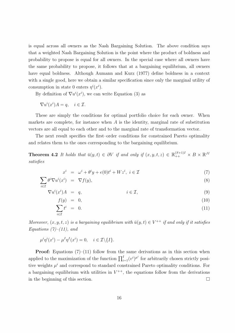
The next result specifies the first–order conditions for constrained Pareto optimality
and relates them to the ones corresponding to the bargaining equilibrium.
Theorem 4.2 It holds that u(y, t) ∈ ∂V if and only if (x, y, t, z) ∈ R(S+1)I++ × B × RJI
satisfies
xi = ωi + θiy + e(0)ti +Wzi, i ∈ I (7)∑i∈I
θi∇ui(xi) = ∇f(y), (8)
∇ui(xi)A = q, i ∈ I, (9)
f(y) = 0, (10)∑i∈I
ti = 0. (11)
Moreover, (x, y, t, z) is a bargaining equilibrium with u(y, t) ∈ V ++ if and only if it satisfies
Equations (7)–(11), and
µiηi(xi)− µIηI(xi) = 0, i ∈ I\I.
Proof: Equations (7)–(11) follow from the same derivations as in this section when
applied to the maximization of the function∏I
i=1(vi)µi
for arbitrarily chosen strictly posi-
tive weights µi and correspond to standard constrained Pareto optimality conditions. For
a bargaining equilibrium with utilities in V ++, the equations follow from the derivations
in the beginning of this section.
16
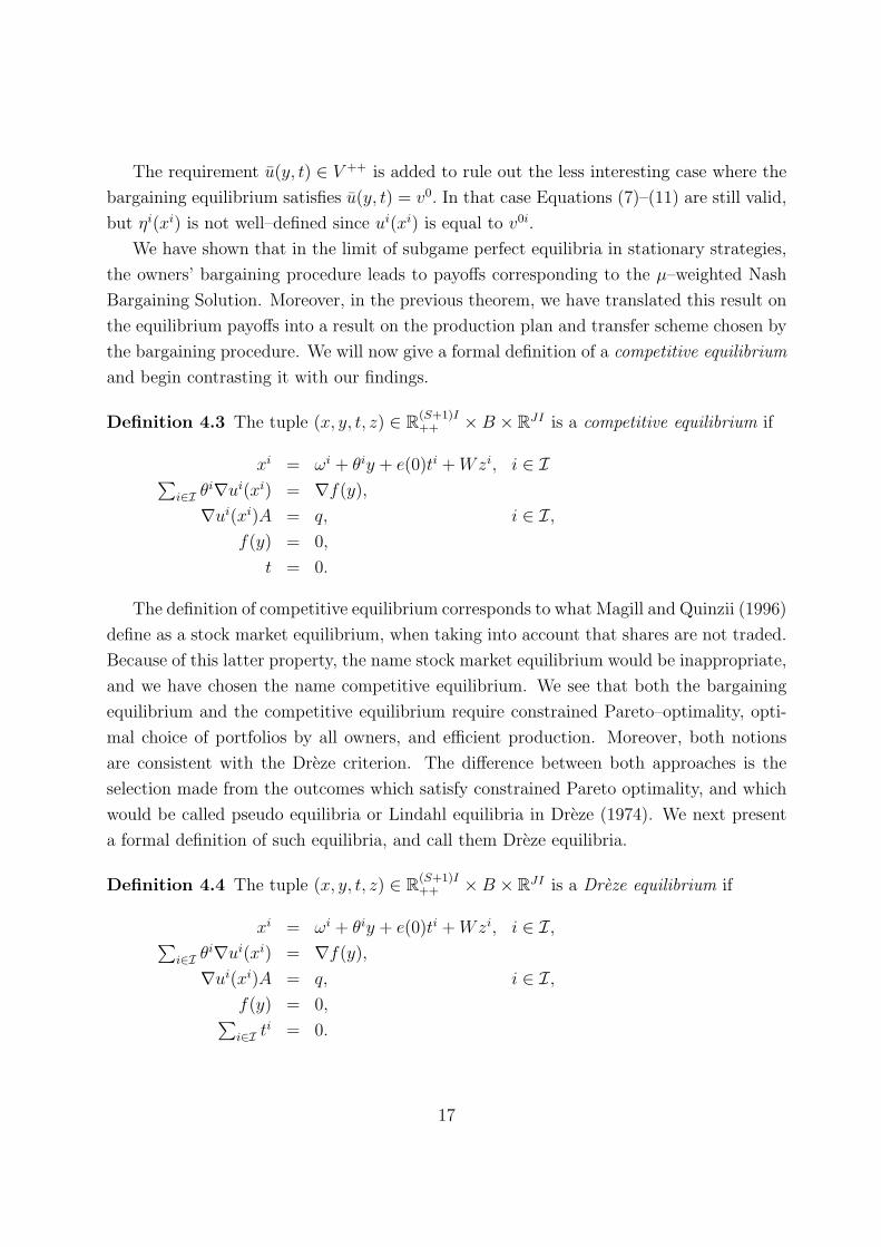
The requirement u(y, t) ∈ V ++ is added to rule out the less interesting case where the
bargaining equilibrium satisfies u(y, t) = v0. In that case Equations (7)–(11) are still valid,
but ηi(xi) is not well–defined since ui(xi) is equal to v0i.
We have shown that in the limit of subgame perfect equilibria in stationary strategies,
the owners’ bargaining procedure leads to payoffs corresponding to the µ–weighted Nash
Bargaining Solution. Moreover, in the previous theorem, we have translated this result on
the equilibrium payoffs into a result on the production plan and transfer scheme chosen by
the bargaining procedure. We will now give a formal definition of a competitive equilibrium
and begin contrasting it with our findings.
Definition 4.3 The tuple (x, y, t, z) ∈ R(S+1)I++ ×B × RJI is a competitive equilibrium if
xi = ωi + θiy + e(0)ti +Wzi, i ∈ I∑i∈I θ
i∇ui(xi) = ∇f(y),
∇ui(xi)A = q, i ∈ I,f(y) = 0,
t = 0.
The definition of competitive equilibrium corresponds to what Magill and Quinzii (1996)
define as a stock market equilibrium, when taking into account that shares are not traded.
Because of this latter property, the name stock market equilibrium would be inappropriate,
and we have chosen the name competitive equilibrium. We see that both the bargaining
equilibrium and the competitive equilibrium require constrained Pareto–optimality, opti-
mal choice of portfolios by all owners, and efficient production. Moreover, both notions
are consistent with the Dreze criterion. The difference between both approaches is the
selection made from the outcomes which satisfy constrained Pareto optimality, and which
would be called pseudo equilibria or Lindahl equilibria in Dreze (1974). We next present
a formal definition of such equilibria, and call them Dreze equilibria.
Definition 4.4 The tuple (x, y, t, z) ∈ R(S+1)I++ ×B × RJI is a Dreze equilibrium if
xi = ωi + θiy + e(0)ti +Wzi, i ∈ I,∑i∈I θ
i∇ui(xi) = ∇f(y),
∇ui(xi)A = q, i ∈ I,f(y) = 0,∑i∈I t
i = 0.
17

The competitive equilibrium chooses a Dreze equilibrium allocation which does not
require transfers. Bargaining power or the disagreement point play no role in this selection.
Under the bargaining equilibrium, one chooses the unique allocation which can be reached
by non–wasteful transfers and at which the µ–weighted boldness of all owners is equal.
Both the bargaining equilibrium and the competitive equilibrium are Dreze equilibria.
5 Producer Choice
We have studied the equilibrium production and transfer decision of the firm resulting
from the bargaining procedure. In the last section, we have characterized the outcome
of the bargaining procedure and given a first comparison to the competitive equilibrium.
In this section, we make use of the characterization given in Theorem 4.2 in order to
study the bargaining equilibrium in much more detail and explore its relation to important
concepts well–established in the literature, such as value–maximization and the competitive
equilibrium.
Any matrix of security payoffs W implies a set Π of (normalized) state prices. A
production plan is said to be value-maximizing if it is optimal with regard to some element
of Π (DeMarzo 1993). It turns out that the set of value-maximizing production plans is
closely related to the strictly individually rational Pareto–boundary of V , parameterized by
the weights µ of the Nash Bargaining Solution, which are in turn given by the recognition
probabilities of the bargaining procedure.
Definition 5.1 A production plan y ∈ Y is value–maximizing if there is a state price
vector π ∈ Π such that for all y ∈ Y,
πy ≤ πy.
In what follows, we show how our previous characterization of the µ-weighted NBS
relates to the value-maximization concept:
Lemma 5.2 A production plan y ∈ Y is value–maximizing if and only if it satisfies
∇f(y)A = q,
f(y) = 0.
Proof: This follows from the standard first–order conditions.
Theorem 4.2 and Lemma 5.2 imply that ∂V is supported only by production plans
which are value–maximizing. In the special case with complete markets, Π is single–valued
and value–maximization reduces to the usual profit–maximization.
18

Corollary 5.3 If S = J , then every v ∈ ∂V is supported by the profit–maximizing pro-
duction plan.
If markets are complete, the production decision of the firm in a bargaining equilibrium
is thus consistent with the usual profit–maximizing predictions of competitive equilibrium.
However, the distribution of bargaining power will determine how the firm’s profits are
to be divided among its owners. The bargaining equilibrium utilities may therefore differ
from the competitive equilibrium utilities even if markets are complete.
For the remainder of the section, we use the notation
uiss′ = ∂2ui(xi)/∂xis∂xis′ ,
∇sui(xi) = (∂ui(xi)/∂xis)/(∂u
i(xi)/∂xi0), s ∈ S\0,uiss′ = ∂ (∇su
i(xi)) /∂xis′ .
We summarize the second–order derivatives in matrices
U i =
ui00 ui01 · · · ui0Sui10 ui11 · · · ui1S...
.... . .
...
uiS0 uiS1 · · · uiSS
and U i =
ui10 ui11 · · · ui1S...
.... . .
...
uiS0 uiS1 · · · uiSS
.
Similarly, we write
fss′ = ∂2f(y)/∂ys∂ys′ ,
∇sf(y) = (∂f(y)/∂ys)/(∂f(y)/∂y0), s ∈ S\0,fss′ = ∂ (∇sf(y)) /∂ys′ .
and use the matrices
F =
f00 f01 · · · f0S
f10 f11 · · · f1S
......
. . ....
fS0 fS1 · · · fSS
and F =
f10 f11 · · · f1S
......
. . ....
fS0 fS1 · · · fSS
.
Theorem 5.4 The set of value–maximizing production plans is an (S − J)–dimensional
manifold.
19

Proof: We have to show that the matrix of partial derivatives of the following system
of equations
∇f(y)A− q = 0,
f(y) = 0,
has row rank J + 1 when evaluated at a solution y, after which the result follows from
counting equations and unknowns. To this end, we have to show that the rows of the
matrix(A>F
∂f(y)
)
are linearly independent. We first rewrite the entry in row j and column s′ of A>F as
follows:
[A>F ]s′
j =S∑s=1
Ajsfss′
=S∑s=1
Ajs
(fss′f0 − fsf0s′
(f0)2
)
=1
f0
[S∑s=1
Ajsfss′ −S∑s=1
Ajs∇sff0s′ ]
=1
f0
[S∑s=1
Ajsfss′ − qjf0s′ ]
= [1
f0
W>F ]s′
j .
The second line follows by applying the quotient rule, and the fourth line results from
∇f(y)A = q. Hence, we have that A>F = (1/f0)W>F . Now suppose by way of contradic-
tion that there is a row vector α ∈ RJ and β ∈ R with (α, β) 6= 0 such that
αA>F + β∂f(y) = 0.
From right-multiplication by W and ∂f(y)W = 0, we obtain αA>FW = 0. From right-
multiplication by α> and substitution of the previously derived expression for A>F , we
find that αW>FWα> = 0. Since f is differentiably quasi–convex, the last equation implies
∂f(y)Wα> 6= 0, contradicting the fact that ∂f(y)W = 0.
20

We have assumed that U i is negative definite, implying that it is of full rank. In order to
prove the next theorem, an important auxiliary result is that also the matrix of normalized
second–order derivatives U i has linearly independent rows. This is shown in the following
lemma.
Lemma 5.5 The matrix U i has linearly independent rows.
Proof: Suppose by way of contradiction that there is a row vector α ∈ RS\0 such
that αU i = 0. By definition of U i and the quotient rule
S∑s=1
αs
[uiss′
ui0− uisu
i0s′
(ui0)2
]= 0, s′ = 0, . . . , S,
so we have that
S∑s=1
αsuiss′ −
S∑s=1
αsuisui0ui0s′ = 0, s′ = 0, . . . , S.
Now define a vector α′ = (−∑S
s=1 αsui
s
ui0, α1, . . . , αS). Then,
∑Ss=0 α
′su
iss′ = 0, contradicting
the assumption that U i is negative definite.
Consider a particular v ∈ ∂V . If there exists a production plan y ∈ Y and asset
portfolios z1, . . . , zI such that ui(ωi + θiy + Wzi) = vi for all i ∈ I, then we say that the
point v is supported without transfers. Notice that competitive equilibria lead to points in
∂V which are supported without transfers.
In what follows, we will parameterize the economy by the initial endowments ω and the
bargaining weights µ. From now on, we will make this explicit by using the notation ∂Vω.
We state a number of results which all rely on a similar proof strategy. In each case, we
phrase the problem of interest in such a way that it amounts to finding the dimension of the
solution set of some system of equations. Each equation in this system can be identified
with the zero of a function in which the endowment schedule ω and/or the bargaining
weights µ are parameters, while the variables are production plans, transfer schemes, and
asset portfolios. We summarize the relevant partial derivatives of these functions with
respect to the parameters and the variables in a matrix, and prove that this matrix has
linearly independent rows. The parametric transversality theorem then implies that the
equations are linearly independent for almost all choices of the parameters. The pre–image
theorem is then invoked to find the dimension of the solution set.
An important auxiliary result is that, generically in ω, the disagreement point v0ω lies
in the interior of the bargaining set.
21

Lemma 5.6 There is an open set Ω∗ ⊂ R(S+1)I++ of full Lebesgue measure such that for all
endowments ω ∈ Ω∗, the payoff allocation v0ω which arises from the optimal portfolio choice
of all owners given no production and no transfers, does not belong to ∂V +ω .
Proof: Consider the following system of equations in ω and z, where ω ∈ R(S+1)I++ and
ωi +Wzi ∈ RS+1++ for all i ∈ I.∑
i∈I
θi∇ui(ωi +Wzi)−∇f(0) = 0, (12)
∇ui(ωi +Wzi)A− q = 0, i ∈ I, (13)
∇f(0)A− q = 0. (14)
It holds that v0ω ∈ ∂V +
ω if and only if (12)-(14) has a solution, as follows from the
characterization of the boundary in Theorem 4.2 by setting y = 0 and t = 0. We observe
that condition (14) is independent of ω. If (14) does not hold, then v0ω 6∈ ∂V +
ω . In particular,
by Assumption 2.3.3, condition (14) fails whenever markets are complete. Now consider
the case where condition (14) does hold, and hence S > J . Consider the derivatives of
conditions (12) and (13) above with respect to ωI , ω1, . . . , ωI−1, which can be written in
matrix form as
N =
θIU I θ1U1 · · · · · · θI−1U I−1
0 A>U1 0 · · · 0
0 0. . . 0 0
...... 0
. . . 0
0 0 · · · 0 A>U I−1
.
Lemma 5.5 and the full column rank of A imply that the diagonal blocks θIU I and
A>U i, i = 1, . . . , I − 1, have linearly independent rows. Therefore, the rows of N are
independent. By the parametric transversality theorem, this implies that the derivatives
of the aforementioned expressions with respect to z alone are linearly independent for
almost all ω ∈ R(S+1)I++ . Applying the pre-image theorem and counting unknowns and
equations, we find that the set of solutions to the above system is a manifold of dimension
J − S < 0 for almost all ω. We have shown that the set Ω∗ of endowments ω such that
v0ω 6∈ ∂V +
ω is of full Lebesgue measure. It holds that v0ω is a continuous function of ω,
and ∂V +ω is an upper-hemi-continuous correspondence in ω. Hence, if v0
ω 6∈ ∂V +ω for some
particular ω ∈ Ω∗, then v0ω 6∈ ∂V +
ω for all ω in a sufficiently small neighborhood of ω.
Therefore, Ω∗ is open, and the lemma follows.
22

Theorem 5.7 There is an open set P ∗ ⊂ R(S+1)I++ ×∆I of full Lebesgue measure such that
for all (ω, µ) ∈ P ∗, the bargaining equilibrium involves non–zero transfers.
Proof: We will introduce a system of equations in ω, µ , y, z, and z, where the variables
are restricted to satisfy the following conditions.
µi > 0, i ∈ I,ωi 0, i ∈ I,
ωi + θiy +Wzi 0, i ∈ I,ωi +Wzi 0, i ∈ I,
ui(ωi + θiy +Wzi)− ui(ωi +Wzi) > 0, i ∈ I.
The set of (ω, µ, y, z, z) satisfying these restrictions is open, and therefore a manifold.
The system of equations is as follows.
∇f(y)A− q = 0, (15)
f(y) = 0, (16)
∇ui(ωi + θiy +Wzi)A− q = 0, i ∈ I\I, (17)∑i∈I
θi∇ui(ωi + θiy +Wzi)−∇f(y) = 0, (18)
γ1(ω1, µ1, y, z1, z1)− γI(ωI , µI , y, zI , zI) = 0, (19)
∇ui(ωi +Wzi)A− q = 0, i ∈ I, (20)
where we have defined
γi(ωi, µi, y, zi, zi) =ui(ωi + θiy +Wzi)− ui(ωi +Wzi)
µi∂0ui(ωi + θiy +Wzi), i ∈ I.
Given (ω, µ), the solution to this system is a tuple (y, z, z) such that the production plan
y, the asset portfolios z, and zero transfers correspond to a µ-bargaining equilibrium with
v0ω ∈ ∂V +
ω and, moreover, z are asset portfolios corresponding to the disagreement point.
We want to show that for generically chosen (ω, µ), this system is over-determined. This
amounts to proving that the derivatives of the above equations are linearly independent.
Consider a block matrix M in which the first row corresponds to the J+1 derivatives of
equations (15)-(16), the second row to the IJ+S−J+1 derivatives of equations (17)-(19),
and the third row to the IJ derivatives of equation (20). Moreover, the first column gives
the derivatives with respect to y, the second column with respect to (ω, µ), and the third
23
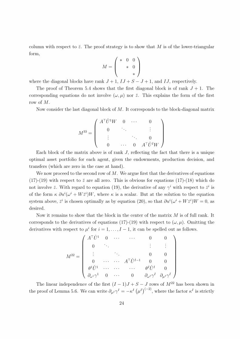
column with respect to z. The proof strategy is to show that M is of the lower-triangular
form,
M =
∗ 0 0
∗ 0
∗
where the diagonal blocks have rank J + 1, IJ + S − J + 1, and IJ , respectively.
The proof of Theorem 5.4 shows that the first diagonal block is of rank J + 1. The
corresponding equations do not involve (ω, µ) nor z. This explains the form of the first
row of M .
Now consider the last diagonal block of M . It corresponds to the block-diagonal matrix
M33 =
A>U1W 0 · · · 0
0. . .
......
. . . 0
0 · · · 0 A>U IW
Each block of the matrix above is of rank J , reflecting the fact that there is a unique
optimal asset portfolio for each agent, given the endowments, production decision, and
transfers (which are zero in the case at hand).
We now proceed to the second row of M . We argue first that the derivatives of equations
(17)-(19) with respect to z are all zero. This is obvious for equations (17)-(18) which do
not involve z. With regard to equation (19), the derivative of any γi with respect to zi is
of the form κ ∂ui(ωi + Wzi)W , where κ is a scalar. But at the solution to the equation
system above, zi is chosen optimally as by equation (20), so that ∂ui(ωi +Wzi)W = 0, as
desired.
Now it remains to show that the block in the center of the matrix M is of full rank. It
corresponds to the derivatives of equations (17)-(19) with respect to (ω, µ). Omitting the
derivatives with respect to µi for i = 1, . . . , I − 1, it can be spelled out as follows.
M22 =
A>U1 0 · · · · · · 0 0
0. . .
......
.... . . 0 0
0 · · · · · · A>U I−1 0 0
θ1U1 · · · · · · · · · θIU I 0
∂ω1γ1 0 · · · 0 ∂ωIγI ∂µIγI
The linear independence of the first (I − 1)J + S − J rows of M22 has been shown in
the proof of Lemma 5.6. We can write ∂µIγI = −κI(µI)(−2)
, where the factor κI is strictly
24

positive by the restriction that ui(ωi + θiy + Wzi) > ui(ωi + Wzi) for all i ∈ I. Also, we
have assumed µ 0, thus ∂µIγI < 0, as required.
We have now shown that the rows of M are linearly independent. By the parametric
transversality theorem, we can conclude that the set of (ω, µ) ∈ R(S+1)I++ × ∆I for which
the derivatives with respect to the remaining variables are linearly independent is of full
Lebesgue measure. By the preimage theorem, we may then count equations and unknowns
and find that the set of (ω, µ) ∈ R(S+1)I++ × ∆I for which the equation system is over-
determined is of full Lebesgue measure. Denote the intersection of that set with Ω∗ by
P ∗. If (ω, µ) ∈ P ∗, then the bargaining equilibrium involves non-zero transfers. P ∗ is
of full Lebesgue measure. Moreover, the (unique) bargaining equilibrium is a continuous
function of (ω, µ). Therefore, if the property of non-zero transfers holds for some (ω, µ) ∈R(S+1)I
++ ×∆I , then it also holds for (ω, µ) ∈ R(S+1)I++ ×∆I in a sufficiently small neighborhood
of (ω, µ). Hence, the set P ∗ is open.
Theorem 5.7 says that generically in endowments and bargaining weights the bargain-
ing procedure will lead to transfers. Since competitive equilibria involve zero transfers,
bargaining equilibria are generically distinct from competitive equilibria.
Corollary 5.8 There is an open set P ∗ ⊂ R(S+1)I++ ×∆I of full Lebesgue measure such that
for all (ω, µ) ∈ P ∗, the bargaining equilibrium is not a competitive equilibrium.
Since by Theorem 3.8 points in ∂V + are supported by uniquely defined production plans
and transfer schemes, the bargaining equilibrium utilities and the competitive equilibrium
utilities are different for almost all endowments and bargaining weights.
Corollary 5.9 There is an open set P ∗ ⊂ R(S+1)I++ × ∆I of full Lebesgue measure such
that for all (ω, µ) ∈ P ∗, the bargaining equilibrium utilities are not equal to competitive
equilibrium utilities.
This difference in payoff allocation holds for both complete and incomplete markets.
In the case of complete markets, we have previously shown that the profit-maximizing
production plan is selected by the bargaining procedure. Thus, with complete markets,
any difference in payoff allocation must be due to the transfers. With regard to incomplete
markets, however, we will show in the sequel of this section that the difference in payoff
allocation is not only the result of transfers, but that the chosen production plan is different
as well.
25

Theorem 5.10 Suppose that markets are incomplete, that is, J < S. Then, there is an
open set P ∗∗ ⊂ R(S+1)I++ × ∆I of full Lebesgue measure such that for all (ω, µ) ∈ P ∗∗, the
bargaining equilibrium production plan is not a competitive equilibrium production plan.
Proof: We introduce a system of equations in (ω, µ), y, t, z, z, and z, where the
variables are restricted as follows.
µi > 0, i ∈ I,ωi 0, i ∈ I,
ωi + θiy + e(0)ti +Wzi 0, i ∈ I,ωi + θiy +Wzi 0, i ∈ I,
ωi +Wzi 0, i ∈ I,ui(ωi + θiy + e(0)ti +Wzi)− ui(ωi +Wzi) > 0, i ∈ I.
The set of variables satisfying these restrictions is open, and is therefore a manifold.
The system of equations under consideration is as follows.
∑i∈I
ti = 0, (21)
∇f(y)A− q = 0, (22)
f(y) = 0, (23)
∇ui(ωi + θiy + e(0)ti +Wzi)A− q = 0, i ∈ I\I, (24)∑i∈I
θi∇ui(ωi + θiy + e(0)ti +Wzi)−∇f(y) = 0, (25)
γi(ωi, µi, y, ti, zi, zi)− γI(ωI , µI , y, tI , zI , zI) = 0, i ∈ I\I, (26)
∇ui(ωi + θiy +Wzi)A− q = 0, i ∈ I\I, (27)∑i∈I
θi∇ui(ωi + θiy +Wzi)−∇f(y) = 0, (28)
A>∇ui(ωi +Wzi)− q = 0, i ∈ I. (29)
In words, the equations specify that –given (ω, µ)– (y, t, z) is the µ-bargaining equi-
librium, and (y, 0, z) is the competitive equilibrium, where for i ∈ I, we have xi =
ωi + θiy + e(0)ti + Wzi and xi = ωi + θiy + Wzi. We want to show that for generi-
cally chosen (ω, µ), this system is over-determined whenever markets are complete. This is
equivalent to proving that the equations in the system above are all linearly independent.
26

Let N be a matrix where the first row corresponds to the derivative of equation (21),
the second row corresponds to the J + 1 derivatives of equations (22)-(23), the third row
corresponds to IJ + S − J + I − 1 derivatives of equations (24)-(26), the fourth row to
the IJ + S − J derivatives of equations (27)-(28) and the fifth row corresponds to the IJ
derivatives of equation (29). Moreover, the first column refers to derivatives with respect
to t, the second column with respect to y, the third column with respect to (ω, µ), the
fourth column with respect to z, and the fifth column with respect to z.
We will show that N is of the lower triangular form,
N =
∗ 0 0 0 0
∗ 0 0 0
∗ 0 0
∗ 0
∗
,
where the diagonal blocks are of full row rank 1, J + 1, IJ +S−J + I−1, IJ +S−J , and
IJ , respectively. By the parametric transversality theorem, this means that for generic
(ω, µ), the matrix of derivatives with respect to the remaining variables (y, z, z, z, t) has
linearly independent rows. Applying the pre-image theorem, this will imply that the set
of (y, z, z, z, t) which solve the above equation system given a generic (ω, µ) is a manifold
of dimension J − S, and corresponds therefore to the empty set when J < S.
Equation (21) involves only t, which explains the form of the first row of N . Equations
(22)-(23) involve only y. This together with Theorem 5.4 explains that the second row
of N is of the form indicated above. The linear independence of the IJ rows in the last
diagonal block of N follows by the same argument as in the proof of Theorem 5.7. Aside
from equation (29), the portfolios z are only involved in equation (26). But the derivative
of (26) with respect to z must be zero at the solution to the equation system, whence
the zero entries in the fifth column of N – the argument is as in the proof of Theorem
5.7. Similarly, the portfolios z are involved only in equations (27)-(28), explaining the zero
entries in the fourth column of N .
Consider the third diagonal block of N . After appropriate permutations of the rows
and columns, it can be spelled out as follows.
27

N33 =
A>U1 0 · · · · · · 0 0 0 0 0 0
0. . .
......
......
......
.... . . 0
......
......
...
0 · · · · · · A>U I−1 0...
......
......
θ1U1 · · · · · · · · · θIU I 0 0 0 0 0
∂ω1γ1 0 · · · 0 ∂ωIγI ∂µ1γ1 0 · · · 0 ∂µIγI
0. . .
... 0. . .
......
.... . .
......
. . . 0...
0 · · · 0 ∂ωI−1γI−1 ∂ωIγI 0 · · · 0 ∂µI−1γI−1 ∂µIγI
The block in the upper left corner has previously been shown to be of rank IJ+S−J , see
the proof of Lemma 5.6. We have argued in the proof of Theorem 5.7 that the terms of the
form ∂µiγi are strictly positive, which readily implies the full rank I− 1 of the block in the
lower right corner. Let P ∗∗ be the intersection of Ω∗ with the set of all (ω, µ) ∈ R(S+1)I++ ×∆I
for which the matrix under consideration has linearly independent rows. We have shown
that P ∗∗ is of full Lebesgue measure. The bargaining equilibrium is a continuous function
of (ω, µ), and the competitive equilibria are an upper-hemi-continuous correspondence of
(ω, µ). If the property of strictly positive distance between the bargaining and competitive
equilibrium production plans holds for some (ω, µ) ∈ R(S+1)I++ ×∆I , then it is preserved for
(ω, µ) ∈ R(S+1)I++ ×∆I in a sufficiently small neighborhood around (ω, µ).
We had previously shown that generically in endowments and bargaining weights the
payoff allocation resulting from the bargaining equilibrium and that resulting from a com-
petitive equilibrium are different. We have seen that in the case of complete markets, the
production plan chosen under both approaches is the same, so that the different payoff
allocation is merely a result of redistribution via transfers. The last theorem complements
these findings by saying that for the case of incomplete markets, the two approaches almost
always lead to different production plans.
6 Conclusion
We have introduced a non–cooperative bargaining procedure to resolve the conflict among
shareholders of a firm when markets are incomplete. In contrast to many existing models,
we obtain a unique prediction for the production plan as well as for the resulting payoff
28

allocation. This solution is parameterized by the distribution of bargaining power across
the different owners. This bargaining power distribution is independent of the shares of
ownership.
An important feature of the model is that transfers are possible in equilibrium. The
well–known Dreze criterion rules out a production plan which can be Pareto–improved
upon by an alternative plan and transfers. The well–known solution concept of a stock
market equilibrium satisfies this criterion but requires that the chosen production plan
itself should be implemented without transfers. Our solution concept, called a bargaining
equilibrium, satisfies the Dreze criterion but does allow for transfers to be made in equi-
librium. Indeed, it turns out that transfers will almost always be used. Furthermore, the
bargaining equilibrium is derived from an explicit non–cooperative bargaining model. The
outcome of the bargaining procedure proposed in this paper is different from the predic-
tions of standard economic theory. If markets are complete, the production decision of the
firm is driven by profit–maximization as in the Arrow–Debreu model. However, the profits
are redistributed among the owners of the firm in accordance with their bargaining power,
which derives from the ability to make a proposal and from the disagreement payoff. In the
case of incomplete markets, the production plan adopted under the bargaining procedure
almost always fails to be a competitive equilibrium production plan. Non–zero transfers
are almost always made. We have given positive support for the use of the Dreze criterion,
though the utility gradients of owners implied by our theory differ from the competitive
equilibrium ones.
In our bargaining game we have not considered the option for owners to modify owner-
ship shares and/or to sell the firm to outsiders. An intriguing question for future research is
whether allowing such possibilities would give support for the criterion proposed by Bisin,
Gottardi and Ruta (2009), which loosely speaking corresponds to the maximal utility gra-
dient in the population rather than a weighted average of the owner’s utility gradients as
a criterion.
29

References
Aumann, R.J., and M. Kurz (1977), “Power and Taxes,” Econometrica, 45, 1137–1161.
Bisin, A., P. Gottardi, and G. Ruta (2009), “Equilibrium Corporate Finance,” WorkingPaper, European University Institute.
Bonnisseau, J.-M., and O. Lachiri (2004), “On the Objective of Firms under Uncertaintywith Stock Markets,” Journal of Mathematical Economics, 40, 493–513.
Britz, V., P.J.J. Herings, and A. Predtetchinski (2010), “Non-cooperative Support forthe Asymmetric Nash Bargaining Solution,” Journal of Economic Theory, 145, 1951–1967.
DeMarzo, P. (1993), “Majority Voting and Corporate Control: The Rule of the DominantShareholder,” Review of Economic Studies, 60, 713–734.
Diamond, P.A. (1967), “The Role of a Stock Market in a General Equilibrium Model withTechnological Uncertainty,” American Economic Review, 57, 759–776.
Dierker, E., H. Dierker, and B. Grodal (2002), “Nonexistence of Constrained EfficientEquilibria When Markets Are Incomplete,” Econometrica 70, 1245–1251.
Dreze, J.H. (1974), “Investment under Private Ownership: Optimality, Equilibrium, andStability,” in J.H. Dreze, ed., Allocation under Uncertainty: Equilibrium and Optimality(New York: Macmillan, 1974) 9.
Dreze, J.H., O. Lachiri, and E. Minelli (2009), “Stock Prices, Anticipations and Invest-ment in General Equilibrium,” CORE Discussion Paper, 2009/83, 1–46.
Grossman, S.J., and O. Hart (1979), “A Theory of Competitive Equilibrium in StockMarket Economies,” Econometrica, 47, 293–330.
Hart, S. and A. Mas-Colell (1996), “Bargaining and Value,” Econometrica, 64, 357–380.
Kelsey, D., and F. Milne (1996), “The Existence of Equilibrium in Incomplete Markets andthe Objective Function of the Firm,” Journal of Mathematical Economics, 25, 229–245.
Laruelle, A., and F.Valenciano (2007), “Bargaining in Committees as an Extension ofNash’s Bargaining Theory,” Journal of Economic Theory, 132, 291-305.
Magill, M., and M. Quinzii (1996), Theory of Incomplete Markets, MIT Press, Cambridge,Massachusetts.
Miyakawa, T. (2008), “Noncooperative Foundation of n-Person Asymmetric Nash BargainingSolution,” Journal of Economics of Kwansei Gakuin University, 62, 1–18.
Rockafellar, R.T. (1970), Convex Analysis, Princeton University Press, Princeton, NewJersey.
Roth, A.E. (1989), “Risk Aversion and the Relationship between Nash’s Solution and Sub-game Perfect Equilibrium of Sequential Bargaining,” Journal of Risk and Uncertainty, 2,353–365.
30

Tvede, M., and H. Cres (2005), “Voting in Assemblies of Shareholders and IncompleteMarkets,” Economic Theory, 26, 887–906.
31


