United StatesDepartment ofAgriculture
Forest Service
ForestProductsLaboratory
ResearchPaperFPL-RP-493
Two- and Three-Parameter WeibullGoodness-of-Fit Tests
James W. EvansRichard A. JohnsonDavid W. Green

Abstract
Research Highlights
Extensive tables of goodness-of-fit critical values for the two- and three-parameter Weibulldistributions are developed through simulation for the Kolmogorov-Smirnov statistic, theAnderson-Darling statistic, and Shapiro-Wilk-type correlation statistics. Approximating formulasfor the critical, values are derived and compared with values in the tables. Power studies usingseveral different distributional forms show that the Anderson-Darling statistic is the mostsensitive to lack of fit of a two-parameter Weibull and correlation statistics of the Shapiro-Wilktype the most sensitive to departures from a three-parameter Weibull.
Keywords: Goodness-of-fit statistics, Weibull distribution, lumber strength, modulus of elasticity
This paper presents the results of a study to develop and evaluate goodness-of-fit tests for thetwo- and three-parameter Weibull distributions. The study was initiated because of discrepanciesin published critical values for two-parameter Weibull distribution goodness-of-fit tests, the lackof any critical values for a Shapiro-Wilk-type correlation statistic, and the lack of generalthree-parameter Weibull distribution goodness-of-fit tests. The results of the study will be usedby Forest Products Laboratory (FPL) scientists to evaluate the goodness-of-fit of Weibulldistributions to experimental data. This will allow evaluation of distributional forms that may beused in reliability-based design procedures.
Through computer simulation, extensive tables of critical values for three standardgoodness-of-fit statistics are developed for both the two- and three-parameter Weibulldistributions. The statistics used are the Kolmogorov-Smirnov D statistic, the Anderson-DarlingA2 statistic, and a Shapiro-Wilk-type correlation statistic. The critical values for the statistics aremodeled through regression to provide equations to estimate the critical values. The equationsallow computer programs to evaluate the goodness-of-fit of data sets containing up to 400observations. The abilities of the tests to detect poor fits (the “power of the tests”) are studiedusing both the equations and the exact critical values of the test statistics. Finally, invarianceproperties of the statistics are proved. These invariance properties show that the scope of thesimulation is adequate for all problems that the tests might be applied to.
Four general conclusions are readily apparent from the results of this study:
1. Of the three statistics considered, the Anderson-Darling A2 statistic appears to be the statisticof choice for testing the goodness-of-fit of a two-parameter Weibull distribution to a set ofdata. The choice might be different if censored data were used since the correlation statistichas the potential advantage of being easily modified for type I and type II censoredobservations.
2. For testing the three-parameter Weibull goodness-of-fit, the correlation statisticsappear to be the best.
3. The critical value approximations appear to be very good for the range of sample sizesconsidered.
4. The power of the tests is very dependent upon the true distributional form of the data.
November 1989
Evans, James W.; Johnson, Richard A.; Green, David W. Two- and three-parameter Weibull goodness-of-fittests. Res. Pap. FPL-RP-493. Madison, WI: U.S. Department of Agriculture, Forest Service, ForestProducts Laboratory; 1989. 27 p.
A limited number of free copies of this publication are available to the public from the Forest ProductsLaboratory, One Gifford Pinchot Drive, Madison, WI 53705-2398. Laboratory publications are sent to morethan 1,000 libraries in the United States and elsewhere.
The Forest Products Laboratory is maintained in Madison, Wisconsin, by the U.S. Department ofAgriculture, Forest Service, in cooperation with the University of Wisconsin.
Two- and Three-Parameter WeibullGoodness-of-Fit Tests
James W. Evans, Supervisory Mathematical StatisticianUSDA Forest ServiceForest Products LaboratoryMadison, Wisconsin
Richard A. Johnson, ProfessorDepartment of StatisticsUniversity of WisconsinMadison. Wisconsin
David W. Green, Research General EngineerUSDA Forest ServiceForest Products LaboratoryMadison, Wisconsin
Background andIntroduction
Two-parameter and three-parameter Weibull distributions are widely used to representthe strength distribution of structural lumber and engineering-designed woodsubassemblies. As wood construction practices in the United States and Canada arerevised from deterministic to reliability-based design procedures, assessing thegoodness-of-fit of these Weibull distributional forms becomes increasingly important.In its three-parameter form, the family is represented by the density function
(1)
where a is the shape parameter, b the scale parameter, and c the location parameter.The family of two-parameter Weibull distributions follows from Equation (1) whenc = 0.
Goodness-of-fit tests for the two-parameter Weibull distributions have receivedconsiderable attention. Mann and others (1973), Smith and Bain (1976), Stephens(1977), Littell and others (1979), Chandra and others (1981), Tiku and Singh (1981),and Wozniak and Warren (1984) have all discussed aspects of this problem. Mann andothers (1973) and Tiku and Singh (1981) proposed new statistics to test thegoodness-of-fit of two-parameter Weibull distributions. Smith and Bain (1976)proposed a test statistic analogous to the Shapiro-Francis statistic for testingnormality. The Smith and Bain T statistic was based on the sample correlation betweenthe order statistics of a sample and the expected value of the order statistics under theassumption that the sample comes from a two-parameter Weibull distribution. Forcomplete samples and two levels of censoring, they provided critical values for samples

containing 8, 20, 40, 60, or 80 observations. Stephens (1977) produced tables of theasymptotic critical values of the Anderson-Darling A2 statistic and the Cramer-von Mises W 2 statistic for various significance levels. Littell and others (1979) comparedthe Mann, Scheuer, and Fertig S statistic, the Smith and Bain T statistic, the modifiedKolmogorov-Smirnov D statistic, the modified Cramer-von Mises W2 statistic, and themodified Anderson-Darling A2 statistic through a series of power studies for samplesize n = 10 to 40. They also calculated critical values for the D, W 2 , and A2 statisticsfor n = 10, 15, . . . , 40. Chandra and others (1981) calculated critical values for theKolmogorov-Smirnov D statistic for n = 10, 20, 50, and infinity for three situations.
The three-parameter Weibull distribution has received considerably less attention,probably because the critical values depend upon the unknown shape parameter.Woodruff and others (1983) produced tables of critical values for a modifiedKolmogorov-Smirnov test for a Weibull distribution with unknown location and scaleparameters and a known shape parameter. Their tables included n = 5 to 15, 20, 25,and 30 for shape parameters of 0.5, 1.0, . . . , 4.0. Bush and others (1983) producedsimilar tables for the Cramer-von Mises and Anderson-Darling statistics, together witha relationship between the critical value and the inverse shape parameter. Noasymptotic results or Monte Carlo determinations for n > 30 appear in the literature.
Despite this extensive literature, we encountered difficulties when we studied thegoodness-of-fit of two- and three-parameter Weibull distributions to numerous datasets consisting of 80 to 400 observations of various lumber strength properties. For thethree-parameter Weibull tests, critical values are not published for the sample sizesinvolved, and it is not clear how estimated shape parameters would affect the criticalvalues derived by assuming a known shape parameter. For the two-parameter Weibulltests, these difficulties included a lack of published critical values for sample sizeslarger than 50 and some apparent inconsistencies in published critical values. Theseapparent inconsistencies can be seen in our Tables 1 and 2. In Table 1 the Chandra andothers (1981) and the Littell and others (1979) critical values for the Kolmogorov-Smirnov D statistic show generally good agreement. (We scaled Littell’s values tocompare with Chandra’s by multiplying the test statistic critical value by n1 / 2.)However, Littell and others (1979) might have obtained a smoother set of values if theyhad used a larger simulation. Some inconsistencies at the 0.01 level of significance arealso evident. Since Littell and others (1979) reported the means of 10 runs of 1,000simulations and Chandra and others (1981) performed one run of 10,000, the lattervalues might be expected to be smoother at the 0.01 level. Wozniak and Warren (1984)calculated critical values for the Anderson-Darling statistic for the two-parameterWeibull distribution when parameters are estimated by maximum likelihood. Acomparison of their results with those of Stephens (1977) and Littell (Table 2) showssome variability in the second decimal of the critical values. For example, the Stephenscritical value at the 0.05 level for n = 40 is the same as the Wozniak and Warren0.05-level value for n = 15. The Littell value for n = 15 is even larger than theWozniak value.
In this paper, we (1) develop extensive and definitive two-parameter Weibulldistribution goodness-of-fit critical values for the Shapiro-Wilk-type correlationcoefficient statistics, the Anderson-Darling A2 statistic, and the Kolmogorov-SmirnovD statistic, (2) develop and evaluate formulas to yield a smoothed estimate of thecritical values for the statistics, and (3) extend these three statistics for use asgoodness-of-fit statistics with a three-parameter Weibull distribution.
2

Shapiro-Wilk-TypeCorrelation Statistic
Studies such as the Monte-Carlo study of Shapiro and others (1968) have consistentlyshown that for testing goodness-of-fit of normal distributions, the Shapiro-Wilkstatistic has superior power to other statistics in detecting that the data comes from awide range of other distributions. To develop a similar goodness-of-fit test for Weibulldistributions, we modify a simplified form of this statistic first suggested by Shapiroand Francia (1972) but with approximate “scores” suggested by Filliben (1975).
Let X(1) , X(2 ) , . . . , X ( n ) denote an ordered sample of size n from the population ofinterest. Specifically, for the two- and three-parameter Weibull distribution, weconsider the test statistic where
(2)
and
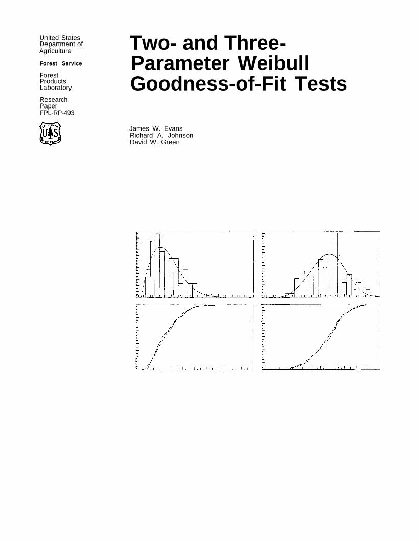
is a median score, in the spirit of Filliben, except that these scores depend upon themaximum likelihood estimate of the Weibull shape parameter a. The correspondingQ-Q plot of (X( i ), m w , i) should resemble a straight line if the underlying population isWeibull. (A Q-Q plot is an abbreviated notation for a Quantile-Quantile probabilityplot, where corresponding percentiles of one distribution are plotted against thepercentiles of the other, as discussed in Wilk and Gnanadesikan (1968).) The statistic
is the squared correlation coefficient of this plot. Note that the choice of m w , i
follows the approximate scores suggested by Filliben (1975) and is slightly differentfrom that chosen by Smith and Bain (1976).
If a variable X has the two-parameter Weibull distribution, the variable Y = ln X hasan extreme value distribution. Calculating goodness-of-fit on this scale has advantages.Since the extreme value distributions are defined by location and scale parameters, thecritical values for the correlation statistic are not dependent on the true shapeparameter. Thus, for two-parameter Weibull distributions, we propose thecorrelation-type statistic where
(3)
and
OtherGoodness-of-FitStatistics
We include two other well-studied goodness-of-fit statistics for comparative purposes.The modified Komogorov-Smirnov D statistic is given by
where Fn (x) is the empirical distribution function of the sample and F(x;b,a) is thefitted distribution.
3

The modified Anderson-Darling A2 statistic is given by
where U( i ) = F(X ( i ) ;b,a) and X( i ) is the ith-order statistic.
Unlike the statistic, neither D nor A2 is affected by the choice of scale. Thus, wecan use either X or ln X in the calculations.
Two-Parameter Simulation ResultsWeibullDistributions
The results of David and Johnson (1948) imply that the distributions of D and A 2 donot depend upon the values of b and a. Similarly, the distribution of does notdepend upon the values of b and a. These and some other invariance properties of thestatistics are shown in the Appendix. Therefore, without loss of generality, thedistributions of D, A2 , and can be obtained assuming b = 1 and a = 3.6.
To calculate the critical values of the statistics, we used IMSL (1979) to generate afixed sample U( 1 ) , U (2), . . . , U( n ) of n order statistics from a uniform distribution.Then we transformed to the Weibull order statistics,
where b = 1 and a = 3.6. The sample X( 1 ) , X (2), . . . , X ( n ) was used to calculatemaximum likelihood estimates of b and a. Finally we calculated D, A2 , and for thesample of size n. Values of n = 10, 1.5, . . . , 50; n = 60, 70, . . . , 100; n = 120,140, . . . , 200; and n = 240, 280, . . . , 400 were used. Concern over the apparentvariability of results for the Anderson-Darling critical values led us to try severalpreliminary simulations with 1,000 to 10,000 replications. Results confirmed that thetype of variability seen in Table 2 could occur from one simulation to the next.Because we were interested in smoothing out irregularities found in other tables, wegenerated 50,000 values for each goodness-of-fit statistic. These 50,000 values wereranked, and the 80th, 85th, 90th, 95th, and 99th percentiles were determined. Thevalues in Table 3 are the results of this simulation. For the Kolmogorov-SmirnovD statistic, as in Chandra and others (1981), we again multiplied the critical value byn1 / 2. By repeating the simulation with a different set of 50,000 replications for varioussample sizes, we determined that extending the simulation to 50,000 replicationsreduces the variability in the Anderson-Darling A2 statistic critical values from thesecond to the third decimal point. This is important for n > 50 because the criticalvalues become much closer together.
Critical Value Approximations
In an effort to smooth the critical values in Table 3 and simplify future use of the teststatistics, we modeled the critical values as functions of sample size. The modelingresulted in the following separate equations for the critical values of theKolmogorov-Smirnov D statistic at the 0.10, 0.05, and 0.01 levels of significance:
4
These curves fit the tabled values reasonably well, as shown in Figure 1. We made noattempt to force these curves to give the asymptotic values of Chandra and others(1981). Those asymptotic values were estimated by an extrapolation proceduredescribed in their paper. Since the critical values in Table 3 are slightly above theestimated asymptotic values for large samples, we decided to fit the data of Table 3without forcing the curve through Chandra’s estimate.
Stephens’ (1977) modification of the asymptotic critical values of the Anderson-DarlingA2 statistic for use with finite samples requires multiplying the value found by the teststatistic by (1 + 0.2/n1/2). The resulting value can then be compared to the asymptoticcritical values shown in Table 2. Results of this procedure are plotted in Figure 2. Herethe critical values in Table 3 are converted and compared to the asymptotic values.Figure 2 shows that the approximation is very good.
Modeling the critical values of the correlation statistic produces the followingseparate equations for the 0.10, 0.05, and 0.01 levels of significance:
These curves are plotted with the critical values in Figure 3.
Power Studies
To evaluate our results, we conducted a power study of the three statistics, D, A2, andusing four different distributions:
1. Uniform distribution on 0 to 1
2. Truncated normal with a mean of 1.4 and standard deviation of 0.35 (Thedistribution is truncated so that no values less than 0.00001 are allowed.)
3. Lognormal distribution where In X has a mean of 1.6 and standard deviation of 0.4
4. Gamma distribution with shape parameter equal to 2 and scale parameter equal to 1
The procedure involved generating 5,000 pseudorandom samples of size n from each ofthe four alternative distributions considered. We then calculated each of the three teststatistics and compared them to their critical values from Table 3 and the
5

approximations to the critical values obtained from the equations for D, A2, andIn each case, we counted the number of rejections of the null hypothesis. We repeatedthis procedure for sample sizes of n = 20, 50, 80, 100, and 200.
Results of the power study are presented in Tables 4 to 6, which show that theAnderson-Darling A2 statistic is generally superior to (that is, has a larger power than)both the Kolmogorov-Smirnov D and the correlation statistics for the alternativespresented. Neither D nor appears to be very powerful across this group ofalternative distributions. One other feature illustrated in Tables 4 to 6 is the closeagreement in power between the actual critical values and the values from theapproximation formulas, which attests to the accuracy of the approximations.

Three-ParameterWeibullDistributions
Simulation Results
Developing critical values for the three-parameter Weibull distribution goodness-of-fitcritical statistics is more difficult because they depend upon the unknown shapeparameter. Selecting the scale on which to perform the tests is also a problem. In thetwo-parameter case, using In X(i) instead of X(i) made the correlation statisticindependent of the shape parameter. In the three-parameter case, the choice of whichscale to use is not obvious. For the Kolmogorov-Smirnov D and the Anderson-DarlingA2 statistics, the two scales produce the same results. Therefore, we investigated D, A2 ,
and using a = 2.0, 2.8, 3.6, 4.4, and 5.2. We chose b = 1.0 and c = 2.0.Invariance properties derived in the Appendix show that the critical values of thestatistics depend only upon the shape parameter.
To calculate the critical values of the statistics, IMSL (1979) routines were again usedto generate a fixed sample U( 1 ) , U ( 2 ) , . . . , U(n) of n order statistics from a uniformdistribution. Then we transformed to the Weibull order statistics,
for the different combinations of a, b, and c. Maximum likelihood estimates of a, b,and c were calculated for the sample X(1), X(2), . . . , X(n),. Finally we calculated D,A2 , and for the sample of size n. Values of n = 20, 40, . . . , 200 were used.Because of the increased computer time required to calculate the maximum likelihoodestimates for the three-parameter Weibull distribution compared with thetwo-parameter case, it was possible to do only 10,000 replications. Thus, for eachsample size and choice of a, b, and c, 10,000 data sets were created and thegoodness-of-fit statistics evaluated. For each statistic, the 10,000 values were rankedand the 80th, 85th, 90th, 95th and 99th percentiles were determined (Tables 4 to 10).Again the results for the Kolmogorov-Smirnov statistic have been multiplied by n 1 / 2 .
7

Critical Value Approximations
We wanted to smooth the results and develop formulas that would approximate thecritical values. Because the critical values vary slightly for different shape parameters,two models were tried for each statistic. One model ignores the differences in valuesdue to shape and just expresses the general trend due to sample size. For this simplemodel, we determined that for the Kolmogorov-Smirnov D statistic and theAnderson-Darling A2 statistic, the two-parameter models could be modified bysubtracting a constant from the two-parameter model for the critical value. For thecorrelation statistics, producing an entirely new model was better. A second model,more complex, attempts to model the apparent quadratic nature of the effect of shapeon the critical values. This refinement was added to the simple model developed foreach of the three statistics. Thus, two models were created to predict the critical valuesof the Kolmogorov-Smirnov, Anderson-Darling, and correlation (original and extremevalue scales) statistics.
Kolmogorov-Smirnov Models –
1. Two-parameter model plus a shift
2. Two-parameter model plus a shift and an adjustment for the estimated shapeparameter values (labeled SHAPE in the formulas)
Testing is done by multiplying the Kolmogorov-Smirnov D statistic by n1 / 2 andcomparing the result to the critical values from the formulas. We reject the hypothesisthat a three-parameter Weibull fits the data if n 1 / 2 (D) is larger than the critical value.
Anderson-Darling Models –
1. Two-parameter model plus a shift
8
2. Two-parameter model plus a shift and an adjustment for shape
Testing is done by multiplying the Anderson-Darling A2 statistic by (1.0 + 0.2/n 1 / 2)and comparing to the critical values from the formulas. We reject the hypothesis that athree-parameter Weibull fits the data if A2 (1 + 0.2/n1 / 2) is larger than the criticalvalue.
Correlation Models – Original Scale –
1. New models
2. New models plus an adjustment for shape
Testing is done by comparing calculated using X( i ) to the critical values from theformulas. We reject the hypothesis that a three-parameter Weibull fits the data if i sless than the critical value.
Correlation Models-Extreme Value Scale –
1. New models
9
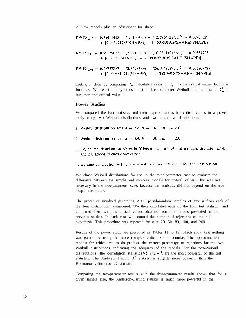
2. New models plus an adjustment for shape
Testing is done by comparing calculated using ln X( i) to the critical values from theformulas. We reject the hypothesis that a three-parameter Weibull fits the data if isless than the critical value.
Power Studies
We compared the four statistics and their approximations for critical values in a powerstudy using two Weibull distributions and two alternative distributions:
We chose Weibull distributions for use in the three-parameter case to evaluate thedifference between the simple and complex models for critical values. This was notnecessary in the two-parameter case, because the statistics did not depend on the trueshape parameter.
The procedure involved generating 2,000 pseudorandom samples of size n from each ofthe four distributions considered. We then calculated each of the four test statistics andcompared them with the critical values obtained from the models presented in theprevious section. In each case we counted the number of rejections of the nullhypothesis. This procedure was repeated for n = 20, 50, 80, 100, and 200.
Results of the power study are presented in Tables 11 to 13, which show that nothingwas gained by using the more complex critical value formulas. The approximationmodels for critical values do produce the correct percentage of rejections for the twoWeibull distributions, indicating the adequacy of the models. For the non-Weibulldistributions, the correlation statistics and are the most powerful of the teststatistics. The Anderson-Darling A2 statistic is slightly more powerful than theKolmogorov-Smirnov D statistic.
Comparing the two-parameter results with the three-parameter results shows that for agiven sample size, the Anderson-Darling statistic is much more powerful in the
10

Conclusions
References
two-parameter case than in the three-parameter case. Conversely, the correlation test ismore powerful in the three-parameter case than in the two-parameter case.
Four general conclusions are readily apparent from the results of this study:
1. Of the three statistics considered, the Anderson-Darling A2 statistic appears to bethe statistic of choice for testing the goodness-of-fit of a two-parameter Weibulldistribution to a set of data because of the larger power it displayed in the powerstudies. The choice might be different if censored data were used since thecorrelation statistic has the potential advantage of being easily modified for type Iand type II censored observations.
2. For testing the three-parameter Weibull goodness-of-fit, the correlation statisticsand appear to be the best because of their greater power against the alternativedistributions considered.
3. The critical value approximations appear to be very good for the range of samplesizes considered. For the two-parameter Weibull distribution critical values, this isseen in the close agreement of the plotted curves and the critical values as shown inFigures 1 to 3. For the three-parameter Weibull distribution critical values, thequality of the approximations can be seen in the power study where powers for theWeibull distributions tested were near the significance level of the test.
4. The power of the tests is very dependent upon the true distributional form of thedata. For example, in the two-parameter Weibull distribution power study, poweragainst the uniform distribution was much higher than against the truncated normal.
Bush, J.G.; Woodruff, B.W.; Moore, A.H.; Dunne, E.J. 1983. Modified Cramer-von Mises and Anderson-Darling tests for Weibull distributions with unknown locationand scale parameters. Communications in Statistics, Part A-Theory and Methods. 12:2465-2476.
Chandra, M.; Singpurwalla, N.D.; Stephens, M.A. 1981. Kolmogorov statistics fortests of fit for the extreme-value and Weibull distribution. Journal of the AmericanStatistics Association. 76: 729-731.
David, F.N.; Johnson, N.L. 1948. The probability integral transformation whenparameters are estimated from the sample. Biometrika. 35:182-190.
Filliben, J. 1975. The probability plot correlation coefficient test for normality.Technometrics. 17:111-117.
IMSL. 1979. Reference Manual. Houston, TX: International Mathematical andStatistical Libraries, Inc.
Lawless, J.F. 1982. Statistical Models and Methods for Lifetime Data. New York:John Wiley and Sons.
Lemon, G. 1975. Maximum likelihood estimation for the three-parameter Weibulldistribution, based on censored samples. Technometrics. 17:247-254.
11

Littell, R.D.; McClave, J.R.; Offen, W.W. 1979. Goodness-of-fit test for thetwo-parameter Weibull or extreme-value distribution with unknown parameters.Communications in Statistics, Part B-Simulation and Computation. 8: 257-269.
Mann, N.R.; Scheuer, E.M.; Fertig, K.W. 1973. A new goodness-of-fit test for the twoparameter Weibull or extreme-value distribution with unknown parameters.Communications in Statistics. 2:383-400.
Shapiro, S.S.; Francia, R.S. 1972. Approximate analysis of variance tests fornormality. Journal of the American Statistics Association. 67: 215-216.
Shapiro, S.S.; Wilk, M.B.; Chen, H. 1968. A comparative study of various tests fornormality. Journal of the American Statistics Association. 63: 1343-1372.
Smith, R.M.; Bain, L.J. 1976. Correlation type goodness-of-fit statistics with censoredsampling. Communications in Statistics, Part A-Theory and Methods. 5:119-132.
Stephens, M.A. 1977. Goodness-of-fit for the extreme value distribution. Biometrika.64: 583-588.
Tiku, M.L.; Singh, M. 1981. Testing the two parameter Weibull distribution.Communications in Statistics, Part A-Theory and Methods. 10:907-917.
Wilk, M.B.; Gnanadesikan, R. 1968. Probability plotting methods for the analysis ofdata. Biometrika. 55:1-19.
Woodruff, B.W.; Moore, A.H.; Dunne, E.J.; Cortes, R. 1983. A modifiedKolmogorov-Smirnov test for Weibull distributions with unknown location and scaleparameters. IEEE Transactions on Reliability. 2:209-212.
Wozniak, P.J.; Warren, W.G. 1984. Goodness of fit for the two-parameter Weibulldistribution. Presented at the American Statistical Association National Meeting,Philadelphia, PA.

Table 1 –Two-parameter Weibull critical values for the Kolmogorov-Smirnov D statistic based onmaximum likelihood estimates
Critical values at various significance levels
Samplesize 0.20
Littell and others (1979)a
0.15 0.10 0.05 0.01
Chandra and others (1981)
0.10 0.05 0.025 0.01
a Values multiplied by n1/2 to convert to the scale of Chandra and others (1981)b These are theoretical asymptotic values given by Chandra and others (1981).
Table 2–Two-parameter Weibull critical values for the Anderson-Darling A2 statistic based onmaximum likelihood estimates
Samplesize
Critical values at various significance levels
Wozniak and Warren (1984) Stephens (1977) Littell and others (1979)
0.10 0.05 0.01 0.10 0.05 0.01 0.10 0.05 0.01
a Theoretical asymptotic values.
13

Table 3–Two-parameter Weibull critical values for D, A2 , and
Samplesize
Critical values at various significance levels
Statistic 0.20 0.15 0.10 0.05 0.01
14

Table 3–Two-parameter Weibull critical values for D, A2 , and –con.
Samplesize Statistic
Critical values at various significance levels
0.20 0.15 0.10 0.05 0.01
Table 4–Simulated powers of two-parameter Weibull test statisticsa -αα = 0.10
Sample D A2
Distribution size T F T F T F
a Values from table (T) and formula (F).
15
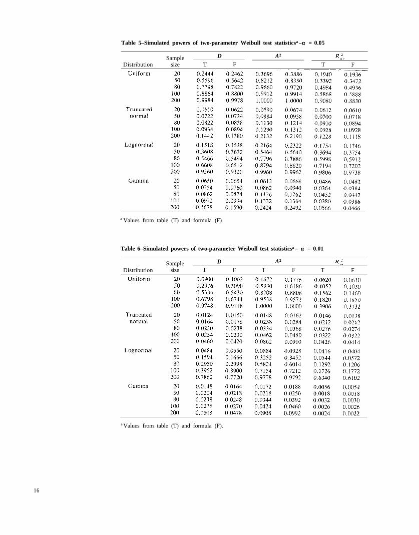
Table 5–Simulated powers of two-parameter Weibull test statisticsa –α α = 0.05
Sample D
Distribution size T F
A2
T F
a Values from table (T) and formula (F)
Table 6–Simulated powers of two-parameter Weibull test statisticsa – α α = 0.01
Sample D A2
Distribution size T F T F T F
a Values from table (T) and formula (F).
16
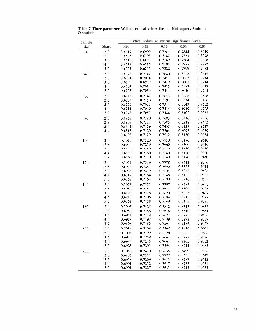
Table 7–Three-parameter Weibull critical values for the Kolmogorov-SmirnovD statistic
Samplesize Shape
Critical values at various significance levels
0.20 0.15 0.10 0.05 0.01
17

Table 8–Three-parameter Weibull critical values for the Anderson-DarlingA2 statistic
Samplesize Shape
Critical values at various significance levels
0.20 0.15 0.10 0.05 0.01
18

Table 9–Three-parameter Weibull critical values for the correlation teststatistic
Samplesize Shave
Critical values at various significance levels
0.20 0.15 0.10 0.05 0.01
19

Table 10–Three-parameter Weibull critical values for the correlation teststatistic
Samplesize Shape
Critical values at various significance levels
0.20 0.15 0.10 0.05 0.01
20
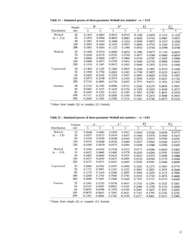
Table 11 – Simulated powers of three-parameter Weibull test statisticsa – α α = 0.10
Simple D A2
Distribution size S C S C S C S C
a Values from simple (S) or complex (C) formula.
Table 12 – Simulated powers of three-parameter Weibull test statisticsa – α α = 0.05
Simple D A 2
Distribution size S C S C S C S C
a Values from simple (S) or complex (C) formula
21

Table 13–Simulated powers of three-parameter Weibull test statisticsa – α α = 0.01
Simple D A2
Distribution size S C S C
a Values from simple (S) or complex (C) formula.
S C S C
22
Appendix –Some InvarianceProperties ofthe Statistics
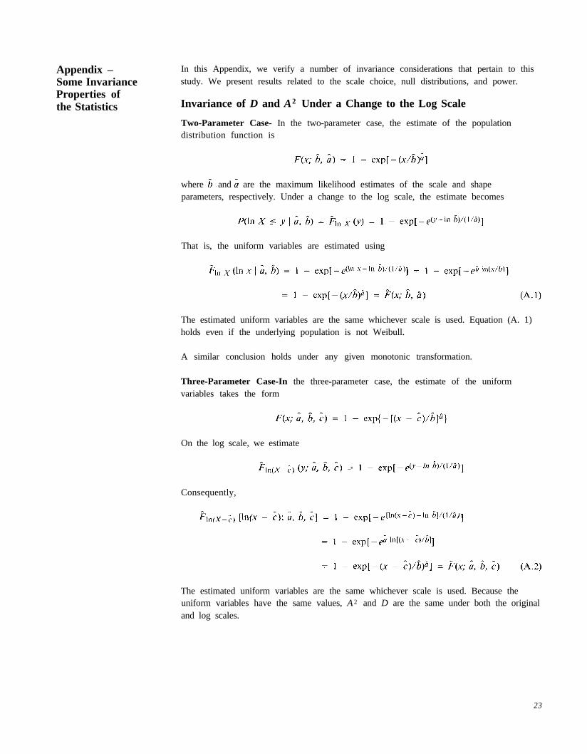
That is, the uniform variables are estimated using
The estimated uniform variables are the same whichever scale is used. Equation (A. 1)holds even if the underlying population is not Weibull.
A similar conclusion holds under any given monotonic transformation.
Three-Parameter Case-In the three-parameter case, the estimate of the uniformvariables takes the form
On the log scale, we estimate
Consequently,
In this Appendix, we verify a number of invariance considerations that pertain to thisstudy. We present results related to the scale choice, null distributions, and power.
Invariance of D and A2 Under a Change to the Log Scale
Two-Parameter Case- In the two-parameter case, the estimate of the populationdistribution function is
where and are the maximum likelihood estimates of the scale and shapeparameters, respectively. Under a change to the log scale, the estimate becomes
The estimated uniform variables are the same whichever scale is used. Because theuniform variables have the same values, A2 and D are the same under both the originaland log scales.
23

Appendix –Some InvarianceProperties ofthe Statistics
That is, the uniform variables are estimated using
The estimated uniform variables are the same whichever scale is used. Equation (A. 1)holds even if the underlying population is not Weibull.
A similar conclusion holds under any given monotonic transformation.
Three-Parameter Case-In the three-parameter case, the estimate of the uniformvariables takes the form
On the log scale, we estimate
Consequently,
In this Appendix, we verify a number of invariance considerations that pertain to thisstudy. We present results related to the scale choice, null distributions, and power.
Invariance of D and A2 Under a Change to the Log Scale
Two-Parameter Case- In the two-parameter case, the estimate of the populationdistribution function is
where and are the maximum likelihood estimates of the scale and shapeparameters, respectively. Under a change to the log scale, the estimate becomes
The estimated uniform variables are the same whichever scale is used. Because theuniform variables have the same values, A2 and D are the same under both the originaland log scales.
23
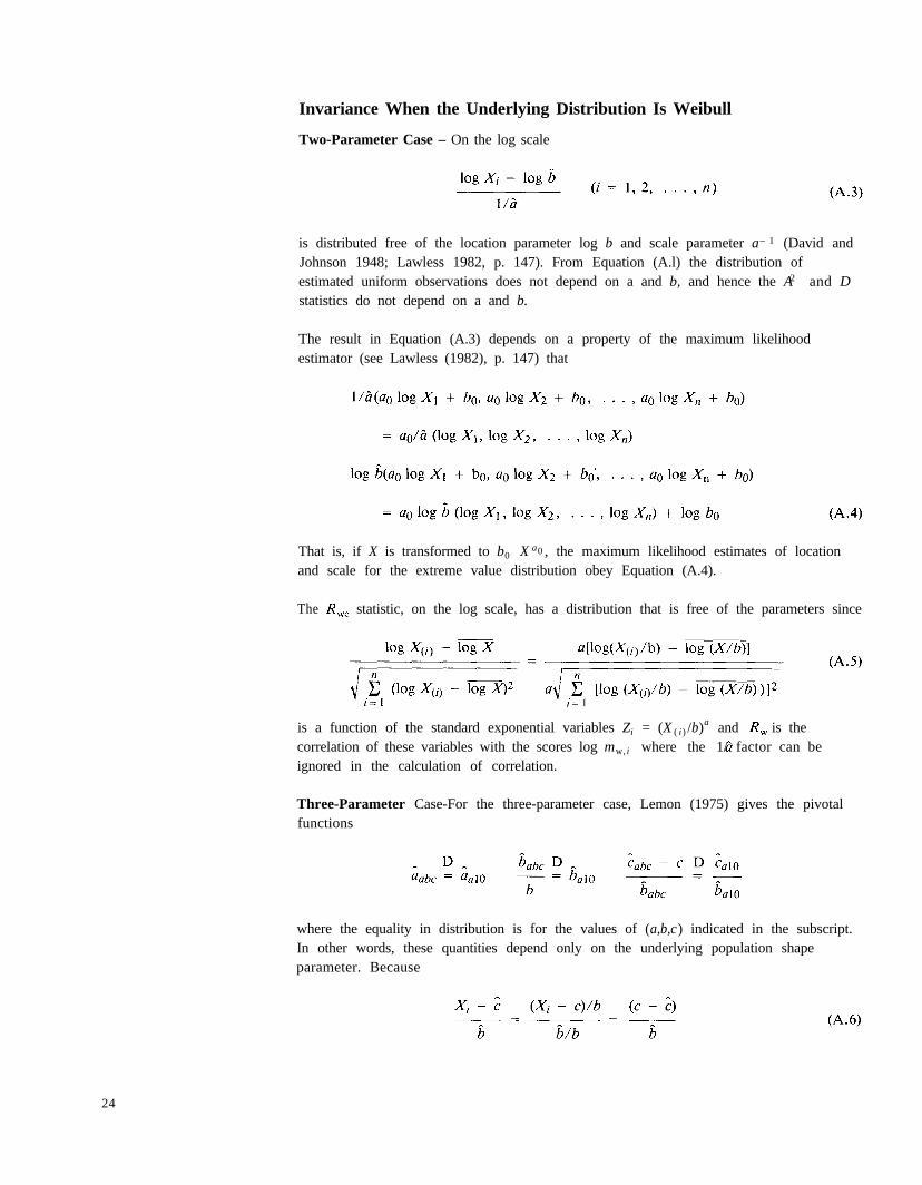
Invariance When the Underlying Distribution Is Weibull
Two-Parameter Case – On the log scale
is distributed free of the location parameter log b and scale parameter a– 1 (David andJohnson 1948; Lawless 1982, p. 147). From Equation (A.l) the distribution ofestimated uniform observations does not depend on a and b, and hence the A2 and Dstatistics do not depend on a and b.
The result in Equation (A.3) depends on a property of the maximum likelihoodestimator (see Lawless (1982), p. 147) that
That is, if X is transformed to b0 X a0 , the maximum likelihood estimates of locationand scale for the extreme value distribution obey Equation (A.4).
The statistic, on the log scale, has a distribution that is free of the parameters since
is a function of the standard exponential variables Zi = (X ( i) /b)a and is thecorrelation of these variables with the scores log mw, i where the 1/ factor can beignored in the calculation of correlation.
Three-Parameter Case-For the three-parameter case, Lemon (1975) gives the pivotalfunctions
where the equality in distribution is for the values of (a,b,c) indicated in the subscript.In other words, these quantities depend only on the underlying population shapeparameter. Because
24

where the distribution of each term depends only on a, the estimated uniform variablesin Equation (A.2) and hence the distributions of A2 and D depend only on a, not theother parameters.
In the case of the R w statistic, on the original scale,
which is a function of the standard Weibull with parameters a10. Since Rw is thecorrelation of these variables with the scores mw , i and the scores only depend on , andhence a, the distribution of Rw depends only on a.
For the log scale,
Similar to Equation (A.6),
has a distribution that depends only on a. Since Rw is the correlation of the variables(A.7) with the scores ln mw ,i , its distribution also depends only on a.
Invariance and Power
Because of the properties (Eq. (A.4)) of the maximum likelihood estimators, the powercalculations pertain to a wider class of alternatives than is immediately apparent.
Two-Parameter Case – Let X be distributed as GO(x) and let Y = b0 Xa 0 . Then log Yi =a,, log Xi + log b0. On the log scale, Rw e is a correlation and hence it has the samevalue whether calculated in terms of the log Yi or the log Xi.
Further,
by the properties in Equation (A.4). Consequently, the estimated uniform variables arethe same on both scales, so A2 and D do not depend on the scale.
Thus, the power of each of the three tests remains the same for any lognormaldistribution. Also, the powers for the uniform (0, 1) alternative hold for the uniform(0, > 0 and, more generally, for
25

The basic relations between the maximumbe shown directly. Let Y = Then
likelihood estimators on the two scales can
Consequently, the maximum likelihood estimates based on x and y (or equivalently onln y) satisfy
Because of this relation the estimated uniform variables are also equal.
Three-Parameter Case-Although there is a wider invariance class, we note that thepower for the three-parameter case is the same for any scale change. Let X bedistributed as G0 (x) and let Y = b0 X + c0. On the original scale, Rw, is a correlationand so its value is unchanged. The scores involving â are the same on both scales.More generally, the maximum likelihood estimates are related as follows:
Consequently, if maximize L(y | a, b, c), then
maximize L(x | a, b, c). In this sense, the maximum likelihood estimators andare equivariant.
26

According to Equation (A.9)
By Equation (A.2), the estimated uniform variables are equal, and we conclude thatpower is the same under both G0 (x) and any location scale change
27


