Download - Turbulence Measurements with Acoustic Doppler …laboratorios.fi.uba.ar/mincyt/docs/1288320366.pdf · S/2 Nyquist theorem, see Bendat and Piersol 2000 . This indicates that energy

Turbulence Measurements with AcousticDoppler Velocimeters

Carlos M. García1; Mariano I. Cantero2; Yarko Niño3; and Marcelo H. García4

Abstract: The capability of acoustic Doppler velocimeters to resolve flow turbulence is analyzed. Acoustic Doppler velocimeter perfor-mance curves �APCs� are introduced to define optimal flow and sampling conditions for measuring turbulence. To generate the APCs, aconceptual model is developed which simulates different flow conditions as well as the instrument operation. Different scenarios aresimulated using the conceptual model to generate synthetic time series of water velocity and the corresponding sampled signals. Mainturbulence statistics of the synthetically generated, sampled, and nonsampled time series are plotted in dimensionless form �APCs�. Therelative importance of the Doppler noise on the total measured energy is also evaluated for different noise energy levels and flowconditions. The proposed methodology can be used for the design of experimental measurements, as well as for the interpretation of bothfield and laboratory observations using acoustic Doppler velocimeters.

DOI: 10.1061/�ASCE�0733-9429�2005�131:12�1062�

CE Database subject headings: Flow measurement; Doppler systems; Turbulent flow; Filters; Noise.

Introduction

Present day laboratory and field research in fluid dynamics oftenrequires water velocity measurements with a high temporal andspatial resolution. Laser Doppler velocimetry �LDV� and particleimage velocimetry �PIV� have become the most common measur-ing techniques used in laboratory studies that satisfy such require-ments. However, the feasibility of using these techniques is re-duced when the scale of the experiment increases. The use ofPIV/LDV may also be unsuitable in flows with suspended sedi-ment concentrations. On the other hand, the use of hot wire an-emometers, which provides a very good temporal resolution, israther limited when impurities are present in the water, thus pre-cluding applications with sediment transport or where it becomesdifficult to control water quality that render the flow opaque. Inmost of these cases, acoustic Doppler velocimetry is the tech-

1Research Assistant, Ven Te Chow Hydrosystems Laboratory, Dept. ofCivil and Environmental Engineering, Univ. of Illinois at Urbana–Champaign, 205 North Mathews Ave., Urbana, IL 61801. E-mail:[email protected]

2Research Assistant, Ven Te Chow Hydrosystems Laboratory, Dept. ofCivil and Environmental Engineering, Univ. of Illinois at Urbana–Champaign, 205 North Mathews Ave., Urbana, IL 61801. E-mail:[email protected]

3Associate Professor, Dept. of Civil Engineering, Univ. of Chile,Casilla 228-3, Santiago, Chile. E-mail: [email protected]

4Chester and Helen Siess Professor, and Director, Ven Te ChowHydrosystems Laboratory, Dept. of Civil and EnvironmentalEngineering, Univ. of Illinois at Urbana–Champaign, 205 North MathewsAve., Urbana, IL 61801. E-mail: [email protected]

Note. Discussion open until May 1, 2006. Separate discussions mustbe submitted for individual papers. To extend the closing date by onemonth, a written request must be filed with the ASCE Managing Editor.The manuscript for this paper was submitted for review and possiblepublication on April 6, 2004; approved on March 23, 2005. This paper ispart of the Journal of Hydraulic Engineering, Vol. 131, No. 12,December 1, 2005. ©ASCE, ISSN 0733-9429/2005/12-1062–1073/
$25.00.
1062 / JOURNAL OF HYDRAULIC ENGINEERING © ASCE / DECEMBER 20

Downloaded 06 Jan 2009 to 130.126.32.13. Redistribution subject to

nique of choice, because it is relatively low in cost, can record ata relatively high frequency �up to 100 Hz�, and has a relativelysmall sampling volume �varies from 0.09 to 2 cm3 according tothe instrument selected�. Additionally, the measurements are per-formed in a remote control volume �located between 5 to 18 cmfrom the sensor according to the instrument selected�, which re-duces the interference with the flow being measured. ADV andNDV are trademark names for acoustic Doppler velocimetersmanufactured by Sontek and Nortek, respectively.

Acoustic Doppler velocimeters are capable of reporting accu-rate mean values of water velocity in three directions �Kraus et al.1994; Lohrmann et al. 1994; Anderson and Lohrmann 1995; Laneet al. 1998; Voulgaris and Trowbridge 1998; Lopez and García2001�, even in low flow velocities �Lohrmann et al. 1994�. How-ever, the ability of this instrument to accurately resolve flow tur-bulence is still uncertain �Barkdoll 2002�.

Lohrmann et al. �1994� argued that the acoustic Doppler ve-locimeters resolution is sufficient to capture a significant fractionof the turbulent kinetic energy �TKE� of the flow. However, theyidentified the Doppler noise as a problem that causes the TKE tobe biased toward a high value. Anderson and Lohrmann �1995�detected a flattening of the power spectrum of the velocity signaldue to this Doppler noise, this suggests that an operational noiseis eventually reached where the higher-frequency components ofthe signal cannot be resolved adequately.

Most research related to the capability of acoustic Dopplervelocimeters to resolve the flow turbulence �specifically TKE andspectra� has focused on definition of the noise level present in thesignal and how it can be removed �Lohrmann et al. 1994; Ander-son and Lohrmann 1995; Lane et al. 1998; Nikora and Goring1998; Voulgaris and Trowbridge 1998; Lemmin and Lhermitte1999; McLelland and Nicholas 2000�. However, little attentionhas been dedicated to evaluating the filtering effects of the sam-pling strategy �spatial and temporal averaging� on the turbulentparameters �moments, spectra, autocorrelation functions, etc.�.Only the paper by Voulgaris and Trowbridge �1998� discussessome issues related to the effect of spatial averaging on turbu-
lence measurements.
05

ASCE license or copyright; see http://pubs.asce.org/copyright

The capability of acoustic Doppler velocimeters to resolveflow turbulence is analyzed herein by means of a new tool,termed the acoustic Doppler velocimeter performance curves�APCs�. These curves can be used to define optimal flow andsampling conditions for turbulence measurements using this kindof velocimeters. The performance of these tools is validatedherein using experimental results. The APCs are used to define anew criterion for good resolution measurements of the flow tur-bulence. In cases where this criterion cannot be satisfied, thesecurves can be used to make appropriate corrections.

Another set of curves are also introduced to evaluate the rela-tive importance of the Doppler noise energy on the total measuredenergy. In cases where the noise is significant, the noise energylevel needs to be defined and corrections to the turbulence param-eters �e.g., TKE, length and time scales, and convective velocity�must be performed.

Principle of Operation of Acoustic DopplerVelocimeters

An acoustic Doppler velocimeter measures three-dimensionalflow velocities using the Doppler shift principle, and the instru-ment consists of a sound emitter, three sound receivers, and asignal conditioning electronic module. The sound emitter gener-ates an acoustic signal that is reflected back by sound-scatteringparticles present in the water, which are assumed to move at thewater’s velocity. The scattered sound signal is detected by thereceivers and used to compute the Doppler phase shift, fromwhich the flow velocity in the radial or beam directions is calcu-lated. A detailed description of the velocimeter operation can befound in McLelland and Nicholas �2000�. In the present paper, abrief description of the instrument characteristics is included tofacilitate presentation of a suitable conceptual model for the ob-jectives detailed above.

The acoustic Doppler velocimeter uses a dual pulse-pairscheme with different pulse repetition rates, �1 and �2, separatedby a dwell time �D �McLelland and Nicholas 2000�. The longerpair of pulses is used for higher precision velocity estimates,while the shorter pulse is used for ambiguity resolution, assumingthat the real velocity goes beyond the limit resolvable by thelonger time lag. These pulse repetition rates can be adjusted bychanging the velocity range of the measurement. Each pulse is asquare-shaped pulse train of an acoustic signal �the frequency canbe 5, 6, 10, or 16 MHz, depending on the instrument selected�.The phase shift is calculated from the auto- and cross correlationcomputed for each single pulse-pair using pulse-to-pulse coherentDoppler techniques �Lhermitte and Serafin 1984�. The radial ve-locities vi �i=1,2,3� are computed using the Doppler relation

vi =C

4�fADV�d�

dt�

i

�1�

where C=speed of the sound in water; fADV�sound signal fre-quency �10 MHz�; and d� /dt�i�phase shift rate computed forreceiver i. The radial or beam velocities are then computed se-quentially for each receiver and, thus the time it takes to completea three-dimensional velocity measurement is given by

T = 3��1 + �D + �2 + �D� �2�

This process is conducted with a frequency fS �equal to 1/T�,which is between 100 and 263 Hz depending on the velocity
range and the user-set frequency fR �see Table 1�. Then, the radial
JOURNAL


or beam velocities are converted to a local Cartesian coordinatesystem �ux ,uy ,uz� using a transformation matrix that is deter-mined empirically �through calibration� by the manufacturer �e.g.McLelland and Nicholas 2000�.

During the time it takes to make a three-dimensional velocitymeasurement, the flow may vary, however, these high-frequencyvariations are smoothed out in the process of signal acquisitionand, therefore, cannot be captured by the instrument. Each radialvelocity, vi, is the result of the acoustic echo reflected by thesound-scattering particles in the water during an overall time T /3,and this is hence an average value of the real flow velocity in thistime interval. Also, each of the final Cartesian velocity compo-nents is an average of the three radial velocity components �theproduct of the transformation matrix and the radial velocity�. Thedirect implication of these features is that the Cartesian flow ve-locity represents an averaged value, over an interval time T, of thereal flow velocity. In this sense T can be considered as the instru-ment response time, and the process of acquisition itself can beseen as an analog filter with a cut-off frequency, 1 /T �or fS�. Thetime averaging process is analogous to the spatial averaging ofthe recorded velocity vectors that occurs within the measurementvolume.

Two main conclusions can be drawn from the considerationsabove. First, energy in the signal with a frequency higher than fS

is filtered out �i.e., acquisition process acts as a low-pass filter�.Second, aliasing of the signal occurs since the velocity signal issampled at a frequency fS, and the highest frequency that can beresolved by the instrument is fS /2 �Nyquist theorem, see Bendatand Piersol �2000��. This indicates that energy in the frequencyrange of fS /2� f � fS is folded back into the range 0� f � fS /2,which may or may not be of importance depending on the flowcharacteristics. Flows with a large convective velocity, Uc, willhave a considerable portion of the energy in the range of wave-lengths: fS / �2Uc�� f /Uc� fS /Uc, while flows with a low convec-tive velocity will have no energy in this range and, therefore,aliasing will not be of relevance.

After the digital velocity signal is obtained �with frequencyfS�, the instrument performs an average of N values to produce adigital signal with frequency FR= fS /N, which is the acousticDoppler velocimeter’s user-set frequency with which velocitydata are recorded. This averaging process is a digital nonrecursivefilter �Hamming 1983; Bendat and Piersol 2000�, the conse-quences of which are analyzed next.

Implications of Digital Averaging of Velocity Signals

Let x be the signal sampled at fS and let y be the signal obtainedafter digital averaging �with frequency fR�. The interval betweensamples of signal x is �tx=1/ fS and between samples of signal y

Table 1. Frequencies Used by Acoustic Doppler Velocimeter

Velocity range�cm/s�

fR �Hz� 1 25 100

fcut-off �Hz� 0.44 11.3 50

fS �Hz�

250 263 250 200

100 256 225 200

30 226 200 100

10 180 175 100

3 143 125 100

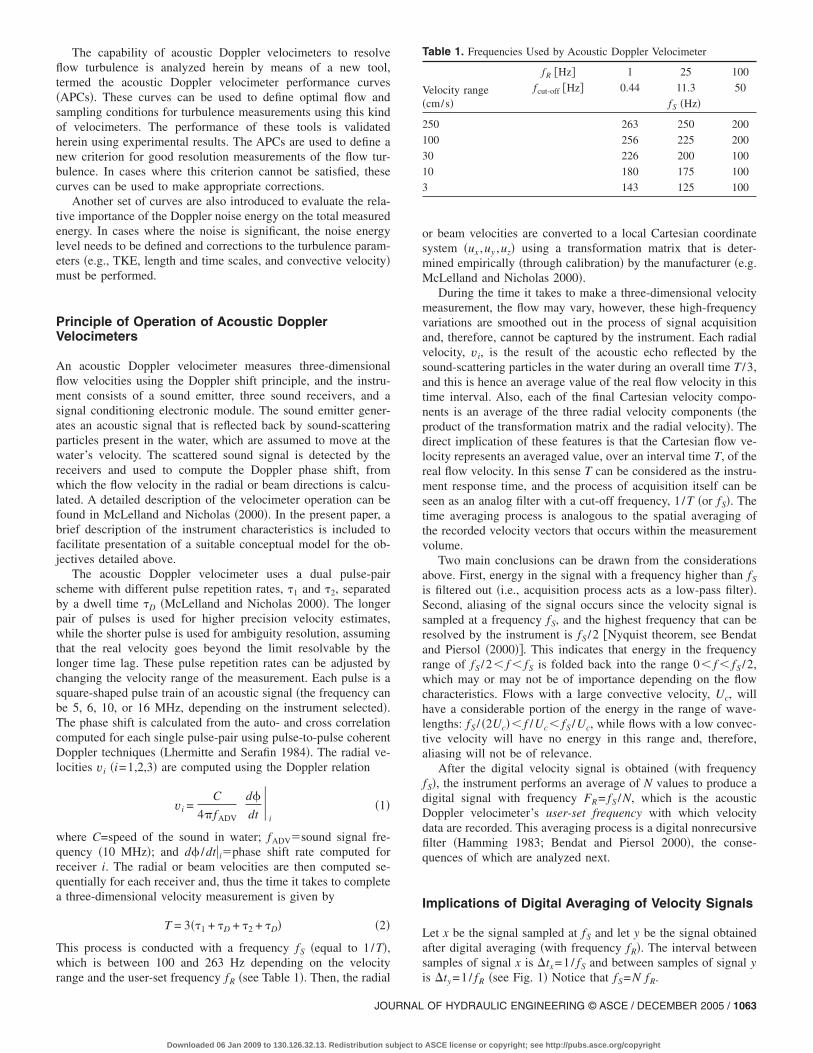
is �ty =1/ fR �see Fig. 1� Notice that fS=N fR.

OF HYDRAULIC ENGINEERING © ASCE / DECEMBER 2005 / 1063


The nonrecursive digital filter is given by

yi = �n=0

N−11

NxNi+n �3�

or in the time domain

y�t� = �n=0

N−11

Nx�t +

n

N fR �4�

where t= i �ty =N i �tx. The transfer function of this filter, H�f�,can be calculated by computing the Fourier transform of Eq. �4�,i.e.

H�f� =Y�f�X�f�

= �n=0

N−1 exp� j2�nf

N fR

N�5�

where Y�f� and X�f�=Fourier transforms; and j= �−1�1/2. The sumin Eq. �5� can be computed to give

H�f� =fR

fS

exp� j2�f

fR − 1

exp� j2�f

fS − 1

�6�

noting that NfR= fS. The gain factor of the filter is

�H�f�� =fR

fS1 − cos�2�

f

fR

1 − cos�2�f

fS �7�

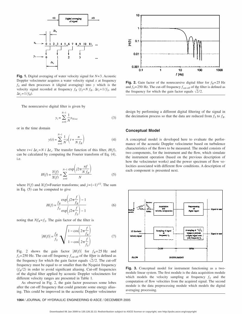
Fig. 2 shows the gain factor �H�f�� for fR=25 Hz andfS=250 Hz. The cut-off frequency fcut-off of the filter is defined asthe frequency for which the gain factor equals 2/2. The cut-offfrequency must be equal to or smaller than the Nyquist frequency�fR /2� in order to avoid significant aliasing. Cut-off frequenciesof the digital filter applied by acoustic Doppler velocimeters fordifferent velocity ranges are presented in Table 1.

As observed in Fig. 2, the gain factor possesses some lobesafter the cut-off frequency that could generate some energy alias-

Fig. 1. Digital averaging of water velocity signal for N=3. AcousticDoppler velocimeter acquires a water velocity signal x at frequencyfS and then processes it �digital averaging� into y which is thevelocity signal recorded at frequency fR �fS=N fR , �tx=1/ fS, and�ty =1/ fR�.

ing. This could be improved in the acoustic Doppler velocimeter



design by performing a different digital filtering of the signal inthe decimation process so that the data are reduced from fS to fR.

Conceptual Model

A conceptual model is developed here to evaluate the perfor-mance of the acoustic Doppler velocimeter based on turbulencecharacteristics of the flows to be measured. The model consists oftwo components, for the instrument and the flow, which simulatethe instrument operation �based on the previous description ofhow the velocimeter works� and the power spectrum of flow ve-locities associated with different flow conditions. A description ofeach component is presented next.

Fig. 2. Gain factor of the nonrecursive digital filter for fR=25 Hzand fS=250 Hz. The cut-off frequency fcut-off of the filter is defined asthe frequency for which the gain factor equals 2/2.

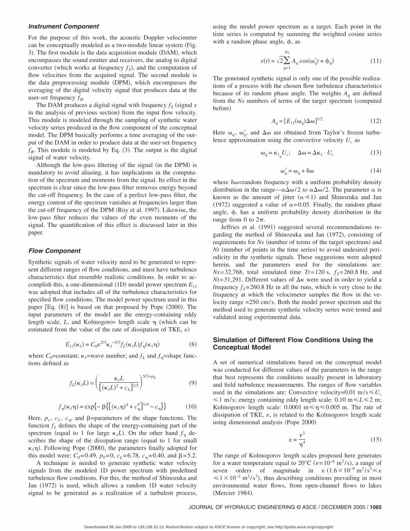
Fig. 3. Conceptual model for instrument functioning as a two-module linear system. The first module is the data acquisition modulewhich models the velocity sampling at frequency fS and thecomputation of flow velocities from the acquired signal. The secondmodule is the data preprocessing module which models the digitalaveraging processing.

05


Instrument Component

For the purpose of this work, the acoustic Doppler velocimetercan be conceptually modeled as a two-module linear system �Fig.3�. The first module is the data acquisition module �DAM�, whichencompasses the sound emitter and receivers, the analog to digitalconverter �which works at frequency fS�, and the computation offlow velocities from the acquired signal. The second module isthe data preprocessing module �DPM�, which encompasses theaveraging of the digital velocity signal that produces data at theuser-set frequency fR.

The DAM produces a digital signal with frequency fS �signal xin the analysis of previous section� from the input flow velocity.This module is modeled through the sampling of synthetic watervelocity series produced in the flow component of the conceptualmodel. The DPM basically performs a time averaging of the out-put of the DAM in order to produce data at the user-set frequencyfR. This module is modeled by Eq. �3�. The output is the digitalsignal of water velocity.

Although the low-pass filtering of the signal �in the DPM� ismandatory to avoid aliasing, it has implications in the computa-tion of the spectrum and moments from the signal. Its effect in thespectrum is clear since the low-pass filter removes energy beyondthe cut-off frequency. In the case of a perfect low-pass filter, theenergy content of the spectrum vanishes at frequencies larger thanthe cut-off frequency of the DPM �Roy et al. 1997�. Likewise, thelow-pass filter reduces the values of the even moments of thesignal. The quantification of this effect is discussed later in thispaper.

Flow Component

Synthetic signals of water velocity need to be generated to repre-sent different ranges of flow conditions, and must have turbulencecharacteristics that resemble realistic conditions. In order to ac-complish this, a one-dimensional �1D� model power spectrum E11

was adopted that includes all of the turbulence characteristics forspecified flow conditions. The model power spectrum used in thispaper �Eq. �8�� is based on that proposed by Pope �2000�. Theinput parameters of the model are the energy-containing eddylength scale, L, and Kolmogorov length scale � �which can beestimated from the value of the rate of dissipation of TKE, ��

E11�1� = C0�2/31−5/3fL�1L�f��1�� 8�

where C0=constant; 1=wave number; and fL and f�=shape func-tions defined as

fL�1L� = � 1L

��1L�2 + cL�1/25/3+p0

�9�

f��1�� = exp�− ��1��4 + c�4�1/4 − c�� 10�

Here, po , cL , c�, and =parameters of the shape functions. Thefunction fL defines the shape of the energy-containing part of thespectrum �equal to 1 for large 1L�. On the other hand f� de-scribes the shape of the dissipation range �equal to 1 for small1��. Following Pope �2000�, the parameters finally adopted forthis model were: C0=0.49, p0=0, cL=6.78, c�=0.40, and =5.2.

A technique is needed to generate synthetic water velocitysignals from the modeled 1D power spectrum with predefinedturbulence flow conditions. For this, the method of Shinozuka andJan �1972� is used, which allows a random 1D water velocity
signal to be generated as a realization of a turbulent process,
JOURNAL


using the model power spectrum as a target. Each point in thetime series is computed by summing the weighted cosine serieswith a random phase angle, �, as

x�t� = 2�q=1

Ns

Aq cos��q�t + �q� �11�

The generated synthetic signal is only one of the possible realiza-tions of a process with the chosen flow turbulence characteristicsbecause of its random phase angle. The weights Aq are definedfrom the Ns numbers of terms of the target spectrum �computedbefore�

Aq = �E11��q��1/2 �12�

Here �q , �q�, and �� are obtained from Taylor’s frozen turbu-lence approximation using the convective velocity Uc as

�q = 1qUc; �� = �1 · Uc �13�

�q� = �q + �� 14�

where ��=random frequency with a uniform probability densitydistribution in the range— �� /2 to �� /2. The parameter isknown as the amount of jitter � �1� and Shinozuka and Jan�1972� suggested a value of =0.05. Finally, the random phaseangle, �, has a uniform probability density distribution in therange from 0 to 2�.

Jeffries et al. �1991� suggested several recommendations re-garding the method of Shinozuka and Jan �1972�, consisting ofrequirements for Ns �number of terms of the target spectrum� andNt �number of points in the time series� to avoid undesired peri-odicity in the synthetic signals. These suggestions were adoptedherein, and the parameters used for the simulations are:Ns=32,768, total simulated time Tt=120 s, fS=260.8 Hz, andNt=31,291. Different values of � were used in order to yield afrequency fS=260.8 Hz in all the runs, which is very close to thefrequency at which the velocimeter samples the flow in the ve-locity range =250 cm/s. Both the model power spectrum and themethod used to generate synthetic velocity series were tested andvalidated using experimental data.

Simulation of Different Flow Conditions Using theConceptual Model

A set of numerical simulations based on the conceptual modelwas conducted for different values of the parameters in the rangethat best represents the conditions usually present in laboratoryand field turbulence measurements. The ranges of flow variablesused in the simulations are: Convective velocity=0.01 m/s�Uc

�1 m/s; energy containing eddy length scale: 0.10 m�L�2 m;Kolmogorov length scale: 0.0001 m��0.005 m. The rate ofdissipation of TKE, �, is related to the Kolmogorov length scaleusing dimensional analysis �Pope 2000�

� =�3

�4 �15�

The range of Kolmogorov length scales proposed here generatesfor a water temperature equal to 20°C ��=10−6 m2/s�, a range ofseven orders of magnitude in � �1.6�10−9 m2/s3��1�10−2 m2/s3�, thus describing conditions prevailing in mostenvironmental water flows, from open-channel flows to lakes
�Mercier 1984�.


Acoustic Doppler Velocimeter Performance CurvesSampling the Flow Turbulence

First, a set of 1D model spectra were computed for different flowconditions. These spectra were then integrated to compute flowenergies and evaluate both the effects of the analog filter withcut-off frequency fS, and the level of aliased energy with frequen-cies in the range fS /2� f � fS in the original �unsampled� timeseries. Such energy is folded back through the sampling processand confused with resolved energy corresponding to frequenciesin the range 0� f � fS /2.

The results obtained are shown in Fig. 4 in dimensionlessform. As the dimensionless number fS L /Uc increases, a smallerportion of the energy is both filtered and aliased. The poorestmeasurement conditions for the acoustic Doppler velocimeter inthe range of parameters considered, are defined by extreme flowconditions �L=0.1 m and Uc=1 m/s, which combined yield aminimum value of fS L /Uc at a given frequency� and the smallervelocimeter velocity range which can sample this convective ve-locity �equivalent to 1 m/s�. For this velocity range, atfR=25 Hz, the frequency fS�225 Hz �see Table 1�, and thus thevalue of the dimensionless number fS L /Uc is 22.5. In such acase, the analog filter would take about 8.4% of the total energyout of the signal when it is sampled at fS=225 Hz. Additionally,for frequencies equal to fS /2, the accumulated energy would be86.4% of the total energy in the flow, which implies that only5.2% of the total energy will be aliased. The values cited beforecorrespond to extreme conditions, and for lower values of Uc

�corresponding to a lower velocity range� and, consequently, forlower values of fS �see Table 1�, the percentage of aliased energyshould decrease. Based on the values cited before, it is concludedfrom the model behavior of the velocimeter that both the effectsof the analog filter �with cut-off frequency fS� and the level ofaliased energy are lower than 10% even in the most critical con-ditions. Besides, the digital filtering performed by the DPM usinga cut-off frequency smaller than fS /2 takes most of the aliasedenergy out of the spectrum.

Next, a number of synthetic turbulent water velocity signalswith �t=0.0038 s �fS=260.8 Hz� were generated as realizationsof different flow conditions and then sampled according to thesampling strategy described in the instrument component of theconceptual model. The use of different values of fS corresponding

Fig. 4. Percentage of the energy remaining in the sampled signal for:Curve A: f � fS; Curve B: f � fS /2; and Curve C=energycorresponding to frequencies fS /2� f � fS

to different velocity ranges does not affect the results of the



analysis performed herein, because the gain factor of the veloci-meter digital filtering does not depend on the number of averagedvalues in the signal to produce the same user-defined frequencyfR. The user-set frequencies adopted here were fR=260.8, 52.2,26.1, 10, 5, and 3 Hz. The sampled signals were analyzed in orderto compute corresponding turbulent parameters �up to fourth-order moments, autocorrelation function, power spectrum, andtime scales�. Thus, the variation of these parameters can be evalu-ated as flow conditions and sampling frequency change.

The effect of different flow conditions on the flow statistics isexplored in Figs. 5–8. The parameters representing the flowstatistics obtained for values fR� fS are made dimensionlessusing the corresponding value of the parameter computed forfR= fS=260.8 Hz �no averaging�. Those dimensionless parametersare plotted as a function of the dimensionless parameter F definedas

Fig. 5. Effects of digital averaging on second- and fourth-ordermoments of the water velocity signals. For F= fRL /Uc=20, thesecond- and fourth-order moments of the signal sampled at frequencyfR are about 90 and 80%, respectively, of the values of the parametersof the signal sampled at frequency fS.

Fig. 6. Autocorrelation function values at Lag 1 of the recordedwater velocity signal. Smaller values of Rxx�1� mean that there is lessturbulence sampled in these signals. For F= fRL /Uc=20, Rxx�1� is0.85.

05


F =L

Uc

fR

=fR

fT=

L

dR�16�

where fT=characteristic frequency of large eddies present in theflow; and dR=diameter of the sampled volume set by the flow andsampling characteristics. The higher the ratio F, the better thedescription of the turbulence that can be achieved with a specificinstrument. In theory, no turbulence scale could be described fromthe recorded signal for F�1.

So far, the sampling volume has been considered as a point.However, spatial averaging performed by acoustic Doppler ve-locimeters of the turbulence fluctuations in the longitudinal flowdirection of a uniform flow should be considered when the valueof dR is smaller than the diameter of the measurement volume, d.For instance, in the case of the 10 MHz Nortek velocimeter�d=6 mm, and fR=25 Hz�, dR�d for convective velocitiessmaller than 15 cm/s. In those cases, d must be used in Eq. �16�instead of dR because spatial averaging of the turbulence fluctua-tions becomes more important than the temporal averaging of theturbulence fluctuations. This replacement is based on the assump-tion that the spatial average of the turbulence fluctuations acts asa low-pass filter with wavelength =1/d. A similar analysis could

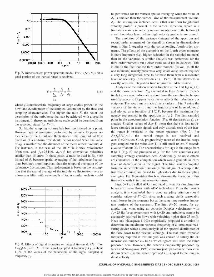
Fig. 7. Dimensionless power spectrum model. For F= fRL /Uc=20, agood portion of the inertial range is resolved.

Fig. 8. Effects of digital averaging on integral time scale �T11�. ForF= fRL /Uc=20, T11 of the signal sampled at frequency FR is about110% of the values of the parameters of the signal sampled atfrequency fS.

JOURNAL


be performed for the vertical spatial averaging when the value ofdR is smaller than the vertical size of the measurement volume,dv. The assumption included here is that a uniform longitudinalvelocity profile is present in the vertical direction, which is alimitation mainly in velocity measurements close to the bottom ofa wall boundary layer, where high velocity gradients are present.

The evolution of the variance �integral of the spectrum andsecond-order moment of the signal� is shown in dimensionlessform in Fig. 5, together with the corresponding fourth-order mo-ments. The effects of the averaging on the fourth-order momentsis more important �i.e., higher reduction in the sampled moment�than on the variance. A similar analysis was performed for thethird-order moments but a clear trend could not be detected. Thisis due to the fact that the third-order moment �as well as all theodd moments� usually presents a very small value, which requiresa very long integration time to estimate them with a reasonablelevel of accuracy �Sreenivasan et al. 1978�. If the skewness isexactly zero, the integration time required is indeterminate.

Analysis of the autocorrelation function at the first lag Rxx�1�,and the power spectrum E11 �included in Figs. 6 and 7, respec-tively� gives good information about how the sampling techniqueused by acoustic Doppler velocimeter affects the turbulence de-scription. The spectrum is made dimensionless in Fig. 7 using thevariance of the signal, �, and the length scale of large eddies, Land plotted as a function of 1 /2 F, because the maximum fre-quency represented in the spectrum is fR /2. The first sampledpoint in the autocorrelation function �Fig. 6� decreases as fR de-creases. Smaller values of Rxx�1� mean that there is less turbu-lence sampled in these signals and only a small zone of the iner-tial range is resolved in the power spectrum �Fig. 7�. ForF= fRL /Uc�1, the inertial range is not resolved andRxx�1�=20%. As F�2, progressively more of the inertial rangegets sampled but the value Rxx�1� is still small unless F exceedsa value of about 20. The decorrelations for lags in the range from0 to 1 �Fig. 6� are produced only for the flow conditions andsampling strategy considered here. Additionally, no noise effectsare considered in the computation which would generate an extralevel of decorrelation in the signal. The time scales computedfrom the autocorrelation function �as the integral of Rxx up to thefirst zero crossing� are biased to high values due to the samplingaveraging. Fig. 8 quantifies this bias, showing the variation of thistime scale with F in dimensionless terms.

Figs. 5–8 are called APCs, and yield criteria for sampling tur-bulence in water flows with ADV technology. From the presentanalysis, it is concluded that a good sampling criterion shouldconsider values of F�20, since such a range yields reasonablysmall losses in the moments but at the same time resolves impor-tant portions of the spectrum. The limit F=20 means, for ex-ample, that when using an acoustic Doppler velocimeter withfR=25 Hz for an experiment with L=20 cm, turbulence cannot beaccurately resolved in flows with velocities higher than 25 cm/s.Nezu and Nakagawa �1993� empirically proposed a criterion todetermine the maximum response frequency of a turbulence mea-suring device which allows analysis of the spectral distribution ofthe flow down to the viscous subrange. The maximum responsefrequency required in this analysis was chosen to satisfy the di-mensionless number F=16.67 which agrees well with the valueproposed here. However, the criterion empirically proposed byNezu and Nakagawa �1993� concerns just open-channel flow con-ditions where L is the water depth and Uc is equal to the longitu-
dinal velocity.


Validation of the Acoustic Doppler VelocimeterPerformance Curves

The assumptions used to develop the conceptual model are nowvalidated using experimental data from an open-channel flow, re-corded in a flume having a width B=0.91 m at the Ven Te ChowHydrosystems Laboratory, University of Illinois at Urbana–Champaign �UIUC�. First, a set of 11 three-dimensional watervelocity time series were obtained with a down-looking SontekMicro ADV �sampling volume 5 cm away from the probe� at thesame location, flow conditions and instrument velocity range, butwith different sampling frequencies �values of fR=50; 30; 25; 20;10; 5; 2; 1; 0.5; 0.2; 0.1 Hz�. The longitudinal water velocitysignals recorded for each configuration were used to developFigs. 9–12. The quality of the recorded signals is characterized bya correlation value in the range from 82 to 93 and a signal tonoise ratio �SNR� value in the range 17.9 to 22.9 dB, which arehigh enough values of these parameters to ensure good qualitydata. Water velocity signals were recorded for 2 min at each in-strument configuration. The sampling volume of the velocimeterwas located at yp=0.04 m from the bottom of the flume. The flowcondition analyzed consisted of a water depth h=0.282 m, flowdischarge Q=0.12 �m3/s�, and a local value of the shear velocityat this vertical, u*=0.0482 m/s. The scale of the energy contain-ing eddies, L, corresponding to this flow is estimated to be equal

Fig. 9. Comparison between observed and predicted digitalaveraging effect on the variance of the recorded water velocity signal

Fig. 10. Comparison between observed and predicted digitalaveraging effect on the fourth-order moment of the recorded watervelocity signal



to the depth=0.282 m, and the associated convective velocityis determined to be equal to Uc=0.58 m/s, from the three-dimensional velocity vector data using the relation proposed byHeskestad �1965�

Uc12 = U1

2 1 + 2U2

2

U12 + 2

U32

U12 +

u1�2

U12 + 2

u2�2

U12 + 2

u3�2

U12 � �17�

where Ui and ui�=mean and the fluctuation of the flow velocity inthe i Cartesian direction. Following Nezu and Nakagawa �1993�,the dimensionless parameter �h /u*3 is estimated to have a valueequal to 16 for yp /h=0.142. Thus, the rate of dissipation of TKEat the measurement point is 6.35�10−3 m2/s3 and the corre-sponding Kolmogorov length scale is 0.00011 m.

The evolution of second- and fourth-order moments of themeasured velocity signals as fR varies is plotted in Figs. 9 and 10,respectively. The values of the moments corresponding to the realsampling frequency, fS, of the instrument are needed to make theplot dimensionless; however, this information cannot be obtainedfrom the acoustic Doppler velocimeters. To overcome this prob-lem, the value of the ratio between the corresponding momentsobtained at fR and fS for the higher sampling frequency�fR=50 Hz and F=24.31� is assumed to be the same as that pre-dicted by the conceptual model �92.5% for the variance and 83%

Fig. 11. Comparison between observed and predicted autocorrelationfunction value at Lag 1 of the recorded water velocity signal

Fig. 12. Comparison between observed and predicted digitalaveraging effect on integral time scale �T11� of the recorded watervelocity signal

05


for the fourth-order moment�. The trend obtained from the mea-surements agrees very well with that predicted by the model�Figs. 9 and 10�. The poor resolution of turbulence in the ana-lyzed flow obtained with low sampling frequencies is shown bythese figures by the fact that all of the even moments of thesampled frequencies are biased to low values. For instance, atfrequency fR=1 Hz �F= fRL /Uc=0.4862�, the recorded signalcaptured only 48.5 and 24% of the variance and fourth-order mo-ment, respectively.

A good agreement is also obtained between measurements andthe predictions of the conceptual model for the variation of thecorrelation value at the first lag, Rxx�1� with the dimensionlessfrequency F �Fig. 11�. The observed values of Rxx�1� reach arather constant value of about 80% at high frequencies due to thenoise decorrelation. Fig. 12 shows the observed variation of theintegral time scale with F. A good agreement is obtained betweenthe prediction of the conceptual model and the observations, withexception of the behavior at dimensionless frequencies lower thanabout unity.

Further validation of the conceptual model was obtained byusing water velocity signals recorded at several facilities by re-searchers at the Ven Te Chow Hydrosystems Laboratory of theUIUC since 1994. Corresponding experimental conditions are de-scribed in Table 2. The flow generated in an annular flume wasanalyzed in Experiment 1; open-channel flow conditions weresimulated in three different tilting flumes for Experiments 2–5; inExperiment 6, water velocities signals were recorded in an experi-mental pool and riffle sequence with and without the presence ofvegetation, respectively; flow velocity fields around bubbleplumes were measured in Experiments 8 and 9 in a square andround tank, respectively; and finally, flow velocity signals re-corded at points located inside a turbidity current were analyzedin Experiment 10. Experiment 7 is the source of data for the set of11 time series used in Figs. 9–12. For the sake of clarity, only twopoints of this set are used in Fig. 13. These time series correspondto values of F=12.02 and F=24.3. The data included in Fig. 13correspond only to velocity signals of the X Cartesian componentfrom all of the experiments. This component was always alignedwith the main flow direction. In all cases, the instrument was usedin a down-looking orientation, with the exception of Experiments3, 8, and 9, where a side-looking orientation was used. In sum-mary, the quality of the recorded signals is characterized by cor-relation values in the range 84 to 99 and by SNR values in therange 18.6 to 30.20 DB.

Table 2. Characteristics of the Experiments

Experimentno.

Flowconditions Instrument

L�cm�

Uc

�cm/s� TypefR

�Hz�

1 20 �43 Micro ADV Sontek 10

2 38 5–7 Micro ADV Sontek 25

3 50–60 15–23 Nortek NDV 10 MHz 25

4 85 17–22 ADV Sontek 25

5 365.8 �10 Nortek NDV 10 MHz 25

6 26.7 56–71 Micro ADV Sontek 25

7 28.2 58 Micro ADV Sontek 25

8 80 5–9 Micro ADV Sontek 25

9 700 12–13 Nortek NDV 10 MHz 10

10 15 10–21 ADV Sontek 25

Comparisons between the predicted and observed values of the

JOURNAL


autocorrelation function at Lag 1 for experimental conditions de-scribed in Table 2 are presented in Fig. 13. The decorrelationobserved in the measured signals increases as the dimensionlessnumber F decreases, in agreement with the predictions of theconceptual model. However, decorrelations that are higher thanthose predicted are observed due to noise effects, which are notaccounted for by the theoretical APC curves. Based on this ob-servation, it can be argued that these curves provide an upperlimit of the actual ones.

Noise Effects from Turbulence ParametersComputed from Acoustic Doppler VelocimeterWater Velocity Signals

The presence of noise in water velocity signals obtained using anacoustic Doppler velocimeter, and the techniques to reduce itseffect in the computation of turbulence parameters obtained fromthese signals, have been the focus of several papers in recentyears �Lohrmann et al. 1994; Nikora and Goring 1998; Voulgarisand Trowbridge 1998; McLelland and Nicholas 2000�. Evenwhen all of the possible precautions suggested by the manufac-turers are taken into consideration �i.e., correlation, �, and SNRwithin defined ranges�, the signal will have a noise level thataffects the values of the turbulence parameters. Nikora and Gor-ing �1998� and SonTek �1997� affirm that the main physical con-tributor to the acoustic Doppler velocimeter’s noise is the Dopplernoise. The Doppler noise has the characteristics of white noise�Nikora and Goring 1998; Lemmin and Lhermitte 1999; McLel-land and Nicholas 2000� with a Gaussian probability distribution�Nikora and Goring 1998�, as well as a flat power spectrum�Anderson and Lohrmann 1995� which indicates the presence ofuncorrelated noise �Lemmin and Lhermitte 1999�.

The fact that white noise presents the same energy level for allfrequencies makes it impossible to subtract its effects from thetemporal series using digital filters: however, its integral effectscan be subtracted from some turbulence parameters. White noisedoes not affect the computation of the mean values because it haszero mean. Nikora and Goring �1998�, Voulgaris and Trowbridge�1998�, and McLelland and Nicholas �2000� showed that Rey-nolds stress computations are not affected by the presence of thewhite noise. Lohrmann et al. �1994� considered that the Reynolds

Fig. 13. Comparison between observed and predicted autocorrelationfunction value at Lag 1 of the recorded water velocity signals fordifferent experimental conditions �see Table 2�

stresses can be accurately determined even at levels below the



Doppler noise. Nikora and Goring �1998� claim that estimates ofTKE are limited by the Doppler noise because the TKE is biasedto high values. However, Lohrmann et al. �1994�, Nikora andGoring �1998�, and Gordon and Cox �2000� affirm that the con-tributions of noise over the total energy can be considered negli-gible for flows with high levels of turbulence, such as open-channel flow boundary layers.

The Doppler noise produces decorrelation of the signal andhence the autocorrelation function reduces its value to zero fasterthan in signals without noise. Consequently, the temporal scalesobtained from this function are biased to low values. On the otherhand, velocity spectra for the horizontal velocity components arebiased toward high values due to the presence of the Dopplernoise, while for the vertical velocity the noise is negligible �Lo-hrmann et al. 1994; Nikora and Goring 1998�. Assuming that thenoise and turbulent fluctuations are decorrelated �Nikora and Gor-ing 1998�, the spectrum of the resulting measurement is the sumof the turbulent spectrum plus the noise level. Nikora and Goring�1998� identified the Doppler noise as a flattening of the spectrumclose to the Nyquist frequency, and found that in the worst casethe flattening may take place around 4–5 Hz for the horizontalvelocity but is more typically in the range of 5–10 Hz.

The main parameter used to subtract the Doppler noise effectson the turbulence parameters is the white noise energy level, thedetection of which is discussed later. Using this level, the cor-rected power spectrum for each velocity component can be sim-ply obtained by subtracting the white noise energy level from themeasured spectra. Thus, by integrating the corrected power spec-tra, the corrected variances for each component, and from thesethe corrected TKE are computed. Additionally, the inverse fastFourier transform of the corrected power spectrum can be used toestimate the autocorrelation function and associated correctedtime scales can be obtained.

Detection of the Doppler Noise Energy Level

In a low-energy flow, the energy level of the white noise can beidentified in a power spectrum as a flat plateau at high frequen-cies. Nikora and Goring �1998� suggested that the empirical spec-tra of the Doppler noise can be replaced by straight horizontallines whose ordinates are equal to the average of the noise spec-tral ordinates. This technique was called “spectral analysis” byVoulgaris and Trowbridge �1998�, who calculated the noise en-ergy using the noise energy level detected in the tail of the spec-trum �the frequency range is chosen so that there are ten estimatesfor the calculation of the statistically significant average, i.e.,11.5–12.5 Hz for sampling frequency=25 Hz�.

Nikora and Goring �1998� identified a characteristic frequency,fn, that demarks a boundary in the power spectrum between tworegions. The first region corresponds to frequencies smaller thanfn, where the turbulence energy is much larger than the noiseenergy. In the other region, for frequencies higher than fn, turbu-lence energy is weaker than the noise energy. If the frequency fn

is smaller than the Nyquist frequency �fR /2�, the flat plateau inthe spectrum would be visualized. In these cases, the spectralanalysis technique of Voulgaris and Trowbridge �1998� can beapplied to estimate the noise energy level. Although this methodbecomes a very good approximation to determine the noise en-ergy level, for high-energy flows the plateau cannot be distin-guished in the spectrum, although this does not imply that thesignal does not have intrinsic noise. In these cases, different meth-
odologies have been suggested to estimate the noise level �Nikora


and Goring 1998; Voulgaris and Trowbridge 1998; McLellandand Nicholas 2000�, which all have some intrinsic difficulties.These methods mainly assume that the noise level of the signal isthe same if the instrument configuration and flow conditions donot change. This implies that the users are recording signals withthe same quality each time that the instrument is sampling thesame flow conditions with the same configuration �sampling fre-quency, velocity range, etc.�. However, there are certain condi-tions that cannot be controlled by the users during the measure-ment �for example, level of seeding particles, and bubblesattached to the sensor� which strongly affect the quality of thesignal �Nikora and Goring 1998; Lemmin and Lhermitte 1999�,and thus the noise level. SonTek �1997� suggested that estimationof the Doppler noise from a pulse coherent system �as Voulgarisand Trowbridge �1998�, McLelland and Nicholas �2000� do� is acomplicated operation, which for practical systems provides atbest a lower bound for instrument noise level.

Evaluation of the Doppler Noise Effect on the TotalTurbulent Energy

Some tools are introduced here to evaluate the relative importance�E� of the noise energy over the real turbulent energy for differentflow conditions. E is defined as

E =��n

2��m

2 − �n2� �18�

where �n2=noise energy; �r

2=�m2 −�n

2=real turbulent energy; and�m

2 =measured turbulent energy. The ratio E quantifies the impor-tance of estimating noise effects in high-energy flows. Each of themodeled spectra obtained from the simulation of different flowconditions is integrated up to the Nyquist frequency, in order tocompute the turbulent flow energy for the specified flow condi-tions. This energy value is then compared with a noise energycomputed using the white noise characteristics of the Dopplernoise. The noise energy is obtained as the product of the noiseenergy level, E11n, and the Nyquist frequency=fR /2. Thus, thevariables used in this part of the analysis are: Uc , L , � , E11n, andfR. A range of noise energy levels, 10−7 m2/s�E11n�10−5 m2/s,

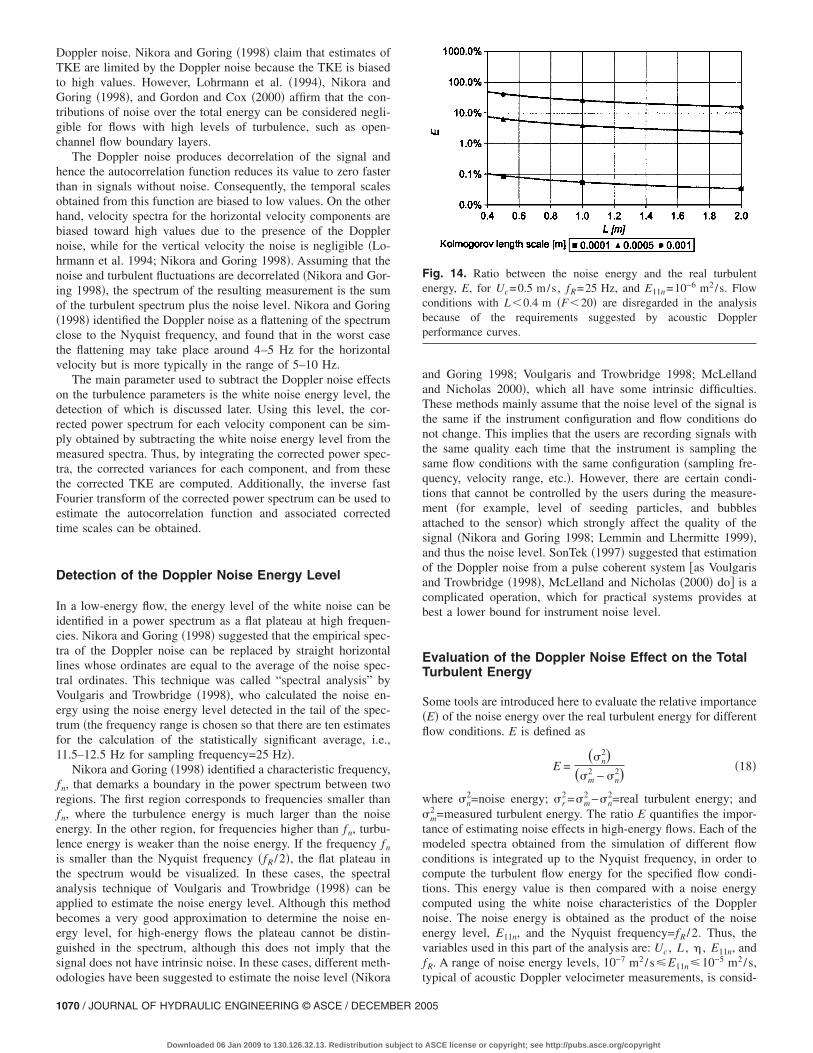
Fig. 14. Ratio between the noise energy and the real turbulentenergy, E, for Uc=0.5 m/s , fR=25 Hz, and E11n=10−6 m2/s. Flowconditions with L�0.4 m �F�20� are disregarded in the analysisbecause of the requirements suggested by acoustic Dopplerperformance curves.

typical of acoustic Doppler velocimeter measurements, is consid-

05


ered here based on experience and previous research �Nikora andGoring 1998�.

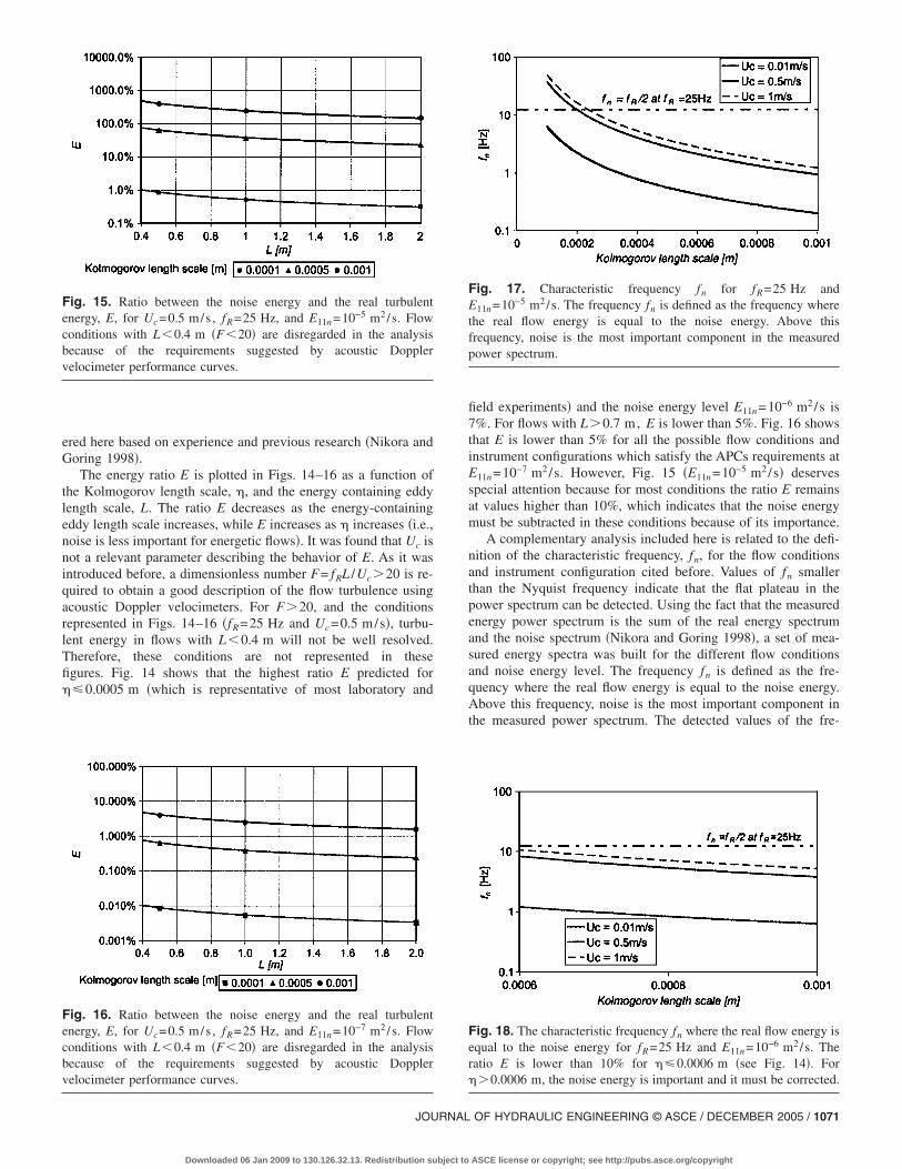
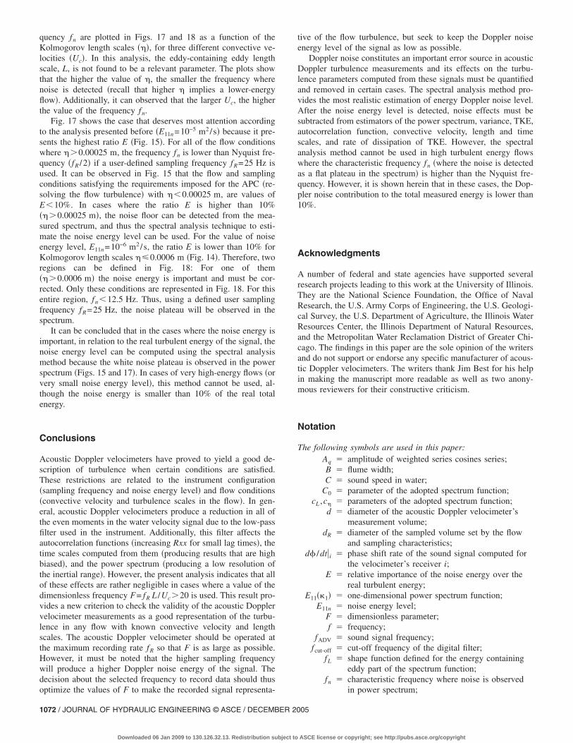
The energy ratio E is plotted in Figs. 14–16 as a function ofthe Kolmogorov length scale, �, and the energy containing eddylength scale, L. The ratio E decreases as the energy-containingeddy length scale increases, while E increases as � increases �i.e.,noise is less important for energetic flows�. It was found that Uc isnot a relevant parameter describing the behavior of E. As it wasintroduced before, a dimensionless number F= fRL /Uc�20 is re-quired to obtain a good description of the flow turbulence usingacoustic Doppler velocimeters. For F�20, and the conditionsrepresented in Figs. 14–16 �fR=25 Hz and Uc=0.5 m/s�, turbu-lent energy in flows with L�0.4 m will not be well resolved.Therefore, these conditions are not represented in thesefigures. Fig. 14 shows that the highest ratio E predicted for��0.0005 m �which is representative of most laboratory and

Fig. 15. Ratio between the noise energy and the real turbulentenergy, E, for Uc=0.5 m/s , fR=25 Hz, and E11n=10−5 m2/s. Flowconditions with L�0.4 m �F�20� are disregarded in the analysisbecause of the requirements suggested by acoustic Dopplervelocimeter performance curves.

Fig. 16. Ratio between the noise energy and the real turbulentenergy, E, for Uc=0.5 m/s , fR=25 Hz, and E11n=10−7 m2/s. Flowconditions with L�0.4 m �F�20� are disregarded in the analysisbecause of the requirements suggested by acoustic Dopplervelocimeter performance curves.

JOURNAL


field experiments� and the noise energy level E11n=10−6 m2/s is7%. For flows with L�0.7 m, E is lower than 5%. Fig. 16 showsthat E is lower than 5% for all the possible flow conditions andinstrument configurations which satisfy the APCs requirements atE11n=10−7 m2/s. However, Fig. 15 �E11n=10−5 m2/s� deservesspecial attention because for most conditions the ratio E remainsat values higher than 10%, which indicates that the noise energymust be subtracted in these conditions because of its importance.

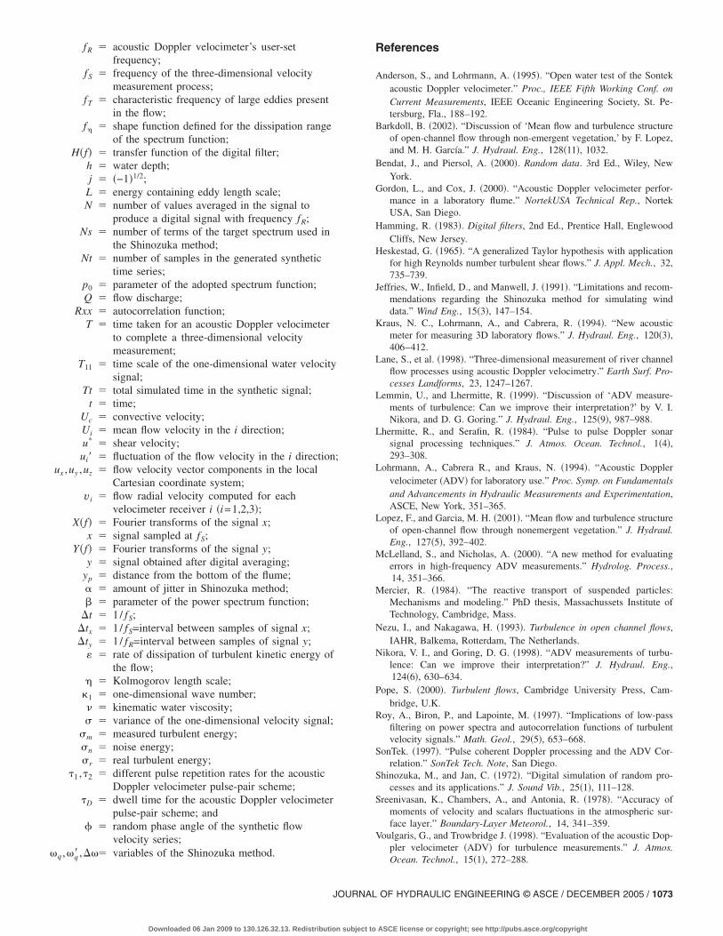
A complementary analysis included here is related to the defi-nition of the characteristic frequency, fn, for the flow conditionsand instrument configuration cited before. Values of fn smallerthan the Nyquist frequency indicate that the flat plateau in thepower spectrum can be detected. Using the fact that the measuredenergy power spectrum is the sum of the real energy spectrumand the noise spectrum �Nikora and Goring 1998�, a set of mea-sured energy spectra was built for the different flow conditionsand noise energy level. The frequency fn is defined as the fre-quency where the real flow energy is equal to the noise energy.Above this frequency, noise is the most important component inthe measured power spectrum. The detected values of the fre-

Fig. 17. Characteristic frequency fn for fR=25 Hz andE11n=10−5 m2/s. The frequency fn is defined as the frequency wherethe real flow energy is equal to the noise energy. Above thisfrequency, noise is the most important component in the measuredpower spectrum.

Fig. 18. The characteristic frequency fn where the real flow energy isequal to the noise energy for fR=25 Hz and E11n=10−6 m2/s. Theratio E is lower than 10% for ��0.0006 m �see Fig. 14�. For��0.0006 m, the noise energy is important and it must be corrected.



quency fn are plotted in Figs. 17 and 18 as a function of theKolmogorov length scales ��, for three different convective ve-locities �Uc�. In this analysis, the eddy-containing eddy lengthscale, L, is not found to be a relevant parameter. The plots showthat the higher the value of �, the smaller the frequency wherenoise is detected �recall that higher � implies a lower-energyflow�. Additionally, it can observed that the larger Uc, the higherthe value of the frequency fn.

Fig. 17 shows the case that deserves most attention accordingto the analysis presented before �E11n=10−5 m2/s� because it pre-sents the highest ratio E �Fig. 15�. For all of the flow conditionswhere ��0.00025 m, the frequency fn is lower than Nyquist fre-quency �fR /2� if a user-defined sampling frequency fR=25 Hz isused. It can be observed in Fig. 15 that the flow and samplingconditions satisfying the requirements imposed for the APC �re-solving the flow turbulence� with ��0.00025 m, are values ofE�10%. In cases where the ratio E is higher than 10%��0.00025 m�, the noise floor can be detected from the mea-sured spectrum, and thus the spectral analysis technique to esti-mate the noise energy level can be used. For the value of noiseenergy level, E11n=10−6 m2/s, the ratio E is lower than 10% forKolmogorov length scales ��0.0006 m �Fig. 14�. Therefore, tworegions can be defined in Fig. 18: For one of them��0.0006 m� the noise energy is important and must be cor-rected. Only these conditions are represented in Fig. 18. For thisentire region, fn�12.5 Hz. Thus, using a defined user samplingfrequency fR=25 Hz, the noise plateau will be observed in thespectrum.

It can be concluded that in the cases where the noise energy isimportant, in relation to the real turbulent energy of the signal, thenoise energy level can be computed using the spectral analysismethod because the white noise plateau is observed in the powerspectrum �Figs. 15 and 17�. In cases of very high-energy flows �orvery small noise energy level�, this method cannot be used, al-though the noise energy is smaller than 10% of the real totalenergy.

Conclusions

Acoustic Doppler velocimeters have proved to yield a good de-scription of turbulence when certain conditions are satisfied.These restrictions are related to the instrument configuration�sampling frequency and noise energy level� and flow conditions�convective velocity and turbulence scales in the flow�. In gen-eral, acoustic Doppler velocimeters produce a reduction in all ofthe even moments in the water velocity signal due to the low-passfilter used in the instrument. Additionally, this filter affects theautocorrelation functions �increasing Rxx for small lag times�, thetime scales computed from them �producing results that are highbiased�, and the power spectrum �producing a low resolution ofthe inertial range�. However, the present analysis indicates that allof these effects are rather negligible in cases where a value of thedimensionless frequency F= fR L /Uc�20 is used. This result pro-vides a new criterion to check the validity of the acoustic Dopplervelocimeter measurements as a good representation of the turbu-lence in any flow with known convective velocity and lengthscales. The acoustic Doppler velocimeter should be operated atthe maximum recording rate fR so that F is as large as possible.However, it must be noted that the higher sampling frequencywill produce a higher Doppler noise energy of the signal. Thedecision about the selected frequency to record data should thus
optimize the values of F to make the recorded signal representa-


tive of the flow turbulence, but seek to keep the Doppler noiseenergy level of the signal as low as possible.

Doppler noise constitutes an important error source in acousticDoppler turbulence measurements and its effects on the turbu-lence parameters computed from these signals must be quantifiedand removed in certain cases. The spectral analysis method pro-vides the most realistic estimation of energy Doppler noise level.After the noise energy level is detected, noise effects must besubtracted from estimators of the power spectrum, variance, TKE,autocorrelation function, convective velocity, length and timescales, and rate of dissipation of TKE. However, the spectralanalysis method cannot be used in high turbulent energy flowswhere the characteristic frequency fn �where the noise is detectedas a flat plateau in the spectrum� is higher than the Nyquist fre-quency. However, it is shown herein that in these cases, the Dop-pler noise contribution to the total measured energy is lower than10%.

Acknowledgments

A number of federal and state agencies have supported severalresearch projects leading to this work at the University of Illinois.They are the National Science Foundation, the Office of NavalResearch, the U.S. Army Corps of Engineering, the U.S. Geologi-cal Survey, the U.S. Department of Agriculture, the Illinois WaterResources Center, the Illinois Department of Natural Resources,and the Metropolitan Water Reclamation District of Greater Chi-cago. The findings in this paper are the sole opinion of the writersand do not support or endorse any specific manufacturer of acous-tic Doppler velocimeters. The writers thank Jim Best for his helpin making the manuscript more readable as well as two anony-mous reviewers for their constructive criticism.

Notation

The following symbols are used in this paper:Aq � amplitude of weighted series cosines series;B � flume width;C � sound speed in water;

C0 � parameter of the adopted spectrum function;cL ,c� � parameters of the adopted spectrum function;

d � diameter of the acoustic Doppler velocimeter’smeasurement volume;

dR � diameter of the sampled volume set by the flowand sampling characteristics;

d� /dt�i � phase shift rate of the sound signal computed forthe velocimeter’s receiver i;

E � relative importance of the noise energy over thereal turbulent energy;

E11�1� � one-dimensional power spectrum function;E11n � noise energy level;

F � dimensionless parameter;f � frequency;

fADV � sound signal frequency;fcut-off � cut-off frequency of the digital filter;

fL � shape function defined for the energy containingeddy part of the spectrum function;

fn � characteristic frequency where noise is observed
in power spectrum;
05


fR � acoustic Doppler velocimeter’s user-setfrequency;

fS � frequency of the three-dimensional velocitymeasurement process;

fT � characteristic frequency of large eddies presentin the flow;

f� � shape function defined for the dissipation rangeof the spectrum function;

H�f� � transfer function of the digital filter;h � water depth;j � �−1�1/2;

L � energy containing eddy length scale;N � number of values averaged in the signal to

produce a digital signal with frequency fR;Ns � number of terms of the target spectrum used in

the Shinozuka method;Nt � number of samples in the generated synthetic

time series;p0 � parameter of the adopted spectrum function;Q � flow discharge;

Rxx � autocorrelation function;T � time taken for an acoustic Doppler velocimeter

to complete a three-dimensional velocitymeasurement;

T11 � time scale of the one-dimensional water velocitysignal;

Tt � total simulated time in the synthetic signal;t � time;

Uc � convective velocity;Ui � mean flow velocity in the i direction;u* � shear velocity;ui� � fluctuation of the flow velocity in the i direction;

ux ,uy ,uz � flow velocity vector components in the localCartesian coordinate system;

vi � flow radial velocity computed for eachvelocimeter receiver i �i=1,2,3�;

X�f� � Fourier transforms of the signal x;x � signal sampled at fS;

Y�f� � Fourier transforms of the signal y;y � signal obtained after digital averaging;

yp � distance from the bottom of the flume; � amount of jitter in Shinozuka method; � parameter of the power spectrum function;

�t � 1/ fS;�tx � 1/ fS=interval between samples of signal x;�ty � 1/ fR=interval between samples of signal y;

� � rate of dissipation of turbulent kinetic energy ofthe flow;

� � Kolmogorov length scale;1 � one-dimensional wave number;� � kinematic water viscosity;� � variance of the one-dimensional velocity signal;

�m � measured turbulent energy;�n � noise energy;�r � real turbulent energy;

�1 ,�2 � different pulse repetition rates for the acousticDoppler velocimeter pulse-pair scheme;

�D � dwell time for the acoustic Doppler velocimeterpulse-pair scheme; and

� � random phase angle of the synthetic flowvelocity series;

�q ,�q� ,�� variables of the Shinozuka method.

JOURNAL


References

Anderson, S., and Lohrmann, A. �1995�. “Open water test of the Sontekacoustic Doppler velocimeter.” Proc., IEEE Fifth Working Conf. onCurrent Measurements, IEEE Oceanic Engineering Society, St. Pe-tersburg, Fla., 188–192.

Barkdoll, B. �2002�. “Discussion of ‘Mean flow and turbulence structureof open-channel flow through non-emergent vegetation,’ by F. Lopez,and M. H. García.” J. Hydraul. Eng., 128�11�, 1032.

Bendat, J., and Piersol, A. �2000�. Random data. 3rd Ed., Wiley, NewYork.

Gordon, L., and Cox, J. �2000�. “Acoustic Doppler velocimeter perfor-mance in a laboratory flume.” NortekUSA Technical Rep., NortekUSA, San Diego.

Hamming, R. �1983�. Digital filters, 2nd Ed., Prentice Hall, EnglewoodCliffs, New Jersey.

Heskestad, G. �1965�. “A generalized Taylor hypothesis with applicationfor high Reynolds number turbulent shear flows.” J. Appl. Mech., 32,735–739.

Jeffries, W., Infield, D., and Manwell, J. �1991�. “Limitations and recom-mendations regarding the Shinozuka method for simulating winddata.” Wind Eng., 15�3�, 147–154.

Kraus, N. C., Lohrmann, A., and Cabrera, R. �1994�. “New acousticmeter for measuring 3D laboratory flows.” J. Hydraul. Eng., 120�3�,406–412.

Lane, S., et al. �1998�. “Three-dimensional measurement of river channelflow processes using acoustic Doppler velocimetry.” Earth Surf. Pro-cesses Landforms, 23, 1247–1267.

Lemmin, U., and Lhermitte, R. �1999�. “Discussion of ‘ADV measure-ments of turbulence: Can we improve their interpretation?’ by V. I.Nikora, and D. G. Goring.” J. Hydraul. Eng., 125�9�, 987–988.

Lhermitte, R., and Serafin, R. �1984�. “Pulse to pulse Doppler sonarsignal processing techniques.” J. Atmos. Ocean. Technol., 1�4�,293–308.

Lohrmann, A., Cabrera R., and Kraus, N. �1994�. “Acoustic Dopplervelocimeter �ADV� for laboratory use.” Proc. Symp. on Fundamentalsand Advancements in Hydraulic Measurements and Experimentation,ASCE, New York, 351–365.

Lopez, F., and Garcia, M. H. �2001�. “Mean flow and turbulence structureof open-channel flow through nonemergent vegetation.” J. Hydraul.Eng., 127�5�, 392–402.

McLelland, S., and Nicholas, A. �2000�. “A new method for evaluatingerrors in high-frequency ADV measurements.” Hydrolog. Process.,14, 351–366.

Mercier, R. �1984�. “The reactive transport of suspended particles:Mechanisms and modeling.” PhD thesis, Massachussets Institute ofTechnology, Cambridge, Mass.

Nezu, I., and Nakagawa, H. �1993�. Turbulence in open channel flows,IAHR, Balkema, Rotterdam, The Netherlands.

Nikora, V. I., and Goring, D. G. �1998�. “ADV measurements of turbu-lence: Can we improve their interpretation?” J. Hydraul. Eng.,124�6�, 630–634.

Pope, S. �2000�. Turbulent flows, Cambridge University Press, Cam-bridge, U.K.

Roy, A., Biron, P., and Lapointe, M. �1997�. “Implications of low-passfiltering on power spectra and autocorrelation functions of turbulentvelocity signals.” Math. Geol., 29�5�, 653–668.

SonTek. �1997�. “Pulse coherent Doppler processing and the ADV Cor-relation.” SonTek Tech. Note, San Diego.

Shinozuka, M., and Jan, C. �1972�. “Digital simulation of random pro-cesses and its applications.” J. Sound Vib., 25�1�, 111–128.

Sreenivasan, K., Chambers, A., and Antonia, R. �1978�. “Accuracy ofmoments of velocity and scalars fluctuations in the atmospheric sur-face layer.” Boundary-Layer Meteorol., 14, 341–359.

Voulgaris, G., and Trowbridge J. �1998�. “Evaluation of the acoustic Dop-pler velocimeter �ADV� for turbulence measurements.” J. Atmos.Ocean. Technol., 15�1�, 272–288.



Download - Turbulence Measurements with Acoustic Doppler …laboratorios.fi.uba.ar/mincyt/docs/1288320366.pdf · S/2 Nyquist theorem, see Bendat and Piersol 2000 . This indicates that energy

Top Related