Statistical Methods for Computational
Biology
Sayan Mukherjee


Contents
Statistical Methods for Computational Biology 1
Lecture 1. Course preliminaries and overview 1
Lecture 2. Probability and statistics overview 32.1. Discrete random variables and distributions 3
Lecture 3. Hypothesis testing 25
3

Stat293 class notes
Statistical Methods for Computational
Biology
Sayan Mukherjee
LECTURE 1
Course preliminaries and overview
• Course summaryThe use of statistical methods and tools from applied probability to ad-dress problems in computational molecular biology. Biological problemsin sequence analysis, structure prediction, gene expression analysis, phy-logenetic trees, and statistical genetics will be addressed. The followingstatistical topics and techniques will be used to address the biologicalproblems: classical hypothesis testing, Bayesian hypothesis testing, Mul-tiple hypothesis testing, extremal statistics, Markov chains, continuousMarkov processes, Expectation Maximization and imputation, classifica-tion methods, and clustering methods. Along the way we’ll learn aboutgambling, card shuffling, and coin tossing.
• Grading
There will be four problem sets that will account for 40% of the grade,a midterm exam that will account for 20% of the grade, a final exam for40% of the grade (students that have an A after the midterm, both examand homeworks, will have an option to complete a final project in lieu ofthe final exam)
1Institute of Statistics and Decision Sciences (ISDS) and Institute for Genome Sciences and Policy(IGSP), Duke University, Durham, 27708.E-mail address: [email protected].
Dec 6, 2005
These lecture notes borrow heavily from many sources.
c©1993 American Mathematical Society
1

LECTURE 2
Probability and statistics overview
Throughout this course we will quantify, assess, explain noise and randomnessin (molecular) biological systems.
Two disciplines will play a prominent role:
• Probability: The word probability derives from the Latin probare (toprove, or to test). Informally, probable is one of several words applied touncertain events or knowledge, being more or less interchangeable withlikely, risky, hazardous, uncertain, and doubtful, depending on the con-text. Chance, odds, and bet are other words expressing similar notions.As with the theory of mechanics which assigns precise definitions to sucheveryday terms as work and force, so the theory of probability attemptsto quantify the notion of probable.
• Statistics:(1) The mathematics of the collection, organization, and interpretation
of numerical data, especially the analysis of population characteristicsby inference from sampling.
(2) Numerical data.(3) From German Statistik – political science, from New Latin statisticus
– of state affairs, from Italian statista – person skilled in statecraft,from stato, from Latin status – position, form of government.
(4) Inverse probability
2.1. Discrete random variables and distributions
Apology. This is not a math course so we will avoid formal mathematical defini-tions whenever possible.
2.1.1. Definitions
There exists a space of elementary events or outcomes of an experiment. The eventsare discrete (countable) and disjoint and we call this set Ω.
Examples. Coin tossing: My experiment is tossing (or spinning) a coin. Thereare two outcomes “heads” and “tails”. So Ω = heads, tails and |Ω| = 2.
3
4 S. MUKHERJEE, STATISTICS FOR COMP BIO
Dice rolling: My experiment is rolling a six sided die. So Ω = 1, 2, 3, 4, 5, 6and |Ω| = 6.
Waiting for tail: My experiment is to continually toss a coin until a tail showsup. If I designate heads as h and tails as t in a toss then an elementary outcomeof this experiment is a sequence of the form (hhhhh...ht). There are an infinitenumber of such sequences so I will not write Ω and we can state that |Ω| = ∞.
The space of elementary events is Ω and the elements of the space Ω are denotedas ω. Any subset A ⊆ Ω is also an event (the event A occurs if any of the elementaryoutcomes ω ∈ A occur).
The sum of two events A and B is the event A ∪ B consist of elementaryoutcomes which belong to at least one of the events A and B. The product oftwo events A ∩ B consists of all events belonging to both A and B. The space Ωis the certain event. The empty set ∅ is the impossible event. A = Ω − A is thecomplementary event of A. Two events are mutually exclusive if A ∩ B = ∅.
Examples. For a single coin toss coins A = t and B = h are complementary andmutually exclusive, Ω − A = t and t ∩ h = ∅.
For a single dice role two possible events are A = 1 and B = 6 so A ∪ Bdesignates either a 1 or 6 is rolled.
Consider rolling a die twice the space of elementary events can be designated(i, j) where i, j = 1, ..., 6. The events A = i+j ≤ 3 and B = j = 6 are mutuallyexclusive. The product of events A and C = j is even is the event (1, 2).
A probability distribution assigns a nonnegative real number to each event A ⊆Ω. A probability distribution is a function Pr defined on Ω such that Pr : A → IR+
and
1 =∑
ω∈Ω
Pr(ω)
Pr(A) =∑
ω∈A
Pr(ω).
Examples. Symmetric die, one toss: Pr(1) = Pr(2) = Pr(3) = Pr(4) = Pr(5) =Pr(6) = 1
6 .
Symmetric coin, one toss: Pr(h) = Pr(t) = 12 .
Waiting for head, symmetric coin: Pr(h) = 12 , Pr(th) = 1
2
2, Pr(tth) = 1
2
3, ...
∑
ω∈Ω Pr(ω) =∑∞
n=1 2−n = 1 so we define a probability distribution on Ω. Theprobability the experiment stops at an even step (∪(th) ∪ (ttth) ∪ ...) is the sum ofthe corresponding probabilities
∑∞n=1 2−2n = 1
4 × 43 = 1
3 .
Properties of probabilities
(1) Pr(∅) = 0 and Pr(Ω) = 1(2) Pr(A+B) =
∑
ω∈A∪B Pr(ω) =∑
ω∈A Pr(ω)+∑
ω∈B Pr(ω)−∑ω∈A∩B Pr(ω) =Pr(A) + Pr(B) − Pr(AB)
(3) Pr(A) = 1 − Pr(A)(4) if A and B are disjoint events
Pr(A + B) = Pr(A) + Pr(B)
LECTURE 2. PROBABILITY AND STATISTICS OVERVIEW 5
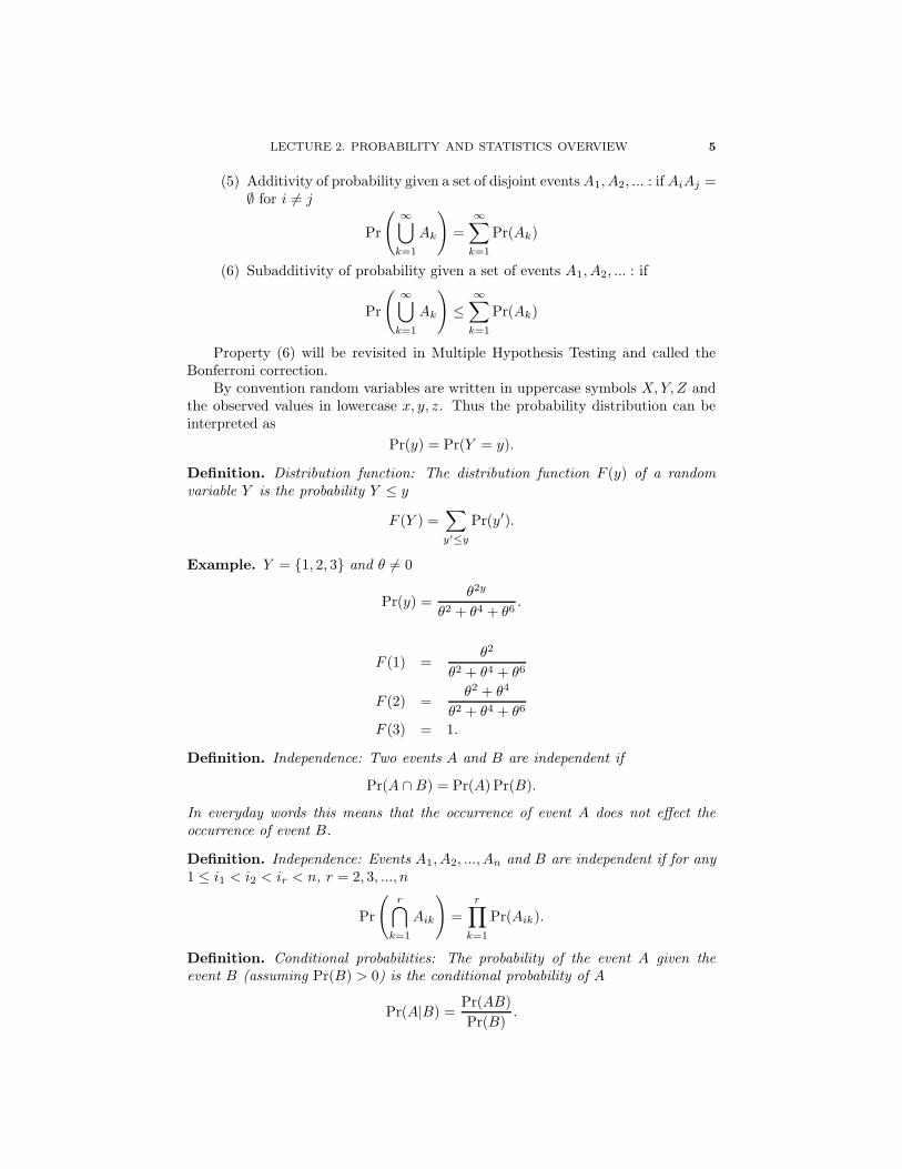
(5) Additivity of probability given a set of disjoint events A1, A2, ... : if AiAj =∅ for i 6= j
Pr
( ∞⋃
k=1
Ak
)
=
∞∑
k=1
Pr(Ak)
(6) Subadditivity of probability given a set of events A1, A2, ... : if
Pr
( ∞⋃
k=1
Ak
)
≤∞∑
k=1
Pr(Ak)
Property (6) will be revisited in Multiple Hypothesis Testing and called theBonferroni correction.
By convention random variables are written in uppercase symbols X, Y, Z andthe observed values in lowercase x, y, z. Thus the probability distribution can beinterpreted as
Pr(y) = Pr(Y = y).
Definition. Distribution function: The distribution function F (y) of a randomvariable Y is the probability Y ≤ y
F (Y ) =∑
y′≤y
Pr(y′).
Example. Y = 1, 2, 3 and θ 6= 0
Pr(y) =θ2y
θ2 + θ4 + θ6.
F (1) =θ2
θ2 + θ4 + θ6
F (2) =θ2 + θ4
θ2 + θ4 + θ6
F (3) = 1.
Definition. Independence: Two events A and B are independent if
Pr(A ∩ B) = Pr(A) Pr(B).
In everyday words this means that the occurrence of event A does not effect theoccurrence of event B.
Definition. Independence: Events A1, A2, ..., An and B are independent if for any1 ≤ i1 < i2 < ir < n, r = 2, 3, ..., n
Pr
(
r⋂
k=1
Aik
)
=r∏
k=1
Pr(Aik).
Definition. Conditional probabilities: The probability of the event A given theevent B (assuming Pr(B) > 0) is the conditional probability of A
Pr(A|B) =Pr(AB)
Pr(B).
6 S. MUKHERJEE, STATISTICS FOR COMP BIO
Example. We toss two fair coins. Let event A be the event that the first tossresults in heads, and event B the event that tails shows up on the second toss
Pr(AB) =1
4=
1
2× 1
2= Pr(A) Pr(B).
We have a die that is tetrahedron (Dungeons and Dragons for example) withthree faces painted red, blue, and green respectively, and the fourth in all threecolors. We roll the die. Event R is that the bottom face is red, event B that itis blue, and event G it is green. Pr(R) = Pr(B) = Pr(G) = 2
4 = 12 . Pr(RB) =
Pr(GB) = Pr(GR) = ... = 12 × 1
2 = 14 . However,
Pr(RGB) =1
46== Pr(R) Pr(G) Pr(B) =
1
8.
Definition. Given two integers n, i with i ≤ n the number of ways i integers canbe selected from n integers irrespective of order is
(
n
i
)
=n!
(n − i)! i!.
This is often stated as n choose i.
2.1.2. My favorite discrete distributions
(1) Bernoulli trials: A single trial (coin flip) with two outcomes Ω = failure, success.The probability of success is p and therefore failure is 1 − p.
If we assign to a Bernoulli random variable Y the number of successesin a trial the Y = 0 with probability 1 − p and Y = 1 with p and
Pr(y) = py(1 − p)1−y, y = 0, 1.
If we assign to a Bernoulli random variable S the value −1 if the trialresults in failure and +1 if it results in success then
Pr(s) = p(1+s)/2(1 − p)(1−s)/2, s = −1, 1.
(2) Binomial distribution: A binomial random variable is the number of suc-cesses of n independent and identical Bernoulli trials. Identical Bernoullitrials means that the distribution function is identical for each trial orthat each trial shares the same probability of success p. The two variablesn and p are the index and parameter for the distribution respectively. Theprobability distribution of Y is
Pr(y) =
(
n
y
)
py(1 − p)n−y, y = 1, 2, ..., n.
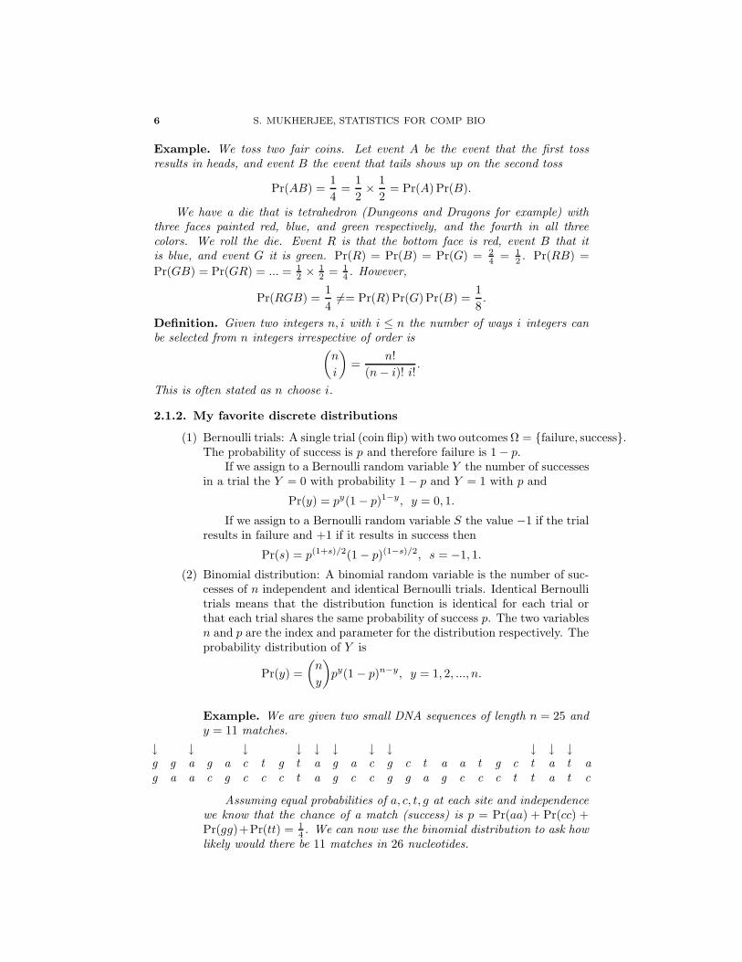
Example. We are given two small DNA sequences of length n = 25 andy = 11 matches.
↓ ↓ ↓ ↓ ↓ ↓ ↓ ↓ ↓ ↓ ↓g g a g a c t g t a g a c g c t a a t g c t a t ag a a c g c c c t a g c c g g a g c c c t t a t c
Assuming equal probabilities of a, c, t, g at each site and independencewe know that the chance of a match (success) is p = Pr(aa) + Pr(cc) +Pr(gg)+Pr(tt) = 1
4 . We can now use the binomial distribution to ask howlikely would there be 11 matches in 26 nucleotides.
LECTURE 2. PROBABILITY AND STATISTICS OVERVIEW 7
Is i.i.d. Bernoulli a good idea for nucleotides ?
(3) Uniform distribution: The random variable Y takes the possible valuesΩ = a, a+, ..., a + b − 1 or U [a, b) where a, b ∈ IN and
Pr(y) = b−1 for y = a, a + 1, ..., a + b − 1.
(4) Geometric distribution: We run a sequence of i.i.d. Bernoulli trials eachwith success p. The random variable of interest the number of trials Ybefore (but not including) the first failure. Again Y = 0, 1, 2, .... IfY = y then there must have been y successes followed by one failure sothe distribution is
Pr(y) = (1 − p)py, y = 0, 1, 2, ...
and the distribution function is
F (y) = Pr(Y ≤ y) = 1 − py+1, y = 0, 1, 2, ...
The length of (sssssssssssf) of Y is the length of a success run. Thistype of random variable will be used in computing probabilities randomof contiguous matches in the comparison of two sequences.
(5) Poisson Distribution: A random variable Y has a Poisson distribution(with parameter λ > 0) if
Pr(y) =e−λλy
y!, y = 0, 1, 2, ...
The Poisson Distribution can be derived as a limit of the binomial distribu-tion and will arise in many biological applications involving evolutionaryprocesses.
(6) Hypergeometric distribution: Jane ran a gene expression experiment whereshe measured the expression of n = 7, 000 genes, of these genes she foundthat n1 = 500 were biologically important via a high throughput drugscreen. Jane’s friend Olaf found k = 200 genes in a toxicity screen. Ifboth the toxicity screen and the drug screen are random and independentwith respect to the genes then the probability that there is an overlap ofk1 genes in the drug and toxicity screen lists is
Pr(n1, n, k1, k) =
(
n1
k1
)(
n − n1
k − k1
)
/
(
n
k
)
.
The classical formulation is with urns. Our urn contains n balls ofwhich n1 are black and the remaining n−n1 are white. We sample k ballsfrom the urn without replacement. What is the probability that there willbe exactly k1 black balls in the sample k.
Is the hypergeometric distribution a good idea to model Jane andOlaf’s problem ?
2.1.3. Means and variances of discrete random variables
Definition. The mean or expectation of a discrete random variable Y is
µ = IE[Y ] =∑
y
y Pr(y),
where the sum is over all possible values of Y .
8 S. MUKHERJEE, STATISTICS FOR COMP BIO
Example. Given a binomial random variable Y its mean is
µ = IE[Y ] =
n∑
y=0
y
(
n
y
)
py(1 − p)n−y = np.
Definition. The mean or expectation of function of discrete random variable f(Y )is
IE[f(Y )] =∑
y
f(y) Pr(y),
where the sum is over all possible values of Y .
Definition. Linearity: If Y us a discrete random variable and α and β are con-stants
IE[α + βY ] =∑
y
(α + βy) Pr(y) = α + βµ.
Definition. The variance of a discrete random variable Y is
σ2 = var[Y ] =∑
y
(y − µ)2 Pr(y),
where the sum is over all possible values of Y . The standard deviation is σ.
Definition. If Y us a discrete random variable and α and β are constants
var[α + βY ] = β2σ2.
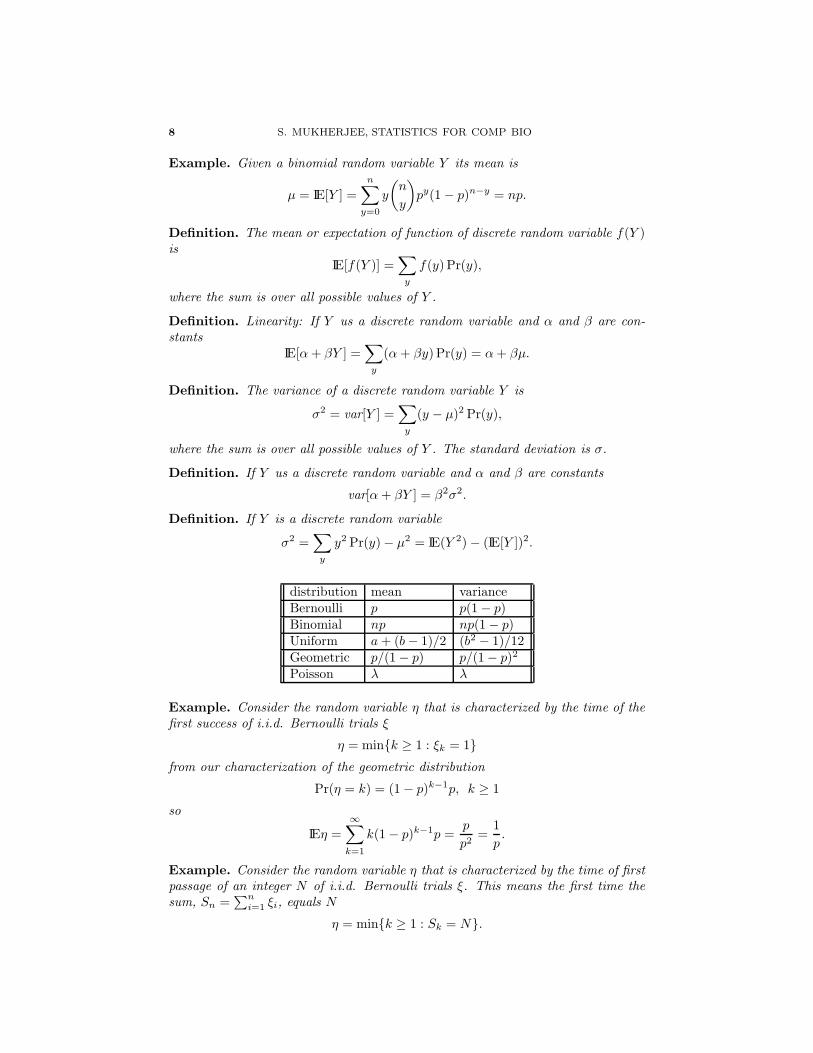
Definition. If Y is a discrete random variable
σ2 =∑
y
y2 Pr(y) − µ2 = IE(Y 2) − (IE[Y ])2.
distribution mean varianceBernoulli p p(1 − p)Binomial np np(1 − p)Uniform a + (b − 1)/2 (b2 − 1)/12Geometric p/(1 − p) p/(1− p)2
Poisson λ λ
Example. Consider the random variable η that is characterized by the time of thefirst success of i.i.d. Bernoulli trials ξ
η = mink ≥ 1 : ξk = 1from our characterization of the geometric distribution
Pr(η = k) = (1 − p)k−1p, k ≥ 1
so
IEη =∞∑
k=1
k(1 − p)k−1p =p
p2=
1
p.
Example. Consider the random variable η that is characterized by the time of firstpassage of an integer N of i.i.d. Bernoulli trials ξ. This means the first time thesum, Sn =
∑ni=1 ξi, equals N
η = mink ≥ 1 : Sk = N.

LECTURE 2. PROBABILITY AND STATISTICS OVERVIEW 9
The probability distribution for η can be defined recursively
Pr(η = k) = p × Pr(Sk−1 = N − 1),
and the expectation is
IEη = p ×∞∑
k=N
k
(
k − 1
N − 1
)
pN−1(1 − p)k−N
=pN
(N − 1)!
∞∑
k=N
k(k − 1) · · · (k − N + 1)(1 − p)k−N .
2.1.4. Moments of distributions and generating functions
Definition. If Y is a discrete random variable then IE(Y r) is the rth moment and
IE(Y r) =∑
y
yr Pr(y).
Definition. If Y is a discrete random variable then the rth moment about the meanis moment and
µr =∑
y
(y − µ)r Pr(y).
The first such moment is zero, the second is the variance σ2 the third is theskewness and the fourth is the kurtosis.
For a discrete random variable the probability generating function pgf will bedenoted q(t) and is defined as
q(t) = IE[
tY]
=∑
y
tyP (y).
Examples. For the Bernoulli random variable
Pr(y) = py(1 − p)1−y, y = 0, 1,
the pgf isq(t) = 1 − p + pt.
For the Bernoulli random variable
Pr(s) = p(1+s)/2(1 − p)(1−s)/2, s = −1, 1,
the pgf isq(t) = (1 − p)t−1 + pt.
For the binomial random variable
Pr(y) =
(
n
y
)
py(1 − p)n−y, y = 1, 2, ..., n,
the pgf isq(t) = (1 − p + pt)n.
The pgf can be used to derive moments of a probability distribution
µ =
(
d
dtq(t)
)
t=1
σ =
(
d2
dt2q(t)
)
t=1
+ µ − µ2
10 S. MUKHERJEE, STATISTICS FOR COMP BIO
Theorem. If two random variables have pgfs q1(t) and q2(t) and both pgfs convergein some open interval I containing 1. If q1(t) = q2(t) for all t ∈ I, then the tworandom variables have the identical distributions.
2.1.5. Continuous random variables
Some random variables are continuous rather than discrete. For example, amountof protein expressed or concentration of an enzyme are continuous valued. Againwe use uppercase letters, X, Y, Z, for the random variable and lowercase letters,x, y, z, for values the random variable takes. A continuous random variable takesvalues over a range −∞ < X < ∞ or L < ∞X < H . Continuous random variablesare associated with a probability density function p(x) for which
Pr(a < X < b) =
∫ b
a
p(x)dx,
and
p(x) = limh→0
Pr(x < X < x + h)
h,
and a (cumulative) distribution function
F (x) =
∫ x
−∞p(u)du,
it is clear that 0 ≤ F (x) ≤ 1 and by calculus (the Radon-Nikodym Theorem)
p(x) =d
dxF (x).
Definition. The mathematical mean or expectation of a random variable X is
µ = IEX =
∫ ∞
−∞xp(x)dx =
∫ ∞
−∞xdF (x).
The mean is in some sense the “center of mass” of the distribution F (x). Instatistics it is often called a location parameter of the distribution. The followingproperties are a result of the linearity of expectations and Fubini’s theorem
(1) IE(a + bX) = a + bµ(2) IE(X + Y ) = IEX + IEY(3) If a ≤ X ≤ B then a ≤ IEX ≤ b(4) The probability of an event A can be expressed in terms of expectations
of an indicator random variable
Pr(A) = IEI(A),
where the indicator function I(A) is 1 if A = true and 0 otherwise.
Definition. The variance of a random variable X is
σ2 = IE(X − µ)2 =
∫ ∞
−∞(x − µ)2p(x)dx = IEX2 − (IEX)2 = min
aIE(X − a)2.
The variance is the amount of dispersion or concentration of the mass of thedistribution about the mean. In statistics it is often called a scale parameter of thedistribution.

LECTURE 2. PROBABILITY AND STATISTICS OVERVIEW 11
Definition. The variance of a random variable X is
σ2 = IE(X − µ)2 =
∫ ∞
−∞(x − µ)2p(x)dx = IEX2 − (IEX)2 = min
aIE(X − a)2.
The second moment of a zero mean random variable is its variance.
Definition. The r-th moment of a random variable X is
IEXr =
∫ ∞
−∞xrp(x)dx.
Definition. The centered r-th moment of a random variable X is
IE(X − µ)r =
∫ ∞
−∞(x − µ)rp(x)dx.
All the above can be defined for a function f(X) of a random variable
IEf(x) = IEx∼X [f(x)] =
∫
x
f(x)p(x)dx.
Example. Our objective is to diagnose whether a patient has lung cancer type Aor lung cancer type B. We measure the expression level of 3, 000 genes for eachpatient, X ∈ IR3,000. The patients cancer type can be designated as Y ∈ A, B.Patients with lung cancer type A have density function pA(x) = p(x|A) and thosewith lung cancer type B have density function pB(x) = P (x|B). The likelihoodof developing lung cancer A and B are equal. Assume an oracle gives us p(x|A)and p(x|B) our goal is to find an optimal classification function and state what itserror is. A classification function c is a map c : X → A, B and the error of aclassification function will be
Err[c] = IEx∼X,y∼Y [c(x) 6= y]
=
∫
X,Y
[c(x) 6= y]p(x, y)dxdy
=
∫
X
([c(x) 6= A]p(x, A)dx + [c(x) 6= B]p(x, B))dx,
a classification function that minimizes this error is called a Bayes optimal classifierand this minimum error is called the Bayes error.
Assume an oracle has given us pA(x) and pB(x) we can now compute the con-ditional probabilities (likelihoods):
Pr(A|x) =p(x, A)
p(x)=
p(x|A)p(A)
p(x),
Pr(B|x) =p(x, B)
p(x)=
p(x|B)p(B)
p(x).
We first compute p(x)
p(x) = p(x|A)p(A) + p(x|B)p(B),
which we can compute since we know p(x|A) and p(x|B) and p(A) = p(B) = 12 .
A the following function c∗ is a Bayes optimal classifier
c∗(x) =
A if p(A|x) ≥ p(B|x),
B o.w.
12 S. MUKHERJEE, STATISTICS FOR COMP BIO
2.1.6. Empirical distributions
In the previous section we defined continuous random variables and the previousexample demonstrated how we can characterize important aspects of a problemgiven a distribution.
However, in most real problems we are not given the distribution p(x) we areusually given a finite sample of n observations (x1, ..., xn) drawn from the distribu-tion p(x). We have to make use of the sample values as a proxy for the distributionp(x). This is done via the empirical distribution function.
Definition. Given a draw (x1, ..., xn) of n observations from p(x) we define theempirical distribution as
pn(x) =1
n
n∑
i=1
δ(xi),
where δ(·) is the delta function.
Definition. The delta function δ(x) is a function with the following property
g(x) =
∫
g(u)δ(x − u)du,
in that it “picks” out a function value at x.
Examples. An example of a delta function is the following
δ(x) = limσ→0
1
σ√
2πe−|x|/2σ2
.
Another example is
δ(x) = lima→0
1
aI(
x ∈[
x − a
2, x +
a
2
])
.
Given the empirical distribution we can define the sample average or averageas an expectation.
Definition. The sample average or average, µn, of a draw (x1, ..., xn) is
µn = IEnx =
∫
xpn(x)dx
=1
n
n∑
i=1
∫
x
xδ(xi)dx
=1
n
n∑
i=1
xi.
In general we will use quantities like µn as proxy for µ and this will be developedin the next section.
Example. We revisit example 2.1.5 we we were classifying patients as having lungcancer of type A or type B. We formulated the Bayes optimal classifier and the errorof the Bayes optimal classifier. In that example we were given p(x|A) and p(x|B) byan oracle. In real life we are given in general n observations ((x1, A), ...., (xn, A))from p(x|A) and n observations ((xn+1, B), ...., (x2n, B)) from p(x|B) this defines

LECTURE 2. PROBABILITY AND STATISTICS OVERVIEW 13
an empirical distribution function p2n(x, y). We can use this distribution functionto measure the empirical error of a classifier c
Err2n
[c] = IE2n[c(x) 6= y]
=
∫
X,Y
[c(x) 6= y]p2n(x, y)dxdy
=1
2n
[
n∑
i=1
[c(xi) 6= A] +
2n∑
i=n+1
[c(xi) 6= B]
]
.
An important question that we will focus on in the next section is how close areErr
2n[c] and Err[c].
2.1.7. Central limit theorems and law of large numbers
The main question addressed in this section is how close in µn to µ. We will alsomotivate why we ask this question.
A sequence of random variables yn converges almost surely to a random variableY iff IP(yn → Y ) = 1. A sequence of random variables yn converges in probabilityto a random variable Y iff for every ε > 0, limn→∞ IP(|yn − Y | > ε) = 0. Letµn := n−1
∑ni=1 xn. The sequence x1, ..., xn satisfies the strong law of large numbers
if for some constant c, µn converges to c almost surely. The sequence x1, ..., xn
satisfies the weak law of large numbers iff for some constant c, µn converges toc in probability. In general the constant c will be the expectation of the randomvariable IEx.
A given function f(x) of random variables x concentrates if the deviation be-tween its empirical average, n−1
∑ni=1 f(xi) and expectation, IEf(x), goes to zero
as n goes to infinity. That is f(x) satisfies the law of large numbers.
Theorem (Jensen). If φ is a convex function then φ(IEx) ≤ IEφ(x).
Theorem (Bienayme-Chebyshev). For any random variable x, ε > 0
Pr(|x| ≥ ε) ≤ IEx2
ε2.
Proof.
IEx2 ≥ IE(x2I(|x| ≥ ε)) ≥ ε2 Pr(|x| > ε).
Theorem (Chebyshev). For any random variable x, ε > 0
Pr(|x − µ| ≥ ε) ≤ Var(x)
ε2.
Proof. Same as above.
Theorem (Markov). For any random variable x, ε > 0
Pr(|x| ≥ ε) ≤ IEeλx
eλε
and
Pr(|x| ≥ ε) ≤ infλ<0
e−λεIEeλx.
14 S. MUKHERJEE, STATISTICS FOR COMP BIO
Proof.
Pr(x > ε) = Pr(eλx > eλε) ≤ IEeλx
eλε.
For the sums or averages of independent random variables the above boundscan be improved from polynomial in 1/ε to exponential in ε.
The following theorems will be for zero mean random variables. The extensionto nonzero mean is trivial.
Theorem (Bennet). Let x1, ..., xn be independent random variables with IEx = 0,IEx2 = σ2, and |xi| ≤ M . For ε > 0
Pr
(
|n∑
i=1
xi| > ε
)
≤ 2e−nσ2
M2 φ( εMnσ2 ),
where
φ(z) = (1 + z) log(1 + z) − z.
Proof. We will prove a bound on one-side of the above theorem
Pr
(
n∑
i=1
xi > ε
)
.
Pr
(
n∑
i=1
xi > ε
)
≤ e−λεIEeλP
xi = e−λεΠni=1IEeλxi
= e−λε(IEeλx)n.
IEeλx = IE∞∑
k=0
(λx)k
k!=
∞∑
k=0
λk IExk
k!
= 1 +
∞∑
k=2
λk
k!IEx2xk−2 ≤ 1 +
∞∑
k=2
λk
k!Mk−2σ2
= 1 +σ2
M2
∞∑
k=2
λkMk
k!= 1 +
σ2
M2(eλM − 1 − λM)
≤ eσ2
M2 (eλM−λM−1).
The last line holds since 1 + x ≤ ex.Therefore,
(2.1) Pr
(
n∑
i=1
xi > ε
)
≤ e−λεeσ2
M2 (eλM−λM−1).
We now optimize with respect to λ by taking the derivative with respect to λ
0 = −ε +nσ2
M2(MeλM − M),
eλM =εM
nσ2+ 1,
λ =1
Mlog
(
1 +εM
nσ2
)
.

LECTURE 2. PROBABILITY AND STATISTICS OVERVIEW 15
The theorem is proven by substituting λ into equation (2.1).
The problem with Bennet’s inequality is that it is hard to get a simple expres-sion for ε as a function of the probability of the sum exceeding ε.
Theorem (Bernstein). Let x1, ..., xn be independent random variables with IEx = 0,IEx2 = σ2, and |xi| ≤ M . For ε > 0
Pr
(
|n∑
i=1
xi| > ε
)
≤ 2e− ε2
2nσ2+23
εM .
Proof.Take the proof of Bennet’s inequality and notice
φ(z) ≥ z2
2 + 23z
.
Remark. With Bernstein’s inequality a simple expression for ε as a function ofthe probability of the sum exceeding ε can be computed
n∑
i=1
xi ≤2
3uM +
√2nσ2u.
Outline.
Pr
(
n∑
i=1
xi > ε
)
≤ 2e− ε2
2nσ2+ 23
εM = e−u,
where
u =ε2
2nσ2 + 23εM
.
we now solve for ε
ε2 − 2
3εM − 2nσ2ε = 0
and
ε =1
3uM +
√
u2M2
9+ 2nσ2u.
Since√
a + b ≤ √a +
√b
ε =2
3uM +
√2nσ2u.
So with large probabilityn∑
i=1
xi ≤2
3uM +
√2nσ2u. 4
If we want to bound
|µn − µ| = |n−1n∑
i=1
f(xi) − IEf(x)|
we consider|f(xi) − IEf(x)| ≤ 2M.
Thereforen∑
i=1
(f(xi) − IEf(x)) ≤ 4
3uM +
√2nσ2u
16 S. MUKHERJEE, STATISTICS FOR COMP BIO
and
n−1n∑
i=1
f(xi) − IEf(x) ≤ 4
3
uM
n+
√
2σ2u
n.
Similarly,
IEf(x) − n−1n∑
i=1
f(xi) ≥4
3
uM
n+
√
2σ2u
n.
In the above bound√
2σ2u
n≥ 4uM
n
which implies u ≤ nσ2
8M2 and therefore
|n−1n∑
i=1
f(xi) − IEf(x)| .
√
2σ2u
nfor u . nσ2,
which corresponds to the tail probability for a Gaussian random variable and ispredicted by the Central Limit Theorem (CLT) Condition that limn→∞ nσ2 → ∞.If limn→∞ nσ2 = C, where C is a fixed constant, then
|n−1n∑
i=1
f(xi) − IEf(x)| .C
n
which corresponds to the tail probability for a Poisson random variable.
Proposition. Bounds between the difference of sums of two draws of a randomvariable can be derived in the same manner as for the deviation between the sumand difference. This is called symmetrization in empirical process theory.
Given two draws from a distribution x1, ..., xn and x′1, ..., x
′n
Pr
(∣
∣
∣
∣
∣
1
n
n∑
i=1
f(xi) −1
n
n∑
i=1
f(x′i)
∣
∣
∣
∣
∣
≥ ε
)
≤ e− ε2n
8(2σ2+2Mε/2) .
Proof. From Bernstein’s inequality we know that
Pr
(∣
∣
∣
∣
∣
1
n
n∑
i=1
f(xi) − IEf(x)
∣
∣
∣
∣
∣
≥ ε
)
≤ 2e− ε2n
2σ2+2Mε/2 ,
Pr
(∣
∣
∣
∣
∣
1
n
n∑
i=1
f(x′i) − IEf(x)
∣
∣
∣
∣
∣
≥ ε
)
≤ 2e− ε2n
2σ2+2Mε/2 .
If we can ensure∣
∣
∣
∣
∣
1
n
n∑
i=1
f(xi) − IEf(x)
∣
∣
∣
∣
∣
≤ ε/2
∣
∣
∣
∣
∣
1
n
n∑
i=1
f(x′i) − IEf(x)
∣
∣
∣
∣
∣
≤ ε/2,
then∣
∣
∣
∣
∣
1
n
n∑
i=1
f(xi) −1
n
n∑
i=1
f(x′i)
∣
∣
∣
∣
∣
≤ ε.
Applying Bernstein’s inequality to the first two conditions gives us the desiredresult.

LECTURE 2. PROBABILITY AND STATISTICS OVERVIEW 17
Proposition. In addition to bounds on sums of random variables for certain distri-butions there also exist approximations to these sums. Let x1, ..., xn be independentrandom variables with IEx = 0, IEx2 = σ2, and |xi| ≤ M . For ε > 0
Pr
(
|n∑
i=1
xi| > ε
)
≈ Φ(ε, σ, n, M).
The approximations are computed using similar ideas as those in computing theupper bounds.
Example. Hypothesis testing is an example where limit distributions are applied.Assume we are given n observations from two experimental conditions x1, ..., xn
and z1, ..., zn.We ask the following question: are the means of the observations of the two
experimental conditions the same ?This is formulated as: can we reject the null hypothesis that the difference of
the means of the two two experimental conditions the same ?If x1, ..., xn and z1, ..., zn were drawn according to a distribution p(u) we would
know that
Pr
(∣
∣
∣
∣
∣
1
n
n∑
i=1
xi −1
n
n∑
i=1
zi
∣
∣
∣
∣
∣
≥ ε
)
≤ e− ε2n
8(2σ2+2Mε/2) .
So given the difference
d =1
n
n∑
i=1
xi −1
n
n∑
i=1
zi.
We can bound the probability this would occur by chance under the null hypothesis.Thus if d is very large the chance that the null hypothesis gave rise to d is smalland so we may reject the null hypothesis.
2.1.8. My favorite continuous distributions
(1) Uniform distribution: Given an interval I = [a, b] then
p(x) =1
a − bfor x ∈ I.
The mean and variance are µ = a+b2 and σ2 = (a−b)2
12 . If the intervalI = [0, 1] then F (x) = x. Any continuous distribution can be transformedinto the uniform distribution via a monotonic function. A monotonicfunction preserves ranks. For this reason, study of rank statistics reducesto the study of properties of the uniform distribution.
(2) Gaussian or normal distribution: The random variable x ∈ (−∞,∞) with
p(x) =1
σ√
2πe−(x−µ)2/2σ2
,
where µ is the mean and σ2 is the variance. It is often written as N(µ, σ).The case of N(0, 1) is called the standard normal in that the normal distri-bution has been standardized. Given a draw from a normal distributionx ∼ N(µ, σ) the z-score transforms this to a standard normal randomvariable
z =x − µ
σ.
18 S. MUKHERJEE, STATISTICS FOR COMP BIO
We stated before that the probability distribution of a binomial ran-dom variable with parameters p and n trials is
Pr(y) =
(
n
y
)
py(1 − p)n−y, y = 1, 2, ..., n.
There is no closed form formulation of the above distribution. However, forlarge enough n (say n > 20) and p not too near 0 or 1 (say 0.05 < p < 0.95)we can approximate the binomial as a Gaussian. To fix the x-axis wenormalize the above from number of successes y to the ratio of success y
n
Pr( y
n
)
=
(
n
y
)
py(1 − p)n−y, y = 1, 2, ..., n.
The above random variable can be approximated by N(
p, p(1−pn
)
. This
is the normal approximation of the Binomial distribution.We will often use continuous distributions to approximate discrete
ones.
(3) Exponential distribution: The random variable X takes the possible valuesX ∈ [0,∞)
p(x) = λe−λx for x ≥ 0,
the distribution function is
F (x) = 1 − e−λx,
and µ = 1/λ and σ2 = 1/λ2.The exponential distribution can be used to approximate the geomet-
ric distribution
p(y) = (1 − p)py for y = 1, 2...
F (y) = 1− p−y+1.
If we set the random variable Y = bXc then
Pr(Y = y) = Pr(y ≤ x ≤ y + 1)
= (1 − e−λ)e−λy, for y = 1, 2...
so we have p = e−λ and µ = 1/(e−λ − 1) and σ2 = eλ/(eλ − 1)2.
(4) Gamma Distribution: The exponential distribution is a special case of thegamma distribution
p(x) =λkxk−1e−λx
Γ(k)x > 0,
where λ, k > 0 and Γ(k) is the gamma function
Γ(u) =
∫ ∞
0
e−tyu−1dt.
When u is an integer
Γ(u) = (u − 1)!.
The mean and variance are µ = k/λ and σ2 = k/λ2. The exponential dis-tribution is a gamma distribution with k = 1. The chi-square distribution,
LECTURE 2. PROBABILITY AND STATISTICS OVERVIEW 19
with ν degrees of freedom, is another example of a gamma distributionwith λ = 1/2 and k = ν/2
p(x) =λkxν/2−1e−x/2
2ν/2Γ(ν/2)
when ν = 1 the chi-square distribution is the distribution of x2 whereX ∼ N(0, 1).
(5) Beta Distribution: A continuous random variable X has a beta distribu-tion if for α, β > 0
p(x) =Γ(α + β)
Γ(α)Γ(β)xα−1(1 − x)β−1 0 < x < 1.
The mean and variance are µ = α/(α + β) and σ2 = αβ(α+β)2(α+β+1) .
The uniform distribution is a special case of the beta distribution withα, β = 1. The beta distribution will arises often in Bayesian statistics asa prior that is somewhat spread out.
2.1.9. Moment generating functions
Moment generating functions become useful in analyzing sums of random variablesas well random walks and extremal statistics.
Definition. The moment generating function of a continuous random variable Xis
M(t) = IE[etx] =
∫ H
L
etxp(x)dx =
∫ H
L
etxdF (x),
if for some δ > 0, M(t) < ∞ for t ∈ (−δ, δ).
The domain of support of M is
D = t : M(t) < ∞.
We will require that δ > 0 since we will require M to have derivatives
M ′(t) =dM(t)
dt
=dIE(etx)
dt
= IEd(etx)
dt
= IE[
xetx]
.
So M ′(0) = IE[x] similarly Mk(t) = IE[xketx] and the moment generating functioncan be used to – generate moments.
M (k)(0) = IExk.
20 S. MUKHERJEE, STATISTICS FOR COMP BIO
Another consequence of this is that for δ > 0 we have a power (McLaurin) seriesexpansion
M(t) = IE[etx]
= IE
[ ∞∑
k=0
(tx)k
k!
]
=
∞∑
k=0
tk
k!IExk
The derivatives of the coefficients in the power series of M about zero give us thek-th moments about zero.
2.1.10. Statistics and inference
Statistics is in some sense inverse probability. In probability we characterized prop-erties of particular trials and distributions and computed summary statistics suchas means, moments, and variances.
In statistics we consider the inverse problem:given an i.i.d. draw of n samples (x1, ..., xn) from a distribution p(x)
(1) What is p(x) or what are summary statistics of p(x) ?(2) Are the summary statistics sufficient to characterize p(x)(3) How accurate is our estimate of p(x) ?
There are a multitude of ways of addressing the above questions (much like“The Library of Babel”). This keeps statisticians employed.
We first focus on two methods (that are often result in similar results):
• Maximum likelihood (ML)• Statistical decision theory (SDT).
We will then see why for some inference problems we need to constrain statisticalmodels, often by using priors (Bayesian methods).
In general statistical models come in two flavors: parametric and nonparamet-ric. We will focus on parametric models in this introduction but in the classificationsection of the course will also look at nonparametric models.
We first look at the ML framework. We start with a model
p(x|θ) =1
σ√
2πe−(x−µ)2/2σ2
,
generally Statisticians designate parameters in models as θ and the domain as Θ,in this case θ = µ, σ. Given an i.i.d. draw of n samples from p(x|θ, D =(x1, ..., xn) ∼ p(x|θ) it is natural to examine the likelihood function p(D|θ) andfind the θ ∈ Θ that maximizes this. This is maximum likelihood estimation (MLE)
maxθ∈Θ
[
p(D|θ) =
n∏
i=1
1
σ√
2πe−(xi−µ)2/2σ2
]
.
the parameters that maximize the likelihood will also maximize the log-likelihood,since log is a monotonic function in its argument
L(D|θ) = log p(D|θ)
LECTURE 2. PROBABILITY AND STATISTICS OVERVIEW 21
and
θ = arg maxθ
[
L =
n∑
i=1
− log(σ22π)
2− (xi − µ)2
2σ2
]
,
where θ is our estimate of the model parameter. We can solve for both σ, µ usingcalculus
dL
dµ= 0 ⇒ µ =
∑ni=1 xi
n
dL
dσ= 0 ⇒ σ = n−1
n∑
i=1
(xi − µ)2.
In explaining the SDT framework and looking more carefully at the ML frame-work we will use (linear) regression as our example. The problem of linear regressionis formulated as follows we are given n pairs of samples D = (x1, y, 1), ..., (xn, yn)with independent variables x ∈ IRn and dependent variables y ∈ IR and we wouldlike to estimate the functional relation of x to y f : x → y.
We start with linear regression in one dimension, a problem addressed by Gaussand Legendre. So x, y ∈ IR and our model or class of functions are linear functions
fθ = θx.
In the SDT framework we need to select not only a model but a loss function. Wewill use square loss as our loss function
L(f(x), y) = (f(x) − y)2.
If we are given the joint distribution p(x, y), then we can solve
minθ
IE(Y − θX)2,
minimizing the above results in
θ =IEXY
IEXX
and if IEx = 0
θ =IEXY
σ2.
However, we are not give the joint p(x, y) or the marginal p(x) or the conditionalp(y|x) distributions. What we are given is a draw of n observations from the jointD = (x1, y1), ..., (xn, yn) ∼ p(x, y). We replace the expected error
IE(Y − θX)2,
with the empirical error
IEn(Y − θX)2 =1
n
n∑
i=1
(yi − θxi)2,
and hope that minimizing the empirical error will result in a solution that is closeto the minima of the expected error. Minimizing
Errn =1
n
n∑
i=1
(yi − θxi)2,

22 S. MUKHERJEE, STATISTICS FOR COMP BIO
can be done by taking the derivative and setting it to zero
dErrn
dθ= 0 = − 2
n
n∑
i=1
(yi − θxi)xi,
= − 2
n
n∑
i=1
yixi +2
n
n∑
i=1
θx2i ,
which implies
θ =
∑ni=1 yixi∑n
i=1 x2i
.
We now solve the same problem from the ML framework. Again n observationsfrom the joint distribution D = (x1, y1), ..., (xn, yn) ∼ p(x, y). We assume that
y = θx + ε,
where ε ∼ N(0, σ2) is Gaussian. This implies that
y − θx ∼ N(0, σ2)
and our likelihood can be modeled as
p(D|θ) =
n∏
i=1
1
σ√
2πe−(yi−θxi)
2/2σ2
.
We now maximize the log-likelihood L(D|θ)
θ = arg maxθ
n∑
i=1
[
− log(σ22π)
2− (yi − xi)
2
2σ2
]
.
Taking the derivative and setting it to zero
L(D|θ)dθ
= 0 =1
2σ2
n∑
i=1
(yi − xi)xi,
which implies as before
θ =
∑ni=1 yixi∑n
i=1 x2i
.
This implies that there is a relation between using a square loss in the SDTframework and Gaussian model of noise in the ML framework, This relation can beformalized with more careful analysis.
Both ML and SDT as formulated work very well for the above problems andby this I mean for n > 20 with very high probability we estimate the right slope in
the model θ ≈ θ.We now examine a case where both methods fail. This case also happens to
be a common a problem in many genomic applications. We again are looking atthe problem of linear regression with the dependent variable y ∈ IR is for exampleblood pressure or the concentration of a specific such as Prostate Specific Antigen(PSA), the independent variables x ∈ IRp are measurements over the genome, forexample expression levels for genes, so p is large (typically 7, 000 − 50, 000). Wedraw n samples D = (x1, y1), ..., (xn, yn) ∼ p(x, y) from the joint. Typically, n is
not so large, 30−200. We would like to estimate θ ∈ IRp. In statistics this is calledthe large p small n problem and we will see it causes problems for the standardmethods we have discussed. In the computer science/machine learning literature

LECTURE 2. PROBABILITY AND STATISTICS OVERVIEW 23
the problem is called learning high-dimensional data and the number of samples isassociated with the variable m and the dimensions with n.
We first look at the SDT formulation. We would like minimize with respect to
L =
n∑
i=1
(yi − xi · θ)2.
We will rewrite the above in matrix notation. In doing this we define a matrix X
which is n × p and each row of the matrix is a data point xi. We also define acolumn vector y (p × 1) with yi as the i-th element of y. Similarly θ is a columnvector with p rows. We can rewrite the error minimization as
argminθ
[
L = (y −Xθ)T (y −Xθ)]
,
taking derivatives with respect to θ and setting this equal to zero (taking derivativeswith respect to θ means taking derivatives with respect to each element in θ)
dL
dθ= −2XT (y −Xθ) = 0
= XT (y −Xθ) = 0.
this implies
XT y = XT Xθ
θ = (XT X)−1XT y.
If we look at the above formula carefully there is a serious numerical problem –(XT X)−1. The matrix XT X is a p× p matrix of rank n where p n. This means
that XT X cannot be inverted so we cannot compute the estimate θ by matrixinversion. There are numerical approaches to address this issue but the solutionwill not be unique or stable. A general rule in estimation problems is that numericalproblems in estimating the parameters usually coincide with with statistical errorsor variance of the estimate.
We now solve the above case in the ML framework
y = θ · x + ε,
where ε ∼ N(0, σ2) is Gaussian. This implies that
y − θ · x ∼ N(0, σ2)
and our likelihood can be modeled as
p(D|θ) =
n∏
i=1
1
σ√
2πe−(yi−θ·xi)
2/2σ2
=
(
1
σ√
2π
)n
ePn
i=1 −(yi−θ·xi)2/2σ2
=
(
1
σ√
2π
)n
e−(y−Xθ)T (y−Xθ)/2σ2
.
If we maximize the log-likelihood we again have the formula
θ = (XT X)−1XT y.

24 S. MUKHERJEE, STATISTICS FOR COMP BIO
In the SDT framework the large p small n problem is often dealt with by using apenalized loss function instead to the empirical loss function. This is often called ashrinkage estimator or regularization. The following is a commonly used estimator
L =
n∑
i=1
(yi − xi · θ)2 + λ‖θ‖2,
where λ > 0 is a parameter of the problem and ‖θ‖2 =∑p
i=1 θ2i .
dL
dθ= −2XT (y −Xθ) + 2λθ = 0
= XT (Xθ − y) + λθ.
this implies
XT y = XT Xθ + λθ
XT y = (XT X + λI)θ
θ = (XT X + λI)−1XT y,
where I is the p× p identity matrix. The matrix (XT X + λI) is invertible and thispenalized loss function approach has had great success in large p small n problems.
We will now reframe the penalized loss approach in a probabilistic frameworkwhich will result in going from the ML approach to a Bayesian approach. Beforewe do this we first state Bayes rule
p(θ|D) =p(D|θ)p(θ)
p(D),
p(θ|D) ∝ p(D|θ)p(θ),
where p(D|θ) is the likelihood we used in the ML method, p(θ) is a prior on themodels θ we place before seeing the data, p(D) is the probability of the data whichwe consider a constant, and p(θ|D) is the posterior probability of θ after observ-ing the data D. This posterior probability is the key quantity used in Bayesianinference.
We will now rewrite the penalized loss approach such that it can be interpretedas a posterior. We can state our prior probability on θ as
p(θ) ∝ e−λ‖θ‖2
.
Our likelihood can be given by a Gaussian noise model on the error
p(D|θ) ∝n∏
i=1
e−(yi−θ·xi)2/2σ2
∝ e−Pn
i=1(yi−θ·xi)2/2σ2
.
The posterior is
p(θ|D) ∝ e−Pn
i=1(yi−θ·xi)2/2σ2 × e−λ‖θ‖2
,
posterior ∝ likelihood × prior.
We now have two choices before us:
(1) maximize the posterior with respect to θ, results in θ being a maximuma posteriori (MAP) estimate
(2) simulate the full posterior and use statistics of this to give us an estimator.

LECTURE 3
Hypothesis testing
The framework of hypothesis testing is used in computational biology exten-sively.
We will look at hypothesis testing in both the classical and Bayesian frameworkas well as multiple hypothesis testing.
The Bayesian and classical frameworks ask two different questions:
• Bayesian: “What is the probability of the hypothesis being true givendata ?” - Pr(H = t|D), posterior.
• Classical: “Assume the hypothesis is true, what is the probability of thedata?” - Pr(D|H = t), likelihood.
The first question is more natural but requires a prior on hypotheses.
3.0.11. Classical hypothesis testing
The classical hypothesis testing formulation is called the Neyman-Pearson par-adigm. It is a formal means of distinguishing between probability distributionsbased upon random variables generated from one of the distributions.
The two distributions are designated as:
• the null hypothesis: H0
• the alternative hypothesis: HA.
There are two types of hypothesis, simple and composite:
• simple hypothesis: all aspects of the distribution are specified. For exam-ple, H0 : X ∼ N(µ1, σ
2) is simple since the distribution is fully specified.Similarly HA : X ∼ N(µ2, σ
2) is also simple.• composite hypotheses: the hypothesis does not specify the distribution.
For example, HA : X ∼ Bernoulli(n, p > /25), is composite since p > .25in the Bernoulli distribution so the distribution is not specified.
In general two types of the alternative hypothesis are one and two sided:
• one sided: HA : X ∼ Binomial(n, p > /25)• two sided: HA : X ∼ Binomial(n, p 6= /25).
In this paradigm we first need a test statistic t(X) which can be computed fromthe data X = (x1, ..., xn). We have a decision problem in that given X we computet(X) and decide whether we reject H0, a positive event, or accept H0 the negative
25

26 S. MUKHERJEE, STATISTICS FOR COMP BIO
event. The sets of values of t for which we accept H0 is the acceptance regionand the sets for which we reject H0 are the rejection region. In this paradigm thefollowing four events written in a contingency table can happen. Two of the eventsare errors, B and C.
H0 = T HA = TAccept H0 A BReject H0 C D
C is called a type I error and measure the probability of a false positive,
α = Pr(null is rejected when true).
The reason why it is called a false positive is that rejecting the null is a positivesince one in general in an experiment is looking to reject the null since this corre-sponds to finding something different from the lack of an effect. In general in thehypothesis testing framework we will control the α value explicitly (this will be ourknob) and is called the significance level.
B is called the type II error and measure the probability of false negatives,
β = Pr(null is accepted when it is false).
The power of a test is
1 − β = Pr(null is rejected when it is false).
Ideally we would like a test with α = β = 0. Like most of life this ideal isimpossible. For a fixed sample size increasing α will in general decrease β and viceversa. So the general prescription in designing hypothesis tests is to fix α of a smallnumber and design a test that will give as small a β as possible, the most powerfultest.
Example. We return to the DNA sequence matching problem where we get a stringof 2n letters corresponding to two strands of DNA ask about the significance of thenumber of observed matches. Our null hypothesis is that the nucleotides A, C, T, Gare equally likely and independent. Another way of saying this is
H0 : X ∼ Binomial(p = .25, n)
the alternative hypothesis is
HA : X ∼ Binomial(p > .25, n).
Assume we observe Y = 32, 33 matches out of 100 according to the distributionunder the null hypothesis.
Pr(Y ≥ 32|p = .25, n = 100) = .069,
Pr(Y ≥ 33|p = .25, n = 100) = .044.
Therefore, to achieve an α level of .05 we would need a significance point (criticalvalue) of 33.
The p-value is the smallest α for which the null will be rejected. It is alsocalled the achieved significance level. Another way of stating this is the p-value isthe probability of obtaining an observed value under the distribution given by the

LECTURE 3. HYPOTHESIS TESTING 27
null hypothesis that is greater (more extreme) than the statistic computed on thedata t(X).
Example. We return to the matching problem.
H0 : X ∼ Binomial(p = .25, n)
the alternative hypothesis is
HA : X ∼ Binomial(p > .25, n).
We find 11 matches out of 26
Pr(Y ≥ 11|p = .25, n = 26) = .04,
so the p-value is .04
We find 278 matches out of 100
Pr(Y ≥ 278|p = .25, n = 100) ≈ .022,
and by the Normal approximation of the Binomial
Y ∼ N(250, 187.5).
We now look at an example that introduces a classic null distribution, thet-statistic and the t-distribution.
Example. We have two cell types cancer A and B. we measure the expression ofone protein from the two cells.
A : X1, ..., Xm ∼ N(µ1, σ2)
B : Y1, ..., Yn ∼ N(µ2, σ2)
so we draw m observations from cell type A and n from cell type B.
H0 : µ1 = µ2 = µ
HA : µ1 6= µ2.
The statistic we use is the t-statistic
t(X) =(X − Y )
√mn
S√
m + n,
where
S2 =
∑mi=1(Xi − X)2 +
∑ni=1(Yi − Y )2
m + n − 2.
The distribution under the null hypothesis of the above is the t-distribution withd = m + n − 2 degrees of freedom
p(t) =Γ[(d + 1)/2]√
dπΓ[d/2](1 + t2
d )(d+1)/2.
The above example is the most classical example of a hypothesis test andstatistic. It is also a parametric test in that we have a parametric assumptionfor the null hypothesis. Here the assumption is that the samples are normallydistributed.
There are a class of hypothesis tests that are called nonparametric in that theparametric assumptions on the null hypothesis are weak. Typically these tests are

28 S. MUKHERJEE, STATISTICS FOR COMP BIO
called rank statistics in that the ranks of the observations are used to computethe statistic. We will look at two such statistics: the Mann-Whitney (MW) andKolmogorov-Smirnov statistics. We first define the MW statistic and state itsproperty. We then look more carefully at the KS statistic and use it to illustratewhy rank based statistics are nonparametric.
Example (Mann-Whitney statistic). We have two cell types cancer A and B. wemeasure the expression of one protein from the two cells.
A : X1, ..., Xm ∼ FA
B : Y1, ..., Yn ∼ FB ,
where FA and FB are continuous distributions. This is why the test is nonparamet-ric.
H0 : µ1 = µ2 = µ
HA : µ1 > µ2.
We first combine the lists
Z = X1, ..., Xm, Y1, ..., Yn,we then rank order Z
Z(r) = Z(1), ..., Z(m+n).Given the rank ordered list Z(r) we can compute two statistics
R1 = sum of ranks of samples in A in Z(r)
R2 = sum of ranks of samples in B in Z(r)
Given R1 and R2 we compute the following statistics
U1 = mn +(m + 1)m
2− R1
U1 = mn +(n + 1)n
2− R2,
U = min(U1, U2). The statistic
z =
∣
∣U − mn2
∣
∣
√
mn(m+n+1)12
∼ N(0, 1).
This test is called nonparametric in the the distributional assumptions (in terms ofparameters) on the null hypothesis are extremely week.
Example (Kolmogorov-Smirnov statistic). We have two cell types cancer A andB. we measure the expression of one protein from the two cells.
A : X1, ..., Xm ∼ FA
B : Y1, ..., Yn ∼ FB ,
where FA and FB are continuous distributions. This is why the test is nonparamet-ric.
H0 : FA = FB
HA : FA 6= FB .
LECTURE 3. HYPOTHESIS TESTING 29
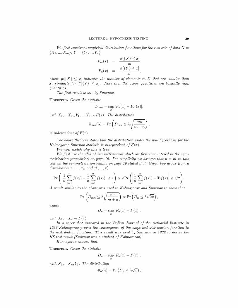
We first construct empirical distribution functions for the two sets of data X =X1, ..., Xm, Y = Y1, ..., Yn
Fm(x) =#[X ≤ x]
m
Fn(x) =#[Y ≤ x]
n,
where #[X ≤ x] indicates the number of elements in X that are smaller thanx, similarly for #[Y ≤ x]. Note that the above quantities are basically rankquantities.
The first result is one by Smirnov.
Theorem. Given the statistic
Dmn = supx
|Fn(x) − Fm(x)|,
with X1, ...Xm, Y1, ..., Yn ∼ F (x). The distribution
Φmn(λ) = Pr
(
Dmn ≤ λ
√
mn
m + n
)
,
is independent of F (x).
The above theorem states that the distribution under the null hypothesis for theKolmogorov-Smirnov statistic is independent of F (x).
We now sketch why this is true.We first use the idea of symmetrization which we first encountered in the sym-
metrization proposition on page 16. For simplicity we assume that n = m in thiscontext the symmetrization lemma on page 16 stated that: Given two draws from adistribution x1, ..., xn and x′
1, ..., x′n
Pr
(∣
∣
∣
∣
∣
1
n
n∑
i=1
f(xi) −1
n
n∑
i=1
f(x′i)
∣
∣
∣
∣
∣
≥ ε
)
≤ 2 Pr
(∣
∣
∣
∣
∣
1
n
n∑
i=1
f(xi) − IEf(x)
∣
∣
∣
∣
∣
≥ ε/2
)
.
A result similar to the above was used to Kolmogorov and Smirnov to show that
Pr
(
Dmn ≤ λ
√
mn
m + n
)
≈ Pr(
Dn ≤ λ√
2n)
,
where
Dn = supx
|Fn(x) − F (x)|,
with X1, ...Xn ∼ F (x).In a paper that appeared in the Italian Journal of the Actuarial Institute in
1933 Kolmogorov proved the convergence of the empirical distribution function tothe distribution function. This result was used by Smirnov in 1939 to derive theKS test result (Smirnov was a student of Kolmogorov).
Kolmogorov showed that:
Theorem. Given the statistic
Dn = supx
|Fn(x) − F (x)|,
with X1, ...Xn, Y1. The distribution
Φn(λ) = Pr(
Dn ≤ λ√
n)
,
30 S. MUKHERJEE, STATISTICS FOR COMP BIO
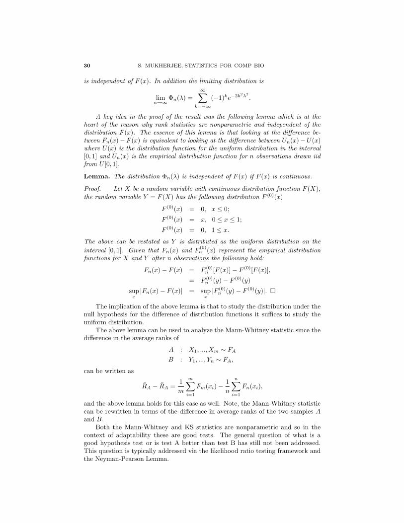
is independent of F (x). In addition the limiting distribution is
limn→∞
Φn(λ) =∞∑
k=−∞(−1)ke−2k2λ2
.
A key idea in the proof of the result was the following lemma which is at theheart of the reason why rank statistics are nonparametric and independent of thedistribution F (x). The essence of this lemma is that looking at the difference be-tween Fn(x)−F (x) is equivalent to looking at the difference between Un(x)−U(x)where U(x) is the distribution function for the uniform distribution in the interval[0, 1] and Un(x) is the empirical distribution function for n observations drawn iidfrom U [0, 1].
Lemma. The distribution Φn(λ) is independent of F (x) if F (x) is continuous.
Proof. Let X be a random variable with continuous distribution function F (X),the random variable Y = F (X) has the following distribution F (0)(x)
F (0)(x) = 0, x ≤ 0;
F (0)(x) = x, 0 ≤ x ≤ 1;
F (0)(x) = 0, 1 ≤ x.
The above can be restated as Y is distributed as the uniform distribution on the
interval [0, 1]. Given that Fn(x) and F(0)n (x) represent the empirical distribution
functions for X and Y after n observations the following hold:
Fn(x) − F (x) = F (0)n [F (x)] − F (0)[F (x)],
= F (0)n (y) − F (0)(y)
supx
|Fn(x) − F (x)| = supx
|F (0)n (y) − F (0)(y)|.
The implication of the above lemma is that to study the distribution under thenull hypothesis for the difference of distribution functions it suffices to study theuniform distribution.
The above lemma can be used to analyze the Mann-Whitney statistic since thedifference in the average ranks of
A : X1, ..., Xm ∼ FA
B : Y1, ..., Yn ∼ FA,
can be written as
RA − RA =1
m
m∑
i=1
Fm(xi) −1
n
n∑
i=1
Fn(xi),
and the above lemma holds for this case as well. Note, the Mann-Whitney statisticcan be rewritten in terms of the difference in average ranks of the two samples Aand B.
Both the Mann-Whitney and KS statistics are nonparametric and so in thecontext of adaptability these are good tests. The general question of what is agood hypothesis test or is test A better than test B has still not been addressed.This question is typically addressed via the likelihood ratio testing framework andthe Neyman-Pearson Lemma.

LECTURE 3. HYPOTHESIS TESTING 31
We start with the case of two simple hypotheses. Again these hypotheses aresimple since the densities are completely specified under the null and alternativehypotheses.
H0 : X ∼ p(X |H0 = T )
HA : X ∼ p(X |HA = T ).
Given the sample X = X1, ..., Xn we can write down the likelihood ratio
Λ =p(X |H0)
p(X |HA).
It would seem reasonable to reject H0 for small values of Λ.
Lemma (Neyman-Pearson). Suppose the likelihood ration test rejects H0 wheneverp(X|H0)p(X|HA) < c has significance level α
Pr
(
p(X |H0)
p(X |HA)< c
)
= α.
Then any other test which has significance level α∗ ≤ α has power less than or equalto the likelihood ratio test.
This lemma address the issue of optimality for simple hypotheses.
Example. We draw n observations iid from a normal distribution,
X1, ..., Xn ∼ N(µ, σ2).
H0 : µ = µ0
HA : µ = µA.
Λ =p(X |µ0, σ
2)
p(X |µA, σ2)=
exp(−∑ni=1(xi − µ0)
2/2σ2)
exp(−∑ni=1(xi − µA)2/2σ2)
.
log(Λ) =
n∑
i=1
(xi − µ0)2 −
n∑
i=1
(xi − µA)2,
=∑
i
x2i − 2µ0
∑
i
xi + nµ20 −
∑
i
x2i + 2µA
∑
i
xi − nµ2A
= 2nX(µ0 − µA) + nµ2A − nµ2
0.
So we can use a statistic t(X)
t = 2nX(µ0 − µA) + nµ2A − nµ2
0,
as our statistic to reject the null. Under the null hypothesis
X ∼ N
(
µ0,σ2
n
)
,
so for the case where µ0 −µA < 0 the likelihood ratio test is a function of X and issmall when X is small. In addition
Pr(X ≥ x0) = Pr
(
X − µ0
σ/√
n>
x0 − µ0
σ/√
n
)
,

32 S. MUKHERJEE, STATISTICS FOR COMP BIO
so we can solvex0 − µ0
σ/√
n= z(α).
Which is the most powerful test under this model.
The problem with the likelihood ratio test framework is that in general thealternative hypothesis is not simple but composite. A typical situation would be
H0 : X ∼ N(µ0, σ2)
HA : X ∼ N(µ 6= µ0, σ2),
where the distribution under the alternative is not specified but forms a familyof distributions. In this setting likelihood ration tests can be generalized to theconcept of generalized likelihood ration tests which also have optimality conditionsbut these conditions are more subtle and we will not study these conditions.
Given the sample X = X1, ..., Xn drawn from a density p(X |θ) with thehypotheses
H0 : θ ∈ ω0
HA : θ ∈ ωA,
where ω0 ∩ ωA = ∅ and ω0 ∪ ωA = Ω. The generalized likelihood ratio is defined as
Λ∗ =maxθ∈ω0 p(X |H0(θ))
maxθ∈ωA p(X |HA(θ)).
For technical reasons we will work with a slight variation of the above likelihoodration
Λ =maxθ∈ω0 p(X |H0(θ))
maxθ∈Ω p(X |HA(θ)).
Note that Λ = min(Λ∗, 1) so small values of Λ∗ correspond to small values of Λ soin the rejection region using either one is equivalent.
Example. We draw n observations iid from a normal distribution,
X1, ..., Xn ∼ N(µ, σ2).
H0 : µ = µ0
HA : µ 6= µ0.
The generalized likelihood is
Λ =
1(σ
√2π)n
exp(− 12σ2
∑ni=1(xi − µ0)
2)
maxµ1
(σ√
2π)nexp(− 1
2σ2
∑ni=1(xi − µ)2)
,
the denominator is maximized at µ = X. So we can write
−2 logΛ =1
σ2
(
n∑
i=1
(xi − µ0)2 −
n∑
i=1
(xi − X)2
)
= n(X − µ0)2/σ2.
We computed previously that if Xi ∼ N(µ0, σ2) that X ∼ N
(
µ0,σ2
n
)
. The dis-
tribution of the square of a normal random variable is the chi-square distributionso
t =n(X − µ0)
2
σ2∼ χ2
1,
LECTURE 3. HYPOTHESIS TESTING 33
where χ21 is the chi-square distribution with one degree of freedom and we would
reject the null hypothesis when
n(X − µ0)2
σ2> χ2
1(α).
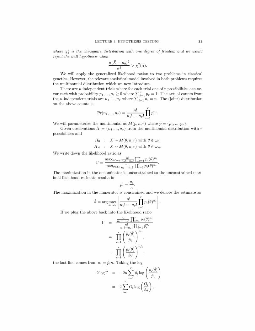
We will apply the generalized likelihood ration to two problems in classicalgenetics. However, the relevant statistical model involved in both problems requiresthe multinomial distribution which we now introduce.
There are n independent trials where for each trial one of r possibilities can oc-cur each with probability p1, ..., pr ≥ 0 where
∑ri=1 pr = 1. The actual counts from
the n independent trials are n1, ..., nr where∑r
i=1 ni = n. The (joint) distributionon the above counts is
Pr(n1, ..., nr) =n!
n1! · · ·nr!
r∏
i=1
pni
i .
We will parameterize the multinomial as M(p, n, r) where p = p1, ..., pr.Given observations X = n1, ..., nr from the multinomial distribution with r
possibilities and
H0 : X ∼ M(θ, n, r) with θ ∈ ω0
HA : X ∼ M(θ, n, r) with θ ∈ ωA.
We write down the likelihood ratio as
Γ =maxθ∈ω0
n!n1!···nr!
∏ri=1 pi(θ)
ni
maxθ∈Ωn!
n1!···nr!
∏ri=1 pi(θ)ni
.
The maximization in the denominator is unconstrained so the unconstrained max-imal likelihood estimate results in
pi =ni
n.
The maximization in the numerator is constrained and we denote the estimate as
θ = argmaxθ∈ω0
[
n!
n1! · · ·nr!
r∏
i=1
pi(θ)ni
]
.
If we plug the above back into the likelihood ratio
Γ =n!
n1!···nr !
∏ri=1 pi(θ)ni
n!n1!···nr!
∏ri=1 pni
i
=
r∏
i=1
(
pi(θ)
pi
)ni
,
=
r∏
i=1
(
pi(θ)
pi
)npi
,
the last line comes from ni = pin. Taking the log
−2 logΓ = −2n
r∑
i=1
pi log
(
pi(θ)
pi
)
= 2
r∑
i=1
Oi log
(
Oi
Ei
)
,
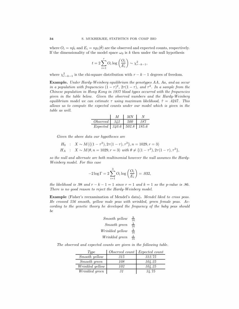
34 S. MUKHERJEE, STATISTICS FOR COMP BIO
where Oi = npi and Ei = npi(θ) are the observed and expected counts, respectively.If the dimensionality of the model space ω0 is k then under the null hypothesis
t = 2
r∑
i=1
Oi log
(
Oi
Ei
)
∼ χ2r−k−1,
where χ2r−k−1 is the chi-square distribution with r − k − 1 degrees of freedom.
Example. Under Hardy-Weinberg equilibrium the genotypes AA, Aa, and aa occurin a population with frequencies (1 − τ)2, 2τ(1 − τ), and τ2. In a sample from theChinese population in Hong Kong in 1937 blood types occurred with the frequenciesgiven in the table below. Given the observed numbers and the Hardy-Weinbergequilibrium model we can estimate τ using maximum likelihood, τ = .4247. Thisallows us to compute the expected counts under our model which is given in thetable as well.
M MN NObserved 342 500 187Expected 340.6 502.8 185.6
Given the above data our hypotheses are
H0 : X ∼ M((1 − τ2), 2τ(1 − τ), τ2, n = 1029, r = 3)
HA : X ∼ M(θ, n = 1029, r = 3) with θ 6= (1 − τ 2), 2τ(1 − τ), τ2,
so the null and alternate are both multinomial however the null assumes the Hardy-Weinberg model. For this case
−2 logΓ = 2
3∑
i=1
Oi log
(
Oi
Ei
)
= .032,
the likelihood is .98 and r − k − 1 = 1 since r = 1 and k = 1 so the p-value is .86.There is no good reason to reject the Hardy-Weinberg model.
Example (Fisher’s reexamination of Mendel’s data). Mendel liked to cross peas.He crossed 556 smooth, yellow male peas with wrinkled, green female peas. Ac-cording to the genetic theory he developed the frequency of the baby peas shouldbe
Smooth yellow 916
Smooth green 316
Wrinkled yellow 316
Wrinkled green 116
The observed and expected counts are given in the following table.
Type Observed count Expected countSmooth yellow 315 312.75Smooth green 108 104.25
Wrinkled yellow 102 104.25Wrinkled green 31 34.75
LECTURE 3. HYPOTHESIS TESTING 35
Given the above data our hypotheses are
H0 : X ∼ M
(
9
16,
3
16,
3
16,
1
16
, n = 556, r = 4
)
HA : X ∼ M(θ, n = 556, r = 4) with θ 6=
9
16,
3
16,
3
16,
1
16
so the null and alternate are both multinomial however the null assumes what becameMendel’s law. For this case
−2 logΓ = 2
4∑
i=1
Oi log
(
Oi
Ei
)
= .618,
the likelihood is .73 and r − k − 1 = 3 since r = 4 and k = 1 so the p-value is .9.There is no good reason to reject the Mendel’s law.
Mendel did this experiment many times and Fisher pooled the results in thefollowing way. Two independent experiments give chi-square statistics with p andr degrees of freedom respectively. Under the null hypothesis that the models werecorrect the sum of the test statistic would follow a chi-square distribution with p+ rdegrees of freedom. So Fisher added the chi-square statistics for all the independentexperiments that Mendel conducted and found a p-value of .99996 !
3.0.12. Multiple hypothesis testing
In the various “omics” the issue of multiple hypothesis testing arises very often.We start with an example to illustrate the problem.
Example. The expression level of 12, 000 genes can be measured with the technologyavailable in one current platform. We measure the expression level of these 12, 000genes for 30 breast cancer patients of which C1 are those with ductal invasion andC2 are those with no ductal invasion. There are 17 patients in C1 and 13 in C2.We consider a matrix xij with i = 1, ..., 12, 000 indexing the genes and j = 1, ..., 30indexing the patients. Assume that for each gene we use a t-test to determine if thatgene is differentially expressed under the two conditions of for each i = 1, ..., 12, 000we assume Xij ∼ N(µ, sigma2)
H0 : µC1
= µC2
HA : µC16= µC2
,
We set the significance level of each gene to α = .01 and we find that we reject thenull hypothesis for 250 genes. At this point we need to stop and ask ourselves abasic question.
Assume H0 is true for i = 1, ..., m = 12, 000 and we observe n = 30 observationsthat are N(µ, σ2) split into groups of 13 and 17. We can ask about the distributionof the following two random variables
ξ = # rejects at α = .01 | H0 = T ∀i = 1, ...m
ξ = # times t ≥ tdf (.01) | H0 = T ∀i = 1, ...m
where tdf is the t-distribution with degree of freedom df . We can also ask whetherIEξ ≈ 120 or IEξ 120. This is the question addressed by multiple hypothesistesting correction.

36 S. MUKHERJEE, STATISTICS FOR COMP BIO
The following contingency table of outcomes will be used ad nauseum in un-derstanding multiple hypothesis testing.
Accept null Reject null TotalNull true U V m0
Alternative true T S m1
W R m
The main quantity that is controlled or worried about in multiple hypothesistesting is V the number of false positives or false discoveries. The other possibleerror is the type II error or the number of false negatives or missed discoveries. Thetwo main ideas are the Family-wise error rate (FWER) and the False DiscoveryRate (FDR). We start with the FWER.
3.0.12.1. FWER. The family-wise error rate consists of finding a cutoff level or αvalue for the individual hypothesis tests such that we can control
αF W ER
= Pr(V ≥ 1),
this means we control the probability of obtaining any false positives. Our objectivewill be to find an α-level or cutoff for the test statistic of the individual tests suchthat we can control α
F W ER.
The simplest correction to control for the FWER is called the Bonferroni cor-rection. We derive this correction
αF W ER = Pr(V ≥ 1),
= Pr (T1 > c ∪ T2 > c, ...,∪Tm > c|H0)
≤m∑
i=1
Pr (Ti > c)
≤ m Pr (T > c)≤ mα,
so if we want to control αF W ER
at for example at .05 we can find a cutoff or select forα = .05
m for the individual hypotheses. There is a huge problem with this correctionthe inequality between steps 2 and 3 can be large if the hypothesis are not disjoint(or the union bound sometimes sucks).
Let us make this concrete by using the example from the beginning of thissection.
Example. In the previous example we use a t-test to determine if a gene is dif-ferentially expressed under the two conditions, for each i = 1, ..., 12, 000 we assumeXij ∼ N(µ, sigma2)
H0 : µC1
= µC2
HA : µC1
6= µC2
,
We set the significance level of each gene to α = .01 this gives us the Bonferronicorrection of α
F W ER= .01 × 12, 000 = 120, which is a joke. In addition, the
assumption that the hypotheses, genes, are independent is ludicrous.
We now use an alternative approach based upon a computational approachthat falls under the class of permutation procedures. This lets us avoid the union

LECTURE 3. HYPOTHESIS TESTING 37
bound and control the FWER more accurately. We will also deal with the issuethat t-distribution assumes normality and our data may not be normal. We willdevelop this procedure in the context of the previous example.
Example. We will use a t-statistic to determine if a gene is differentially expressedunder the two conditions. However, for each j = 1, ..., 12, 000 we do not makedistributional assumptions about the two distributions
H0 : C1 and C2 are exchangeable
HA : C1 and C2 are not exchangeable,
by exchangeable we mean loosely Pr(x, y|y ∈ C1) = Pr(x, y|y ∈ C2).For each gene we can compute the t-statistic: ti. We then repeat the following
procedure π = 1, ..., Π times for each gene
(1) permute labels(2) compute tπi .
For each gene i we can get a p-value by looking at where ti falls in the ecdf generatedfrom the sequence tπi Π
i=1,
pi = Pr(ξ > ti|tπi Ππ=1).
The above procedure gives us a p-value for the individual genes without an assump-tion of normality but how does it help regarding the FWER.
The following observation provides us with the key idea
αF W ER
= Pr(V ≥ 1),
= Pr (T1 > c ∪ T2 > c, ...,∪Tm > c|H0)
= Pr
(
maxi=1,...,m
Ti > c|H0
)
.
This suggests the following permutation procedure For each gene we can com-pute the t-statistic: tim
i=1, where m = 12, 000. Then repeat the following procedureπ = 1, ..., Π
(1) permute labels(2) compute tπi for each gene(3) compute tπ = maxi=1,...,m tπi ,
for each gene we can compute the FWER as
pi,F W ER = Pr(ξ > ti|tπΠπ=1).
One very important aspect of the permutation procedure is we did not assumethat the genes were independent and in some sense modeled the dependencies.
For many problems even this approach with a more accurate estimation of theFWER p-value does not give us significant hypotheses because the quantity we aretrying to control Pr(V ≥ 1) is too stringent.
3.0.12.2. FDR. The false discovery rate consists of finding a cutoff level or α valuefor the individual hypothesis tests such that we can control
qF DR
= IE
[
V
R
]
,
38 S. MUKHERJEE, STATISTICS FOR COMP BIO
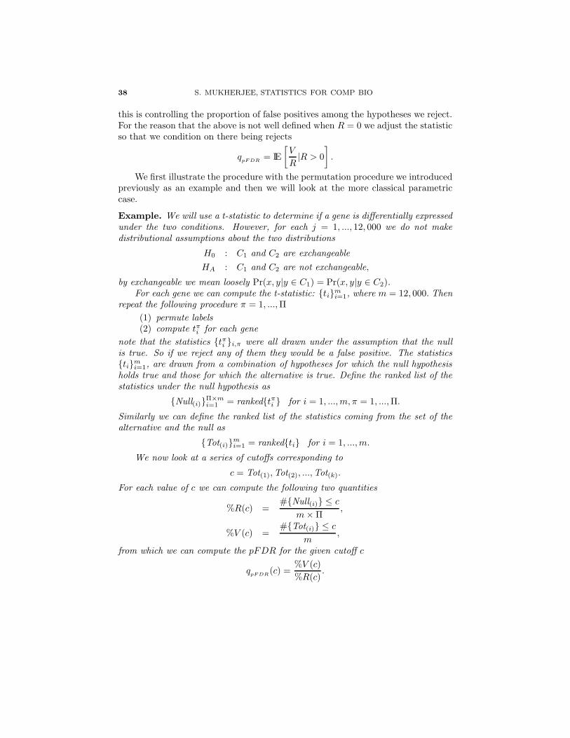
this is controlling the proportion of false positives among the hypotheses we reject.For the reason that the above is not well defined when R = 0 we adjust the statisticso that we condition on there being rejects
qpF DR
= IE
[
V
R|R > 0
]
.
We first illustrate the procedure with the permutation procedure we introducedpreviously as an example and then we will look at the more classical parametriccase.
Example. We will use a t-statistic to determine if a gene is differentially expressedunder the two conditions. However, for each j = 1, ..., 12, 000 we do not makedistributional assumptions about the two distributions
H0 : C1 and C2 are exchangeable
HA : C1 and C2 are not exchangeable,
by exchangeable we mean loosely Pr(x, y|y ∈ C1) = Pr(x, y|y ∈ C2).For each gene we can compute the t-statistic: tim
i=1, where m = 12, 000. Thenrepeat the following procedure π = 1, ..., Π
(1) permute labels(2) compute tπi for each gene
note that the statistics tπi i,π were all drawn under the assumption that the nullis true. So if we reject any of them they would be a false positive. The statisticstim
i=1, are drawn from a combination of hypotheses for which the null hypothesisholds true and those for which the alternative is true. Define the ranked list of thestatistics under the null hypothesis as
Null(i)Π×mi=1 = rankedtπi for i = 1, ..., m, π = 1, ..., Π.
Similarly we can define the ranked list of the statistics coming from the set of thealternative and the null as
Tot(i)mi=1 = rankedti for i = 1, ..., m.
We now look at a series of cutoffs corresponding to
c = Tot(1),Tot(2), ...,Tot(k).
For each value of c we can compute the following two quantities
%R(c) =#Null(i) ≤ c
m × Π,
%V (c) =#Tot(i) ≤ c
m,
from which we can compute the pFDR for the given cutoff c
qpF DR(c) =%V (c)
%R(c).


