
TEMPERATURE PREDICTION IN HOT TAPPING PROCESS FOR HIGH
PRESSURE PIPELINE
MUHAMMAD AIZADT BIN ROSMAN
MECHANICAL ENGINEERING
UNIVERSITI TEKNOLOGI PETRONAS
JANUARY 2017


i
Temperature Prediction in Hot Tapping Process for High Pressure Pipeline
by
Muhammad Aizadt bin Rosman
18334
Dissertation submitted in partial fulfillment of
as a requirement for the
Bachelor of Engineering (Hons)
(Mechanical)
JANUARY 2017
Universiti Teknologi PETRONAS
Bandar Seri Iskandar
32610 Seri Iskandar
Perak Darul Ridzuan
Malaysia
ii
CERTIFICATION OF APPROVAL
Temperature Prediction in Hot Tapping Process for High Pressure Pipeline
by
Muhammad Aizadt bin Rosman
18334
A project dissertation submitted to the
Mechanical Engineering Department
Universiti Teknologi PETRONAS
In partial fulfillment of the requirement for the
BACHELOR OF ENGINEERING (Hons)
(MECHANICAL)
Approved by,
___________________
(Dr William Pao King Soon)
Universiti Teknologi PETRONAS
Bandar Seri Iskandar, Perak
January 2017

iii
CERTIFICATE OF ORIGINALITY
This is to certify that I am responsible for the work submitted in this project that the
original work is my own except as specified in the references and acknowledgements, and
that the original work contained herein have not been undertake or done by unspecified
sources or persons.
_____________________
MUHAMMAD AIZADT BIN ROSMAN

iv
ABSTRACT
Welding onto an in-service pipeline during hot tapping process are extremely risky and require
thorough preparation and precautions, where the probability of occurrence of occupational hazards
and injuries are high. Since the increase in surrounding temperature inside the working system are
unpredictable, the internal pipe wall temperature and the process fluid temperature inside the pipe
are unknown during operation.
Therefore, this project is conducted to i) predict inner pipe wall temperature and ii) to estimate
temperature of the process fluid inside the pipeline during in-service welding and iii) to construct
relevant methodology and reference chart in predicting internal fluid temperature by using existing
information from wall temperature chart provided by PTS 31.38.60.10 “Hot-Tapping on Pipelines,
Piping and Equipment”.
These objectives will be achieved by conducting thermal Computational Fluid Dynamics (CFD)
simulations on 2D heat transfer model on a pipe’s cross-sectional plane by using ANSYS
Mechanical APDL. The thermal CFD simulations for this project are divided into two phases. In
the first phase of this project, CFD simulations are conducted without the introduction of process
fluid. The data obtained will be used to compare with the information gathered from existing PTS
chart for the purpose of CFD model validation. Then, the second phase of the project is conducted
by introducing process fluid inside the validated 2D model. All of the temperature data obtained
will be used to construct a new temperature prediction chart for hot-tapping process which include
the process fluid parameter.
At the end of this project, it is expected that the proposed temperature prediction chart will be able
to assist field engineers and operators in estimating the temperature of critical locations inside the
working system and establishing a safe permissible temperature range to safely conduct in-service
welding to avoid explosion and burn through risk.

v
ACKNOWLEDGEMENT
Greatest gratitude to The Most Gracious and The Most Merciful for His countless mercy and
enlightenment in completing the first half of my Final Year Project Programme. Thanks foremost
to my family especially to my dearest mother on whom I always admire for her true grit in raising
me up as a single mother through every hardships that we have encountered in life so far.
I would like to express my thanks to the Onshore Gas Terminal communities for introducing and
exposing myself to the oil and gas engineering world during my internship programme under
PETRONAS Carigali Sdn. Bhd. in Kerteh, Terengganu. The experiences that I have gained during
the internship have effectively prepare myself at least some knowledge on the oil and gas
operations such as in hot tapping operations to help me proceed with this project.
Special appreciation goes to Dr. William Pao for his useful guidance and coaching in developing
this project. Throughout the weekly meeting sessions, I have truly learnt a lot in terms of
conducting formal research methodologies, documentations and developing soft skills in this
once-a-life experience. Throughout the discussions with him, I was exposed to reality of
engineering and business world that we live in, inspiring myself to become a better person in every
aspects to be ready face the real world challenges.
I also would like to extend my gratitude towards my supportive friends for their psychological and
moral support in developing my project. Last but not least, I would like to thank those who
indirectly, have contributed in giving me guidance and opinions in developing this project, hence
making the moment of doing this Final Year project to a moment to remember in my life.
vi
TABLE OF CONTENTS
ABSTRACT ..................................................................................................................................iv
ACKNOWLEDGEMENT ............................................................................................................ v
TABLE OF CONTENTS ............................................................................................................vi
LIST OF FIGURES ................................................................................................................... vii
LIST OF TABLES .................................................................................................................... viii
CHAPTER 1: INTRODUCTION ................................................................................................ 1
1.1 Background of Study ...................................................................................................... 1
1.2 Problem Statement .......................................................................................................... 2
1.3 Project Objectives ........................................................................................................... 3
1.4 Scopes of Study ............................................................................................................... 3
1.5 Project Relevancy ........................................................................................................... 4
1.6 Project Feasibility ........................................................................................................... 5
CHAPTER 2: LITERATURE REVIEW .................................................................................... 6
2.1 Critical Analysis .............................................................................................................. 6
CHAPTER 3: RESEARCH METHODOLOGY ..................................................................... 17
3.1 Research Methodology ................................................................................................. 17
3.2 Key Milestone ............................................................................................................... 18
3.3 Project Gantt Chart ....................................................................................................... 19
3.4 Softwares Utilized ......................................................................................................... 20
3.5 Preliminary Calculations ............................................................................................... 21
3.6 Preparation of ANSYS Simulation ............................................................................... 28
CHAPTER 4: RESULTS AND DISCUSSIONS ...................................................................... 32
4.1 ANSYS Simulation Stage I: Prediction of Inner Pipe Wall Temperature .................... 32
4.2 ANSYS Simulation Stage II: Prediction of Process Fluid Temperature ....................... 36
CHAPTER 5: CONCLUSION AND RECOMMENDATION ............................................... 40
5.1 Conclusion .......................................................................................................................... 40
5.2 Recommendation ................................................................................................................ 40
REFERENCES ............................................................................................................................ 42

vii
LIST OF FIGURES
Figure 2.1: Typical hot tap machine setup ..................................................................................... 6
Figure 2.2: Hot tapping procedures................................................................................................ 7
Figure 2.3: Reduced branch fitting ................................................................................................ 8
Figure 2.4: Reinforced set-on branch ............................................................................................. 8
Figure 2.5: Preformed split tee ....................................................................................................... 8
Figure 2.6: Gaussian heat source distribution model ................................................................... 11
Figure 2.7: Double ellipsoidal heat source (DEHS) model developed by Goldak and Akhlagi .. 12
Figure 2.8: Appendix 2 “Welding Temperature of Pipe Wall – Initial Temperature of 25°C” ... 13
Figure 2.9: Appendix 3 “Welding Temperature of Pipe Wall – Initial Temperature of 150°C” . 14
Figure 3.1: Project methodology flowchart ................................................................................. 17
Figure 3.2: Project key milestone ................................................................................................ 18
Figure 3.3: ASME/ANSI B36.10 "Welded and Seamless Steel Pipe" on schedule 30 standard . 21
Figure 3.4: Appendix 2 “Welding Temperature of Pipe Wall – Initial temperature of 25°C” .... 24
Figure 3.5: Visualization of problem as 2D heat transfer finite element model .......................... 28
Figure 3.6: Defining the geometries of the 2D heat transfer finite element model ...................... 29
Figure 3.7: Developed ANSYS 2D finite element model (without fluid introduction) ............... 31
Figure 4.1: Temperature profile showing maximum pipe wall and inner pipe wall temperature 32
Figure 4.2: Estimated inner pipe wall temperature from PTS chart at the same condition .......... 33
Figure 4.3: Improved heat source modelling on ANSYS 2D model ........................................... 33
Figure 4.4: Graph of estimated pipe wall temperature vs. pipe wall thickness ............................ 35
Figure 4.5: Temperature profile with the introduction of process fluid inside the system .......... 36
Figure 4.6: Locations of maximum process fluid temperature .................................................... 37
Figure 4.7: Graph of estimated process fluid temperature vs. pipe wall thickness ...................... 38

viii
LIST OF TABLES
Table 3.1: Softwares required for this project .............................................................................. 20
Table 3.2: Welding procedure table extracted from Welding Procedures Specifications............ 23
Table 3.3: Pipe temperature derating factor obtained from PTS 31.38.60.10 .............................. 25
Table 3.4: Table A-1: Basic allowable stresses in tension for metals from ASME B13.3 .......... 26
Table 3.5: Physical properties of natural gas condensate in OGT ............................................... 30
Table 3.6: Physical properties of API 5L Grade B Carbon Steel ................................................. 30
Table 3.7: Convection properties of air ....................................................................................... 31
Table 4.1: Comparison of pipe wall temperature from PTS Chart with ANSYS simulation ...... 34
Table 4.2: Inner pipe wall temperatures from ANSYS simulations for different heat input ....... 34
Table 4.3: Estimated fluid temperatures from ANSYS simulations for different heat input ....... 37

1
CHAPTER 1: INTRODUCTION
1.1 Background of Study
Welding onto in-service pipeline in hot tapping process are usually required in order to facilitate
repair and modifications to an existing pipeline, such as to install a branch connection to the main
pipeline in a process plant without having shutdown. However, welding onto in-service pipeline
is a high risk activity where strict precautions and engineering considerations must be taken at all
times during performing the activity. The most common risks encountered are leaking and
explosion by weld burn-through, chemical reaction due to system instability and increased
susceptibility of pipe wall material to hydrogen induced cracking that can result in loss of
structure’s strength.
According to Sabapathy et al. (2005), one the factors that make in-service welding
difficult is the characteristics of internal flow of process fluid (gas or liquid) inside the pipeline
which create large heat losses across the pipe wall during welding. This results in fast weld cooling
rates where the welds will most likely to have hard heat affected zones (HAZ) and decreased in
HAZ toughness through formation of hardened areas. This situation will increase their possibility
and susceptibility to hydrogen induced cracking (HIC). The second problem addressed by
Sabapathy et al. (2005) is the loss of mechanical strength due to high temperature rise during
welding. The loss of mechanical strength will create the possibilities of localized rupture in the
pipe wall structure due to high internal process fluid pressure. The third factor is the violent
interaction between the fluid and the inner pipe wall surface in high temperature environment
which can lead to explosion as addressed in API 577 “Welding Inspection and Metallurgy”.
Current studies by EWI/BMI (Edison Welding Institute and Battelle Memorial Institute)
provides a numerical 2D finite difference model to simulate welding and hot tapping onto in-
service pipelines that allows the prediction of inner pipe wall surface temperature and the weld
cooling time for given set of boundary conditions. This model evaluates the risk of penetration
(burn-through) and limits the risk of hydrogen cracking in the HAZ region during welding process.
Meanwhile, Goldak et al. (1992) and Sabapathy et al. (2005) used a 3D finite element model to
calculate the thermal fields for circumferential fillet welds of direct branching. Their research
finding shows that the shape and the weld bead size have strong influence on the calculated depth
of weld penetration and temperature profile around the weld pool.

2
However, there is a lack of study in terms of prediction of process fluid temperature inside
a pipeline during in-service welding. Therefore, the main purposes of this project are to predict
the inner surface temperature of pipe wall during welding as well as the temperature of the
process fluid inside the pipeline for given set of boundary conditions. In order to achieve the
target, this paper will construct relevant methodology and a reference chart to predict the fluid
temperature by using existing information from wall temperature chart provided by PTS
31.38.60.10 “Hot-Tapping on Pipelines, Piping and Equipment”.
1.2 Problem Statement
The most common risks related to welding onto an in-service pipeline during hot tapping process
is the unpredictable increased surrounding temperature inside the system. During in-service
welding, the internal pipe wall temperature and the process fluid temperature inside the pipe
are unknown. This situation might possibly lead to serious occurrence of occupational hazards
and structure failures such the formation of hydrogen induced cracking (HIC) inside pipe wall
structure, weld burn-through and violent chemical reactions between the pipe wall’s surfaces with
the internal fluid flow inside the pipe due to increase in surrounding temperature.
The risk of hydrogen induced cracking at the weld points arise when the cooling rate and
heat loss from molten weld pool is accelerated due to high flow rate of process fluid flowing inside
pipeline. As a result, the weld heat are removed away from the pipe wall material in short amount
of time, resulting in fast weld cooling rate. Apart from fluid’s flow rate, this phenomena are
dependent on various fluid flow characteristics such as type of fluid, density, viscosity, velocity,
hydrostatic and dynamic pressure, thermal conductivity, heat transfer coefficients and more.
Pipe’s geometrical, physical, mechanical, and metallurgical properties also contribute to this
phenomena. Moreover, fast weld cooling rate will decrease the HAZ toughness at the weld points,
which in turns reduce the pipe’s mechanical strength. This situation might lead to localized rupture
at weld points due to high internal pressure acting along the radial direction of a pipeline. Another
common issue is the risk of burn-through, where depth of penetration of molten weld pool become
more significant as the temperature of the weld pool is raised. Here, the thermochemical
interaction between the fluids with the increasing temperature of the inner surface of the pipe (i.e.
due to fluid’s flammability) can be violent, and might lead to sudden explosion in the pipe.

3
Therefore, it is very important to determine related in-service welding risks during hot
tapping process by predicting the inner surface temperature of the pipe wall as well as the
internal fluid temperature inside pipeline.
1.3 Project Objectives
The objectives of this project are:
To predict inner surface temperature of pipe wall during in-service welding.
To predict fluid temperature inside the pipeline during in-service welding.
To construct relevant methodology and reference chart to predict the fluid temperature
by using existing information from wall temperature chart provided by PTS 31.38.60.10
“Hot-Tapping on Pipelines, Piping and Equipment”.
1.4 Scopes of Study
The scopes of study of this project are narrowed down to:
Heat source distribution model is based on only heat input from welding activity,
neglecting other external heat sources from surroundings such as heat from ambient
environment.
The influence of existing thermal stresses (due to improper heat treatment during pipe’s
fabrication process) or mechanical stresses (due to internal acting pipe pressure) are
neglected.
Heat source distribution model only consider heat transfer process along the radial
direction of the pipeline on the cross-sectional plane of a pipe, while heat transfer process
along the longitudinal direction of the pipeline is not considered.
The analysis only consider heat input from first layer of weld, without considering
multilayer welding (multi pass welding).
Heat source distribution is assumed to be static and does not change in amount and
direction with time. Thus, the analysis is steady state.
2D finite element model is constructed for the purpose of model development, simulation
and evaluation.

4
The process fluid level tested in simulations are assumed to be half-filled and assumed to
be static throughout the simulations.
The simulations are done with pipe thickness with more than 5 mm since the application
of welding service for pipe wall thickness below 5mm is restricted according API 2201
“Procedures for Welding or Hot Tapping on Equipment in Service” due to high burn-
through risk.
1.5 Project Relevancy
This project is expected to be beneficial to the industry especially to oil and gas society by
providing significant output to aid the engineers, project managers and related workforces in
performing safe hot tapping operations inside a plant. As a consequent, this study is significant as
a means of preventative measures where hot tapping operations might mostly result in serious
hazards and dangerous incidents such as explosion even if all the precautions are taken. This is
due to lack of study in terms controlling the working temperature changes, especially when dealing
with applications of flammable fluids at high temperature.
The output of this project, which is the construction of relevant methodology to evaluate
surrounding system temperature changes during in-service welding in hot tapping operations will
help the engineers to predict the internal temperature of the pipe wall, as well as the temperature
of the fluid flowing inside the pipeline. From this information, the engineers can determine and
develop safe working limit of their operations by controlling critical operational variables such as
welding heat input and dynamic process fluid characteristics to avoid the possibilities of
occupational hazards and risks especially leak and explosion hazard. A reference chart which is to
be constructed from this project methodology based on existing wall temperature chart provided
by PTS 31.38.60.10 “Hot-Tapping on Pipelines, Piping and Equipment” is expected to be reliable
and useful for the engineers, while at the same time should be easy to use and yield accurate
prediction. Therefore, the output of this project is expected to be relevant in the real world: to ease
the operations of hot tapping in various applications while preventing any occurrence of
occupational hazards.

5
1.6 Project Feasibility
This project is expected to be feasible within the planned time frame starting from project planning,
project execution, project documentation and concluded with project presentation.
In terms of experience and exposure in developing the project methodology, this project
still require the aid of specialized engineers and supervisors since some criteria and variable might
be overlooked by the project executor which may result in developing incorrect methodology and
output. With the aids of specialized personnel, the accuracy of the project methodology should
become accurate and feasible to be implemented in real world. The feasibility study concluded
that this project should be able to be implemented in real engineering application, specifically in
hot tapping operations to produce safe working environment for all participated personnel in the
operation.
6
CHAPTER 2: LITERATURE REVIEW
2.1 Critical Analysis
2.1.1 Hot Tapping
Hot tapping process refers to the installation of connections to pipelines while they remain in
service. Compared to cold cut, hot tapping doesn’t require the need of plant process shutdown and
pipeline depressurization which usually may results in loss of revenue due to loss of pipelines’
throughput and gases to atmosphere. Hot tapping are performed in order to repair pipe areas that
experience mechanical damage, corrosion, erosion, or for modification purposes. The
modification purposes of pipelines may be related to installation of branches for flow modification
or for instrumentation installations. Hot tapping process involves high risk welding activities,
which are performed onto in-service pipelines. Therefore, proper risk assessment must be carefully
examined to ensure the safety of welding operations to both handling personnel and to the
equipment themselves. A successful hot tap operation will minimize the operational effect and
results in no spills or fluid emission out of the live system. Hot tapping is commonly practices in
oil and gas industry where the economic and time factor are the upmost considerations in process
production and distribution.
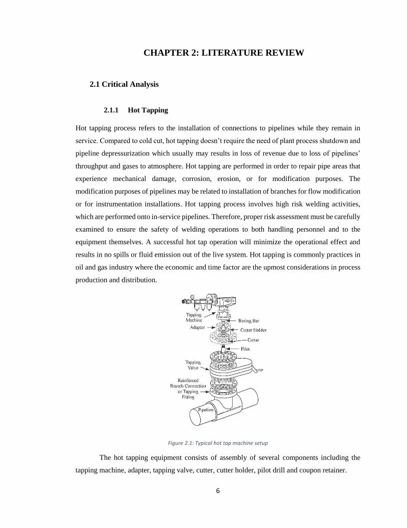
Figure 2.1: Typical hot tap machine setup
The hot tapping equipment consists of assembly of several components including the
tapping machine, adapter, tapping valve, cutter, cutter holder, pilot drill and coupon retainer.

7
Hot tapping process include the following steps: installation of hot tapping machine, drilling and perforation by using hot tap machine (which
is guided by pilot drill), coupon and drill bit retrieval (including gate valve isolations) and machine removal. The illustration below described the
further details of each process involved in hot tapping operation.
Figure 2.2: Hot tapping procedures

8
In hot tapping, the most common type of hot-tap connection used are reduced branch fitting,
reinforced set-on branch and preformed split tee as shown in the figures below:
Figure 2.3: Reduced branch fitting
Figure 2.4: Reinforced set-on branch
Figure 2.5: Preformed split tee

9
2.1.2 Hot Tapping Operating Windows
Based on PETRONAS Technical Standard for “Hot Tapping on Pipelines, Piping and
Equipment” (PTS 31.38.60.10), a decision whether hot tapping process should be performed must
be based on several criteria and operating conditions in order to eliminate and reduce any potential
hazards in terms of human safety, equipment conditions and environmental risks. The criteria are
listed as follows:
Safety of the workplace,
Condition of the pipe or equipment under consideration,
Configuration of the connections,
Code/statutory requirements,
Operating and process conditions,
Technical capabilities of the drilling equipment under the operating conditions
(pressure, temperature, nature of the product),
Related welding problems,
Economic aspects,
Environmental/pollution aspects.
2.1.3 Hot Tapping Risks
When dealing with welding onto in-service pipeline for hot tapping process, there are
three common risks: leaking and explosion via burn-through, thermochemical reaction inside
pipeline due to chemical instability at high temperatures and hydrogen induced cracking (HIC)
at the weld locations. According to Sabapathy (2005), hydrogen induced cracking (HIC) in high
strength steels are particularly caused by the flow of fluid (liquid or gas) inside the pipelines which
tend to cause a large heat loss in the pipe wall, resulting in fast weld cooling. During fast weld
cooling of molten weld pool area at the heat affected zone (HAZ) of the base metal, the
metallurgical and chemical properties in that areas are altered. This cause material’s sensitization,
cracking and reduction of material’s resistance towards corrosion. Toughness of HAZ will
decrease through formation of hard microstructures and creep which are brittle and hard at the
affected region (Lima, 2014). Metallurgical changes also can lead to the formation of nitrides at
the HAZ, which can affect the weldability making the process of welding more difficult. The
factors that influence the characteristics of HAZ at the weld locations include the properties of
10
base material, properties of weld filler materials for non-autogenous welding processes, and the
concentration of heat input during welding.
In most application, weld personnel and engineers will usually increase the heat input to
reduce significant heat loss into the flowing process fluid in order to deal with high cooling rate
issues during in-service welding. However, it should be noted that this action can cause loss of
mechanical strength in pipe’s material due to significant temperature rise in the system. As a
consequent, high local stresses in or near the HAZ are formed during welding. This situation will
directly induce localized rupture of the pipe wall due to high radial forces coming from internal
fluid pressure when the weld heat input is increased (Lima, 2014). The depth of weld penetration
and risk of pipe wall burn-through are also increased. However, the research conducted by
Tahami and Asl (2009) stated that localized rupture may occur even with partial penetration from
welding by considering the effect of internal pressure added with existing thermal stresses in the
pipe wall. Therefore, in practical application as addressed in API 2201 “Procedures for Welding
or Hot Tapping on Equipment in Service’’, welding process for pipe wall with thickness below
5mm are strictly restricted to avoid risk of burn-through due to high heat input generated from
welding processes. Based on the study conducted by Lima (2005), he limits the weld temperature
to be 980°C for low hydrogen electrodes and 760°C for cellulosic electrodes to avoid the risk of
penetration.
Hydrogen induced cracking which occurs when ambient hydrogen permeate into the
pipe wall during welding at high temperatures can be diffused from the welded area by conducting
post weld heat treatment (PWHT). This process is known as post heating where the material
needs to be heated to a certain temperature for a number of hours and gradually cooled, depends
on the thickness and properties of the materials involved. Usually, materials with higher carbon
content or carbon equivalent (CE) are more likely required to undergo PWHT. This is very
important consideration since the high-strength low-alloy steel (HSLA) material for most pipe
application involved for hot tapping process have significant amount of CE to suit for weldability.
Post weld heat treatment should be conducted immediately after the weld process is completed
rather than allowing the weld to eventually cool. This will prevent significant heat loss into
surrounding environment, especially into the process fluid. At the same time, this heat treatment
serves to relieve the residual stress formed due to increase in temperature during welding, out of
the system.
In addition to the risks of welding onto in-service pipelines, Lima (2014) considered a
third factor which is the interaction between the process fluid and the temperature on the

11
inner surface of the pipe when the temperature of the system is raised significantly during
welding process. He furthermore addressed that internal explosion might occur due to instable
thermochemical reaction as most process product involved in hot tapping for oil and gas
applications are flammable and has low flash point. This findings are consistent with the statement
addressed in API 577 “Welding Inspection and Metallurgy”.
2.1.4 Existing Methodologies Developed Related to Hot Tapping Problems
To cope with the hot tapping related risks, numerical simulation of welding service has
been demonstrated by the work of EWI/BMI (Edison Welding Institute/Battelle Memorial
Institute) to predict the inner surface temperature of the pipe and the cooling time for the
molten weld to solidify (ΔT800-500), for given set of welding parameters, pipe geometry and
properties, along with the coefficient of heat transfer by convection which is obtained empirically
as the function of process fluid flowing inside the pipeline. This is a 2D model finite difference
which simulates the welding gloves of welding activity conducted during hot tapping. Welding
processes are considered as thermal-mechanical-metallurgical coupled processes. Therefore, the
most important boundary condition in BMI/EWI model is the heat source modelling.
During welding, the heat input melts both filler materials added to the base metals creating
a molten pool area. Compared to the traditional punctual and linear welding heat source
assumption, Lima (2014) modelled the heat source from the welding activity by using Gaussian
Heat Source Distribution which is more realistic and accurate to be implemented practically.
Gaussian heat source distribution is a model to describe heat generated distribution over a surface.
Figure 2.6: Gaussian heat source distribution model

12
Research conducted by Goldak et al. and Sabapathy et al. in 1992, found that the shape
and the weld bead size have a strong influence on the calculated depth of penetration and
temperature profile around the molten weld pool. They have used a 3D finite element model
to calculate the thermal fields for circumferential filet welds of direct branching. According to
Sabapathy et al. (1992), the use of empirical relations between the welding parameters and the
size and shape of the weld bead is an appropriate way to define the geometry of the weld pool and
the coordinate of the heat sources. Sabapathy et al. and Goldak et al. also develop an equation to
characterize the heat distribution by non-autogenous welding sources which is the Double
Ellipsoidal Heat Source (DEHS) model which defines the heat flow Q (kJ/mm3). The model is
further described the equation and figure below.
𝑞(𝑥, 𝑦, 𝜉, 𝑡) =6𝑓√3𝑄
𝑎𝑏𝑐𝜋√𝜋𝑒
−3𝑥2
𝑎2 𝑒−3𝑦2
𝑏2 𝑒−3𝑧2
𝑐2 … (1)
Figure 2.7: Double ellipsoidal heat source (DEHS) model developed by Goldak and Akhlagi
This equation considers the factors of amount of heat input, pipe’s thickness, weld speed,
voltage, arc efficiency, type of welding processes to estimate the size and shape (geometries) of
molten weld pool in terms of width, depth, and length which are represented by symbols: a, b and
c respectively. This allow the analysis on burn-through prediction to avoid the risk of penetration
in welding onto in-service pipelines.
2.1.5 Engineering Concepts Related to Hot Tapping Processes
This section described the common engineering principles and formulations related to
problem solving of hot-tapping operations.
Calculation of Maximum Temperature of the Wall
𝐻𝐼 = 𝐾 (𝑉. 𝐴
𝑆) … (2)

13
Where:
HI = Heat input (J/mm)
K = Net factor (0.85 for butt weld, 0.57 for fillet welds)
V = Voltage (V)
A = Current (A)
S = Welding travel speed (mm/s)
*The permitted ranges of voltage, current and welding speed are obtained from PTS 30.10.60.30
“Welding Procedure Specification”
Estimation of Weld Penetration and Maximum Inner Pipe Wall Temperature from Heat
Input Value According to PTS 30.38.60.10
Figure 2.8: Appendix 2 “Welding Temperature of Pipe Wall – Initial Pipe Wall temperature of 25°C”

14
Figure 2.9: Appendix 3 “Welding Temperature of Pipe Wall – Initial Pipe Wall temperature of 150°C”
Calculation of Pressure of the Process Liquid
𝑃 =2𝑆 ∙ 𝑡 ∙ 𝐹 ∙ 𝐸 ∙ 𝑇
𝐷… (3)
Where:
P = Maximum allowable operating pressure during welding (MPa)
S = Specific minimum yield stress (N/mm2) (for off-plot pipeline)
= Basic allowable stress (N/mm2) (for on-plot piping)
D = Nominal outside diameter of run pipe (mm)
t = Reduced wall thickness (where t = ta – u) (mm)

15
u = Reduction in wall thickness during welding, represent the weld pool penetration (mm)
ta = Minimum actual wall thickness which is determined by ultrasonic measurement (mm)
F = Safety factor or design factor
E = Longitudinal joint factor
T = Temperature of derating factor derived from Table 1
Cooling Rate Estimation for In-Service Welding in Hot-Tapping
𝐻𝑛𝑒𝑡 = 𝑓 (𝑉. 𝐴
𝑆) … (4)
Where:
Hnet = Net heat input (kJ/mm)
f = Net factor or fraction of heat generated and transferred to the plate (0.85 for butt weld,
0.57 for fillet welds)
V = Voltage (V)
A = Current or amperage (A)
S = Welding travel speed (mm/s)
Criteria Checking for Thin-Walled Pipes and Thick-Walled Pipes
To decide which cooling rate equation should be used for cases involving thin-walled pipes and
thick-walled pipes. The determining factors are: number of passes required to complete the
weld and relative plate thickness (τ).
Relative Pipe Thickness Criteria
𝜏 = 𝑡 {𝜌𝐶(𝑇𝑖 − 𝑇𝑜)
𝐻𝑛𝑒𝑡} .
1
2… (5)

16
Where:
t = Plate thickness (mm)
ρ = Density of the pipe material (g/cm3)
C = Specific heat capacity (KCal/°C.g)
Ti = Instantaneous pipe wall temperature or interest pipe wall temperature (°C)
To = Initial pipe wall temperature (°C)
Hnet = Net heat input (kJ/mm)
Apply thin-walled cooling rate equation when: τ < 0.6 and apply thick-walled cooling rate
equation when τ > 0.9. If the value falls between the range of 0.6 to 0.9, 0.75 is used as limit value
and preferable to use thick-walled cooling rate equation.
Cooling Rate Equations for Thin-Walled Pipes and Thick-Walled Pipes
𝐶𝑅𝑡ℎ𝑖𝑛 = {2𝜋𝑘𝜌𝐶 (𝑡
𝐻𝑛𝑒𝑡) (𝑇𝑖 − 𝑇𝑜)3}℃/ sec … (6)
𝐶𝑅𝑡ℎ𝑖𝑐𝑘 = {(2𝜋𝑘(𝑇𝑖 − 𝑇𝑜))/𝐻𝑛𝑒𝑡}℃/ sec … (7)
Where:
t = Plate thickness (mm)
k = Thermal conductivity pipe material
ρ = Density of the pipe material (g/cm3)
C = Specific heat capacity (KCal/°C.g)
Ti = Instantaneous pipe wall temperature or interest pipe wall temperature (°C)
To = Initial pipe wall temperature (°C)

17
CHAPTER 3: RESEARCH METHODOLOGY
3.1 Research Methodology
The methodology of this project are outlined in the flowchart below:
Start
Problem Identification &Literature Review
Development of New Methodology Based on Information Gathered from PTS Standard
ANSYS Simulation Stage I: Development of Proper Simulation Model to Predict Pipe Wall
Temperature
Results Validation: Simulation Results vs. Value from PTS Chart
ANSYS Simulation Stage II: Development of Advanced Simulation Model to Predict
Internal Fluid Temperature
Construction of a Reference Chart based on Information Gathered from Project
Simulations
valid
invalid
End
Project Documentation
Figure 3.1: Project methodology flowchart
FYP I
FYP II

18
3.2 Key Milestone
12 Sep. 16 17 May. 1701/10/2016 01/11/2016 01/12/2016 01/01/2017 01/02/2017 01/03/2017 01/04/2017 01/05/2017
12/09/2016
Project Start: Topic Selection and
Problem Identification
17/05/2017
Project End: Final Report Documentation
and Project Presentation
15/11/2016
Development of Finite Element Simulation
Model #1 by Using ANSYS Workbench Thermal
Transient. Objective: To Determine the Internal
Pipe Wall Temperature
20/12/2016
Preliminary Results and
Interim Report Documentation
16/01/2017
Development of Advanced Finite Element
Simulation Model #2 by Using ANSYS Workbench
Thermal Transient. Objective: To Determine
the Internal Process Fluid Temperature
20/03/2017
Construction of a Reference Chart Based on
Information Gathered from Simulations
30/12/2016 - 16/01/2017
SEMESTER BREAK
12/09/2016 - 30/12/2016
FYP I16/01/2017 - 17/05/2017
FYP II
Figure 3.2: Project key milestone

19
3.3 Project Gantt Chart

20
3.4 Softwares Utilized
This project mainly utilize the application of softwares to develop desired project objectives and
results. The related softwares used in this project are listed in the tables below.
Table 3.1: Softwares required for this project
SOFTWARES FUNCTIONS AND APPLICATIONS
Microsoft Word 2013 As a project documentation platform, mainly emphasizes on report
writing.
Microsoft Excel 2013 As a data analysis platform: to construct project tables, graphs and
charts from data extracted from simulations.
Microsoft PowerPoint 2013 As a project documentation platform, for project presentation.
Microsoft Visio 2013 As a project documentation platform: to construct project charts,
2D model drawings
Solid Edge V19 (Draft) As a project documentation platform: to construct 2D model
drawings with proper dimensioning.
ANSYS V15 Mechanical
Workbench
As a project simulation platform where 2D finite element models
are constructed. Simulations are done based on user defined
specific process boundary conditions. This software allow for
thermal transient analysis of 2D model including the development
of temperature profile and nodal analysis of a model. Also acts as
data analysis platform to investigate the real-time simulation
results.
21
3.5 Preliminary Calculations
3.5.1 Numerical Calculations on Process Conditions: Prediction of Inner Pipe
Wall Temperature and Depth of Penetration by Using PTS Reference
Chart
i. Selection of Pipe Material
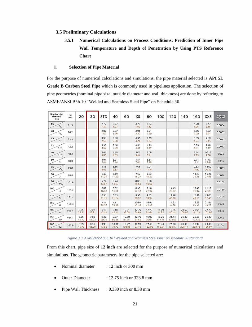
For the purpose of numerical calculations and simulations, the pipe material selected is API 5L
Grade B Carbon Steel Pipe which is commonly used in pipelines application. The selection of
pipe geometries (nominal pipe size, outside diameter and wall thickness) are done by referring to
ASME/ANSI B36.10 “Welded and Seamless Steel Pipe” on Schedule 30.
Figure 3.3: ASME/ANSI B36.10 "Welded and Seamless Steel Pipe" on schedule 30 standard
From this chart, pipe size of 12 inch are selected for the purpose of numerical calculations and
simulations. The geometric parameters for the pipe selected are:
Nominal diameter : 12 inch or 300 mm
Outer Diameter : 12.75 inch or 323.8 mm
Pipe Wall Thickness : 0.330 inch or 8.38 mm

22
In this calculation, the annual corrosion rate for the pipeline is not applied, where it is
assumed that the pipe material is new and experience no corrosion. Therefore, it is assumed that
the actual pipe wall thickness is the same as the pipe wall thickness listed in the catalogue which
is 8.38 mm.
However, in real application, the annual corrosion rate for pipeline must be considered
since it will affect the actual thickness of pipe wall for given pipe lifespan. According to the Piping
Material Specification Line Class: A2A1, the corrosion allowance for carbon steel pipe is 1.6 mm
for 20 years of pipe service time where the expected corrosion rate per year will be 0.08 mm/year.
Therefore, actual pipe wall thickness (when corrosion rate is considered) is given by the formula
below:
𝑡𝑎𝑐𝑡𝑢𝑎𝑙 = 𝑡𝑐𝑎𝑡𝑎𝑙𝑜𝑔𝑢𝑒 − 𝑡𝑐𝑜𝑟𝑟𝑜𝑠𝑖𝑜𝑛 … (8)
Where tcatalogue is the pipe thickness obtained from the manufacturer’s catalogue and tcorrosion
is the corroded portion of pipe wall over a certain pipe service time and is given by the formula
below:
𝑡𝑐𝑜𝑟𝑟𝑜𝑠𝑖𝑜𝑛 = 𝑝𝑖𝑝𝑒 𝑙𝑖𝑓𝑒 𝑠𝑝𝑎𝑛 × 𝑐𝑜𝑟𝑟𝑜𝑠𝑖𝑜𝑛 𝑟𝑎𝑡𝑒 … (9)
ii. Estimation of inner Pipe Wall Temperature During Welding and Depth of
Penetration
In order to estimate the inner pipe wall temperature during welding, heat input from welding must
first be identified. The formulation of heat input from welding is defined by the formula below.
𝐻𝐼 = 𝐾 (𝑉. 𝐴
𝑆) … (10)
Where:
HI = Heat input (J/mm)
K = Net factor (0.85 for butt weld, 0.57 for fillet welds)
V = Voltage (V)
A = Current (A)
S = Welding travel speed (mm/s)

23
Table 3.2: Welding procedure table extracted from Welding Procedures Specifications
Pass or
Weld
Layers
Welding
Process Brand Class
Diameter
(mm)
Current Characteristics
Travel
Speed
(mm/min)
Heat
Input
(kJ/mm) Type &
Density
Amperage
Range (A)
Voltage
Range
(V)
1 GTAW KOBE
TGS-50 ER 70S-G 2.4 DCEN 130~180 12~15 100-120 0.8~1.6
2 GTAW KOBE
TGS-50 ER 70S-G 2.4 DCEN 130~180 12~15 100-120 0.8~1.6
3 SMAW KOBE
LB-52 E-7016 2.6 DCEP 80~90 20~23 80-120 0.8~1.5
The heat input from welding calculation only consider the value obtained from first pass
welding where GTAW (Gas Tungsten Arc Welding) or TIG (Tungsten Inert Gas Welding) process
is selected. GTAW process is selected for first pass weld since this process allow precise control
of welding variables especially the amount of heat input generated in order to avoid possibility of
total penetration through the pipe wall or risk of burn through. The parameters selected for the
calculation of heat input are listed as follows:
Amperage, A = 180 A
Voltage , V = 15 V
Welding travel speed, S = 100 mm/min or 1.667 mm/sec
Net factor, K = 0.57 for fillet welds
Therefore, heat input generated from welding:
𝐻𝐼 = 𝐾 (𝑉. 𝐴
𝑆)
𝐻𝐼 = 0.57 (15 × 180
1.667)
𝐻𝐼 = 923.26 𝐽/𝑚𝑚
Then, the value of heat input obtained will be used to estimate the depth of weld
penetration and maximum inner pipe wall temperature by using Appendix 2 “Welding

24
Temperature of Pipe Wall – Initial Pipe Wall temperature of 25°C” from PTS 31.38.60.10 “Hot
Tapping on Pipelines, Piping and Equipment”.
Figure 3.4: Appendix 2 “Welding Temperature of Pipe Wall – Initial Pipe Wall temperature of 25°C”
From this chart, the inner pipe wall temperature during welding is estimated to be
275°C while depth of penetration is 1.625 mm.
3.5.2 Numerical Calculation of Process Conditions: Maximum Allowable
Internal Pressure inside Pipeline during Welding
The calculation of maximum allowable internal pressure inside pipeline during welding is given
by the formula below:
𝑃 =2𝑆 ∙ 𝑡 ∙ 𝐹 ∙ 𝐸 ∙ 𝑇
𝐷… (11)
Where:
P = Maximum allowable operating pressure during welding (MPa)

25
S = Specific minimum yield stress (N/mm2) (for off-plot pipeline)
= Basic allowable stress (N/mm2) (for on-plot piping)
OD = Nominal outside diameter of run pipe (mm)
t = Reduced wall thickness (where t = ta – u) (mm)
u = Reduction in wall thickness during welding or depth of penetration (mm)
ta = Minimum actual wall thickness which is determined by ultrasonic measurement (mm)
F = Safety factor or design factor
E = Longitudinal joint factor (E=1 for seamless pipe)
T = Temperature of derating factor derived from Table 2
Table 3.3: Pipe temperature derating factor obtained from PTS 31.38.60.10
The piping system used for this calculation is on-plot pipe since it is used for processing
plant and production platform. The value of specific minimum yield stress (S) for API 5L Grade
B Carbon Steel Pipe is determined from ASME B31.3 - Appendix A “Basic Allowable Stress in
Tension for Carbon Steel Pipes and Tubes” which is shown in the next page.

26
Table 3.4: Table A-1: Basic allowable stresses in tension for metals from ASME B13.3

27
Therefore, the data obtained:
S = 137.9 N/mm2
OD = 323.8 mm
ta = 8.38 mm
u = 1.625 mm
t = 6. 755 mm
F = 1
E = 1
T = 0.65
Maximum pressure inside pipeline during welding:
𝑃 =2𝑆 ∙ (𝑡𝑎 − 𝑢) ∙ 𝐹 ∙ 𝐸 ∙ 𝑇
𝑂𝐷
𝑃 =2(137.9 𝑀𝑃𝑎) ∙ (8.38 𝑚𝑚 − 1.625 𝑚𝑚) ∙ 1 ∙ 1 ∙ (0.65)
323.8 𝑚𝑚
𝑃 = 3.74𝑀𝑃𝑎
Therefore the maximum pressure inside pipeline during welding is 3.74 MPa or 37.4 bar.
It should noted that the pressure inside the pipeline must be kept below this value to avoid the
possibility of blow out explosion during welding especially at the weld location where the
thickness of the pipe is reduced from 8.38 mm to 6.755 mm.

28
3.6 Preparation of ANSYS Simulation
3.6.1 ANSYS 2D Finite Element Model Development
In order to predict inner pipe wall temperature and process fluid temperature inside a pipeline
during welding, 2D finite element model are developed and simulated under specified boundary
conditions by using ANSYS Mechanical Workbench software under Steady State Thermal
analysis option. The simulations are divided into two stages as mentioned in the previous project
methodology section.
The first stage of ANSYS simulations are done to compare and validate the value of
inner pipe wall temperature obtained from ANSYS simulations with the value obtained from
the former method of using temperature prediction chart provided by PTS. Once these values
have been compared and validated with each other, the methodology of prediction inner pipe wall
temperature by using defined ANSYS simulation model is proven to be accurate. This will help
to obtain accurate results for next stage of ANSYS simulations: to predict inner fluid
temperature inside the pipeline during welding processes where a process fluid is introduced
into the validated ANSYS 2D finite element model.
The 2D finite element model is constructed based on the 2D cross-sectional plane of a
pipeline. It is assumed that the heat transfer mechanism through the pipe wall material occurs via
pure conduction and heat transfer via free convection in the process fluid and to ambient
atmosphere. The figure below shows the visualization of problem as a 2D heat transfer finite
element model.
Figure 3.5: Visualization of problem as 2D heat transfer finite element model

29
As indicated in the previous figure, the point of interest of Tinner wall (inner pipe wall
temperature) is located directly beneath the location of Touter wall (outer pipe wall temperature).
Previously, the value of Tinner wall has been obtained via Appendix 2 “Welding Temperature of Pipe
Wall – Initial Pipe Wall temperature of 25°C” from PTS 31.38.60.10 “Hot Tapping on Pipelines,
Piping and Equipment”. The value of Tinner wall obtained is 275°C while depth of penetration is
1.625 mm for 12 inch API 5L Grade B Carbon Steel Pipe with thickness of 8.28mm. These values
will be used to validate against the value of Tinner wall obtained via ANSYS simulations.
In order to find Tinner wall by using ANSYS simulations, pipe geometries and process
boundary conditions must be properly defined. The figure below shows the defined pipe wall
geometries.
LEGEND
ri = Inner pipe wall radius
t = Pipe wall thickness
hair
= height of air column inside pipeline
hliquid
= height of liquid column inside
pipeline (depends on the liquid fraction)
Figure 3.6: Defining the geometries of the 2D heat transfer finite element model

30
3.6.2 ANSYS Simulation Boundary Conditions and Preprocessor Settings
After defining 2D finite element model geometries, ANSYS simulations are prepared and
simulations boundary conditions are required to be defined. Setting Onshore Gas Terminal (OGT)
under PETRONAS Carigali Sdn. Bhd. (PCSB) as a reference, natural gas condensate as process
liquid will be used in following ANSYS simulations. The physical properties of natural gas
condensate processed in Onshore Gas Terminal are specified in the table below, which are required
for the simulation input.
Table 3.5: Physical properties of natural gas condensate in OGT
Natural Gas Condensate Properties
Specific Gravity, γ 0.7
Density, ρ 700 kg/m3
Viscosity, μ 0.5 cP
Convection Coefficient, h 397.481 W/m2K
Temperature 25°C
Throughout the simulations, the pipeline model is assumed to be filled with 50% liquid. The
process fluid is static and heat transfer mechanism within it are assumed to be via free convection.
The physical properties of API 5L Grade B Carbon Steel material are shown in the table below.
Table 3.6: Physical properties of API 5L Grade B Carbon Steel
Physical Pipe Properties and Pipe Geometries
Material Carbon Steel (API 5L Grade-B: SCH 30)
Thermal Conductivity, k 54 W/m.°C
Specific Heat Capacity, cp 502.4 J/kg. °C
Density, ρ 7850 kg/m3
Nominal Diameter, Dn 300.0 mm or 12.00 in
Outer Diameter, Do 323.8 mm or 12.72 in
Pipe Wall Thickness, t 8.38 mm or 0.330 in
Initial Pipe Wall Temperature, Tinitial 25°C
This model also take the account of presence of ambient air surrounding the inner and
outer side of the pipe wall. The half remaining portion of fluid that is not filled with process fluid
inside the pipeline model are assumed to be filled with air. Air is static.
31
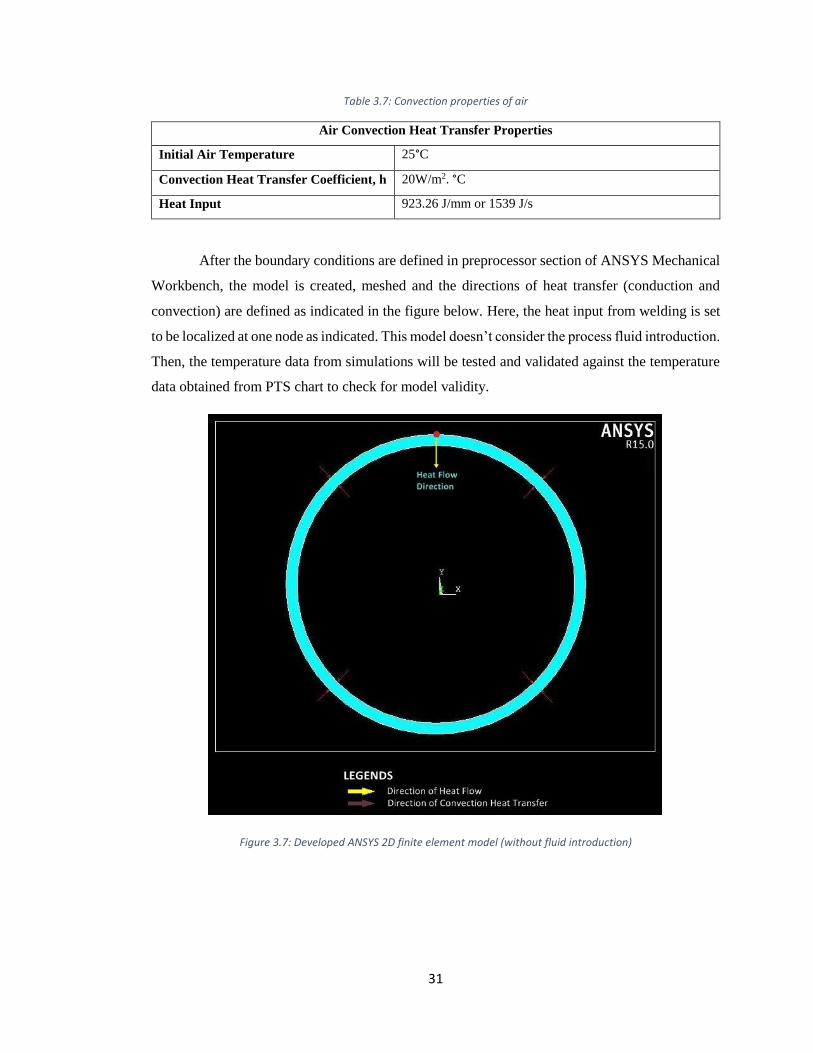
Table 3.7: Convection properties of air
Air Convection Heat Transfer Properties
Initial Air Temperature 25°C
Convection Heat Transfer Coefficient, h 20W/m2. °C
Heat Input 923.26 J/mm or 1539 J/s
After the boundary conditions are defined in preprocessor section of ANSYS Mechanical
Workbench, the model is created, meshed and the directions of heat transfer (conduction and
convection) are defined as indicated in the figure below. Here, the heat input from welding is set
to be localized at one node as indicated. This model doesn’t consider the process fluid introduction.
Then, the temperature data from simulations will be tested and validated against the temperature
data obtained from PTS chart to check for model validity.
Figure 3.7: Developed ANSYS 2D finite element model (without fluid introduction)

32
CHAPTER 4: RESULTS AND DISCUSSIONS
4.1 ANSYS Simulation Stage I: Prediction of Inner Pipe Wall Temperature
The result of the simulation are extracted and represented in the form of temperature profile as
follows.
Figure 4.1: Temperature profile showing maximum pipe wall temperature and inner pipe wall temperature
Inner pipe wall temperature, Tinner wall (located at node 7) obtained by using ANSYS
simulation is 98.318°C while the value obtained by using PTS chart is approximately 275°C.
There is a significant difference between those two numerical values. This suggest that the
modelling of heat source for this simulation model is not accurate. The heat source
visualization as localized and concentrated at one node is not practical and irrelevant to be used in
the simulation. Therefore, the solution are improved by defining more accurate heat source
distribution model. This finding related to the study that was conducted by Lima and Santos
(2016) in which they concluded that modeling of heat source must be accurate to obtain valid
results of computational models from experimental models.

33
Figure 4.2: Estimated inner pipe wall temperature from PTS chart at the same condition
Heat source modelling are corrected by defining heat source or heat flow along a path
as close as to the real welding conditions to get better results. This is because, in the real conditions,
the heat source will travel along certain path as the weld rod travels. The improved heat source
model is visualized in the figure below.
Figure 4.3: Improved heat source modelling on ANSYS 2D model

34
With the new heat source modelling definition, a number of ANSYS simulations are
conducted with variation of pipe size and pipe thickness by specifying constant welding heat input;
932.22 J/mm. The data obtained are compared with the temperature data obtained from PTS chart.
Table 4.1: Comparison of pipe wall temperature from PTS Chart with ANSYS simulation for heat input of 923.22 J/mm
Pipe Size,
in
Outer
Diameter, Do
Pipe Wall
Thickness, t
Estimated Pipe Wall
Temperature from PTS
chart,
Tinner wall (°C)
Estimated Pipe Wall
Temperature from
ANSYS,
Tinner wall (°C) in mm in mm
8 8.625 219.075 0.277 7.036 400.00 394.24
10 10.750 273.050 0.307 7.798 325.00 325.16
12 12.750 323.850 0.330 8.382 275.00 275.04
14 14.000 355.600 0.375 9.525 180.00 180.18
The new model indicated that the results are improved since that there are less variation
in terms of estimated pipe wall temperature value from ANSYS simulations with the data obtained
from PTS chart. Thus, it can be concluded that the modelling of heat source distribution for the
2D finite element of model of pipeline by specifying heat flow along a weld path are valid and
accurate. The simulations are conducted further with more variations of heat input. The results are
shown below.
Table 4.2: Inner pipe wall temperatures from ANSYS simulations for different weld heat input values
Pipe
Size,
in
Outer
Diameter, Do
Pipe Wall
Thickness, t Tinnerwall (°C)
in mm in mm HI: 800
J/mm
HI: 923.2
J/mm
HI: 1000
J/mm
HI: 1100
J/mm
HI: 1200
J/mm
8 8.625 219.075 0.277 7.036 344.64 394.24 445.15 480.40 523.66
10 10.750 273.050 0.307 7.798 280.78 325.16 360.32 399.09 445.86
12 12.750 323.850 0.330 8.382 230.92 275.04 310.01 345.56 390.10
14 14.000 355.600 0.375 9.525 136.71 180.18 207.26 242.53 277.80

35
Figure 4.4: Graph of estimated pipe wall temperature vs. pipe wall thickness
Figure 4.4 illustrates the results from performed simulations. With increased pipe wall
thickness for large pipe sizes, estimated pipe wall temperature decreases with every weld heat
input supplied to the system. The straight line curves with negative slopes indicates that estimated
pipe wall temperature are proportional to the pipe wall thickness. The simulations are proceeded
to the next stage, with introduction of process liquid.
0.00
100.00
200.00
300.00
400.00
500.00
600.00
6.000 6.500 7.000 7.500 8.000 8.500 9.000 9.500 10.000
Esti
mat
ed P
ipe
Wal
l Tem
per
atu
re,
Tflu
id (
°C)
Pipe Wall Thickness, t (mm)
Estimated Pipe Wall Temperature vs. Pipe Wall Thickness
HI: 800 J/mm HI: 923.22 J/mm HI: 1000 J/mm
HI: 1100 J/mm HI: 1200 J/mm

36
4.2 ANSYS Simulation Stage II: Prediction of Process Fluid Temperature
The result of simulations with the introduction of process fluid are represented in the form of
temperature profile and table as follows.
Figure 4.5: Temperature profile with the introduction of process fluid inside the system
Figure 4.5 shows temperature distribution profile for the developed 2D finite element
model with the introduction of process fluid filled at 50% level. The nominal pipe size is 14 in
with 0.375 in pipe thickness and heat input supplied is 800 J/mm. It is observed that the maximum
process fluid temperature (Tmaxoil = 45°C) is located on the fluid surface that is in direct contact
with pipe wall structure as shown in Figure 4.6 on the next page.

37
Figure 4.6: Locations of maximum process fluid temperature
The results for this stage of ANSYS simulations are presented in the table below with
variation of tested heat input values for specified pipe sizes. All simulations are performed for
50% filled process liquid at static condition.
Table 4.3: Estimated process fluid temperatures from ANSYS simulations for different weld heat input
Pipe
Size,
in
Outer
Diameter, Do
Pipe Wall
Thickness, t Tmaxoil (°C)
in mm in mm HI: 800
J/mm
HI: 923.2
J/mm
HI: 1000
J/mm
HI: 1100
J/mm
HI: 1200
J/mm
8 8.625 219.075 0.277 7.036 92.41 103.87 109.37 117.84 126.32
10 10.750 273.050 0.307 7.798 67.62 74.22 78.36 83.71 89.08
12 12.750 323.850 0.330 8.382 53.23 59.90 64.05 69.46 74.87
14 14.000 355.600 0.375 9.525 45.00 50.23 53.48 57.70 61.93

38
Figure 4.7: Graph of estimated process fluid temperature vs. pipe wall thickness
From the graph above, it is observed that process fluid temperature decreases with
decrease in pipe wall thickness. At supplied heat input of 1200 J/mm for 8mm pipe wall, the
process fluid temperature can rise up to around 126 °C during welding in hot-tapping at defined
conditions.
In real hot tapping application, process fluid temperature inside pipeline at same
conditions as specified in the simulation’s boundary conditions can be estimated by referring to
this graph. The input parameter that are required are the existing pipe wall thickness and supplied
weld heat input to get the process fluid temperature. Then, the estimated process fluid temperature
will be compared with the auto ignition temperature of the process fluid to determine the safe
allowable working temperature during welding. For the process fluid used in this project
simulations, the auto ignition temperature for natural gas condensate is approximately 232°C.
In practice, the estimated fluid temperature must be always kept lower below the auto
ignition temperature of the process fluid to avoid risk of explosion since that temperature can cause
the process fluid to spontaneously ignite, even without the presence of any external ignition
0.00
20.00
40.00
60.00
80.00
100.00
120.00
140.00
6.000 6.500 7.000 7.500 8.000 8.500 9.000 9.500 10.000
Esti
mat
ed P
roce
ss F
luid
Tem
per
atu
re, T
flu
id (
°C)
Pipe Wall Thickness, t (mm)
Estimated Process Fluid Temperature vs. Pipe Wall Thickness
HI: 800 J/mm HI: 923.22 J/mm HI: 1000 J/mm HI: 1100 J/mm HI: 1200 J/mm

39
sources such as flame or spark. In addition, oxygen concentration inside the pipeline also need to
be checked and considered since auto ignition temperature of a flammable liquid will decreases
as oxygen concentration increases.

40
CHAPTER 5: CONCLUSION AND RECOMMENDATION
5.1 Conclusion
The data from the simulations have provide basis on how to estimate the pipe wall temperature
and process fluid temperature during welding in hot tapping process. The first part of ANSYS
simulations conclude that the modelling and definition of heat source distribution for simulated
finite element model must be accurate in order to validate the temperature results against
temperature data obtained via PTS chart method. As for the second part of ANSYS simulations,
the estimated process fluid temperature value need to be compared to the auto ignition temperature
of tested process fluid to establish the knowledge on the safe working temperature during welding.
At any conditions, the process fluid temperature should not exceed this value to avoid spontaneous
combustion of flammable process liquid inside pipeline.
However, the results and data obtained in this project are still needed to be validated with
reliable methodologies instead of comparing with existing PTS chart as proposed in this project,
such as experimental laboratory data from acknowledged researches. The reason is that there
might be difference in test conditions and boundary conditions between the project simulations
with the methods developed by PTS team in developing the referred temperature prediction chart.
Eventhough the obtained project data might be close to the compared data from PTS chart, there
is no guarantee that the developed model is valid since the difference in terms of specified
boundary conditions for both methodologies might results in model inaccuracy or even produce
completely false simulation data.
5.2 Recommendation
In future works, the obtained project results can be improvised by providing more wide range of
data such as providing the information for extended range of supplied heat input and temperature
changes for specific process liquid level inside pipeline. In addition to temperature information,
the depth of weld penetration information can be added to the final chart to enable the weld
operator to investigate the burn-through risk during welding in real engineering application.
Furthermore, the accuracy of process fluid temperature estimation can be improved by considering
the remaining unfilled region (empty region) inside a pipeline section to be filled with process

41
liquid vapor with specific saturation level as a part of analysis in the finite element model
simulation. The presence of process liquid vapor that possesses specific value of heat transfer
coefficient will affect the heat transfer rate, thus affecting the final estimated fluid temperature as
the heat travels from outer pipe wall surface to the process fluid. This will give a close
approximation to the real situation of welding in hot tapping process.

42
REFERENCES
[1] Lima, O. L., Santos, A. B., “Mathematical Approaching and Experimental Assembly to
Evaluate the Risks of In-Service Welding in Hot Tapping,” J. of Pressure Vessel Tech., 138 (16).
pp. 1-11.
[2] Sabapathy, P. N., Wahab, M. A., and Painter, M. J., 2005, “The Onset of Pipewall Failure
During ‘In-Service’ Welding of Gas Pipelines,” J. Mater. Process. Technol., 168(3), pp. 414-422.
[3] Tahami, V. F., and Asl, M. H., 2009, “A Two-Dimensional Thermochemical Analysis of Burn-
Through and In-Service Welding of Pressurized Canals,” J. Appl. Sci., 9(4), pp. 615-626.
[4] Eager, T. W., and Tsai, N. S., 1983, “Temperature Fields Produced by Traveling Distributed
Heat Source,’’ Weld. J., 62 (12), pp. 346-355.
[5] Talbot, E., Hubert, P., Dube, M., and Yosefpour, A., 2011, “Optimization of Thermoplastic
Composites Resistance Welding Parameters Based on Transient Heat Transfer Finite Element
Modeling,” J. Thermoplastic Composite Materials.
[6] Atwa, H. A. E. A., 1993, “Study of the Effects of Defects on the Fatigue Behavior and the
Fracture Toughness for Low Carbon Steel (API 5L Grade B) Gas Transmission Pipelines”,
Engineering Fracture Mechanics, 44(6), pp. 921-935.
[7] Gomez, R., Munoz, D., Vera, R., and Escobar, J. A., 2004, “Structural Model for Stress
Evaluation of Pre-stressed Concrete Pipes of the Cutzamala System,” Pipeline Divisions Specialty
Congress.
[8] Morales, F. R., Scott, A.D., Perez, M. R., Diaz, E. M. C., and Morejon J. A. P., 2010, “Calorific
Energy Required During In-service Welding of Pipelines for Petroleum Transport,” Welding
International, 24(9), pp. 655-664.
[9] Krutz, G. W., and Sergerlind, L. J., 1978, “Finite Element Analysis of Welded Structures,”
Weld. J. Res. Suppl., 57, pp. 211-216.
[10] Bang, I. W., Son, Y. P., Oh, K. H., Kim, Y. P., and Kim, W. S., 2002, “Numerical Simulation
of Sleeve Repair Welding of In-Service Gas Pipelines,” Weld. J., 81(12), pp. 273-282.
[11] Law, M., Kirstein, O., Luzin, V., 2012, “Effect of Residual Stress on the Integrity of a Branch
Connection,” International Journal of Pressure Vessels and Piping, 96-97 (12), pp. 24-29.


