
University of Southern Queensland
Faculty of Engineering & Surveying
Investigation of Relationships between Skid Resistant
Deficient Pavement and Aggregate by GIS and Statistical
Analysis
A dissertation submitted by
Stephen John Clague
in fulfilment of the requirements of
Courses ENG4111 and 4112 Research Project
towards the degree of
Bachelor of Spatial Science Technology (Geographic Information Systems)
Submitted: October, 2005

i
Abstract The provision of a safe road network for the public is one of the areas of strategic
focus of the Queensland Department of Main Roads. One aspect that facilitates
the delivery of this objective is the maintenance of road pavement surfacings to a
standard that reduces the risk of road related accidents. Efficient and effective
management of skid resistance is one aspect that contributes to this accident risk
minimisation goal.
Skid resistance is affected by a multitude of variables that relate to factors such
as the vehicle, climate, and road surfacing to name a few. This dissertation will
focus solely on those factors that relate to the road surface. The majority of this
data is already stored in electronic form albeit in a variety of databases and
formats so a computer based approach was logical. To enable effective analysis
to occur it was necessary to integrate all data into a single environment. One way
to achieve this is through the use of a Geographical Information System (GIS).
GIS brings a powerful data integration mechanism through which analysis,
presentation and enhanced communication may occur.
The project was based on data captured in June 2004 covering 978.3 km of the
1758 km of road network that Main Roads’ Mackay District is responsible for in
Central Queensland, Australia. The project resulted in the development of an
integrated approach to the analysis of skid related issues. This was achieved
through the use of rigorous and consistent processes that support effective and
efficient skid resistance management practices in the District environment.

ii
In time trends in the rate of deterioration of different aggregates, construction
methods and seal types in different environments will be able to be established
allowing better planning of maintenance activities. From this information
guidelines will then be able to be produced for use in the Mackay District with
the knowledge gained adding to the existing body of information within Main
Roads.

iii
University of Southern Queensland
Faculty of Engineering and Surveying
ENG4111 & ENG4112 Research Project
Limitations of Use The Council of the University of Southern Queensland, its Faculty of Engineering and Surveying, and the staff of the University of Southern Queensland, do not accept any responsibility for the truth, accuracy or completeness of material contained within or associated with this dissertation. Persons using all or any part of this material do so at their own risk, and not at the risk of the Council of the University of Southern Queensland, its Faculty of Engineering and Surveying or the staff of the University of Southern Queensland. This dissertation reports an educational exercise and has no purpose or validity beyond this exercise. The sole purpose of the course pair entitled "Research Project" is to contribute to the overall education within the student’s chosen degree program. This document, the associated hardware, software, drawings, and other material set out in the associated appendices should not be used for any other purpose: if they are so used, it is entirely at the risk of the user. Prof G Baker Dean Faculty of Engineering and Surveying

iv
Certification I certify that the ideas, designs and experimental work, results, analyses and conclusions set out in this dissertation are entirely my own effort, except where otherwise indicated and acknowledged. I further certify that the work is original and has not been previously submitted for assessment in any other course or institution, except where specifically stated.
Stephen John Clague
Student Number: Q8380031
__________________________________
Signature
________________________________________
Date

v
Acknowledgements
I would like to take this opportunity to acknowledge the assistance of the
following people and thank them for their professional advice, guidance, and
continued support throughout this project:
Supervisors
• Dr Sunil Bhaskaran
University of Southern Queensland, Toowoomba
• Mr. Robert Perna
Queensland Department of Main Roads, Mackay District
Technical Support
• Mr. Ed Baran
Queensland Department of Main Roads, Pavement Testing Unit,
Brisbane
• Mr. Lex Vanderstaay
Queensland Department of Main Roads, Central Queensland
Regional Office, Rockhampton
• Mr. Jim Cran
Queensland Department of Main Roads, Central Queensland
Regional Office, Rockhampton
I would also like to thank the Mackay District and Queensland Department of
Main Roads for their continued support, to me, in the completion of this project.

vi
Table of Contents
Abstract ....................................................................................... i
Limitations Of Use ..................................................................................... iii
Certification ......................................................................................iv
Acknowledgements .......................................................................................v
Table of Contents ......................................................................................vi
List of Figures ...................................................................................... x
List of Tables .................................................................................... xii
Acronyms ................................................................................... xiii
CHAPTER 1 INTRODUCTION.............................................................................1
1.1 Introduction .......................................................................................1
1.2 Aims and Objectives ...............................................................................4
1.3 Expected Outcomes ................................................................................6
1.4 Overview of the Dissertation ..................................................................8
CHAPTER 2 LITERATURE REVIEW ...............................................................10
2.1 Introduction .....................................................................................10
2.2 Terminology .....................................................................................12
2.3 Definitions .....................................................................................14
2.4 Asset Implications.................................................................................19
2.5 Skid Resistance .....................................................................................20
2.6 Relationship between accidents and skid deficiency ...........................23
2.7 Risk Management and Legal Liability ................................................25
2.8 Surface Deterioration ...........................................................................27
2.9 Aggregate Treatments...........................................................................28

vii
2.10 Prioritisation Determination ................................................................31
2.11 Monitoring of Situation ........................................................................32
2.12 Other Factors .....................................................................................33
2.13 Geographic Information System ..........................................................35
2.14 Spatial Data Integration .......................................................................36
2.15 Conclusions .....................................................................................37
CHAPTER 3 STUDY AREA .................................................................................39
3.1 Introduction .....................................................................................39
3.2 The Mackay District .............................................................................41
3.3 The Study Area .....................................................................................45
3.4 Conclusions .....................................................................................49
CHAPTER 4 DATA SOURCES AND SOFTWARE.............................................50
4.1 Introduction .....................................................................................50
4.2 Skid Resistance Data ............................................................................51
4.3 ARMIS data .....................................................................................54
4.4 Spatial Data .....................................................................................64
4.5 Digital Video Road................................................................................66
4.6 Chartview .....................................................................................68
4.7 Databrowser and other tools ................................................................69
4.8 GIS Software .....................................................................................70
4.9 Prioritisation Software .........................................................................71
4.10 Conclusion .....................................................................................72
CHAPTER 5 METHODOLOGY & ANALYSIS ..................................................75
5.1 Introduction .....................................................................................75
5.2 Procedure .....................................................................................76

viii
5.2.1 Initial Investigations .................................................................79
5.2.2 Obtaining Information..............................................................79
5.2.3 Review and Evaluation of Information ....................................81
5.2.4 Data Creation Processes............................................................82
5.2.4.1 Wet Road Crashes Table............................................83
5.2.4.2 Inspection Priorities Table........................................86
5.2.5 Geocoding Information.............................................................90
5.2.6 Creating a MapInfo Workspace ...............................................90
5.2.7 Customise the ‘Main Roads’ Menu ..........................................91
5.2.8 Layer Control Utility ................................................................93
5.2.9 Representation of Information .................................................94
5.2.10 Data and Statistical Analysis Outcomes ..................................96
5.2.10.1 Wet Road Crash Table Analysis and Comments .......96
5.2.10.2 Inspection Priorities Table Analysis and
Comments .................................................................102
5.2.10.3 Other Accident Related Queries ..............................104
5.2.11 Investigation of Relationships between Skid Resistance
and Pavement Parameters ......................................................104
5.2.12 Field Inspection and Verification............................................108
5.2.13 Graphics Tools.........................................................................109
5.2.14 Information Outputs and Reporting ....................................110
5.2.15 Testing the System...................................................................111
5.3 Conclusions ...................................................................................111
CHAPTER 6 CONCLUSIONS & DISCUSSIONS.............................................113
6.1 Introduction ...................................................................................113

ix
6.2 Benefits ...................................................................................115
6.3 Future Directions ................................................................................116
6.4 Conclusions ...................................................................................118
REFERENCES ...................................................................................121
Appendix A Project Specifications ..............................................................124
Appendix B Skid Deficiency Spreadsheet...................................................126
Appendix C Metadata..................................................................................142
Appendix D Sample Workspace ..................................................................147
Appendix E Sample Thematic Output........................................................149
Appendix F Main Menu Customisation .....................................................151
Appendix G Geocoding................................................................................153
Appendix H Layer Tool Customisation .......................................................157
Appendix I ARMIS Database snapshots ...................................................160
Appendix J Skid Resistance Field Inspection ............................................167

x
List of Figures
Figure 2.1 Asset Lifecycle .....................................................................................14
Figure 2.2 Elements of Road Asset Management ................................................ 19
Figure 2.3 Accident Causation Factors ................................................................24
Figure 2.4 Results of High Pressure Washing ......................................................30
Figure 3.1 Queensland Department of Main Roads Regions ............................. 40
Figure 3.2 Central Queensland Region and Mackay District ..............................42
Figure 3.3 Mackay Central Business District and Environs ...............................43 Figure 3.4 State Controlled Road Network in Mackay District ..........................44
Figure 3.5 Extents of this project ..........................................................................46
Figure 4.1 Norsemeter ROAR Skid Tester ...........................................................51
Figure 4.2 Pre wetting of the test wheel ...............................................................53
Figure 4.3 ARMIS Architecture ...........................................................................55
Figure 4.4 Linear Referencing of Wet Road Crashes ..........................................56
Figure 4.5 Network Survey Vehicle ......................................................................59
Figure 4.6 Network Survey Vehicle Laser Array Configuration .........................60
Figure 4.7 Digital Video Road Viewer ..................................................................67 Figure 4.8 Chartview ............................................................................................68
Figure 5.1 Procedure for Skid Resistance Evaluation System .............................77
Figure 5.2 Additional Columns added to Seal Age dataset ..................................80
Figure 5.3 Query of the WetRoadCrashes Dataset ..............................................84
Figure 5.4 Main Roads Menu including Skid Resistance Link ...........................92
Figure 5.5 Workspace Layer Control ....................................................................93

xi
Figure 5.6 Graphics Tool Data Entry Interface ..................................................109
xii
List of Tables
Table 2.1: Investigatory Friction Levels ............................................................. 22
Table 2.2: International Friction Index Slip Speed Categories .......................... 22
Table 3.1: Local Government Authorities in Mackay District ............................43
Table 3.2: Road Sections tested for Skid Resistance, June 2004 .........................47
Table 5.1 Wet Accident Severity ..........................................................................100
Table 5.2 Driver License Demographics for Wet Accidents ..............................101
Table 5.3 Inspection Priorities of Possibly Significantly Deficient Sections.......103

xiii
Acronyms
ARMIS A Road Management Information System
INP Inner Wheel Path
OWP Outer Wheel Path
BWP Between Wheel Paths
STD Surface Texture Depth
SRD Skid Resistance Deficiency
TDist Through Distance
DVR Digital Video Road Viewer
GIS Geographical Information System
DCA Definition for Coding Accidents
LGA Local Government Authority
MapInfo MapInfo Professional
GDA Geocentric Datum of Australia
SDRN State Digital Road Network
SQL Structured Query Language
VKT Vehicle Kilometres Travelled
AADT Average Annual Daily Traffic
SPTD Sand Patch Texture Depth
PAFV Polished Aggregate Friction Value
MapView Departmental add – on MapInfo application
RIDC Road Information Data Centre
ARRB Australian Road Research Board

1
CHAPTER 1 INTRODUCTION
1.1 Introduction
The provision of a safe road network for the travelling public is one of the areas
of strategic focus of the Queensland Department of Main Roads Strategic Plan
2004 - 2009. An important aspect that facilitates the delivery of this objective is
the maintenance of a road pavement surfacing to a standard that reduces the risk
of skid related accidents. Efficient and effective management of skid resistance is
one aspect that contributes to this accident risk minimisation goal.
The Mackay District is responsible for approximately 1758 kilometres of state
controlled road network that span six local government areas over a land area of
38,410 square kilometres. This project investigates a representative selection of
these roads which total a length of 978.3 kilometres that were tested to determine
their skid resistance in June 2004.

2
The skid resistance testing was undertaken by the Departments’ Pavement
Testing Unit using a Norsemeter ROAR Skid tester. This skid tester is a variable
slip unit calibrated against units used in the Permanent International Associate of
Road Congresses (PIARC) International Trial which provides a report in terms of
International Frictional Index (IFI). This test apparatus carries out a wet test by
spraying a film of water 0.5 millimetres deep on the road in front of the test
wheel and gradually braking the wheel until lockup occurs. An average test
covers approximately 10 to 15 m of road and in network survey mode, testing at
80 to 90 km/h, an average of 1-2 tests per 100 meters are carried out.
The report produced from this testing indicated that some sections of road were
below their relevant investigatory levels and suggested that the underlying cause
of these problems needed to be determined via further investigation. It is
emphasised that there can be high variability in test results even where the same
test equipment is used (Baran, 2005). Therefore the results should be considered
solely as a highlighter of possible problem areas that require prompt inspection to
determine whether treatment is required. The report identified that
approximately 16% of the National Highway and 11% of other roads in the
District returned results below the investigatory level. In the case of the National
Highway the majority of the identified skid deficient areas were restricted to two
sections in the southern part of the District. Initial examinations of pavement
information in these areas indicated that the source of the problem appeared to be
aggregate related and recommended that this problem be further investigated.
This projects aim is to carry out the further investigation suggested on these and

3
other sections to determine the apparent primary and supplementary underlying
causes in each case.
Skid resistance deficiency is often the result of several factors in combination
rather than an individual factor. Skid resistance was described by Oliver (2002)
as a term indicating how well vehicle tyres grip the road. Factors that may
contribute to skid deficiency include seal age, surface texture, seal type,
environment (climatic), traffic volume and mix, speed environment, road
geometry, roughness, vehicle related factors and aggregate properties to name a
few.
For example we may find that an area that is identified as possibly skid deficient
also has a seal age of seven years, and marginal surface texture. Examination of
the proposed maintenance works program may indicate that this section is due to
be treated in the immediate future due to other intervention triggers such as age.
This may indicate that the section is nearing the end of its design life.
Importantly, similar sections younger than the problem section can then be
compared to establish whether the treatment interval is appropriate for the
particular situation. This allows expected performance to be compared to actual
performance which over time will allow informed management practices to be
developed. It is emphasised and acknowledged that pavements are affected by a
range of inconsistent factors during their lifetime. Therefore it is likely that only
generalist guidelines will be developed which may be of assistance as a support
for decision makers.

4
The pavement surface forms a critical component of the road network as it is
what the end user physically drives on and although lack of skid resistance does
not prevent usage of the network its presence is vitally important to the safety of
road users.
This project seeks to identify the sources of skid deficiency on the network,
suggest various options to mitigate any identified issues, and develop a uniform
process which, if followed, will allow consistent monitoring of performance,
development of standard practices, and aid in the decision making processes for
construction and maintenance resources in Mackay District.
1.2 Aims and Objectives
The aim of this project was to establish relationships between sections of
pavement with identified deficient skid resistance and their aggregate properties
through the use of a Geographic Information System (GIS). MapInfo
Professional was utilised to deliver the GIS components of the project as this
software allows the detailed analysis to be undertaken and communicated in a
user friendly way.
An additional aim of the project was to investigate the application of the
methodology developed and findings to the remainder of the road network to
determine whether predictive analysis can be applied. This will facilitate
establishment of appropriate reseal intervals that ensure that adequate skid
resistance is maintained for each pavement type. It is anticipated that before

5
confirmation and adoption of the methodology can occur a second field
collection of data will be required. This data is unlikely to be received in the
District until after the submission of this dissertation.
By delivery of this project through a GIS environment the integration of a wide
range of data from various sources into a cohesive and powerful decision support
tool was achieved. The visual aspect of the GIS environment enhances
communication and comprehension of the information required in a very simple
and efficient manner.
Specifically the objectives of the project were:
1. Formatting, collection and collation of various data and information on
pavement and event characteristics on selected road sections within the
Mackay District of the Queensland Department of Main Roads
2. Development of a spatial information system to allow integration,
analysis, presentation and assessment of a wide range of road related
parameters and in particular skid resistance.
3. Design various processes that maximise the usage of the data in the
system to assist in decision and prioritisation analysis support and works
program development.
4. Design a user friendly interface that allows a variety of Main Roads staff
with limited GIS knowledge to access the system, and
5. Design analysis tools that produce various prioritisation reports required
for district operations

6
1.3 Expected Outcomes
In June 2004 Mackay District commissioned the Departments’ Pavement Testing
Unit to carry out a Skid Resistance Survey of selected sections of roadway. This
project builds on the previous analysis and research that was completed in that
survey. The report indicated that various sections of roadway in Mackay returned
results lower than the relevant investigatory levels and were therefore possibly
skid resistance deficient. It was concluded by Baran (2004) that the likely reason
for this apparent deficiency was related to the properties of the seal aggregate
used. It is expected that this finding will be confirmed by this research.
As this was the first collection of skid resistance data in this District the best way
to examine the data in terms of effective and efficient analysis needed
determination. A methodology with defined investigatory levels had been
established by Baran (2004) but the evaluation methodology to deliver the
assessment of relative priorities had not. As skid resistance is affected by many
factors the final solution required the ability to integrate, query, analyse and
present data in an easy to understand format. These features are all available in
the GIS environment. An expected outcome of this project is the development of
a GIS system to facilitate delivery of these needs.
It is unlikely that any single contributing factor will account entirely for the skid
resistance or lack there of on a particular section of road. However, it is
important to understand what the primary underlying causation is in each case so
that should a particular consistent problem be identified it can be addressed

7
through informed management in future works. In this way asset lifespan may be
enhanced and efficient and effective asset management may take place.
Underlying causes of skid deficiency can arise due the following factors either
individually or mostly likely in combination (Oliver, 2002);
• Surface Texture is inadequate due to stone loss, flushing, and so on;
• Aggregate Polishing through normal service wearing;
• The above two factors often become a factor as the Seal Age increases;
• Construction issues relating to seal type, spray rates, and so on;
• General pavement condition - roughness, rutting, patching and so on;
• Vehicle related factors – speed, tyre construction, wear, tread and
inflation pressure;
• The particular binder used can affect the skid resistance properties of an
aggregate;
• Traffic environment including volumes, percentage of heavy vehicles,
and so on; and
• Climatic factors including regularity of rainfall and aggregate reactivity.
In general, it is expected that for this project the majority of issues identified will
be age related. This project will also examine various combinations of
relationships to establish what, if any correlations and effects are present between
factors. The spatial nature of the system should highlight any problems relating
to aggregate source through the geographical position of problem areas.

8
It is expected that the process developed will be able to be used across the
Region to evaluate this information and thereby improve asset maintenance and
management practices.
1.4 Overview of the Dissertation
Chapter 1 covers the introduction, aims and objectives, and a brief summary of
the expected outcomes of this project.
Chapter 2 encompasses the literature review with an introduction and discussion
on the importance and value of skid resistance data to the Department. Topics
covered include asset implications, discussion on significance of relationships,
prioritisation, data, and systems.
Chapter 3 provides the background to the project and a description of the
environs of Mackay around which the project is centred
Chapter 4 covers information on the project data, its’ sources, manipulation,
quality issues and the effects these have on the project. This chapter also
discusses the software used to deliver the project
Chapter 5 describes the methodology and procedures utilised in the delivery of
this project.

9
Chapter 6 surmises the conclusions that resulted from the project, as well as
commenting on the benefits of the project and possible future works.

10
CHAPTER 2 LITERATURE REVIEW
2.1 Introduction
Main Roads recognises the importance of the provision of adequate infrastructure
to support the road transport needs of Queensland. As the funding available to
develop, maintain and enhance the road network is finite in nature it is important
that decisions for works are based on appropriate priorities to ensure the
maximum benefits for Queensland are realised. The road network and its’
associated infrastructure has a total asset valuation in excess of $20 Billion (Main
Roads, Annual Report 2003 – 2004, 2004). With total annual funding of
approximately $2.3 Billion provided to carry out all works required on the
34,000 kilometres of network efficient and effective management is required to
ensure that an adequate and safe network is provided to the people of Queensland
(Main Roads, Annual Report 2003 – 2004, 2004).

11
As the majority of the network in the state is currently in a stable location the
road network could be described as relatively mature. That is, today there are
comparatively few main roads being built on new alignments compared with the
past. A large proportion of funding is therefore focussed on maintaining and
enhancing the existing asset. A key indicator used to prioritise funding is
obtained through the measurement of pavement performance against various
standards and parameters such as roughness, rutting, surface texture, and so on.
Road Safety is identified as a specific area for strategic focus in the Department
of Main Roads Strategic Plan 2004 -2009 (Main Roads, 2004). A key initiative
established to deliver the objectives of the Strategic Plan in terms of asset
management related activities is the Road System Manager (RSM) framework.
RSM provides a framework through which consistent understanding of asset
management issues and implications on departmental business may be gained
through the development of a Road System Performance Plan (RSPP). An RSSP
focuses on maximisation of whole of life performance, having regard to safety,
road user costs, community benefits, and Main Roads outlays.
Main Roads North Queensland Region based in Townsville published a strategy
that addressed a wide range of factors that relate to outcomes identified by RSM
in September, 2004. Element 29 of this strategy relates specifically to
management of skid resistance. It provides guidelines and a vision for
assessment, prioritisation, management, and performance measurement of skid
resistance. In the development of this project the outcomes and strategies
identified in the North Queensland solution were considered.

12
Pavement performance, both actual and expected is analysed using, along with
other systems, a departmentally developed package called Scenario Millennium.
This package uses a set of generic intervention levels and expected deterioration
models determined on both a state wide and local level to prioritise sections of
pavement that need treatment. The package is able to be used to analyse different
scenarios and their effects. For example, what the effect of various changes to
funding would have on the networks’ condition. It is emphasised that all the
systems involved including Scenario Millennium do not make the decisions, but
rather provide information that allows focused investigation of possible problem
areas by experienced engineers and managers. These people must take into
account a variety of factors including, expected deterioration, available funding,
political, legal and social implications to name a few in deciding the ultimate
treatment priorities.
Whilst Main Roads experiences in asset management and valuation are still in a
state of continued evolution, strong base methodologies have been enacted that
provide a clear direction for the future management of the network. This future is
likely to involve greater integration of information, data analysis, and reporting
through computer systems that enable the best outcomes to meet the
requirements of the Department and Queensland.
2.2 Terminology
Asset management has become an area of intense focus in road network
management. To enable a clearer understanding of the significance of this topic it
is necessary to examine the context of what is meant by this terminology.

13
Asset management was defined by the Departments' Roads Information Branch
(2001) as consisting of four key elements:
• Knowledge of how the system is performing including
o Condition
o Traffic
o Maintenance dollars input;
• Understanding of pavement technology and how pavements perform in
service;
• The ability to convert this information into whole of life costs and
benefits to the community at large; and
• Knowledge of how the road system can be expected to perform in the
future, under varying funding / traffic scenarios.
These elements all provide a framework within which the road, its condition,
usage, maintenance and stratagem to improve its performance can be managed.
Main Roads developed a Road Asset Maintenance Policy and Strategy (RAMPS)
in 1999 which covers the maintenance of all State-controlled road assets. This
policy defines the road asset as the pavements, bridges, surfaces, formation,
drainage structures, traffic control systems, signage, and other associated
infrastructure. Road Asset Maintenance is defined by the policy as preservation
of the serviceability, load carrying capacity, and safety of the road asset
throughout its service life and beyond. The policy describes an asset lifecycle
which is depicted in Figure 2.1.

14
Figure 2.1 Asset Lifecycle (Source: Road Asset Maintenance Policy and Strategy, 1999)
The effect that the asset lifecycle has on a particular road section relates to the
decisions made based on costs, expected deterioration rates, traffic environment
including any foreseeable changes, set trigger points for treatment, and past
experience in that environment with similar treatments.
2.3 Definitions
It is necessary to define the more tangible inputs that comprise the pavement so
that their effects on the outcomes of the project may be understood.
Pavement is defined as the portion of the road, excluding shoulders, placed above
the subgrade level for the support of, and to form a running surface for, vehicular
traffic (AUSTROADS, 1992). Subgrade level may be defined as the point of
deepest excavation of the natural landscape which forms a foundation surface on
which the pavement rests. Pavement is made up of several components of which
Asset life-cycle
PlanDesignConstruct
Operate
Maintain
Dispose
Management of ongoingperformance and condition= Road Asset Maintenance

15
the most significant for this project is the pavement surface which is composed
of aggregate and bituminous binder.
Aggregate may be defined as the predominantly uniform sized granular rock that
forms part of the pavement surface in road construction. The aggregate used on
all Main Roads projects is supplied to a standard specification which addresses
issues such as cleanliness, uniformity of size, shape, hardness, durability,
resistance to polishing and resistance to weathering. However, there are also
local factors that affect the aggregate performance in service including climatic
conditions, traffic environment, and reactivity to name a few. Several of the
properties of aggregates are important to the provision of adequate skid
resistance and are now discussed.
Surface texture of an aggregate is important on two levels, namely microtexture
and macrotexture. Microtexture refers to those aspects of the aggregate that are
less than 0.5 mm (Oliver, 2002) whilst macrotexture refers to those aspects
between 0.5 mm and 50 mm. Microtexture is key to skid performance as
aggregates with a harsh microtexture can break through a water film to give
adhesion and therefore offer better skid resistance than those with a smooth
microtexture (Oliver, 2002). Further, microtexture is responsible for provision of
adequate friction to allow the manoeuvring of a vehicle (Baran, 2005)
Macrotexture is important as it allows paths for water on the pavement to escape
from the roadway. If there is a lack of escape paths for water the skid resistance
available decreases (Oliver, 2002). The degree to which stone stands proud of the
binder surface will also have a large effect on available pathways. Kwang et al
(1992) advise that macrotexture's contribution to skid resistance is particularly

16
important in high speed environments. These two properties are the key to the
provision of adequate skid resistance.
A significant factor in the skid performance characteristics of an aggregate relate
to its resistance to polish. Polishing of aggregates occurs through the abrasive
action of traffic on the surface material. This has a tendency to smooth the
aggregate and thereby reduce its desirable microtexture properties and hence
reduce available skid resistance. An aggregate that polishes too readily will
rapidly lose its microtexture and this will result in a shorter than desired service
life.
The Standard Specifications for Aggregates specify a Polished Aggregate
Friction Value (PAFV) which should provide aggregate that has adequate
resistance to polishing. The PAFV, also known as Polished Stone Value (PSV)
provides an indication of how susceptible an aggregate is to being polished
through wearing. Baran (2005) advises that the PAFV test does not necessarily
reflect in service PAFV levels. Further that a high PAFV does not ensure a high
skid resistance. Baran (2005) concludes that PAFV is useful in ranking
aggregates but it cannot be used to predict skid performance. Oliver (2001)
advises that in Australia very high PAFV stones are not available and this is
compounded by a shortage of moderately high PAFV aggregates. Consequently
this factor may be the underlying issue in those areas which have returned results
lower than the investigatory level. The pavement surface type also has a
significant role to play in provision of skid resistance.

17
For this project the pavement surface types have been divided into two broad
categories, namely asphalt and chip seal. Asphalt seals form a complete
pavement layer and in many cases form a structural part of the pavement and are
consequently quite thick (minimum of 40 millimetres – considered structural
once >80 mm thick) whilst chip seals are generally a thin veneer like surfacing
that protects the underlying base coarse material. Generally chip seals will have a
greater surface texture depth whilst asphalt will provide a greater area of contact
at the road tyre interface. The characteristics of these two broad surfacing groups
are quite different in relation to skid resistance and therefore must be considered
separately.
As aggregate ages in a pavement it gradually becomes more polished through
wear and hence skid resistance decreases. There are a variety of factors that can
affect the in service performance of the aggregate including the binder used,
environmental factors, and the heavy loads that the pavement is subject to
(Baran, 2004). The biggest in service contributor to polishing comes from heavy
loads which can dramatically reduce the microtexture of the aggregate (Oliver,
2004). Thus an aggregate that may meet the specification in terms of PAFV may
have a lesser than expected service life if it is exposed to certain environments.
Seal related properties may affect skid resistance in several ways. Firstly, the
nature of the seal itself including aggregate size, and bituminous binder type may
have an effect on the skid resistance. Aggregate size will naturally affect the
macrotexture of the pavement surface with a larger stone generally providing
more pathways for water to escape. The contact area at the tyre / road interface
may also be significantly different between different aggregate size and

18
pavement surfaces. Bituminous binder oxidises as it ages, thereby changing its'
properties. This often results in the pavement becoming brittle which may result
in cracking and stone loss which can in turn affect skid resistance properties
through loss of contact area and macrotexture. Baran (2005) advises that skid
resistance on newly treated road sections can also be affected by the type of
binders used with polymer modified binders taking longer to wear off and
therefore allow exposure of microtexture. These factors will vary for each
combination and treatment type and are beyond the scope of this dissertation.
Seal age is defined as the period of time that has elapsed since a pavement
surface was opened to traffic (Main Roads, 2002). Seal age is important because
over time several changes can occur that affect the available skid resistance.
These include loss of stone, impaction of stone, polishing of the stone through
wear and tear, possibly flushing, increased roughness, oxidation of the
bituminous binder, and rutting. The majority of these topics have already been
discussed with roughness and rutting to be addressed later.
Flushing is defined by Transit New Zealand (2002) as a low textured road
surface due to the upward migration of binder, reducing macrotexture. Thus
surface water has fewer pathways through which to escape and resultant skid
resistance is generally lower in a flushed pavement. An indicator of skid
resistance deficiency may be the occurrence of aquaplaning and this is more
likely to occur on flushed pavements where drainage pathways are minimal.

19
Aquaplaning or hydroplaning may be defined as the partial or full loss of contact
between the tyre and the physical road surface due to surface water which
removes any braking or cornering control from the vehicle operator (Oliver,
2002). Aquaplaning is therefore the result of insufficient macrotexture.
Aquaplaning should not be confused with inundation of the road surface through
ponding or cross pavement flows when assessing skid resistance. Whilst both
involve a depth of water that results in a loss of traction the underlying cause is
slightly different. The latter is more likely related to cross pavement drainage, or
rutting issues rather than a skid deficiency issue. In both cases prompt inspection
and treatment to mitigate the issue are required.
2.4 Asset Implications
In 1997 AUSTROADS published a Strategy for Improving Road Asset
Management Practice which suggests that asset management comprises the
elements shown in Figure 2.2.
Figure 2.2 Elements of Road Asset Management
���������
������ �
���� � ���
����������� �
� ��
�������
� ��
��������� �
� ��
� �
�
��
��� ����
��������� ����
����������
�� � �
�
��
� �� ����������
�������
STR
AT
EG
Y D
EV
EL
OPM
EN
T
�����������������
���������

20
This view has been adopted as part of the departmental RAMPS initiative. The
RAMPS initiative utilises the elements described in the figure by focusing on the
effective delivery of benefits to the community. The main streams of asset
management identified by RAMPS include:
• Identification of the need for an asset based on community
requirements;
• Provision of an asset including its ongoing maintenance and
rehabilitation to suit continuing needs
• Operation of the asset; and
• Disposal of the asset when it is no longer required or appropriate
Therefore effective management of the road asset is reliant on a complete picture
of the factors impacting on the asset throughout its lifecycle. This project will
provide an additional source of input into the asset management process and
maintenance programs through a greater understanding of in service capabilities
of pavements.
2.5 Skid Resistance
Skid resistance was described by Oliver (2002) as a term indicating how well
vehicle tyres grip the road. Baran (2005) supports this view by defining skid
resistance as the contribution the road surface makes to the available friction at
the road / tyre interface. This premise will be adopted for this project.

21
Investigations into skid resistance have been carried out across the world with
much research carried out in Europe and North America. Much of this research
was carried out on concrete pavements and in climatic conditions vastly different
from those in Australia. The significant relevant factors from this research are
possible solutions with which to mitigate problem sections as well as the
development of standard skid resistance testing and in particular the derivation of
the International Friction Index (IFI). In May 2005, Baran presented findings
from the International Surface Friction Conference – Roads & Runways held in
New Zealand which suggested that IFI appeared to be the best performance
indicator for high speed roads based on a trial at the Sydney Airport. The
majority of the roads controlled by Main Roads are in high speed environments
so this choice is logical.
Baran (2004) advises that the IFI has two components, F60 and SP.
• F60 is the standardised friction measure (friction factor) at a 60
km/hr slip speed.
• Sp is the gradient of the friction versus slip speed relationship
and is an indicator of the speed dependency of the recorded
friction value. Because F60 is dimensionless Sp (expressed in
km/hr is generally referred to as the speed number. The Sp
value is only used to adjust the tolerable F60 where slip speeds
other than 60 km/hr are adopted.
Queensland Main Roads has developed Investigatory Criteria, based primarily on
the VicRoads / RTA Investigatory Criteria, for three skid resistance demand site
categories (Table 2.1) (AUSTROADS, 2005).

22
Skid Resistance Demand Category Description of Site
Investigatory Levels F60*
High
Curves with radius < 100 m. Roundabouts. Traffic light controlled intersections. Pedestrian/school crossings. Railway level crossings. Roundabout approaches.
0.35
Intermediate
Curves with radius < 250 m. Gradients > 5% and > 50 m long. Freeway and Highway on/off ramps. Intersections
0.30
Normal
Manoeuvre – free areas of undivided roads. Manoeuvre – free areas of divided roads.
0.25
*These base levels are for a 60 km/hr slip speed (appropriate for 60-80 km/hr speed zones).
Table 2.1 Investigatory Friction Levels (Source: Baran, 2004)
Baran (2005) further advises that the investigatory levels presented in Table 2.1
are only considered appropriate for 60 – 80 km/h speed zones. Because skid
resistance is dependant on slip speed, this criteria needs adjustment for other
speed zones. Adopted slip speed for speed zones are presented in Table 2.2.
Gazetted Speed (km/hr) 110 100 90 80 70 60 50 40
Adopted Slip Speed (km/hr) 80* 80* 70* 60* 60* 60 50 40
*Assumes good visibility and some speed reduction occurs before panic breaking
Table 2.2: International Friction Index Slip Speed Categories (Source: Baran, 2004)
Base F60 levels require upgrading in speed zones of 100 and 110 km/hr to reflect
the lower skid resistance available in these high speed environments (Baran,
2005). Conversely in low speed zones, Investigatory Criteria can be relaxed as
greater friction is available at low slip speeds. For speed zones other than 60 – 80
23
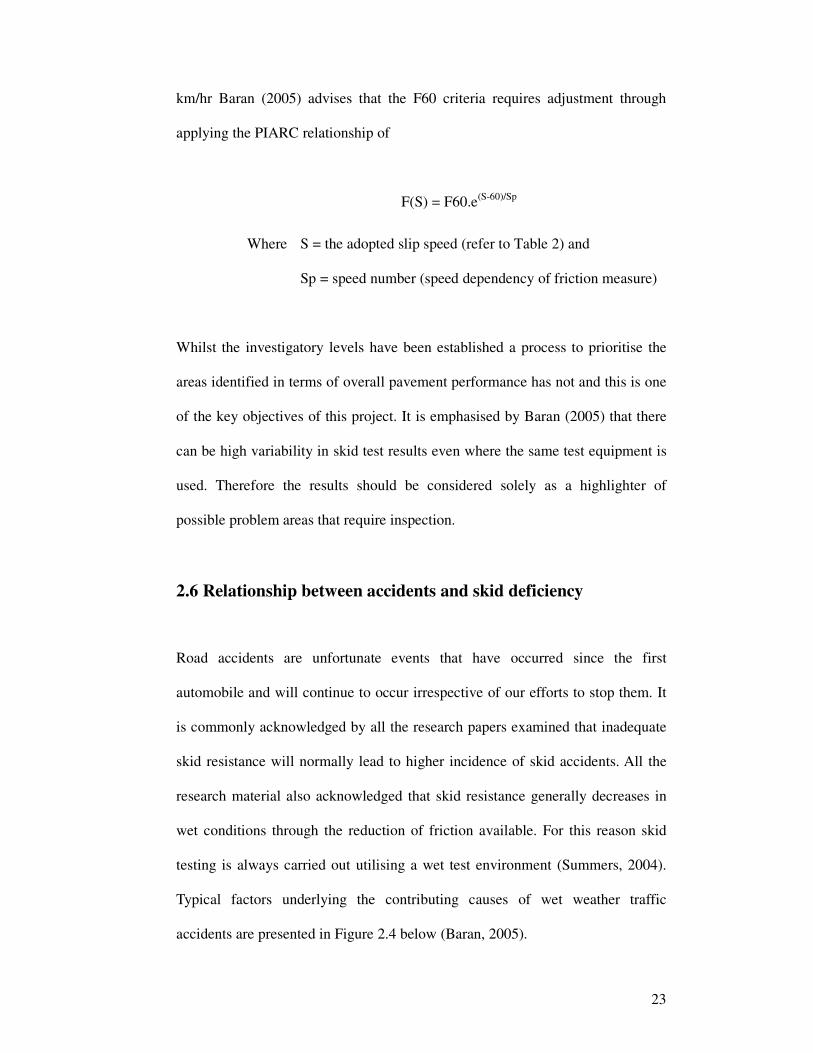
km/hr Baran (2005) advises that the F60 criteria requires adjustment through
applying the PIARC relationship of
F(S) = F60.e(S-60)/Sp
Where S = the adopted slip speed (refer to Table 2) and
Sp = speed number (speed dependency of friction measure)
Whilst the investigatory levels have been established a process to prioritise the
areas identified in terms of overall pavement performance has not and this is one
of the key objectives of this project. It is emphasised by Baran (2005) that there
can be high variability in skid test results even where the same test equipment is
used. Therefore the results should be considered solely as a highlighter of
possible problem areas that require inspection.
2.6 Relationship between accidents and skid deficiency
Road accidents are unfortunate events that have occurred since the first
automobile and will continue to occur irrespective of our efforts to stop them. It
is commonly acknowledged by all the research papers examined that inadequate
skid resistance will normally lead to higher incidence of skid accidents. All the
research material also acknowledged that skid resistance generally decreases in
wet conditions through the reduction of friction available. For this reason skid
testing is always carried out utilising a wet test environment (Summers, 2004).
Typical factors underlying the contributing causes of wet weather traffic
accidents are presented in Figure 2.4 below (Baran, 2005).

24
Road Driver Vehicle
Direct Cause 2% 71% 3%
Combined Cause 22% 1%
Don’t Know 1%
Figure 2.3: Accident Causation Factors (Source: Baran, 2005)
It is apparent from this research that although a very low percentage of accidents
are directly attributed to the road there are a significant percentage of combined
causes. These statistics support the need for regular monitoring of road surface
conditions one of which is skid resistance to ensure that a maximised level of
road safety is delivered.
Oliver (2002) advises that accidents are generally the result of a chain of events
rather than a single factor. Factors may include driver fatigue, late detection of
traffic devices, wet pavement with poor skid resistance, loss of control when
braking, driver experience, and vehicle related factors such as tyre tread to name
a few. This chain of events may be broken at many points which may avert or
reduce the severity of the accident. The speed involved in a crash may have a
significant effect on the outcomes (Oliver, 2002). Oliver (2002) concludes that
by improving the skid resistance a significant reduction in speed can be achieved
which is likely to have a substantial effect on crash outcomes. There are three

25
main approaches used to examine the relationship between skid resistance and
accidents (Oliver, 2002);
1. comparison of high accident sites with average;
2. correlate accidents and skid resistance; and
3. comparison of accidents that occur before and after treatment to improve
skid resistance.
This project predominantly uses the second approach however an investigation of
those sites on the network with high accident rates was also undertaken. Other
indicators such as police reports were reviewed to establish whether skid
resistance issues were apparent. It is emphasised that as part of normal
Departmental operations all police accident reports are reviewed and if necessary
investigated to ensure that any road related factors are identified and when
appropriate remedial action is promptly taken. This is particularly the case where
any possible road related factors are cited in the report. As there is an established
correlation between skid resistance and accidents this comprises an important
aspect of this project, of the provision of a safe road environment, and of asset
management as a whole.
2.7 Risk Management and Legal Liability
The Queensland Department of Main Roads is defined as the legal custodian of
the declared State Controlled Road Network and as such has certain obligations
and responsibilities in relation to the network, its users and the infrastructure that

26
it comprises. A key aspect of these responsibilities relates to the departments duty
of care to the public with respect to the planning, operation, and maintenance of
the network. In the past, all State Road Authorities (SRAs) in Australia were
protected by legislation from charges of negligence. However decisions in the
High Court on 31 May 2001 (Singleton Shire Council vs. Brodie and
Hawkesbury Shire Council vs. Ghantos) mean that SRAs may be subject to
common law negligence or non feasance (Oliver, 2001). It is acknowledged that
the road does not have to be perfect but demonstration that reasonable measures
have been taken to maintain a standard is required. Therefore failure to discharge
this duty of care in an appropriate manner may result in the department being
exposed to litigation if it or its agents are seen as negligent in their actions in a
particular instance and set of circumstances.
As a methodology to minimise and manage risk the Department has always
carried out regular field inspections and evaluations of how the asset is
performing, sought to proactively identify potential problem areas, and
expediently address any issues found. An area of strategic focus for the
Department is the provision of a safe road network which is addressed through
the Road Safety component of the Road System Manager framework.
Risk management was defined by DETIR (2000) as the identification,
assessment, development and implementation of control measures and review of
potential hazards that may arise during the execution of a task. The key factors in
managing risks associated with skid deficiency are multi-faceted and as such
vary from case to case. However, by the use of investigatory levels that relate to

27
the specific environment it is possible to identify potential problem areas. This
information when combined with field inspection, engineering input, other
pavement information and parameters allows the relative priorities of each road
section to be effectively evaluated.
A key aim of this project will be the development of a methodology to assess
relative skid deficiency priorities. This approach should facilitate the realisation
of a strategy that encompasses a wide range of factors and enables maximum
benefits and outcomes for the general public. Decision makers will have a clear
picture of the impacts that skid resistance has on the network and the underlying
factors that need to be managed to ensure that the risks in these areas are either
mitigated or removed in an appropriate and timely manner. This results in the
added benefit of reducing the risk of litigation and follows the ideals of the asset
management philosophy.
2.8 Surface Deterioration
Pavement surfaces naturally deteriorate as they age due to a wide range of factors
in their service environment. This usually results in a loss of both microtexture
through the polishing effect of traffic and macrotexture through stone loss or
impaction, pavement flushing and wear (Oliver, 2002). These factors are affected
by the characteristics of the pavement surface, climatic, and traffic environment.
It is critical for effective asset management that strategies are in place that allow
prioritisation of areas so that desired standards may be maintained. This is
achieved through the use of a Pavement Management System (PMS) which

28
identifies the nature and timing of pavement treatments (Main Roads, 2001).
Main Roads developed Scenario Millennium which is such a PMS. Scenario
Millennium utilises a set of predetermined trigger points and expected
deterioration rates related to various attributes of the pavement to devise a list of
priorities. The information extracted from this system is utilised to aid in the
decision making processes for the maintenance works programs. This system
does not currently consider skid resistance in the development of priorities. Skid
resistance is a pavement attribute that has a valid role in the prioritisation of road
maintenance works programs (Oliver, 2002).
2.9 Aggregate Treatments
If the goal of effective and efficient asset management is to be achieved, it is
vital that the most appropriate treatments for each situation are utilised. A key
aspect of this is the monitoring and evaluation of in service pavement
performance against expected standards. The aggregate used has a significant
role in the performance of a particular treatment and is assessed against a
detailed specification. In most cases there is a variety of differing treatment
options available to the Engineer, each of which will provide different qualities
in the finished product for varying costs. Different treatments may also involve
different aggregate mixes and so significant differences can occur based on the
treatment used. If a treatment is ineffective there is recognition that the practices
in place require review to ensure that performance is maintained and inefficient
practices cease. It is also vital that a complete picture of all desired performance

29
parameters of the pavement is gained to facilitate a solid decision making
process.
Baran (2005) advises that there are a variety of different treatments available that
generally focus on improving the micro and macrotexture of the pavement
thereby increasing the skid resistance available. These include;
1. High pressure washing of the existing pavement to improve the available
pathways through which water can exit the pavement. Figure 2.4 shows
an example of the results of this treatment type. Note the greatly
improved macrotexture on the treated (right side) of the photo. This
treatment is quite expensive, but is also effective in extending the useful
life of the surface. There are some additional negative effects related to
the reduction of binder in the pavement which may allow moisture
penetration into the underlying pavement;
2. Calcinated Bauxite is added to the regular aggregate mix. This material is
very durable and has a high microtecture and macrotexture quality. It is
however expensive;
3. Grooving of the pavement using a pavement profiler to create additional
drainage pathways. This treatment is primarily utilised on concrete and
asphalt surfaces to improve macrotexture; and
4. Carrying out a secondary seal with smaller rock of the same material
which improves skid resistance through additional tyre / pavement
contact area whilst maintaining similar macrotexture properties.

30
Figure 2.4 Results of High Pressure Washing (Source: Main Roads, Emerald)
It should be noted that mitigations other than reseals are also used to manage skid
resistance. Measures such as warning signage, speed restrictions, changes to
cross pavement drainage, and reducing manoeuvring demands all play important
roles in the management of skid resistance.
The Department is constantly examining ways to improve pavement performance
through research by the Pavement Testing Unit and field testing and trials of
various treatment options by Districts. The findings of research are regularly
disseminated throughout the Department so that optimal practices are
maintained. Aggregate treatments and selection of the right aggregate for the
particular environment are critical to the in service pavement and skid resistance
performance.

31
2.10 Prioritisation Determination
A risk based intervention strategy is utilised by Main Roads throughout the
majority of its management systems. In the case of skid resistance, departmental
investigatory levels have been established for differing environments. However,
pavement maintenance prioritisation involves a wide variety of factors some of
which are based on subjective assessments. One of the expected outcomes of this
project is to establish any trends between various pavement factors. For example,
a trend where the skid deficient sections are all over a certain age on a certain
section of road may indicate that the expected useful pavement life has been
exceeded, especially if other indicators are also poor. In this way the treatment
regime for the particular environment may be adjusted.
Prioritisation of pavement sections is therefore a multi facetted process with
those sections that have multiple issues identified being likely to be targeted for
treatment prior to those that have one defect. For example, if all skid deficient
pavement on a particular road section is over a certain age, has high roughness
and deep rutting it is likely to receive a higher priority than a section which has
just one of these factors.
When the skid data is received from the field it is evaluated to establish whether
there are any sections requiring immediate investigation (Baran, 2004). This
initial investigation involves checking the sections for any apparent skid related
accident history, visual inspection, checking whether the section is programmed
to be treated, and comparison against other pavement parameters (Main Roads,

32
2004). As previously discussed all road accidents and in particular those where
the road condition has been cited as a possible contributing factor in the police
report receive prompt investigation with any remedial works required carried out
as soon is practical. The skid data is also examined to ensure that an appropriate
IFI has been used for each section as the data is not adjusted for sections where
the practical speed is lower than the gazetted speed. Therefore where a mountain
range section exists for example that is able to be negotiated at a maximum speed
of 60 km/h yet the gazetted speed of the road section is 100 km/h the IFI used
may be incorrect resulting in a deficient section being identified where there is
none. This is because the field capture does not take into account advisory speed
signs that exist within the gazetted speed zones. Appropriate prioritisation of
problem areas of the road network is a key factor in the delivery of effective and
efficient asset management.
2.11 Monitoring of Situation
This project is based on the first skid resistance data captured in Mackay District
and as such this data will form a base for comparison with future capture
programs. It is anticipated that over time trends will be able to be determined that
will allow useful life guidelines to be determined for each aggregate and
construction methodology combination. How these expected useful life
guidelines will compare to other existing treatment triggers is unknown.
Oliver (2002) suggests that for surfaces greater than five years old it is important
to monitor whether the crash rate is high or increasing which may indicate that

33
skid resistance is becoming an issue. There are a range of factors that affect the
rate of deterioration of the road surface such as traffic environment, climate,
aggregate properties and construction method to name a few and so it is
important to proactively monitor the condition state of the road asset.
2.12 Other Factors
Oliver (2002 identified a variety of other factors that may significantly affect the
roads skid resistance properties. These include climate, traffic environment, tyres
and construction methods each of which will now be briefly discussed.
Climate has several potential influences. Oliver (2002) advises that skid
resistance can improve when regular rainfall occurs as the pathways through the
pavement and microtexture of the aggregate are cleaned. Conversely during long
dry periods skid resistance may reduce as the surface becomes clogged with
detritus material and the stone polished. Oliver (2002) also advises that as
temperature increases skid resistance tends to decrease. Baran (2005) advises that
although limited data is available for Queensland conditions it is apparent that
the effects of temperature appear minimal. This finding was based on an ARRB
study (Oliver et al, 2002) that concluded that in all states except Queensland,
there is substantial seasonal variation in skid resistance. Baran (2005) concluded
that no correction for temperature need be applied when considering skid
resistance in Queensland.

34
Reactive aggregates and environments may also affect the performance of a
pavement through chemical reactions that affect the durability of the aggregate
and thus its susceptibility to polishing and failure. These agents may also affect
the binder through chemical reactions. These issues are normally considered and
where required addressed during seal and pavement design.
The volume and type of traffic can have a significant effect on skid resistance.
Main Roads attempts to compensate for the traffic environment related issues
through the design of appropriate pavements. Oliver (2002) commented that
sudden changes in traffic volume can also change the skid resistance properties
of a section of road. Oliver (2002) advises that heavy vehicles are a major cause
in the loss of microtexture in pavement surfaces through polishing. Skid
resistance properties also vary considerably between pavement types and hence
construction methods adopted will affect the useful life of the road section.
Appropriate pavement design should minimise these issues.
Vehicle tyres have a crucial role to play in skid resistance as they are the point of
contact between the vehicle and pavement surface. Factors such as the
construction of the tyre, tyre wear, rubber in tread and inflation pressure all affect
skid resistance (Oliver, 2002). As these factors are variable and no data is
available on the test sections on these parameters they are acknowledged but will
not be considered further in this dissertation.

35
2.13 Geographic Information System
Geographic Information Systems (GIS) are a powerful set of tools that facilitate
the capture, input, data management (storage and retrieval), manipulation and
analysis, and outputting of geographical data (Clarke, 1997). Geographical data
may be described as data about an objects’ spatial position relative to a known
reference system, its relationship to other objects around it, and its associated
physical attributes. GIS differs from other information systems such as
spreadsheets through its ability to deal appropriately with spatial information
which these other systems do not adequately cater for. GIS allows greater
visualisation and enhanced communication than the tabular displays of other
systems through its ability to create easy to understand map and graphical
outputs. The ability to share maps through the digital environment whilst
maintaining the ability to produce hard copy outputs is another key advantage of
these systems.
The integration of a wide range of data into a single cohesive framework that
allows the viewing of relationships between various attributes is a powerful
feature of GIS which can facilitate informed decision making based on a broad
view. The data used can be accessed in both tabular (textural or numeric) or
geographical form (map objects) which allows collation of a wide range of
information. Documents may also be ‘hot linked’ as attachments to map objects
which allows more information to be accessed at the click of a button from
within the package. GIS also offers an ability to query and interrogate spatial and
statistical data based on user defined scenarios which may aid in decision making

36
processes. The power of GIS as a data integrator, analysis and presentation tool
make it an ideal choice for this project.
The GIS package utilised for this project is MapInfo Professional Version 7.5
which is a desktop level mapping application. This package provides the level of
functionality required for this project in a user friendly manner and is currently
widely available across Main Roads through an unlimited usage corporate
licensing agreement. Over a period of time Main Roads has developed a series of
tools to assist in the use of MapInfo for departmental needs. These tools are
collectively known as the “Nerang Applications” in recognition of the District
where the majority were developed. Main Roads asset information is currently
based on a linear reference system and these tools utilise dynamic segmentation
to produce the graphical representations of this data along the relevant road
section.
In a linear reference system characteristics are described and located based on the
distance along a linear feature, in this case a road. This approach to the mapping
of data provides a viable conduit by which road asset data may be associated
with other geographical data to enable effective and efficient decision making.
2.14 Spatial Data Integration
Spatial data integration is one of the key advantages of the GIS approach to this
project. Not only in terms of the combinatorial ability to display the data but also
because of the wide range of reporting formats available to enhance and
communicate information on the particular focus of the display. A key benefit of

37
integration is that the end user can visualise and gain an insight and clear
understanding of complex relationships between the different datasets at a level
that is not as available in traditional non-spatial databases. The strength of the
GIS environment is the ability to bring data together into a single environment.
This is particularly important for aiding in understanding multi facetted problems
such as skid resistance.
2.15 Conclusions
The Department recognises that the delivery of a high level of road safety and
services to the people of Queensland is achievable through the efficient and
effective maintenance of the road asset. Asset management’s influence on the
operations of the Department is ever increasing and is the key to the delivery of
this objective.
Main Roads and indeed all state road authorities have legal and moral obligations
to proactively identify and manage all risks that may occur through the operation
of their networks. These obligations include ensuring that strategies are
implemented that outline identification, management, investigation, and
remediation of defects in an appropriate manner. Main Roads has provided
guidelines to address the gamut of road asset management issues through its
Strategic Plan and Road System Manager Frameworks.
The testing and evaluation of skid resistance data is one aspect which can
contribute to the delivery of a safe road network. Skid resistance of road
pavements is a complex issue due to the wide range of factors that influence this

38
attribute. Investigatory levels have been adopted with respect to the acceptable
minimum skid resistance recommended for each road environment. It is critical
to note that a test of skid resistance that indicates a section does not meet the
relevant investigatory level only indicates that immediate investigation is
warranted.
GIS allows effective management of spatial data and is an ideal platform for the
examination of road asset information. Data integration facilitated by the GIS
environment allows the development of a more complete appreciation of the state
of the asset by the end user through bringing together many factors into a single
environment. The visual impact of a map which shows how different factors
interrelate enhances communication and understanding of the relationships being
examined in ways not easily achieved through other means. The GIS
environment provides a powerful tool for end users in the delivery of efficient
and effective asset management.

39
CHAPTER 3 STUDY AREA
3.1 Introduction
The Mackay District located in the Central Queensland Region of the
Department of Main Roads is one of fourteen Districts that combined form four
Regions that cover the entire state of Queensland (Figure 3.1). The other regions
are Northern Queensland, Southern Queensland and South East Queensland.
Examination of the State Digital Road Network indicates that there is currently
approximately 255,000 kilometres of road casements in Queensland. Of this
figure approximately 175,000 kilometres contain constructed public roads. Main
Roads owns, manages, and operates the declared State Controlled Road Network
which comprises over 34,000 kilometres of these roads with the remainder being
under the control of Local Government Authorities. The network administered by
the department comprises the major highways that link communities across the
state, state strategic, arterial and sub arterial road networks.

40
Figure 3.1 Queensland Department of Main Roads Regions
Several key initiatives identified in the Departments Strategic Plan (2004 – 2009)
are delivered by the Department for the Queensland road system including:
• safer roads to support safer communities;
• fair access and amenity to support liveable communities;
• building Queensland's regions;
• efficient and effective transport to support industry competitiveness and
growth; and
• environmental management to support environmental conservation.
�
South East Queensland Region
Southern Queensalnd Region
North Queensland Region
Central Queensland Region
TOOWOOMBA
ROMAGYMPIE
BRISBANE
WARWICK
BARCALDINEEMERALD ROCKHAMPTON
CAIRNS
CLONCURRY
TOWNSVILLE
MACKAY
BUNDABERG

41
3.2 The Mackay District
The Region stretches from North of Proserpine in the North to South of Miriam
Vale in the South and West to the Queensland – Northern territory border
covering an area of 576,488 square kilometres and a population of 300,000
(Main Roads - Roads Implementation Program 2004 – 05 to 2008 - 09, 2004) . In
this area there are a diverse range of industries, environments and communities
ranging from sparsely populated arid farming lands in the west to densely
populated coastal cities with substantial rainfall. Major industries in the Region
include mining, crop farming, sheep and cattle grazing, and tourism. The Central
Queensland Region is directly responsible for 9916 kilometres of State
Controlled Road Network which includes 1400 kilometres of National
Highways. Mackay District is on of four districts in the Central Queensland
Region with the others being Central West, Central and Central Highlands
Districts (Figure 3.2). Mackay is located on the coast approximately 1,000
kilometres north of Brisbane
The Mackay District is centred on the City of Mackay which is a modern,
progressive city of approximately 78,000 people, located on the Pioneer River in
Central Queensland. Mackay District covers a land area of 38,410 square
kilometres and encompasses six Local Government Authorities from Whitsunday
Shire in the North to Broadsound Shire in the South to Nebo Shire in the West.

42
Figure 3.2 – Central Queensland Region and Mackay District
The city is relatively spread out with the core urban area covering
approximately137 square kilometres. Mackay is a commercial centre servicing
the Mackay and Whitsunday Region, Bowen Basin Coal fields and hinterland.
The city is surrounded by a variety of industries including intensive agriculture
based on the sugar and beef cattle industries, mining industry, port facilities for
the sugar and mining industries, and tourism related activities. The urban areas
are surrounded by highly productive agricultural lands (See Figure 3.3).
The region is the one of the largest sugar cane growing areas in Australia, second
only to the Burdekin. Mackay is home to two of Australia’s four Sugar
Refineries and the largest bulk sugar terminal in the world with 8 million tonnes
exported though the port in optimum growing years.
�
Central Queensland RegionCentral Highlands District
Central Western District
Mackay District
Central District
EMERALDBARCALDINE
ROMA
TOOWOOMBA BRISBANE
GYMPIE
BUNDABERG
ROCKHAMPTON
MACKAY
TOWNSVILLE
CLONCURRY

43
Figure 3.3: Mackay Central Business District and Environs (Source: Courtesy of Wricor Photography)
The nearby Dalrymple Bay and Hay Point Coal loading terminals situated at the
Port of Hay Point form one of the largest coal loading terminals in the world.
Currently the terminals deliver a combined total of 80 million tonnes of coal to 8
countries around the world each year. The Dalrymple Bay facility is currently
being expanded to cater for an additional capacity.
There are six Local Government Authorities encompassed in Mackay District
(Table 3.1).
Mackay City Council Whitsunday Shire Council Mirani Shire Council
Nebo Shire Council Sarina Shire Council Broadsound Shire Council
Table 3.1: Local Government Authorities in Mackay District

44
Mackay District is responsible for approximately 1758 kilometres of declared
State Control Road Network of which 1532.6 kilometres are sealed (Figure 3.4).
Figure 3.4: State Controlled Road Network in Mackay District
Whitsunday Shire
Mirani Shire
Nebo Shire
Broadsound Shire
Sarina Shire
Mackay City
Central District
EMERALD
MACKAYHABANA
MIRANI
EUNGELLA
AIRLIE
SARINA
CARMILA
CLAIRVIEW
DYSART
GLENDEN
ILBILBIE
MIDDLEMOUNT
NEBO
PROSERPINE
ST LAWRENCE

45
On these sealed roads there are 16 different surface seal treatment types that may
be loosely grouped as either asphalt or chip seal treatments. The District
currently has a total of approximately 225.5 kilometres of unsealed roads, 97.1
kilometres of asphalt with the balance being chip seal. The District is responsible
for a total of 339 kilometres of National Highway.
3.3 The Study Area
The study area for this project was adopted to match the extents of the skid
resistance testing project carried out in the District in June 2004 (Appendix B).
The areas chosen for skid resistance testing were selected based on a series of
predetermined factors and requirements which related to perceived risk exposure.
Generally these areas were in high rainfall (>800 mm per year), high traffic and
coastal areas which are considered areas of highest risk. The sections chosen total
978.3 kilometres of road network and extend to areas in each of the six local
government areas. The test locales are highlighted in Figure 3.5 as those sections
of network with a solid black linestyle.
Of the roads tested 16% of the National Highway and 11% of other roads
recorded skid resistance results below the investigatory levels. The investigation
of these sections is the focus of this investigation. The investigation of these
sections is the focus of this investigation.

46
Figure 3.5: Extents of this project
Adjacent land use varies from urban housing through to rural farming, with
traffic volumes varying from an AADT of 30 to greater than 32,000 vehicles per
day. The major urban centres in the study area include Mackay, Proserpine,
Sarina, Nebo, Airlie Beach, Marian and Mirani. Details of roads sections and
respective lengths tested are shown in Table 3.2. It should be noted that in some
cases only selected sections of the road are tested.
Whitsunday Shire
Mirani Shire
Nebo Shire
Broadsound Shire
Sarina Shire
Mackay City
MACKAYHABANA
MIRANI
EUNGELLA
AIRLIE
SARINA
CARMILA
CLAIRVIEW
DYSART
GLENDEN
ILBILBIE
MIDDLEMOUNT
NEBO
PROSERPINE
ST LAWRENCE
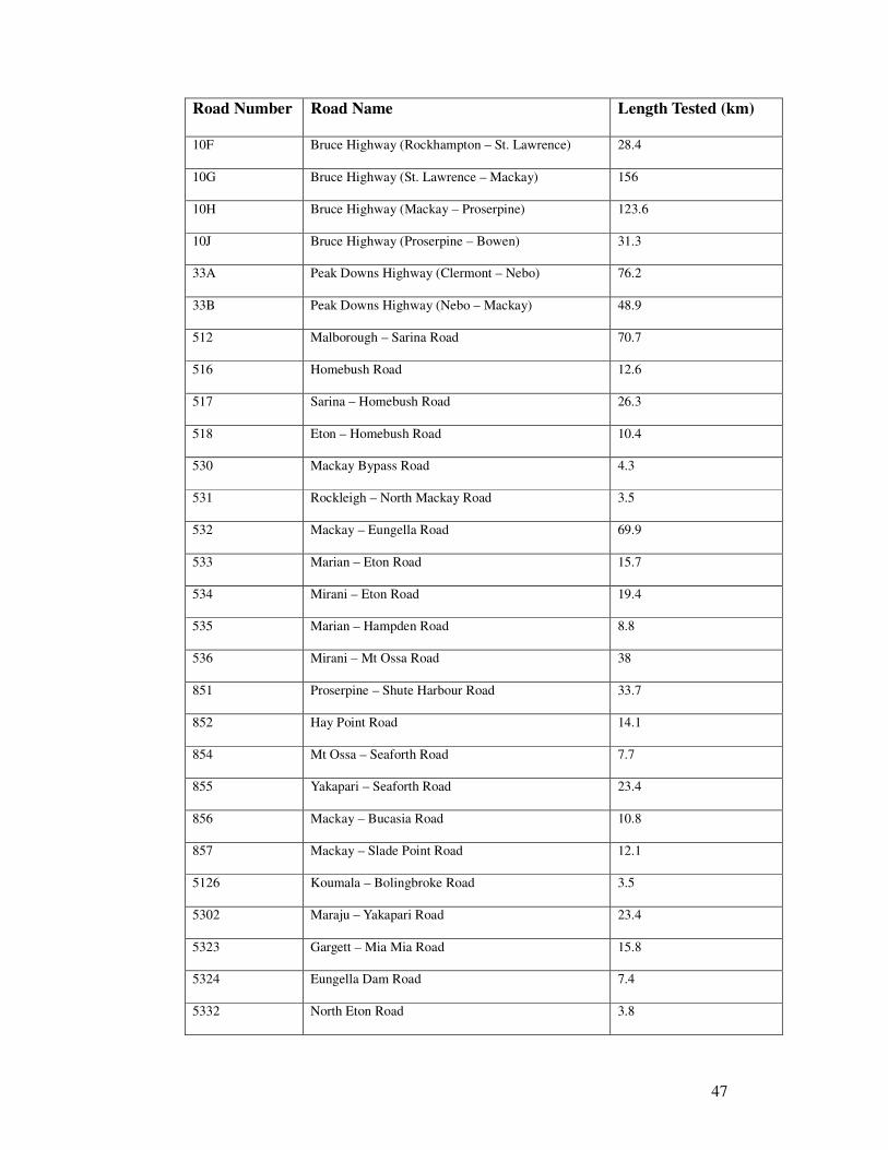
47
Road Number Road Name Length Tested (km)
10F Bruce Highway (Rockhampton – St. Lawrence) 28.4
10G Bruce Highway (St. Lawrence – Mackay) 156
10H Bruce Highway (Mackay – Proserpine) 123.6
10J Bruce Highway (Proserpine – Bowen) 31.3
33A Peak Downs Highway (Clermont – Nebo) 76.2
33B Peak Downs Highway (Nebo – Mackay) 48.9
512 Malborough – Sarina Road 70.7
516 Homebush Road 12.6
517 Sarina – Homebush Road 26.3
518 Eton – Homebush Road 10.4
530 Mackay Bypass Road 4.3
531 Rockleigh – North Mackay Road 3.5
532 Mackay – Eungella Road 69.9
533 Marian – Eton Road 15.7
534 Mirani – Eton Road 19.4
535 Marian – Hampden Road 8.8
536 Mirani – Mt Ossa Road 38
851 Proserpine – Shute Harbour Road 33.7
852 Hay Point Road 14.1
854 Mt Ossa – Seaforth Road 7.7
855 Yakapari – Seaforth Road 23.4
856 Mackay – Bucasia Road 10.8
857 Mackay – Slade Point Road 12.1
5126 Koumala – Bolingbroke Road 3.5
5302 Maraju – Yakapari Road 23.4
5323 Gargett – Mia Mia Road 15.8
5324 Eungella Dam Road 7.4
5332 North Eton Road 3.8

48
5342 Mia Mia Connection Road 5.1
5382 Crystal Brook Road 24.6
8501 Gregory – Cannon Valley Road 13.4
8506 Mackay – Habana Road 10
8509 Sarina – Coast Road 12.9
8554 Yakapari – Habana Road 8
8565 Eimeo Road 4.6
Table 3.2 – Road Sections tested for Skid Resistance, June 2004
Although in the past consistent maintenance programs for treatment based on
expected pavement life were carried out, this was based on local experience and
visual inspection. In more recent times corporately developed systems with
specific rules and triggers have been used in combination with local knowledge
to determine program priorities. This approach is aimed at allowing comparisons
of relative priorities across District and Regional boundaries and additionally as a
way to measure the effectiveness of different treatment methods utilised. This
approach has resulted in an increase in the length of time between treatments in
many cases. The effect of this approach on the pavement performance was only
known subjectively through field inspection.
Skid resistance had not been tested in this Region previously and as such the
results provide another source of information for consideration by decision
makers. On initial inspection of the results it was immediately apparent that some
sections recorded results lower than the suggested investigatory levels which
made it imperative to determine the underlying causation in each case.

49
3.4 Conclusions
Main Roads owns, manages, and operates the declared State Controlled Road
Network which comprises over 34,000 kilometres of roadways.
The Mackay District located in the Central Queensland Region of the
Department of Main Roads is one of fourteen Districts that combined form four
Regions that cover the entire state of Queensland. The District encompasses six
local government authorities with 1758 kilometres of declared State Control
Road Network under its’ control.
The project area contains areas within all six local government authorities and
comprises a total of 978.3 kilometres of declared State Controlled Road Network.
Of the roads tested 16% of the National Highway and 11% of other roads were
found to have record a result lower than the investigatory level for their
particular environment. These investigatory levels are utilised to highlight
specific areas requiring immediate inspection, however due to the variability of
results and multi factor nature of skid resistance it is emphasised that this may
not necessarily result in a requirement to treat a road section.

50
CHAPTER 4 DATA SOURCES AND SOFTWARE
4.1 Introduction
The finance and resource constrained environment that the Department exists in
means that problem areas must be prioritised based on the seriousness of their
effect on the wider network. In practice this means that an incremental program
of works is carried out over a period of years with the highest priorities addressed
first. To achieve efficient and effective prioritisation of works a considerable
amount of data must be collected, collated, analysed, problems areas identified,
prioritised, works programmed and then actioned.
It is important to note that the data contained in many of the systems is imperfect,
in some cases of low quality or incomplete and for this reason a high degree of
subjective assessment, inspection and local knowledge of the network is required
for the development of appropriate priorities. In the majority of cases the data is
captured in one traffic lane only and has been assumed to be similar for adjacent

51
untested lanes. This assumption may not be universally valid and hence further
detailed analysis is required of sections that involve such lanes.
Skid resistance is just one of numerous parameters and data sources considered
in development of the works program. Apart from road surface conditions of
which skid resistance is just one, other factors such as new developments or
growth factors in an area, structure (bridges and culverts) conditions, traffic
patterns, political imperatives and other parameters all impact on the overall
prioritisation of works.
4.2 Skid Resistance Data
Skid resistance data was captured using a Norsemeter ROAR Skid testing device
(Figure 4.1).
Figure 4.1: Norsemeter ROAR Skid Tester (Source: Courtesy E. Baran)

52
This device produces a report based on the PIARC International Friction Index.
The data was captured in the outer wheel path which is often an area where
pavement problems such as rutting first become apparent (Baran, 2004). This test
apparatus carries out a wet test by spraying a film of water 0.5 millimetres deep
on the road in front of the test wheel and gradually braking the wheel until
lockup occurs. An average test covers approximately 10 to 15 m of road and in
network survey mode, testing at 80 to 90 km/h, an average of 1-2 tests per 100
meters are carried out.
As with all field captured data there are some possible sources of error which can
affect the data. One notable problem with skid data is that if the gazetted speed
value is higher than a road user would normally be able to attain then the results
may be erroneous. Examples of such events may be range sections where the
gazetted speed may be 100 km/h but the fastest it is possible to drive is say 60
km/h. Often these sections have advisory speed limits however these are not able
to be taken into account during the capture process. This means that the “f”
(friction) value of the IFI used may be incorrect for the particular section. There
may also be tracking errors where the operator has drifted slightly from the
desired test position on the road, or places where the water sprayed in front of the
test wheel had dispersed prior to the test wheel contacting the area. Sections of
high roughness may also have an impact on skid resistance test outcomes. It is
important to note that the data presented may be the result of several tests that are
averaged over a section. The repeatability of the testing in terms of consistency is
another area of concern as high variability in results over the same sections has
been exhibited in testing. Generally 20% of road sections receive additional

53
testing. Therefore, it is emphasised that a test result lower than the investigatory
level only highlights that there is a need to investigate what may be a possible
problem.
Figure 4.2 shows the mechanism for pre wetting the pavement in advance of the
test wheel.
Figure 4.2 Pre wetting of the test wheel (Source: Courtesy E. Baran)
The areas chosen for skid resistance testing were selected based on a series of
predetermined factors and requirements. Generally the roads tested were in high
rainfall / high traffic coastal areas where a likely higher risk profile was
expected. The sections in Mackay District chosen comprise a total of 978.3
kilometres of the network and involve some areas in each of the six local
government areas. The testing report identified 16% of National Highway and

54
11% of other roads in the District where the skid resistance was below the
investigatory levels and required further investigation. This premise forms a
primary aim of this project.
4.3 ARMIS data
A key repository of road related data held by the Department is ARMIS which
stands for ‘A Road Management Information System’. This system is comprised
of a variety of Oracle based databases which were developed by the Department
and initially introduced in 1992. The system replaced the chart based system
known as CHIMPS. The system has undergone many changes since its
implementation including the addition of several new databases and a move
towards a more user friendly graphical user interface (GUI).
As with all database systems ARMIS has the capability for collection, collation,
storage, editing, retrieval, auditing, recording of metadata and reporting of road
related data that is useful in the decision making processes of Main Roads.
Although the data in ARMIS is being continually improved there are various
issues that affect the data accuracy and quality that must be understood. An
outline of the system components is shown in Figure 4.3.

55
Figure 4.3: ARMIS Architecture (Source: Roads Information Branch – Main Roads)
The ARMIS databases include detailed information on the condition, location,
and details of all road assets from signage through to major structures that
together make up the road infrastructure of the network. This data is all related
using a linear reference system that relates the physical location of each asset
relative to the defined start of the road which is described using the term Tdist.
Tdist stands for through distance. For example, for each of the wet road crashes
shown in Figure 4.4 below each has through distance (Tdist) that relates to the
start of the road. The data shown in the example has been mapped against a
constructed road centreline dataset based on the centre of road casement
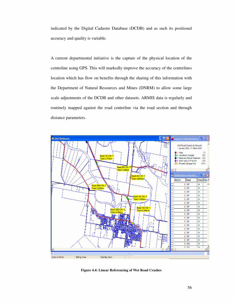
56
indicated by the Digital Cadastre Database (DCDB) and as such its positional
accuracy and quality is variable.
A current departmental initiative is the capture of the physical location of the
centreline using GPS. This will markedly improve the accuracy of the centrelines
location which has flow on benefits through the sharing of this information with
the Department of Natural Resources and Mines (DNRM) to allow some large
scale adjustments of the DCDB and other datasets. ARMIS data is regularly and
routinely mapped against the road centreline via the road section and through
distance parameters.
Figure 4.4: Linear Referencing of Wet Road Crashes

57
In this project data from a variety of ARMIS subsystems was utilised and each is
now discussed. The vast majority of construction or maintenance operations
carried out on any part of the road network will provide input to several ARMIS
subsystems. In the case of construction related projects a wide variety of
information is entered including pavement type and layer thickness, construction
methods and completion date, costs, lane, seal and formation widths to name a
few. From this information the user is able to view a wide variety of data which
may be either derived or real. Two such project related parameters are Seal Age
and Seal Type.
Seal age is defined as the time between the project completion date and the
current date. For this project the 30 June 2004 was used as the date for
determination of seal age which approximated the date of skid data collection.
This is a significant variable for this project because there are a variety of factors
such as stone polishing, stone loss or impaction, roughness, rutting, seal ductility,
and porosity that change as the pavement ages. Of these factors the one that
relates directly to the aggregate properties is polishing which occurs through the
wear and tear of the road environment. Sources of this polishing may be due to
traffic wear, environmental agents, and the properties of the aggregate itself.
These factors mean that as a pavement ages it may become smoother through
loss of microtexture and thereby decrease its desirable skid resistance properties.
The seal age data is a mathematically derived value and as such is reliant on
correct pavement history being stored within the ARMIS database for the road
section. Whilst the vast majority of this data is correct the dataset suffers from
some incompleteness due to incomplete or missing project information.

58
Additional sources of error may include projects that are not linearly referenced
correctly resulting in short sections of incorrect seal age and data that was lost in
the translation between the old CHIMPS system and new ARMIS system.
Seal type describes the specific makeup of the road surface. There were 16
different seal types identified in the District. To enable more effective analysis
the surfaces were redefined as either Asphalt or Chip Seal as the types that
technically make up these groups have specific general characteristics. It is
acknowledged that a third type, namely Concrete, pertaining to bridges without a
surface covering exists in the district, but the total length of these sections was
very small on the tested road sections and is not considered further. Seal Type is
entered as part of the as-constructed information immediately after the road
section is opened to traffic. Problems with this data include incorrect or
incomplete seal type data being placed in the system. Seal type is a significant
dataset because the two types considered have different properties in terms of
their skid resistance characteristics. Asphalt sections in Mackay District are
generally located in urban areas, high traffic areas, on bridge decks and high
stress areas. Traditionally asphalt pavements have been used in areas that expect
to be subject to high demand and consequently high skid resistance
environments.
Various pavement condition data is collected annually utilising a variety of
Network Survey Vehicles. The most advanced of these shown in Figure 4.5 is
utilised to capture various road roughness, rutting, digital video, cracking, and
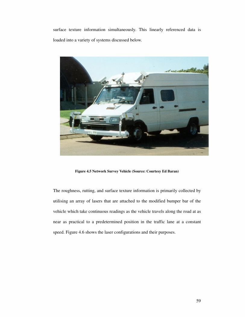
59
surface texture information simultaneously. This linearly referenced data is
loaded into a variety of systems discussed below.
Figure 4.5 Network Survey Vehicle (Source: Courtesy Ed Baran)
The roughness, rutting, and surface texture information is primarily collected by
utilising an array of lasers that are attached to the modified bumper bar of the
vehicle which take continuous readings as the vehicle travels along the road at as
near as practical to a predetermined position in the traffic lane at a constant
speed. Figure 4.6 shows the laser configurations and their purposes.

60
Figure 4.6: Network Survey Vehicle Laser Array Configuration
(Source: Courtesy: Ed Baran)
Roughness is a measure of the longitudinal profile of a road surface and is
reported against the International Roughness Index (IRI). Roughness is captured
by measuring the comparative rate of change in height between readings along
each lasers path. This information is correlated to determine how many times the
rate of change would result in a certain amount of movement in a vehicle
suspension. Each time the amount of movement is exceeded a count is added
which varies based on the magnitude of the movement. This information is
summated into an average value for each 100 metre section of roadway.

61
Additionally data is also collected by mechanical means using a roughness tower.
This data is utilised as a check on the accuracy of the laser data and as a back –
up, should there be an apparent error in the laser data. Potential sources of error
in the roughness data include Tdist related, vehicle tracking errors where the
vehicle may drift from the desired optimum position, loss of laser signal
(generally for a short section only), and limitations of the equipment. For the
purposes of this project the primary focus is on the outer wheel path roughness as
this correlates with the road position that the skid resistance data was captured
on. It is acknowledged that roughness is a factor in skid resistance as high
roughness road sections may result in loss of contact between tyre and pavement
thereby resulting in a decrease in available skid resistance. Additionally the
roughness parameter provides another guide to general pavement condition and
therefore aids as supporting information in the prioritisation process.
Significant analysis tools already exist to identify and prioritise sections of
roadway that exhibit high roughness. It should be noted that roads that exhibit
high roughness are problematic for the skid testing equipment due to the
inconsistencies they cause between the test wheel and pavement surface. Much
of the variability in skid test results and need for retesting is a result of roughness
related issues.
Rutting is a deformation of the pavement that occurs in the wheel paths resulting
in a linear depression along the road. Rut filling operations over the past several
years of those areas approaching the treatment intervention levels mean that
rutting is not significant in the test areas. For this reason rutting will not be

62
considered further for the purposes of this project. One observation made during
the initial examinations was that in rut filled areas there was a substantial
decrease in the surface texture depth. This may affect the macrotexture available
for drainage although this has not resulted in any apparent issues to date it will be
monitored.
Surface texture for this project utilised the Sand Patch Test Equivalent value for
the outer wheel path (OWP) extracted from ARMIS. The Sand Patch Test
involves the placement of a defined volume of sand on the pavement surface.
The sand is spread across the pavement in a circular shape until all the voids in
the pavement are full and the top level of the sand forms a flush level with the
aggregate. The diameter of the circle is then measured with the texture depth
being equal to the volume of sand divided by the area the sand covered. This
parameter is captured utilising profiles obtained across the pavement with the
laser array. As the resultant laser measurement is not a true measure of surface
texture depth Main Roads has adopted a relationship between the two which is
calculated by multiplying the laser measurement by 2.5.
Adequate surface texture is required to ensure that there is sufficient
macrotexture to allow water to drain from a pavement thereby preventing
aquaplaning. For the purposes of this project adequate texture depths were
adopted based on seal type. Minimum surface texture depths of 1.0 millimetre for
chip seals and 0.4 millimetres for asphalt surfacing were adopted based on
AUSTROADS guidelines. In sections of asphalt where readings of 0.6
millimetres or less were found the depth was considered adequate but noted as

63
marginal. As such where other factors also proved inadequate this parameter was
used to aid in prioritisation. Flushed or slick pavements generally exhibit a low
surface texture depth. Sources of error include Tdist related, vehicle tracking
errors where the vehicle may drift from the desired optimum position, loss of
laser signal (generally for a short section only), and limitations of the equipment.
Another important factor that surface texture depth provides to the picture of
pavement performance is achieved through the comparison of the depths
recorded between the wheel paths (BWP) and for the inner wheel path (IWP).
Where readings between the OWP and / or IWP are considerably different than
those recorded at the BWP position this may indicate a structural issue with the
underlying pavement. That is, the loads on the trafficked parts of the surface have
affected its profile compared to the unloaded areas. This may be visually
confirmed via evidence of stones impaction, flushing, or rutting.
Accident information is collated in the Roadcrash 2 database. This database
contains a wide range of data on individual accidents on the road network. Each
crash record includes details of the road number, locality description, severity,
contributing circumstances, vehicles involved, weather, time of day, type of
accident and a textural description to name a few. The quality of this data varies
considerably in completeness, positional accuracy, and detail and as such is only
useful to determine trends and possible problem areas that require further
investigation. A key priority on the reception of the skid deficiency data was the
examination of individual crashes specifically targeting any correlations between
skid deficient sections and crash rates. It would be expected that the accident risk
64
would increase as the skid resistance decreased. A Black Spot criteria analysis
was also undertaken utilising 1 kilometre sections and a 250 metre radius around
intersections for accidents over the past 5 years.
The Traffic Analysis and Reporting System (TARS) is the departmentally
developed source of the average annual daily traffic information (AADT) for
road sections. It has been shown that heavy vehicles have the most impact on
stone polishing (Oliver, 2002). However for the purposes of this analysis the mix
of commercial vehicles (trucks) and cars is not investigated. It is likely however
that where specific detailed investigations of areas identified through this process
are carried out that this is a likely factor for analysis. This project will utilise
AADT purely as a statistical measure. AADT also provides input into the TARP
analysis process which uses the AADT to establish crash rates per vehicle
kilometre travelled. Possible sources of error in the TARS data include, field data
collection errors, equipment failure, processing errors and abnormal events
affecting data collection and resultant output accuracy.
4.4 Spatial Data
A wide range of relevant spatial data is available in the District for integration
and enhancement of map presentation. This data is stored centrally on the district
server and utilises a structured directory approach to group similar datasets
together. This data is currently obtained through a variety of sources including
the Departments’ Geospatial Technologies Branch, Roads Information Branch,
various web servers, through field collection by District staff, and in some cases

65
from local groups or organisations. Data is generally obtained in Mapinfo format.
A typical example of metadata that is kept on datasets, giving accuracy, currency,
and a myriad of other information, is the DCDB dataset which has been included
in Appendix C of this dissertation.
Reference systems utilised for this and all other projects within Mackay District
Main Roads include:
• Geocentric Datum of Australia 94 (GDA94) – horizontal reference
system; and
• Australian Height Datum (AHD) – vertical reference system
This approach to reference management allows consistent integration of datasets.
Key datasets utilised in the delivery of this project include, with the dataset name
listed in brackets:
• State Controlled Road Centrelines (sc_roads) which consists of a state
wide set of Main Roads controlled roads.
• State Digital Road Network (allroads) which consists of all road
centrelines within the Mackay District. This dataset was utilised to assist
the end user to visualise a location once the map is zoomed into an area
of less than 10 kilometres.
• Digital Cadastre Database (DCDB) which consists of all land parcels,
casements and easements within Mackay District. This data is comprised
of many smaller datasets that cover each of the six Local Authority Areas.
This data is set to display once a zoom level of 10 kilometres has been
reached to aid in visualisation of a location.

66
• Queensland Coastline (Coast) is a representation of the coastline that aids
in the visualisation and presentation of the map product
• Queensland Towns (Towns) is a representation of the named towns within
the study area. This state wide dataset has been manipulated such that
only major towns have been displayed.
• Ocean is purely included as a cosmetic layer to enhance presentation and
is a derivation of the Coastline dataset used to represent the ocean.
• Queensland Local Authority (lga) boundaries dataset depicts the location
of local authority boundaries across the state.
4.5 Digital Video Road
As previously discussed the network survey vehicles capture digital video images
of the network as part of the annual road pavement condition testing program.
For the sealed road network a four camera system is used that provides images of
the road and features in the forward and reverse directions and left and right sides
of the vehicle (Figure 4.7). This data is provided to the district in the form of a
series of images at intervals of 10 metres along each road section. The data is
placed on the district server and is accessed from individual personal computers
by utilising a Digital Video Road Viewer. These videos provide valuable
information about the nature of the pavement surface condition, asset locations,
signage, and the general environment that a section of road exists in. This can be
very useful in the preliminary investigation and identification of possible
problem areas for a wide range of Main Roads activities. DVR also facilitates

67
enhanced communication of issues through improved visualisation and provides
a useful auditing tool.
Figure 4.7: Digital Video Road Viewer (Source Department of Main Roads, Mackay)
For the project this system was used in the subjective assessment of possible
problem areas and as a confirmation tool for perceived problems. Problems
identified using a wide range of information could then be field inspected with
confidence that a significant issue exists at the location rather than relying on
perception thus reducing potentially wasted resources by inspecting areas
identified due to erroneous data.
The incorporation of a dynamic link between DVR, GIS and other systems such
as Chartview such that they may be viewed simultaneously is an additional
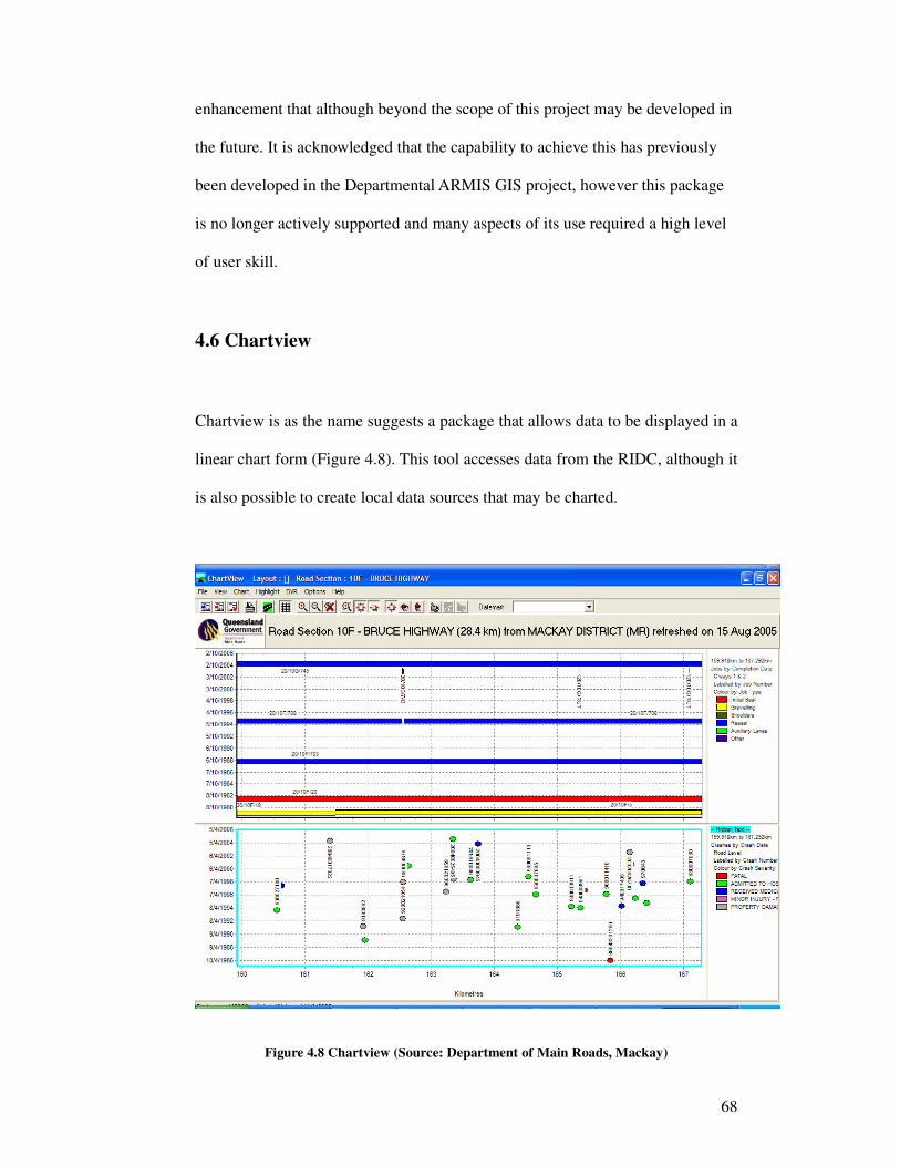
68
enhancement that although beyond the scope of this project may be developed in
the future. It is acknowledged that the capability to achieve this has previously
been developed in the Departmental ARMIS GIS project, however this package
is no longer actively supported and many aspects of its use required a high level
of user skill.
4.6 Chartview
Chartview is as the name suggests a package that allows data to be displayed in a
linear chart form (Figure 4.8). This tool accesses data from the RIDC, although it
is also possible to create local data sources that may be charted.
Figure 4.8 Chartview (Source: Department of Main Roads, Mackay)

69
Chartview was utilised as a visualisation tool in the subjective aspects of the
assessment to confirm relationships between various factors. In the future this
tool could be dynamically linked to the GIS system to further enhance
communication of issues. Chartview already has a dynamic link established with
DVR which enables simultaneous viewing. Chartview may be viewed as a
graphical display of the data that allows relationships to be established between
various features of the road network, but does not have the capability to allow the
completely integrated association of the surrounding environment that can be
achieved through a GIS. Chartview was utilised in this project to aid in quick
assessment of pavement parameters.
4.7 Databrowser and other tools
Several other tools were utilised to access data and carry out assessments and
each is now discussed.
Oracle Databrowser is a database querying tool utilised to link (join), query,
export, and report data tables contained within ARMIS. Much of the data within
ARMIS that was required for this project was stored in a wide range of Oracle
based tables that had to be brought together into a usable format.
Mapview is a departmental add-on application to MapInfo. It is useful in the
display of maps of ARMIS data which it sources from the Roads Information
Data Centre (RIDC). The RIDC contains a selection of data parameters from the
parent ARMIS systems, but does not contain the complete dataset. Other datasets

70
are able to be associated with the resultant map product. For this project various
datasets have been merged and information added and as such this environment
does not offer an advantage. However, once the methodology for assessment has
been established this system may be utilised to deliver future evaluations.
4.8 GIS Software
Geographic Information Systems (GIS) are a powerful set of tools that facilitate
the capture, input, data management (storage and retrieval), manipulation and
analysis, and outputting of geographical data. Geographical data may be
described as data about an objects’ spatial position relative to a known reference
system, its relationship to other objects around it, and its associated physical
attributes.
The GIS package utilised for this project is MapInfo Professional Version 7.5
which is a desktop level mapping application. This package provides the level of
functionality required for this project in a user friendly manner and is currently
widely available across Main Roads through an unlimited usage corporate
licensing agreement. Over a period of time Main Roads has developed a series of
tools to assist in the use of MapInfo for departmental needs. These tools written
in MapBasic are collectively known as the “Nerang Applications” in recognition
of the District where the majority were developed.
The Nerang Applications greatly improve the access to the systems by a wide
range of people with varying amounts of knowledge of GIS through facilitation

71
of a very user friendly intuitive environment. The applications range from those
which facilitate tracking of land developments through to simple road centreline
queries. The applications also facilitate the development and use of standard
workspaces through a menu and layer control system that avoids the need for the
end user to have a full knowledge of GIS. This is particularly useful for managers
who with the click of several buttons can easily find the answer to basic queries.
This project makes extensive use of the Nerang Applications to enable a user
friendly environment. Applications extensively utilised include Road Centreline
Tools, Workspace Layer Control, and Menu Control. GIS offers an ability to
query and interrogate spatial and statistical data based on user defined scenarios
which may aid in decision making processes. The power of GIS as a data
integrator, analysing and presentation tool all make it an ideal choice for this
project.
4.9 Prioritisation Software
As previously discussed Scenario Millennium is the current departmental
pavement management system for the identification, development, prioritisation,
and management of pavements. However, Scenario Millennium does not
consider additional aspects such as skid resistance when looking at the pavement
performance. This project aims to bring the various aspects that are considered
into a more inclusive environment. Although software development is beyond the
intended scope of this project the development of methodologies that has
occurred may be used in the future development or enhancement of existing

72
systems. A key aspect of this project is the establishment of the nature of
relationships between skid resistance and other pavement parameters. Only with
this knowledge can informed decisions be made on the significance of the skid
data in the prioritisation process. That is, it may be found that other aspects of the
pavement trigger intervention prior to skid resistance becoming a factor. In any
case it is likely that skid resistance data will give added support to competing
sections of pavement in the prioritisation process. Skid resistance data is also
likely to assist in identifying non performing aggregates, construction practices
and treatments resulting in improved efficiency and effectiveness in the delivery
of the road network to the people of Queensland.
4.10 Conclusion
To deliver the most appropriate road asset management solutions the Department
needs to ensure that it considers a wide range of factors including skid resistance
in the evaluation, planning, construction and maintenance of the network in a
timely manner. The pavement is a key component of the road asset and
represents a significant investment of resources.
Various tools exist to assist the Department to prioritise and evaluate what is
required of the road asset. In terms of pavement management the departmentally
developed Scenario Millennium represents a significant package through which
effective decision making support is provided. However this system does not
currently encompass all aspects required of a pavement management system with
skid resistance being one of these areas. Scenario Millennium is a decision

73
support tool which provides input through the identification, development,
prioritisation, and management of pavements for the maintenance programs. Like
many decision support tools Scenario Millennium is only as good as the data
input it receives with many possible sources of error and therefore outcomes
derived from the software must be validated by field inspection and the use of
engineering judgement.
Skid resistance data was captured by the Pavement Testing Unit of the
Department using a Norsemeter ROAR Skid testing device. The area chosen
consisted of a variety of road classes and environments totalling 978.3
kilometres. The report received after the testing indicated that 16% of National
Highway and 11% of other roads recorded levels below the relevant investigatory
levels and require further investigation. Investigatory levels for skid resistance
have been established however a methodology that is able to be consistently
applied to assess the identified areas is yet to be developed. This is one of the
primary aims of this project. The methodology that has been developed will
facilitate the prioritisation and management of skid resistance whilst considering
other pavement condition parameters across the district network.
The Department collects a wide range of asset information annually to enable
effective management of the road asset. The majority of this information is
collated in the ARMIS group of systems which include provisions for the entry,
storage, auditing, manipulation, editing, and reporting of this data in a variety of
formats. The data utilised for the project is of variable quality and as such a
purely desktop solution is not achievable. The spatial datasets utilised in this

74
project were sourced from a wide range of agencies in a MapInfo format.
Appropriate metadata detailing ownership, custodianship, accuracy and currency
is kept for each dataset. Other departmental systems were utilised to confirm
various aspects of the assessment including Databrowser, MapView, Digital
Video Road and Chartview.
MapInfo Professional Version 7.5 was utilised to deliver this project. Mapinfo
has developed a programming language known as MapBasic that facilitates
development and delivery of software to meet custom application needs. Main
Roads has developed a series of customisations collectively known as the
‘Nerang Applications’ to enhance user friendliness of the system. Several of
these customised applications were utilised in the delivery of this project.
A key aim and objective of this project is the development of an appropriate
methodology through which skid resistance is able to be prioritised and managed
efficiently and effectively in relation to overall pavement management strategies.
An additional outcome may be contribution towards confirming the appropriate
service life of particular pavement types in each environment.

75
CHAPTER 5 METHODOLOGY & ANALYSIS
5.1 Introduction
Road asset management is a very complex issue due to the wide range of factors
that need consideration in deciding how to best allocate limited resources. It is
vital to gain a "big picture" view of the entire network and the impact that each
factor has on it and the relationships and any trends that may exist between them.
As much of the data is in digital form it is logical that decision support tools be
developed in a computer based environment that assist the Department to
discharge its obligations in an effective and efficient manner.
There are many different approaches and systems available to the asset manager
that may be used to analyse information, support decisions and identify priority
areas for investigation. However, currently none of these provide a complete
solution that identifies and takes into account all the possible factors that may or
may not affect a given situation. The GIS environment with its ability to integrate
a wide range of data lends itself to situations that involve complex issues such as

76
this. It is emphasised that as with all data management and analysis systems the
properties of the underlying data must be understood. In the case of pavement
management assessment the results of analysis by computer systems should
never be taken as certain or complete, but rather as a guide which is based on a
series of factors at a given time. The priorities that are developed from these
systems value is identification and highlighting of particular areas that appear to
require further investigation and / or possible treatment. A purely desktop based
solution is not advisable because if the analysis is based on poor or incorrect data
the prioritisation will be incorrect. Thus it is essential that the other components
of field inspection, technical knowledge and stakeholder involvement are utilised
in the ultimate decision making process. As this was the first time skid related
data had been collected it was essential that a clear picture of the issue on the
district network was gained as only through knowledge can informed
management occur.
5.2 Procedure
Although this project involves use of a diverse range of queries and analysis
techniques several key generic processes are common across the project (Figure
5.1). It should be noted that some analysis undertaken builds on the results of
other queries so some aspects of this procedure may not apply to each process.
Generally where such processes occurred they are notated in the relevant section.
This approach to the system management process facilitates construction of a
controlled and reliable environment that allows efficient and effective delivery
and investigation of road information.

77
Start
Collation of Data
Data Review, Reformatting and Manipulation
Geocode data
Build Workspace
Generate Queries and Analysis
Develop Menu
Develop Layer Control Buttons
Reporting Formats and Presentation
Test Outputs
Ends
Figure 5.1 Procedure for Skid Resistance Evaluation System

78
The development of this system will enhance the communication and
understanding of skid resistance issues in Mackay District. The GIS interface
developed will allow non specialist GIS staff to access, interrogate, and evaluate
a multitude of parameters and effects that skid resistance has on the District
network. The analysis derived from this system will enable resources to be
focussed on those areas that require priority inspection and provide staff with a
clear view of what areas of the general issues faced in the road environment. This
enhanced knowledge will in turn lead to a fuller understanding of issues, their
effects and facilitate the development of a more rounded view of these issues.
Such an approach should lead to a more informed decision making process and
consequently a more effective and efficient placement of resources.
The 'Nerang Applications' has the capability to create menu items that appear as
a drop down list in MapInfo. This provides users with easy access to core pre-
built workspaces such as this one in addition to various spatial datasets, data
capture tools, data maintenance facilities, spatial navigation engines, and
facilitates the creation of high quality maps. Several 'Nerang Applications' were
involved during the development of this project and will continue to be utilised
during operational phases of the system. Applications utilised include the Road
Centreline Tool, Workspace Manager, Menu and Layer Control Tools, Graphic
Tool, and Hotlink Tool. Other documents, images and plans use the 'Hotlink' and
Graphic tools in MapInfo, to enable the user access to additional information on
each road section.

79
5.2.1 Initial Investigations
Initial investigations through inspection of various datasets indicated that the
majority of the possibly deficient sections were nearing the end of their expected
seal design life. Many of these aged sections exhibit sufficient surface texture
depths (macrotexture) within AUSTROADS Guidelines (2003) so it is likely that
the skid resistance issues are related to the in service polishing of the aggregate
by traffic. Polishing has the effect of reducing microtexture and therefore the
available friction. This provided a focus for further investigation.
Several methodologies were utilised to examine the data. These were based on
firstly satisfying any issues that the testing identified that necessitated immediate
actions, secondly on establishing underlying causation and relationships between
skid resistance and other pavement parameters, and thirdly on development of
methodologies and strategies to efficiently and effectively investigate, monitor
and manage skid resistance. It is emphasised that many of the datasets utilised in
this process are of variable quality, completeness and contain aspects that are the
result of subjective assessment. As such the desktop solutions presented should
be used as a guide to focus investigatory effort. The final decision making
processes and prioritisation will include field inspection and engineering
technical advice.
5.2.2 Obtaining Information
The majority of information utilised for this project was already held in a variety
of systems within Mackay District. However considerable amounts of data

80
required reformatting to enable it to be spatially enabled, ensure completeness
and ensure that its useability was maximised. Typically this involved addition of
columns that contained subjective data or positional information. A typical
example using Seal age data where an adjusted seal age has been calculated is
shown in Figure 5.2.
Figure 5.2: Additional Columns added to Seal Age dataset
Almost all the pavement related datasets required some manipulation. This
primarily involved the reduction of the broader datasets to the same geographical
extents and in some cases the addition of some fields to make manipulation and

81
querying easier. Where subjective data was added this was often the result of a
lengthy process of evaluation.
It is important to note that the data contained in many of the parent systems is
imperfect, in some cases of low quality or incomplete and for this reason a high
degree of subjective assessment, inspection and local knowledge of the network
is required for the development of appropriate priorities. In the majority of cases
the data is captured in one traffic lane only and has been assumed to be similar
for adjacent untested lanes. This assumption may not be universally valid and
hence further detailed analysis is required of sections that involve such lanes.
5.2.3 Review and Evaluation of Information
It is vital to review and evaluate the data to be utilised in any project as the
outcomes are likely to be incorrect should the data be inappropriate for the
proposed usage. If data is deemed unreliable it is vital that the limitations of
outcomes of analysis be clearly stated as a minimum. If a wide range of data is
to be integrated the best way to manage this must be established so that the final
product is unambiguous and clear in its communication of outcomes. For this
project given that the individual datasets are accessible using a range of other
methods and systems external to the project control is not entirely possible.
Metadata does provide a solution where data is accessed from individual
systems. However where combinatorial operations are utilised this becomes
problematic. For this reason a warning is provided in the form of a statement
within the legend of output information stating the following. ‘The data

82
displayed on this map is provided as a depiction that may not represent the true
physical relationships between features. The depiction is a representation of the
source data and requires confirmation by field inspection. Please contact your
GIS Officer for further information.’
An assessment was also undertaken of any likely sources of error that may exist
in the data so that effects could be understood and taken into account when
developing an analysis approach. Metadata provided a valuable source of
information in the investigation of this aspect.
5.2.4 Data Creation Processes
This project required examination of a wide range of parameters and data
relationships so their effects on the road network and its usage could be
established. Some of these areas requiring investigation arose from reports and
related departmental initiatives such as Barans' (2004) report which suggested
aggregate properties required investigation as a possible source of skid
deficiency in the District and North Queensland Regions' approach to meeting
the requirements of the Road System Manager framework. In addition to
examining these issues an investigation into broader trends and relationships
between pavement performance parameters such as seal age verses skid
resistance properties, and asphalt verses chip seal was warranted. Firstly, an
approach to analyse the data to establish any relationships with accidents was
required. It is emphasised that when accidents occur where the road appears to be
a factor that they are and have always been investigated promptly.

83
The North Queensland Regions' Strategic Directions 2004-2005 Policy document
identifies Deficient Skid Resistance as element 29 of its strategy to meet the
requirements of the Departmental Road System Manager framework. An
assessment of wet weather accidents is undertaken as part of this strategy. Wet
weather accidents are considered more likely to occur where there is a skid
deficiency present. In Mackay District there were several approaches taken to
examine the different aspects of the skid resistance / accident relationship.
Two datasets in particular required considerable development and a range of
additional information. Both these datasets established relationships between
road crash information and the skid deficiency testing and are now discussed.
5.2.4.1 Wet Road Crashes Table
Wet road conditions are considered to be more likely than dry conditions to show
skid deficiencies in road pavement as water results in a reduction in the available
friction. This dataset was an extraction of data from the Departments RoadCrash
2 system and contained various details of road accidents that occurred between 1
January 2000 and 30 March 2005. It was decided that due to the uncertainty of
the nature and amount of additional data required that this base table would be
built in Microsoft Excel with the final product being mapped, integrated and
analysed in the GIS environment.
1. The table was initially filtered in Excel to remove crashes that occurred in
dry weather conditions and sorted so that the severity of crashes were

84
grouped with the most serious at the top of the table. Unknown and Fog
condition accidents were also retained for consideration as they may have
occurred in wet conditions. The following factors were then assessed and
results recorded in the table;
2. Review all police accident reports of the wet crashes to establish whether
skidding was a contributory factor in the accident. The accident reports
are sourced through Roadcrash 2. Note also any mention of water on or
over road which may indicate a pavement drainage issue;
3. Identify whether the accident had occurred on a possibly skid deficient
section or not. This was completed by firstly querying the Wet Crashes
dataset using Structured Query Language (SQL) in MapInfo to select
those accidents where skidding appeared to be a factor (Figure 5.3) This
operation is a typical example of an SQL query used in the delivery of
this project.
Figure 5.3: Query of WetRoadCrashes dataset

85
4. An Intersection operation using SQL was then carried out to establish
which of these accidents fell on the skid deficient road sections;
5. Identify whether the accident occurred on Asphalt or Chip Seal through
examination of the pavement layer information contained within ARMIS;
6. Identify whether the accident occurred where sufficient texture depth
existed. This data used the assumption that a minimum surface texture
depth of 1 mm was required for chip seals and 0.4 mm was required for
asphalt surfaces. It is acknowledged that in the case of high demand
asphalt pavements that 0.6 millimetres may be a more appropriate
minimum surface texture depth, however for this analysis these
AUSTROADS guidelines were adopted as an initial starting point. Where
values were close to these levels they were notated in the comments
sections of the table;
7. Investigate whether the site was treated post accident through
examination of Chartview. By comparing completion dates of jobs
against accident dates treatments that have occurred post accident can be
identified;
8. View Digital Video Road to establish any visual factors and confirm
pavement condition Aspects targeted included evidence of flushing,
rutting, cracking, stone loss and pavement deformation.;
9. Comment on any issues identified and whether any initial action may be
required. This allows a quick search of those areas that may require a
treatment. It includes areas that are already programmed for treatment,
which are included as requiring action as they are yet to occur;

86
10. Identify any apparent accident clusters. Generally a 250 metre radius
around intersections was utilised whilst most mid block or non
intersection road sections were considered based on homogeneous
sections. The majority of mid block sections were less than 500 metres
long. This work was carried out primarily in the Excel spreadsheet
environment through the use of sorting routines, however was also
visually confirmed using the GIS environment. It is acknowledged that
this operation may have been carried out solely within the GIS
environment using proximity analysis however there was a considerable
degree of subjectivity in the assessment and the Excel spreadsheet
allowed the result to be delivered within a few seconds. In this case GIS
was used to confirm and visualise the analysis carried out in Excel. This
analysis included both skid related and non – skid related wet accidents.
Each of these clusters is viewed as a priority area for investigation; and
11. This table was subsequently geocoded to allow integration, analysis and
display with other datasets.
5.2.4.2 Inspection Priorities Table
The second dataset was constructed as a collation of information from various
sources again using the Excel environment. The resultant table was based on an
extraction from the skid resistance report supplied to the District. The
methodology involved an initial assessment of the skid resistance data. The
priority in this process was to establish whether there were any skid related
accidents occurring on the possibly skid deficient sections. This assessment used

87
a similar premise to that developed in Northern Regions' Strategic Directions
2004 – 2005 document. Construction of this table involved the following steps;
1. Selection of those sections from the test report where the probability of
failure to meet the skid investigatory levels was greater than 30% using
Excel;
2. Run the Roadcrash2 TARP crash analysis of the entire District road
network spanning the last 5 year period with parameters of 250 metre
radius around intersections and 1 kilometre road sections. The outcome of
this analysis is a report that ranks locations based on a complex formula
that considers the cost of the crashes involved, crash rate at location per
vehicles that use the location, and the relative rate that the location has
compared with the rest of that road section. The analysis reports in terms
of an actual crash rate compared to a critical crash rate. Where the
relationship results in a positive value the crash rate at the location is
identified as higher than normal. This report was procured in a hard copy
format. For the purpose of this analysis these locations were described as
blackspots. Those blackspot sections that fall in a possibly skid deficient
section are notated in the spreadsheet. The specific locale of the blackspot
section within the specific possibly skid deficient section was also
identified to aid in prioritisation in an adjacent column of the spreadsheet;
3. Identify any apparent skid related accidents in the possibly skid deficient
road sections. This data was obtained from the Wet Road Crash
assessment carried out above and notated in the spreadsheet;

88
4. Determine seal age and notate for each possibly skid deficient section in
the spreadsheet. This data was extracted from the Seal Age dataset which
contained adjusted dates to match the testing;
5. Using the resultant table from step 1 input additional location data and
other fields in the spreadsheet. Fields entered included a local area
description, through distance start and length fields. These aid in end user
understanding of the individual section and also form part of the
reformatting preparation process for MapInfo geocoding;
6. Identify whether each section has adequate or inadequate surface texture
depth. As with the wet crashes table this data applied the same
assumption of required minimum surface texture depth. The same
notation and commenting process used in the wet crashes table was also
utilised;
7. Identify and notate any programmed treatments for each of the sections
through examination of proposed works programs;
8. Notate comments on these parameters. This includes validation and
comments on any of the data described in other columns. For example
barely adequate texture depth may be commented;
9. View Digital Video Road to establish any visual factors and confirm
pavement condition Aspects targeted included evidence of flushing,
rutting, cracking, stone loss and pavement deformation;
10. Prioritise locations based on the following criteria. Obviously all
priorities have possibly skid deficient pavement in common;

89
a. Priority 1.
i. Includes a Blackspot section which indicates a higher than
normal crash rate for that environment; and
ii. Evidence of 1 or more skid related accidents
b. Priority 2.
i. Includes areas where EITHER a Blackspot section has
been identified or 1 or more skid related accidents have
occurred.
c. Priority 3.
i. Possibly skid deficient areas that do not have a Blackspot
section but may have a skid related accident identified that
are in the design phase. These areas may also have other
pavement deficiencies in addition to possible skid
deficiency.
d. Priority 4
i. Possible skid resistance deficiency was the only significant
pavement defect identified at the site. Close monitoring of
the site is suggested.
11. Notate reasoning for priorities. This provides a place for validation of
initial decisions to be accommodated;
12. Immediately inspect priority 1 sites that have not already been addressed.
This process is repeated for all the identified sites in an order of
decreasing priority;
13. Report findings with recommended actions;
14. Program remedial works;

90
15. Monitor performance of treatment solution. It is emphasised that
resealing is not necessarily the solution; and
16. This table was also subsequently geocoded to allow further integration,
analysis and display with other datasets.
It is acknowledged that several of the steps involved in the construction of these
tables may have been carried out by other means however this approach will
allow greater ease in querying and smoother data integration.
5.2.5 Geocoding Information
Information was geocoded utilising the 'Nerang Applications' geocoding wizard
which forms part of the Road Centreline Tools. This tool utilises the state
controlled road network centrelines, road identification number, Tdist and length
to produce graphical representations of features on the network. Appendix G
contains an example of the AADT dataset being geocoded. Tables were geocoded
utilising this tool for all the ARMIS related and derived datasets for this project
utilising this tool.
5.2.6 Creating a MapInfo Workspace
Once the various datasets have been collated, and manipulated into an
appropriate format and subsequently geocoded against the road centreline the
integration of data can commence. This is achieved by the construction of a
workspace. A workspace may be likened to a cooking recipe. The workspace tells

91
the computer what ingredients are required, in this case the ingredients are
datasets, where those datasets are located, how it wants them displayed, and the
order it wants them displayed to produce the desired output. Datasets required for
this project include DCDB, road networks, coastline, various road pavement
related datasets, DVR, towns, hydrology, and Local Authority Boundary
information.
Appendix D provides an image of some of the various datasets that form
individual data layers utilised in this project through the use of the MapInfo
Layer Control dialog. Additional to the base data layers, various thematic map
layers are also present in the above Layer Control image. A thematic map is a
layer generated from a dataset based on a particular theme. Appendix E displays
the Legend Window from one such thematic layer.
MapInfo provides a full range of zooming, panning and related tools and the user
is able to associate additional data to that included in the workspace should they
so wish. This flexibility in approach and data integration is the strength of the
GIS environment.
5.2.7 Customise the ‘Main Roads’ Menu
One of the advantages of the Departments 'Nerang Applications' is the ability to
develop menus that are accessible to all users in the district. This facilitates the
easy development and distribution of pre-built workspaces for commonly used
activities and tasks. This approach also enhances accessibility to basic maps for

92
non technical staff usage. Figure 5.4 below shows an example of the Main Roads
Menu including the Skid Resistance workspace link.
Figure 5.4 Main Roads Menu including Skid Resistance link
Appendix F shows the dialog utilised in setting up the menu link utilising the
Main Roads Menu Administration component of the 'Nerang Applications'. Note
that this area also allows a variety of other 'Nerang Applications' to be
automatically opened when the link on the menu is triggered by the end user.
This feature has allowance for any MapBasic application to be automatically run
as part of the opening of the workspace and therefore enables non technical end
users to access the complete user interface without necessarily having an intimate
knowledge of the technology or applications involved.

93
5.2.8 Layer Control Utility
It is likely to be unclear to a general user what each particular dataset may relate
to based on its title. Whilst metadata is utilised to clarify this, an additional way
to achieve this is by grouping layers together based on their topic. For example,
if all land parcels are grouped together under a group entitled cadastre then the
end user does not require a detailed understanding of the individual dataset layer
titles that make up this group.
The 'Nerang Applications' include such a layer grouping functionality. The
Workspace Layer Control Tool allows a meaningful grouping of similar themed
tables. The tool creates a radio button pad which loads with the workspace and
allows a toggle on or off display of each group (Figure 5.5). Individual buttons
each have an icon that gives a visual cue to the subject they pertain to as well has
an attached help string which facilitates a bubble display giving a textural
description when the user places the mouse over it.
Figure 5.5 Workspace Layer Control
Appendix H contains an image of the layer control tool dialog used to develop
the layer control pad for the Skid Resistance workspace.

94
5.2.9 Representation of Information
Establishment of the best way to display each dataset such that any confusion
between differing features is avoided and communication of the significant issues
is enhanced is a vital aspect of any GIS project. In this project there was a large
amount of information involved that was linearly referenced over the same
geographical extents along a network of geographical objects. This presents a
significant challenge as the project is dealing with a multi facetted parameter
where a wide range of relationships were sought to be investigated and reported.
The approach taken was to utilise a combination of analysis techniques and
display options to ensure that communication of desired attributes was clear and
effective. This was achieved in the following ways.
1. The use of zoom controlled layering. This means that certain larger
datasets are not visible to the end user until a certain zoom level is
reached. This allows avoidance of unnecessary clutter that detracts from
the depiction of the desired features.
2. The use of Workspace Layer Control. This is a tool that was a
departmentally developed as part of the "Nerang Applications". The tool
allows the grouping together of similar tables of data under a series of
theme based toggle buttons. This allows the user to chose which groups
they want displayed without an in depth knowledge of the data tables.
Similar buttons have been constructed for likely queries so that the user
only need select the appropriate button to gain a visual representation of

95
the desired dataset or combination of datasets. Each button that forms
part of the layer control has a help bubble attached which displays when
the mouse is passed over it and describes what feature the button
pertains to.
3. Creation of Thematic Maps and Symbology. This project involved many
datasets which covered the same approximate extents and this creates
challenges in ensuring a meaningful display of the desired attributes.
Whilst this could largely be controlled by the workspace layer control
there are a lot of cases where combinatorial mapping of features was
required. An additional challenge was the large size of the area that the
project encompassed which was further complicated by the linear nature
of the network along which the features were being mapped. In addition
to the workspace layer control the use of colours and line styles to
accentuate features of importance was utilised. A variety of analysis
techniques were utilised including thematic mapping. Thematic mapping
is mapping of a particular theme. Thematic mapping was utilised on
most datasets and queries to highlight the key attributes. A legend
detailing symbology is naturally also provided to ensure comprehension
of the display.
4. Printing Tools. The "Nerang Applications" also include a tool that
allows a basic printing layout which title, logo, legend, north point, scale
bar, title and footnotes to be created. End users have been instructed in
the use of this tool. The Skid Resistance Assessment application is
designed for an interactive digital environment rather than a hard copy
format. Generally end users will view small sections of the network

96
individually rather than the entire network. For this project it was not
practical to produce a complete map as the features and their
relationships would not be viewable at an appropriate scale. Maps can
be produced over smaller extents quickly and easily through the use of
the mapping tool.
A future enhancement of this approach would be delivered through the ability to
create sub menus. The above processes mean that the end user gains a clear
understanding of the particular aspect of the project that they are interested in.
5.2.10 Data and Statistical Analysis Outcomes
The focus of this dissertation now shifts to the outcomes realised from the
analysis of the tables. Particular focus is given to the relationships established
through the wet crashes and inspection priorities tables. Additional associations
between various pavement parameters are then discussed.
5.2.10.1 Wet Road Crash Table Analysis and Comments
1. A total of 1998 accidents occurred on the District network between 1
January 2000 and 31 March 2005. This dataset once reduced to those
accidents that occurred in wet, foggy or unknown conditions contained
296 accidents. It is acknowledged that this selection may be imperfect as
water can be a factor on the roadway due to factors other than rain such
as overflow from sprinklers watering grass islands or incorrect

97
documentation in the police report. In Mackay there are few locations
where such irrigation is in place. The assumption was made that the vast
majority of relevant accidents will be correctly identified. Of these
accidents 47% resulted in property damage only.
2. Of the 296 wet accidents 166 appeared to have a skidding factor. It is
emphasised that this number includes accidents that would have still
occurred irrespective of the amount of available skid resistance such as
accidents involving disobeying traffic lights or driver distraction. These
were included because although the driver was considered the primary
causation they still had attempted to brake. Factors that resulted in
exclusion included non skid accidents involving driver fatigue, driving
under the influence (DUI), and other unusual incidents. It is also
acknowledged that accidents generally occur due to multiple factors. It is
significant that the severity outcomes of an accident may vary depending
on the skid resistance available (Oliver, 2002).
3. A selection query of the Wet Road Crashes table within MapInfo was
carried out to establish the number of accident reports that mention water
on or over the road surface. This resulted in 32 accidents being identified
at 25 locations. These sites and in particular those that occurred where
there were a cluster of accidents were immediately inspected with
remedial action proposed where appropriate. Nine of these sites had been
treated since the accident occurred. Interestingly only one of these
accident sites was identified as having occurred on a possibly skid
deficient pavement. These accidents while significant in terms of safety
are a reflection of pavement drainage issues rather than skid issues.

98
Whilst this was not an initially sought attribute of this project the review
process allowed easy identification of such issues as an additional benefit
and is an example of the proactive approach to the management of
pavement related issues that the District is taking.
4. In the construction of the Wet Crashes dataset it was noted whether the
road section had been treated since the accident had occurred.
Examination indicated 42 of the 166 skid related accident sites had been
treated since the accident. On face value this may seem poor but it is
critical to understand that the majority of these accidents did not occur on
skid deficient sections of road and as stated above may still have occurred
irrespective of available skid resistance. It is also emphasised that many
sections are being targeted for treatment in the immediate future and that
quite a lot of areas have already been treated under existing maintenance
programs. Some areas that have been recently treated through the
maintenance program works will not be recorded in databases until the
after this project is finished. The 2004 / 2005 reseal programme was not
included in the data at the time of this analysis and is known to have
treated some areas of concern.
5. The selection of roads based on rainfall and traffic patterns was highly
successful in Mackay District. For the 5 years of accident history
considered only 3 additional wet condition accidents occurred on road
sections that were not tested none of which appeared to be skid related.
This compares to 293 wet accidents that occurred over the same period on
the test sections of which 166 appeared to have a skidding factor. Only
accidents on the test sections will be considered further. It is emphasised

99
that although 166 accidents appeared to have a skidding component the
majority of these would still have occurred irrespective of the skid
resistance available at the location although the resultant severity may
have been different. The assessment of this fact was largely based on the
nature of the accident and the police accident report (eg. Run a red light).
6. The cluster analysis revealed a total of 23 clusters involving 114
accidents. This analysis included both skid related and non – skid related
wet accidents. Each of these clusters is viewed as a priority area for
investigation. The inclusion of non - skid related accidents was adopted
for this aspect to identify those areas with a high number of crashes in
general irrespective of crash rate per vehicle kilometre travelled.
7. A GIS analysis was carried out utilising various queries (two selection
queries followed by an intersection query) to determine which of the skid
related crashes occurred on the possibly skid deficient sections. This
resulted in the finding that 51 of the 166 skid related accidents occurred
on possibly skid deficient sections. The possibly skid resistance deficient
sections identified by the survey represented a total of 12.9% of the total
road length tested. These sections represented 32% of skid related
accidents. A higher accident rate on possibly skid resistance deficient
sections was an expected finding and supports findings of Oliver (2002)
and Baran (2004). This evidence forms a compelling reason to manage
skid resistance.
8. Significantly only 26 of the 293 wet accidents occurred on sections where
surface texture depth was considered inadequate. Skidding was a factor in
15 of these accidents of which only 3 occurred on possibly skid deficient

100
sections. Significantly 22 of the 26 accident sites have subsequently been
treated or did not appear to be road related. Examination of the severity of
the wet road accidents resulted in the breakdown shown in Table 5.1
Severity Number * Skidding ** Skidding &
Possibly Skid
Deficient ***
Fatal 7 2 1
Admitted to Hospital 56 27 8
Medical Treatment 54 35 12
Minor Injury / First Aid 32 15 7
Property Damage Only 140 97 23
Total 293 166 51
* Represents the number of accidents in each severity category that occurred in wet, fog or
unknown conditions between 1 January 2000 and 30 March 2005 on the sections tested for
skid resistance.
** Represents the number of these wet accidents in each severity category that appear to
have a skid component by the nature of the accident, the police report or expected
circumstance.
*** Represents the number of these wet and skid implied accidents that occurred on
pavement surfaces that recorded skid resistance levels such that they were considered to have
a probability of 30% or more of not meeting the relevant investigatory levels in each severity
category.
Table 5.1: Wet Accident Severity
Table 5.1 also shows the breakdown of accidents that appeared to have a
skidding component and those that have both a skidding component and
occurred on a section identified as possibly skid deficient. Only two of
the fatal accidents appeared to be skid related and only one of these was
on a possibly skid deficient section. Speed and fatigue were cited as
likely factors in this particular fatality. Once again it is emphasised that
the majority of these accidents including those with an assessed skidding

101
component would still have occurred irrespective of the skid resistance
available at the location although the severity outcomes may have been
different.
9. Examination of pavement types indicates that 141 of the 293 accidents
occurred on asphalt surfaces. In Mackay District asphalt comprises 97 km
of the 1758 km. The survey captured all but 400 metres of the asphalt
areas in the district. Asphalt is predominantly located in the urban areas in
the district and a higher percentage of accidents would naturally be
expected due to the significantly higher traffic volumes of these
environments and none of these sections had a positive critical crash rate.
10. Investigation shows that 120 of the 293 wet accidents occurred at night or
around dawn or dusk. The lower number of accidents at night is possibly
a reflection of lower traffic volumes at that time. Further investigation is
required to establish whether the relative crash rate at night is higher than
in the day time, however this examination was considered beyond the
scope of this dissertation.
11. Driver demographics comprised another area of examination. Table 5.2
below shows a breakdown of the license types of the vehicle considered
at fault in each of the 293 wet accidents.
License Type Number
Open 208
Provisional 49
Learner 8
Not licensed in Australia 4
Cancelled / Disqualified 4
Expired 3
Inappropriate Class 1
Not applicable 4
Not known 7
Never Held a License 2
Unlicensed 3
Table 5.2: Driver License Demographics for Wet Accidents

102
Examination of these demographics indicates that of the 293 wet accidents
57 drivers were Learner or Provisional licence holders which represent
19.45% of the accidents. This compares with state licensing figures that
identify the learner / provisional population comprising 252,754 drivers in
a total driver population of 2,587,635 or 9.77%. This suggests that the
learner / provisional class licence holders may be over represented in wet
accidents. Although this may identify a possible problem relating to driver
experience there may be several other factors involved which are beyond
the scope of this investigation. Significantly many of the police reports
examined as part of the accident assessment cited driver inexperience as a
contributing factor to the accident
12. Of the 293 wet accidents sites 160 were identified as requiring possible
investigation. Many of these suggested investigation sites were already
programmed for treatment, identified as part of the previously mentioned
clusters, or identified as having other non skid related issues. For example
several accidents appeared to be the result of driver fatigue so the
required action may relate to investigating whether a fatigue study is
warranted for that area.
As can be seen the approach taken has allowed identification of other issues for
minimal additional effort. These factors all contribute to a more complete picture
of the state of the road network.
5.2.10.2 Inspection Priorities Table Analysis and Comments
1. Although only wet accidents were used in the skid accident analysis
portion of this table it is important to note that the Blackspot analysis
considers all accidents at the location irrespective of conditions. This
allows a clearer prioritisation of sites and allows factors such as social
cost of accidents to be taken into consideration. This methodology
although basic allows quick identification of areas that need prompt
inspection.

103
2. The initial analysis of the inspection priorities table indicated that there
were 52 sections comprising a total of 137.3 km which had a probability
of failure to meet the investigatory level of greater than 30%. Table 5.3
shows the number of section in each priority category.
Priority Number of sites
1 7
2 7
3 9
4 29
Total 52
Table 5.3: Inspection Priorities of Possibly Significantly Deficient sections
As the majority of sites were assessed as priority 4 the only apparent
deficiency at the location related to possible skid deficiency and so those
sites will be closely monitored. It is possible that some of these sites were
the result of errors in the field testing. It is emphasised that all sites
identified as possibly skid deficient are inspected with the highest
priorities being investigated first. It should be noted that 14 of these 23
higher prioritised sections were already on existing proposed works
programs. The majority of the remaining sites are approaching 10 years
old and will be incorporated into the normal maintenance program
through Scenario Millennium in the immediate future. What is also
significant is that in many of the sections that met the 30% probability of
failure criteria, the problem area related to one localised section within
the section, the specific locale of which was not clear from this initial
data. This aspect will be clarified by investigation of the 500 metre
interval data which will allow more precise identification of the problem
areas in the near future.

104
5.2.10.3 Other Accident Related Queries
1. A selection of the Wet Crash table was undertaken to reveal accident sites
where inadequate texture depth may exist coupled with apparently skid
related accidents. This resulted in 15 accident sites being selected of the
166 wet road crashes. Interestingly all of these accidents occurred on
chip seals surfaces. The resultant output table from this query was then
further interrogated to determine how many of these accident sites were
on possibly skid deficient road sections. This query resulted in 9 of the 15
accident sites being identified. It should be noted that further
investigation indicates that 4 of these 9 sites had been treated subsequent
to the accident.
5.2.11 Investigation of Relationships between Skid Resistance and Pavement
Parameters
Whilst the initial data preparation and above analysis of some tables necessarily
involved some quite detailed investigation which also identified areas requiring
immediate attention a more detailed analysis is required to establish the
relationships between the different factors. This environment also allowed a
more in depth review of the ancillary data which comprised some of the tables.
The focus was on comparison of the identified possibly skid deficient sections
against various individual pavement parameters to establish whether any
significant relationships were able to be determined. The relationships
investigated are now discussed.
1. Skid deficiency versus Pavement Type. This analysis was based on
whether the pavement was an Asphalt or Chip Seal surface. In Mackay

105
District there is only 97 km of asphalt surfacing of which 96.6 km was
tested. A significantly higher percentage of the asphalt was found to be
possibly deficient relative to the chip seal surfacing. This correlates with
observed state wide trends.
2. Skid Deficiency versus Surface Texture. The basis of this analysis was to
establish whether a lack of surface texture depth (macrotexture) was
causing skid deficiency. AUSTROADS guidelines were adopted for this
assessment with minimum texture depths of 0.4 mm being utilised for
asphalt surfaces and 1 mm for chip seals. It is acknowledged that in high
demand areas a surface texture depth of 0.6 mm is suggested. Therefore
any asphalt section that had a lower depth than 0.6 mm was notated as
marginal. Of the 52 high probability of failure sections only 6 exhibited
inadequate texture depth. The majority of these sections were over 9
years old and were already programmed for treatment. Essentially this
parameter did not appear to be significant as a causation of skid
deficiency in this particular circumstance and confirms the initial
investigations outlined in the report by Baran (2004) to the District.
3. Skid Deficiency versus Seal Age. The initial assessment provided to the
district indicated that the problem appeared most likely to be related to
the aggregate. Whilst in service the aggregate is exposed to a variety of
factors which over time tend to polish the stone. This polishing results in
a decrease in the available skid resistance through the loss of
microtexture of the aggregate. Oliver (2002) suggests that pavements
over 5 years old may start to show skid deficiencies and should be
monitored. The analysis revealed that nearly 88% of the possibly

106
deficient sections had a seal age greater than 5 years with 85% being
older than 6 years old. Approximately 65% of these sections are aged
between 6 – 10 years old. Australia has few sources of aggregate with
above average Polished Aggregate Friction Value (PAFV). PAFV is a
measure of an aggregates resistance to polishing. Whilst the stone used
has met the aggregate specification including PAFV pre-service it
appears that in some cases the in-service performance does not reflect
expectations. Because the possibly deficient sections generally exhibit
adequate surface texture (macrotexture), are getting towards the end of
their service life and have skid deficiency the likely causation is the loss
of microtexture through wear. It is noted that the problem section of the
Bruce Highway identified in the initial report has a high percentage of
commercial traffic. Heavy commercial traffic has a significant effect on
the rate of polishing of aggregates. In the past Mackay District had a
policy of resealing the National Highway program every 6 years on chip
seals. With the introduction of Scenario Millennium the reseal interval
has been extended to 8 years. Perhaps this time span may exceed the
usable life of some aggregate materials in use in the District. It is
emphasised that the majority of older pavement sections (over the age of
5 years) in the district have NO apparent skid deficiency. Whether this is
a function of the particular aggregate used or other factors is not clear and
is the subject of further investigation. The analysis tends to indicate that
PAFV does not guarantee in service performance but is of some use to
rank different aggregates.

107
4. Skid Deficiency versus Traffic Environment. As discussed in the previous
section the nature of the traffic on a road section can have a significant
effect on the way that the pavement performs. In general no specific
relationships were able to be established between the traffic volumes and
the possibly deficient sections however as some sections are subject to a
high percentage of heavy loads this area may warrant further
investigation. There were some naturally expected relationships such as
higher traffic volumes in urban areas which were generally asphalt
surfaced.
5. Skid Deficiency versus Roughness. Roughness is a measure of the
longitudinal profile of a road surface and is reported against the
International Roughness Index (IRI). Roughness is significant not only
through its effect on the friction available to vehicles but also because it
can affect the results of the skid testing. Generally higher roughness will
result in decreased skid resistance due to lesser contact area at the tyre /
pavement interface. A trigger of 120 counts per 100 metre road section
was utilised to identify sections of high roughness. Approximately 10%
of the significantly possibly skid deficient sections had a high roughness
count. Significantly these sections were also aged and were already
programmed for treatment based on various pavement parameters.
6. Skid Deficiency versus Speed Environment. The speed environment is
taken into account when assessing skid deficiency through the application
of the appropriate investigatory level. However this assessment does not
take into account sections of roadway that may be under advisory speed
signage such as range sections. This is a possible source of error as the

108
wrong investigatory level may be used. It is also important to note that as
speed increases the macrotexture of the road becomes more important in
the provision of skid resistance. This parameter was utilised to confirm
that the correct investigatory levels had been used. Several sections were
identified where the levels used may be inappropriate.
Obviously once the desktop analysis is complete field inspection and further
engineering input is required. A skid resistance investigation form is under
development which documents the entire assessment process from the findings of
the desktop analysis, through field inspection, through to treatments. This form
can be stored electronically and hot linked to the appropriate road section in the
workspace. Digital photos may also be attached in this manner. The draft form
may be seen in Appendix J of this paper. It is also significant to note that
mitigations for possibly skid deficient sections may include treatments other than
resealing such as changes to speed zones.
5.2.12 Field Inspection and Verification
As with all database systems the outputs are only as good in quality as the inputs.
As it is acknowledged that the data quality of many of the datasets involved is
variable a field inspection and verification is required to be undertaken to
establish the validity of the priorities and trends identified by the system. Some
of this verification can be completed at the desktop by consulting with technical
experts and via the use of tools such as DVR. Priority areas can then be targeted
for field inspection with a determination of whether what the system is advising
as a problem is a real problem. The inspector utilises outputs from the system to

109
focus investigation on those particular aspects that resulted in the priority. The
field inspection is documented on a proforma word document which may be hot
linked to the relevant road section using the graphics tool. A copy of a skid
resistance field inspection form is shown in Appendix J.
5.2.13 Graphics Tools
The Graphics tool allows the user to associate photographs, documents, images
and reports with a particular location. This tool was very helpful for various
aspects of this project. The field inspection report on a particular section of
roadway can be hot linked in this way to the relevant section of roadway. When
the icon is clicked by the user an appropriate window will be opened with the
desired information within the workspace environment. This facilitates enhanced
communication and the ability for the end user to gain access regarding the road
section from the one source. An example of the Graphic tool interface is shown
in Figure 5.6
Figure 5.6: Graphics Tool Data Entry Interface

110
5.2.14 Information Outputs and Reporting
Due to the large extents in terms of area that the project covers a flexible
approach is required that allows the end user to target the area of interest for their
specific need. One application available to end users as part of the 'Nerang
Applications' is the Print Tool. This allows the end user to interactively generate
a map product which includes a Title, Subtitle, Scale, North Point, Departmental
Logo, Disclaimers, Legends, Overview Map, Footnotes, Author and Date
suitable for communicating the information to clients.
A wide range of map displays are available within the system. A commonly used
methodology was the use of thematic maps. Thematic maps are simply maps that
display a particular theme or subject. For example the colour coding of road
crash data based on the severity of the crash. Thematic displays can be used to
enhance communication of a particular issue to the end user via shaping or
colouring of the subject objects. In the case of many of the thematic displays
needed for this project the queries and symbology have been carried out and are
assigned to a unique button in the Layer Control Toolbar. A press of the
appropriate button will result in the desired analysis being displayed. Thematic
maps were also utilised in this project to integrate data by the displaying of an
object based on its compliance with two or more features. This is known as bi-
variate and multi variate thematic mapping respectively. A key feature of the GIS
solution to for this project is that the nature of output and analysis available is
virtually open ended once the data is in the GIS environment this is an extremely
advantageous feature of this approach.

111
5.2.15 Testing the System
The final stage of development was the testing of the workspace. This
encompassed a series of activities and tests which included;
• Ensuring all menus and toolbars worked correctly and efficiently
• All reports entered through the graphics tool could be accessed. These
reports may also contain photographs
• All queries worked and produced accurate results
The system testing did not result in any problems in the operation of the
workspace.
5.3 Conclusions
• The management of skid resistance and other related data is a complex
activity which is ideally suited to computer based approach. The
provision of a complete outcome and management of skid resistance to
meet departmental objectives is achievable through utilisation of
computers systems. However, the data utilised for the project is of
variable quality and as such a purely desktop solution is not achievable.
• The use of the linear referencing of data along road centrelines available
through GIS is an efficient and effective way to bring the various datasets
required for analysis of skid resistance into a single environment.

112
• The workspace and associated methodologies developed within this GIS
based system will provide a useful decision support tool for the
prioritisation and management of skid resistance in Mackay District.
• A variety of additional MapInfo based departmentally developed tools
were utilised in the system to ensure a user friendly interface. These tools
are known as the Nerang Applications. This project primarily made use of
the road centreline, workspace layer control, hotlink and printing tools
that form a part of this group of applications. Care was taken with
symbology and the development of thematic maps to develop outputs that
could be clearly understood by the end user.
• The system was tested to ensure that all menus, radio buttons, hotlinks
and tools worked properly. This testing also included verification that the
pre built queries returned the correct answers.
• The environment allows the data to be associated with other information.
This information may be drawn internally from actions such as thematic
maps or queries or be added from an external source. Alternatively the
data may also be exported from this system and associated with another
application. The power of data integration is a key feature that is of great
benefit to this project and enables decisions to be made based on a
detailed analysis. The nature of outputs and analysis available is open
ended once the data is in the GIS environment and this is a strong
advantage of this approach.

113
CHAPTER 6 CONCLUSIONS & DISCUSSIONS
6.1 Introduction
Main Roads recognises the importance of the provision of adequate infrastructure
to support the road transport needs of Queensland. The Department recognises
the significance of skid resistance as a factor in evaluating the performance of the
road network. Skid resistance is one of many inputs used to enable the
Department to manage the network in an effective manner which facilitates the
delivery of a safe network for the people of Queensland. Maintenance of the road
network is an expensive aspect of the Departments' activities. As available
funding is limited it is vital that the Department is proactive in its approach to
ensure that the funds spent on the network result in realisation of maximum
benefits. The Department achieves this by:
• Collecting and updating road asset data;

114
• Development of effective policies, guidelines and frameworks that
address all key issues;
• Formulation of works programs that meet the asset management vision;
and
• Integration of asset management and departmental strategies to enable a
cohesive and uniform solution to problems.
The effective management of the road network has gained a stronger focus in the
Department due to increased demands placed on funding resulting from the
growth in usage, heavier and increased amounts of freight, ageing of the road
infrastructure, and greater user expectations. The funding and resource
limitations of this environment mean that appropriate prioritisation of projects is
vital in achieving the goal of delivering an adequate level of service to the people
of Queensland.
Through regular development and review of asset information against standards
and policies the Department is able to readily identify any potential
shortcomings, deficiencies or sections requiring remedial action in an effective
manner. Issues identified are then prioritised utilising the developed standards so
that a suitable and achievable approach to the treatments may be carried out. An
outcome of this prioritisation process is the development of a series of actions
that will form the core of future work programs designed to meet and deliver the
asset maintenance vision.

115
The current strategies and methodologies adopted by the Department form a
strong framework through which the delivery of effective asset management can
be achieved. Ideally, as much of the data considered is stored electronically it is
logical that a computer based approach be taken. Through its ability as a spatial
data integrator and manager GIS is an ideal environment to examine asset
information. The use of such a tool enhances communication and provides risk
based outcomes to facilitate delivery of Departmental objectives.
6.2 Benefits
The developed system allows users to view, interrogate, and prioritise sections of
the road network whilst applying consideration of the effects of a wide range of
asset data with minimal GIS knowledge. This approach should lead to better
decision making processes that lead to informed management of the road
network.
Benefits of the approach taken to evaluate the skid resistance data include
• Establishment of a defensible set of priorities utilising a variety of
parameters that ensure a more complete picture of the network to be
established
• Enhanced communication and comprehension of the factors that affect
the usage and safety of the road network
• Establishment of a methodology that allows consistent investigation and
prioritisation of skid resistance on the network

116
• Integration and collation of a wide range of asset information into a
single environment.
• A wide range of other analysis is able to be carried out for other
additional purposes. This value adds to the usability of the system and
allows further investigation to be carried out. Establishment of
relationships between datasets can be viewed and assessed interactively
by the end user.
• A wide range of flexible graphical and tabular reporting formats are
available.
• Hot Links to other information such as reports, videos and pictures
facilitate further integration and understanding of issues. This ability also
allows the system to be used as a central index for all skid related
information.
6.3 Future Directions
The methodologies and management principles developed in this project create a
viable tool through which the District can proactively deal with skid resistance.
Such a system provides a framework that supports the delivery of road safety
objectives through efficient, effective and informed asset management decisions
and practices. As with all database systems the outcomes generated are only as
good as the quality, relevance and availability of the information input.
Future developments of the system are likely to include the development of a
querying interface for end users which will facilitate the combinatorial analysis

117
of all pavement related datasets. This will allow detailed analysis of the factors
and relationships affecting not only skid resistance but also other pavement
related issues across the district. Another aspect of system development is the
likely automation of some of the manual processes used to construct the base
tables that were created in this project.
A continued and ongoing field capture program of skid resistance information is
planned with the proposed frequency of testing dependant on the risk profile of
the road section. All road sections within Mackay district will be captured
towards the end of this year.
Continued investigation into pavement performance of different aggregates and
surfaces is a key focus of the Department. Once the second round of testing is
complete the data will be analysed to establish trial sections of different ages of
possibly problem aggregates. These sections will then be subject to more
intensive testing. This work should lead to a greater understanding of the likely
useful service life of different aggregate / pavement combinations in different
environment. Another benefit of this approach will be the monitoring and
evaluation of effectiveness of the various mitigation methods used.
The additional testing will also allow confirmation of perceived trends identified
in this project. Further development will occur in terms of a uniform approach
via the development and adoption of a Regional and District policy for the
testing, investigation and management of skid resistance. Management of skid
resistance will remain a part of the Districts’ proactive approach to asset

118
management and is recognised as a key factor in the delivery of a safe road
network.
6.4 Conclusions
The objectives of the project were realised through the successful development
of;
• A GIS database system developed for analysis of skid resistance
(addressing Objectives 1,2,4,& 5);
• An investigative methodology utilising statistical methods to analyse skid
resistance (addressing Objective 2,3 & 4); and
• Investigations into the underlying relationships between skid resistance
and other pavement parameters (addressing additional aim).
Other conclusions include;
• Skid resistance is affected by a wide variety of factors that require
detailed analysis to establish causes and determine appropriate remedial
solutions.
• The majority of possibly skid deficient surfaces identified are
approaching the end of their design life and were already included in
treatment programs in Mackay District as a result of other mechanisms.
• It is emphasised that although the majority of road sections identified as
having possible skid deficiency were older than 6 years the majority of
old pavements on the network have adequate skid resistance.

119
• Resealing may not be the solution if the cause of the skid deficiency is
lack of adequate microtexture in the local aggregate source.
• Failure to manage road condition states adequately may result in exposure
to litigation.
• The data analysed in this project appears to support the hypothesis that
the problem in the district is aggregate related, however further testing is
required.
• It is likely that the extension of seal life may have resulted in in-situ
polishing of the aggregate which has contributed to a loss in microtexture
and therefore decrease in skid resistance available.
• It had been expected that aggregates meeting the departmental
specification would resist polishing adequately for the extended lifespan
however this appears to indicate that PAFV is of value for ranking
aggregates but does not necessarily give an indication of likely in service
performance
• GIS provided advantages over other approaches through integration,
analysis, presentation, and enhanced communication of relevant data.
• The evaluation process has the additional benefits of allowing a proactive
management through the identification of other issues that may have
otherwise been overlooked.
• Skid deficiency is useful as an additional input into the prioritisation of
works and is essential to the delivery of a safe road network.
• The results of skid resistance testing are useful to identify and prioritise
areas that require further investigation.

120
• A level less than the investigatory level does not necessarily mean that
there is any problem with the section of pavement.
• As with many pavement parameters the diligent application of technical
knowledge, standards and field inspection are required to arrive at an
appropriate management strategy for the particular case being considered.
• Efficient and effective skid resistance management is essential to ensure
that an appropriate level of road safety is provided to the travelling public
and the methodology provided by this project is a viable way to deliver
this objective.

121
REFERENCES
1. AUTROADS, 2005, Skid Resistance Guide. ‘Norsemeter ROAR
Investigatory levels used by Main Roads Queensland’. Table (b),
Appendix B, Main Roads, Brisbane.
2. AUTROADS, 1992, Pavement Design: A Guide to the Structural Design
of Road Pavements, Kelvin Press, Manly Vale, NSW.
3. Baran E., Clague S., August 2005, Skid Resistance District Implications
and Applications, Main Roads, Road System & Engineering Technology
Forum, Available at www.mainroads.qld.gov.au
4. Baran E., May 2005, Presentation of Relevant Information from
International Surface Friction Conference - Roads & Runways, Main
Roads, Chistchurch, NZ.
5. Baran E., 2005, Skid Resistance and Texture Queensland DMR,
Pavement Testing Section, Main Roads, Brisbane.
6. Baran, Ed, September 2004, ‘Mackay District Skid Resistance Survey
(2004)’ Pavements, Materials & Geotechnical Pavement Testing Branch,
Main Roads, Brisbane.
7. Baran E. 1996, Skid Resistance and the Impact of the New International
Friction Index Parameters. P238 – 249 Technology Transfer Forum,
Brisbane.
8. Baran E., Whitaker S., May 1998, Development of Skid Intervention for
Queensland Main Roads. Pavement Testing draft report number
RP3530A, Main Roads, Brisbane.

122
9. Baran E. 11 March 1998, Input of International Friction Index into
PAVCON/ARMIS. Interoffice memorandum to Senior Advisor (Asset
management Services) dated 11 March 1998, Main Roads, Brisbane.
10. Clark, K, 1997,. ‘What is a GIS’, Getting Started with Geographic
Information Systems, Prentice-Hall, Inc, NJ.
11. Deakin University and Centre for Pavement Engineering Education,
2001, Pavement Management Course, Main Roads, Brisbane.
12. Department of Employment, Training and Industrial Relations (DETIR),
2000, Workplace Health and Safety Risk Management Advisory Standard
2000, Workplace Health and Safety, Brisbane.
13. Department of Main Roads, October 2004, Roads Implementation
Program 2004 – 05 to 2008 -09, Main Road Department, Rockhampton
14. Department of Main Roads, September 2004, North Queensland Region
Strategic Directions 2004 – 2005. Main Roads, Townsville.
15. Department of Main Roads, Annual Report 2003 – 2004, August 2004.
16. Department of Main Roads, June 2004, Department of Main Roads
Strategic Plan 2004 – 2009, Main Roads, Brisbane.
17. Han Joke Kwang Ir., Morosiuk Dr. G., Emby Johari, 1992, An Assessment
of the Skid Resistance and Macrotexture of Bituminous Road Surfacings
in Malaysia, JKR Malaysia.
18. LTAS, Current Drivers Licences by Age / Gender / Licence Type, Land
Transport & Safety, 30 June 2004. Accessed 6/07/05
19. Main Roads, 2004, Strategic Framework for Road System (Asset)
Management, Accessed through the Main Roads Junction Database, 2004

123
20. Main Roads, 1999, Road Asset Maintenance Policy and Strategy (1999),
Main Roads, Brisbane
21. Oliver J., 2002, Skid Resistance Workshop 2002, ARRB Transport
Research, Brisbane.
22. Oliver J., Tredrea P. F, Pratt D.K., 2002, Seasonal Variation of Skid
Resistance in Australia, Special Report No. 37, Australian Road Research
Board (ARRB), Sydney.
23. Oliver J., 2001, Impact of Surface Types on Safety, AUSTROADS,
Sydney.
24. PIARC 1995 – Permanent International Associate of Road Congresses
International PIARC Experiment to Compare and Harmonise Texture and
Skid Resistance Measurements. Final Report 1995, PIARC, London.
25. Road Asset Management Branch, 2002, Scenario Suite Millennium
Training Manual, Main Roads, Brisbane.
26. Roads Information Branch, Nov 2001, Road Information Asset
Management Summaries, Main Roads, Brisbane.
27. Summers C.J., 2005, The Idiots Guide to Highways Maintenance, 2004.
Accessed on 12/03/05 at www.highwaysmaintenance.com/skidtext.htm
28. Transit New Zealand, 2002, Specification for Skid Resistance
Investigation and Treatment Selection, TNZ T10:2002, TNZ. Auckland.

124
Appendix A - Project Specifications

125
The University of Southern Queensland Faculty of Engineering and Surveying
ENG 4111/2 Research Project PROJECT SPECIFICATION
FOR: STEPHEN JOHN CLAGUE TOPIC: Investigation of Relationships between Skid
Resistant Deficient Pavements and Aggregate by GIS and Statistical Analysis.
SUPERVISOR: Dr Sunil Bhaskaran, Co – Supervisor Mr. Robert Perna PROJECT AIMS:
1. To establish relationships between identified sections of pavement with deficient skid resistance and aggregate properties on the State Controlled Road Network of the Mackay District of the Department of Main Roads.
2. To develop an information system utilizing Geographic Information
Systems (GIS) that facilitates analysis and visualization of these relationships.
PROGRAMME: Issue A, 20th March 2005
1. Prepare draft proposal (3-4 pages) with abstract, introduction and literature review (Harvard referencing system), methodology, study area, data sources, availability, copy rights, data analysis, and anticipated results and a clear and practical project time line by 26 November 2004
2. Detailed assessment and study of data sources by end December 2004 3. Literature Review by end December 2004 4. Appropriate use of advanced statistical modelling to establish
relationships by end of April 2005 5. Spatio-temporal Mapping of the data by end of June 2005 6. Start writing thesis by July, 2005. First draft in to supervisor by end
August, 2005 If time permits: AGREED: __________ (Student) _____________ (Supervisor) _________ (Co-Supervisor) ___/___/___ ___/___/___ ___/___/___

126
Appendix B - Skid Deficiency Spreadsheet

127
10% Lowest Intervention F60 Sp Site Base Speed Tolerable F60
District Road Class Speed Lane Section Chainage Length Mean SD C of V Mean SD C of
V Cat. F60 Zone F60 8 10F NH 80 1 A 149.4 - 150.0 0.6 0.48 0.03 6.3% 145 102 70% G 0.25 110 0.29 0.44 8 10F NH 80 1 B 150.0 - 151.2 1.2 0.28 0.07 25.0% 44 15 34% G 0.25 110 0.39 0.19 8 10F NH 80 1 C 151.2 - 154.0 2.8 0.44 0.10 22.7% 60 51 85% G 0.25 110 0.35 0.31 8 10F NH 80 1 D 154.0 - 156.0 2.0 0.38 0.06 15.8% 89 41 46% G 0.25 110 0.31 0.30 8 10F NH 80 1 E 156.0 - 158.8 2.8 0.41 0.08 19.5% 54 47 87% G 0.25 110 0.36 0.31 8 10F NH 80 1 F 158.8 - 159.4 0.6 0.35 0.07 20.0% 56 10 18% G 0.25 110 0.36 0.26 8 10F NH 80 1 G 159.4 - 161.5 2.1 0.49 0.10 20.4% 57 23 40% G 0.25 110 0.36 0.36 8 10F NH 80 1 H 161.5 - 163.6 2.1 0.39 0.03 7.7% 93 22 24% G 0.25 110 0.31 0.35 8 10F NH 80 1 I 163.6 - 165.1 1.5 0.45 0.07 15.6% 63 27 43% G 0.25 110 0.34 0.36 8 10F NH 80 1 J 165.1 - 167.8 2.7 0.37 0.09 24.3% 42 15 36% G 0.25 110 0.40 0.25 8 10F NH 80 1 K 167.8 - 168.5 0.7 0.45 0.07 15.6% 48 21 44% G 0.25 110 0.38 0.36 8 10F NH 80 1 L 168.5 - 171.5 3.0 0.31 0.08 25.8% 43 23 53% G 0.25 110 0.40 0.21 8 10F NH 80 1 M 171.5 - 173.6 2.1 0.44 0.07 15.9% 39 18 46% G 0.25 110 0.42 0.35 8 10F NH 80 1 N 173.6 - 174.5 0.9 0.20 0.07 35.0% 32 11 34% G 0.25 110 0.47 0.11 8 10F NH 80 1 O 174.5 - 177.4 2.9 0.39 0.07 17.9% 61 38 62% G 0.25 110 0.35 0.30 8 10F NH 80 1 P 177.4 - 177.8 0.4 0.31 0.04 12.9% 77 41 53% G 0.25 110 0.32 0.26 8 10G NH 80 1 A 0.0 - 3.6 3.6 0.29 0.09 31.0% 64 33 52% G 0.25 110 0.34 0.17 8 10G NH 80 1 B 3.6 - 6.3 2.7 0.38 0.06 15.8% 61 22 36% G 0.25 110 0.35 0.30 8 10G NH 80 1 C 6.3 - 7.5 1.2 0.31 0.12 38.7% 58 25 43% G 0.25 110 0.35 0.16

128
8 10G NH 80 1 D 7.5 - 8.9 1.4 0.40 0.08 20.0% 78 33 42% G 0.25 110 0.32 0.30 8 10G NH 80 1 E 8.9 - 10.3 1.4 0.27 0.04 14.8% 42 13 31% G 0.25 110 0.40 0.22 8 10G NH 80 1 F 10.3 - 16.9 6.6 0.36 0.10 27.8% 65 31 48% G 0.25 110 0.34 0.23 8 10G NH 80 1 G 16.9 - 26.5 9.6 0.30 0.09 30.0% 49 20 41% G 0.25 110 0.38 0.18 8 10G NH 80 1 H 26.5 - 27.2 0.7 0.23 0.03 13.0% 42 11 26% G 0.25 110 0.40 0.19 8 10G NH 80 1 I 27.2 - 31.4 4.2 0.33 0.11 33.3% 54 19 35% G 0.25 110 0.36 0.19 8 10G NH 80 1 J 31.4 - 34.3 2.9 0.33 0.10 30.3% 47 13 28% G 0.25 110 0.38 0.20 8 10G NH 80 1 K 34.3 - 37.8 3.5 0.32 0.07 21.9% 58 31 53% G 0.25 110 0.35 0.23 8 10G NH 80 1 L 37.8 - 39.6 1.8 0.21 0.05 23.8% 47 15 32% G 0.25 110 0.38 0.15 8 10G NH 80 1 M 39.6 - 40.7 1.1 0.44 0.08 18.2% 64 26 41% G 0.25 110 0.34 0.34 8 10G NH 80 1 N 40.7 - 41.3 0.6 0.23 0.10 43.5% 46 17 37% G 0.25 110 0.39 0.10 8 10G NH 80 1 O 41.3 - 49.1 7.8 0.48 0.05 10.4% 106 48 45% G 0.25 110 0.30 0.42 8 10G NH 80 1 P 49.1 - 55.0 5.9 0.42 0.06 14.3% 110 60 55% G 0.25 110 0.30 0.34 8 10G NH 60 1 Q 55.0 - 57.9 2.9 0.47 0.09 19.1% 85 38 45% G 0.25 80 0.25 0.35 8 10G NH 80 1 R 57.9 - 61.6 3.7 0.40 0.02 5.0% 104 51 49% G 0.25 100 0.30 0.37 8 10G NH 80 1 S 61.6 - 65.1 3.5 0.42 0.03 7.1% 114 70 61% G 0.25 100 0.30 0.38 8 10G NH 80 1 T 65.1 - 72.5 7.4 0.43 0.06 14.0% 95 57 60% G 0.25 100 0.31 0.35 8 10G NH 80 1 U 72.5 - 74.0 1.5 0.37 0.09 24.3% 102 56 55% G 0.25 100 0.30 0.25 8 10G NH 80 1 V 74.0 - 78.5 4.5 0.45 0.03 6.7% 100 45 45% G 0.25 100 0.31 0.41 8 10G NH 80 1 W 78.5 - 82.7 4.2 0.48 0.06 12.5% 98 47 48% G 0.25 100 0.31 0.40 8 10G NH 80 1 X 82.7 - 88.6 5.9 0.43 0.04 9.3% 120 53 44% G 0.25 100 0.30 0.38 8 10G NH 80 1 Y 88.6 - 91.0 2.4 0.46 0.04 8.7% 108 38 35% G 0.25 100 0.30 0.41 8 10G NH 80 1 Z 91.0 - 91.5 0.5 0.34 0.03 8.8% 112 54 48% G 0.25 100 0.30 0.30 8 10G NH 80 1 AA 91.5 - 97.9 6.4 0.45 0.05 11.1% 123 49 40% G 0.25 100 0.29 0.39 8 10G NH 60 1 BB 97.9 - 99.0 1.1 0.37 0.03 8.1% 122 48 39% I 0.30 60-80 0.30 0.33 8 10G NH 80 1 CC 99.0 - 102.3 3.3 0.43 0.04 9.3% 100 57 57% G 0.25 100 0.31 0.38 8 10G NH 80 1 DD 102.3 - 105.7 3.4 0.41 0.02 4.9% 113 67 59% G 0.25 100 0.30 0.38 8 10G NH 80 1 EE 105.7 - 107.1 1.4 0.37 0.02 5.4% 99 44 44% G 0.25 100 0.31 0.34 8 10G NH 80 1 FF 107.1 - 108.0 0.9 0.47 0.04 8.5% 104 63 61% G 0.25 100 0.30 0.42 8 10G NH 80 1 GG 108.0 - 116.0 8.0 0.52 0.05 9.6% 104 55 53% G 0.25 100 0.30 0.46 8 10G NH 60 1 HH1 116.0 - 117.7 1.7 0.32 0.04 12.5% 101 47 47% G 0.25 100 0.25 0.27 8 10G NH 60 1 HH2 117.7 - 118.2 0.5 0.29 0.02 6.9% 81 22 27% G 0.25 80 0.25 0.26 8 10G NH 60 1 HH3 118.2 - 119.5 1.3 0.24 0.06 25.0% 95 55 58% I 0.30 70 0.30 0.16 8 10G NH 60 1 HH4 119.5 - 119.9 0.4 0.27 0.02 7.4% 122 65 53% I 0.30 60 0.30 0.24 8 10G NH 50 1 HH5 119.9 - 121.0 1.1 0.23 0.07 30.4% 77 41 53% D 0.35 50 0.31 0.14

129
8 10G NH 60 1 HH6 121.0 - 121.4 0.4 0.22 0.02 9.1% 94 28 30% I 0.30 60 0.30 0.19 8 10G NH 60 1 HH7 121.4 - 121.7 0.3 0.27 0.02 7.4% 142 27 19% G 0.25 80 0.25 0.24 8 10G NH 80 1 HH8 121.7 - 123.0 1.3 0.29 0.03 10.3% 97 33 34% G 0.25 100 0.31 0.25 8 10G NH 80 1 II 123.0 - 130.0 7.0 0.38 0.06 15.8% 103 42 41% G 0.25 100 0.30 0.30 8 10G NH 80 1 JJ1 130.0 - 131.6 1.6 0.52 0.06 11.5% 120 62 52% G 0.25 100 0.30 0.44 8 10G NH 60 1 JJ2 131.6 - 133.0 1.4 0.48 0.04 8.3% 113 48 42% I 0.30 80 0.30 0.43 8 10G NH 80 1 KK 133.0 - 141.3 8.3 0.37 0.05 13.5% 103 60 58% G 0.25 100 0.30 0.31 8 10G NH 80 1 LL 141.3 - 146.5 5.2 0.42 0.04 9.5% 108 40 37% G 0.25 100 0.30 0.37 8 10G NH 70 1 MM 146.5 - 148.2 1.7 0.34 0.04 11.8% 122 44 36% G 0.25 90 0.27 0.29 8 10G NH 70 1 NN1 148.2 - 149.8 1.6 0.28 0.02 7.1% 124 46 37% G 0.25 90 0.27 0.25 8 10G NH 60 1 NN2 149.8 - 151.1 1.3 0.31 0.02 6.5% 103 40 39% G 0.25 80 0.25 0.28 8 10G NH 60 1 NN3 151.1 - 151.6 0.5 0.32 0.01 3.1% 99 29 29% I 0.30 80 0.30 0.31 8 10G NH 60 1 NN4 151.6 - 152.0 0.4 0.30 0.02 6.7% 107 28 26% I 0.30 60 0.30 0.27 8 10G NH 60 1 OO 152.0 - 156.0 4.0 0.25 0.03 12.0% 88 46 52% D 0.35 60 0.35 0.21 8 10H NH 60 1 A1 0.0 - 0.2 0.2 0.26 0.03 11.5% 74 6 8% I 0.30 60 0.30 0.22 8 10H NH 60 1 A2 0.2 - 0.4 0.2 0.28 0.02 7.1% 69 27 39% G 0.25 80 0.25 0.25 8 10H NH 60 1 B1 0.4 - 2.0 1.6 0.38 0.02 5.3% 95 36 38% G 0.25 80 0.25 0.35 8 10H NH 60 1 B2 2.0 - 2.4 0.4 0.29 0.06 20.7% 70 22 31% D 0.35 80 0.35 0.21 8 10H NH 60 1 B3 2.4 - 4.7 2.3 0.37 0.03 8.1% 83 19 23% I 0.30 80 0.30 0.33 8 10H NH 60 1 C1 4.7 - 5.1 0.4 0.45 0.03 6.7% 99 29 29% I 0.30 80 0.30 0.41 8 10H NH 80 1 C2 5.1 - 6.1 1.0 0.42 0.03 7.1% 97 35 36% G 0.25 100 0.31 0.38 8 10H NH 80 1 D 6.1 - 9.4 3.3 0.36 0.04 11.1% 106 30 28% G 0.25 100 0.30 0.31 8 10H NH 60 1 E1 9.4 - 10.2 0.8 0.44 0.03 6.8% 108 63 58% I 0.30 80 0.30 0.40 8 10H NH 80 1 E2 10.2 - 10.7 0.5 0.45 0.02 4.4% 97 44 45% G 0.25 100 0.31 0.42 8 10H NH 80 1 F 10.7 - 12.5 1.8 0.37 0.02 5.4% 118 53 45% G 0.25 100 0.30 0.34 8 10H NH 80 1 G 12.5 - 13.5 1.0 0.40 0.06 15.0% 123 46 37% G 0.25 100 0.29 0.32 8 10H NH 80 1 H 13.5 - 16.4 2.9 0.35 0.03 8.6% 106 36 34% G 0.25 100 0.30 0.31 8 10H NH 80 1 I 16.4 - 19.7 3.3 0.44 0.07 15.9% 81 44 54% G 0.25 100 0.32 0.35 8 10H NH 80 1 J 19.7 - 21.2 1.5 0.38 0.05 13.2% 108 62 57% G 0.25 100 0.30 0.32 8 10H NH 80 1 K 21.2 - 27.4 6.2 0.33 0.05 15.2% 96 52 54% G 0.25 100 0.31 0.27 8 10H NH 80 1 L 27.4 - 31.7 4.3 0.47 0.05 10.6% 102 46 45% G 0.25 100 0.30 0.41 8 10H NH 60 1 M1 31.7 - 32.7 1.0 0.45 0.04 8.9% 68 35 51% G 0.25 80 0.25 0.40 8 10H NH 80 1 M2 32.7 - 39.5 6.8 0.41 0.04 9.8% 112 46 41% G 0.25 100 0.30 0.36 8 10H NH 80 1 N 39.5 - 40.4 0.9 0.46 0.03 6.5% 86 25 29% G 0.25 100 0.32 0.42 8 10H NH 80 1 O 40.4 - 43.8 3.4 0.39 0.03 7.7% 120 52 43% G 0.25 100 0.30 0.35

130
8 10H NH 80 1 P 43.8 - 44.9 1.1 0.32 0.05 15.6% 95 60 63% G 0.25 100 0.31 0.26 8 10H NH 80 1 Q 44.9 - 46.5 1.6 0.37 0.02 5.4% 91 57 63% G 0.25 100 0.31 0.34 8 10H NH 80 1 R 46.5 - 52.5 6.0 0.41 0.05 12.2% 102 47 46% G 0.25 100 0.30 0.35 8 10H NH 80 1 S 52.5 - 54.5 2.0 0.38 0.05 13.2% 120 71 59% G 0.25 100 0.30 0.32 8 10H NH 80 1 T 54.5 - 58.8 4.3 0.42 0.02 4.8% 124 53 43% G 0.25 100 0.29 0.39 8 10H NH 80 1 U 58.8 - 66.6 7.8 0.50 0.02 4.0% 114 35 31% G 0.25 100 0.30 0.47 8 10H NH 80 1 V 66.6 - 71.0 4.4 0.45 0.05 11.1% 103 42 41% G 0.25 100 0.30 0.39 8 10H NH 80 1 W 71.0 - 73.9 2.9 0.48 0.03 6.3% 92 41 45% G 0.25 100 0.31 0.44 8 10H NH 80 1 X 73.9 - 75.5 1.6 0.38 0.06 15.8% 106 60 57% G 0.25 100 0.30 0.30 8 10H NH 80 1 Y 75.5 - 83.4 7.9 0.43 0.05 11.6% 95 50 53% G 0.25 100 0.31 0.37 8 10H NH 80 1 Z1 83.4 - 84.8 1.4 0.47 0.05 10.6% 102 49 48% G 0.25 100 0.30 0.41 8 10H NH 60 1 Z2 84.8 - 85.8 1.0 0.46 0.05 10.9% 82 37 45% I 0.30 80 0.30 0.40 8 10H NH 80 1 Z3 85.8 - 95.5 9.7 0.47 0.06 12.8% 104 44 42% G 0.25 100 0.30 0.39 8 10H NH 80 1 AA 95.5 - 97.5 2.0 0.42 0.05 11.9% 101 37 37% G 0.25 100 0.30 0.36 8 10H NH 80 1 BB 97.5 - 101.1 3.6 0.49 0.03 6.1% 107 45 42% G 0.25 100 0.30 0.45 8 10H NH 80 1 CC 101.1 - 106.5 5.4 0.43 0.04 9.3% 102 59 58% G 0.25 100 0.30 0.38 8 10H NH 80 1 DD 106.5 - 112.6 6.1 0.39 0.04 10.3% 95 44 46% G 0.25 100 0.31 0.34 8 10H NH 80 1 EE 112.6 - 113.7 1.1 0.48 0.02 4.2% 90 27 30% G 0.25 100 0.31 0.45 8 10H NH 80 1 FF 113.7 - 118.5 4.8 0.42 0.04 9.5% 104 43 41% G 0.25 100 0.30 0.37 8 10H NH 80 1 GG 118.5 - 121.7 3.2 0.40 0.04 10.0% 101 39 39% G 0.25 100 0.30 0.35 8 10H NH 60 1 HH 121.7 - 122.3 0.6 0.34 0.03 8.8% 109 29 27% G 0.25 60-80 0.25 0.30 8 10H NH 60 1 II 122.3 - 123.6 1.3 0.25 0.03 12.0% 99 34 I G 0.30 60 0.30 0.21 8 10J NH 60 1 A 0.0 - 0.9 0.9 0.30 0.03 10.0% 104 42 40% I 0.30 60 0.30 0.26 8 10J NH 60 1 B 0.9 - 1.6 0.7 0.33 0.01 3.0% 79 37 47% G 0.25 80 0.25 0.32 8 10J NH 60 1 C 1.6 - 1.9 0.3 0.43 0.01 2.3% 73 32 44% G 0.25 80 0.25 0.42 8 10J NH 80 1 D 1.9 - 2.5 0.6 0.50 0.06 12.0% 71 25 35% G 0.25 100 0.33 0.42 8 10J NH 80 1 E 2.5 - 4.5 2.0 0.42 0.04 9.5% 73 24 33% G 0.25 100 0.33 0.37 8 10J NH 80 1 F 4.5 - 7.9 3.4 0.39 0.03 7.7% 79 31 39% G 0.25 100 0.32 0.35 8 10J NH 80 1 G 7.9 - 8.8 0.9 0.34 0.04 11.8% 132 73 55% G 0.25 100 0.29 0.29 8 10J NH 80 1 H 8.8 - 11.3 2.5 0.47 0.03 6.4% 90 36 40% G 0.25 100 0.31 0.43 8 10J NH 80 1 I 11.3 - 13.0 1.7 0.40 0.06 15.0% 84 43 51% G 0.25 100 0.32 0.32 8 10J NH 80 1 J 13.0 - 21.4 8.4 0.50 0.04 8.0% 103 51 50% G 0.25 100 0.30 0.45 8 10J NH 80 1 K 21.4 - 23.1 1.7 0.43 0.06 14.0% 99 32 32% G 0.25 100 0.31 0.35 8 10J NH 80 1 L 23.1 - 31.3 8.2 0.46 0.04 8.7% 104 46 44% G 0.25 100 0.30 0.41 8 33A SH 80 1 A 100.9 - 102.0 1.1 0.37 0.04 10.8% 91 49 54% G 0.25 100 0.31 0.32

131
8 33A SH 80 1 B 102.0 - 103.8 1.8 0.44 0.04 9.1% 101 75 74% G 0.25 100 0.30 0.39 8 33A SH 80 1 C 103.8 - 104.1 0.3 0.29 0.01 3.4% 91 17 19% G 0.25 100 0.31 0.28 8 33A SH 80 1 D 104.1 - 108.9 4.8 0.43 0.07 16.3% 99 42 42% G 0.25 100 0.31 0.34 8 33A SH 80 1 E 108.9 - 109.3 0.4 0.24 0.06 25.0% 112 71 63% G 0.25 100 0.30 0.16 8 33A SH 80 1 F 109.3 - 111.3 2.0 0.39 0.08 20.5% 99 49 49% G 0.25 100 0.31 0.29 8 33A SH 80 1 G 111.3 - 114.7 3.4 0.48 0.07 14.6% 100 50 50% G 0.25 100 0.31 0.39 8 33A SH 80 1 H 114.7 - 125.0 10.3 0.44 0.09 20.5% 91 55 60% G 0.25 100 0.31 0.32 8 33A SH 80 1 I 125.0 - 125.7 0.7 0.30 0.10 33.3% 54 23 43% G 0.25 100 0.36 0.17 8 33A SH 80 1 J 125.7 - 127.6 1.9 0.38 0.04 10.5% 103 45 44% G 0.25 100 0.30 0.33 8 33A SH 80 1 K 127.6 - 128.5 0.9 0.26 0.05 19.2% 78 34 44% G 0.25 100 0.32 0.20 8 33A SH 80 1 L 128.5 - 130.3 1.8 0.42 0.05 11.9% 106 76 72% G 0.25 100 0.30 0.36 8 33A SH 80 1 M 130.3 - 136.8 6.5 0.46 0.07 15.2% 103 66 64% G 0.25 100 0.30 0.37 8 33A SH 80 1 N 136.8 - 144.8 8.0 0.49 0.04 8.2% 128 59 46% G 0.25 100 0.29 0.44 8 33A SH 80 1 O 144.8 - 145.5 0.7 0.39 0.05 12.8% 100 34 34% G 0.25 100 0.31 0.33 8 33A SH 80 1 P 145.5 - 148.9 3.4 0.47 0.05 10.6% 104 49 47% G 0.25 100 0.30 0.41 8 33A SH 80 1 Q 148.9 - 150.5 1.6 0.54 0.06 11.1% 132 65 49% G 0.25 100 0.29 0.46 8 33A SH 80 1 R 150.5 - 153.2 2.7 0.43 0.05 11.6% 129 59 46% G 0.25 100 0.29 0.37 8 33A SH 80 1 S 153.2 - 157.5 4.3 0.46 0.04 8.7% 167 82 49% G 0.25 100 0.28 0.41 8 33A SH 80 1 T 157.5 - 163.4 5.9 0.43 0.08 18.6% 119 76 64% G 0.25 100 0.30 0.33 8 33A SH 80 1 U 163.4 - 168.8 5.4 0.50 0.03 6.0% 155 58 37% G 0.25 100 0.28 0.46 8 33A SH 80 1 V 168.8 - 177.1 8.3 0.43 0.06 14.0% 123 79 64% G 0.25 100 0.29 0.35 8 33B SH 80 1 A 0.0 - 1.4 1.4 0.38 0.04 10.5% 150 71 47% G 0.25 100 0.29 0.33 8 33B SH 80 1 B 1.4 - 6.0 4.6 0.47 0.04 8.5% 148 66 45% G 0.25 100 0.29 0.42 8 33B SH 80 1 A 44.9 - 45.3 0.4 0.39 0.03 7.7% 144 46 32% G 0.25 100 0.29 0.35 8 33B SH 80 1 B 45.3 - 47.4 2.1 0.32 0.03 9.4% 102 21 21% G 0.25 100 0.30 0.28 8 33B SH 80 1 C 47.4 - 49.6 2.2 0.34 0.02 5.9% 148 88 59% G 0.25 100 0.29 0.31 8 33B SH 80 1 D 49.6 - 51.0 1.4 0.38 0.06 15.8% 94 62 66% G 0.25 100 0.31 0.30 8 33B SH 80 1 E 51.0 - 52.9 1.9 0.32 0.04 12.5% 90 32 36% G 0.25 100 0.31 0.27 8 33B SH 80 1 F 52.9 - 57.0 4.1 0.44 0.04 9.1% 98 50 51% G 0.25 100 0.31 0.39 8 33B SH 80 1 G 57.0 - 61.8 4.8 0.47 0.05 10.6% 109 44 40% G 0.25 100 0.30 0.41
8 33B SH 70 1 H1 61.8 - 62.4 0.6 0.37 0.02 5.4% 64 11 17% G 0.25 80-100 0.29 0.34
8 33B SH 60 1 H2 62.4 - 63.6 1.2 0.26 0.05 19.2% 113 85 75% G 0.25 60 0.25 0.20 8 33B SH 60 1 H3 63.6 - 64.7 1.1 0.31 0.11 35.5% 90 54 60% G 0.25 80 0.25 0.17 8 33B SH 80 1 I 64.7 - 67.0 2.3 0.37 0.08 21.6% 82 39 48% G 0.25 100 0.32 0.27

132
8 33B SH 80 1 J 67.0 - 73.0 6.0 0.48 0.05 10.4% 140 65 46% G 0.25 100 0.29 0.42 8 33B SH 80 1 K1 73.0 - 76.2 3.2 0.45 0.03 6.7% 142 55 39% G 0.25 100 0.29 0.41 8 33B SH 60 1 K2 76.2 - 76.7 0.5 0.46 0.03 6.5% 86 20 23% G 0.25 80 0.25 0.42 8 33B SH 60 1 L 76.7 - 78.0 1.3 0.36 0.03 8.3% 96 39 41% G 0.25 60 0.25 0.32 8 33B SH 60 1 M1 78.0 - 79.3 1.3 0.27 0.06 22.2% 87 39 45% I 0.30 60 0.30 0.19 8 33B SH 60 1 M2 79.3 - 80.2 0.9 0.26 0.06 23.1% 62 22 35% G 0.25 80 0.25 0.18 8 33B SH 80 1 N 80.2 - 81.2 1.0 0.41 0.05 12.2% 94 42 45% G 0.25 100 0.31 0.35
8 33B SH 70 1 O1 81.2 - 86.5 5.3 0.34 0.05 14.7% 99 56 57% G 0.25 80-100 0.28 0.28
8 33B SH 60 1 O2 86.5 - 87.3 0.8 0.35 0.03 8.6% 89 25 28% G 0.25 70 0.25 0.31 8 33B SH 60 1 O3 87.3 - 87.8 0.5 0.33 0.01 3.0% 69 5 7% I 0.30 60 0.30 0.32 8 512 MR 80 2 A 67.1 - 68.4 1.3 0.46 0.03 6.5% 147 48 33% G 0.25 100 0.29 0.42 8 512 MR 80 2 B 68.4 - 69.7 1.3 0.45 0.08 17.8% 79 50 63% G 0.25 100 0.32 0.35 8 512 MR 80 2 C 69.7 - 70.5 0.8 0.34 0.08 23.5% 34 8 24% G 0.25 100 0.45 0.24 8 512 MR 80 2 D 70.5 - 71.2 0.7 0.52 0.08 15.4% 45 22 49% G 0.25 100 0.39 0.42 8 512 MR 80 2 E 71.2 - 71.6 0.4 0.37 0.01 2.7% 78 50 64% G 0.25 100 0.32 0.36 8 512 MR 80 2 F 71.6 - 73.7 2.1 0.50 0.05 10.0% 139 90 65% G 0.25 100 0.29 0.44 8 512 MR 80 2 G 73.7 - 74.8 1.1 0.43 0.06 14.0% 149 117 79% G 0.25 100 0.29 0.35 8 512 MR 80 2 H 74.8 - 75.2 0.4 0.55 0.01 1.8% 94 10 11% G 0.25 100 0.31 0.54 8 512 MR 80 2 I 75.2 - 75.8 0.6 0.36 0.04 11.1% 61 29 48% G 0.25 100 0.35 0.31 8 512 MR 80 2 J 75.8 - 79.2 3.4 0.46 0.07 15.2% 71 50 70% G 0.25 100 0.33 0.37 8 512 MR 80 2 K 79.2 - 80.2 1.0 0.54 0.07 13.0% 100 89 89% G 0.25 100 0.31 0.45 8 512 MR 80 2 L 80.2 - 81.3 1.1 0.38 0.07 18.4% 96 64 67% G 0.25 100 0.31 0.29 8 512 MR 80 2 M 81.3 - 83.4 2.1 0.49 0.09 18.4% 100 58 58% G 0.25 100 0.31 0.37 8 512 MR 80 1 A 188.0 - 188.5 0.5 0.25 0.05 20.0% 51 21 41% G 0.25 100 0.37 0.19 8 512 MR 80 1 B 188.5 - 190.4 1.9 0.38 0.05 13.2% 79 42 53% G 0.25 100 0.32 0.32 8 512 MR 80 1 C 190.4 - 195.1 4.7 0.42 0.06 14.3% 97 67 69% G 0.25 100 0.31 0.34 8 512 MR 80 1 D 195.1 - 195.4 0.3 0.37 0.05 13.5% 89 44 49% G 0.25 100 0.31 0.31 8 512 MR 80 1 E 195.4 - 198.3 2.9 0.40 0.04 10.0% 95 40 42% G 0.25 100 0.31 0.35 8 512 MR 80 1 F 198.3 - 199.0 0.7 0.33 0.06 18.2% 68 27 40% G 0.25 100 0.34 0.25 8 512 MR 80 1 G 199.0 - 201.3 2.3 0.37 0.07 18.9% 116 73 63% G 0.25 100 0.30 0.28 8 512 MR 80 1 H 201.3 - 202.0 0.7 0.30 0.05 16.7% 79 27 34% G 0.25 100 0.32 0.24 8 512 MR 80 1 I 202.0 - 203.5 1.5 0.40 0.07 17.5% 109 87 80% G 0.25 100 0.30 0.31 8 512 MR 80 1 J 203.5 - 204.1 0.6 0.39 0.08 20.5% 102 103 101% G 0.25 100 0.30 0.29 8 512 MR 80 1 K 204.1 - 204.8 0.7 0.53 0.06 11.3% 55 18 33% G 0.25 100 0.36 0.45
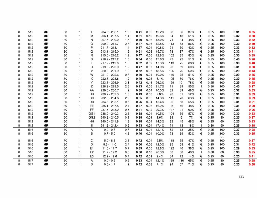
133
8 512 MR 80 1 L 204.8 - 206.1 1.3 0.41 0.05 12.2% 98 36 37% G 0.25 100 0.31 0.35 8 512 MR 80 1 M 206.1 - 207.5 1.4 0.51 0.10 19.6% 84 43 51% G 0.25 100 0.32 0.38 8 512 MR 80 1 N 207.5 - 209.0 1.5 0.40 0.06 15.0% 71 34 48% G 0.25 100 0.33 0.32 8 512 MR 80 1 O 209.0 - 211.7 2.7 0.47 0.06 12.8% 113 63 56% G 0.25 100 0.30 0.39 8 512 MR 80 1 P 211.7 - 213.1 1.4 0.37 0.04 10.8% 71 30 42% G 0.25 100 0.33 0.32 8 512 MR 80 1 Q 213.1 - 215.0 1.9 0.51 0.08 15.7% 78 37 47% G 0.25 100 0.32 0.41 8 512 MR 80 1 R 215.0 - 216.2 1.2 0.47 0.06 12.8% 102 85 83% G 0.25 100 0.30 0.39 8 512 MR 80 1 S 216.2 - 217.2 1.0 0.34 0.06 17.6% 43 22 51% G 0.25 100 0.40 0.26 8 512 MR 80 1 T 217.2 - 219.0 1.8 0.52 0.09 17.3% 113 75 66% G 0.25 100 0.30 0.40 8 512 MR 80 1 U 219.0 - 220.9 1.9 0.47 0.07 14.9% 98 59 60% G 0.25 100 0.31 0.38 8 512 MR 80 1 V 220.9 - 221.9 1.0 0.52 0.07 13.5% 126 76 60% G 0.25 100 0.29 0.43 8 512 MR 80 1 W 221.9 - 222.6 0.7 0.40 0.04 10.0% 146 75 51% G 0.25 100 0.29 0.35 8 512 MR 80 1 X 222.6 - 223.8 1.2 0.49 0.03 6.1% 105 80 76% G 0.25 100 0.30 0.45 8 512 MR 80 1 Y 223.8 - 226.9 3.1 0.42 0.11 26.2% 129 101 78% G 0.25 100 0.29 0.28 8 512 MR 80 1 Z 226.9 - 229.5 2.6 0.23 0.05 21.7% 71 39 55% I 0.30 100 0.40 0.17 8 512 MR 80 1 AA 229.5 - 230.7 1.2 0.38 0.04 10.5% 82 39 48% G 0.25 100 0.32 0.33 8 512 MR 80 1 BB 230.7 - 232.3 1.6 0.43 0.03 7.0% 98 51 52% G 0.25 100 0.31 0.39 8 512 MR 80 1 CC 232.3 - 234.6 2.3 0.35 0.05 14.3% 111 70 63% G 0.25 100 0.30 0.29 8 512 MR 80 1 DD 234.6 - 235.1 0.5 0.26 0.04 15.4% 96 53 55% G 0.25 100 0.31 0.21 8 512 MR 80 1 EE 235.1 - 237.5 2.4 0.37 0.06 16.2% 95 46 48% G 0.25 100 0.31 0.29 8 512 MR 80 1 FF 237.5 - 238.0 0.5 0.41 0.12 29.3% 147 91 62% G 0.25 100 0.29 0.26 8 512 MR 80 1 GG1 238.0 - 240.3 2.3 0.38 0.04 10.5% 104 59 57% G 0.25 100 0.30 0.33 8 512 MR 60 1 GG2 240.3 - 240.5 0.2 0.38 0.01 2.6% 89 6 7% G 0.25 80 0.25 0.37 8 512 MR 60 1 HH 240.5 - 241.8 1.3 0.28 0.04 14.3% 93 45 48% G 0.25 60 0.25 0.23 8 512 MR 50 1 II 241.8 - 242.4 0.6 0.23 0.04 17.4% 71 13 18% I 0.30 50 0.26 0.18 8 516 MR 80 1 A 0.0 - 0.7 0.7 0.33 0.04 12.1% 52 13 25% G 0.25 100 0.37 0.28 8 516 MR 80 1 B 0.7 - 5.0 4.3 0.40 0.04 10.0% 73 39 53% G 0.25 100 0.33 0.35
8 516 MR 70 1 C 5.0 - 8.6 3.6 0.42 0.04 9.5% 118 55 47% G 0.25 80-100 0.27 0.37
8 516 MR 80 1 D 8.6 - 11.0 2.4 0.50 0.06 12.0% 95 58 61% G 0.25 100 0.31 0.42 8 516 MR 80 1 E1 11.0 - 11.7 0.7 0.39 0.05 12.8% 122 46 38% G 0.25 100 0.29 0.33 8 516 MR 60 1 E2 11.7 - 12.2 0.5 0.38 0.10 26.3% 80 38 48% I 0.30 60 0.30 0.25 8 516 MR 60 1 E3 12.2 - 12.6 0.4 0.42 0.01 2.4% 84 12 14% G 0.25 80 0.25 0.41 8 517 MR 60 1 A 0.0 - 0.5 0.5 0.33 0.04 12.1% 169 110 65% G 0.25 80 0.25 0.28 8 517 MR 60 1 B 0.5 - 1.7 1.2 0.42 0.03 7.1% 94 67 71% G 0.25 80 0.25 0.38

134
8 517 MR 60 1 C 1.7 - 2.3 0.6 0.38 0.04 10.5% 81 49 60% G 0.25 80 0.25 0.33 8 517 MR 80 1 D 2.3 - 5.9 3.6 0.44 0.06 13.6% 129 73 57% G 0.25 100 0.29 0.36 8 517 MR 80 1 E 5.9 - 7.1 1.2 0.38 0.07 18.4% 88 30 34% G 0.25 100 0.31 0.29 8 517 MR 80 1 F 7.1 - 10.5 3.4 0.51 0.07 13.7% 143 67 47% G 0.25 100 0.29 0.42 8 517 MR 80 1 G 10.5 - 17.5 7.0 0.43 0.07 16.3% 109 78 72% G 0.25 100 0.30 0.34 8 517 MR 80 1 H 17.5 - 18.0 0.5 0.50 0.08 16.0% 90 93 103% G 0.25 100 0.31 0.40 8 517 MR 80 1 I 18.0 - 21.8 3.8 0.47 0.08 17.0% 106 73 69% G 0.25 100 0.30 0.37 8 517 MR 80 1 J 21.8 - 25.5 3.7 0.43 0.06 14.0% 114 86 75% G 0.25 100 0.30 0.35 8 517 MR 60 1 K 25.5 - 26.3 0.8 0.42 0.08 19.0% 86 70 81% G 0.25 80 0.25 0.32 8 518 MR 60 1 A 0.0 - 0.3 0.3 0.28 0.03 10.7% 66 10 15% G 0.25 80 0.25 0.24 8 518 MR 80 1 B 0.3 - 1.6 1.3 0.37 0.02 5.4% 127 57 45% G 0.25 100 0.29 0.34 8 518 MR 80 1 C 1.6 - 3.2 1.6 0.46 0.04 8.7% 101 60 59% G 0.25 100 0.30 0.41 8 518 MR 80 1 D 3.2 - 5.2 2.0 0.52 0.03 5.8% 113 56 50% G 0.25 100 0.30 0.48 8 518 MR 80 1 E 5.2 - 5.8 0.6 0.46 0.03 6.5% 96 61 64% G 0.25 100 0.31 0.42 8 518 MR 80 1 F 5.8 - 10.4 4.6 0.36 0.06 16.7% 92 63 68% G 0.25 100 0.31 0.28 8 530 MR 60 1 A 0.0 - 1.0 1.0 0.33 0.01 3.0% 90 21 23% G 0.25 60 0.25 0.32 8 530 MR 60 1 B1 1.0 - 1.8 0.8 0.28 0.08 28.6% 128 90 70% I 0.30 60 0.30 0.18 8 530 MR 40 1 B2 1.8 - 2.2 0.4 0.30 0.04 13.3% 93 44 47% I 0.30 40 0.24 0.25 8 530 MR 60 1 B3 2.2 - 2.5 0.3 0.29 0.05 17.2% 118 99 84% G 0.30 40 0.30 0.23 8 530 MR 60 1 C 2.5 - 3.0 0.5 0.27 0.02 7.4% 73 27 37% G 0.25 60 0.25 0.24 8 530 MR 60 1 D 3.0 - 3.8 0.8 0.37 0.04 10.8% 37 11 30% G 0.25 80 0.25 0.32 8 530 MR 60 1 E 3.8 - 4.3 0.5 0.31 0.02 6.5% 59 34 58% G 0.25 60 0.25 0.28 8 531 MR 60 1 A 0.0 - 0.4 0.4 0.30 0.03 10.0% 67 20 30% I 0.30 70 0.30 0.26 8 531 MR 60 1 B 0.4 - 1.9 1.5 0.33 0.02 6.1% 85 15 18% I 0.30 70 0.30 0.30 8 531 MR 60 1 C 1.9 - 3.5 1.6 0.22 0.05 22.7% 65 52 80% I 0.30 60 0.30 0.16 8 532 MR 80 1 A 0.0 - 0.5 0.5 0.26 0.03 11.5% 95 33 35% G 0.25 100 0.31 0.22 8 532 MR 80 1 B 0.5 - 3.2 2.7 0.35 0.03 8.6% 121 70 58% G 0.25 100 0.29 0.31 8 532 MR 60 1 C1 3.2 - 4.1 0.9 0.42 0.02 4.8% 105 39 37% G 0.25 80 0.25 0.39 8 532 MR 70 1 C2 4.1 - 5.6 1.5 0.45 0.03 6.7% 105 42 40% G 0.25 90 0.27 0.41 8 532 MR 60 1 D1 5.6 - 6.3 0.7 0.37 0.02 5.4% 110 42 38% I 0.30 70 0.30 0.34 8 532 MR 80 1 D2 6.3 - 9.5 3.2 0.37 0.05 13.5% 111 53 48% G 0.25 100 0.30 0.31 8 532 MR 80 1 E1 9.5 - 14.8 5.3 0.35 0.03 8.6% 107 57 53% G 0.25 100 0.30 0.31 8 532 MR 60 1 E2 14.8 - 16.0 1.2 0.35 0.03 8.6% 84 30 36% I 0.30 60 0.30 0.31 8 532 MR 60 1 F 16.0 - 18.1 2.1 0.26 0.04 15.4% 88 30 34% I 0.30 60 0.30 0.21 8 532 MR 80 1 G 18.1 - 20.2 2.1 0.37 0.02 5.4% 140 71 51% G 0.25 100 0.29 0.34
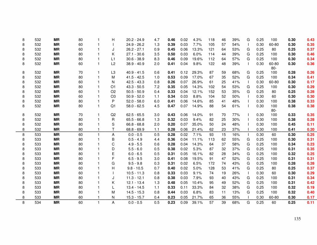
135
8 532 MR 80 1 H 20.2 - 24.9 4.7 0.46 0.02 4.3% 118 46 39% G 0.25 100 0.30 0.43 8 532 MR 60 1 I 24.9 - 26.2 1.3 0.39 0.03 7.7% 105 57 54% I 0.30 60-80 0.30 0.35 8 532 MR 60 1 J 26.2 - 27.1 0.9 0.45 0.06 13.3% 121 64 53% G 0.25 80 0.25 0.37 8 532 MR 80 1 K 27.1 - 30.6 3.5 0.50 0.03 6.0% 114 44 39% G 0.25 100 0.30 0.46 8 532 MR 80 1 L1 30.6 - 38.9 8.3 0.46 0.09 19.6% 112 64 57% G 0.25 100 0.30 0.34 8 532 MR 60 1 L2 38.9 - 40.9 2.0 0.41 0.04 9.8% 122 48 39% I 0.30 60-80 0.30 0.36
8 532 MR 70 1 L3 40.9 - 41.5 0.6 0.41 0.12 29.3% 87 59 68% G 0.25 80-100 0.28 0.26
8 532 MR 80 1 M 41.5 - 42.5 1.0 0.53 0.09 17.0% 67 35 52% G 0.25 100 0.34 0.41 8 532 MR 60 1 N 42.5 - 43.3 0.8 0.26 0.07 26.9% 61 25 41% I 0.30 60-80 0.30 0.17 8 532 MR 80 1 O1 43.3 - 50.5 7.2 0.35 0.05 14.3% 102 54 53% G 0.25 100 0.30 0.29 8 532 MR 60 1 O2 50.5 - 50.9 0.4 0.33 0.04 12.1% 152 53 35% G 0.25 80 0.25 0.28 8 532 MR 60 1 O3 50.9 - 52.0 1.1 0.34 0.03 8.8% 104 52 50% I 0.30 60 0.30 0.30 8 532 MR 80 1 P 52.0 - 58.0 6.0 0.41 0.06 14.6% 85 41 48% I 0.30 100 0.38 0.33 8 532 MR 80 1 Q1 58.0 - 62.5 4.5 0.47 0.07 14.9% 88 54 61% I 0.30 100 0.38 0.38
8 532 MR 70 1 Q2 62.5 - 65.5 3.0 0.43 0.06 14.0% 91 70 77% I 0.30 80-100 0.33 0.35
8 532 MR 80 1 R 65.5 - 66.8 1.3 0.32 0.03 9.4% 82 25 30% I 0.30 100 0.38 0.28 8 532 MR 80 1 S 66.8 - 68.8 2.0 0.20 0.07 35.0% 50 24 48% I 0.30 100 0.45 0.11 8 532 MR 80 1 T 68.8 - 69.9 1.1 0.28 0.06 21.4% 62 23 37% I 0.30 100 0.41 0.20 8 533 MR 60 1 A 0.0 - 0.5 0.5 0.28 0.02 7.1% 93 15 16% I 0.30 60 0.30 0.25 8 533 MR 80 1 B 0.5 - 4.9 4.4 0.36 0.04 11.1% 113 62 55% G 0.25 100 0.30 0.31 8 533 MR 80 1 C 4.9 - 5.5 0.6 0.28 0.04 14.3% 64 37 58% G 0.25 100 0.34 0.23 8 533 MR 80 1 D 5.5 - 6.0 0.5 0.38 0.02 5.3% 87 32 37% G 0.25 100 0.31 0.35 8 533 MR 80 1 E 6.0 - 6.5 0.5 0.31 0.05 16.1% 82 28 34% G 0.25 100 0.32 0.25 8 533 MR 80 1 F 6.5 - 9.5 3.0 0.41 0.08 19.5% 91 47 52% G 0.25 100 0.31 0.31 8 533 MR 80 1 G 9.5 - 9.8 0.3 0.31 0.02 6.5% 172 74 43% G 0.25 100 0.28 0.28 8 533 MR 60 1 H 9.8 - 10.5 0.7 0.40 0.02 5.0% 128 53 41% G 0.25 80 0.25 0.37 8 533 MR 60 1 I 10.5 - 11.3 0.8 0.33 0.03 9.1% 74 19 26% I 0.30 60 0.30 0.29 8 533 MR 80 1 J 11.3 - 12.1 0.8 0.38 0.03 7.9% 93 40 43% G 0.25 100 0.31 0.34 8 533 MR 80 1 K 12.1 - 13.4 1.3 0.48 0.05 10.4% 95 49 52% G 0.25 100 0.31 0.42 8 533 MR 80 1 L 13.4 - 14.5 1.1 0.33 0.11 33.3% 84 32 38% G 0.25 100 0.32 0.19 8 533 MR 80 1 M 14.5 - 15.3 0.8 0.44 0.03 6.8% 83 11 13% G 0.25 100 0.32 0.40 8 533 MR 60 1 N 15.3 - 15.7 0.4 0.23 0.05 21.7% 65 36 55% I 0.30 60-80 0.30 0.17 8 534 MR 60 1 A 0.0 - 0.5 0.5 0.23 0.09 39.1% 57 39 68% G 0.25 60 0.25 0.11

136
8 534 MR 80 1 B 0.5 - 4.3 3.8 0.44 0.05 11.4% 105 49 47% G 0.25 100 0.30 0.38 8 534 MR 80 1 C 4.3 - 4.9 0.6 0.32 0.04 12.5% 53 28 53% G 0.25 100 0.36 0.27 8 534 MR 80 1 D 4.9 - 6.4 1.5 0.42 0.03 7.1% 92 69 75% G 0.25 100 0.31 0.38 8 534 MR 80 1 E 6.4 - 8.6 2.2 0.46 0.05 10.9% 117 51 44% G 0.25 100 0.30 0.40 8 534 MR 1 F 8.6 - 12.2 8 534 MR 80 1 G 12.2 - 12.7 0.5 0.43 0.03 7.0% 85 31 36% G 0.25 100 0.32 0.39 8 534 MR 80 1 H 12.7 - 16.8 4.1 0.54 0.08 14.8% 96 46 48% G 0.25 100 0.31 0.44 8 534 MR 80 1 I 16.8 - 17.1 0.3 0.30 0.02 6.7% 81 39 48% G 0.25 100 0.32 0.27 8 534 MR 80 1 J 17.1 - 18.4 1.3 0.45 0.05 11.1% 90 51 57% G 0.25 100 0.31 0.39 8 534 MR 80 1 K 18.4 - 18.7 0.3 0.20 0.03 15.0% 55 13 24% G 0.25 100 0.36 0.16 8 534 MR 80 1 L 18.7 - 23.0 4.3 0.40 0.06 15.0% 90 44 49% G 0.25 100 0.31 0.32 8 535 MR 60 1 A 0.0 - 0.5 0.5 0.29 0.06 20.7% 94 38 40% G 0.25 60 0.25 0.21
8 535 MR 70 1 B 0.5 - 1.6 1.1 0.38 0.03 7.9% 116 39 34% G 0.25 80-100 0.27 0.34
8 535 MR 80 1 C 1.6 - 3.5 1.9 0.43 0.02 4.7% 137 65 47% G 0.25 100 0.29 0.40
8 535 MR 70 1 D 3.5 - 5.0 1.5 0.46 0.03 6.5% 122 62 51% G 0.25 80-100 0.27 0.42
8 535 MR 60 1 E 5.0 - 5.5 0.5 0.36 0.03 8.3% 81 13 16% G 0.25 80 0.25 0.32 8 535 MR 80 1 F 5.5 - 8.4 2.9 0.39 0.05 12.8% 91 70 77% G 0.25 100 0.31 0.33 8 535 MR 80 1 G 8.4 - 8.8 0.4 0.30 0.03 10.0% 75 51 68% G 0.25 100 0.33 0.26 8 536 MR 60 1 A 0.0 - 0.2 0.2 0.27 0.01 3.7% 122 58 48% G 0.25 80 0.25 0.26 8 536 MR 80 1 B 0.2 - 0.8 0.6 0.28 0.02 7.1% 100 56 56% G 0.25 100 0.31 0.25 8 536 MR 80 1 C 0.8 - 1.2 0.4 0.37 0.02 5.4% 45 5 11% G 0.25 100 0.39 0.34 8 536 MR 80 1 D 1.2 - 1.8 0.6 0.27 0.06 22.2% 42 23 55% G 0.25 100 0.40 0.19 8 536 MR 80 1 E 1.8 - 3.8 2.0 0.39 0.06 15.4% 63 39 62% G 0.25 100 0.34 0.31 8 536 MR 80 1 F 3.8 - 6.8 3.0 0.36 0.08 22.2% 69 60 87% G 0.25 100 0.33 0.26 8 536 MR 80 1 G 6.8 - 7.9 1.1 0.37 0.03 8.1% 70 34 49% G 0.25 100 0.33 0.33 8 536 MR 80 1 H 7.9 - 9.5 1.6 0.47 0.06 12.8% 101 64 63% G 0.25 100 0.30 0.39 8 536 MR 80 1 I 9.5 - 15.2 5.7 0.40 0.04 10.0% 88 61 69% G 0.25 100 0.31 0.35 8 536 MR 80 1 J 15.2 - 20.8 5.6 0.35 0.06 17.1% 56 26 46% G 0.25 100 0.36 0.27 8 536 MR 80 1 K 20.8 - 23.1 2.3 0.40 0.06 15.0% 63 37 59% G 0.25 100 0.34 0.32 8 536 MR 80 1 L 23.1 - 23.5 0.4 0.28 0.09 32.1% 71 48 68% G 0.25 100 0.33 0.16 8 536 MR 80 1 M 23.5 - 28.6 5.1 0.48 0.04 8.3% 104 57 55% G 0.25 100 0.30 0.43 8 536 MR 80 1 N 28.6 - 32.5 3.9 0.44 0.12 27.3% 82 67 82% G 0.25 100 0.32 0.29 8 536 MR 80 1 O 32.8 - 38.3 5.5 0.35 0.09 25.7% 77 59 77% G 0.25 100 0.32 0.23

137
8 851 MR 60 1 A1 0.0 - 0.3 0.3 0.23 0.06 26.1% 148 137 93% G 0.25 60 0.25 0.15 8 851 MR 80 1 A2 0.3 - 1.7 1.4 0.30 0.03 10.0% 103 59 57% G 0.25 100 0.30 0.26 8 851 MR 80 1 B 1.7 - 5.4 3.7 0.38 0.02 5.3% 101 46 46% G 0.25 100 0.30 0.35 8 851 MR 80 1 C 5.4 - 12.6 7.2 0.37 0.03 8.1% 109 63 58% G 0.25 100 0.30 0.33 8 851 MR 80 1 D 12.6 - 17.2 4.6 0.34 0.03 8.8% 96 40 42% G 0.25 100 0.31 0.30 8 851 MR 70 1 E1 17.2 - 17.5 0.3 0.32 0.01 3.1% 71 8 11% G 0.25 90 0.29 0.31 8 851 MR 60 1 E2 17.5 - 19.3 1.8 0.29 0.04 13.8% 72 21 29% I 0.30 70 0.30 0.24 8 851 MR 60 1 F 19.3 - 22.8 3.5 0.31 0.03 9.7% 70 26 37% I 0.30 60 0.30 0.27 8 851 MR 50 1 G 22.8 - 24.0 1.2 0.24 0.04 16.7% 61 18 30% I 0.30 50 0.25 0.19 8 851 MR 60 1 H 24.0 - 25.4 1.4 0.31 0.03 9.7% 93 27 29% G 0.25 70 0.25 0.27 8 851 MR 60 1 I 25.4 - 26.6 1.2 0.36 0.03 8.3% 114 59 52% G 0.25 80 0.25 0.32 8 851 MR 80 1 J1 26.6 - 28.3 1.7 0.36 0.03 8.3% 62 31 50% G 0.25 100 0.35 0.32 8 851 MR 80 1 J2 28.3 - 30.6 2.3 0.40 0.03 7.5% 90 46 51% G 0.25 100 0.31 0.36 8 851 MR 60 1 K 30.6 - 31.2 0.6 0.32 0.10 31.3% 93 48 52% G 0.25 80 0.25 0.19 8 851 MR 60 1 L 31.2 - 33.7 2.5 0.30 0.07 23.3% 67 40 60% G 0.25 60 0.25 0.21 8 852 MR 60 1 A1 0.0 - 0.5 0.5 0.50 0.05 10.0% 80 10 13% G 0.25 60 0.25 0.44 8 852 MR 60 1 A2 0.5 - 1.8 1.3 0.43 0.03 7.0% 110 38 35% G 0.25 60 0.25 0.39 8 852 MR 80 1 B 1.8 - 2.2 0.4 0.31 0.02 6.5% 90 23 26% G 0.25 100 0.31 0.28 8 852 MR 80 1 C 2.2 - 3.5 1.3 0.38 0.02 5.3% 104 43 41% G 0.25 100 0.30 0.35 8 852 MR 80 1 D 3.5 - 8.3 4.8 0.44 0.05 11.4% 89 36 40% G 0.25 100 0.31 0.38
8 852 MR 70 1 E 8.3 - 11.6 3.3 0.55 0.03 5.5% 123 40 33% G 0.25 80-100 0.27 0.51
8 852 MR 60 1 F 11.6 - 14.1 2.5 0.51 0.06 11.8% 111 50 45% G 0.25 60 0.25 0.43 8 854 MR 80 1 A 0.0 - 0.7 0.7 0.33 0.05 15.2% 61 39 64% G 0.25 100 0.35 0.27 8 854 MR 80 1 B 0.7 - 1.6 0.9 0.44 0.04 9.1% 113 45 40% G 0.25 100 0.30 0.39 8 854 MR 80 1 C 1.6 - 1.8 0.2 0.27 0.02 7.4% 42 10 24% G 0.25 100 0.40 0.24 8 854 MR 80 1 D 1.8 - 5.1 3.3 0.42 0.04 9.5% 115 84 73% G 0.25 100 0.30 0.37 8 854 MR 80 1 E 5.1 - 7.7 2.6 0.50 0.04 8.0% 102 60 59% G 0.25 100 0.30 0.45 8 855 MR 60 1 A 0.0 - 0.7 0.7 0.37 0.04 10.8% 76 23 30% I 0.30 70 0.30 0.32 8 855 MR 80 1 B 0.7 - 3.3 2.6 0.44 0.06 13.6% 90 47 52% I 0.30 100 0.37 0.36 8 855 MR 80 1 C 3.3 - 4.6 1.3 0.38 0.06 15.8% 92 75 82% G 0.25 100 0.31 0.30 8 855 MR 80 1 D 4.6 - 7.0 2.4 0.51 0.06 11.8% 93 32 34% G 0.25 100 0.31 0.43 8 855 MR 80 1 E 7.0 - 8.5 1.5 0.35 0.07 20.0% 69 41 59% G 0.25 100 0.33 0.26 8 855 MR 80 1 F 8.5 - 9.2 0.7 0.48 0.05 10.4% 97 27 28% G 0.25 100 0.31 0.42 8 855 MR 80 1 G 9.2 - 11.8 2.6 0.38 0.08 21.1% 110 82 75% G 0.25 100 0.30 0.28

138
8 855 MR 80 1 H 11.8 - 12.9 1.1 0.32 0.03 9.4% 112 47 42% G 0.25 100 0.30 0.28 8 855 MR 80 1 I 12.9 - 13.7 0.8 0.40 0.07 17.5% 115 104 90% G 0.25 100 0.30 0.31 8 855 MR 80 1 J 13.7 - 20.4 6.7 0.42 0.07 16.7% 101 75 74% G 0.25 100 0.30 0.33 8 855 MR 70 1 K1 20.4 - 22.5 2.1 0.38 0.05 13.2% 91 60 66% G 0.25 100 0.28 0.32 8 855 MR 60 1 K2 22.5 - 23.1 0.6 0.38 0.02 5.3% 89 34 38% I 0.30 60-80 0.30 0.35 8 855 MR 60 1 L 23.1 - 23.4 0.3 0.23 0.04 17.4% 46 7 15% I 0.30 60 0.30 0.18 8 856 MR 60 1 A 0.0 - 0.7 0.7 0.25 0.07 28.0% 64 20 31% I 0.30 60 0.30 0.16 8 856 MR 60 1 B1 0.7 - 1.5 0.8 0.35 0.02 5.7% 100 38 38% G 0.25 60 0.25 0.32 8 856 MR 60 1 B2 1.5 - 2.7 1.2 0.34 0.04 11.8% 85 27 32% G 0.25 80 0.25 0.29 8 856 MR 60 1 C 2.7 - 4.3 1.6 0.39 0.03 7.7% 84 33 39% G 0.25 80 0.25 0.35 8 856 MR 60 1 D 4.3 - 7.6 3.3 0.32 0.05 15.6% 94 43 46% I 0.30 60 0.30 0.26 8 856 MR 70 1 E1 7.6 - 9.0 1.4 0.40 0.02 5.0% 117 27 23% G 0.25 90 0.27 0.37 8 856 MR 60 1 E2 9.0 - 10.2 1.2 0.37 0.02 5.4% 105 37 35% G 0.25 80 0.25 0.34 8 856 MR 60 1 E3 10.2 - 10.8 0.6 0.38 0.04 10.5% 83 23 28% G 0.25 60 0.25 0.33 8 857 MR 60 1 A 0.0 - 0.4 0.4 0.31 0.01 3.2% 125 49 39% I 0.30 60 0.30 0.30 8 857 MR 60 1 B 0.4 - 0.7 0.3 0.22 0.02 9.1% 55 17 31% I 0.30 60 0.30 0.19 8 857 MR 60 1 C 0.7 - 0.9 0.2 0.30 0.01 3.3% 92 8 9% I 0.30 60 0.30 0.29 8 857 MR 60 1 D 0.9 - 1.9 1.0 0.22 0.03 13.6% 61 12 20% I 0.30 60 0.30 0.18 8 857 MR 60 1 E 1.9 - 3.0 1.1 0.30 0.02 6.7% 83 20 24% I 0.30 60 0.30 0.27 8 857 MR 60 1 F 3.0 - 3.3 0.3 0.21 0.04 19.0% 52 19 37% I 0.30 60 0.30 0.16 8 857 MR 60 1 G 3.3 - 4.3 1.0 0.31 0.02 6.5% 89 19 21% G 0.25 80 0.25 0.28 8 857 MR 60 1 H 4.3 - 5.7 1.4 0.40 0.03 7.5% 92 20 22% G 0.25 80 0.25 0.36 8 857 MR 60 1 I 5.7 - 6.2 0.5 0.32 0.03 9.4% 106 46 43% G 0.25 80 0.25 0.28 8 857 MR 80 1 J 6.2 - 7.4 1.2 0.43 0.05 11.6% 98 35 36% G 0.25 100 0.31 0.37 8 857 MR 60 1 K 7.4 - 7.8 0.4 0.43 0.01 2.3% 145 52 36% G 0.25 80 0.25 0.42 8 857 MR 60 1 L 7.8 - 8.5 0.7 0.36 0.02 5.6% 122 39 32% I 0.30 60 0.30 0.33 8 857 MR 60 1 M 8.5 - 9.6 1.1 0.40 0.04 10.0% 91 51 56% I 0.30 60 0.30 0.35 8 857 MR 60 1 N 9.6 - 10.3 0.7 0.28 0.07 25.0% 69 31 45% I 0.30 60 0.30 0.19 8 857 MR 60 1 O 10.3 - 11.0 0.7 0.37 0.04 10.8% 115 75 65% I 0.30 60 0.30 0.32 8 857 MR 60 1 P 11.0 - 12.1 1.1 0.42 0.04 9.5% 101 57 56% I 0.30 60 0.30 0.37 8 5126 SR 60 1 A 0.0 - 0.4 0.4 0.32 0.04 12.5% 105 55 52% I 0.30 60-80 0.30 0.27 8 5126 SR 80 1 B 0.4 - 0.7 0.3 0.26 0.02 7.7% 98 21 21% G 0.25 100 0.31 0.23 8 5126 SR 80 1 C 0.7 - 2.0 1.3 0.41 0.05 12.2% 97 50 52% G 0.25 100 0.31 0.35 8 5126 SR 80 1 D 2.0 - 2.5 0.5 0.57 0.12 21.1% 97 50 52% G 0.25 100 0.31 0.42 8 5126 SR 80 1 E 2.5 - 3.5 1.0 0.48 0.07 14.6% 118 88 75% G 0.25 100 0.30 0.39

139
8 5302 SR 60 1 A1 0.0 - 0.4 0.4 0.33 0.03 9.1% 75 32 43% I 0.30 60 0.30 0.29 8 5302 SR 60 1 A2 0.4 - 1.3 0.9 0.34 0.03 8.8% 77 25 32% G 0.25 80 0.25 0.30 8 5302 SR 60 1 B 1.3 - 1.8 0.5 0.28 0.05 17.9% 75 40 53% G 0.25 60 0.25 0.22 8 5302 SR 80 1 C 1.8 - 2.9 1.1 0.40 0.05 12.5% 94 49 52% G 0.25 100 0.31 0.34 8 5302 SR 80 1 D 2.9 - 3.5 0.6 0.29 0.03 10.3% 72 27 38% G 0.25 100 0.33 0.25 8 5302 SR 80 1 E 3.5 - 9.1 5.6 0.48 0.06 12.5% 92 40 43% G 0.25 100 0.31 0.40 8 5302 SR 80 1 F 9.1 - 10.9 1.8 0.43 0.06 14.0% 68 39 57% G 0.25 100 0.34 0.35 8 5302 SR 80 1 G 10.9 - 13.2 2.3 0.50 0.10 20.0% 106 68 64% G 0.25 100 0.30 0.37 8 5302 SR 80 1 H 13.2 - 13.6 0.4 0.33 0.07 21.2% 70 37 53% G 0.25 100 0.33 0.24 8 5302 SR 80 1 I 13.6 - 17.3 3.7 0.51 0.06 11.8% 107 59 55% G 0.25 100 0.30 0.43 8 5302 SR 80 1 J 17.3 - 18.1 0.8 0.46 0.06 13.0% 120 24 20% G 0.25 100 0.30 0.38 8 5302 SR 80 1 K 18.1 - 19.0 0.9 0.39 0.05 12.8% 69 27 39% G 0.25 100 0.33 0.33 8 5302 SR 80 1 L 19.0 - 22.0 3.0 0.46 0.08 17.4% 78 52 67% G 0.25 100 0.32 0.36 8 5302 SR 1 M 22.0 - 23.0 8 5302 SR 80 1 N 23.0 - 24.3 1.3 0.48 0.06 12.5% 102 90 88% G 0.25 100 0.30 0.40 8 5302 SR 60 1 O 24.3 - 24.1 0.1 0.28 0.02 7.1% 46 10 22% G 0.25 80 0.25 0.25 8 5323 SR 60 1 A1 0.0 - 0.4 0.4 0.24 0.05 20.8% 58 18 31% I 0.30 60 0.30 0.18 8 5323 SR 60 1 A2 0.4 - 0.8 0.4 0.35 0.04 11.4% 133 70 53% I 0.30 60 0.30 0.30 8 5323 SR 80 1 B 0.8 - 1.9 1.1 0.35 0.02 5.7% 83 34 41% G 0.25 100 0.32 0.32 8 5323 SR 80 1 C 1.9 - 3.0 1.1 0.44 0.04 9.1% 100 45 45% G 0.25 100 0.31 0.39 8 5323 SR 80 1 D 3.0 - 3.4 0.4 0.56 0.02 3.6% 89 43 48% G 0.25 100 0.31 0.53 8 5323 SR 80 1 E 3.4 - 5.6 2.2 0.52 0.05 9.6% 105 48 46% G 0.25 100 0.30 0.46 8 5323 SR 80 1 F 5.6 - 6.9 1.3 0.48 0.06 12.5% 99 49 49% G 0.25 100 0.31 0.40 8 5323 SR 80 1 G 6.9 - 8.8 1.9 0.38 0.06 15.8% 100 48 48% G 0.25 100 0.31 0.30 8 5323 SR 80 1 H 8.8 -- 11.3 2.5 0.48 0.05 10.4% 119 68 57% G 0.25 100 0.30 0.42 8 5323 SR 80 1 I 11.3 - 13.3 2.0 0.45 0.06 13.3% 89 67 75% G 0.25 100 0.31 0.37 8 5323 SR 1 J 13.3 - 14.2 8 5323 SR 80 1 K 14.2 - 14.4 0.2 0.43 0.01 2.3% 83 12 14% G 0.25 100 0.32 0.42 8 5323 SR 1 L 14.4 - 15.3 8 5323 SR 80 1 M 15.3 - 17.6 2.3 0.47 0.07 14.9% 107 37 35% G 0.25 100 0.30 0.38 8 5324 SR 60 1 A 0.0 - 0.9 0.9 0.40 0.06 15.0% 76 19 25% I 0.30 60 0.30 0.32 8 5324 SR 60 1 B 0.9 - 1.3 0.4 0.39 0.02 5.1% 70 20 29% I 0.30 80 0.30 0.36 8 5324 SR 80 1 C 1.3 - 3.0 1.7 0.44 0.04 9.1% 81 26 32% I 0.30 100 0.38 0.39 8 5324 SR 80 1 D 3.0 - 4.4 1.4 0.52 0.04 7.7% 98 39 40% I 0.30 100 0.37 0.47 8 5324 SR 80 1 E 4.4 - 5.0 0.6 0.46 0.03 6.5% 99 24 24% I 0.30 100 0.37 0.42

140
8 5324 SR 50 1 F 5.0 - 5.5 0.5 0.38 0.05 13.2% 64 34 53% I 0.30 50 0.26 0.32 8 5324 SR 60 1 G 5.5 - 6.0 0.5 0.44 0.05 11.4% 86 37 43% I 0.30 80 0.30 0.38 8 5324 SR 80 1 H 6.0 - 7.4 1.4 0.47 0.05 10.6% 101 28 28% I 0.30 100 0.37 0.41 8 5332 SR 60 1 A 0.0 - 0.6 0.6 0.33 0.06 18.2% 55 28 51% I 0.30 60 0.30 0.25 8 5332 SR 80 1 B 0.6 - 2.9 2.3 0.47 0.04 8.5% 108 55 51% G 0.25 100 0.30 0.42 8 5332 SR 80 1 C 2.9 - 3.8 0.9 0.36 0.05 13.9% 72 38 53% G 0.25 100 0.33 0.30 8 5342 SR 80 1 A 0.0 - 0.6 0.6 0.37 0.04 10.8% 58 16 28% G 0.25 100 0.35 0.32 8 5342 SR 80 1 B 0.6 - 4.8 4.2 0.44 0.05 11.4% 86 48 56% G 0.25 100 0.32 0.38 8 5342 SR 80 1 C 4.8 - 5.1 0.3 0.36 0.02 5.6% 69 18 26% G 0.25 100 0.33 0.33 8 5382 SR 60 1 A 0.0 - 0.3 0.3 0.24 0.02 8.3% 56 10 18% I 0.30 60 0.30 0.21 8 5382 SR 40 1 B1 0.3 - 1.0 0.7 0.18 0.03 16.7% 55 18 33% I 0.30 40 0.21 0.14 8 5382 SR 60 1 B2 1.0 - 2.5 1.5 0.23 0.04 17.4% 57 22 39% I 0.30 60 0.30 0.18 8 5382 SR 60 1 C 2.5 - 3.5 1.0 0.31 0.03 9.7% 82 50 61% G 0.25 80 0.25 0.27 8 5382 SR 80 1 D 3.5 - 5.5 2.0 0.42 0.03 7.1% 118 61 52% G 0.25 100 0.30 0.38 8 5382 SR 80 1 E 5.5 - 15.6 10.1 0.45 0.05 11.1% 92 48 52% G 0.25 100 0.31 0.39 8 5382 SR 80 1 F 15.6 - 17.7 2.1 0.41 0.06 14.6% 91 49 54% G 0.25 100 0.31 0.33 8 5382 SR 80 1 G1 17.7 - 23.3 5.6 0.54 0.05 9.3% 95 60 63% G 0.25 100 0.31 0.48 8 5382 SR 60 1 G2 23.3 - 24.1 0.8 0.50 0.05 10.0% 96 16 17% G 0.25 80 0.25 0.44 8 5382 SR 60 1 H 24.1 - 24.6 0.5 0.41 0.07 17.1% 69 43 62% G 0.25 80 0.25 0.32 8 8501 SR 80 1 A 0.0 - 0.2 0.2 0.29 0.02 6.9% 95 13 14% I 0.30 100 0.37 0.26 8 8501 SR 80 1 B 0.2 - 0.9 0.7 0.46 0.03 6.5% 106 60 57% G 0.25 100 0.30 0.42 8 8501 SR 80 1 C 0.9 - 6.3 5.4 0.49 0.05 10.2% 101 51 50% G 0.25 100 0.30 0.43 8 8501 SR 80 1 D 6.3 - 11.8 5.5 0.40 0.05 12.5% 97 48 49% G 0.25 100 0.31 0.34 8 8501 SR 80 1 E 11.8 - 12.3 0.5 0.34 0.03 8.8% 78 19 24% G 0.25 100 0.32 0.30 8 8501 SR 1 F 12.3 - 13.1 8 8501 SR 80 1 G 13.1 - 14.2 1.1 0.28 0.06 21.4% 90 44 49% G 0.25 100 0.31 0.20 8 8506 SR 80 1 A 0.0 - 3.4 3.4 0.39 0.04 10.3% 111 32 29% G 0.25 100 0.30 0.34 8 8506 SR 60 1 B 3.4 - 4.3 0.9 0.34 0.03 8.8% 92 30 33% G 0.25 60 0.25 0.30 8 8506 SR 60 1 C 4.3 - 4.6 0.3 0.36 0.03 8.3% 153 14 9% G 0.25 80 0.25 0.32 8 8506 SR 80 1 D 4.6 - 6.4 1.8 0.48 0.03 6.3% 112 49 44% G 0.25 100 0.30 0.44 8 8506 SR 80 1 E 6.4 - 7.1 0.7 0.30 0.03 10.0% 43 29 67% I 0.30 100 0.48 0.26 8 8506 SR 80 1 F 7.1 - 9.0 1.9 0.48 0.03 6.3% 101 27 27% G 0.25 100 0.30 0.44 8 8506 SR 80 1 G 9.0 - 10.0 1.0 0.40 0.03 7.5% 106 27 25% G 0.25 100 0.30 0.36 8 8509 SR 60 1 A 0.0 - 0.2 0.2 0.24 0.04 16.7% 51 2 4% G 0.25 60 0.25 0.19

141
8 8509 SR 60 1 B 0.2 - 1.9 1.7 0.37 0.05 13.5% 96 52 54% G 0.25 60 0.25 0.31 8 8509 SR 60 1 C 1.9 - 2.5 0.6 0.44 0.02 4.5% 101 59 58% G 0.25 80 0.25 0.41 8 8509 SR 80 1 D 2.5 - 3.5 1.0 0.37 0.06 16.2% 164 104 63% G 0.25 100 0.28 0.29 8 8509 SR 80 1 E 3.5 - 6.5 3.0 0.42 0.05 11.9% 121 60 50% G 0.25 100 0.29 0.36 8 8509 SR 80 1 F 6.5 - 7.2 0.7 0.53 0.08 15.1% 110 74 67% G 0.25 100 0.30 0.43 8 8509 SR 80 1 G 7.2 - 9.4 2.2 0.43 0.07 16.3% 128 64 50% G 0.25 100 0.29 0.34 8 8509 SR 80 1 H 9.4 - 11.8 2.2 0.51 0.08 15.7% 117 88 75% G 0.25 100 0.30 0.41 8 8509 SR 60 1 I 11.8 - 12.2 0.4 0.49 0.10 20.4% 107 67 63% G 0.25 80 0.25 0.36 8 8509 SR 60 1 J 12.2 - 12.7 0.5 0.48 0.08 16.7% 75 32 43% G 0.25 60 0.25 0.38 8 8509 SR 50 1 K 12.7 - 13.1 0.4 0.33 0.12 36.4% 64 36 56% I 0.30 50 0.26 0.18 8 8554 SR 1 A 0.0 - 0.2 8 8554 SR 80 1 B 0.2 - 0.7 0.5 0.46 0.07 15.2% 130 41 32% G 0.25 100 0.29 0.37 8 8554 SR 1 C 0.7 - 3.8 8 8554 SR 80 1 D 3.8 - 4.2 0.4 0.35 0.02 5.7% 44 13 30% G 0.25 100 0.39 0.32 8 8554 SR 80 1 E 4.2 - 6.3 2.1 0.51 0.05 9.8% 78 38 49% G 0.25 100 0.32 0.45 8 8554 SR 80 1 F 6.3 - 7.0 0.7 0.42 0.01 2.4% 45 26 58% G 0.25 100 0.39 0.41 8 8554 SR 80 1 G 7.0 - 8.7 1.7 0.47 0.03 6.4% 97 55 57% G 0.25 100 0.31 0.43 8 8554 SR 60 1 H 8.7 - 9.2 0.5 0.42 0.02 4.8% 101 71 70% G 0.25 80 0.25 0.39 8 8554 SR 60 1 I 9.2 - 9.8 0.6 0.40 0.02 5.0% 100 24 24% G 0.25 60 0.25 0.37 8 8554 SR 60 1 J 9.8 - 10.3 0.5 0.29 0.03 10.3% 131 61 47% I 0.30 60 0.30 0.25 8 8554 SR 60 1 K 10.3 - 10.7 0.4 0.42 0.03 7.1% 124 43 35% G 0.25 60 0.25 0.38 8 8554 SR 80 1 L 10.7 - 11.3 0.6 0.30 0.08 26.7% 74 49 66% G 0.25 100 0.33 0.20 8 8565 SR 60 1 A 0.0 - 0.5 0.5 0.45 0.07 15.6% 85 21 25% G 0.25 60 0.25 0.36 8 8565 SR 60 1 B 0.5 - 1.7 1.2 0.49 0.03 6.1% 142 44 31% G 0.25 80 0.25 0.45 8 8565 SR 60 1 C 1.7 - 2.3 0.6 0.39 0.01 2.6% 118 26 22% G 0.25 80 0.25 0.38 8 8565 SR 60 1 D 2.3 - 2.7 0.4 0.29 0.08 27.6% 83 29 35% I 0.30 80 0.30 0.19 8 8565 SR 60 1 E 2.7 - 3.0 0.3 0.43 0.01 2.3% 107 17 16% G 0.25 80 0.25 0.42 8 8565 SR 60 1 F 3.0 - 3.5 0.5 0.40 0.01 2.5% 125 55 44% G 0.25 60 0.25 0.39 8 8565 SR 60 1 G 3.5 - 3.9 0.4 0.33 0.03 9.1% 94 24 26% G 0.25 60 0.25 0.29 8 8565 SR 50 1 H 3.9 - 4.6 0.7 0.34 0.05 14.7% 84 39 46% I 0.30 50 0.27 0.28 Unsealed Roadworks

142
Appendix C - Metadata

143
DIGITAL CADASTRAL DATA BASE Dataset ANZLIC Identifier: ANZQL0053000003 Title : Digital Cadastral Data Base (DCDB) Custodian Custodian: Department of Natural Resources and Mines (NR&M) Jurisdiction : Queensland Description Abstract : The DCDB is the spatial representation of the property boundaries and the related property descriptions of Queensland. The DCDB provides the map base for systems dealing with land and land related information and provides data in order to generate hard copy map products. The DCDB is a fundamental reference layer for spatial information systems in Queensland. Search Words: LAND
LAND Cadastral BOUNDARY Administrative
Geographic Extent Name : gds_redcliffe_u.qif Geographic Extent polygon: Extent Window -27.20 153.11, -27.20 153.11, -27.23 153.11, -27.23 153.11, -27.20 153.11 Data Currency Beginning Date: June 1983 Ending Date: Current Data Status Progress: Complete Maintenance and Update Frequency: Daily Access Stored Data Format: The DCDB is stored in a relational data base format managed by an INGRES RDBMS Version II 2.0/0001 on a SUN E880 server using a SunOS 5.8 operating system. The DCDB data is accessed using a three tier client / server application for viewing or the extraction of QIF data or the production of hardcopy mapping. Available Format Types:
• DIGITAL - QIF Grid / Geographic co-ordinate values - ASCII • DIGITAL - ArcInfo / ArcView • DIGITAL - Autocad DXF / DWG • DIGITAL - MicroStation DGN • DIGITAL - MapInfo • NON DIGITAL - Plotted maps • NON DIGITAL - Printouts • NON DIGITAL - Reports
The digital DCDB data is extracted in an interchange format, QIF (Queensland Interchange Format). This specification provides the digital data in a flat ASCII file format suitable for translation to proprietary systems. The specification is available as an NR&M QA document PBD/801/206 ver. 3.2. The QIF data can be provided in either datum, AGD84 or GDA94. The data is available in any of the standard co-ordinate systems below:-
• grid co-ordinates ( Eastings and Northings ) in metres using the Australian Map Grid 1984 (AGD84) co-ordinate set;
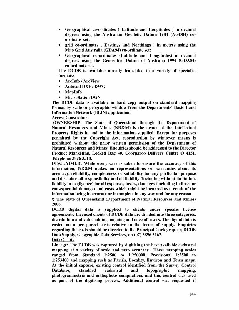
144
• Geographical co-ordinates ( Latitude and Longitudes ) in decimal degrees using the Australian Geodetic Datum 1984 (AGD84) co-ordinate set;
• grid co-ordinates ( Eastings and Northings ) in metres using the Map Grid Australia (GDA94) co-ordinate set;
• Geographical co-ordinates (Latitude and Longitudes) in decimal degrees using the Geocentric Datum of Australia 1994 (GDA84) co-ordinate set.
The DCDB is available already translated in a variety of specialist formats: • ArcInfo / ArcView • Autocad DXF / DWG • MapInfo • MicroStation DGN
The DCDB data is available in hard copy output on standard mapping format by scale or geographic window from the Departments' Basic Land Information Network (BLIN) application. Access Constraints: OWNERSHIP: The State of Queensland through the Department of Natural Resources and Mines (NR&M) is the owner of the Intellectual Property Rights in and to the information supplied. Except for purposes permitted by the Copyright Act, reproduction by whatever means is prohibited without the prior written permission of the Department of Natural Resources and Mines. Enquiries should be addressed to the Director Product Marketing, Locked Bag 40, Coorparoo Delivery Centre Q 4151. Telephone 3896 3518. DISCLAIMER: While every care is taken to ensure the accuracy of this information, NR&M makes no representations or warranties about its accuracy, reliability, completeness or suitability for any particular purpose and disclaims all responsibility and all liability (including without limitation, liability in negligence) for all expenses, losses, damages (including indirect or consequential damage) and costs which might be incurred as a result of the information being inaccurate or incomplete in any way and for any reason. The State of Queensland (Department of Natural Resources and Mines) 2005. DCDB digital data is supplied to clients under specific licence agreements. Licensed clients of DCDB data are divided into three categories, distribution and value adding, ongoing and once off users. The digital data is costed on a per parcel basis relative to the terms of supply. Enquiries regarding the costs should be directed to the Principal Cartographer, DCDB Data Supply, Geographic Data Services, on (07) 3896 3162. Data Quality Lineage: The DCDB was captured by digitising the best available cadastral mapping at a variety of scale and map accuracy. These mapping scales ranged from Standard 1:2500 to 1:250000, Provisional 1:2500 to 1:253400 and mapping such as Parish, Locality, Environ and Town maps. At the initial capture, existing control identified from the Survey Control Database, standard cadastral and topographic mapping, photogrammetric and orthophoto compilations and this control was used as part of the digitising process. Additional control was requested if

145
necessary. The DCDB is continuously updated by inputting metes and bounds descriptions from registered plans of subdivision and from any attribute updates from government gazettes and other administrative notifications. Selected areas of the DCDB are being upgraded for an improved positional accuracy, this is an ongoing process affected on a data or cost sharing basis with the user. The geodetic datum for the DCDB is GDA94. In October 2000, the datum of DCDB was converted from AGD84 values. A distortion model based on a Queensland grid was used in the transformation process for the conversion of the DCDB co-ordinate values from AGD84 to GDA94. Positional Accuracy: Positional accuracy values have been allocated all parcels in the DCDB. This value reflects 'maximum error' status of the parcel and has been derived from the capture process or assigned as the DCDB data has been upgraded. For this QIF extraction, the 'maximum error' of parcels range from: 0.10m to 0.10m. The data is sourced from: B&D plot controlled It has been established that the positional accuracy of the DCDB should include a finite value representing the 'maximum error' based on the source map type, the scale and a digitising value component. The calculated values linked to the source map scale is the root mean square error results of the precision of digitising and source map accuracy. Accuracy value have been applied to upgraded parcels, these values were determined at the time of upgrade and are dependent on the upgrade process. The values are expressed in metres at a 95% confidence level. Attribute Accuracy: The attributes in the DCDB are acquired from a number of sources within the Department. The attributes describe a range of characteristics about each land parcel such as property description, area, tenure, linestyle etc. Each polygon in the DCDB has a unique identifier called a segment-parcel number. The following attributes are attached to each polygon in the DCDB based on the polygon centroid which is the segment-parcel number Accuracy code Centroid value Coverage code Excluded area value Feature name Linestyle code Local Government code Locality code Locality name Lot area value Lot number Maximum error value Parcel indicator code Parcel type code Parcel number Parcel corner value Parcel count value Parish code Plan number Segment number Surveyed indicator Tenure code Update number Update type code Most attributes were validated after the initial capture of the DCDB and are updated as part of the maintenance process. The validation process consisted of the visual inspection/comparison of hard copy output compared to the departmental cadastral working maps and update plans. There are several system validation procedures in the maintenance process and these are run at a required frequency. The QIF data routine also provides a validation report on a data extract. The attributes of Locality and Parish have not been fully validated. A program for the capture of Locality data is in progress. As this locality data becomes available it will be reflected in the

146
database. As other departmental datasets of lot/plan data, (ie ATS, QVAS, CISP, TAS etc), become available they are matched to each other to improve the reliability of the Departments' databases. The estimated accuracy of the attribute information is 98%, this is exclusive of locality and parish information. Logical consistency: The current DCDB can be considered as a seamless map of the State and consists of base cadastral parcels, strata level parcels (secondary interests), volumetric and easement parcels. Base parcels are contiguous with surrounding base parcels. The graphic package and the routines that extract and reload update data to the database has a tolerance of 2mm on the ground. This tolerance may become significant in some proprietary systems and therefore an allowance will be necessary. Completeness: The DCDB data has been investigated for completeness by visual inspection of validation plots compared to the cadastral working maps and update plans. The update process for new graphics subdivisional data entered into the DCDB includes an extraction of a hard copy output after the update data is loaded back to the database for the data validation. When digital data is extracted from the DCDB in QIF, the extract routine provides a report on the completeness of the data extracted. If the data indicated errors then subsequent corrective action is taken before the data is re-extracted. Easements are being input as new plans of subdivision are updated in the database. The historical easements are being captured as a project. This capture over the whole of the State is not yet complete. Volumetric plans are being input as new plans of subdivision are updated in the database. Contact Information Contact Organisation: Department of Natural Resources and Mines, Queensland Contact Position: Manager, Geographic Data Services Mail Address: Locked Bag 40
Coorparoo Delivery Centre Qld 4151 Locality: Woolloongabba State: Queensland Country: Australia Post Code: 4102 Telephone: (07) 3896 3110 Facsimile: (07) 3896 3165 Email Address: [email protected] Metadata Date Metadata Date: 15/05/2005 Additional Metadata Additional Metadata: Further information about the supply of the DCDB in specific digital formats is available from the Principal Cartographer, DCDB Data Supply, Geographic Data Services, on (07) 3896 3162 or Email [email protected].

147
Appendix D Sample Workspace

148

149
Appendix E Sample Thematic Output

150
Sample Thematic Map Showing Percentage Probability of Failure to meet Investigatory Levels on Road Sections
& Thematic Map of Wet Road Crashes based on Severity

151
Appendix F Main Menu Customisation

152
Accessing the Customise Menu Option
Customising the Menu

153
Appendix G Geocoding

154
Step 1 – Open Table to be Geocoded as a browser in MapInfo and
then run the Centreline Tools application
Step 2 – Click the 'Thru distance Wizard' and Select the road dataset
to map data against

155
Step 3 - Select the dataset to be mapped
Step 4 – Choose data type

156
Step 5 – Identify the fields in the dataset that will enable production
of the graphical object. The table is geocoded when the next key is
pressed.

157
Appendix H Layer Tool Customisation

158
Select the workspace Layer Control Application
Select the Skid Resistance Workspace and Select Modify (initially
this would be Add)

159
This Dialog allows the customisation of the layer control to be carried out.

160
Appendix I ARMIS Database snapshots

161
ROAD_SECTION_ID TDIST_START TDIST_END LENGTH GAZETTAL_DIRECTION AADT AADT_YEAR GROWTH_PC_1YR GROWTH_PC_5YR GROWTH_PC_10YR10F 149.401 177.810 28.409 G 974 2003 2.31 2.8 10G 0.010 57.300 57.300 G 1009 2003 1.2 1.54 10G 57.300 113.770 56.470 G 1396 2003 3.41 3.17 10G 113.770 119.990 6.220 G 1726 2003 3.23 2.47 10G 119.990 121.800 1.810 G 5078 2003 -0.22 -16.02 10G 121.800 123.140 1.340 G 3227 2003 1.67 3.48 10G 123.140 132.550 9.410 G 2927 2003 11.46 6.69 10G 132.550 144.690 12.140 G 4016 2003 3.37 1.28 10G 144.690 152.570 7.880 G 6363 2003 1.58 1.81 10G 152.570 156.040 3.470 G 15608 2003 17.66 9.6 10H 0.010 2.130 2.130 G 13347 2003 -4.57 1.32 10H 2.130 3.200 1.070 G 12257 2003 5.98 4.47 10H 3.200 4.660 1.460 G 5141 2003 5.2 7.9 10H 4.660 10.499 5.839 G 3815 2003 -23.08 1.35 10H 10.499 20.119 9.620 G 2959 2003 6.36 8.38 10H 20.119 53.910 33.791 G 1752 2003 4.72 4.63 10H 53.910 101.580 47.670 G 1488 2003 -0.2 3.32 10H 101.580 123.430 21.850 G 1881 2003 1.4 1.65 10J 0.010 1.289 1.289 G 3986 2003 -7.04 1.95 10J 1.289 12.679 11.390 G 1332 2003 -0.37 1.98 10J 12.679 31.130 18.451 G 1213 2003 0.75 0.28 33A 100.900 127.055 26.155 G 730 2003 17.74 6.71 33A 127.055 148.350 21.295 G 727 2003 9.82 7.7 33A 148.350 162.570 14.220 G 898 2003 -6.94 23.98 33A 162.570 177.090 14.520 G 952 2003 31.49 17.38 33B 0.010 6.000 6.000 G 1088 2003 10.91 12.94 33B 44.900 52.885 7.985 G 1088 2003 10.91 12.94 33B 52.885 62.070 9.185 G 1318 2003 10.39 68.42
Snapshot of a section of Traffic Data

162
ROAD_SECTION_ID DISTRICT_ID CARRIAGEWAY_CODE LANE_CODE TDIST_START TDIST_END Length AUSTROADS_ROUGHNESS_COUNT CALENDAR_YEAR_FROM10F 8 1 1 149.4 149.5 0.1 106 10F 8 1 1 149.5 149.6 0.1 101 10F 8 1 1 149.6 149.7 0.1 95 10F 8 1 1 149.7 149.8 0.1 87 10F 8 1 1 149.8 149.9 0.1 88 10F 8 1 1 149.9 150 0.1 87 10F 8 1 1 150 150.1 0.1 100 10F 8 1 1 150.1 150.2 0.1 107 10F 8 1 1 150.2 150.3 0.1 94 10F 8 1 1 150.3 150.4 0.1 72 10F 8 1 1 150.4 150.5 0.1 100 10F 8 1 1 150.5 150.6 0.1 103 10F 8 1 1 150.6 150.7 0.1 74 10F 8 1 1 150.7 150.8 0.1 71 10F 8 1 1 150.8 150.9 0.1 93 10F 8 1 1 150.9 151 0.1 102 10F 8 1 1 151 151.1 0.1 98 10F 8 1 1 151.1 151.2 0.1 109 10F 8 1 1 151.2 151.3 0.1 120 10F 8 1 1 151.3 151.4 0.1 87 10F 8 1 1 151.4 151.5 0.1 83 10F 8 1 1 151.5 151.6 0.1 89 10F 8 1 1 151.6 151.7 0.1 81 10F 8 1 1 151.7 151.8 0.1 61 10F 8 1 1 151.8 151.9 0.1 56 10F 8 1 1 151.9 152 0.1 56
Snapshot of a section of Roughness data
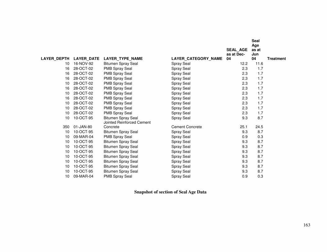
163
LAYER_DEPTH LAYER_DATE LAYER_TYPE_NAME LAYER_CATEGORY_NAME
SEAL_AGE as at Dec-04
Seal Age as at Jun 04 Treatment
10 16-NOV-92 Bitumen Spray Seal Spray Seal 12.2 11.6 16 28-OCT-02 PMB Spray Seal Spray Seal 2.3 1.7 16 28-OCT-02 PMB Spray Seal Spray Seal 2.3 1.7 16 28-OCT-02 PMB Spray Seal Spray Seal 2.3 1.7 10 28-OCT-02 PMB Spray Seal Spray Seal 2.3 1.7 16 28-OCT-02 PMB Spray Seal Spray Seal 2.3 1.7 10 28-OCT-02 PMB Spray Seal Spray Seal 2.3 1.7 16 28-OCT-02 PMB Spray Seal Spray Seal 2.3 1.7 10 28-OCT-02 PMB Spray Seal Spray Seal 2.3 1.7 10 28-OCT-02 PMB Spray Seal Spray Seal 2.3 1.7 10 28-OCT-02 PMB Spray Seal Spray Seal 2.3 1.7 10 10-OCT-95 Bitumen Spray Seal Spray Seal 9.3 8.7
350 01-JAN-80 Jointed Reinforced Cement Concrete Cement Concrete 25.1 24.5
10 10-OCT-95 Bitumen Spray Seal Spray Seal 9.3 8.7 10 09-MAR-04 PMB Spray Seal Spray Seal 0.9 0.3 10 10-OCT-95 Bitumen Spray Seal Spray Seal 9.3 8.7 10 10-OCT-95 Bitumen Spray Seal Spray Seal 9.3 8.7 10 10-OCT-95 Bitumen Spray Seal Spray Seal 9.3 8.7 10 10-OCT-95 Bitumen Spray Seal Spray Seal 9.3 8.7 10 10-OCT-95 Bitumen Spray Seal Spray Seal 9.3 8.7 10 10-OCT-95 Bitumen Spray Seal Spray Seal 9.3 8.7 10 10-OCT-95 Bitumen Spray Seal Spray Seal 9.3 8.7 10 09-MAR-04 PMB Spray Seal Spray Seal 0.9 0.3
Snapshot of section of Seal Age Data

164
ROAD_SECTION_ID CARRIAGEWAY_CODE START END LENGTH LAYER_NUMBER LAYER_TYPE LAYER_DEPTH LAYER_DATE LAYER_TYPE_NAME10F 1 149.4 149.45 0.05 1 K1 10 16-NOV-92 Bitumen Spray Seal 10F 1 149.45 149.455 0.005 1 K2 16 28-OCT-02 PMB Spray Seal 10F 1 149.455 149.485 0.03 1 K2 16 28-OCT-02 PMB Spray Seal 10F 1 149.485 149.75 0.265 1 K2 16 28-OCT-02 PMB Spray Seal 10F 1 149.75 150.05 0.3 1 K2 10 28-OCT-02 PMB Spray Seal 10F 1 150.05 150.35 0.3 1 K2 16 28-OCT-02 PMB Spray Seal 10F 1 150.35 150.65 0.3 1 K2 10 28-OCT-02 PMB Spray Seal 10F 1 150.65 150.95 0.3 1 K2 16 28-OCT-02 PMB Spray Seal 10F 1 150.95 151.15 0.2 1 K2 10 28-OCT-02 PMB Spray Seal 10F 1 151.15 151.45 0.3 1 K2 10 28-OCT-02 PMB Spray Seal 10F 1 151.45 151.535 0.085 1 K2 10 28-OCT-02 PMB Spray Seal 10F 1 151.535 158.654 7.119 1 K1 10 10-OCT-95 Bitumen Spray Seal
10F 1 158.654 158.726 0.072 1 E2 350 01-JAN-80 Jointed Reinforced Cement Concrete
10F 1 158.726 162.535 3.809 1 K1 10 10-OCT-95 Bitumen Spray Seal 10F 1 162.535 162.565 0.03 1 K2 10 09-MAR-04 PMB Spray Seal 10F 1 162.565 165.346 2.781 1 K1 10 10-OCT-95 Bitumen Spray Seal 10F 1 165.346 165.367 0.021 1 K1 10 10-OCT-95 Bitumen Spray Seal 10F 1 165.367 167.086 1.719 1 K1 10 10-OCT-95 Bitumen Spray Seal 10F 1 167.086 167.106 0.02 1 K1 10 10-OCT-95 Bitumen Spray Seal 10F 1 167.106 168.218 1.112 1 K1 10 10-OCT-95 Bitumen Spray Seal 10F 1 168.218 168.251 0.033 1 K1 10 10-OCT-95 Bitumen Spray Seal 10F 1 168.251 170.15 1.899 1 K1 10 10-OCT-95 Bitumen Spray Seal 10F 1 170.15 170.21 0.06 1 K2 10 09-MAR-04 PMB Spray Seal
Snapshot of section of Seal Type and Aggregate Size data

165
ROAD_SECTION_ID CARRIAGEWAY_CODE TDIST_START TDIST_END LENGTH SPEED_LIMIT 10F 1 149.4 177.81 28.41 110 10G 1 0.1 28.22 28.22 110 10G 1 28.22 56.74 28.52 100 10G 1 56.74 57.61 0.87 80 10G 1 57.61 97.92 40.31 100 10G 1 97.92 98.43 0.51 80 10G 1 98.43 99.05 0.62 60 10G 1 99.05 99.56 0.51 80 10G 1 99.56 118.15 18.59 100 10G 1 118.15 118.595 0.445 80 10G 1 118.595 119.935 1.34 70 10G 1 119.935 120.385 0.45 60 10G 1 120.385 120.55 0.165 50 10G 2 120.55 121.27 0.72 50 10G 1 121.27 121.415 0.145 50 10G 1 121.415 121.845 0.43 60 10G 1 121.845 122.145 0.3 80 10G 1 122.145 132.07 9.925 100 10G 1 132.07 132.97 0.9 80 10G 1 132.97 145.89 12.92 100 10G 1 145.89 150.275 4.385 90 10G 1 150.275 151.53 1.255 80
Snapshot of Section of the Speed Limit data

166
RSECT_ID LCODE_ID CCODE_ID TDIST_START TDIST_END LENGTH SPTD_OWP SPTD_BWP SPTD_IWP RATE_DATE 10F 1 1 149.4 149.5 0.1 3.27 4.15 05-MAY-04 10F 1 1 149.5 149.6 0.1 3.73 4.69 05-MAY-04 10F 1 1 149.6 149.7 0.1 3.42 4.46 05-MAY-04 10F 1 1 149.7 149.8 0.1 2.72 3.32 05-MAY-04 10F 1 1 149.8 149.9 0.1 2.54 2.69 05-MAY-04 10F 1 1 149.9 150 0.1 2.9 3.29 05-MAY-04 10F 1 1 150 150.1 0.1 3.05 4.26 05-MAY-04 10F 1 1 150.1 150.2 0.1 3.69 4.62 05-MAY-04 10F 1 1 150.2 150.3 0.1 3.54 4.06 05-MAY-04 10F 1 1 150.3 150.4 0.1 2.64 3.22 05-MAY-04 10F 1 1 150.4 150.5 0.1 2.24 2.71 05-MAY-04 10F 1 1 150.5 150.6 0.1 2.81 3.64 05-MAY-04 10F 1 1 150.6 150.7 0.1 3.91 4.77 05-MAY-04 10F 1 1 150.7 150.8 0.1 4.41 5.26 05-MAY-04 10F 1 1 150.8 150.9 0.1 3.89 4.67 05-MAY-04 10F 1 1 150.9 151 0.1 2.84 3.34 05-MAY-04 10F 1 1 151 151.1 0.1 2.34 2.85 05-MAY-04 10F 1 1 151.1 151.2 0.1 2.32 2.81 05-MAY-04 10F 1 1 151.2 151.3 0.1 2.29 2.74 05-MAY-04 10F 1 1 151.3 151.4 0.1 2.1 2.68 05-MAY-04 10F 1 1 151.4 151.45 0.05 1.85 2.51 05-MAY-04 10F 1 1 151.45 151.5 0.05 1.85 2.51 05-MAY-04 10F 1 1 151.5 151.6 0.1 1.73 2.49 05-MAY-04 10F 1 1 151.6 151.7 0.1 1.61 2.3 05-MAY-04
Snapshot of section of Surface Texture Depth Data

167
Appendix J Skid Resistance Field Inspection

167
Skid Resistance Investigation Form
Locality
Road Name Road Number
Tdist Start Tdist End
Geometry: Straight Curved
Intersection Open
Vertical Grade Superelevation
Aggregate Size
Inspected by: Date:
Factors Triggering Inspection
Skid Resistance Seal Age
Roughness Rutting
Accidents Drainage
Surface Texture Blackspot
Cracking Deformation
Public Complaint
Other (Specify)
Comments

168
Field Observations
Pavement Condition
Flushed Hungry Fair Good
Site Characteristics
Lighting is Inadequate / Adequate / Not Applicable
Visibility is Inadequate / Adequate
Delineation Inadequate / Adequate
Longitudinal Drainage is Inadequate / Needs Maintenance / Adequate
Cross Pavement Drainage is Inadequate / Adequate
Advanced Signage is Not Present / Present
Signage Condition is Poor / Fair / Good
Possible Mitigations
Speed Zone Signage
Reseal Surface Treatment
Line Marking Re-profile
Pavement Drainage
Other (Specify)
Comments
Recommendations
Action Required
Action Taken Date

169


