
Interpolated Delay Lines, Ideal Bandlimited Interpolation, and
Fractional Delay Filter Design
Julius Smith and Nelson Lee
RealSimple Project∗
Center for Computer Research in Music and Acoustics (CCRMA)Department of Music, Stanford University
Stanford, California 94305
June 5, 2008
∗Work supported by the Wallenberg Global Learning Network
1
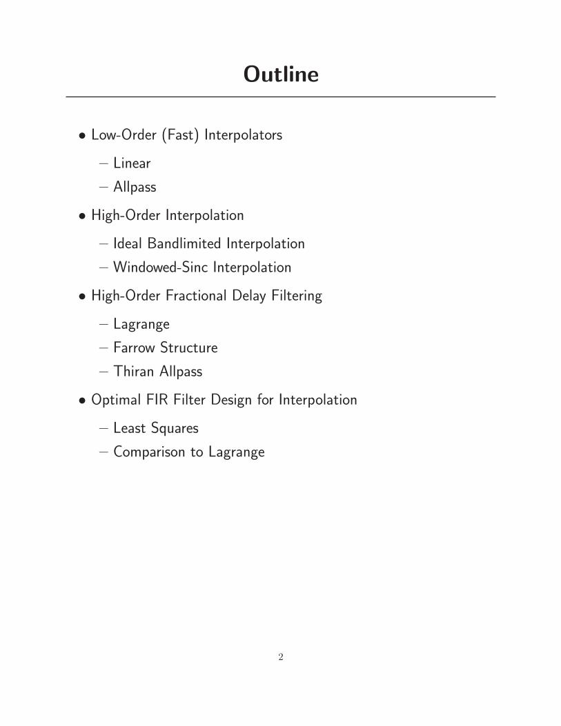
Outline
• Low-Order (Fast) Interpolators
– Linear
– Allpass
• High-Order Interpolation
– Ideal Bandlimited Interpolation
– Windowed-Sinc Interpolation
• High-Order Fractional Delay Filtering
– Lagrange
– Farrow Structure
– Thiran Allpass
• Optimal FIR Filter Design for Interpolation
– Least Squares
– Comparison to Lagrange
2
Simple Interpolators suitable for RealTime Fractional Delay Filtering
Linearly Interpolated Delay Line (1st-Order FIR)
M samples delay z−1
η
1 η−
y(n) ( )Mny η−−
Allpass Interpolated Delay Line (1st-Order)
M samples delay z−1y(n)
η
η−
( )Mny ∆−−
∆ ≈1− η
1 + η
3
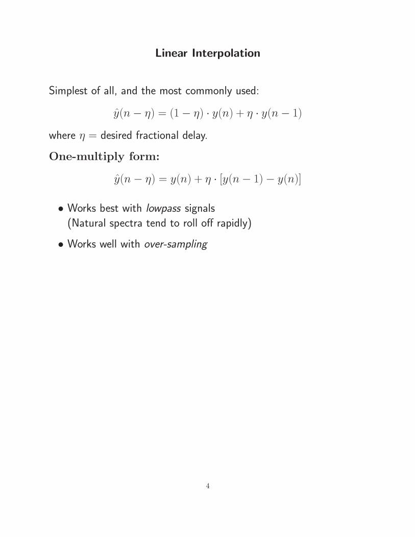
Linear Interpolation
Simplest of all, and the most commonly used:
y(n− η) = (1− η) · y(n) + η · y(n− 1)
where η = desired fractional delay.
One-multiply form:
y(n− η) = y(n) + η · [y(n− 1)− y(n)]
• Works best with lowpass signals
(Natural spectra tend to roll off rapidly)
• Works well with over-sampling
4
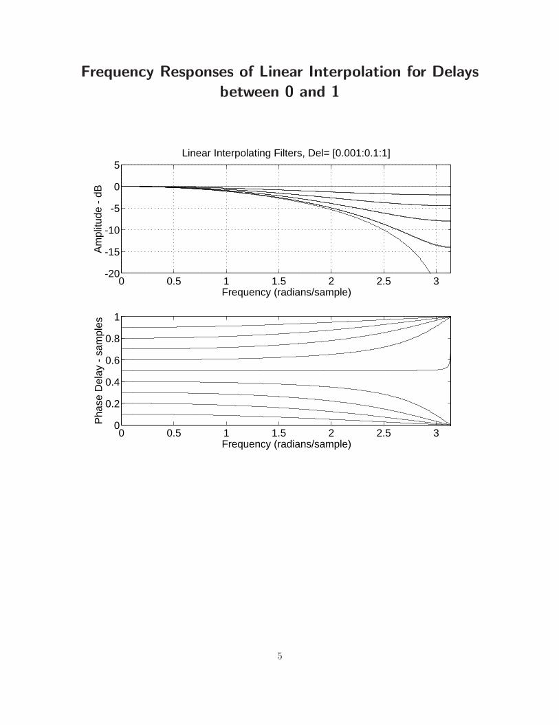
Frequency Responses of Linear Interpolation for Delays
between 0 and 1
0 0.5 1 1.5 2 2.5 3-20
-15
-10
-5
0
5Linear Interpolating Filters, Del= [0.001:0.1:1]
Frequency (radians/sample)
Am
plitu
de -
dB
0 0.5 1 1.5 2 2.5 30
0.2
0.4
0.6
0.8
1
Frequency (radians/sample)
Pha
se D
elay
- s
ampl
es
5

Linear Interpolation as a Convolution
Equivalent to filtering the continuous-time impulse train
N−1∑
n=0
y(nT )δ(t− nT )
with the continuous-time “triangular pulse” FIR filter
hl(t) =
1− |t/T | , |t| ≤ T
0, otherwise
followed by sampling at the desired phase
Replacing hl(t) by hs(t)∆= sinc
(
tT
)
converts linear interpolation to
ideal bandlimited interpolation (to be discussed later)
Upsample, Shift, Downsample View
z−LM M ( )ML
nx −( )nx
6
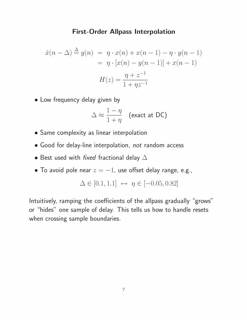
First-Order Allpass Interpolation
x(n−∆)∆= y(n) = η · x(n) + x(n− 1)− η · y(n− 1)
= η · [x(n)− y(n− 1)] + x(n− 1)
H(z) =η + z−1
1 + ηz−1
• Low frequency delay given by
∆ ≈1− η
1 + η(exact at DC)
• Same complexity as linear interpolation
• Good for delay-line interpolation, not random access
• Best used with fixed fractional delay ∆
• To avoid pole near z = −1, use offset delay range, e.g.,
∆ ∈ [0.1, 1.1] ↔ η ∈ [−0.05, 0.82]
Intuitively, ramping the coefficients of the allpass gradually “grows”
or “hides” one sample of delay. This tells us how to handle resets
when crossing sample boundaries.
7
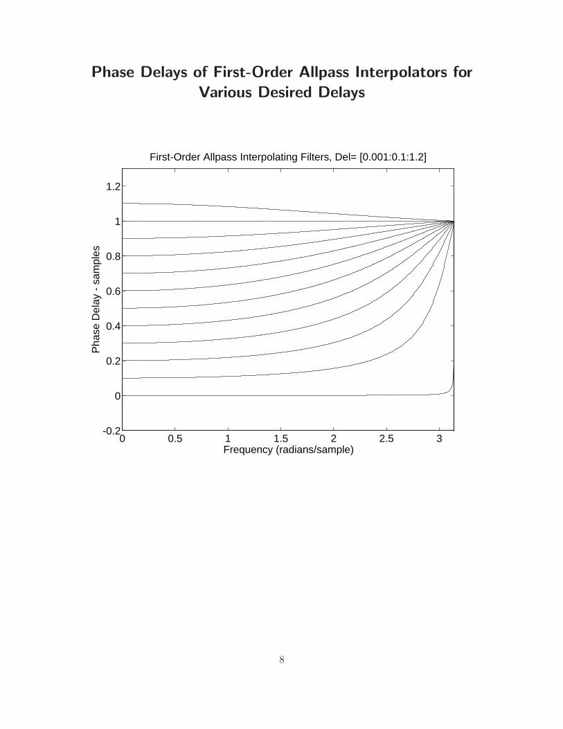
Phase Delays of First-Order Allpass Interpolators for
Various Desired Delays
0 0.5 1 1.5 2 2.5 3-0.2
0
0.2
0.4
0.6
0.8
1
1.2
First-Order Allpass Interpolating Filters, Del= [0.001:0.1:1.2]
Frequency (radians/sample)
Pha
se D
elay
- s
ampl
es
8
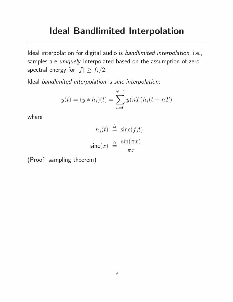
Ideal Bandlimited Interpolation
Ideal interpolation for digital audio is bandlimited interpolation, i.e.,
samples are uniquely interpolated based on the assumption of zero
spectral energy for |f | ≥ fs/2.
Ideal bandlimited interpolation is sinc interpolation:
y(t) = (y ∗ hs)(t) =
N−1∑
n=0
y(nT )hs(t− nT )
where
hs(t)∆= sinc(fst)
sinc(x)∆=
sin(πx)
πx
(Proof: sampling theorem)
9

Applications of Bandlimited Interpolation
Bandlimited Interpolation is used in (e.g.)
• Sampling-rate conversion
• Wavetable/sampling synthesis
• Virtual analog synthesis
• Oversampling D/A converters
• Fractional delay filtering
Fractional delay filtering is a special case of bandlimited
interpolation:
• Fractional delay filters only need sequential access ⇒ IIR filters
can be used
• General bandlimited interpolation requires random access ⇒ FIR
filters normally used
Fractional Delay Filters are used for (among other things)
• Time-varying delay lines (flanging, chorus, leslie)
• Resonator tuning in digital waveguide models
• Exact tonehole placement in woodwind models
• Beam steering of microphone / speaker arrays
10
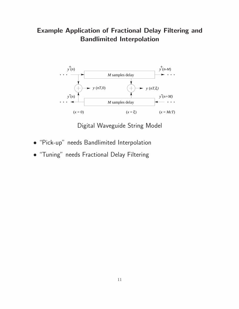
Example Application of Fractional Delay Filtering and
Bandlimited Interpolation
(x = 0)
. . .
. . .. . .
. . .y (n)-
y (n)+
y (nT,0) y (nT,ξ)
y (n-M)+
y (n+M)
(x = ξ) (x = McT)
M samples delay
M samples delay
-
Digital Waveguide String Model
• “Pick-up” needs Bandlimited Interpolation
• “Tuning” needs Fractional Delay Filtering
11
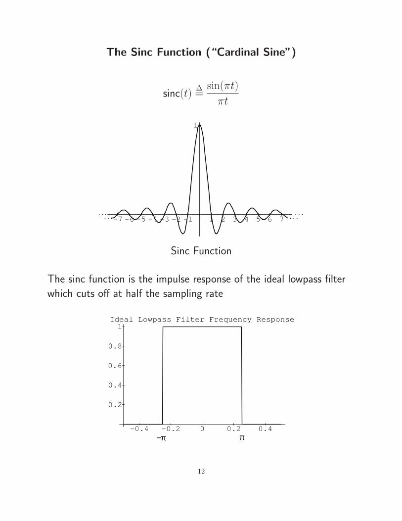
The Sinc Function (“Cardinal Sine”)
sinc(t)∆=
sin(πt)
πt
-7 -6 -5 -4 -3 -2 -1 1 2 3 4 5 6 7
1
. . .. . .
. . .. . .
Sinc Function
The sinc function is the impulse response of the ideal lowpass filter
which cuts off at half the sampling rate
Ideal Lowpass Filter Frequency Response
-0.4 -0.2 0 0.2 0.4
0.2
0.4
0.6
0.8
1
π−π
12
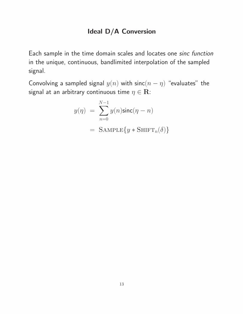
Ideal D/A Conversion
Each sample in the time domain scales and locates one sinc function
in the unique, continuous, bandlimited interpolation of the sampled
signal.
Convolving a sampled signal y(n) with sinc(n− η) “evaluates” the
signal at an arbitrary continuous time η ∈ R:
y(η) =
N−1∑
n=0
y(n)sinc(η − n)
= Sampley ∗ Shiftn(δ)
13

Ideal D/A Example
Reconstruction of a bandlimited rectangular pulse x(t) from its
samples x = [. . . , 0, 1, 1, 1, 1, 1, 0, . . .]:
Bandlimited Rectangular Pulse Reconstruction
Catch
• Sinc function is infinitely long and noncausal
• Must be available in continuous form
14

Optimal Least Squares Bandlimited Interpolation
Formulated as a Fractional Delay Filter
Note that interpolation is a special case of linear filtering. (Proof:
Convolution representation above.)
Consider a filter which delays its input by ∆ samples:
• Ideal impulse response = bandlimited delayed impulse = delayed
sinc
h∆(t) = sinc(t−∆)∆=
sin [π(t−∆)]
π(t−∆)
• Ideal frequency response = “brick wall” lowpass response,
cutting off at fs/2 and having linear phase e−jω∆T
H∆(ejω)∆= DTFT(h∆) =
e−jω∆, |ω| < πfs
0, |ω| ≥ πfs
→ H∆(ejωT ) = e−jω∆T , −π ≤ ωT < π
↔ sinc(n−∆), n = 0,±1,±2, . . .
The sinc function is an infinite-impulse-response (IIR) digital filter
with no recursive form ⇒ non-realizable
To obtain a finite impulse response (FIR) interpolating filter, let’s
formulate a least-squares filter-design problem:
15

Desired Interpolator Frequency Response
H∆
(
ejωT)
= e−jω∆T , ∆ = Desired delay in samples
FIR Filter Frequency Response
H∆
(
ejωT)
=
L−1∑
n=0
h∆(n)e−jωnT
Error to Minimize
E(
ejωT)
= H∆
(
ejωT)
− H∆
(
ejωT)
L2 Error Norm
J(h)∆= ‖E ‖22 =
T
2π
∫ π/T
−π/T
∣
∣E(
ejωT)∣
∣
2dω
=T
2π
∫ π/T
−π/T
∣
∣
∣H∆
(
ejωT)
− H∆
(
ejωT)
∣
∣
∣
2
dω
By Parseval’s Theorem
J(h) =
∞∑
n=0
∣
∣
∣h∆(n)− h∆(n)
∣
∣
∣
2
Optimal Least-Squares FIR Interpolator
h∆(n) =
sinc(n−∆), 0 ≤ n ≤ L− 1
0, otherwise
16
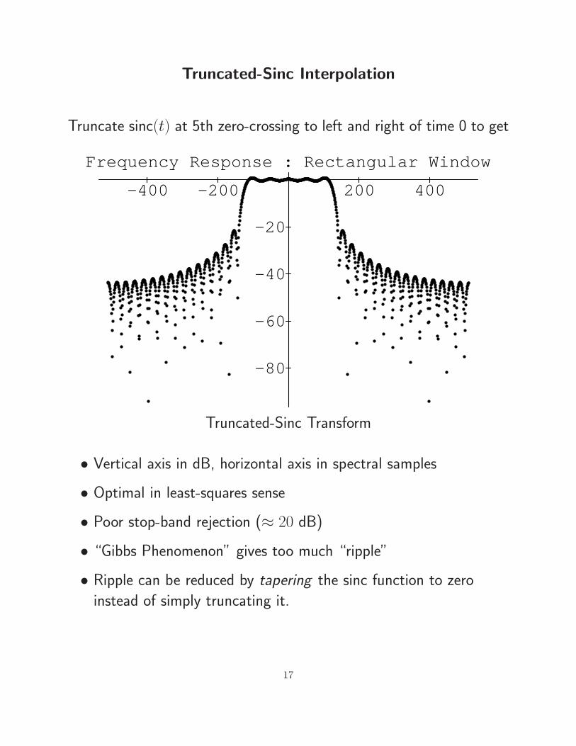
Truncated-Sinc Interpolation
Truncate sinc(t) at 5th zero-crossing to left and right of time 0 to get
Frequency Response : Rectangular Window
-400 -200 200 400
-80
-60
-40
-20
Truncated-Sinc Transform
• Vertical axis in dB, horizontal axis in spectral samples
• Optimal in least-squares sense
• Poor stop-band rejection (≈ 20 dB)
• “Gibbs Phenomenon” gives too much “ripple”
• Ripple can be reduced by tapering the sinc function to zero
instead of simply truncating it.
17
Windowed Sinc Interpolation
• Sinc function can be windowed more generally to yield
h∆(n) =
w(n−∆)sinc[α(n−∆)], 0 ≤ n ≤ L− 1
0, otherwise
• Example of window method for FIR lowpass filter design applied
to sinc functions (ideal lowpass filters) sampled at various phases
(corresponding to desired delay between samples)
• For best results, ∆ ≈ L/2
• w(n) is any real symmetric window (e.g., Hamming, Blackman,
Kaiser).
• Non-rectangular windows taper truncation which reduces Gibbs
phenomenon, as in FFT analysis
18

Spectrum of Kaiser-windowed Sinc
Frequency Response : Kaiser Window
-400 -200 200 400
-140
-120
-100
-80
-60
-40
-20
Kaiser-Windowed Sinc Transform
• Stopband now starts out close to −80 dB
• Kaiser window has a single parameter which trades off stop-band
attenuation versus transition-bandwidth from pass-band to
stop-band
19

Lowpass Filter Design
ω
Gain
ωc00
1
ωs2
TransitionBand
PassBand
StopBand
Frequency
Lowpass Filter Design Parameters
• In the transition band, frequency response “rolls off” from 1 at
ωc = ωs/(2α) to zero (or ≈ 0.5) at ωs/2.
• Interpolation can remain “perfect” in pass-band
Online references (FIR interpolator design)
• Music 421 Lecture 2 on Windows1
• Music 421 Lecture 3 on FIR Digital Filter Design2
• Optimal FIR Interpolator Design3
1http://ccrma.stanford.edu/˜jos/Windows/2http://ccrma.stanford.edu/˜jos/WinFlt/3http://ccrma.stanford.edu/ jos/resample/optfir.pdf
20
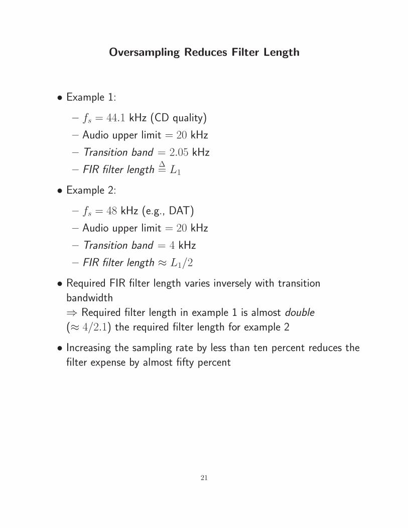
Oversampling Reduces Filter Length
• Example 1:
– fs = 44.1 kHz (CD quality)
– Audio upper limit = 20 kHz
– Transition band = 2.05 kHz
– FIR filter length∆= L1
• Example 2:
– fs = 48 kHz (e.g., DAT)
– Audio upper limit = 20 kHz
– Transition band = 4 kHz
– FIR filter length ≈ L1/2
• Required FIR filter length varies inversely with transition
bandwidth
⇒ Required filter length in example 1 is almost double
(≈ 4/2.1) the required filter length for example 2
• Increasing the sampling rate by less than ten percent reduces the
filter expense by almost fifty percent
21
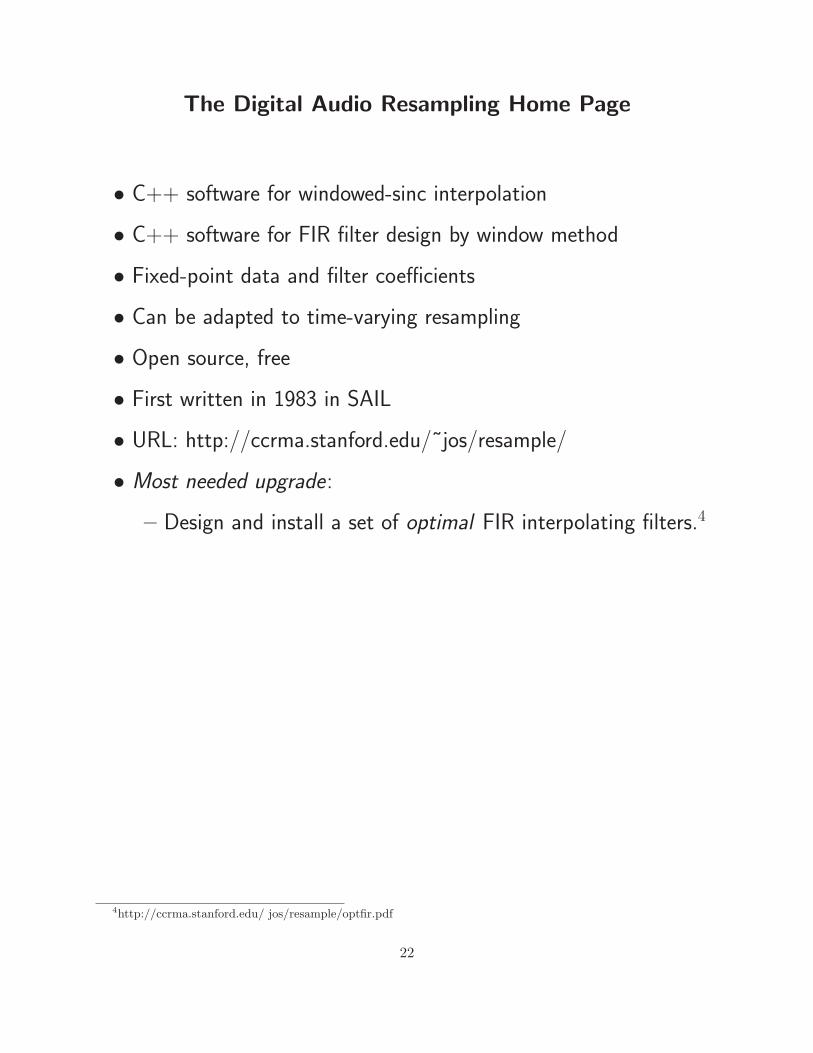
The Digital Audio Resampling Home Page
• C++ software for windowed-sinc interpolation
• C++ software for FIR filter design by window method
• Fixed-point data and filter coefficients
• Can be adapted to time-varying resampling
• Open source, free
• First written in 1983 in SAIL
• URL: http://ccrma.stanford.edu/˜jos/resample/
• Most needed upgrade:
– Design and install a set of optimal FIR interpolating filters.4
4http://ccrma.stanford.edu/ jos/resample/optfir.pdf
22
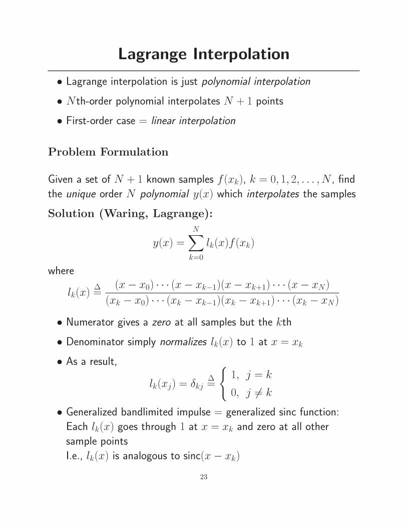
Lagrange Interpolation
• Lagrange interpolation is just polynomial interpolation
• N th-order polynomial interpolates N + 1 points
• First-order case = linear interpolation
Problem Formulation
Given a set of N + 1 known samples f(xk), k = 0, 1, 2, . . . , N , find
the unique order N polynomial y(x) which interpolates the samples
Solution (Waring, Lagrange):
y(x) =
N∑
k=0
lk(x)f(xk)
where
lk(x)∆=
(x− x0) · · · (x− xk−1)(x− xk+1) · · · (x− xN)
(xk − x0) · · · (xk − xk−1)(xk − xk+1) · · · (xk − xN)
• Numerator gives a zero at all samples but the kth
• Denominator simply normalizes lk(x) to 1 at x = xk
• As a result,
lk(xj) = δkj∆=
1, j = k
0, j 6= k
• Generalized bandlimited impulse = generalized sinc function:
Each lk(x) goes through 1 at x = xk and zero at all other
sample points
I.e., lk(x) is analogous to sinc(x− xk)
23
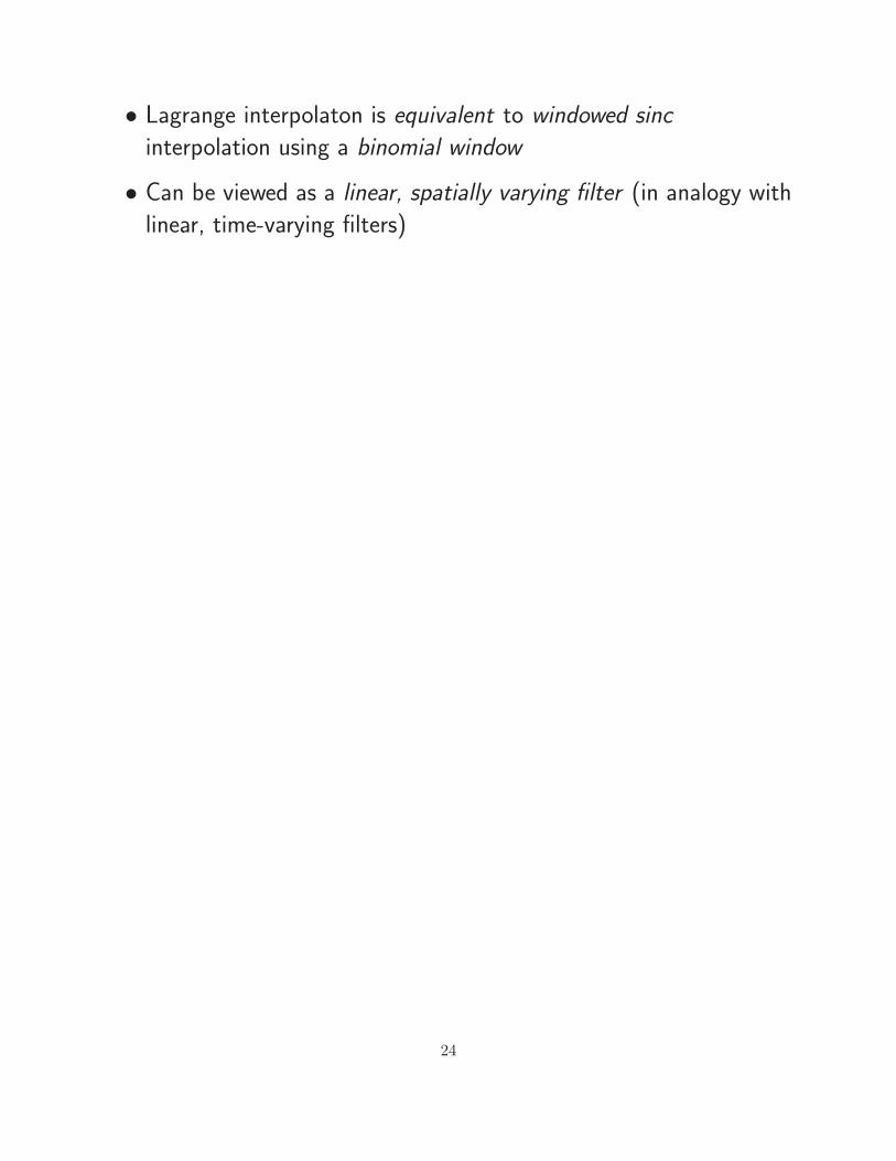
• Lagrange interpolaton is equivalent to windowed sinc
interpolation using a binomial window
• Can be viewed as a linear, spatially varying filter (in analogy with
linear, time-varying filters)
24
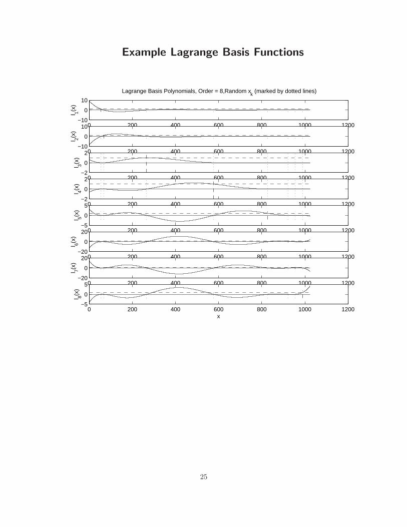
Example Lagrange Basis Functions
0 200 400 600 800 1000 1200−10
0
10
Lagrange Basis Polynomials, Order = 8,Random xk (marked by dotted lines)
l 1(x)
0 200 400 600 800 1000 1200−10
0
10
l 2(x)
0 200 400 600 800 1000 1200−2
0
2
l 3(x)
0 200 400 600 800 1000 1200−2
0
2
l 4(x)
0 200 400 600 800 1000 1200−5
0
5
l 5(x)
0 200 400 600 800 1000 1200−20
0
20
l 6(x)
0 200 400 600 800 1000 1200−20
0
20
l 7(x)
0 200 400 600 800 1000 1200−5
0
5
l 8(x)
x
25

Lagrange Interpolation Optimality
In the uniformly sampled case, Lagrange interpolation can be
viewed as ordinary FIR filtering:
– Lagrange interpolation filters maximally flat in the frequency
domain about dc:
dmE(ejω)
dωm
∣
∣
∣
∣
ω=0
= 0, m = 0, 1, 2, . . . , N,
where
E(ejω)∆= e−jω∆ −
N∑
n=0
h(n)e−jωn
and ∆ is the desired delay in samples.
– Same optimality criterion as Butterworth filters in classical
analog filter design
– Can also be viewed as “Pade approximation” to a constant
frequency response in the frequency domain
26
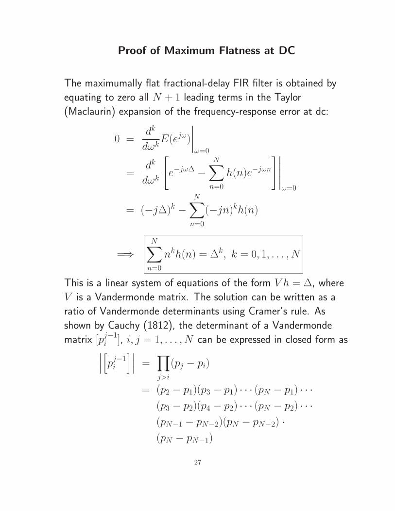
Proof of Maximum Flatness at DC
The maximumally flat fractional-delay FIR filter is obtained by
equating to zero all N + 1 leading terms in the Taylor
(Maclaurin) expansion of the frequency-response error at dc:
0 =dk
dωkE(ejω)
∣
∣
∣
∣
ω=0
=dk
dωk
[
e−jω∆ −
N∑
n=0
h(n)e−jωn
]∣
∣
∣
∣
∣
ω=0
= (−j∆)k −
N∑
n=0
(−jn)kh(n)
=⇒N
∑
n=0
nkh(n) = ∆k, k = 0, 1, . . . , N
This is a linear system of equations of the form V h = ∆, where
V is a Vandermonde matrix. The solution can be written as a
ratio of Vandermonde determinants using Cramer’s rule. As
shown by Cauchy (1812), the determinant of a Vandermonde
matrix [pj−1i ], i, j = 1, . . . , N can be expressed in closed form as
∣
∣
∣
[
pj−1i
]∣
∣
∣=
∏
j>i
(pj − pi)
= (p2 − p1)(p3 − p1) · · · (pN − p1) · · ·
(p3 − p2)(p4 − p2) · · · (pN − p2) · · ·
(pN−1 − pN−2)(pN − pN−2) ·
(pN − pN−1)
27
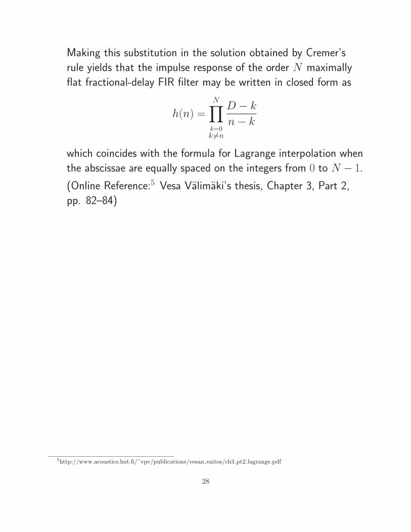
Making this substitution in the solution obtained by Cremer’s
rule yields that the impulse response of the order N maximally
flat fractional-delay FIR filter may be written in closed form as
h(n) =
N∏
k=0
k 6=n
D − k
n− k
which coincides with the formula for Lagrange interpolation when
the abscissae are equally spaced on the integers from 0 to N − 1.
(Online Reference:5 Vesa Valimaki’s thesis, Chapter 3, Part 2,
pp. 82–84)
5http://www.acoustics.hut.fi/˜vpv/publications/vesan vaitos/ch3 pt2 lagrange.pdf
28

Lagrange Interpolator Frequency Responses: Orders 1,
2, and 3
0 0.5 1 1.5 2 2.5 3 3.5−14
−12
−10
−8
−6
−4
−2
0Lagrange FIR Interpolating Filters, Del=1.4, Orders 1:3
Frequency (radians/sample)
Am
plitu
de −
dB
Order 1Order 2Order 3
0 0.5 1 1.5 2 2.5 3 3.5−2
−1.5
−1
−0.5
0
0.5
1
1.5
Frequency (radians/sample)
Gro
up D
elay
− s
ampl
es
Order 1Order 2Order 3
∆ = 1.4
29

Explicit Formula for Lagrange Interpolation Coefficients
h∆(n) =∏
k=0
k 6=n
∆− k
n− k, n = 0, 1, 2, . . . , N
Lagrange Interpolation Coefficients
Orders 1, 2, and 3
h∆Order h∆(0) h∆(1) h∆(2) h∆(3)
N = 1 1−∆ ∆
N = 2 (∆−1)(∆−2)2
−∆(∆− 2) ∆(∆−1)2
N = 3 − (∆−1)(∆−2)(∆−3)6
∆(∆−2)(∆−3)2
−∆(∆−1)(∆−3)2
∆(∆−1)(∆−2)6
– For N = 1, Lagrange interpolation reduces to linear
interpolation h = [1−∆, ∆], as before
– For order N , desired delay should be in a one-sample range
centered about ∆ = N/2
30
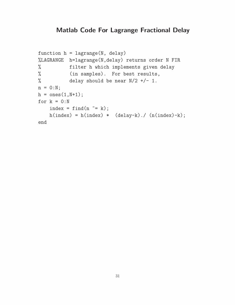
Matlab Code For Lagrange Fractional Delay
function h = lagrange(N, delay)
%LAGRANGE h=lagrange(N,delay) returns order N FIR
% filter h which implements given delay
% (in samples). For best results,
% delay should be near N/2 +/- 1.
n = 0:N;
h = ones(1,N+1);
for k = 0:N
index = find(n ~= k);
h(index) = h(index) * (delay-k)./ (n(index)-k);
end
31
Relation of Lagrange Interpolation toWindowed Sinc Interpolation
• For an infinite number of equally spaced samples, with spacing
xk+1 − xk = ∆, the Lagrange-interpolation basis polynomials
converge to shifts of the sinc function, i.e.,
lk(x) = sinc
(
x− k∆
∆
)
, k = . . . ,−2,−1, 0, 1, 2, . . .
Proof: As order →∞, the binomial window → Gaussian
window → constant (unity).
Alternate Proof: Every analytic function is determined by its
zeros and its value at one nonzero point. Since sin(πx) is zero
on all the integers except 0, and since sinc(0) = 1, it therefore
coincides with the Lagrangian basis polynomial for N =∞ and
k = 0.
32
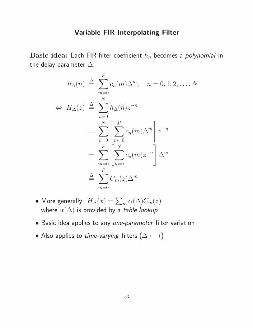
Variable FIR Interpolating Filter
Basic idea: Each FIR filter coefficient hn becomes a polynomial in
the delay parameter ∆:
h∆(n)∆=
P∑
m=0
cn(m)∆m, n = 0, 1, 2, . . . , N
⇔ H∆(z)∆=
N∑
n=0
h∆(n)z−n
=
N∑
n=0
[
P∑
m=0
cn(m)∆m
]
z−n
=
P∑
m=0
[
N∑
n=0
cn(m)z−n
]
∆m
∆=
P∑
m=0
Cm(z)∆m
• More generally: H∆(x) =∑
m α(∆)Cm(z)
where α(∆) is provided by a table lookup
• Basic idea applies to any one-parameter filter variation
• Also applies to time-varying filters (∆← t)
33
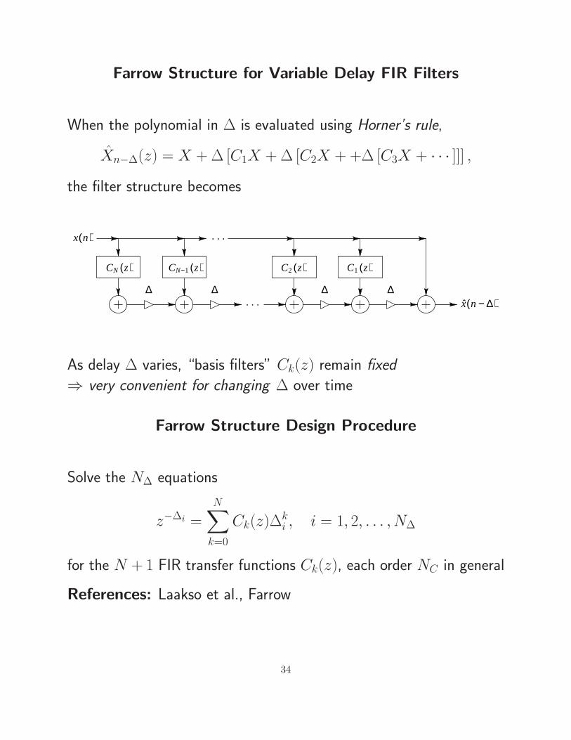
Farrow Structure for Variable Delay FIR Filters
When the polynomial in ∆ is evaluated using Horner’s rule,
Xn−∆(z) = X + ∆ [C1X + ∆ [C2X + +∆ [C3X + · · · ]]] ,
the filter structure becomes
( )nx
( )zCN ( )zC −N 1 ( )zC2 ( )zC1
( )nx ∆−∆ ∆ ∆ ∆
. . .
. . .
As delay ∆ varies, “basis filters” Ck(z) remain fixed
⇒ very convenient for changing ∆ over time
Farrow Structure Design Procedure
Solve the N∆ equations
z−∆i =
N∑
k=0
Ck(z)∆ki , i = 1, 2, . . . , N∆
for the N + 1 FIR transfer functions Ck(z), each order NC in general
References: Laakso et al., Farrow
34

Thiran Allpass Interpolators
Given a desired delay ∆ = N + δ samples, an order N allpass filter
H(z) =z−NA
(
z−1)
A(z)=
aN + aN−1z−1 + · · · + a1z
−(N−1) + z−N
1 + a1z−1 + · · · + aN−1z−(N−1) + aNz−N
can be designed having maximally flat group delay equal to ∆ at DC
using the formula
ak = (−1)k(
N
k
) N∏
n=0
∆−N + n
∆−N + k + n, k = 0, 1, 2, . . . , N
where(
N
k
)
=N !
k!(N − k)!
denotes the kth binomial coefficient
• a0 = 1 without further scaling
• For sufficiently large ∆, stability is guaranteed
rule of thumb: ∆ ≈ order
• Mean group delay is always N samples
(for any stable N th-order allpass filter):
1
2π
∫ 2π
0
D(ω)dω∆= −
1
2π
∫ 2π
0
Θ′(ω)dω = −1
2π[Θ(2π)− Θ(0)] = N
• Only known closed-form case for allpass interpolators of arbitrary
order
• Effective for delay-line interpolation needed for tuning since pitch
perception is most acute at low frequencies.
35
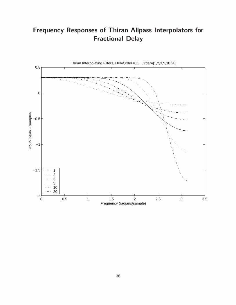
Frequency Responses of Thiran Allpass Interpolators for
Fractional Delay
0 0.5 1 1.5 2 2.5 3 3.5−2
−1.5
−1
−0.5
0
0.5Thiran Interpolating Filters, Del=Order+0.3, Order=[1,2,3,5,10,20]
Gro
up D
elay
− s
ampl
es
Frequency (radians/sample)
1 2 3 5 1020
36

Large Delay Changes
When implementing large delay-length changes (by many samples), a
useful implementation is to cross-fade from the initial delay line
configuration to the new configuration.
• Computation doubled during cross-fade
• Cross-fade should be long enough to sound smooth
• Not a true “morph” from one delay length to another, since we
do not pass through the intermediate delay lengths.
• A single delay line can be shared such that the cross-fade occurs
from one read-pointer (plus associated filtering) to another.
37
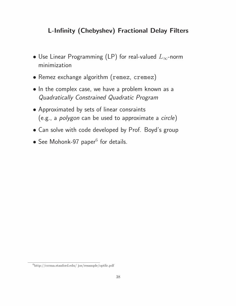
L-Infinity (Chebyshev) Fractional Delay Filters
• Use Linear Programming (LP) for real-valued L∞-norm
minimization
• Remez exchange algorithm (remez, cremez)
• In the complex case, we have a problem known as a
Quadratically Constrained Quadratic Program
• Approximated by sets of linear consraints
(e.g., a polygon can be used to approximate a circle)
• Can solve with code developed by Prof. Boyd’s group
• See Mohonk-97 paper6 for details.
6http://ccrma.stanford.edu/ jos/resample/optfir.pdf
38
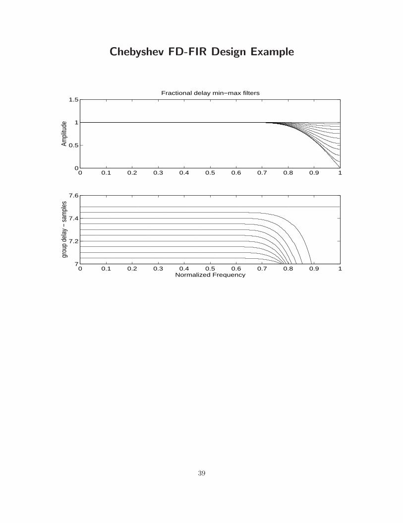
Chebyshev FD-FIR Design Example
0 0.1 0.2 0.3 0.4 0.5 0.6 0.7 0.8 0.9 17
7.2
7.4
7.6
Normalized Frequency
grou
p de
lay
− sa
mpl
es
0 0.1 0.2 0.3 0.4 0.5 0.6 0.7 0.8 0.9 10
0.5
1
1.5
Ampl
itude
Fractional delay min−max filters
39
0 5 10 15 20 25 300
0.002
0.004
0.006
0.008
0.01
0.012
0.014Modulus of the Error − (infinity norm)
40
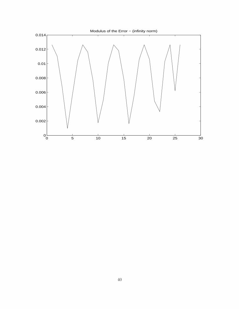
Comparison of Lagrange and OptimalChebyshev Fractional-Delay Filter
Frequency Responses
0 0.1 0.2 0.3 0.4 0.5 0.6 0.7 0.8 0.9 17
7.2
7.4
7.6
Normalized Frequency
grou
p de
lay
− s
ampl
es
0 0.1 0.2 0.3 0.4 0.5 0.6 0.7 0.8 0.9 10
0.5
1
Am
plitu
de
Comparison between min−maxs and Lagrange − L=16
41
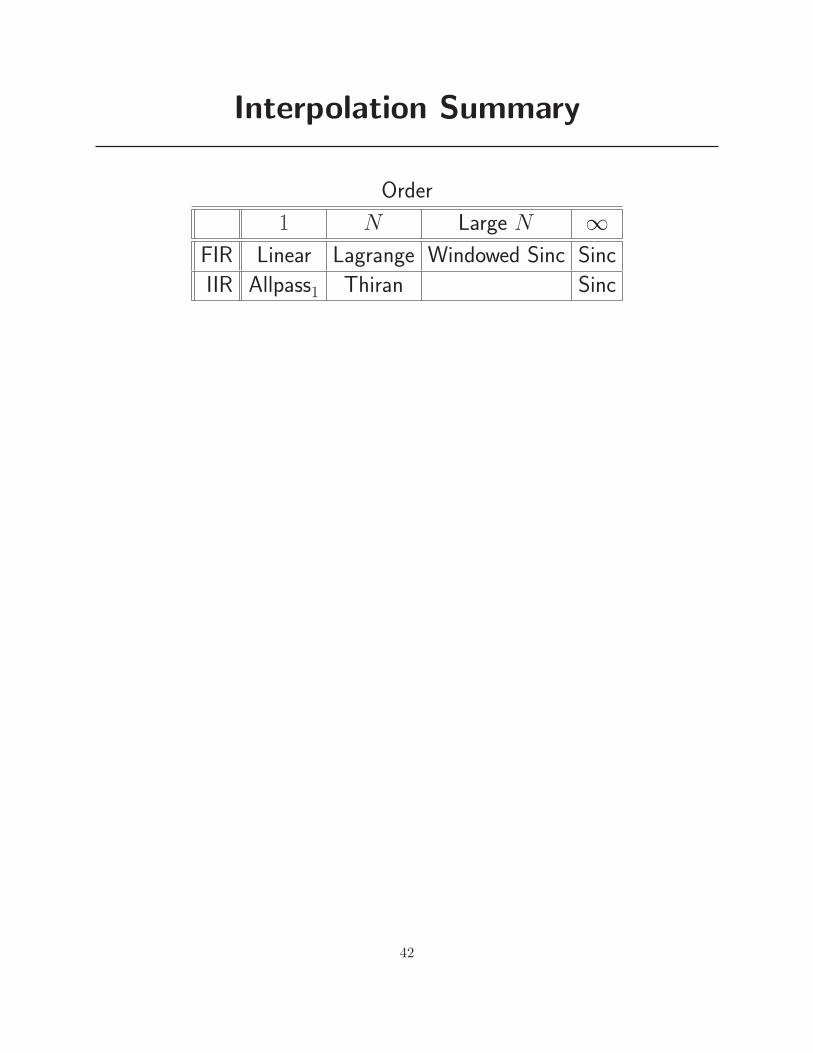
Interpolation Summary
Order
1 N Large N ∞
FIR Linear Lagrange Windowed Sinc Sinc
IIR Allpass1 Thiran Sinc
42


